cs 147: computer systems performance analysis - two …geoff/classes/hmc.cs147.201201/slides/... ·...

CS 147:Computer Systems Performance Analysis

Two-Factor Designs

1 / 34

CS 147:Computer Systems Performance Analysis

Two-Factor Designs

2015

-06-

15

CS147

Overview

Two-Factor DesignsNo ReplicationsAdding Replications

2 / 34

Overview

Two-Factor DesignsNo ReplicationsAdding Replications

2015

-06-

15

CS147

Overview

Two-Factor Designs No Replications

Two-Factor Design Without Replications

I Used when only two parameters, but multiple levels for eachI Test all combinations of levels of the two parametersI One replication (observation) per combinationI For factors A and B with a and b levels, ab experiments

required

3 / 34

Two-Factor Design Without Replications

I Used when only two parameters, but multiple levels for eachI Test all combinations of levels of the two parametersI One replication (observation) per combinationI For factors A and B with a and b levels, ab experiments

required

2015

-06-

15

CS147Two-Factor Designs

No ReplicationsTwo-Factor Design Without Replications


When to Use This Design?

I System has two important factorsI Factors are categoricalI More than two levels for at least one factorI Examples:

I Performance of different processors under different workloadsI Characteristics of different compilers for different benchmarksI Performance of different Web browsers on different sites

4 / 34

When to Use This Design?

I System has two important factorsI Factors are categoricalI More than two levels for at least one factorI Examples:

I Performance of different processors under different workloadsI Characteristics of different compilers for different benchmarksI Performance of different Web browsers on different sites

2015

-06-

15


No ReplicationsWhen to Use This Design?


When to Avoid This Design?

I Systems with more than two important factorsI Use general factorial design

I Non-categorical variablesI Use regression

I Only two levels per factorI Use 22 designs

5 / 34

When to Avoid This Design?

I Systems with more than two important factorsI Use general factorial design

I Non-categorical variablesI Use regression

I Only two levels per factorI Use 22 designs

2015

-06-

15


No ReplicationsWhen to Avoid This Design?


Model For This Design

I yij = µ+ αj + βi + eij

I yij is observationI µ is mean responseI αj is effect of factor A at level jI βi is effect of factor B at level iI eij is error termI Sums of αj ’s and βi ’s are both zero

6 / 34

Model For This Design

I yij = µ+ αj + βi + eij

I yij is observationI µ is mean responseI αj is effect of factor A at level jI βi is effect of factor B at level iI eij is error termI Sums of αj ’s and βi ’s are both zero

2015

-06-

15


No ReplicationsModel For This Design


Assumptions of the Model

I Factors are additiveI Errors are additiveI Typical assumptions about errors:

I Distributed independently of factor levelsI Normally distributed

I Remember to check these assumptions!

7 / 34

Assumptions of the Model

I Factors are additiveI Errors are additiveI Typical assumptions about errors:

I Distributed independently of factor levelsI Normally distributed

I Remember to check these assumptions!

2015

-06-

15


No ReplicationsAssumptions of the Model


Computing Effects

I Need to figure out µ, αj , and βiI Arrange observations in two-dimensional matrix

I b rows, a columnsI Compute effects such that error has zero mean

I Sum of error terms across all rows and columns is zero

8 / 34

Computing Effects

I Need to figure out µ, αj , and βiI Arrange observations in two-dimensional matrix

I b rows, a columnsI Compute effects such that error has zero mean

I Sum of error terms across all rows and columns is zero

2015

-06-

15


No ReplicationsComputing Effects


Two-Factor Full Factorial Example

I Want to expand functionality of a file system to allowautomatic compression

I Examine three choices:I Library substitution of file system callsI New VFSI Stackable layers

I Three different benchmarksI Metric: response time

9 / 34

Two-Factor Full Factorial Example

I Want to expand functionality of a file system to allowautomatic compression

I Examine three choices:I Library substitution of file system callsI New VFSI Stackable layers

I Three different benchmarksI Metric: response time

2015

-06-

15


No ReplicationsTwo-Factor Full Factorial Example


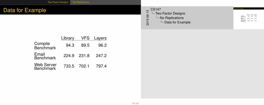
Data for Example

Library VFS LayersCompileBenchmark

94.3 89.5 96.2

EmailBenchmark 224.9 231.8 247.2

Web ServerBenchmark 733.5 702.1 797.4

10 / 34

Data for Example

Library VFS LayersCompileBenchmark

94.3 89.5 96.2

EmailBenchmark 224.9 231.8 247.2

Web ServerBenchmark 733.5 702.1 797.4

2015

-06-

15


No ReplicationsData for Example


Computing µ

I Averaging the j th column,

y ·j = µ+ αj +1b

∑i

βi +1b

∑i

eij

I By assumption, error terms add to zeroI Also, the βj ’s add to zero, so y ·j = µ+ αj

I Averaging rows produces y i· = µ+ βi

I Averaging everything produces y ·· = µ

11 / 34

Computing µ

I Averaging the j th column,

y ·j = µ+ αj +1b

∑i

βi +1b

∑i

eij

I By assumption, error terms add to zeroI Also, the βj ’s add to zero, so y ·j = µ+ αj

I Averaging rows produces y i· = µ+ βi

I Averaging everything produces y ·· = µ2015

-06-

15


No ReplicationsComputing µ


Model Parameters

Using same techniques as for one-factor designs, parameters are:

I y ·· = µ

I αj = y ·j − y ··I βi = y i· − y ··

12 / 34

Model Parameters

Using same techniques as for one-factor designs, parameters are:

I y ·· = µ

I αj = y ·j − y ··I βi = y i· − y ··

2015

-06-

15


No ReplicationsModel Parameters


Calculating Parameters for the Example

I µ = grand mean = 357.4I αj = (−6.5,−16.3,22.8)I βi = (−264.1,−122.8,386.9)I So, for example, the model predicts that the email benchmark

using a special-purpose VFS will take357.4− 16.3− 122.8 = 218.3 seconds

13 / 34

Calculating Parameters for the Example

I µ = grand mean = 357.4I αj = (−6.5,−16.3,22.8)I βi = (−264.1,−122.8,386.9)I So, for example, the model predicts that the email benchmark

using a special-purpose VFS will take357.4− 16.3− 122.8 = 218.3 seconds

2015

-06-

15


No ReplicationsCalculating Parameters for the Example


Estimating Experimental Errors

I Similar to estimation of errors in previous designsI Take difference between model’s predictions and

observationsI Calculate Sum of Squared ErrorsI Then allocate variation

14 / 34

Estimating Experimental Errors

I Similar to estimation of errors in previous designsI Take difference between model’s predictions and

observationsI Calculate Sum of Squared ErrorsI Then allocate variation

2015

-06-

15


No ReplicationsEstimating Experimental Errors


Allocating Variation

I Use same kind of procedure as on other modelsI SSY = SS0 + SSA + SSB + SSEI SST = SSY− SS0I Can then divide total variation between SSA, SSB, and SSE

15 / 34

Allocating Variation

I Use same kind of procedure as on other modelsI SSY = SS0 + SSA + SSB + SSEI SST = SSY− SS0I Can then divide total variation between SSA, SSB, and SSE

2015

-06-

15


No ReplicationsAllocating Variation


Calculating SS0, SSA, SSB

I SS0 = abµ2

I SSA = b∑

j α2j

I SSB = a∑

i β2i

I Recall that a and b are numbers of levels for the factors

16 / 34

Calculating SS0, SSA, SSB

I SS0 = abµ2

I SSA = b∑

j α2j

I SSB = a∑

i β2i

I Recall that a and b are numbers of levels for the factors

2015

-06-

15


No ReplicationsCalculating SS0, SSA, SSB


Allocation of Variation for Example

I SSE = 2512I SSY = 1,858,390I SS0 = 1,149,827I SSA = 2489I SSB = 703,561I SST = 708,562I Percent variation due to A: 0.35%I Percent variation due to B: 99.3%I Percent variation due to errors: 0.35%

17 / 34

Allocation of Variation for Example

I SSE = 2512I SSY = 1,858,390I SS0 = 1,149,827I SSA = 2489I SSB = 703,561I SST = 708,562I Percent variation due to A: 0.35%I Percent variation due to B: 99.3%I Percent variation due to errors: 0.35%20

15-0

6-15


No ReplicationsAllocation of Variation for Example


Analysis of Variation

I Again, similar to previous models, with slight modificationsI As before, use an ANOVA procedure

I Need extra row for second factorI Minor changes in degrees of freedom

I End steps are the sameI Compare F-computed to F-tableI Compare for each factor

18 / 34

Analysis of Variation

I Again, similar to previous models, with slight modificationsI As before, use an ANOVA procedure

I Need extra row for second factorI Minor changes in degrees of freedom

I End steps are the sameI Compare F-computed to F-tableI Compare for each factor

2015

-06-

15


No ReplicationsAnalysis of Variation


Analysis of Variation for Our Example

I MSE = SSE/[(a− 1)(b − 1)] = 2512/[(2)(2)] = 628I MSA = SSA/(a− 1) = 2489/2 = 1244I MSB = SSB/(b − 1) = 703,561/2 = 351,780I F-computed for A = MSA/MSE = 1.98I F-computed for B = MSB/MSE = 560I 95% F-table value for A & B is 6.94I So A is not significant, but B is

19 / 34

Analysis of Variation for Our Example

I MSE = SSE/[(a− 1)(b − 1)] = 2512/[(2)(2)] = 628I MSA = SSA/(a− 1) = 2489/2 = 1244I MSB = SSB/(b − 1) = 703,561/2 = 351,780I F-computed for A = MSA/MSE = 1.98I F-computed for B = MSB/MSE = 560I 95% F-table value for A & B is 6.94I So A is not significant, but B is

2015

-06-

15


No ReplicationsAnalysis of Variation for Our Example


Checking Our Results with Visual Tests

I As always, check if assumptions made in the analysis arecorrect

I Use residuals vs. predicted and quantile-quantile plots

20 / 34

Checking Our Results with Visual Tests

I As always, check if assumptions made in the analysis arecorrect

I Use residuals vs. predicted and quantile-quantile plots

2015

-06-

15


No ReplicationsChecking Our Results with Visual Tests


Residuals vs. Predicted Response for Example

0 200 400 600 800

-20

0

20

40

21 / 34

Residuals vs. Predicted Response for Example

0 200 400 600 800

-20

0

20

40

2015

-06-

15


No ReplicationsResiduals vs. Predicted Response forExample


What Does the Chart Reveal?

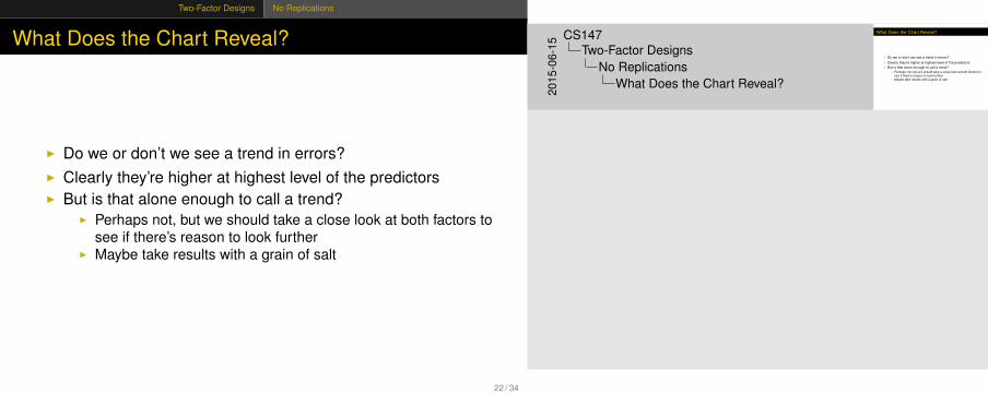
I Do we or don’t we see a trend in errors?I Clearly they’re higher at highest level of the predictorsI But is that alone enough to call a trend?

I Perhaps not, but we should take a close look at both factors tosee if there’s reason to look further

I Maybe take results with a grain of salt

22 / 34

What Does the Chart Reveal?

I Do we or don’t we see a trend in errors?I Clearly they’re higher at highest level of the predictorsI But is that alone enough to call a trend?

I Perhaps not, but we should take a close look at both factors tosee if there’s reason to look further

I Maybe take results with a grain of salt

2015

-06-

15


No ReplicationsWhat Does the Chart Reveal?


Quantile-Quantile Plot for Example

-2 -1 0 1 2

-40

-20

0

20

40

23 / 34

Quantile-Quantile Plot for Example

-2 -1 0 1 2

-40

-20

0

20

40

2015

-06-

15


No ReplicationsQuantile-Quantile Plot for Example


Confidence Intervals for Effects

I Need to determine standard deviation for data as a wholeI Then can derive standard deviations for effects

I Use different degrees of freedom for eachI Complete table in Jain, p. 351

24 / 34

Confidence Intervals for Effects

I Need to determine standard deviation for data as a wholeI Then can derive standard deviations for effects

I Use different degrees of freedom for eachI Complete table in Jain, p. 351

2015

-06-

15


No ReplicationsConfidence Intervals for Effects


Standard Deviations for Example

I se = 25I Standard deviation of µ:

sµ = se/√

ab = 25/√

3× 3 = 8.3

I Standard deviation of αj :

sαj = se√(a− 1)/ab = 25

√2/9 = 11.8

I Standard deviation of βi :

sβi = se√

(b − 1)/ab = 25√

2/9 = 11.8

25 / 34

Standard Deviations for Example

I se = 25I Standard deviation of µ:

sµ = se/√

ab = 25/√

3× 3 = 8.3

I Standard deviation of αj :

sαj = se√(a− 1)/ab = 25

√2/9 = 11.8

I Standard deviation of βi :

sβi = se√(b − 1)/ab = 25

√2/9 = 11.820

15-0

6-15


No ReplicationsStandard Deviations for Example


Calculating Confidence Intervals for Example

I Only file system alternatives shown hereI We’ll use 95% levelI 4 degrees of freedomI CI for library solution: (−39,26)I CI for VFS solution: (−49,16)I CI for layered solution: (−10,55)I So none of the solutions are significantly different from mean

at 95% confidence

26 / 34

Calculating Confidence Intervals for Example

I Only file system alternatives shown hereI We’ll use 95% levelI 4 degrees of freedomI CI for library solution: (−39,26)I CI for VFS solution: (−49,16)I CI for layered solution: (−10,55)I So none of the solutions are significantly different from mean

at 95% confidence2015

-06-

15


No ReplicationsCalculating Confidence Intervals for Example


Looking a Little Closer

I Do zero CI’s mean that none of the alternatives for addingfunctionality are different?

I Not necessarilyI Use contrasts to check (see Section 18.5 & p. 366)

27 / 34

Looking a Little Closer

I Do zero CI’s mean that none of the alternatives for addingfunctionality are different?

I Not necessarilyI Use contrasts to check (see Section 18.5 & p. 366)

2015

-06-

15


No ReplicationsLooking a Little Closer


Comparing Contrasts

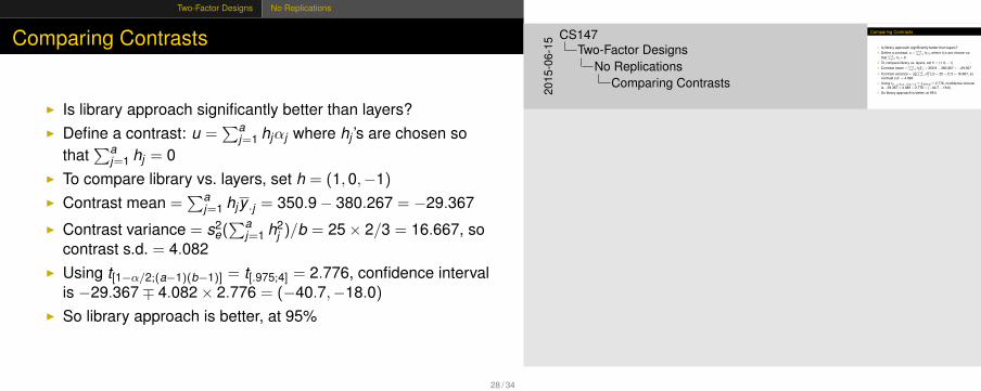
I Is library approach significantly better than layers?I Define a contrast: u =

∑aj=1 hjαj where hj ’s are chosen so

that∑a

j=1 hj = 0I To compare library vs. layers, set h = (1,0,−1)I Contrast mean =

∑aj=1 hjy ·j = 350.9− 380.267 = −29.367

I Contrast variance = s2e(∑a

j=1 h2j )/b = 25× 2/3 = 16.667, so

contrast s.d. = 4.082I Using t[1−α/2;(a−1)(b−1)] = t[.975;4] = 2.776, confidence interval

is −29.367∓ 4.082× 2.776 = (−40.7,−18.0)I So library approach is better, at 95%

28 / 34

Comparing Contrasts

I Is library approach significantly better than layers?I Define a contrast: u =

∑aj=1 hjαj where hj ’s are chosen so

that∑a

j=1 hj = 0I To compare library vs. layers, set h = (1,0,−1)I Contrast mean =

∑aj=1 hjy ·j = 350.9− 380.267 = −29.367

I Contrast variance = s2e(∑a

j=1 h2j )/b = 25× 2/3 = 16.667, so

contrast s.d. = 4.082I Using t[1−α/2;(a−1)(b−1)] = t[.975;4] = 2.776, confidence interval

is −29.367∓ 4.082× 2.776 = (−40.7,−18.0)I So library approach is better, at 95%20

15-0

6-15


No ReplicationsComparing Contrasts


Missing Observations

I Sometimes experiments go awryI You don’t want to discard an entire study away just because

one observation got lostI Solution:

I Calculate row/column means and standard deviations basedon actual observation count

I Degrees of freedom in SS* also must be adjustedI See book for example

I Alternatives exist but are controversialI If lots of missing values in a column or row, throw it out

entirelyI Best is to have only 1–2 missing values

29 / 34

Missing Observations

I Sometimes experiments go awryI You don’t want to discard an entire study away just because

one observation got lostI Solution:

I Calculate row/column means and standard deviations basedon actual observation count

I Degrees of freedom in SS* also must be adjustedI See book for example

I Alternatives exist but are controversialI If lots of missing values in a column or row, throw it out

entirelyI Best is to have only 1–2 missing values20

15-0

6-15


No ReplicationsMissing Observations

Two-Factor Designs Adding Replications

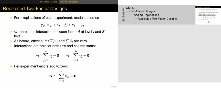
Replicated Two-Factor Designs

I For r replications of each experiment, model becomes

yijk = µ+ αj + βi + γij + eijk

I γij represents interaction between factor A at level j and B atlevel i

I As before, effect sums∑αj and

∑βi are zero

I Interactions are zero for both row and column sums:

∀ia∑

j=1

γij = 0 ∀jb∑

i=1

γij = 0

I Per-experiment errors add to zero:

∀i , jr∑

k=1

eijk = 0

30 / 34

Replicated Two-Factor Designs

I For r replications of each experiment, model becomes

yijk = µ+ αj + βi + γij + eijk

I γij represents interaction between factor A at level j and B atlevel i

I As before, effect sums∑αj and

∑βi are zero

I Interactions are zero for both row and column sums:

∀ia∑

j=1

γij = 0 ∀jb∑

i=1

γij = 0

I Per-experiment errors add to zero:

∀i , jr∑

k=1

eijk = 0

2015

-06-

15


Adding ReplicationsReplicated Two-Factor Designs


Calculating Effects

Same as usual:I Calculate grand mean y ···, row and column means y i·· and y ·j·

and per-experiment means y ij·I µ = y ···I αj = y ·j· − µI βi = y i·· − µI γij = y ij· − αj − βi − µI eijk = yijk − y ij·

31 / 34

Calculating Effects

Same as usual:I Calculate grand mean y ···, row and column means y i·· and y ·j·

and per-experiment means y ij·I µ = y ···I αj = y ·j· − µI βi = y i·· − µI γij = y ij· − αj − βi − µI eijk = yijk − y ij·20

15-0

6-15


Adding ReplicationsCalculating Effects


Analysis of Variance

I Again, extension of earlier modelsI See Table 22.5, p. 375, for formulasI As usual, must do visual tests

32 / 34

Analysis of Variance

I Again, extension of earlier modelsI See Table 22.5, p. 375, for formulasI As usual, must do visual tests

2015

-06-

15


Adding ReplicationsAnalysis of Variance


Why Can We Find Interactions?

I Without replications, two-factor model didn’t give interactionsI Why not?

I Insufficient dataI Variation from predictions was attributed to errors, not

interactionI Interaction is confounded with errors

I Now, we have more infoI For given A, B setting, errors are assumed to cause variation

in r replicated experimentsI Any remaining variation must therefore be interaction

33 / 34


I Without replications, two-factor model didn’t give interactionsI Why not?

I Insufficient dataI Variation from predictions was attributed to errors, not




2015

-06-

15


Adding ReplicationsWhy Can We Find Interactions?

This slide has animations.

In unreplicated experiment, we couldhave assumed no experimental errorsand attributed variation to interactioninstead (but that wouldn’t be wise).



I Without replications, two-factor model didn’t give interactionsI Why not?I Insufficient dataI Variation from predictions was attributed to errors, not




33 / 34


I Without replications, two-factor model didn’t give interactionsI Why not?I Insufficient dataI Variation from predictions was attributed to errors, not



in r replicated experimentsI Any remaining variation must therefore be interaction20

15-0

6-15


Adding ReplicationsWhy Can We Find Interactions?

This slide has animations.

In unreplicated experiment, we couldhave assumed no experimental errorsand attributed variation to interactioninstead (but that wouldn’t be wise).


General Full Factorial Designs

I Straightforward extension of two-factor designsI Average along axes to get effectsI Must consider all interactions (various axis combinations)I Regression possible for quantitative effects

I But should have more than three data pointsI If no replications, errors confounded with highest-level

interaction

34 / 34

General Full Factorial Designs

I Straightforward extension of two-factor designsI Average along axes to get effectsI Must consider all interactions (various axis combinations)I Regression possible for quantitative effects

I But should have more than three data pointsI If no replications, errors confounded with highest-level

interaction

2015

-06-

15


Adding ReplicationsGeneral Full Factorial Designs

cs 147: computer systems performance analysis - two …geoff/classes/hmc.cs147.201201/slides/... ·...

Documents