crystal structure and dynamics - university of oxford · description of the crystal structure and...
TRANSCRIPT

Crystal Structure and DynamicsPaolo G. Radaelli, Michaelmas Term 2013
Part 1: Symmetry in the solid stateLectures 1-4
Web Site:http://www2.physics.ox.ac.uk/students/course-materials/c3-condensed-matter-major-option
Bibliography
◦ C. Hammond The Basics of Crystallography and Diffraction, Oxford University Press (fromBlackwells). A well-established textbook for crystallography and diffraction.
◦ Paolo G. Radaelli, Symmetry in Crystallography: Understanding the International Tables ,Oxford University Press (2011). Contains much of the same materials covering lectures1-3, but in an extended form.
◦ T. Hahn, ed., International tables for crystallography, vol. A (Kluver Academic Publisher,Dodrecht: Holland/Boston: USA/ London: UK, 2002), 5th ed. The International Tables forCrystallography are an indispensable text for any condensed-matter physicist. It currentlyconsists of 8 volumes. A selection of pages is provided on the web site. Additional samplepages can be found on http://www.iucr.org/books/international-tables.
◦ C. Giacovazzo, H.L. Monaco, D. Viterbo, F. Scordari, G. Gilli, G. Zanotti and M. Catti, Fun-damentals of crystallography (International Union of Crystallography, Oxford UniversityPress Inc., New York)
◦ ”Visions of Symmetry: Notebooks, Periodic Drawings, and Related Work of M. C. Escher”,W.H.Freeman and Company, 1990. A collection of symmetry drawings by M.C. Escher,also to be found here:http://www.mcescher.com/Gallery/gallery-symmetry.htm
◦ Neil W. Ashcroft and N. David Mermin, Solid State Physics, HRW International Editions,CBS Publishing Asia Ltd (1976) is now a rather old book, but, sadly, it is probably still thebest solid-state physics book around. It is a graduate-level book, but it is accessible tothe interested undergraduate.
1

Contents
1 Lecture 1 — Symmetry of simple patterns 31.1 Introduction to group theory . . . . . . . . . . . . . . . . . . . . . . . . . . . . . . 31.2 Symmetry of periodic patterns in 2 dimensions: 2D point groups and wallpaper
groups . . . . . . . . . . . . . . . . . . . . . . . . . . . . . . . . . . . . . . . . . . 51.3 Combinations of rotations and translations — normal form of symmetry operators 9
2 Lecture 2 — Coordinates and calculations 122.1 Crystallographic coordinates . . . . . . . . . . . . . . . . . . . . . . . . . . . . . 122.2 Distances and angles . . . . . . . . . . . . . . . . . . . . . . . . . . . . . . . . . 132.3 Dual basis and coordinates . . . . . . . . . . . . . . . . . . . . . . . . . . . . . . 142.4 Dual basis in 3D . . . . . . . . . . . . . . . . . . . . . . . . . . . . . . . . . . . . 152.5 Dot products in reciprocal space . . . . . . . . . . . . . . . . . . . . . . . . . . . 152.6 A very useful example: the hexagonal system in 2D . . . . . . . . . . . . . . . . 162.7 Symmetry in 3 dimensions . . . . . . . . . . . . . . . . . . . . . . . . . . . . . . . 16
3 Lecture 3 — Fourier transform of periodic functions 223.1 Centring extinctions . . . . . . . . . . . . . . . . . . . . . . . . . . . . . . . . . . 223.2 Fourier transform of lattice functions . . . . . . . . . . . . . . . . . . . . . . . . . 233.3 The symmetry of |F (q)|2 and the Laue classes . . . . . . . . . . . . . . . . . . . 24
4 Lecture 4 — Brillouin zones and the symmetry of the band structure 264.1 Symmetry of the electronic band structure . . . . . . . . . . . . . . . . . . . . . . 274.2 Symmetry properties of the group velocity . . . . . . . . . . . . . . . . . . . . . . 29
4.2.1 The oblique lattice in 2D: a low symmetry case . . . . . . . . . . . . . . . 304.2.2 The square lattice: a high symmetry case . . . . . . . . . . . . . . . . . . 31
4.3 Symmetry in the nearly-free electron model: degenerate wavefunctions . . . . . 31
2

1 Lecture 1 — Symmetry of simple patterns
1.1 Introduction to group theory
• Previous courses have already illustrated the important of translational sym-metry (lattice periodicity), especially in the context of the Bloch theorem.Here, we will extend this by illustrating the important of rotational sym-metry :
• Knowing the full crystal symmetry (translation + rotation) allows a simplifieddescription of the crystal structure and calculations of its properties (interms of fewer unique atoms).
� Diffraction experiments can help to identify the crystal symmetry (al-beit not uniquely).
� Symmetry applies to continuous functions (e.g., electron density in acrystal) as well as to collections of discrete objects (atoms).
� The crystal symmetry generates a corresponding symmetry of thedispersion relations (phonons, electrons) in reciprocal space. Inthe spirit of describing real experiments, this means that smallerregions of the reciprocal space need to be measured (a quadrant,an octant etc.) to reconstruct the whole dispersion. Symmetry alsorestricts, for example, certain components of the group velocity.
• In describing the symmetry of isolated objects or periodic systems, onedefines operations (or operators) that describe transformations of thepattern. We create the new pattern from the old pattern by associat-ing a point p2 to each point p1 and transferring the “attributes” of p1to p2. This transformation preserves distances and angles, and is inessence a combination of translations, reflections and rotations. If thetransformation is a symmetry operator, the old and new patterns areindistinguishable.
• Symmetry operators can be applied one after the other, generating new op-erators. Taken all together they form a finite (for pure rotations/reflections)or infinite (if one includes translations) consistent set.
• The set of operators describing the symmetry of an object or pattern con-forms to the mathematical structure of a group. We will only deal withsets of operators, not with the more abstract mathematical concept ofgroup. A group is a set of elements with a defined binary operationknown as composition, which obeys certain rules.
3

� A binary operation (usually called composition or multiplication)must be defined. We indicated this with the symbol “◦”. Whengroup elements are operators, the operator to the right is appliedfirst.
� Composition must be associative: for every three elements f , g andh of the set
f ◦ (g ◦ h) = (f ◦ g) ◦ h (1)
� The “neutral element” (i.e., the identity, usually indicated with E) mustexist, so that for every element g:
g ◦ E = E ◦ g = g (2)
� Each element g has an inverse element g−1 so that
g ◦ g−1 = g−1 ◦ g = E (3)
� A subgroup is a subset of a group that is also a group.
� A set of generators is a subset of the group (not usually a subgroup)that can generate the whole group by composition. Infinite groups(e.g., the set of all lattice translations) can have a finite set of gen-erators (the primitive translations).
• Composition of two symmetry operators is the application of these one afteranother. we can see that the rules above hold.
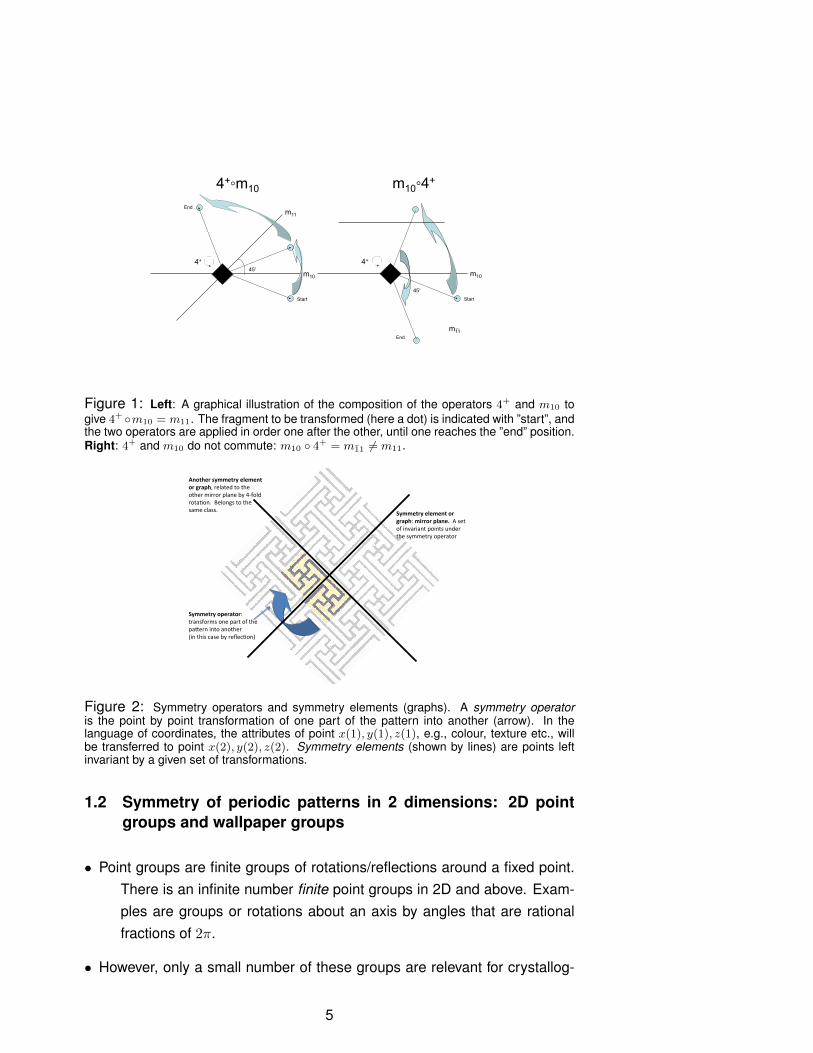
• Composition is not commutative (fig. 1).
• Graphs or symmetry elements are sets of invariant points of a pattern un-der one or more symmetry operators.
• Sets of symmetry-related graphs form a class. In group theory, they corre-spond to classes of symmetry operators, defined as follows: two sym-metry operators belong to the same class when they are conjugated. h′
is conjugated with h if there is a g ∈ G so that:
h′ = g ◦ h ◦ g−1 (4)
• Conjugation of graphs defines set of equivalent points with special proper-ties. Wychoff letters are used to label these points.
4
m10 45º
m11
4+
������
����
m10 4+
������
����
45º
m11
m10◦4+ 4+◦m10
Figure 1: Left: A graphical illustration of the composition of the operators 4+ and m10 togive 4+ ◦m10 = m11. The fragment to be transformed (here a dot) is indicated with ”start”, andthe two operators are applied in order one after the other, until one reaches the ”end” position.Right: 4+ and m10 do not commute: m10 ◦ 4+ = m1̄1 6= m11.
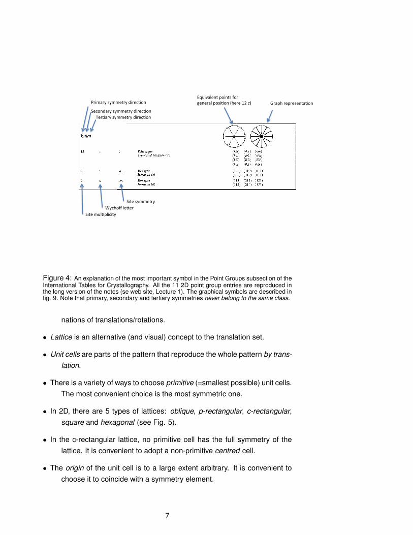
Symmetry operator: transforms one part of the pa.ern into another (in this case by reflec5on)
Symmetry element or graph: mirror plane. A set of invariant points under the symmetry operator
Another symmetry element or graph, related to the other mirror plane by 4-‐fold rota5on. Belongs to the same class.
Figure 2: Symmetry operators and symmetry elements (graphs). A symmetry operatoris the point by point transformation of one part of the pattern into another (arrow). In thelanguage of coordinates, the attributes of point x(1), y(1), z(1), e.g., colour, texture etc., willbe transferred to point x(2), y(2), z(2). Symmetry elements (shown by lines) are points leftinvariant by a given set of transformations.
1.2 Symmetry of periodic patterns in 2 dimensions: 2D pointgroups and wallpaper groups
• Point groups are finite groups of rotations/reflections around a fixed point.There is an infinite number finite point groups in 2D and above. Exam-ples are groups or rotations about an axis by angles that are rationalfractions of 2π.
• However, only a small number of these groups are relevant for crystallog-
5

Figure 3: Left. A showflake by by Vermont scientist-artist Wilson Bentley, c. 1902. RightThe symmetry group of the snowflake, 6mm in the ITC notation. The group has 6 classes, 5marked on the drawing plus the identity operator E. Note that there are two classes of mirrorplanes, marked “1” and “2” on the drawing. One can see on the snowflake picture that theirgraphs contain different patterns.
Table 1: The 17 wallpaper groups. The symbols are obtained by combiningthe 5 Bravais lattices with the 10 2D point groups, and replacing g with msystematically. Strikeout symbols are duplicate of other symbols.crystal system crystal class wallpaper groups
oblique1 p12 p2
rectangularm pm, cm,pg, cg
2mm p2mm, p2mg (=p2gm), p2gg, c2mm, c2mg, c2gg
square4 p4
4mm p4mm, p4gm, p4mg
hexagonal3 p3
3m1-31m p3m1, p3mg, p31m, p31g6 p6
6mm p6mm, p6mg, p6gm, p6gg
raphy, since all others are incompatible with a lattice. There are 10crystallographic point groups in 2D and 32 in 3D (see web site for acomplete list of crystallographic point groups and their properties fromthe ITC)1.
• Periodic patterns are invariant by a set of translations, which also form agroup. They may also be invariant by rotations/reflections and combi-
1A very interesting set of “sub-periodic” groups is represented by the so-called friezegroups, which describe the symmetry of a repeated pattern in 1 dimension. There are only7 frieze groups, which are very simple to understand given the small number of operatorsinvolved. For a description of the frieze groups, with some nice pictorial example, see theSupplementary Material.
6
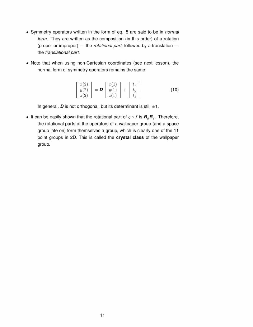
Graph representa+on
Secondary symmetry direc+on Ter+ary symmetry direc+on
Site mul+plicity Wychoff le8er
Site symmetry
Equivalent points for general posi+on (here 12 c) Primary symmetry direc+on
Figure 4: An explanation of the most important symbol in the Point Groups subsection of theInternational Tables for Crystallography. All the 11 2D point group entries are reproduced inthe long version of the notes (se web site, Lecture 1). The graphical symbols are described infig. 9. Note that primary, secondary and tertiary symmetries never belong to the same class.
nations of translations/rotations.
• Lattice is an alternative (and visual) concept to the translation set.
• Unit cells are parts of the pattern that reproduce the whole pattern by trans-lation.
• There is a variety of ways to choose primitive (=smallest possible) unit cells.The most convenient choice is the most symmetric one.
• In 2D, there are 5 types of lattices: oblique, p-rectangular, c-rectangular,square and hexagonal (see Fig. 5).
• In the c-rectangular lattice, no primitive cell has the full symmetry of thelattice. It is convenient to adopt a non-primitive centred cell.
• The origin of the unit cell is to a large extent arbitrary. It is convenient tochoose it to coincide with a symmetry element.
7

�p�� �c�
Oblique
Rectangular
Square Hexagonal
Figure 5: The 5 Bravails lattices in 2 dimensions.
• Although there are an infinite number of symmetry operators (and symme-try elements), it is sufficient to consider elements in a single unit cell.
• Glides. This is a composite symmetry, which combines a translation witha parallel reflection, neither of which on its own is a symmetry operator.In 2D groups, the glide is indicated with the symbol g. Twice a glidetranslation is always a symmetry translation: in fact, if one applies theglide operator twice as in g ◦ g, one obtains a pure translation (since thetwo mirrors cancel out), which therefore must be a symmetry translation.
• Walpaper groups. The 17 Plane (or Wallpaper) groups describe the sym-metry of all periodic 2D patterns (see tab. 1). The decision three in fig.6 can be used to identify wallpaper groups. 2
2For a more complete description of wallpaper groups and of the symmetry of the underly-ing 2D lattices, see the Supplementary Material.
8

64
Has
mir
rors
?
32
Has
mir
rors
?H
as m
irro
rs?
Has
mir
rors
?
p6p6
mm
Axe
s o
n
mir
rors
?
p4
p4m
mp4
gm
All
axes
on
mir
rors
?
p3
p3m
1
1
p31m
Has
ort
ho
go
nal
mir
rors
?
Has
glid
es?
p2p2
gg p2m
g
Has
ro
tati
on
so
ff m
irro
s?
c2m
mp2
mm
Has
mir
rors
?
Has
glid
es?
pm
cm
Has
glid
es?
pg
p1
Axi
s o
f h
igh
est
ord
er
Figure 6: Decision-making tree to identify wallpaper patterns. The first step (bottom) is toidentify the axis of highest order. Continuous and dotted lines are ”Yes” and ”No” branches,respectively. Diamonds are branching points.
1.3 Combinations of rotations and translations — normal formof symmetry operators
• Our aim here is to show that all symmetry operators can be written as thecomposition of a rotation (first) followed by a translation second. Wewill do this by employing Cartesian coordinates (we will generalise to
9

the 3D case).
• We have so far seen two combinations or rotations and translations:
� Glides are an example of roto-translations. In Cartesian coordinates,roto-translations can be written as:
x(2)y(2)z(2)
= R
x(1)y(1)z(1)
+
txtytz
(5)
where R is a proper (det=1) or improper (det=-1) rotation (orthog-onal) matrix and t is the glide vector.
for example, a glide perpendicular to the x axis and with glidevector along the y axis will produce the following transformation:
x(2)y(2)z(2)
=
−x(1)y(1) + 1/2
z(1)
(6)
� Operators with graphs that do not cross the origin (however it ischosen). We show now that these operators can be written in thesame form. If the operator graph goes through the point x0, y0, z0,the general form of such operator in Cartesian coordinates is
x(2)y(2)z(2)
= R
x(1)− x0y(1)− y0z(1)− z0
+
x0y0z0
=
x(2)y(2)z(2)
= R
x(1)y(1)z(1)
+
txtytz
(7)
where
txtytz
=
x0y0z0
− R
x0y0z0
(8)
for example, a mirror plane perpendicular to the x axis and locatedat x = 1/4 will produce the following transformation:
x(2)y(2)z(2)
=
−x(1) + 1/2y(1)z(1)
(9)
10
• Symmetry operators written in the form of eq. 5 are said to be in normalform. They are written as the composition (in this order) of a rotation(proper or improper) — the rotational part, followed by a translation —the translational part.
• Note that when using non-Cartesian coordinates (see next lesson), thenormal form of symmetry operators remains the same:
x(2)y(2)z(2)
= D
x(1)y(1)z(1)
+
txtytz
(10)
In general, D is not orthogonal, but its determinant is still ±1.
• It can be easily shown that the rotational part of g ◦ f is RgRf . Therefore,the rotational parts of the operators of a wallpaper group (and a spacegroup late on) form themselves a group, which is clearly one of the 11point groups in 2D. This is called the crystal class of the wallpapergroup.
11

2 Lecture 2 — Coordinates and calculations
2.1 Crystallographic coordinates
• In crystallography, we do not usually employ Cartesian coordinates. In-stead, we employ coordinate systems with basis vectors coincidingwith either primitive or conventional translation operators.
• When primitive translations are used as basis vectors points of the pat-tern related by translation will differ by integral values of x,y and z.
• When conventional translations are used as basis vectors, {points ofthe pattern related by translation will differ by either integral or simplefractional (either n/2 or n/3) values of x,y and z.
• Basis vectors have the dimension of a length, and coordinates (positionvector components) are dimensionless.
• We will denote the basis vectors as ai , where the correspondence with theusual crystallographic notation is
a1 = a; a2 = b; a3 = c (11)
• We will sometimes employ explicit array and matrix multiplication for clarity.In this case, the array of basis vectors is written as a row, as in [a] =
[a1 a2 a3].
• Components of a generic vector v will be denoted as vi, where
v1 = vx; v2 = vy; v3 = vz; (12)
• Components will be expressed using column arrays, as in [v] =
v1
v2
v3
• A vector is then written as
v =∑i
aivi = a1v1 + a2v
2 + a3v3 (13)
• A position vector is written as
r =∑i
aixi = ax+ by + cz (14)
12
2.2 Distances and angles
• The dot product between two position vectors is given explicitly by
r1 · r2 = a · ax1x2 + b · bx1x2 + c · c z1z2 +
+a · b [x1y2 + y1x2] + a · c [x1z2 + z1x2] + b · c [y1z2 + z1y2] =
= a2 x1x2 + b2 x1x2 + c2 z1z2 + ab cos γ [x1y2 + y1x2]
+ac cosβ [x1z2 + z1x2] + bc cosα [y1z2 + z1y2] (15)
• More generically, the dot product between two vectors is written as
v · u =∑i
aivi ·∑j
ajvj =∑i,j
[ai · aj ]uivj (16)
• The quantities in square bracket represent the elements of a symmetricmatrix, known as the metric tensor. The metric tensor elements havethe dimensions of length square.
Gij = ai · aj (17)
Calculating lengths and angles using the metric tensor
• You are generally given the lattice parameters a, b, c, α, β and γ. In terms of these, themetric tensor can be written as
G =
a2 ab cos γ ac cosβab cos γ b2 bc cosαac cosβ bc cosα c2
(18)
• To measure the length v of a vector v:
v2 = |v|2 = [ v1 v2 v3 ]G
v1
v2
v3
(19)
• To measure the angle θ between two vectors v and u:
cos θ =1
uv[ u1 u2 u3 ]G
v1
v2
v3
(20)
13
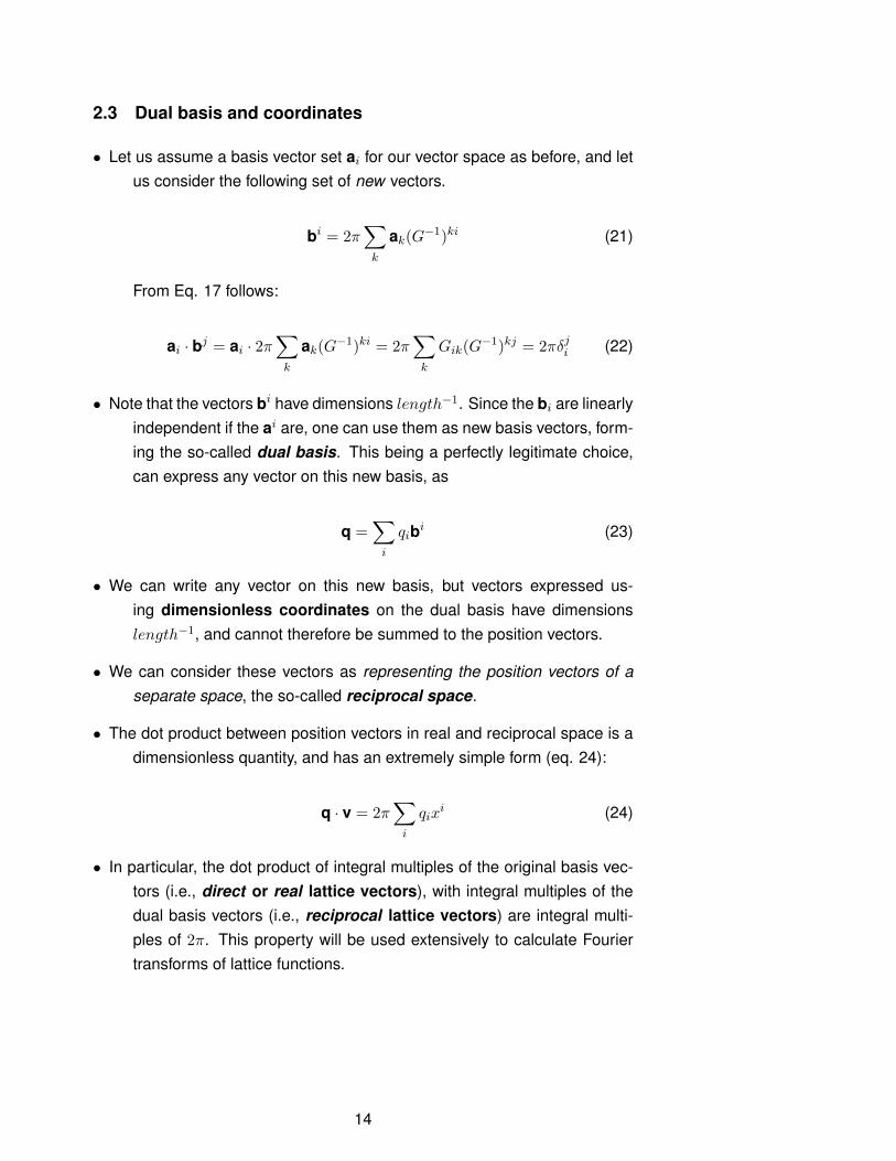
2.3 Dual basis and coordinates
• Let us assume a basis vector set ai for our vector space as before, and letus consider the following set of new vectors.
bi = 2π∑k
ak(G−1)ki (21)
From Eq. 17 follows:
ai · bj = ai · 2π∑k
ak(G−1)ki = 2π∑k
Gik(G−1)kj = 2πδji (22)
• Note that the vectors bi have dimensions length−1. Since the bi are linearlyindependent if the ai are, one can use them as new basis vectors, form-ing the so-called dual basis. This being a perfectly legitimate choice,can express any vector on this new basis, as
q =∑i
qibi (23)
• We can write any vector on this new basis, but vectors expressed us-ing dimensionless coordinates on the dual basis have dimensionslength−1, and cannot therefore be summed to the position vectors.
• We can consider these vectors as representing the position vectors of aseparate space, the so-called reciprocal space.
• The dot product between position vectors in real and reciprocal space is adimensionless quantity, and has an extremely simple form (eq. 24):
q · v = 2π∑i
qixi (24)
• In particular, the dot product of integral multiples of the original basis vec-tors (i.e., direct or real lattice vectors), with integral multiples of thedual basis vectors (i.e., reciprocal lattice vectors) are integral multi-ples of 2π. This property will be used extensively to calculate Fouriertransforms of lattice functions.
14
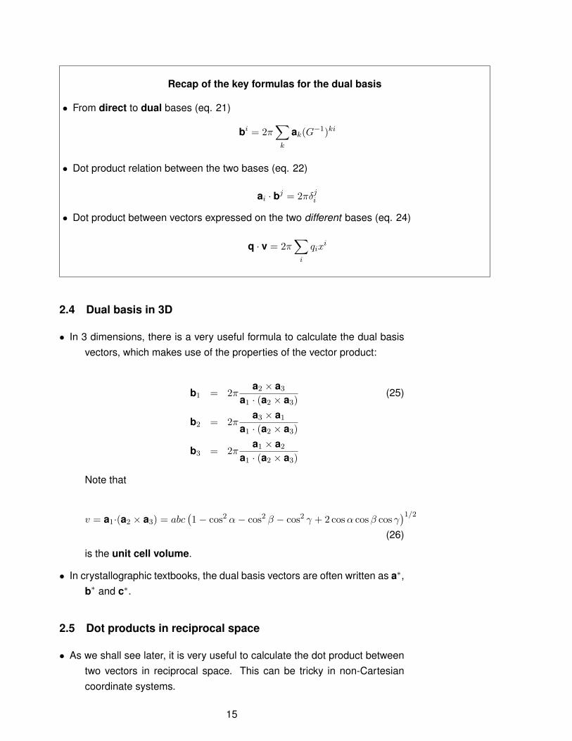
Recap of the key formulas for the dual basis
• From direct to dual bases (eq. 21)
bi = 2π∑k
ak(G−1)ki
• Dot product relation between the two bases (eq. 22)
ai · bj = 2πδji
• Dot product between vectors expressed on the two different bases (eq. 24)
q · v = 2π∑i
qixi
2.4 Dual basis in 3D
• In 3 dimensions, there is a very useful formula to calculate the dual basisvectors, which makes use of the properties of the vector product:
b1 = 2πa2 × a3
a1 · (a2 × a3)(25)
b2 = 2πa3 × a1
a1 · (a2 × a3)
b3 = 2πa1 × a2
a1 · (a2 × a3)
Note that
v = a1·(a2 × a3) = abc(1− cos2 α− cos2 β − cos2 γ + 2 cosα cosβ cos γ
)1/2(26)
is the unit cell volume.
• In crystallographic textbooks, the dual basis vectors are often written as a∗,b∗ and c∗.
2.5 Dot products in reciprocal space
• As we shall see later, it is very useful to calculate the dot product betweentwo vectors in reciprocal space. This can be tricky in non-Cartesiancoordinate systems.
15
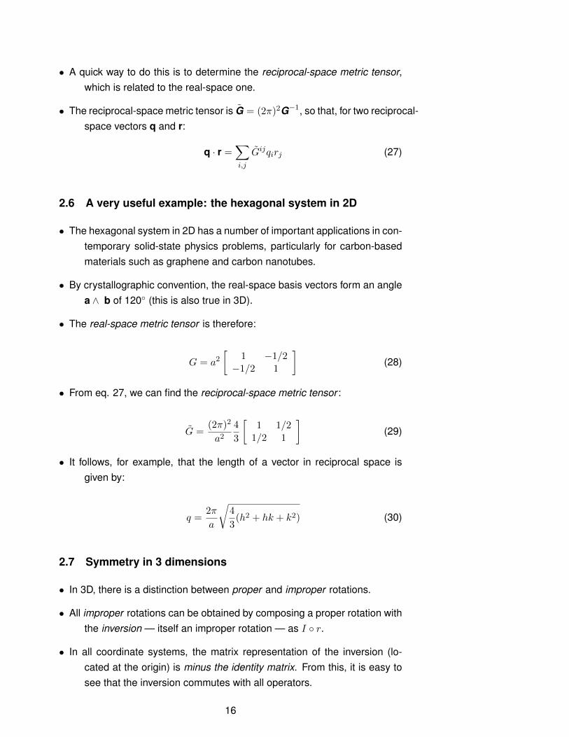
• A quick way to do this is to determine the reciprocal-space metric tensor,which is related to the real-space one.
• The reciprocal-space metric tensor is G̃ = (2π)2G−1, so that, for two reciprocal-space vectors q and r:
q · r =∑i,j
G̃ijqirj (27)
2.6 A very useful example: the hexagonal system in 2D
• The hexagonal system in 2D has a number of important applications in con-temporary solid-state physics problems, particularly for carbon-basedmaterials such as graphene and carbon nanotubes.
• By crystallographic convention, the real-space basis vectors form an anglea ∧ b of 120◦ (this is also true in 3D).
• The real-space metric tensor is therefore:
G = a2[
1 −1/2−1/2 1
](28)
• From eq. 27, we can find the reciprocal-space metric tensor :
G̃ =(2π)2
a24
3
[1 1/2
1/2 1
](29)
• It follows, for example, that the length of a vector in reciprocal space isgiven by:
q =2π
a
√4
3(h2 + hk + k2) (30)
2.7 Symmetry in 3 dimensions
• In 3D, there is a distinction between proper and improper rotations.
• All improper rotations can be obtained by composing a proper rotation withthe inversion — itself an improper rotation — as I ◦ r.
• In all coordinate systems, the matrix representation of the inversion (lo-cated at the origin) is minus the identity matrix. From this, it is easy tosee that the inversion commutes with all operators.
16

• I ◦ 2 = m⊥, so the mirror plane is the improper operator corresponding toa 2-fold rotation axis perpendicular to it.
• There are three other significant improper operators in 3D, known as roto-inversions. They are obtained by composition of an axis r of order
higher than two with the inversion, as I ◦r. These operators are 3̄ ( ),
4̄ ( ) and 6̄ ( ), and their action is summarized in Fig. 7. The sym-bols are chosen to emphasize the existence of another operator insidethe ”belly” of each new operator. Note that 3̄◦ 3̄◦ 3̄ = 3̄3 = I, and 3̄4 = 3,i.e., symmetries containing 3̄ also contain the inversion and the 3-foldrotation. Conversely, 4̄ and 6̄ do not automatically contain the inversion.In addition, symmetries containing both 4̄ (or 6̄) and I also contain 4 (or6).
-‐ +
-‐ +
+ -‐
+/-‐
+/-‐
+/-‐
+
-‐
+
-‐
Figure 7: Action of the 3̄ , 4̄ and 6̄ operators and their powers. The set of equivalent pointsforms a trigonal antiprism, a tetragonally-distorted tetrahedron and a trigonal prism, respec-tively. Points marked with ”+” and ”-” are above or below the projection plane, respectively.Positions marked with ”+/-” correspond to pairs of equivalent points above and below theplane.
• Glide planes in 3D have different symbols, depending on the orientation ofthe glide vector with respect to the plane of the projection (fig. 9).
• There is also a new type of operator, resulting from the compositions ofproper rotations with translation parallel to them. These are knownas screw axes.
• For an axis of order n, the nth power of a screw axis is a primitive trans-lation t . Therefore, the translation component must be m
n t, where m
is an integer. We can limit ourselves to m < n, all the other operatorsbeing composition with lattice translations. Roto-translation axes aretherefore indicated as nm, as in 21, 63 etc. (fig. 9).
17
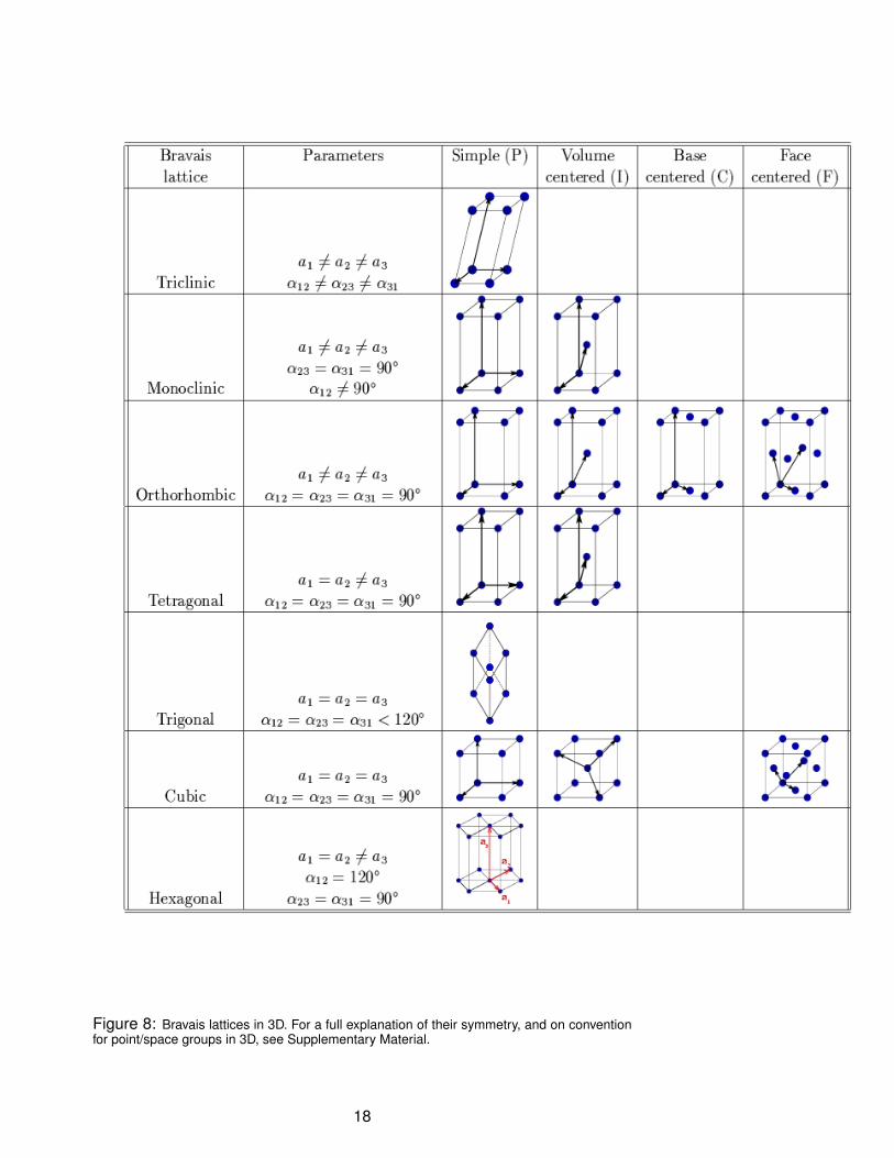
Figure 8: Bravais lattices in 3D. For a full explanation of their symmetry, and on conventionfor point/space groups in 3D, see Supplementary Material.
18

m a,b or c n e
31
32
41 43
42 61 65
62 64
63
2 21
d
18
38
2 3 4 6 m g
1 3 4 6
Figure 9: The most important graph symbols employed in the International Tables to de-scribe 3D space groups. Fraction next to the symmetry element indicate the height (z coordi-nate) with respect to the origin.
19
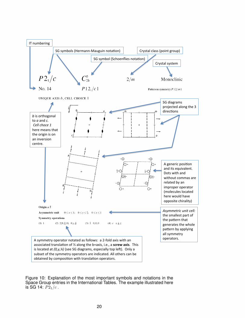
SG symbols (Hermann-‐Mauguin nota6on)
SG symbol (Schoenflies nota6on)
Crystal class (point group)
Crystal system
b is orthogonal to a and c. Cell choce 1 here means that the origin is on an inversion centre.
SG diagrams projected along the 3 direc6ons
A generic posi6on and its equivalent. Dots with and without commas are related by an improper operator (molecules located here would have opposite chirality)
Asymmetric unit cell: the smallest part of the paGern that generates the whole paGern by applying all symmetry operators. A symmetry operator notated as follows: a 2-‐fold axis with an
associated transla6on of ½ along the b=axis, i.e., a screw axis. This is located at (0,y,¼) (see SG diagrams, especially top leO). Only a subset of the symmetry operators are indicated. All others can be obtained by composi6on with transla6on operators.
IT numbering
Figure 10: Explanation of the most important symbols and notations in theSpace Group entries in the International Tables. The example illustrated hereis SG 14: P21/c .
20

Group generators
Refers to numbering of operators on previous page
Primi4ve transla4ons
4 pairs of equivalent inversion centres, not equivalent to centres in other pairs (not in the same class). They have their own dis4nct Wickoff leEer.
Equivalent posi4ons, obtained by applying the operators on the previous page (with numbering indicated). Reflects normal form of operators.
Reflec4on condi4ons for each class of reflec4ons. General: valid for all atoms (i.e., no h0l reflec4on will be observed unless l=2n; this is due to the c glide). Special: valid only for atoms located at corresponding posi4ons (leI side), i.e., atoms on inversion centres do not contribute unless k+l=2n
Figure 11: IT entry for SG 14: P21/c (page 2).
21

3 Lecture 3 — Fourier transform of periodic functions
3.1 Centring extinctions
• Reciprocal-space vectors are described as linear combinations of the re-ciprocal or dual basis vectors, (dimensions: length−1) with dimen-sionless coefficients.
• Reciprocal-lattice vectors (RLV ) are reciprocal space vectors with inte-gral components. These are known as the Miller indices and are usu-ally notated as hkl.
Dot products
• The dot product of real and reciprocal space vectors expressed in the usual coordinates is
q · v = 2π∑i
qivi (31)
• The dot product of real and reciprocal lattice vectors is:
- If a primitive basis is used to construct the dual basis, 2π times an integer for all qand v in the real and reciprocal lattice, respectively. In fact, as we just said, all thecomponents are integral in this case.
- If a conventional basis is used to construct the dual basis, 2π times an integer or asimple fraction of 2π. In fact the components of the centering vectors are fractional.
• Therefore, if a conventional real-space basis is used to construct the dual basis, only cer-tain reciprocal-lattice vectors will yield a 2πn dot product with all real-lattice vec-tors. These reciprocal-lattice vectors are exactly those generated by the correspond-ing primitive basis.
A conventional basis generates more RL vectors that a corresponding primitive basis.As we shall see, the “extra” points are not associated with any scattering intensity —
we will say that they are extinct by centering.
• Each non-primitive lattice type has centring extinctions, which can be ex-pressed in terms of the Miller indices hkl (see table 2).
• The non-exctinct reciprocal lattice points also form a lattice, which is natu-rally one of the 14 Bravais lattices. For each real-space Bravais lattice,tab. 3 lists the corresponding RL type.
22
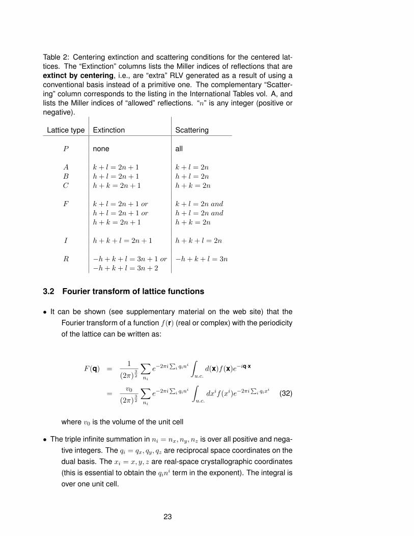
Table 2: Centering extinction and scattering conditions for the centered lat-tices. The “Extinction” columns lists the Miller indices of reflections that areextinct by centering, i.e., are “extra” RLV generated as a result of using aconventional basis instead of a primitive one. The complementary “Scatter-ing” column corresponds to the listing in the International Tables vol. A, andlists the Miller indices of “allowed” reflections. “n” is any integer (positive ornegative).
Lattice type Extinction Scattering
P none all
A k + l = 2n+ 1 k + l = 2nB h+ l = 2n+ 1 h+ l = 2nC h+ k = 2n+ 1 h+ k = 2n
F k + l = 2n+ 1 or k + l = 2n andh+ l = 2n+ 1 or h+ l = 2n andh+ k = 2n+ 1 h+ k = 2n
I h+ k + l = 2n+ 1 h+ k + l = 2n
R −h+ k + l = 3n+ 1 or −h+ k + l = 3n−h+ k + l = 3n+ 2
3.2 Fourier transform of lattice functions
• It can be shown (see supplementary material on the web site) that theFourier transform of a function f(r) (real or complex) with the periodicityof the lattice can be written as:
F (q) =1
(2π)32
∑ni
e−2πi∑
i qini
∫u.c.
d(x)f(x)e−iq·x
=v0
(2π)32
∑ni
e−2πi∑
i qini
∫u.c.
dxif(xi)e−2πi∑
i qixi
(32)
where v0 is the volume of the unit cell
• The triple infinite summation in ni = nx, ny, nz is over all positive and nega-tive integers. The qi = qx, qy, qz are reciprocal space coordinates on thedual basis. The xi = x, y, z are real-space crystallographic coordinates(this is essential to obtain the qini term in the exponent). The integral isover one unit cell.
23
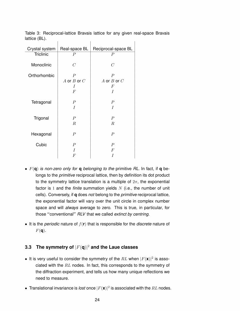
Table 3: Reciprocal-lattice Bravais lattice for any given real-space Bravaislattice (BL).
Crystal system Real-space BL Reciprocal-space BLTriclinic P P
Monoclinic C C
Orthorhombic P PA or B or C A or B or C
I FF I
Tetragonal P PI I
Trigonal P PR R
Hexagonal P P
Cubic P PI FF I
• F (q) is non-zero only for q belonging to the primitive RL. In fact, if q be-longs to the primitive reciprocal lattice, then by definition its dot productto the symmetry lattice translation is a multiple of 2π, the exponentialfactor is 1 and the finite summation yields N (i.e., the number of unitcells). Conversely, if q does not belong to the primitive reciprocal lattice,the exponential factor will vary over the unit circle in complex numberspace and will always average to zero. This is true, in particular, forthose “‘conventional”’ RLV that we called extinct by centring.
• It is the periodic nature of f(r) that is responsible for the discrete nature ofF (q).
3.3 The symmetry of |F (q)|2 and the Laue classes
• It is very useful to consider the symmetry of the RL when |F (x)|2 is asso-ciated with the RL nodes. In fact, this corresponds to the symmetry ofthe diffraction experiment, and tells us how many unique reflections weneed to measure.
• Translational invariance is lost once |F (x)|2 is associated with theRL nodes.
24
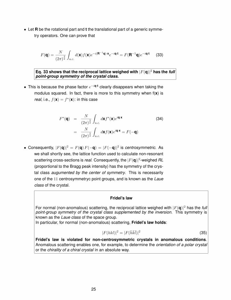
• Let R be the rotational part and t the translational part of a generic symme-try operators. One can prove that
F (q) =N
(2π)32
∫u.c.
d(x)f(x)e−i(R−1q)·xe−iq·t = F (R−1q)e−iq·t (33)
Eq. 33 shows that the reciprocal lattice weighed with |F (q)|2 has the fullpoint-group symmetry of the crystal class.
• This is because the phase factor e−iq·t clearly disappears when taking themodulus squared. In fact, there is more to this symmetry when f(x) isreal, i.e., f(x) = f∗(x): in this case
F ∗(q) =N
(2π)32
∫u.c.
dxf∗(x)eiq·x (34)
=N
(2π)32
∫u.c.
dxf(x)eiq·x = F (−q)
• Consequently, |F (q)|2 = F (q)F (−q) = |F (−q)|2 is centrosymmetric. Aswe shall shortly see, the lattice function used to calculate non-resonantscattering cross-sections is real. Consequently, the |F (q)|2-weighed RL(proportional to the Bragg peak intensity) has the symmetry of the crys-tal class augumented by the center of symmetry. This is necessarilyone of the 11 centrosymmetryc point groups, and is known as the Laueclass of the crystal.
Fridel’s law
For normal (non-anomalous) scattering, the reciprocal lattice weighed with |F (q)|2 has the fullpoint-group symmetry of the crystal class supplemented by the inversion. This symmetry isknown as the Laue class of the space group.In particular, for normal (non-anomalous) scattering, Fridel’s law holds:
|F (hkl)|2 = |F (h̄k̄l̄)|2 (35)
Fridel’s law is violated for non-centrosymmetric crystals in anomalous conditions.Anomalous scattering enables one, for example, to determine the orientation of a polar crystalor the chirality of a chiral crystal in an absolute way.
25
4 Lecture 4 — Brillouin zones and the symmetry ofthe band structure
• The electronic, vibrational and magnetic phenomena occurring in a crystalhave, overall, the same symmetry of the crystal.
• However, individual excitations (phonons, magnons, electrons, holes) breakmost of the symmetry, which is only restored because symmetry-equivalentexcitations also exist and have the same energy (and therefore popula-tion) at a given temperature.
• The wavevectors of these excitations are generic (non-RL) reciprocal-spacevectors.
• When these excitations are taken into account, one finds that inelastic scat-tering of light, X-rays or neutrons can occur. In general, the inelasticscattering will be outside the RL nodes.
• Various Wigner Seitz constructions 3 are employed to subdivide the recip-rocal space, for the purpose of:
� Classifying the wavevectors of the excitations. The Bloch theo-rem states that “crystal” wavevectors within the first Brillouin zone(first Wigner-Seitz cell) are sufficient for this purpose.
� Perform scattering experiments. In general, an excitation with wavevec-tor k (within the first Brillouin zone) will give rise to scattering at allpoints τ +k, where τ is a RLV . However, the observed scatteringintensity at these points will be different. The repeated Wigner-Seitz construction is particularly useful to map the “geography” ofscattering experiments.
� Construct Bloch wave functions (with crystal momentum withinthe first Brillouin zone) starting from free-electron wave-functions(with real wavevector k anywhere in reciprocal space). In partic-ular, apply degenerate perturbation theory to free-electron wave-functions with the same crystal wavevector. Here, the extendedWigner-Seitz construction is particularly useful, since free-electronwavefunctions within reciprocal space “fragments” belonging to thesame Brillouin zone form a continuous band of excitations.
• The different types of BZ constructions were already introduced last year.They are reviewed in the lecture and in the supplementary material onthe web site.
3A very good description of the Wigner-Seitz and Brillouin constructions can be found in [?].See also the Supplementary Material for a summary of the procedure.
26

k
Figure 12: A set of typical 1-dimensional electronic dispersion curves in thereduced/repeated zone scheme.
4.1 Symmetry of the electronic band structure
• We will here consider the case of electronic wavefunctions, but it isimportant to state that almost identical considerations can be appliedto other wave-like excitations in crystals, such as phonons and spinwaves (magnons).
• Bloch theorem: in the presence of a periodic potential, electronic wave-functions in a crystal have the Bloch form:
ψk(r) = eik·ruk(r) (36)
where uk(r) has the periodicity of the crystal. We also recall that thecrystal wavevector k can be limited to the first Brillouin zone (BZ). Infact, a function ψk′(r) = eik
′·ruk′(r) with k′ outside the first BZ can berewritten as
ψk′(r) = eik·r[eiτ ·ruk′(r)
](37)
where k′ = τ+k, k is within the 1st BZ and τ is a reciprocal lattice vector(RLV ). Note that the function in square brackets has the periodicity ofthe crystal, so that eq. 37 is in the Bloch form.
27
• The application of the Bloch theorem to 1-dimensional (1D) electronic wave-functions, using either the nearly-free electron approximation or thetight-binding approximation leads to the typical set of electronic disper-sion curves (E vs. k relations) shown in fig. 12. We draw attention tothree important features of these curves:
• Properties of the electronic dispersions in 1D
� They are symmetrical (i.e., even) around the origin.
� The left and right zone boundary points differ by the RLV 2π/a, andare also related by symmetry.
� The slope of the dispersions is zero both at the zone centre and atthe zone boundary. We recall that the slope (or more generally thegradient of the dispersion is related to the group velocity of thewavefunctions in band n by:
vn(k) =1
~∂En(k)
∂k(38)
• Properties of the electronic dispersions in 2D and 3D
� They have the full Laue (point-group) symmetry of the crystal. Thisapplies to both energies (scalar quantities) and velocities (vectorquantities)
� Zone edge centre (2D) or face centre (3D) points on opposite sidesof the origin differ by a RLV and are also related by inversion sym-metry.
� Otherwise, zone boundary points that are related by symmetry do notnot necessarily differ by a RLV .
� Zone boundary points that differ by aRLV are not necessarily relatedby symmetry.
� Group velocities are zero at zone centre, edge centre (2D) or facecentre (3D) points.
� Some components of the group velocities are (usually) zero at zoneboundary points (very low-symmetry cases are an exception —see below).
� Group velocities directions are constrained by symmetry on symme-try elements such as mirror planes and rotation axes.
• The dispersion of the band structure, En(k), has the Laue symmetry of thecrystal. This is because:
28
� En(k) is a macroscopic observable (it can be mapped, for example,by Angle Resolved Photoemission Spectroscopy — ARPES) andany macroscopic observable property of the crystal must have atleast the point-group symmetry of the crystal (Neumann’s principle— see later).
� If the Bloch wavefunction ψk = eik·ruk(r) is an eigenstate of theSchroedinger equation
[− ~2
2m∇2 + U(r)
]ψk = Ekψk (39)
then ψ†k = e−ik·ru†k(r) is a solution of the same Schroedinger equa-tion with the same eigenvalue (this is always the case if the poten-tial is a real function). ψ†k has crystal momentum −k. Therefore,the energy dispersion surfaces (and the group velocities) must beinversion-symmetric even if the crystal is not.
4.2 Symmetry properties of the group velocity
• The group velocity at two points related by inversion in the BZ must beopposite.
• For points related by a mirror plane or a 2-fold axis, the components of thegroup velocity parallel and perpendicular to the plane or axis must beequal or opposite, respectively.
• Similar constraints apply to points related by higher-order axes — in partic-ular, the components of the group velocity parallel to the axis must beequal.
• Since eik·ruk(r) = ei(k+τ)·r{e−τ ·ruk(r)} and the latter has crystal momen-tum k + τ , Ek must be the same at points on opposite faces across theBrillouin zone (BZ), separated by τ .
• If the band dispersion Ek is smooth through the zone boundary, then thegradient of Ek (and therefore vn(k)) must be the same at points onopposite faces across the Brillouin zone (BZ), separated by τ . 4
4This leaves the possibility open for cases in which vn(k) jumps discontinuosly across theBZ boundary and is therefore not well defined exactly at the boundary. This can only happenif bands with different symmetries cross exactly at the BZ boundary.
29
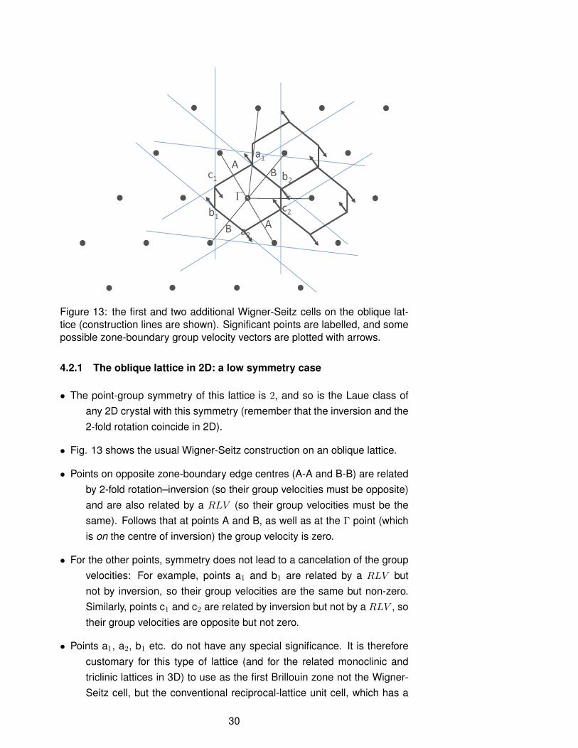
Figure 13: the first and two additional Wigner-Seitz cells on the oblique lat-tice (construction lines are shown). Significant points are labelled, and somepossible zone-boundary group velocity vectors are plotted with arrows.
4.2.1 The oblique lattice in 2D: a low symmetry case
• The point-group symmetry of this lattice is 2, and so is the Laue class ofany 2D crystal with this symmetry (remember that the inversion and the2-fold rotation coincide in 2D).
• Fig. 13 shows the usual Wigner-Seitz construction on an oblique lattice.
• Points on opposite zone-boundary edge centres (A-A and B-B) are relatedby 2-fold rotation–inversion (so their group velocities must be opposite)and are also related by a RLV (so their group velocities must be thesame). Follows that at points A and B, as well as at the Γ point (whichis on the centre of inversion) the group velocity is zero.
• For the other points, symmetry does not lead to a cancelation of the groupvelocities: For example, points a1 and b1 are related by a RLV butnot by inversion, so their group velocities are the same but non-zero.Similarly, points c1 and c2 are related by inversion but not by a RLV , sotheir group velocities are opposite but not zero.
• Points a1, a2, b1 etc. do not have any special significance. It is thereforecustomary for this type of lattice (and for the related monoclinic andtriclinic lattices in 3D) to use as the first Brillouin zone not the Wigner-Seitz cell, but the conventional reciprocal-lattice unit cell, which has a
30
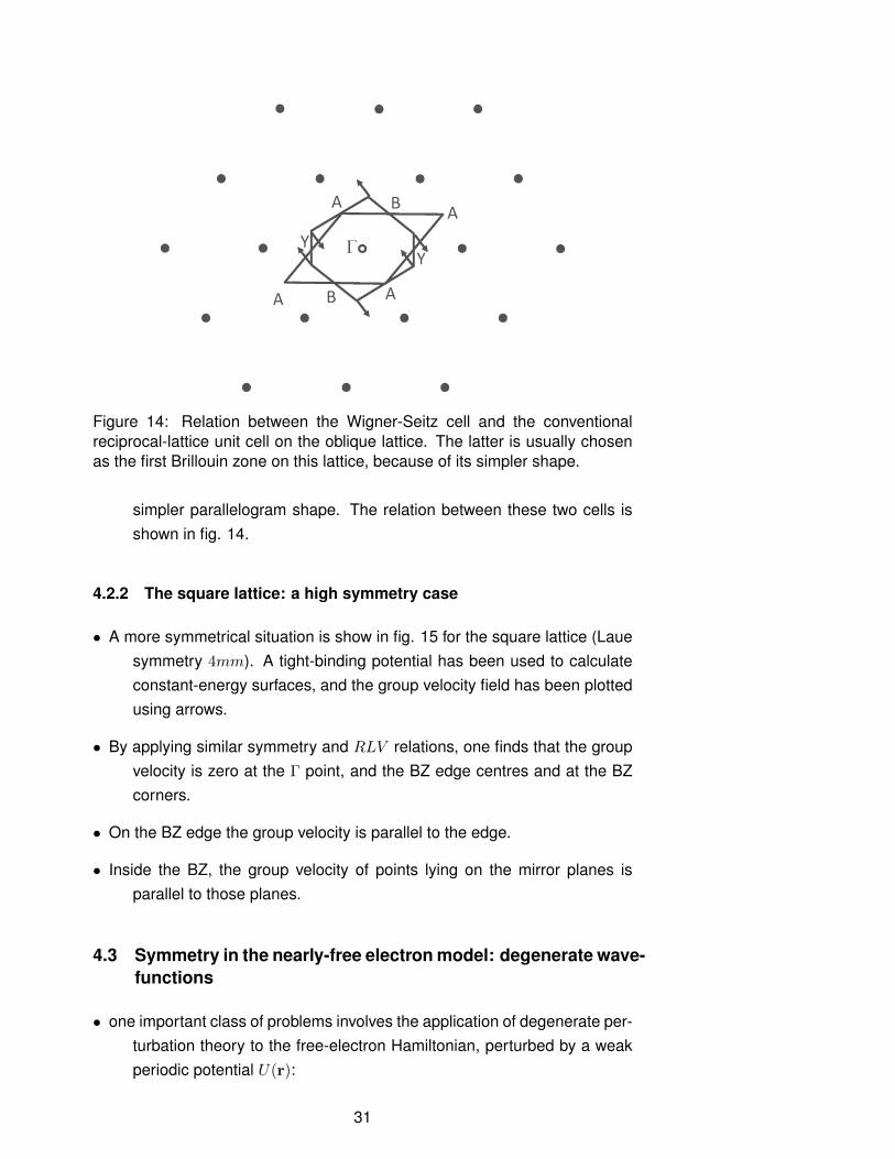
Figure 14: Relation between the Wigner-Seitz cell and the conventionalreciprocal-lattice unit cell on the oblique lattice. The latter is usually chosenas the first Brillouin zone on this lattice, because of its simpler shape.
simpler parallelogram shape. The relation between these two cells isshown in fig. 14.
4.2.2 The square lattice: a high symmetry case
• A more symmetrical situation is show in fig. 15 for the square lattice (Lauesymmetry 4mm). A tight-binding potential has been used to calculateconstant-energy surfaces, and the group velocity field has been plottedusing arrows.
• By applying similar symmetry and RLV relations, one finds that the groupvelocity is zero at the Γ point, and the BZ edge centres and at the BZcorners.
• On the BZ edge the group velocity is parallel to the edge.
• Inside the BZ, the group velocity of points lying on the mirror planes isparallel to those planes.
4.3 Symmetry in the nearly-free electron model: degenerate wave-functions
• one important class of problems involves the application of degenerate per-turbation theory to the free-electron Hamiltonian, perturbed by a weakperiodic potential U(r):
31

Figure 15: Constant-energy surfaces and group velocity field on a squarelattice, shown in the repeated zone scheme. The energy surfaces have beencalculated using a tight-binding potential.
32

H = − ~2
2m∇2 + U(r) (40)
• Since the potential is periodic, only degenerate points related by a RLV
are allowed to “interact” in degenerate perturbation theory and give riseto non-zero matrix elements.
• The 1D case is very simple:
� Points inside the BZ have a degeneracy of one and correspond totravelling waves.
� Points at the zone boundary have a degeneracy of two, since k = π/a
and therefore k − (−k) = 2π/a is a RLV . The perturbed solutionsare standing wave, and have a null group velocity, as we have seen(fig. 12).
• The situation is 2D and 3D is rather different, and this is where symmetrycan help. In a typical problem, one would be asked to calculate theenergy gaps and the level structure at a particular point, usually but notnecessarily at the first Brillouin zone boundary.
• The first step in the solution involves determining which and how many de-generate free-electron wavefunctions with momenta differing by a RLVhave a crystal wavevector at that particular point of the BZ.
• Symmetry can be very helpful in setting up this initial step, particularly if thesymmetry is sufficiently high. For the detailed calculation of the gaps,we will defer to the “band structure” part of the C3 course.
Nearly-free electron degenerate wavefunctions
• Draw a circle centred at the Γ point and passing through the BZ point you are asked toconsider (either in the first or in higher BZ — see fig. 16). Points on this circle correspondto free-electron wavefunctions having the same energy.
• Mark all the points on the circle that are symmetry-equivalent to your BZ point.
• Among these, group together the points that are related by a RLV . These points representthe degenerate multiplet you need to apply degenerate perturbation theory.
• Write the free-electron wavefunctions of your degenerate multiplet in Bloch form. You will findthat all the wavefunctions in each multiplet have the same crystal momentum. Functionsin different multiplets have symmetry-related crystal momenta.
• This construction is shown in fig. 16 in the case of the square lattice (pointgroup 4mm) for boundary points between different Brillouin zones. Onecan see that:
33
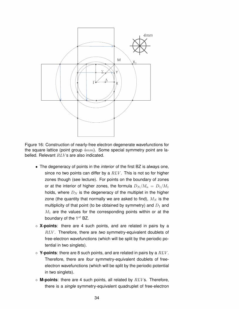
Figure 16: Construction of nearly-free electron degenerate wavefunctions forthe square lattice (point group 4mm). Some special symmetry point are la-belled. Relevant RLV s are also indicated.
• The degeneracy of points in the interior of the first BZ is always one,since no two points can differ by a RLV . This is not so for higherzones though (see lecture). For points on the boundary of zonesor at the interior of higher zones, the formula DN/Mn = D1/M1
holds, where DN is the degeneracy of the multiplet in the higherzone (the quantity that normally we are asked to find), MN is themultiplicity of that point (to be obtained by symmetry) and D1 andM1 are the values for the corresponding points within or at theboundary of the 1st BZ.
� X-points: there are 4 such points, and are related in pairs by aRLV . Therefore, there are two symmetry-equivalent doublets offree-electron wavefunctions (which will be split by the periodic po-tential in two singlets).
� Y-points: there are 8 such points, and are related in pairs by a RLV .Therefore, there are four symmetry-equivalent doublets of free-electron wavefunctions (which will be split by the periodic potentialin two singlets).
� M-points: there are 4 such points, all related by RLV s. Therefore,there is a single symmetry-equivalent quadruplet of free-electron
34

wavefunctions (which will be split by the periodic potential in twosinglets and a doublet).
� X2-points: these are X-point in a higher Brillouin zone. There are 8such points, related by RLV s in groups of four. Therefore, thereare two symmetry-equivalent quadruplets of free-electron wave-functions (each will be split by the periodic potential in two singletsand a doublet). These two quadruplets will be brought back above(in energy) the previous two doublets in the reduced-zone scheme.
35