Crystal Structure and DynamicsPaolo G. Radaelli, Michaelmas Term 2014

Part 2: Scattering theory and experimentsLectures 6-8

Web Site:http://www2.physics.ox.ac.uk/students/course-materials/c3-condensed-matter-major-option

Bibliography B.E. Warren, X-ray diffraction Dover Publications, Inc., New York, 2nd Ed. 1990. is a rather

old book with a very dated notation, but somehow I always find myself going back to it.Some of the explanations are very clear.

G.L. Squires Introduction to thermal neutron scattering Dover Publications, Cambridge, NewYork, 1978is a classic introductory book, and has all the basic derivations of nuclear andmagnetic cross sections.

John D. Jackson ‘Classical Electrodynamics John Wiley & sons, New York, Chichister, Bris-bane, Toronto, Singapore, (1975). This book provides detailed derivation of the classicalX-ray scattering cross section. It is a very complete compendium of electrodynamics,although not always easy to digest...

Stephen W. Lovesey,Theory of neutron scattering from condensed matter , Oxford SciencePublications, Clarendon Press, Oxford (1984) — in 2 volumes. This is “the” texbook onthe theory of neutron scattering and related matters.

E. H. Kisi Applications of neutron powder diffractionOxford University Press, Oxford, NewYork, 2008 is a more recent book on neutron diffraction, focussing on the powder method.

Andre Authier Dynamical Theory of X-ray Diffraction, International Union of Crystallography,Oxford University Press (Oxford, New York), 2001. This is a very complete book on thedynamical theory of X-ray scattering. It has a good historical introduction and some simpleexplanations of the phenomena.

P.J. Grundy & G.A. Jones Electron Microscopy in the Study of Materials, (Edward ArnoldLtd. London: UK, 1976). A handy booklet on electron microscopy, a bit old but still usefulto understand how dislocations can be imaged.

S.J.L. Billinge & M.F. Thorpe Local structure from diffraction, Kluwer Academic PublishersNew York, Boston, Dordrecht, London, Moscow, 2002. A good collection of articles ondiffuse scattering and scattering from disordered materials.

1

Contents

1 Lecture 6 — Scattering from individual atoms and spins 31.1 Thomson scattering of X-rays from a single electron . . . . . . . . . . . . . . . . 31.2 Thomson scattering from many quasi-free electrons . . . . . . . . . . . . . . . . 51.3 X-ray scattering from bound electrons — anomalous scattering . . . . . . . . . . 71.4 Thermal neutron scattering from atoms and spins . . . . . . . . . . . . . . . . . . 8

2 Lecture 7 - Scattering from crystals 112.1 Cross section for a “small” perfect single crystal . . . . . . . . . . . . . . . . . . . 112.2 Laue and Bragg equations . . . . . . . . . . . . . . . . . . . . . . . . . . . . . . . 142.3 The effect of atomic vibrations — the Debye-Waller factor . . . . . . . . . . . . . 152.4 Finite size effects . . . . . . . . . . . . . . . . . . . . . . . . . . . . . . . . . . . . 17

3 Lecture 8 - Diffraction experiments and data analysis 193.1 Geometries for diffraction experiments - single crystal diffraction . . . . . . . . . 19

3.1.1 Scattering triangles for elastic scattering and the Ewald construction . . . 193.2 Scattering triangles for inelastic scattering . . . . . . . . . . . . . . . . . . . . . . 203.3 Powder diffraction and the Debye-Scherrer cones . . . . . . . . . . . . . . . . . . 223.4 Integrated Intensities . . . . . . . . . . . . . . . . . . . . . . . . . . . . . . . . . . 223.5 Structural solution from diffraction data . . . . . . . . . . . . . . . . . . . . . . . . 24

3.5.1 The phase problem . . . . . . . . . . . . . . . . . . . . . . . . . . . . . . 243.5.2 The Patterson method . . . . . . . . . . . . . . . . . . . . . . . . . . . . . 253.5.3 Structural optimisation: least-square refinements . . . . . . . . . . . . . . 26

2

1 Lecture 6 — Scattering from individual atoms andspins

In order to extract information about the atomic structure of a crystal, liquidor glass by diffraction, the wavelength of the probe must be compara-ble or smaller than the interatomic distances, which are typically a fewAngstroms (10−10 m, or 10−1 nm). Tab. 1 illustrates the typical wavelengthsand energies employed for X-ray, neutron and electron diffraction.

Table 1: Typical wavelenghts and energies employed for X-ray, neutron andelectron diffraction. For electromagnetic radiation, E = hc/λ, with hc = 12.4

KeV · A; for a non-relativistic particle beam, E = 2π2~2mλ2

=, where 2π2~2m = 82

meV · A2 for neutrons and 150 eV · A2 for electrons. A typical TransmissionElectron Microscope (TEM) can operate at 200 KV raising the electron ve-locity to 70 % of the speed of light, and some state-of-the-art microscopescan reach the MV range; therefore, relativistic effects need to be taken intoaccount in converting between energy and wavelength.

λ E

X-rays 0.1–6 A 2–150 KeVneutrons 0.3–10 A 1–1000 meVelectrons 0.02–3 A 20 eV–200 KeV

Powerful X-ray, neutron and electron sources and diffraction instruments ateavailable to the experimentalists. For more detail, see the SupplementaryMaterial.

1.1 Thomson scattering of X-rays from a single electron

• Bragg diffraction of X-rays is primarily due to the scattering from elec-trons bound to the atoms of the crystal structure. It is generally a verygood approximation to employ the so-called Thomson formula (from J.J.Thomson, Nobel Prize 1906) to calculate the relevant scattering ampli-tudes and cross sections. This is a bit of a paradox, since the Thomsonformula assumes free electrons1, but the agreement with experimentsin nonetheless very good. The Thomson formula is valid in the non-relativistic limit (velocity of the particle << c).

• By using classical electrodynamics, we can calculate the time-dependentamplitude of the electric field generated at a distanceR from an electronthat has been accelerated by an electromagnetic plane wave.

1A description of the scattering process beyond the free electron approximation is con-tained in the Supplementary Material.

3

• If the time-dependent electric field at the position of the electron is

E = εE0e−iωt (1)

and the incident polarisation (see fig. 1) is

ε = cos ξ εσ + sin ξ επ (2)

then2

E(R, t) = −r0E0ei(kR−ωt)

R

[cos ξ ε′σ + sin ξ cos γ ε′π

](3)

where

r0 =e2

4πε0mc2= 2.82× 10−15 m (4)

is the classical radius of the electron.

• The scattering angle γ is the angle between the incident and scatteredwavevector (this angle is also known, by longstanding diffraction con-vention, as 2θ). Based on eq. 3, we can make the following observa-tions:

Figure 1: Diagram illustrating the conventional σ and π reference directionsfor the incident and scattered polarisation. Note that εσ · ε′σ = 1 always.Conversely, επ·ε′π = cos γ depends on the scattering angle γ, and vanishesfor γ = π/2.

• A plane wave impinging on a quasi-free charge produces a scattered spher-

ical waveei(kR−ωt)

R, with an amplitude that in general depends on the

scattering angle γ.2See Supplementary Material for a complete derivation.

4

• If the incident wave is σ-polarised, the scattered wave is σ′-polarised, andhas amplitude r0

R E0.

• If the incident wave is π-polarised, the scattered wave is π′-polarised, andhas amplitude r0

R E0 cos γ.

• The intensity of the scattered wave is zero for scattering of π polarisationat 90.

• The scattered wave has a phase shift of π upon scattering (minus sign).

• For generic incident polarisation, the scattering amplitude (amplitude of thespherical wave) in each scattered polarisation can be written as:

A = r0[ε · ε′] (5)

• The cross section is defined as the average power radiated per unit solidangle divided by the average incident power per unit area (power flux,Φ)

• For an unpolarised X-ray beam, all the angles ξ are equally represented(i.e., there will be photons with all polarisations). The cross section inthis case is

dσ

dΩ= r20

[1 + cos2 γ

2

](6)

1.2 Thomson scattering from many quasi-free electrons

• When many electrons are inclose proximity to each other, the sphericalwaves emitted by them will interfere.

• The combined effect of these waves can be calculated in the following ap-proximations:

The amplitude of the motion of the electrons is much smaller than thewavelength.

The distance at which the process is observed is also much largerthan the distance between electrons (Fraunhofer diffraction or far-field limit).

The distribution of electrons can be considered continuous, with num-ber density ρ(x) [electrons/m3].

5

With these approximations, which are always obeyed for the electroncloud around an atom and reasonable values of the electric field)

E(R, t) = −r0E0ei(kR−ωt)

R

[cos ξ ε′σ + sin ξ cos γ ε′π

] ∫ρ(x)e−iq·xdx

(7)

• The vector q = kf − ki is the scattering vector and ki and kf are theincident and scattered wavevectors.

• Note the important formula, valid for elastic scattering (we recall that γ =

2θ):

q = |q| = 4π sin θ

λ(8)

Eq. 8 is illustrated graphically in fig. 2

Figure 2: Scattering triangle for elastic scattering.

• The integral

f(q) =

∫ρ(x)e−iq·xdx (9)

is known as the atomic scattering factor or form factor.

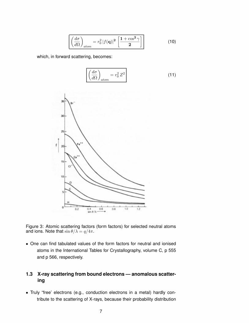
We have arrived here at an important result: the scattering amplitude for many quasi-freeelectrons is proportional to the Fourier transform of the charge density. Note that theintegral for q = 0 is the total charge, which for an atom is the atomic number Z (fig. 3).

A key fact to remember: the more spread out the charge is around the atom, the fasterf(q) will decay at high q.

High q ≡ high scattering angles, short wavelengths.

• The cross sections are obtained in the same way as for a single charge —for instance, the unpolarised cross section for an atom is:

6

(dσ

dΩ

)atom

= r20 |f(q)|2[1 + cos2 γ

2

](10)

which, in forward scattering, becomes:

(dσ

dΩ

)atom

= r20 Z2 (11)

Figure 3: Atomic scattering factors (form factors) for selected neutral atomsand ions. Note that sin θ/λ = q/4π.

• One can find tabulated values of the form factors for neutral and ionisedatoms in the International Tables for Crystallography, volume C, p 555and p 566, respectively.

1.3 X-ray scattering from bound electrons — anomalous scatter-ing

• Truly “free’ electrons (e.g., conduction electrons in a metal) hardly con-tribute to the scattering of X-rays, because their probability distribution

7

extends a long way throughout the crystal, and, from eq. 9, the formfactor decays very rapidly away from forward scattering (fig. 3).

• The largest contribution to X-ray scattering from atoms is given by “core”electrons, which are close to the nucleus and have slowly decaying fromfactors — but these electrons are certainly not free!

• There are large departures from the Thomson scattering formula near atomicresonances, where the energy of the photon is just sufficient to eject anelectron from a core state into the continuum. Away from resonances,the Thomson formula can be corrected to a very good approximation byreplacing the form factor by the complex quantity

f(q) = fThom(q) + f ′(~ω) + if ′′(~ω) (12)

where the so-called anomalous terms, f ′ and f ′′, away from atomicresonances do not depend on q and are weak functions of the photonenergy 3.

It can be shown, as a consequence of the so-called optical theorem, that the imaginarypart of the scattering factor is proportional to the linear absorption coefficient due to thephotoelectric effect.

f ′′(~ω) =ω

4πr0cNaµ (13)

where Na is the number of atoms per unit volume, and the other symbols have the usualmeaning. The quantity µ is the linear absorption coefficient, defined as:

I = I0e−µL (14)

1.4 Thermal neutron scattering from atoms and spins

• As in the case of X-rays, the neutron scattering process generates a spher-ical wave, the squared amplitude of which is proportional to the crosssection.

• Thermal neutrons, with energies in the meV range, are commonly usedto probe condensed matter. Their properties can be summarised asfollows:

Free neutrons are unstable, with half-life τ = 10.6 min. (β-decay)3See Supplementary Material for more details about resonant X-ray scattering.

8

Neutrons bound in nuclei are (generally) stable.

Mass: 1.67492729(28)× 10−27 kg

Electric dipole moment D < 10−25 (e cm)

Spin: s = 12 — neutrons are fermions.

Magnetic dipole moment: µ = −1.9130418 µN , where µN = e~2mp

=

5.05078324(13)× 10−27 JT−1 is the nuclear magneton.

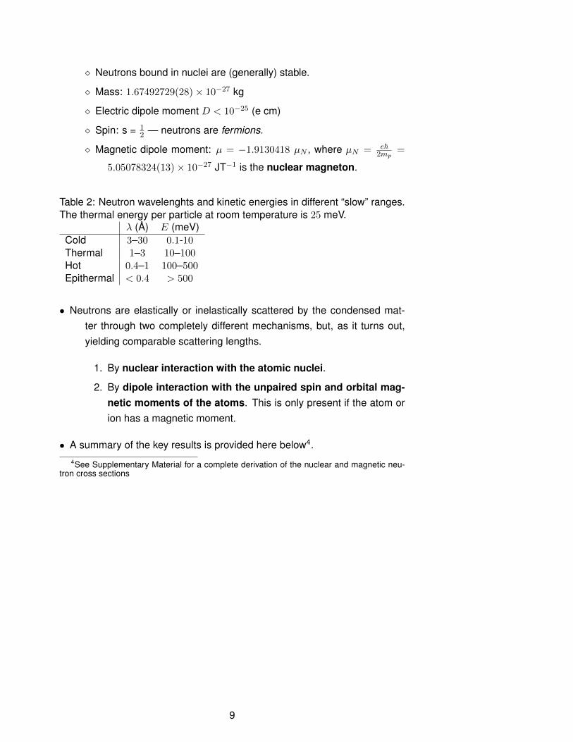
Table 2: Neutron wavelenghts and kinetic energies in different “slow” ranges.The thermal energy per particle at room temperature is 25 meV.

λ (A) E (meV)Cold 3–30 0.1-10Thermal 1–3 10–100Hot 0.4–1 100–500Epithermal < 0.4 > 500

• Neutrons are elastically or inelastically scattered by the condensed mat-ter through two completely different mechanisms, but, as it turns out,yielding comparable scattering lengths.

1. By nuclear interaction with the atomic nuclei.

2. By dipole interaction with the unpaired spin and orbital mag-netic moments of the atoms. This is only present if the atom orion has a magnetic moment.

• A summary of the key results is provided here below4.4See Supplementary Material for a complete derivation of the nuclear and magnetic neu-

tron cross sections

9

Neutron-nuclear interaction

• The neutron-nuclear interaction is isotope and elements specific, and depends on themutual orientation of the neutron and the nuclear spin.

• As far as neutron crystallography is concerned, the key parameter is the scattering ampli-tude averaged over the nuclear spin states, known as the coherent scattering ampli-tude.

• The neutron nuclear coherent scattering amplitude is independent on q — it carries noform factor, and is therefore expressed by a single number, known as the Fermi length.

• Fermi lengths can be positive or negative, depending on whether the neutron-nuclearinteraction is attractive or repulsive. For typical nuclei, they are of the order of a few fm(10−15 m) (see fig 4), which means that they are comparable to the classical electronradius. However, atoms have a single nucleus and many electrons, so X-ray scatteringcross sections in the forward direction are typically much larger than neutron cross sec-tions (X-ray cross sections decay at high q due to the form factor).

• Fermi lengths do not vary in a systematic way across the periodic table (fig 4), which meansthat with respect to X-rays, neutrons are uniquely sensitive to some light elements— notably oxygen. The different scattering lengths of different isotopes is also widelyexploited in the so-called contrast variation techniques.

Figure 4: Variation of the Fermi length as a function of atomic weight.

10

Neutron-magnetic interaction

• When the scatterer carries a magnetic moment, in addition to the normal nuclear interaction,neutron are also scattered by dipole-dipole interaction from the magnetic moment of theatom.

• Magnetic scattering of neutrons is governed by the following vector scattering amplitude.

An = γNr0fm(q)M⊥ (15)

where γN is the neutron gyromagnetic ratio (−1.9130418), r0 is the familiar classical elec-tron radius and M⊥ is the projection of the atomic magnetic moment perpendicularto the wavevector transfer q, and is expressed in Bohr magnetons.

• The quantity fm(q) is known as the neutron magnetic form factor, and is normalised so thatfm(0) = 1. It is similar to the X-ray form factor, except for the fact that it only include themore extended density of unpaired electrons. Therefore magnetic neutron scatteringdecays very rapidly at high q.

• From eq. 15 one can obtain a number of cross sections, accounting for the different ori-entations of the neutron spin with respect to the atomic magnetic moment (neutron po-larisation). The most important cross section is the unpolarised neutron cross section(averaged over all the possible neutron polarisations), which, for a single atom, is:

dσ

dΩ= γ2Nr

20f

2m(q)|M⊥|2 = γ2Nr

20f

2m(q)M2 sin2 α (16)

where α is the angle between M and q. Note that the cross section is zero if q isparallel to M.

• Typical magnetic moments for atoms and ions are a few Bohr magnetons. Therefore, fromeq. 16, one finds that neutron nuclear and magnetic scattering cross sections aretypically comparable in magnitude for magnetic atoms.

11

2 Lecture 7 - Scattering from crystals

2.1 Cross section for a “small” perfect single crystal

• We want to calculate the scattering cross section from a “small” single crys-tal. Here, “small” means that we can ignore multiple scattering events.We still consider the crystal as perfectly periodic.

• We will employ the same approximations that we have used for the scat-tering from many quasi-free electrons (the far-field approximation is notobeyed in some relevant cases, but we will not concern ourselves withthem).

• We will consider the case of X-rays, but the calculation is analogous forneutrons. The scattering amplitude in each final polarisation directionis obtained by integrating over the whole crystal (instead that around anatom, as for eq. 7):

A(q) = r0∫Crystal drρ(r)e−iq·r [ε · ε′] (17)

• We can exploit the fact that the charge density is periodic, so that, if ri is alattice translation and x is restricted to the unit cell containing the origin:

ρ(r) = ρ(ri + x) = ρ(x) (18)

whence the scattering amplitude becomes

A(q) = r0∑i

∫UnitCell

dxρ(x)e−iq·(ri+x)[ε · ε′

]= r0

∑i

e−iq·ri∫UnitCell

dxρ(x)e−iq·x[ε · ε′

](19)

where the summation runs over all the unit cells in the crystal. Theexpression

F (q) = r0

∫UnitCell

dxρ(x)e−iq·x (20)

is known as the structure factor. Note the close analogy with eq. 32,Part I.

The structure factor is proportional to the Fourier transform of the charge density (or,more in general, scattering density) integrated over the unit cell.

12

• If the electron density ρ(r) is a superposition of atomic-like electron densi-ties (i.e., a series of δ functions), F (q) can be written as

F (q) = r0∑n

fn(q)e−iq·xn (21)

where the sum runs over all the atoms in the unit cell and fn(q) are theform factors of each species and xn are their positions within the unitcell.

• We can now calculate the cross section:

dσ

dΩ= A(q)A∗(q) =

∑j

∑i

e−iq·(ri−rj)

|F(q)|2[ε · ε′

]2 (22)

• We now introduce the fact that the double summation in parentheses canbe consider as running over an infinite lattice. Consequently, all thesummations over i labelled by rj are the same (they only differ by a shiftin origin), and the summation over j can be replaced by multiplicationby Nc — the number of unit cells in the crystal (→∞).

• The remaining single summation is only non-zero when q is a RL vector. Ifq is restricted to the first Brillouin zone, we can write:

δ(q) =1

(2π)3

∫dxe−iq·x ' v0

(2π)3

∑i

e−iq·ri (23)

where v0 is the unit cell volume. For an unrestricted q, the same ex-pression holds with the left-hand member replaced by a sum of deltafunctions centred at all reciprocal lattice nodes, indicated with τ in theremainder. With this, we can write the final expression for the crosssection:

dσ

dΩ= Nc

(2π)3

v0

∑τ

δ(q− τ )|F (τ )|2[ε · ε′

]2 (24)

• The term [ε · ε′]2 needs to be averaged over all this incident and scatteredpolarisations, yielding a polarisation factor P(γ), which depends onthe experimental setting. For example, for an unpolarised incident beamand no polarisation analysis:

13

P(γ) =

[1 + cos2 γ

2

]unpolarised beam (25)

• The final general expression for the average cross section is:

dσ

dΩ= Nc

(2π)3

v0

∑τ

δ(q− τ )|F (τ )|2P(γ) (26)

Let’s recap the key points to remember:

The cross section is proportional to the number of unit cells in the crystal. The biggerthe crystal, the more photons or particles will be scattered. We can clearly see thatthis result must involve an approximation: the scattered intensity must reach a limitwhen all the particles in the beam are scattered.

The cross section is proportional to the squared modulus of the structure factor (nosurprises here — you should have learned this last year).

Scattering only occurs at the nodes of the RL. For a perfect, infinite crystal, this is inthe form of delta functions.

The cross section contains the unit-cell volume in the denominator. This is necessaryfor dimensional reasons, but it could perhaps cause surprise. After all, we couldarbitrarily decide to double the size of the unit cell by introducing a “basis”. Theanswer is, naturally, that the |F (τ )|2 term exactly compensates for this.

• The limitations of the small crystal approximation can be overcome by com-plete description of the scattering process, including multiple scattering,in what is known as dynamical theory of diffraction (see extendedversion of the notes for a very short introduction).

2.2 Laue and Bragg equations

• The δ function in eq. 24 expresses the fact that the cross section is zerounless q is equal to one of the RLV .

• This is more traditionally expressed by the Laue equations:

q = ha∗ + kb∗ + lc∗

(27)

q · a1 = (kf − ki) · a1 = 2πh

q · a2 = (kf − ki) · a2 = 2πk

q · a3 = (kf − ki) · a3 = 2πl (28)

14

• h, k and l are the Miller indices that we have already encountered.

• The modulus of the scattering vector (fig. 2 and eq. 8) is:

q = |q| = 4π sin θ

λ(29)

• Given a RLV q with Miller indices hkl, it can be shown by simple geometrythat there exist a family of parallel real-lattice planes perpendicular to it,and that the distance between two adjacent planes is d = 2πn/q, wheren is the greatest common divisor of h, k and l.

• From this and eq. 29, one can deduce that the scattering process can bethought as a mirror reflection from this family of planes, with the additionof Bragg law:

2d sin θ = nλ (30)

2.3 The effect of atomic vibrations — the Debye-Waller factor

• Atoms are always displaced away from their “ideal” positions, primarily dueto thermal vibrations, but also due to crystal defects. This has an effecton the scattering cross section.

• We can re-write the expression of the scattering amplitude (eq. 19), takinginto account the effect of these displacements (we omit the polarisationfactor [ε · ε′] for simplicity):

A(q) = r0∑i

e−iq·ri∑n

fn(q)e−iq·(xn+un,i) (31)

where un,i is the displacement vector characterising the position of theatom with label n in the ith unit cell.

• Bragg scattering results from time averaging of the scattering amplitude(not the cross section). The effect of this is that5

5See Supplementary Material for a more complete derivation, including the temperaturedependence of the D-W factors.

15

Atomic vibrations “smear out” the scattering density, acting, in a sense as an additional“form factor”.

The higher the temperature, the more the atoms will vibrate, the more the intensity willdecay at high q. This is easily understood by analogy with the form factor f(q): themore the atoms vibrate, the more “spread” out the scattering density will be, thefaster the scattering will decay at high q.

The softer the spring constants, the more the atoms will vibrate, the more the intensitywill decay at high q.

The lighter the atoms, the more the atoms will vibrate, the more the intensity will decayat high q.

• The time averaging can be expressed as:

A(q) = r0∑i

e−iq·ri∑n

fn(q)e−iq·xn⟨e−iq·un,i

⟩(32)

• The term in 〈〉 represents the time averaging and does not depend on thespecific atomic site i. One can show (see extended version of the noteson web site) that

⟨e−iq·un,i

⟩= e−W (q,n). (33)

where, in the simple isotropic case

W (q, n) = Un q2 (34)

• With this, we obtain the general expression for the X-ray structure fac-tor in the isotropic case

F (q) = r0∑

n fn(q)e−iq·xne−Un q2 (35)

• A very similar expression is found for the coherent neutron structure fac-tors for nuclear scattering.

F (q) =∑

n bne−iq·xne−Un q2 (36)

• The corresponding formula for magnetic scattering of neutrons from acollinear ferromagnet or antiferromagnet is

16

F (q) = γNr0∑

n fn(q)Mn sinα e−iq·xne−Un q2 (37)

where Mn (expressed in Bohr magnetons) reflects both the magnitudeand the sign of the magnetic moment of atom n, and fmn(q) is thecorresponding magnetic form factor and α is the angle between M andq

• Real crystals are not perfectly periodic, due to the presence of defects,lattice vibrations and, quite simply, the fact that they are of finite size.

• In scattering experiments, deviation from perfect periodicity results in scat-tering outside the RL nodes.

• Static defects produce elastic elastic scattering, known as diffuse scatter-ing because of the fact that it not strongly peaked as Bragg scattering.

• Dynamic effects (such as lattice vibrations) produce inelastic scattering.

• In a diffraction experiment, one does not analyse the energy of the scat-tered particle, and both effects contribute to the diffuse scattering. Scat-tering from phonons is known as thermal diffuse scattering.

• Extended defects (involving planes or lines of defects) are described in theextended version of the notes.

2.4 Finite size effects

• In the case of an infinite perfect crystal, the cross section is a series of δfunctions centred at the RL nodes, This is a result of the infinite sum-mation over all the real lattice nodes.

• If we carry out a finite summation instead, for example over N1,N2 and N3

unit cell in the a1, a2 and a3 directions, and remembering that

N∑n=−N

e−inx =sin((2N + 1)x2

)sin x

2

(38)

we obtain (in each direction, x in eq. 38 is = q · ai )

dσ

dΩ=

[∏i

sin2(Ni

12q · ai

)sin2(12q · ai)

]|F (q)|2

[ε · ε′

]2 (39)

17

• This oscillatory function will be in general smeared out by coherence effects(see long versions of the notes), and can be approximated as

dσ

dΩ= N2

c

[∏i

e−(Ni12q· ai)

2/π

]|F (q)|2

[ε · ε′

]2 (40)

where the Gaussian functions have variance and FWHM

σ2i =2π

N2i a

2i

FWHM =4√π ln 2

Niai(41)

• We can therefore conclude that:

The cross section at a given q is proportional to N2c .

The width in q is inversely proportional to the number of unit cellsalong that direction.

The integrated cross section in three dimensions (remember theGaussian integral

√2πσ2) is therefore proportional to Nc, which

reproduces the result we obtained for the infinite crystal (eq. 8,lecture 6).

18

3 Lecture 8 - Diffraction experiments and data analy-sis

3.1 Geometries for diffraction experiments - single crystal diffrac-tion

In general, the experimental apparatus to perform a diffraction experiment ona single crystal or a collection of small crystals (powder diffraction) will consistof (fig. 5 ):

An incident beam, which can be monochromatic or polychromatic.

A sample stage, which enables the sample to be oriented and also incor-porates the sample environment to control a variety of physical (P , T ,H...) and/or chemical parameters.

A detector, which includes a detector of photons or particles. This is nor-mally mounted on a separate arm, enabling the 2θ angular range to bevaried.

Figure 5: The geometry of a “four circle” single-crystal diffractometer. The“four circles” (actually four axes) are marked “φ”, “χ”, “Ω” and “2θ”. The 2θand Ω angles are also known as γ and η.

3.1.1 Scattering triangles for elastic scattering and the Ewald construc-tion

• As we have seen, the scattering cross section for a single crystal is a se-ries of delta functions in reciprocal space, centred at the nodes of thereciprocal lattice.

19

• When a single crystal is illuminated with monochromatic radiation, the scat-tering conditions are satisfied only for particular orientations of the crys-tal itself — in essence, the specular (mirror-like) reflection from a familyof lattice planes must satisfy Bragg law at the given wavelength.

With monochromatic radiation, for a generic crystal orientation, noBragg scattering will be observed at all.

• Fig. 6 show the geometrical construction used to establish when the scat-tering conditions are satisfied. Note that here we employ the diffractionconvention: q = kf − ki (see below for the inelastic conventions).

• A typical problem will state the wavelength λ of the incident and scatteredradiation (which are the same, since the scattering is elastic), the sym-metry and the lattice parameters of the material and the Bragg reflectionto be measured (given in terms of the Miller indices hkl). These dataare sufficient to determine ki = kf = 2π/λ and q (for a right-angle lat-

tice q = 2π√h2/a2 + k2/b2 + l2/c2; see previous lectures for formulas

to calculate q in the general case).

• Since all the sides of the scattering triangle are known, it is possible todetermine all the angles — in particular the scattering angle γ = 2θ andthe orientation of the incident beam with respect to the lattice requiredto be in scattering condition.

• The circle shown in fig. 6 is actually a sphere in 3D, and defines the locusof all the possible scattering vectors for a given ki. This is known asthe Ewald sphere, from the German physicist Paul Peter Ewald (1888,1985).

• The maximum value of q is achieved for γ = 2π (backscattering), and isq = −2ki

• The nodes ”accessible” by scattering are contained within a sphere of ra-dius 2ki = 4π/λ, centered on the origin of reciprocal space, so that

0 ≤ q ≤ 2ki (42)

3.2 Scattering triangles for inelastic scattering

• For inelastic scattering, the inelastic convention: q = ki − kf is generallyemployed, so that qdif = −qine.

20

Figure 6: The procedure to construct the scattering triangle for elastic scat-tering.

• In an inelastic scattering experiment, the scattered particle loses (energyloss scattering) or gains (energy gain scattering) part of its energy,and a corresponding amount of energy is transferred to or from an exci-tation in the crystal such as a phonon or a magnon. In constructing thescattering triangle, we should therefore allow for the fact that kf will beeither larger or smaller than ki.

Figure 7: The procedure to construct the scattering triangle for inelastic scat-tering. (a) energy gain; (b) energy loss.

• The corresponding constructions are shown in 7. One can see that eq. 42should be replaced by

|ki − kf | ≤ q ≤ ki + kf (43)

• The region of reciprocal space ”accessible” by scattering is bounded by

21

two spheres of radius ki + kf and |ki − kf |, centered on the origin ofreciprocal space.

• Maximum and minimum q are achieved in backscattering and forward scat-tering, respectively.

3.3 Powder diffraction and the Debye-Scherrer cones

• A “powder” sample is a more or less “random” collection of small singlecrystals, known as “crystallites”.

• The cross section for the whole powder sample depends on the modulusof the scattering vector q but not on its direction. Therefore, when apowder sample is illuminated, scattering is always observed (unlike thecase of a single crystal).

• For a monochromatic incident beam, the 2θ angle between the incidentand scattered beam is fixed for a given Bragg reflection, but the anglearound the incident beam is arbitrary. The locus of all the possiblescattered beams is a cone around the direction of the incident beam(fig. 8).

• All the symmetry-equivalent RL nodes, having the same q, contribute tothe same D-S cone (fig. 9).

• Accidentally degenerate reflections, having the same q but unrelated hkl’s,also contribute to the same D-S cone. This is the case for example,for reflections [333] and [115] in the cubic system, since 32 + 32 + 32 =

12 + 12 + 52.

Key points to retain about powder diffraction

In powder diffraction methods, the intensity around the D-S cones isalways integrated, yielding a 1-dimensional pattern.

Powder diffraction peaks are usually well-separated at low q, but be-come increasingly crowded at high q often becoming completelyoverlapped. This substantially reduce the amount of informationavailable to solve or refine the structure precisely (see below).

3.4 Integrated Intensities

• Exam problems will not be concerned with peak fitting, and you will be givenintegrated intensities of some form. These intensities will be usually

22

Figure 8: Debye-Scherrer cones and the orientations of the sets of Braggplanes generating them.

Figure 9: Ewald construction for powder diffraction, to represent the crystalbeing rotated randomly around the direction of the incident beam (the figureactually shows the opposite, for clarity). Note that many RL nodes are simul-taneously in scattering — those that have the same |q|. Symmetry-equivalentreflections have the same |q| and also the same structure factor. The powderintensity is therefore multiplied by the number of symmetry-equivalent reflec-tions, known as the multiplicity.

corrected for the Lorentz - polarisation (i.e., P(γ) ), angle-dependentattenuation (typically due to X-ray or neutron absorption) and incidentflux terms, but the role these terms may be requested as part of thediscussion. The integrated intensity can always be reduced to a dimen-sionless quantity (counts).

• The general expression for the integrated intensity (number of particles) is

23

Pτ = Nc

(d3

v0

)mτ |F (τ )|2 P(γ)L(γ)Aτ (λ, γ)Finc (44)

- Nc is the number of unit cells in the sample.

- d is the d-spacing of the reflection.

- v0 is the unit-cell volume.

- mτ (powder diffraction only) is the number of symmetry-equivalentreflections. This accounts for the fact that in powder diffractionthese reflections are not separable, and will always contribute tothe same Bragg powder peak (see previous discussion and fig. 9.

- P(γ) is the polarisation factor (dimensionless), which we have alreadyintroduced.

- L(γ) is the so-called Lorentz factor (dimensionless), and containsall the experiment-specific geometrical factors arising from the δ-function integration.

- Aτ (λ, γ) (dimensionless) is the attenuation and extinction coefficient,which account for the beam absorption and for dynamical effects.

- Finc is the incident time-integrated flux term (counts per square me-tre), which accounts for the strength of the incident beam and forthe counting time.

• The product (d3/v0)P(γ)L(γ)Aτ (λ, γ), is sometimes called the LPGA fac-tor (Lorentz-Polarisation-Geometrical-Attenuation), and is used to cor-rect the raw data. When absolute incident flux measurements are notavailable, one obtains a pattern where the intensities are proportionalto the square of the structure factor, the proportionality constant beinga scale factor.

3.5 Structural solution from diffraction data

3.5.1 The phase problem

• From eq. 20, we can see that the structure factor is proportional tothe Fourier transform of the charge density (or, more in general,scattering density) integrated over the unit cell.

• By the elementary theory of the Fourier transform over a finite interval (ex-tended to 3 dimensions) we can calculate the charge density given allthe structure factors:

24

ρ(x) =1

r0 v0

∑τ

F(τ )eτ ·x (45)

• From eq. 45 follows that if we were able to measure all the structure factors,we could reconstruct the charge density exactly. Clearly, it is impossibleto measure all the infinite nodes of the reciprocal space, but it can beshown that it would be sufficient to measure up to a value of qmax toobtain a Fourier map with resolution 2π/qmax in real space.

• However, direct reconstruction of the charge density from diffraction datais impossible, because only the amplitudes of the structure factors areknown (through the term |F |2 in the cross section), while the phases areunknown. Solving a crystal structure is therefore equivalent to phasingthe reflections.

• A set of mathematical methods, known as direct methods, have beendeveloped to phase reflections without any a priori knowledge of thecrystal structure. They exploit the fact that the Fourier maps are notcompletely arbitrary, but are positive (for X-rays) and atomic-like.

3.5.2 The Patterson method

• It is nonetheless possible to obtain some degree of information about scat-tering densities without any knowledge of the phases. Again, from eq.20, we obtain:

|F (q)|2 = r20

∫∫unit cell

dxdx′ρ(x)ρ(x′)e−iq·(x−x′) (46)

With some manipulations we obtain:

1

r20 v0

∑τ

|F (τ )|2eiτ ·x =

∫unit cell

dx′ρ(x′)ρ(x + x′) = P (x) (47)

• The function defined in eq. 47 is known as the Patterson function (fromLindo Patterson, 1934). One can perhaps recognise in eq. 47 that thePatterson is the autocorrelation function of the scattering density.

• Patterson functions are 3-dimensional functions defined within one unit cell,and are usually presented in the form of 2-dimensional “slices”.

25

• Atomic-like scattering densities are mostly zero, except at the atomic po-sitions. Therefore the Patterson function will be mostly zero as well,except at the origin (x = 0) and for values of x corresponding to vectorsjoining two atoms. At these vectors, the Patterson function will havepeaks.

• The integral of the x = 0 peak is easily calculated to be∑

i Z2i , where Zi

is the atomic number of atom i and the sum is over all atoms in the unitcell.

• Likewise, the integral of a peak corresponding to the interatomic distancerij is ZiZj .

3.5.3 Structural optimisation: least-square refinements

• Most problems in physical crystallography involve determining subtle struc-tural variations from well-known and rather simple structural motifs. There-fore, structural optimisation is usually the method of choice for the struc-tural condensed-matter physicist.

• If one is reasonably close of the solution, with only a few free parametersleft to determine, it is possible to minimise the agreement between ob-served and calculated squared structure factors |F |2 as a function ofthe free parameters. This is clearly a non-linear optimisation problem,and a number of strategies have been developed to solve it in a varietyof cases.

• The best known structural optimisation method is known as the Rietveldmethod, and is applied to powder data.

• In the Rietveld method, one performs a nonlinear least-square fit of themeasured profile, rather than of the |F |2 as in the single-crystal meth-ods. This could appear more complicated, since one has to fit the mi-crostructural and instrumental parameters controlling peak broadeningand the background at the same time, but has the great advantage ofaccounting automatically for peak overlap.

26