Cryptanalysis of the Revised NTRU Signature

Scheme

Craig Gentry1 and Mike Szydlo2

1 DoCoMo USA Labs, San Jose, CA, USAcgentry@docomolabs-usa.com

2 RSA Laboratories, Bedford, MA, USAmszydlo@rsasecurity.com

Keywords: NSS, NTRU, NTRUSign, Signature Scheme, Lattice Reduction,Cryptanalysis, Orthogonal Lattice, Cyclotomic Integer, Galois Congruence.

Abstract. In this paper, we describe a three-stage attack against Re-vised NSS, an NTRU-based signature scheme proposed at the Eurocrypt2001 conference as an enhancement of the (broken) proceedings versionof the scheme. The first stage, which typically uses a transcript of only4 signatures, effectively cuts the key length in half while completelyavoiding the intended hard lattice problem. After an empirically fastsecond stage, the third stage of the attack combines lattice-based andcongruence-based methods in a novel way to recover the private key inpolynomial time. This cryptanalysis shows that a passive adversary ob-serving only a few valid signatures can recover the signer’s entire privatekey. We also briefly address the security of NTRUSign, another NTRU-based signature scheme that was recently proposed at the rump sessionof Asiacrypt 2001. As we explain, some of our attacks on Revised NSSmay be extended to NTRUSign, but a much longer transcript is neces-sary. We also indicate how the security of NTRUSign is based on thehardness of several problems, not solely on the hardness of the usualNTRU lattice problem.

1 Introduction

The Revised NTRU Signature Scheme (R-NSS) and “NTRUSign” are the twomost recent of several signature schemes related to the NTRU encryption scheme(now called NTRUEncrypt). NTRUEncrypt and the related signature schemesare not based on traditional hard problems such as factoring or computing dis-crete logarithms, like much of today’s cryptography. Instead, NTRUEncrypt wasoriginally conceived as a cryptosystem based on polynomial arithmetic. Basedon an early attack found by Coppersmith and Shamir [7], however, the under-lying hard problem was soon reformulated as a lattice problem. See [22] for anupdate on how lattices have recently been used both as a cryptanalytic tool andas a potential basis for cryptography.

There are two reasons for seeking alternative hard problems on which cryp-tography may be based. First, it is prudent to hedge against the risk of potential

breakthroughs in factoring and computing discrete logarithms. A second andmore significant reason is efficiency. NTRU-based algorithms, for example, aretouted to run hundreds of times faster while providing the same security as com-peting algorithms. The drawback in using alternative hard problems is that theymay not be as well understood. Although lattice theory has been studied for over100 years,1 the algorithmic nature of hard lattice problems such the “shortestvector problem” (SVP) was not really studied intensively until Lenstra, Lenstraand Lovasz discovered a polynomial-time lattice basis reduction algorithm in1982. Moreover, NTRU-based schemes use specific types of lattices based onan underlying polynomial ring, and these lattices generate specific types of lat-tice problems that may be easier to solve than general lattice problems. Sincethese specific lattice problems have been studied intensively only since NTRU-Encrypt’s introduction in 1996, we can expect plenty of new results. This paperis a case in point: we use a new polynomial-time algorithm to find the shortestvector in certain lattices that arise in R-NSS, allowing us to break the scheme.

1.1 History of NTRU-based Signature Schemes

Since the invention of NTRUEncrypt in 1996, several related identification andsignature schemes have been proposed. In 1997, Hoffstein, Kaliski, et.al. fileda patent for an identification scheme based on constrained polynomials [12],although the scheme was later determined not to be secure. A “preliminary”version of NSS was first presented at the rump session of Crypto 2000, butthis scheme was observed by its authors to be insecure at an early stage andby Mironov [21] independently a few months later. Essentially, the signaturesleaked information about the private key, which was revealed by a straightfor-ward averaging attack.

Certain adaptations were made to eliminate the disclosed weaknesses, yield-ing the scheme described in the proceedings of Eurocrypt 2001 [17]. (See also[16] and [4].) Even so, these signatures still leaked information about the privatekey: specifically, correlations between certain coefficients in the signature andthe private key were sufficient to recover the entire public key. Moreover, thescheme was susceptible to a simple direct forgery attack through which an at-tacker could quickly sign arbitrary messages without even having to see a singlelegitimate signature. These forgery and key recovery attacks were presented byGentry, Jonsson, Stern and Szydlo at the rump session of Eurocrypt 2001, thesame conference where NSS was to be first fully presented, and were furtherdescribed in an Asiacrypt 2001 paper [9]. They render the scheme as presentedin [17], [16] and [4] completely insecure.

Informed of the attacks prior to the conference, the authors of NSS sketched arevised scheme in their Eurocrypt presentation. They described these revisionsin more detail in a technical note entitled “Enhanced Encoding and Verifica-tion Methods for the NTRU Signature Scheme” [14], which was revised sev-eral months later [15]. They finally committed to a scheme, which we will call

1 This includes early work by Hermite and Minkowski, the latter calling the topic“Geometrie der Zahlen” (Geometry of Numbers) in 1910.

2

“R-NSS,” by publishing it in the preliminary cryptographic standard documentEESS [5]. They also published analysis and research showing how the new schemedefeated previous attacks. Although R-NSS does indeed appear to be a signifi-cantly stronger scheme than previous versions, this paper describes how it canbe broken.

Since the initial submission of this paper, NTRU has proposed a new NTRU-based signature scheme called NTRUSign. Although our primary focus is R-NSS,we also provide security analysis of NTRUSign, as requested by the ProgramCommittee.

1.2 Our Cryptanalysis

In our cryptanalysis of R-NSS, we use for concreteness the parameters suggestedin the technical note [15] and standards document [5]. We show how a passiveadversary who observes only a few valid signatures can recover the signer’s en-tire private key. Although some might consider R-NSS to be even more ad hocthan previous NTRU-based signature schemes, our attacks against it are morefundamental than previous attacks, in that they target the basic tenets of thescheme rather than its peculiarities.

The rest of this paper is organized as follows: In Section 2, we provide back-ground mathematics, and then in Section 3, we describe R-NSS. In Section 4,we survey the previous attacks on NTRU-based signature schemes that are rele-vant to our cryptanalysis of R-NSS. In Section 5, we detail the first stage of ourattack: the lifting procedure. Next, in Section 6, we describe how to obtain thepolynomial f ∗ f , which we use in the final stage of the attack. In Section 7, weintroduce novel techniques for circulant lattices which enable a surprising algo-rithm to obtain the private key f in polynomial time. We give a summary of ourR-NSS cryptanalysis in Section 8. Finally, in Section 9, we describe NTRUSign,consider attacks against it and describe alternative hard problems that underlieits security.

2 Background Mathematics

As with NTRUEncrypt and previous NTRU-based signature schemes, the keyunderlying structure of R-NSS is the polynomial ring

R = Z[X]/(XN − 1) (1)

where N is a prime integer (e.g., 251) in practice. In some steps, R-NSS uses thequotient ring Rq = Zq[X]/(XN − 1), where the coefficients are reduced moduloq, and normally taken in the range (−q/2, q/2], where q is typically a power of2 (e.g., 128).

Multiplication in R is similar to ordinary polynomial multiplication, but sub-ject to the relations XN+k = Xk for any k ≥ 0. This means that the coef-ficient of Xk in the product a ∗ b of a = a0 + a1X + . . . + aN−1X

N−1 and

3

b = b0 + b1X + . . . + bN−1XN−1 is

(a ∗ b)k =∑

i+j=k mod N

aibj . (2)

The multiplication of two polynomials in R is also called the convolution prod-uct of the two polynomials. To any polynomial a ∈ R, it is also convenient toassociate a convolution matrix to a as follows: Let Ma be the N × N circulantmatrix indexed by {0, . . . , N − 1}, where the element on position (i, j) is equalto a(j−i) mod N . The product of a and b can also be expressed as the productof the row vector (a0, . . . , aN−1) with the matrix Mb. Any polynomial in R orRq can be naturally associated with a row vector in this way, and we make thisidentification throughout the paper. We also use this identification to define theEuclidean norm of a polynomial:

‖f‖ =√

∑

f2i . (3)

At times, we will refer to the reversal a of a polynomial a, defined byak = aN−k (with a0 = a0). The mapping a 7→ a is an automorphism of R,since applying the map twice yields the original polynomial. We use the term“palindromes” in referring to polynomials that are fixed under the reversal map-ping on R – i.e., polynomials a such that a = a. For any a ∈ R, it is easy to seethat the product a∗a is a palindrome. This fact, as well as the reversal mapping,may be described in elementary terms, but also in terms of an automorphism ofthe underlying cyclotomic field Q(ζN ). We refer the reader to Appendix D forfurther details on the Galois theory of R and Q(ζN ).

2.1 Lattices

The analysis of R-NSS will make frequent use of lattices. Formally, a lattice is adiscrete subgroup of a vector space, but concretely, a lattice may be presented asthe integral span of some set B = {b0, . . . , bm−1} of linearly independent vectorsin RN - that is,

L = {v|v =∑

ai bi | ai ∈ Z} . (4)

We call m the dimension of the lattice, and B a basis of L. Bases will often bepresented as a matrix in which the rows are the basis vectors {bi}. Each latticehas an infinite number of bases, related by B ′ = UB where U is a unimodularmatrix, but some bases are more useful than others. The goal of lattice reductionis to find useful bases, typically ones with reasonably short, reasonably orthog-onal basis vectors. The most celebrated lattice reduction algorithm is LLL [19],which has found many uses in cryptology. The contemporary survey [22] pro-vides an overview of lattice techniques and [2] provides detailed descriptions ofLLL variants.

The most famous lattice problem is the shortest vector problem (SVP): givena basis of a lattice L, find the shortest nonzero vector in L. Although LLL

4

and its variants manage to find somewhat short vectors in lattices, they do notnecessarily find the shortest vector. In fact, SVP is an NP-hard problem (underrandomized reductions) [1]. In previous cryptanalysis of NTRU and NSS, LLL’sinability to recover the shortest (or a very, very short) vector was a significantshortcoming. In some of our attacks, however, we will construct lattices in whicheven vectors that are only somewhat short reveal information about the signer’sprivate key, and then we will use LLL and its variants as black box algorithms tofind these vectors. We will explain other aspects of lattice theory as they becomerelevant.

2.2 Ideals

Since R-NSS operates with polynomials in the ring R, we will need to considermultiplication in R, as well as ideals in this ring. Recall that an ideal is an additivesubgroup of a commutative ring which is also closed under multiplication by anyelement in R, and a principal ideal is an ideal of R consisting of all R-multiplesof a single element. We write (a) to denote the principal ideal consisting of allR-multiples of a, and say that the ideal is generated by a. We remark that notall ideals are principal, and furthermore, a generator of a principal ideal is notunique since there are infinitely many units u ∈ R, and for each u, both Mf andM(f∗u) define the same ideal. We naturally extend these notions to lattices bydefining a lattice ideal to be a lattice which is also closed under “multiplication”by polynomials in R, and a principal ideal to be a lattice which consists of allR-multiples of a given polynomial. Consider, for example, the lattice L(Ma)generated by the circulant matrix Ma. Since the rows of Ma correspond to thevarious “rotations” a ∗XK of the element a, every possible a-multiple in R is inthe lattice L(Ma). Indeed, L(Ma) is precisely the lattice equivalent of the ideal(a). In this paper, we refer to these special lattices and ideals interchangeably.

In general, lattices are only closed under addition, and if multiplication is evendefined, there is no guarantee that the product of two vectors will be anotherelement of R that is also in the lattice. However, lattices corresponding to idealsin R do have this property. The algebraic structure of ideals is richer than thatof general lattices, and we will exploit this extra structure in our novel attackson R-NSS.

3 Description of R-NSS

The signature scheme R-NSS is a triplet (keygen, sign, verify) of algorithmsoperating on polynomials in R = Z[X]/(XN − 1) and Rq = Zq[X]/(XN − 1),where N is prime, and q < N , (e.g. N = 251, q = 128). Other parameters inR-NSS include the modulus p, which is relatively prime to q and is typicallychosen to be 3, as well as the integers du, df , dg, dm and dz, whose suggestedvalues are respectively 88, 52, 36, 80, and 58. The latter parameters are usedto define several families of trinary polynomials as follows: L(d1, d2) denotes theset of polynomials in Rq, with d1 coefficients 1, d2 coefficients −1 and all othercoefficients 0.

5

Key generation: Two polynomials f and g are randomly generated accordingto the equations

f = u + pf1

g = u + pg1

where u ∈ L(du, du + 1), f1 ∈ L(df , df ) and g1 ∈ L(dg, dg). The signer keepsthese two polynomials secret, with f serving as the signer’s private key. Thepublic key h is computed as f−1 ∗ g in Rq, and it is therefore necessary that fbe invertible in Rq (i.e., f ∗ f−1 = 1 for some f−1 ∈ Rq). This is true with veryhigh probability (see [24]); in any case the preceding step may be repeated bychoosing a different polynomial f1.

As in previous versions of NSS, the coefficients of f and g are small – i.e., theylie in a narrow range ([−4, 4] assuming p = 3) of Zq. However, R-NSS introducesa new secret polynomial – namely, u – into the private key generation process.In the previous version of NSS, f (mod p) and g (mod p) were public, allowing astatistical attack on a transcript of signatures. In Appendix B, we briefly describethis transcript attack, and explain how using u defeats it.

Signature generation: To sign a message, one transforms the message to besigned into a message representative according to a hash function-based proce-dure such as that described in [4]. We do not base any attack on this encoding,which can be made as safe as for any signature scheme. This message represen-tative m is a polynomial in L(dm, dm). The signer then computes the followingtemporary variables:

y = u−1 ∗ m mod p

z ∈ L(dz, dz)

w = y + pz ,

where u−1 is computed in Rp = Zp[X]/(XN − 1). Notice that in R, f ∗ w ≡ m(mod p). This is not necessarily the case in Rq, however, since reduction modulo qcauses “deviations” in the modulo p congruence, given that p and q are relativelyprime. During the rest of the signing process, the signer will try to keep thenumber of these deviations to a minimum. The signer computes more temporaryvariables:

s = f ∗ w mod q

t = g ∗ w mod q

Devs = (s − m) mod p

Devt = (t − m) mod p .

Devs and Devt represent the deviations that the signer would like to correct, but,unfortunately for the signer, correcting a coefficient in s may cause additionaldeviations in t. Therefore, the signer limits his corrections to coefficient positionsj such that (Devs)j = (Devt)j . He initializes a polynomial e to 0 and sets ej to−(Devs)j when (Devs)j = (Devt)j . He then lets e′ = u−1 ∗ e (mod p), adds e′

6

to w, and recomputes s = f ∗ w in Rq. The pair (m, s) is the signer’s signatureof m.

The signing procedure above is not very intuitive, so we will pause at thispoint and try to explain the motivation behind it. The signer knows a pair ofpolynomials (f, g) satisfying f ∗ h = g in Rq where the coefficients of f and glie in a very narrow range (e.g., [−4, 4]) of (−q/2, q/2]. An attacker can easilygenerate polynomials (a, b) satisfying a ∗ h = b in Rq, but the L2-norm of (a‖b)(concatenated) will likely be much more than the L2-norm of (f‖g). The pointof the signing procedure is to give the signer a way of proving that he knowsa short solution (a, b) to a ∗ h = b in Rq. Here is the essential approach: thesigner (or forger) must produce a pair of polynomials (s, t) with coefficients in(−q/2, q/2] that simultaneously satisfies s ∗ h = t (mod q) as well as s ≈ m(mod p) and t ≈ m (mod p) where “≈” means that there are a small numberof “deviations.” For the legitimate signer, this is easy: he can, for example, setw ∈ Rp (coefficients in {−1, 0, 1}) to be u−1 ∗ m and let s = f ∗ w (mod q) andt = g ∗ w (mod q). Since f , g and w each have short L2-norm, f ∗ w and g ∗ wwill also have somewhat short L2-norm, meaning that only a few coefficients off ∗w and g∗w will fall outside of (−q/2, q/2], and therefore only a few deviationsin the mod-p congruences will occur. An attacker who does not possess a short(a, b) satisfying a∗h = b in Rq will have trouble minimizing the number of mod-pdeviations.

Signature verification: To avoid the forgery attacks presented in [9], verifica-tion has become a rather complicated process involving up to 20 distinct steps,detailed in [6] and [15], which fall into three broad categories: the Quartile Dis-tribution tests, the Mod 3 Distribution tests, and the L2 Norm tests. In essence,the verifier checks, respectively, that

1. the coefficients of s and t = s∗h (mod q) have a roughly normal distribution;

2. the coefficients of s and t deviating from m are few and have a certaindistribution; and

3. the L2 norms of s′ = p−1(s − m) (mod q), t′ = p−1(t − m) (mod q) and(s′‖t′) (concatenated) are below certain thresholds.

Since we do not focus on forgery attacks in this paper, we defer the details ofthe verification process to Appendix A. On average, the signer has to run thesigning process two or three times to produce a valid signature.

4 Previous Attacks on NSS

In this section, we review some relevant known attacks against NTRUEncryptand previous NTRU-based signature schemes. This review will help us explainour cryptanalysis of R-NSS, which will occasionally leverage pieces of the attacksmentioned here.

7

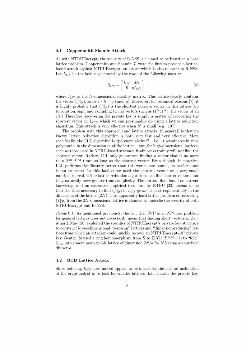
4.1 Coppersmith-Shamir Attack

As with NTRUEncrypt, the security of R-NSS is claimed to be based on a hardlattice problem. Coppersmith and Shamir [7] were the first to present a lattice-based attack against NTRUEncrypt, an attack which is also relevant to R-NSS.Let LCS be the lattice generated by the rows of the following matrix:

BCS =

[

I(N) Mh

0 qI(N)

]

, (5)

where I(N) is the N -dimensional identity matrix. This lattice clearly containsthe vector (f‖g), since f ∗ h = g (mod q). Moreover, for technical reasons [7], itis highly probable that (f‖g) is the shortest nonzero vector in this lattice (upto rotation, sign, and excluding trivial vectors such as (1N , 1N ), the vector of all1’s.) Therefore, recovering the private key is simply a matter of recovering theshortest vector in LCS , which we can presumably do using a lattice reductionalgorithm. This attack is very effective when N is small (e.g., 107).

The problem with this approach (and lattice attacks, in general) is that noknown lattice reduction algorithm is both very fast and very effective. Morespecifically, the LLL algorithm is “polynomial-time” – i.e., it terminates in timepolynomial in the dimension m of the lattice – but, for high-dimensional lattices,such as those used in NTRU-based schemes, it almost certainly will not find theshortest vector. Rather, LLL only guarantees finding a vector that is no morethan 2(m−1)/2 times as long as the shortest vector. Even though, in practice,LLL performs significantly better than this worst case bound, its performanceis not sufficient for this lattice; we need the shortest vector or a very smallmultiple thereof. Other lattice reduction algorithms can find shorter vectors, butthey naturally have greater time-complexity. The bottom line, based on currentknowledge and on extensive empirical tests run by NTRU [23], seems to bethat the time necessary to find (f‖g) in LCS grows at least exponentially in thedimension of the lattice (2N). This apparently hard lattice problem of recovering(f‖g) from the 2N -dimensional lattice is claimed to underlie the security of bothNTRUEncrypt and R-NSS.

Remark 1. As mentioned previously, the fact that SVP is an NP-hard problemfor general lattices does not necessarily mean that finding short vectors in LCS

is hard. May [20] exploited the specifics of NTRUEncrypt’s private key structureto construct lower-dimensional “zero-run” lattices and “dimension-reducing” lat-tices from which an attacker could quickly recover an NTRUEncrypt-107 privatekey. Gentry [8] used a ring homomorphism from R to Z[X]/(XN/d−1) to “fold”LCS into a more manageable lattice of dimension 2N/d for N having a nontrivialdivisor d.

4.2 GCD Lattice Attack

Since reducing LCS does indeed appear to be infeasible, the natural inclinationof the cryptanalyst is to look for smaller lattices that contain the private key.

8

The authors of R-NSS mention one such lattice in [16]. They observe that ifan attacker is able to recover the values of several f ∗ w’s in R – “unreduced”modulo q – then f will likely be the shortest vector in the N -dimensional latticeformed by the rows of the several Mf∗w’s.

Recall from section 2.2 that, for any polynomial a, there is an equivalencebetween the ideal (a) of a-multiples and the lattice generated by Ma. Similarly,the lattice spanned by the rows of Mf∗w1

and Mf∗w2corresponds to the ideal

I = (f ∗ w1, f ∗ w2). Every polynomial in I is a multiple of f . Moreover, if (w1)and (w2) are relatively prime – i.e., there exist a, b ∈ R with a ∗w1 + b ∗w2 = 1– then f ∈ I, and we may say that GCD(f ∗ w1, f ∗ w2) = (f). This “latticeattack” is, in fact, the standard ideal-GCD algorithm, and is among the latticeideal operations discussed in [2].

Given how the wi are produced in R-NSS, (f) often is indeed the GCD oftwo unreduced signatures, and it is even more likely to be the GCD of severalunreduced signatures. Therefore, given a few unreduced signatures, we can con-struct an N -dimensional lattice whose shortest vector is likely f . The authorsof R-NSS note that, although reducing this N -dimensional lattice is still nota trivial problem for R-NSS parameters, it is much easier than reducing the2N -dimensional LCS , given the exponential relationship between dimension andrunning time. R-NSS uses “masking” techniques to prevent recovery of f ∗ w’sin R to avoid this lattice attack. (In section 5 we show that recovering f ∗w’s isnonetheless quite easy.)

4.3 Averaging Attack

The so-called “averaging attack” was first considered by Kaliski during collab-oration with Hoffstein in the context of an early precursor to NSS (see patent[12]). In this work, it was observed that in the ring R, the value f ∗ f could beobtained by an averaging attack. This attack was fatal, since in the scheme [12],f itself is a palindrome (unlike in R-NSS), thus f ∗ f = f 2. There is an efficientalgorithm for taking the square root in R (see, e.g., [13]), so f ∗ f revealed f .

In [16], the authors of R-NSS do mention this averaging attack, but alsoremark that knowledge of f ∗ f does not appear to be useful. See [16], [9], [21]for a discussion of this and other ways in which the attacker may average atranscript of signatures in such a way as to get information about the privatekey.

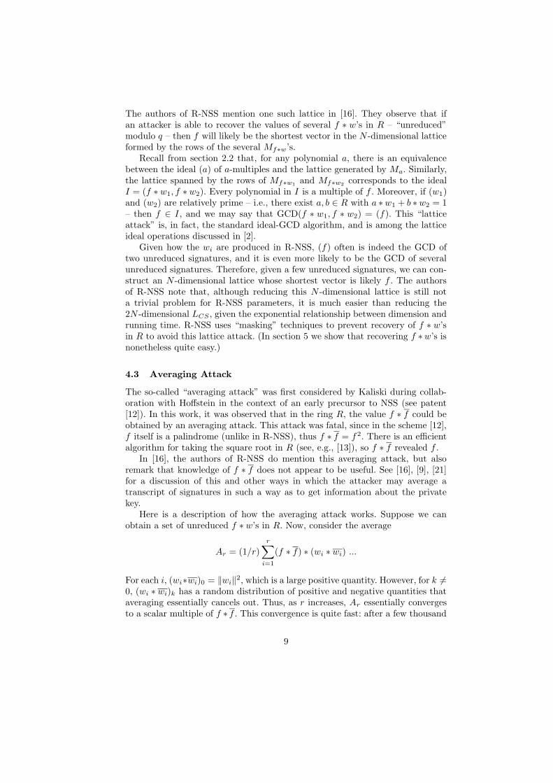
Here is a description of how the averaging attack works. Suppose we canobtain a set of unreduced f ∗ w’s in R. Now, consider the average

Ar = (1/r)r

∑

i=1

(f ∗ f) ∗ (wi ∗ wi) ...

For each i, (wi∗wi)0 = ‖wi‖2, which is a large positive quantity. However, for k 6=0, (wi ∗ wi)k has a random distribution of positive and negative quantities thataveraging essentially cancels out. Thus, as r increases, Ar essentially convergesto a scalar multiple of f ∗ f . This convergence is quite fast: after a few thousand

9

signatures a close estimate of f ∗ f can be computed, meaning that we obtainan estimate z such that for most coefficients, |zi − (f ∗ f)i| ≤ 2. Even if reducedsignatures are used, with some corrections, there is still a convergence to f ∗f , albeit about 10 times as slow. Clearly, the more signatures, the better theestimate. In section 6, we explain how this averaging attack may be combinedwith a lattice attack to recover f ∗ f quickly and completely.

5 Lifting the Signatures

In this section, we present our first (and arguably the most important) attackwith which we obtain R-multiples of the private key f . More specifically, weassume that, as passive adversaries, we are given a transcript of legitimate sig-natures {(m1, s1), . . . , (mr, sr)}. Using this transcript and the signer’s publickey, we directly compute the following elements in Rq:

{f ∗ w1 mod q, . . . , f ∗ wr mod q} and {g ∗ w1 mod q, . . . , g ∗ wr mod q} ,

where the wi are computed according to the signing process above. We will thenlift these signatures to the ring R, obtaining a list of multiples of f and g:

{f ∗ w1, . . . , f ∗ wr} and {g ∗ w1, . . . , g ∗ wr} ,

which are “unreduced” modulo q. This is a devastating attack against R-NSS,because undoing the q modular reduction of the signatures allows us to use theN -dimensional GCD lattice attack, described in section 4.2, rather than the 2N -dimensional Coppersmith-Shamir attack, reducing the key recovery time by afactor exponential in N . It also permits the other, more efficient attacks discussedlater in this paper.

5.1 The Principle

¿From the signing procedure in the ring Rq, we get the following equations foreach i:

f ∗ wi ≡ si mod q and g ∗ wi ≡ ti mod q , (6)

f ∗ wi ≡ g ∗ wi ≡ mi + ei mod p . (7)

If we knew ei, we would be able to compute f ∗ wi and g ∗ wi modulo pq viathe Chinese Remainder Theorem. We could then recover f ∗ wi and g ∗ wi overR without too much difficulty, since almost all of the coefficients of f ∗ wi andg ∗ wi will lie in the interval (−pq/2, pq/2].2

The use of ei in the signing process makes lifting the signatures much lessstraightforward. Since ei will have about 20 nonzero coefficients for the sug-gested parameters of R-NSS, we cannot simply guess ei from among

(

25120

)

220

2 See [7] for an analysis of the coefficient distributions of convolution products. Thekey points here are that L2 norms ‖f‖, ‖g‖ and ‖wi‖ are small, ‖f ∗wi‖ ≈ ‖f‖‖wi‖and the coefficients of f ∗ wi have a roughly normal distribution.

10

possibilities. Later, we will mention how specific properties of the signing pro-cess make some possibilities much more probable than others, but even withthese refinements the guessing approach remains infeasible.

Instead, we will use an iterative approach that, at each step, attempts to im-prove upon previous approximations. Let Si denote our approximation of f ∗wi,and Ti our approximation of g ∗wi. We initialize Si and Ti to be the polynomialsin Rpq that satisfy

Si ≡ si mod q and Ti ≡ ti mod q , (8)

Si ≡ Ti ≡ mi mod p . (9)

Our approximations will have two different types of errors. First, the kth coeffi-cients of Si and Ti will be wrong if the kth coefficient of ei is nonzero. Second, acoefficient of Si (resp. Ti) may be correct modulo pq but incorrect in R if the cor-responding coefficient of f∗wi (resp. g∗wi) lies outside the interval (−pq/2, pq/2].On average, about 25 (out of 251) coefficients of our initial approximations willbe incorrect.

In refining our approximations, we begin with the following observation: Forany (i, j),

(f ∗ wi) ∗ (g ∗ wj) − (f ∗ wj) ∗ (g ∗ wi) = 0 . (10)

Based on this observation, we would expect Si ∗ Tj − Sj ∗ Ti to tend towards 0as our approximations improve. In fact, this is the case. We can use the normsnij = ‖Si∗Tj−Sj ∗Ti‖ to decide what adjustments we should make, and to knowwhen our approximations are finally correct. The rest of the lifting procedureis simply an elaboration of this basic idea, and one can imagine a variety ofdifferent methods through which an attacker could use these norms to create aneffective lifting procedure. In our particular implementation against R-NSS, weused the norms nij , together with some R-NSS-specific heuristics, to create avery fast lifting procedure that worked almost all the time with a transcript ofonly four signatures.

5.2 Our Implementation of the Lifting Procedure

For each approximation pair (Si, Ti), we computed a “norm product” with theother approximation pairs according to the formula Pi =

∏

j 6=i nij . Preferringapproximation pairs with higher norm products, we then picked a random pair(Si, Ti) to be corrected. For each coefficient position, we temporarily added orsubtracted certain multiples of q to Si and Ti (since the approximations arealready correct modulo q), and recomputed Pi. With a little bookkeeping, thisstep can be made extremely fast. We preserved the adjustment that reducedPi by the greatest amount. Finally, we terminated this process when the normproduct of some approximation pair reached zero, at which point we would havetwo correct approximation pairs.

We also used some heuristics based on specific properties of the signing pro-cess to improve the performance. We make the observation that the coefficients

11

of (f ∗ wi, g ∗ wi) come from a probability distribution, which by the equationsabove, is correlated to that of ei and the initial value of (Si, Ti). Specifically, theway in which ei is computed makes it highly probable that if the kth coefficientof ei is nonzero, then the kth coefficients of the initial approximation pair (Si, Ti)will both be fairly small – e.g., in the range [−100, 100]. On the other hand, ifa coefficient of the initial Si or Ti is off by a multiple of pq, then it is highlyprobable that this coefficient is fairly large – e.g., outside the range [−100, 100].Consequently, if corresponding coefficients of the initial Si and Ti are both in[−100, 100], we might only consider adjusting these coefficients by ±q; and ifeither of these coefficients is outside [−100, 100], we might only try adjusting by−pq or pq (depending on whether the original coefficient was initially positive ornegative, respectively). In our implementation, we used precisely this heuristicin the early stages of our lifting procedure. We would then “shift gears,” consid-ering adjustments by other multiples of q so that we could catch low-probabilityerrors as well.

We note that not every adjustment made during the lifting procedure is actu-ally a correction. Often, this procedure will make a previously correct coefficientincorrect, and then switch it back later on. In other words, it behaves somewhatlike a “random walk”. This fact, together with the heuristic nature of the over-all algorithm, admittedly makes the lifting procedure difficult to analyze. Forthe specified parameters of R-NSS, however, it works quickly and reliably. For atranscript of four signatures, it is able to lift two signatures 90% of the time inan average of about 25 seconds (on a desktop computer). In the remaining 10%,the number of errors never converges to zero. For three signatures, it still works70% of the time, typically finishing in about 15 seconds.

6 Obtaining f ∗ f

An important ingredient of the final algorithm is the product of f with its rever-sal, f . In order to recover f ∗ f in the context of R-NSS, we used a combinationof the averaging attack mentioned in section 4.3 and a lattice attack on f ∗ fnoticed by the authors and Jonsson, Nguyen and Stern.

The lattice attack is a derivative of the Coppersmith-Shamir attack describedin section 4.2. Since sending a polynomial to its reversal is an automorphism,(f ∗ f) ∗ (h ∗ h) ≡ (g ∗ g) (mod q). This means that the vector (f ∗ f‖g ∗ g) iscontained in the lattice Lnorm generated by

Bnorm =

[

I(N) Mh∗h

0 qI(N)

]

. (11)

This lattice has dimension 2N , but it has an (N + 1)-dimensional sublattice ofpalindromes, which contains (f ∗ f‖g ∗ g). Conceivably, recovering (f ∗ f‖g ∗ g)from this sublattice could give us useful information about f and g. However,

12

this attack fails for typical NTRU or NSS parameters, since (f ∗ f‖g ∗ g) isnormally not the shortest vector.3

For R-NSS, we combine ideas from the above attack with the GCD attack in4.2 and the averaging technique in 4.3. First, we use our unreduced signatures toform the ideal (f∗f) from a few unreduced signature products s∗s = f∗f∗wi∗wi,exactly as described in Section 4.2. Then, we take the subring of (f ∗f) consistingof palindromes, which forms a lattice of dimension (N +1)/2. In fact, this latticeis generated by f ∗ f , and (N − 1)/2 vectors (Xk + XN−k) ∗ f ∗ f . For the samereason as above, f ∗ f might not be the shortest vector in the lattice. However,we may use the averaging attack to obtain a good estimate t of f ∗ f , modifythe lattice to include t, and then use lattice reduction to obtain the (shortest)vector t − f ∗ f .4 In practice, this attack is amazingly effective for two reasons:the lattice problem is only (N + 1)/2 dimensional, and ‖t− f ∗ f‖ will be muchless than ‖f ∗ f‖ for even a very poor estimate of t. We found that we neededonly 10 signatures to obtain a sufficiently accurate estimate t of f ∗ f (eventhough only a handful of coefficients in t were actually correct). With these 10signatures, we consistently recovered f ∗ f in less than 10 seconds.

7 Orthogonal Congruence Attack

In this section, we describe a polynomial-time algorithm for recovering the pri-vate key f from f ∗ f and one other multiple of f , such as f ∗ w, when w isrelatively prime to f . In other words, this algorithm requires f ∗ f and a basisBf of the ideal (f). 5 This algorithm is quite surprising, and uses novel ideascombining orthogonal lattices with number theoretic congruence arising fromthe cyclotomic field Q(ζN ).

The complete algorithm is rather complex, but here is a brief (and not entirelyaccurate) sketch: We begin by choosing a large prime number P ≡ 1 (mod N).(For now, we defer discussing how large P must be.) Then, using f ∗ f and ourbasis for (f), we use a series of lattice reductions to obtain fP−1 ∗ a for somepolynomial a, and a guarantee that ‖a‖ < P/2. Using the congruence fP−1 ≡ 1(mod P ), we will be able to compute a (mod P ) and hence a exactly, from whichwe will be able to compute fP−1 exactly. We will then use this power of f torecover f .

3 By the “Gaussian heuristic,” the expected length of the shortest vector in a lat-tice of determinant d and dimension n is d1/n

√

n/(2πe). For Lnorm, this length is√

qN/(πe). On the other hand, since ‖f‖ >√

N in NSS and ‖f ∗ f‖ ≥ ‖f‖2 (thelatter inequality following from (f ∗ f)0 = ‖f‖2), the norm of f ∗ f is greater thanN and hence greater than the Gaussian heuristic, since N is typically chosen to begreater than q.

4 One could also use Babai’s algorithm to solve the closest vector problem (CVP).5 Yet another characterization of the algorithm is that it recovers f from Bf and the

relative norm of f over the index 2 subfield of Q(ζN ).

13

We describe this algorithm and the theory behind it in more detail below.Our first task will be to find a tool that ensures that when LLL gives us fP−1∗a,there is a definite bound on ‖a‖.

7.1 Orthogonal Lattices

Certain lattices possess a basis of N equal length, mutually perpendicular basisvectors. We denote such lattices orthogonal lattices. Two lattices are called ho-mothetic if up to a constant stretching factor, λ, there is a distance preservingmap from one lattice to the other. That is, all orthogonal lattices are homotheticto the trivial lattice ZN . Similarly, we define f to be an orthogonal polynomialif the circulant matrix Mf is the orthogonal basis of an orthogonal lattice. Weare interested in orthogonal lattices because they possess a multiplicative normproperty.

We note that for randomly chosen polynomials a and f , the norm is quasi-multiplicative, ‖f ∗a‖ ≈ ‖f‖ · ‖a‖. However, if one of the polynomial factors, sayf , is orthogonal, then equality will hold

‖f ∗ a‖ = ‖f‖ · ‖a‖ . (12)

For general polynomials f , applying LLL to (f) is guaranteed to find a multipleof f , say f ∗ a, such that the norm ‖f ∗ a‖ is less than a specific factor times thenorm of the shortest vector in the lattice. In the case where f is orthogonal, wecan additionally bound ‖a‖ by this factor, since ‖f ∗ a‖ = ‖f‖ · ‖a‖. In the caseof LLL, this means that we can be certain that ‖a‖ < 2(N−1)/2.

7.2 Using f ∗ f to Construct an Implicit Orthogonal Lattice

What do we do when f is not an orthogonal polynomial, but our objective isto find f ∗ a with small ‖a‖ (given only f ∗ f and lattice basis Bf of (f))? Ofcourse, we may apply LLL to Bf and just hope that the output vector f ∗ a hasshort a, but this may not work even if f is only slightly nonorthogonal6. Thissection describes how we can accomplish this task by using knowledge of f ∗ fto implicitly define an orthogonal lattice.

Since Bf and Mf are both bases of (f), they are related by Bf = U · Mf

for some unimodular matrix U . Notice that each row of Bf is of the form f ∗ ui

where ui is the ith row of U . This means that the objective of finding f ∗ a withbounded ‖a‖ is equivalent to bounding the norms of the rows of U . So, in somesense, we would like to apply lattice reduction to U . How can we reduce the rowsof U when we only know Bf = U · Mf , and not U itself?

Supposing that f is a not a zero divisor in R, we can also divide by f ∗ f .Allowing denominators in our notation, we let D = M(1/(f∗f)) and compute

Bf · D · BTf = U · UT , (13)

6 The notion of nonorthogonality is made precise with concept called orthogonalitydefect.

14

which is the Gram matrix of our unknown unimodular matrix U . Although wedo not know U explicitly, U ·UT has all the information that LLL needs to knowabout U in order to reduce it – namely, the mutual dot products ui · uj of eachpair of row vectors. We can therefore apply a Gram matrix version of LLL toU · UT , which outputs the unimodular transformation matrix V , and the Grammatrix of the reduced lattice: (V · U) · (V · U)T . By the LLL bound, the normsof the rows of (the unknown) basis V ·U will be bounded by 2(N−1)/2. Now, wecan compute a new basis of (f) – namely, (V ·U) ·Mf = V ·Bf – and be certainthat each row of this basis equals f ∗ai for ‖ai‖ < 2(N−1)/2. Effectively, we havereduced the orthogonal lattice defined by U , without even knowing an explicitbasis for it.

7.3 Galois Congruence

In addition to the orthogonal lattices technique, we use some interesting congru-ences on the ring R. The first congruence states that for any prime P such thatP ≡ 1 (mod N),

fP = f (mod P ) . (14)

This implies that for any f which is not a zero divisor7 in RP = ZP [X]/(XN −1)that

fP−1 = 1 (mod P ) . (15)

We may generalize these equations to arbitrary primes P by using a GaloisConjugation function (written as a superscript) σ(r) : R → R, defined by

fσ(r)(x) = f(xr). (16)

For any r not divisible by N , σ(r) defines an automorphism on R. There are N−1such automorphisms, since two values of r which differ by a factor of N definethe same automorphism. We call σ(r) the rth Galois conjugation mapping, andhave the congruence

fP = fσ(P ) (mod P ) . (17)

For elementary proofs of equations 15 and 17 and their relationship with the theGalois theory of Q(ζ), we refer the reader to the Appendix E; for the relationshipwith the the Galois theory of Q(ζ), see Appendix D.

As mentioned above, our motivation for considering such congruences is thatgiven a multiple of fP−1, say fP−1 ∗ a, we may use the congruence fP−1 = 1(mod P ) to conclude that

fP−1 ∗ a = a (mod P ) . (18)

Now, if a is so small that all of its coefficients lie in the interval (−P/2, P/2],then the representatives for fP−1 ∗ a (mod p) in this interval reveal a exactly.Assuming that a is not a zero divisor in R, dividing the product by a then

7 See Appendix E for a discussion of the zero divisor issue in RP .

15

yields the exact value of fP−1. With this observation, we are in a position touse orthogonal lattice theory with lattice reduction to obtain small multiples ofpowers of f and thus exact powers of f .

However, there is a technical difficulty arising from the fact that LLL onlyguarantees that ‖a‖ < 2(N−1)/2. To ensure that a has coefficients in (−P/2, P/2],P has to be quite large – about the same order of magnitude as 2(N−1)/2. Thismeans that fP−1 has bit-length exponential in N , which makes it impossible forus to even store the value of this polynomial. Initially, this might appear to bea fatal problem. It also indicates that the “brief sketch” given at the beginningof Section 7 could not have been entirely accurate.

Fortunately, we will not need to work with fP−1 directly; it will be sufficientfor our purposes to be able to compute fP−1 modulo some primes. As discussedfurther in section 7.4, we can make such computations using a process similarto repeated squaring. However, to recover f , we will need some power of f thatwe can work with directly (unreduced). To solve this problem, we may choosea second prime P ′ ≡ 1 (mod N) with GCD(P − 1, P ′ − 1) = 2N for which wecan compute fP ′−1 modulo some primes. Then, using the Euclidean Algorithm,we may compute f2N modulo these primes, and ultimately f 2N exactly viathe Chinese Remainder Theorem. We may work with f 2N directly, since itsbit-length is merely polynomial in N . A more elegant solution in Appendix Fcomputes f2N directly from fP−1 if GCD(P − 1, 2N − 1) = 1. In Section 7.5,we describe how to recover f from f 2N .

7.4 Ideal Power Algorithms

In practice, it might be the case that smaller P would be sufficient, allowing usto work with the ideal (fP−1) directly, but some tricks are needed to handle thevery large primes P that the LLL bound imposes on us. Suppose we had thechains of polynomials {v2

0 ∗v1, . . . , v2r−1 ∗vr} and {v0 ∗v0, . . . , vr−1 ∗vr−1}. Then,

we could make the following series of computations:

v40 ∗ v2 = (v2

0 ∗ v1)2 ∗ (v1 ∗ v1)

−2 ∗ (v21 ∗ v2) (mod P ) , (19)

v80 ∗ v3 = (v4

0 ∗ v2)2 ∗ (v2 ∗ v2)

−2 ∗ (v22 ∗ v3) (mod P ) , (20)

and so on, ending with the equation:

v2r

0 ∗ vr = (v2r−1

0 ∗ vr−1)2 ∗ (vr−1 ∗ vr−1)

−2 ∗ (v2r−1 ∗ vr) (mod P ) . (21)

In other words, we could compute v2r

0 ∗ vr (mod P ) efficiently even though theexponent 2r may be quite large. If we could use this approach to get vP−1

0 ∗ vr

(mod P ) where ‖vr‖ < P/2, then we could recover vr exactly, and then we coulduse the same chains of polynomials to compute vP−1

0 modulo other primes.In this section, we describe how to get such chains of polynomials so that

we can get modular data about fP−1 from f ∗ f and a basis Bf of (f). Themain tool that we use is the multiplication of ideals (see [2]), and we adapt thistechnique to use the orthogonal lattice theory above. The algorithm described

16

in the paragraph above is essentially a repeated squaring algorithm, so we firstreview how to multiply ideals, and in particular, obtain the ideal (f 2) from theideal (f).

Remark 2. Ideal multiplication in R: If A = (f) and B = (g) are principal idealsgenerated as Z-modules by (f ∗ a1, . . . , f ∗ an) and (g ∗ b1, . . . , g ∗ bn), then theideal product AB is generated as a Z-module by the n2 elements of the set{ai ∗ bj ∗ f ∗ g}, which defines (f ∗ g).

Note that we describe the ideals as modules – i.e., as the Z-span of a set ofpolynomials (rather than by giving generators over R). This is because our al-gorithms represent ideals as lattices – i.e., as lists of polynomials. We use idealmultiplication as follows: Given the ideal (f) in terms of the basis Bf = U ·Mf ,

we can generate (f2) from the rows bi ∗ bj = ui ∗ uj ∗ f2. Since we know f2 ∗ f2,

we can use the orthogonal lattice method described in section 7.2 to obtain areduced basis Bf2 = U ′Mf2 where the rows of U ′ have norm less than 2(N−1)/2.8

Next, we pick a row of Bf2 and name it f2 ∗ v1. We can directly compute v1 ∗ v1

and a basis for v1: U ′ · Mv1. At this point we can compute a basis for (v2

1) tobegin another iteration of this process. Thus, we have the chains of polynomialspreviously introduced, and, with a modification to multiply some of the ideals by(f), its natural generalization. (Note: v0 represents f in the following theorem.)

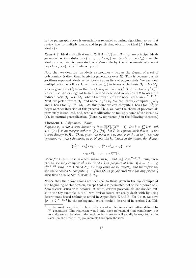
Theorem 1. Polynomial ChainsSuppose v0 is not a zero divisor in R = Z[X]/(XN − 1). Let k =

∑

ki2i with

ki ∈ {0, 1} be an integer with r = blog2(k)c. Let P be a prime such that v0 is nota zero divisor in RP . Then, given the input v0 ∗ v0 and basis B0 of (v0), we maycompute, in time polynomial in r, N and the bit-length of the input, the chains:

{vkr−1

0 ∗ v20 ∗ v1, . . . , v

k0

0 ∗ v2r−1 ∗ vr} and

{v0 ∗ v0, . . . , vr−1 ∗ vr−1},where for ∀i > 0, no vi is a zero divisor in RP , and ‖vi‖ < 2(N−1)/2. Using thesechains, we may compute vk

0 ∗ vr (mod P ) in polynomial time. If k = P − 1 ≥2(N+1)/2 with P ≡ 1 (mod N), we may compute vr exactly, and thereafter usethe above chains to compute vP−1

0 (mod Q) in polynomial time for any prime Qsuch that no vi is zero divisor in RQ.

Notice that the above chains are identical to those given in the toy example atthe beginning of this section, except that k is permitted not to be a power of 2.Zero-divisor issues arise because, at times, certain polynomials are divided out,as in the toy example, but all zero divisor issues are easily dealt with by usingdeterminant-based technique noted in Appendices E and F. For i > 0, we have‖vi‖ < 2(N−1)/2 by the orthogonal lattice method described in section 7.2. This

8 In the worst case, this involves reduction of an N -dimensional lattice defined byN2 generators. This reduction would only have polynomial time-complexity, butnormally we will be able to do much better, since we will usually be easy to find farfewer (on the order of N) polynomials that span the ideal.

17

norm bound and the polynomial running time of LLL underlie the polynomialcomplexity of the algorithm. In the Appendix F, we write this algorithm interms of pseudocode in an effort to clarify its details as well as its polynomial-time complexity. Now, we will use the algorithm embodied in Theorem 1 toobtain f2N .

Theorem 2. Computing f2N

Assume f is not a zero divisor in R = Z[X]/(XN − 1). Then, given f ∗ f andbasis Bf of (f), we may compute f2N in time polynomial in N and the bit-lengthof f .

Proof. We choose primes P and P ′, each greater than 2(N+1)/2, with GCD(P −1, P ′ − 1) = 2N and f is a zero divisor in neither RP nor RP ′ (using Dirichlet’stheorem on primes in arithmetic progression and the fact that f may be a zerodivisor in RQ for only a finite number of primes Q). By Theorem 1, we maycompute two polynomial chains that will allow us to compute fP−1 (mod ri)and fP ′−1 (mod ri) in polynomial time for any prime ri such that no vi (in eitherchain) is zero divisor in Rri

. (We simply avoid the finite number of problematicprimes.) Applying the Euclidean algorithm, we compute f 2N modulo each ri,and ultimately f2N exactly using the Chinese Remainder Theorem.

7.5 Computing f from f2N

Our final task is to compute the private key f from f 2N . We use the followingtheorem.

Theorem 3. Galois PolynomialGiven f2N and b ∈ Z∗

N , we may compute z = fσ(−b)f b in time polynomial in b,N and bit-length of f .

Proof. Let P2 > 2‖fσ(−b)f b‖ be a prime number such that P2 = 2c2N − bfor some integer c2. Then, (f2N )c2 ≡ fP2 ∗ f b ≡ fσ(−b)f b (mod P2). SinceP2 > 2‖fσ(−b)f b‖, we recover z = fσ(−b)f b exactly.

Now, in terms of recovering f , we first note that f 2N uniquely defines f onlyup to sign and rotation – i.e., up to multiplication by ±Xk, the 2Nth roots ofunity in R. The basic idea of our approach is that, given f 2N , fixing f(ζ) for one(complex) Nth root of unity ζ completely determines f(ζd) for all exponents d.Then, we may use the N − 1 values of f(ζd), together with f(1) (which we willknow up to sign), to solve for f using Gaussian elimination. If we set −b to bea primitive root modulo N , the polynomial z given in Theorem 3 will help usiteratively derive the f(ζd) from f(ζ) as follows:

f(ζ(−b)i+1

) = z(ζ(−b)i

)/f b(ζ(−b)i

) . (22)

Repeated exponentiation will not result in a loss of precision, since the valuemay be corrected at each stage. Since −b is a primitive root modulo N , theseevaluations give us N − 1 linearly independent equations in the coefficients of f ,which together with f(1), allow us to recover the private key f completely, upto sign and rotation.

18

8 Summary and Generalizations of R-NSS Cryptanalysis

For the reader’s convenience, we briefly review the main points of the attack. Thefirst two stages of the attack are fast in practice, but they are both heuristic andhave no proven time bounds. The lifting procedure lifts a transcript of signaturesfrom Rq to R, obtaining unreduced f -multiples in R. The second stage usesan averaging attack to approximate f ∗ f , and then solves the closest vectorproblem (CVP) to recover f ∗ f exactly. The algorithm of the final stage, whichwe have not fully implemented, uses output from the previous two stages torecover the private key in polynomial time. By combining lattice-based methodsand number-theoretic congruences, the algorithm of the final stage can be usedto:

1. Recover f from f ∗ f and a basis Bf of (f);2. Recover f from only Bf when f is an orthogonal polynomial; and3. Recover f/f from Bf whether f is an orthogonal polynomial or not.

We anticipate that this algorithm could be generalized to recover f given a basisof (f) and the relative norm of f over an index 2 subfield where the degree-2 extension is complex conjugation. In Section 9, we discuss another possiblegeneralization of this algorithm that may be an interesting area of research.

9 NTRUSign

NTRUSign was proposed at the rump session of Asiacrypt 2001 as a replace-ment of R-NSS [11], and, as requested by the Program Committee, we providesome preliminary security analysis. The scheme is more natural than previousNTRU-based signature schemes, particularly in terms of its sole verification cri-terion: the signer (or forger) must solve an “approximate CVP problem” in theNTRU lattice – i.e., produce a lattice point that is sufficiently close to a messagedigest point, a la Goldreich, Goldwasser and Halevi [10]. Similar to the GGHcryptosystem, the signer has private knowledge of a “good” basis of the NTRUlattice having short basis vectors, and publishes the usual “bad” NTRU latticebasis:

Bpriv =

[

Mf Mg

MF MG

]

Bpub =

[

I(N) Mh

0 qI(N)

]

.

Unlike GGH, these bases may be succinctly represented with only four polyno-mials: (f, g, F,G) for the private basis, and h for the public basis. (Recall thatMf denotes the circulant matrix corresponding to the polynomial f ; see Section2.) In terms of key generation, the signer first generates short polynomials f andg and computes the public key as h = f−1 ∗ g (mod q), as in NTRUEncrypt orR-NSS. Due to lack of space, we refer the reader to [11] for details on how thesigner generates his second pair of short polynomials (F,G), but we note thefollowing properties: 1) f ∗ G − g ∗ F = q and 2) ‖F‖ and ‖G‖ are 2 to 3 timesgreater than ‖f‖ and ‖g‖.

19

To sign, the message is hashed to create a random message digest vector(m1,m2) with m1,m2 ∈ Rq. The signer then computes:

G ∗ m1 − F ∗ m2 = A + q ∗ C , (23a)

−g ∗ m1 + f ∗ m2 = a + q ∗ c , (23b)

where A and a have coefficients in (−q/2, q/2], and sends his signature:

s ≡ f ∗ C + F ∗ c (mod q) . (24)

The verifier computes t ≡ s ∗ h (mod q) and checks that (s, t) is “close enough”to (m1,m2) – specifically,

‖s − m1‖2 + ‖t − m2‖2 ≤ Normbound . (25)

We can see why verification works when we write, say, s in terms of Equations23a and 23b:

s ≡ m1 − (A ∗ f + a ∗ F )/q (mod q) , (26)

where ‖A ∗ f + a ∗ F‖ will be reasonably short since f and F are short.In the absence of a transcript, the forgery problem is provably as difficult as

the approximate CVP problem in the NTRU lattice. However, it is clear thatNTRUSign signatures leak some information about the private key. The map-ping involution Z[X]/(q,XN − 1) sending m 7→ s is not a permutation, andthe associated identification protocol is not zero knowledge (even statisticallyor computationally). Below, we describe concrete transcript attacks using ideasfrom our cryptanalysis of R-NSS. We have had fruitful discussions with NTRUregarding these attacks, and they have begun running preliminary tests to de-termine their efficacy. Based on these tests, some of these attacks appear torequire a very long transcript that may make them infeasible in practice. Thisis a subject of further research. In any case, these attacks show that NTRUSigncannot have any formal security property, since it is not secure against passiveadversaries.

9.1 Second Order Attack

Using Equation 26, we may obtain polynomials of the form (A ∗ f + a ∗ F )(similarly, (A ∗ g + a ∗ G)). Consider the following average:

Avgff (r) = (1/r)

r∑

i=1

(ai ∗ F + Ai ∗ f) ∗ (ai ∗ F + Ai ∗ f) (27)

= (1/r)r

∑

i=1

(ai ∗ ai) ∗ (F ∗ F ) + (Ai ∗ Ai) ∗ (f ∗ f) + other terms .

(28)

The “other terms” will converge to 0, since A and a are uniformly distributed atrandom modulo q and, though dependent, have small statistical correlation. (See

20

Remark 3 below.) The explicit portion of the average will converge essentiallyto a scalar multiple of f ∗ f +F ∗F , for the same reasons as discussed in Section4.3. Thus,

lim Avgff (r) = γ(f ∗ f + F ∗ F ) . (29)

Because the signatures in a transcript are random variables, the limit convergesas 1/

√r where r is the length of a transcript. We may use this averaging to

obtain a sufficiently close approximation of f ∗ f + F ∗ F to obtain the exactvalue by solving the CVP in the (N + 1)-dimensional lattice given in Equation11 using lattice reduction. Thus, we recover a polynomial that is quadratic inthe private key, and we can obtain f ∗ g + F ∗ G and g ∗ g + G ∗ G in a similarfashion.

Remark 3. One may artificially construct situations where (1/r)∑r

i=1 ai ∗ Ai

does not converge to 0. For example, if we let f = F , then Ai ∗ f + ai ∗ F ≡ 0(mod q) basically implies Ai = −ai and hence ai ∗ Ai = −ai ∗ ai, the average ofwhich does not converge to 0. Conceivably, NTRUSign could be modified so asto constrain f−1 ∗ F (mod q), but this would likely allow alternative attacks.

It is worth noting that these second order polynomials give us the Grammatrix BT

priv · Bpriv:

BTpriv · Bpriv =

[

Mf MF

Mg MG

] [

Mf Mg

MF MG

]

=

[

Mf∗f+F∗F Mg∗f+G∗F

Mf∗g+F∗G Mg∗g+G∗G

]

.

This Gram matrix gives us the “shape” of the parallelepiped defined by BTpriv,

but the “orientation” of this parallelepiped is unclear. An interesting (and open)question is: Can an attacker recover Bpriv from BT

priv · Bpriv and Bpub = U ·Bpriv, where U is a unimodular matrix? We answered a similar question in theaffirmative in Section 7; we showed that an attacker, in polynomial time, canrecover Mf from MT

f · Mf and U · Mf , where U is a unimodular matrix. Wehave not found a way to extend the orthogonal congruence attack to solve theNTRUSign Gram matrix problem, however, where the bi-circulant (rather thanpurely circulant) nature of the matrices in question (such as Bpriv) destroys thecommutativity that our orthogonal congruence attack appears to require, butthis does not imply that the NTRUSign Gram matrix problem is necessarilyhard. We note that it would more than suffice to find an algorithm that factorsU ·UT for unimodular U . (This factorization is unique up to a signed permutationmatrix.) Further research in this area would be interesting, if only because it isrelevant to NTRUSign’s security.

9.2 Second Order Subtranscript Attack

It is clear that the second order polynomials recovered above contain informationnot contained in the public key, but using this information to create an effectiveattack is not so straightforward. Our approach has been to use the second orderpolynomials to recover, say, f ∗ f , so that we may then apply the orthogonal

21

congruence attack to recover f . One way to get f ∗ f is to use the followingsubtranscript attack.

First, we notice that since ‖F‖ > ‖f‖, the norm ‖A ∗ f + a ∗ F‖ is dictatedmore by ‖a‖ than by ‖A‖. More relevantly, for our purposes, an A∗f +a∗F thatis longer than normal will usually have ‖a‖ > ‖A‖. This suggests a subtranscriptattack, including in Equation 27 only those polynomials Ai ∗f +ai ∗F for which‖Ai ∗ f + ai ∗ F‖ is greater than some bound.9 Then, we have:

Subtranscript: lim Avgff (r) = γ1(f ∗ f) + γ2(F ∗ F ) , (30)

for γ1 < γ2. Since this linear combination of f ∗ f and F ∗ F is distinct fromthat in Equation 29, we may compute f ∗ f and F ∗ F . The convergence of thissubtranscript averaging will be affected by the proportional size of the subtran-script, but more importantly, by the fact that γ1 may be only a few percentagepoints greater than γ2 (in our preliminary experiments using the longest 50% ofthe Ai∗f+ai∗F ’s). Further experiments are necessary to determine the effective-ness of this attack. Another consideration is that in [11], a possible modificationof NTRUSign was proposed in which one chooses the transpose of Bpriv to bethe private key. The basis vectors are then (f, F ) and (g,G) with ‖f‖ ≈ ‖g‖and ‖F‖ ≈ ‖G‖. Choosing the private basis in this way appears to defeat thissubtranscript attack.

9.3 Fourth Order Attack

An alternative way to get f∗f is to use the following fourth order attack. Viewingthe average in Equation 27, one may consider the corresponding variance andconclude, under the assumption of the statistical independence of a and A, that:

limr→∞

(1/r)

r∑

i=1

(s ∗ srev)2 − (1/r)β( limr→∞

r∑

i=1

(s ∗ srev))2 = γf ∗ f ∗ F ∗ F . (31)

The adjustment value of β depends on the scheme parameters n and q, and sothe above value may not be exactly the variance. The factor γ also depends onthe scheme parameters, and is a constant that slows convergence by a factor1γ2 . This limit does converge more slowly than the second order averaging, but,as above, we may use a close approximation in conjunction with the lattice ofEquation 11 to obtain the exact value. Preliminary tests show that it may not bepractical to obtain an error lower than the Gaussian estimate with a reasonablenumber of signatures. Assuming we do obtain the value f ∗ f ∗ F ∗ F , we mayuse it in combination with (f ∗ f + F ∗ F )2 to obtain (f ∗ f − F ∗ F )2, andthen f ∗ f − F ∗ F (using, perhaps, the algorithm given in Section 7.5). Then,f ∗ f + F ∗ F and f ∗ f − F ∗ F give us f ∗ f and F ∗ F .

9 This selection criterion might be refined, as by also considering the norm of A ∗F −a ∗ f , which may be computed using the above second order polynomials.

22

9.4 Preliminary Conclusion

The approach of these initial attacks was to reduce the breaking problem tothe orthogonal congruence attack using the results of various averagings. Weshowed how this could be done, but the practical feasibility of these attacks hasyet to be determined. In our experiments, we have found that the second orderattack is feasible; for example, by averaging 20000 signatures, an attacker mayobtain an approximation whose squared error is about 88, about 1/20 of thesquared Gaussian heuristic of the (N + 1)-dimensional CVP lattice that wouldbe used to correct this approximation. Although we have not tested this CVPlattice, we believe its reduction would be feasible. Alternatively, more signaturescould first be used to obtain a better approximation. We have also shown howthe security of NTRUSign rests on the hardness of several new hard problems.These attacks will continue to be analyzed by the authors, NTRU corporation,and the cryptographic community.

10 Acknowledgments

The authors would like to thank Burt Kaliski, Alice Silverberg and Yiqun LisaYin for helpful discussions, Jakob Jonsson, Phong Nguyen, and Jacques Sternfor discussions and collaboration on the precursor of this article, and JeffreyHoffstein, Nick Howgrave-Graham, Jill Pipher, Joseph Silverman and WilliamWhyte, who have given us valuable feedback on our cryptanalysis, particularlyon our preliminary cryptanalysis of NTRUSign.

References

1. M. Ajtai, The shortest vector problem in L2 is NP-hard for randomized reductions,in Proc. 30th ACM Symposium on Theory of Computing, 1998, 10–19.

2. H. Cohen, A Course in Computational Algebraic Number Theory, Graduate Textsin Mathematics, 138. Springer, 1993.

3. H. Cohen, Advanced Topics in Computational Number Theory, Graduate Texts inMathematics 138 ,1993.

4. Consortium for Efficient Embedded Security. Efficient Embedded Security Stan-dard (EESS) # 1: Draft 1.0. Previously on http://www.ceesstandards.org.

5. Consortium for Efficient Embedded Security. Efficient Embedded Security Stan-dard (EESS) # 1: Draft 2.0. Previously on http://www.ceesstandards.org.

6. Consortium for Efficient Embedded Security. Efficient Embedded Security Stan-dard (EESS) # 1: Draft 3.0. Available from http://www.ceesstandards.org.

7. D. Coppersmith and A. Shamir, Lattice Attacks on NTRU, in Proc. of Eurocrypt’97, LNCS 1233, pages 52–61. Springer-Verlag, 1997.

8. C. Gentry, Key Recovery and Message Attacks on NTRU-Composite, in Proc. ofEurocrypt ’01, LNCS 2045, pages 182–194. Springer-Verlag, 2001.

9. C. Gentry, J. Jonsson, J. Stern, M. Szydlo, Cryptanalysis of the NTRU signaturescheme, in Proc. of Asiacrypt ’01, LNCS 2248, pages 1–20. Springer-Verlag, 2001.

23

10. O. Goldreich, S. Goldwasser, S. Halevi, Public-key Cryptography from Lattice Re-duction Problems, in Proc. of Crypto ’97, LNCS 1294, pages 112–131. Springer-Verlag, 1997.

11. J. Hoffstein, N. Howgrave-Graham, J. Pipher, J.H. Silverman, W. Whyte,NTRUSign: Digital Signatures Using the NTRU Lattice, December, 2001. Availablefrom http://www.ntru.com.

12. J. Hoffstein, B.S. Kaliski, D. Lieman, M.J.B. Robshaw, Y.L. Yin, Secure user iden-tification based on constrained polynomials, US Patent 6,076,163, June 13, 2000.

13. J. Hoffstein, D. Lieman, J.H. Silverman, Polynomial Rings and Efficient PublicKey Authentication, in Proc. International Workshop on Cryptographic Techniquesand E-Commerce (CrypTEC ’99), Hong Kong, (M. Blum and C.H. Lee, eds.), CityUniversity of Hong Kong Press.

14. J. Hoffstein, J. Pipher, J.H. Silverman, Enhanced Encoding and Verification Meth-ods for the NTRU Signature Scheme, NTRU Technical Note #017, May 2001.Available from http://www.ntru.com.

15. J. Hoffstein, J. Pipher, J.H. Silverman. Enhanced encoding and verification meth-ods for the NTRU signature scheme (ver. 2), May 30, 2001. Available fromhttp://www.ntru.com.

16. J. Hoffstein, J. Pipher, J.H. Silverman, NSS: The NTRU Signature Scheme,preprint, November 2000. Available from http://www.ntru.com.

17. J. Hoffstein, J. Pipher, J.H. Silverman, NSS: The NTRU Signature Scheme, inProc. of Eurocrypt ’01, LNCS 2045, pages 211–228. Springer-Verlag, 2001.

18. J. Hoffstein, J. Pipher, J.H. Silverman, NSS: The NTRU Signature Scheme: Theoryand Practice, preprint, 2001. Available from http://www.ntru.com.

19. A.K. Lenstra, H.W. Lenstra Jr., L. Lovasz, Factoring Polynomials with RationalCoefficients, Mathematische Ann. 261 (1982), 513–534.

20. A. May, Cryptanalysis of NTRU-107, preprint, 1999. Available fromhttp://www.informatik.uni- frankfurt.de/~alex/crypto.html.

21. I. Mironov, A Note on Cryptanalysis of the Preliminary Version of the NTRUSignature Scheme, IACR preprint server, http://eprint.iacr.org/2001/005.

22. P. Nguyen and J. Stern, Lattice Reduction in Cryptology: An Update, in Proc.of Algorithm Number Theory (ANTS IV), LNCS 1838, pages 85–112. Springer-Verlag, 2000.

23. J.H. Silverman, Estimated Breaking Times for NTRU Lattices, NTRU TechnicalNote #012, March 1999. Available from http://www.ntru.com.

24. J.H. Silverman, Invertibility in Truncated Polynomial Rings., NTRU TechnicalNote #009, October 1998. Available from http://www.ntru.com.

25. L. Washington, Introduction to Cyclotomic Fields, Graduate Texts in Mathematics83, 1982.

A Original NSS and R-NSS: The Details

This section is included for completeness, so that this paper has a completespecification of R-NSS, and so the reader can compare the original NSS to R-NSS, and see why R-NSS is not susceptible to previous attacks.

A.1 Original NSS

Like R-NSS, NSS uses the parameters N , q, p, df , dg and dm, and polynomialsf ,g and h, which play roughly the same role as in section 3.

24

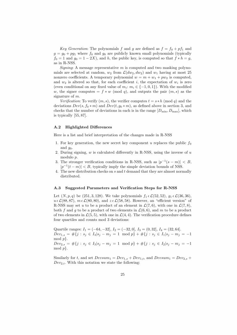
Key Generation: The polynomials f and g are defined as f = f0 + pf1 andg = g0 + pg1 where f0 and g0 are publicly known small polynomials (typicallyf0 = 1 and g0 = 1 − 2X), and h, the public key, is computed so that f ∗ h = g,as in R-NSS.

Signing: A message representative m is computed and two masking polyno-mials are selected at random, w2 from L(dw2, dw2) and w1 having at most 25nonzero coefficients. A temporary polynomial w = m + w1 + pw2 is computed,and w2 is altered so that, for each coefficient i, the expectation of wi is zero(even conditional on any fixed value of mi: mi ∈ {−1, 0, 1}). With the modifiedw, the signer computes = f ∗ w (mod q), and outputs the pair (m, s) as thesignature of m.

Verification: To verify (m, s), the verifier computes t = s∗h (mod q) and thedeviations Dev(s, f0 ∗ m) and Dev(t, g0 ∗m), as defined above in section 3, andchecks that the number of deviations in each is in the range [Dmin, Dmax], whichis typically [55, 87].

A.2 Highlighted Differences

Here is a list and brief interpretation of the changes made in R-NSS

1. For key generation, the new secret key component u replaces the public f0

and g0.2. During signing, w is calculated differently in R-NSS, using the inverse of u

modulo p.3. The stronger verification conditions in R-NSS, such as |p−1(s − m)| < B,

|p−1(t − m)| < B, typically imply the simple deviation bounds of NSS.4. The new distribution checks on s and t demand that they are almost normally

distributed.

A.3 Suggested Parameters and Verification Steps for R-NSS

Let (N, p, q) be (251, 3, 128). We take polynomials f1 εL(52, 52), g1 εL(36, 36),u εL(88, 87), mεL(80, 80), and z εL(58, 58). However, an “efficient version” ofR-NSS may set u to be a product of an element in L(7, 6), with one in L(7, 8),both f and g to be a product of two elements in L(6, 6), and m to be a productof two elements in L(5, 5), with one in L(4, 4). The verification procedure definesfour quartiles and counts mod 3 deviations:

Quartile ranges: I1 = (−64,−32], I2 = (−32, 0], I3 = (0, 32], I4 = (32, 64].Dev1,s = #{j : sj ∈ I4|sj − mj = 1 mod p} + #{j : sj ∈ I1|sj − mj = −1mod p}.Dev2,s = #{j : sj ∈ I3|sj − mj = 1 mod p} + #{j : sj ∈ I2|sj − mj = −1mod p}.

Similarly for t, and set Devsum1 = Dev1,s + Dev1,t, and Devsum1 = Dev2,s +Dev2,t. With this notation we state the following:

25

Condensed Verification Criteria

1. Require Devsum1 ≤ 10.2. Require Devsum2 ≤ 18.3. Require |(s′, t′)| < 485.4. Require |s′| < 360.5. Require |t′| < 360.6. Require between 95 and 153 coefficients of s and t to be in quartile 1.7. Require between 50 and 100 coefficients of s and t to be in quartile 2.8. Require between 7 and 42 coefficients of s and t to be in quartile 3.9. Require between 0 and 14 coefficients of s and t to be in quartile 4.

B Statistical and Forgery Attacks

Here, we briefly summarize some attacks on the original version of NSS, andhighlight how improvements in R-NSS defeat them. Admittedly, these attacks,by Gentry, Jonsson, Stern, and Szydlo [9], exploited specific weak features of NSSrather than its core, allowing NSS to be, in effect, “patched.” Refer to AppendixA for details on the previous version of NSS, and its differences from R-NSS.

The Forgery Attack provided a direct method of finding false signaturesthat satisfied the chief verification criterion, namely: Dev(s, f0 ∗ m) < 87, andDev(t, g0 ∗ m) < 87. The task was to find a pair of related polynomials (s, t)that simultaneously satisfy the deviation requirements, as well as the congruencet = s∗h (mod q). Since s and t have 2N coefficients altogether, and the equationt = s∗h (mod q) imposes N linear constraints, there remain N degrees of freedomwith which to choose the coefficients of s and t. So setting si ≡ (f0 ∗m)i mod pand tj ≡ (g0 ∗ m)j mod p for any bN/2c coefficients of s and dN/2e coefficientsof t (i.e., about half of each), the remaining halves of s and t are determined byg = h ∗ f , essentially left to chance. But the chosen half of s (resp. t) has nodeviations, and the remaining half will probabilistically deviate in about 2

3 ofthe positions, overall about 1

3 of the coefficients of s (resp. t) will deviate. Since13N ≈ 84 ≤ Dmax = 87, this technique will generate a valid forgery after only afew iterations. See [9] for some improvements using lattice reduction to improvethe chances, and “quality” of the signature.

The Transcript Attack recovered the private key from a long transcript(mi, si) of signatures using correlations between these signatures and the privatekey. For a very early version of NSS, the masking polynomials w1, and w2, werechosen at random. Taking some mi’s so that the average mi was about 1, thenthe average si would be about f , the private key. About a thousand signatureswere needed. Now, conceptually, we can think of that attack as a blatant exampleof how the coefficients fk were jointly statistically dependent on the si, and mj .Choosing w2 so that the average above was always 0 fixed this particular flaw,but the coefficients of s still basically depended on the private key f , the messagem and the polynomials w1 and w2 (which are not completely independent of m).

26

So, the same distribution concept holds: the coefficients of f depend on s in away which is not independent of m. We can see this directly by unraveling theconvolution arithmetic.

si0 =∑

j+k=i0

fk(mj + v1,j + pv2,j).

Now if we only take messages, say, mj0=1, then we can obtain the coefficient fk,by looking at the si for i0 = j0+k mod N . It is not hard to see that si and fk arepositively correlated when mj0 is always 1! Rather than attempting averaging, itis more efficient to look at the whole distribution of si on this transcript (whichdepends on fk). With enough signatures one can tell which distribution thesamples are coming from: There are only 3 shapes: the ones for fk = −3, 0, or3. After between 10,000 and 30,000 signatures once can usually guess correctly.In this way, a transcript reveals the private key. See [9] for further details andstatistics on this approach.

The scheme was revised, giving us R-NSS. Once might loosely say that theattacks addressed the lack of soundness and zero knowledge inherent in NSS.Concretely, the revised version would seek verification criteria which would bet-ter bind the private key to the message, while leaking much less information.Moment balancing techniques were suggested in some of the technical notes,e.g:[14], but the main clever idea that revived NSS was the introduction of thenew private key u component of f , as we introduced above when defining R-NSS.

With u, the modified scheme creates w such that the adversary knows a-priorinothing about w mod p, where before it was nearly equal to m. This effectivelyremoved the dangerous correlation in the transcript attack[18]. Additionally, byusing u−1 (mod p) to construct w, with the new signature scheme, knowledgeof f could be used to make (s − m)/p mod q very small. These types of normconditions are much stronger than the simple deviation criteria, are at leastrelated to hard lattice problems [18], but most important at the time, obviatedboth of the attacks that appear in Asiacrypt ‘01.

Perhaps modified forgery attacks or more subtle transcript attacks wouldwork, but this paper addresses the more fundamental issues of R-NSS, namelythe mod-q reduction, and symmetry of the associated lattices.

C Cyclotomic Integers: Polynomials, Ideals, and Lattices

In this section we present some more of the background relevant to the funda-mental algebraic structure behind NTRU and NSS: The ring R = Z[X]/(XN−1).We refer the reader to any standard number theory text for further back-ground. First, we notice that the polynomial (XN − 1) factors into X − 1 andXN−1+XN−1+ · · ·+x+1, the latter of which is irreducible[25] when N is primeand called the N th cyclotomic polynomial. This induces the ring decomposition

R 7→ Z × Z[X]/(XN−1 + . . . + 1). (32)

27

Projection onto the first factor is evaluation of the polynomial at 1, and for NSS,plays a smaller role in the security. The second factor is also written Z(ζN ), where(ζN ) is a primitive Nth root of unity – i.e, a solution to the cyclotomic polyno-mial. This very well known ring is important, because it the ring of integers inthe cyclotomic field Q(ζN ), which is a field extention of degree N − 1. Both thestructure of Z(ζN ) and Q(ζN ) are important for NTRU and NSS.

Lattices and Ideals: First, we recall the close relationship of polynomial ringswith lattices: If A is any ring of the form Z[X]/(G(X)) for some monic polyno-mial G of degree n, then the elements of A may be represented as n-dimensionalvectors. The elements of A form an n-dimensional lattice isomorphic to Zn.Any sublattice S of A corresponds to an additive subgroup of A, naturally aZ-module. A sublattice I of A which also has the property that for v ∈ I andr ∈ A, the product v∗r ∈ I, corresponds to an ideal of A. For NSS, when dealingwith unreduced signatures, this ring is taken to be R, or Z(ζN ), and most of thelattices are principal ideals – that is, they correspond to ideals (f) and latticesgenerated by Mf .

The ring of integers Z(ζN ) form a Dedekind Domain, and have some prop-erties in common with the usual integers Z. The concepts of factorization andgreatest common divisors must be expressed in terms of ideals in Z(ζN ). Thereis a unique decomposition of ideals into products of powers of prime ideals inthis ring, although there are many units in the ring. While ±1 are the only unitsin Z, Z(ζN ) also contains the Nth roots of unity and infinitely many real units.These real units may be mapped to a lattice in a N−3

2 dimensional vector space,generated by fundamental units.

Factorization: Not all ideals in the ring are principal ideals like (f). The Divisorclass group measures the fraction of ideals which are principal. For N = 251 thisdivisor class group is very large [25] and for the rational integers Z it is trivial(thus having prime factorization into elements; one need not consider ideals).The related problem of finding the units and class number is a computationallydifficult lattice problem. The factorization problem of elements, ab ∈ Z(ζN )can be accomplished with prime factorization algorithms[2], but the best knownalgorithms use a lattice with which has as many rows as the size of the classgroup. For this reason, the large class group of Z(ζN ) is cited as an obstructionto factorization, and to some attacks on NSS and NTRU.

The unit group can be thought of as measuring the extent to which the mapf 7→ (f) not unique, for (f) is equal to (uf) for any unit u. This contrastswith the fact that the maps f 7→ f 2, and f 7→ f ∗ f only have kernel ±1, andthe 2Nth roots of 1, respectively. Sometimes a lattice basis reduction algorithmsuch as LLL may be able to find a generator of (f), especially when f itself hassmaller norm than most vectors in (f). For NSS, we can think of knowledge ofa polynomial f ∗ f as the specification of a generator of (f) up to a 2Nth rootof unity – i.e, up to sign and rotation.

Given the prime factorization of ideals in Z(ζN ), the greatest common divisor(GCD) is also only defined up to a unit. So, given a, b, f ∈ K such that a and b

28

have no ideal factors in common, we may compute

GCD(af, bf) = (f), (33)

but this will not necessarily give us the element f . However, also knowing f ∗ fallows us to specify f up to sign and rotation.

For published algorithms for ideal intersection, addition, multiplication, andfactorization of ideals, the ideal GCD, and a Euclidean algorithm for relativelyprime ideals, see [2] and [3].

D Galois Theory

In this section we summarize some relevant Galois theory of Q(ζN ). Recall thedecomposition of R into to Z × Z(ζN ). The field correspondent to the secondfactor, K = Q(ζN ), the Nth cyclotomic field, is a Galois extension of Q withGalois group isomorphic to Z/(N − 1)Z. Representing elements of Q(ζN ) aspolynomials, the automorphisms in the Galois group are the N − 1 elementsσ(r) for r ∈ {1, 2, . . . , N − 1} defined by the mapping x 7→ xr. In other words,(fσ(r))(x) = f(xr).

There is a subfield of Q(ζN ) corresponding to every subgroup of the Galoisgroup, indexed by the factors of the integer N − 1. The largest such propersubfield of Q(ζN ) is, explicitly, L = Q(ζ + ζ−1). Every element in L is a realnumber, and K is a quadratic extension of L with Gal(K/L) consisting of onlytwo elements: the identity and ‘complex conjugation’ σ.

Conjugation in K – namely, σ(−1) – corresponds to the reversal of a poly-nomial in R. Since elements of L are fixed under conjugation, they correspondto “palindromes” in R – i.e., the set of polynomials a such that a = a. Giventhat for any k ∈ K, k ∗ σ(k) is a real number in L, a ∗ a is a palindrome for anya ∈ R.

E Proof of the Galois congruences

We want to compute the polynomials of the form f p mod p, so we use the basicequation

fp(x) ≡ (∑

fixi)p ≡

∑

fpi xi∗p ≡

∑

fixi∗p ≡ f(xp) (modp) . (34)

Where the coefficients are expanded, the p-multiple cross terms dropped, Fer-mat’s little theorem applied, and lastly, the coefficients collapsed, producing thegeneral equation

fp = (f)σ(p) (modp) , (35)

true for all primes p, where the Galois Conjugate (f)σ(r) of f in R, is defined by

(fσ(r))(x) = f(xr). (36)

29

In the special case where p = N , we have xN = 1 so

fN = f(1) (modN) . (37)

For the case p = 1 (modN), suppose that p does not divide the determinant:δ = Det(Mf ). Then, there is a polynomial g such that f ∗ g = δ, so consideringf ∗ g now in the ring Rp, we see that f is a unit in this ring, and we can finallydraw the conclusion:

fp−1 = 1 (modp) . (38)

Lastly, in this section we make a remark about the decomposition of

R 7→ Z × Z[X]/(XN−1 + . . . + 1). (39)

The congruence results above extend to the second factor, the ring of cyclotomicintegers Z(ζ), namely the general equation f p−1 = 1 (mod p) is to be inter-preted as an equation in Z(ζ), and the automorphisms σ(b) are the natural au-tomorphisms in the Galois Group Gal(Z(ζ))/Z. Equation 38 for p = 1 (modN)requires the assumption that p does not divide the discriminant, rather than thedeterminant, and equation 37 fN = f(1) (mod N) holds as is.

This observation can be useful, because Z(ζ) is an integral domain, while Ris not. The lattice arguments would hold if the lattice L is replaced with thelattice obtained by adjoining the vector 1N of N 1’s, and restricting to the sub-lattice where the last columns is forced to have a zero coefficient. This effectivelyreduces all polynomials by the polynomial XN−1+ . . .+1, and thereby removingthe need to check polynomial evaluation at 1, and generally eliminating the zerodivisor complications of our ring R.

F Orthogonal Congruence Attack is Polynomial-Time

In this appendix, we give a more algorithmic treatment of our orthogonal con-gruence attack, listing these algorithms in pseudocode, and sketch how its time-complexity is polynomial in N and the bit-length of f . As a preliminary matter,we assume that the bit-length of our input basis Bf for (f) is polynomial inN and the bit-length of f . This is a reasonable assumption for R-NSS, becausewhen we use LLL to get Bf from {f ∗ w1, . . . , f ∗ wk}, the bit-length of Bf willbe bounded polynomially by N and the bit-lengths of the f ∗ wi’s, where k willusually be a very small number (e.g., 2).

We describe the first algorithm of the attack below. Note that this algorithmwill compute f2r ∗ vr (mod p) instead of fp−1 ∗ vr (mod p) for r = blog2 pc, withthe understanding that computing the latter requires only minor adjustmentsbased on the binary representation of p − 1. Let v0 = f .

Algorithm 1

Input: v0 ∗ v0; basis B0 for (v0); prime p ≡ 1 (mod N) with r = blog2 pc =(N + 1)/2.

30

Output: {v20∗v1, . . . , v

2r−1∗vr} and {v0∗v0, . . . , vr−1∗vr−1} with ‖vi‖ < 2(N−1)/2;

v2r

0 ∗ vr (mod p).

1. Set r′ := 0.2. While r′ < r do

(a) Use Br′ to construct a set G of vectors that generates (v2r′). Let G =

H · Mv2

r′.

(b) Compute the Gram matrix H · HT = G · M−2v

r′∗v

r′· GT .

(c) Reduce the Gram matrix H · HT to get (A · H) · (A · H)T for known A.(d) Compute the basis (A ·H) ·Mv2

r′= A ·G of (v2

r′). Note: the rows of A ·Hare short.

(e) Pick, say, the jth row of A · G, call it v2r′ ∗ vr′+1. Note: vr′+1 is the jth

row of A · H.(f) Output v2

r′ ∗ vr′+1.(g) If r′ + 1 6= r

– Compute vr′+1 ∗ vr′+1 = (v2r′ ∗ vr′+1) ∗ (v2

r′ ∗ vr′+1) ∗ (vr′ ∗ vr′)−2.– Output vr′+1 ∗ vr′+1.– Compute (A · H) · Mv

r′+1= A · G · M−2

vr′∗v

r′· Mv

r′2∗v

r′+1. This is our

basis Br′+1 of (vr′+1).(h) Increment r′.

3. Set r′ := 1; Set y := v20 ∗ v1 (mod p).

4. While r′ < r do(a) Compute y := y2 (mod p).(b) Compute y := y ∗ (vr′ ∗ vr′)−2 ∗ (v2

r′ ∗ vr′+1) (mod p). At this point,

y = v2r′+1

0 ∗ vr′+1 (mod p).(c) Increment r′.

5. Output y.

Remarks: If we had computed vp−10 ∗ vr (mod p) instead of v2r

0 ∗ vr (mod p),we could have used the fact that vp−1

0 ≡ 1 (mod p) to recover vr (mod p), whichwould give us vr exactly since ‖vi‖ < p/2. We will have problems in step 4b ifany of the vi are zero divisors in Rp, but we can avoid this problem in step 2eby choosing a row whose corresponding lattice ideal has a determinant that isnot divisible by p.10 (We know that this is the case for at least one row, sinceA · H defines the lattice ZN .)

It should be clear that Algorithm 1 is polynomial-time with the possibleexception of steps 2a and 2c. Regarding step 2a, the failsafe way to get a gen-erating set is to compute the ideals as described in section 7.4, in which the setwill consist of the N2 products bi ∗ bj for bi, bj ∈ Br′ . Computing these productsis obviously polynomial-time, but the fairly large size of this set (N 2) will slowdown step 2c. However, step 2c will still be polynomial-time, since both H’sdimension and the bit-lengths of H’s entries will be bounded polynomially in N .

10 See Appendix E for more on how zero divisorship relates to determinants of latticeideals.

31

Although this completes the proof that Algorithm 1 is polynomial-time, thereare also some practical considerations to address.

In practice, we have found that small subsets (on the order of N) of theN2 products above are often generating sets. For example, if bi = ai ∗ vr′ andbj = aj ∗ vr′ where ai and aj are relatively prime, which will often be the case,the a2

i and a2j will also be relatively prime, and we can generate (v2

r′) from the

2N row vectors of b2i and b2

j .Another practical issue is that LLL usually finds vectors much shorter than

its worst-case guarantee – meaning that the vi’s in Algorithm 1 will usually havenorms much less than 2(N−1)/2. This helps us in two ways. First, each latticereduction step will be faster, because the input bases will already be substan-tially reduced. Second, fewer lattice reductions will be necessary, because we canchoose p smaller. In the future, we anticipate performing computer simulationsto determine the actual time it takes to recover an R-NSS private key. Below, wegive two more algorithms, for which we omit specific proofs of time-complexity.

Algorithm 2

Input: {v20 ∗v1, . . . , v

2r−1∗vr} and {v0∗v0, . . . , vr−1∗vr−1} from above; vr exactly;

p above also satisfies gcd(p − 1, 2N − 1) = 1.Output: v2N

0 .

1. Let P1 > 2‖v2N0 ‖ be a prime number satisfying P1 ≡ −(2N − 1) (mod p− 1)

– i.e., P1 = (p − 1)c1 − 2N + 1.2. Compute vp−1

0 ∗ vr (mod P1) from the sequences {v20 ∗ v1, . . . , v

2r−1 ∗ vr} and

{v0 ∗ v0, . . . , vr−1 ∗ vr−1} generated in Algorithm 1.3. From vp−1

0 ∗ vr (mod P1) and vr, compute vp−10 (mod P1).

4. Compute (vp−10 )c1 ≡ v

P1+(2N−1)0 ≡ v2N

0 (mod P1). Since P1 > 2‖v2N0 ‖, v2N

0

(mod P1) gives v2N0 exactly.

Algorithm 3

Input: f2N .Output: f , up to rotation and sign.

1. Compute the smallest positive odd integer b such that N − b is a primitiveroot modulo N . (For example, b = 3 for N = 251 since 248 is a primitiveroot modulo 251.)

2. Let P2 > 2‖f b(X) ∗ f(XN−b)‖ be a prime number satisfying P2 ≡ −b (modN) – i.e., P2 = 2c2N − b.

3. Compute (f2N )c2 ≡ f b ∗ fP2 ≡ f b(X) ∗ f(XN−b) (mod P2). Since P2 >2‖f b(X) ∗ f(XN−b)‖, we get f b(X) ∗ f(XN−b) exactly.

4. Let α be a complex Nth root of unity. Compute f 2N (α).5. Pick a 2Nth root of f2N (α) and call it f(α).

6. Iteratively compute f(α(N−b)r+1 mod N ) from f(α(N−b)r mod N ) using the poly-nomial f b(X) ∗ f(XN−b).

7. Use the N − 1 values of f(α(N−b)r mod N ), as well as f(1), to compute f .

32