Remote Sens. 2021, 13, 2016. https://doi.org/10.3390/rs13102016 www.mdpi.com/journal/remotesensing

Article

Crop Yield Prediction Based on Agrometeorological Indexes

and Remote Sensing Data

Xiufang Zhu 1, Rui Guo 2,*, Tingting Liu 3 and Kun Xu 3

1 State Key Laboratory of Remote Sensing Science, Jointly Sponsored by Beijing Normal University

and Institute of Remote Sensing and Digital Earth of Chinese Academy of Sciences, Beijing 100875, China;

zhuxiufang@bnu.edu.cn 2 Key Laboratory of Environmental Change and Natural Disaster, Ministry of Education,

Beijing Normal University, Beijing 100875, China 3 Institute of Remote Sensing Science and Engineering, Faculty of Geographical Science,

Beijing Normal University, Beijing 100875, China; 202021051185@mail.bnu.edu.cn (T.L.);

201831051046@mail.bnu.edu.cn (K.X.)

* Correspondence: grbnu@mail.bnu.edu.cn

Abstract: Timely and reliable estimations of crop yield are essential for crop management and suc-

cessful food trade. In previous studies, remote sensing data or climate data are often used alone in

statistical yield estimation models. In this study, we synthetically used agrometeorological indica-

tors and remote sensing vegetation parameters to estimate maize yield in Jilin and Liaoning Prov-

inces of China. We applied two methods to select input variables, used the random forest method

to establish yield estimation models, and verified the accuracy of the models in three disaster years

(1997, 2000, and 2001). The results show that the R2 values of the eight yield estimation models es-

tablished in the two provinces were all above 0.7, Lin’s concordance correlation coefficients were all

above 0.84, and the mean absolute relative errors were all below 0.14. The mean absolute relative

error of the yield estimations in the three disaster years was 0.12 in Jilin Province and 0.13 in Liao-

ning Province. A model built using variables selected by a two-stage importance evaluation method

can obtain a better accuracy with fewer variables. The final yield estimation model of Jilin province

adopts eight independent variables, and the final yield estimation model of Liaoning Province

adopts nine independent variables. Among the 11 adopted variables in two provinces, ATT (accu-

mulated temperature above 10 °C) variables accounted for the highest proportion (54.54%). In ad-

dition, the GPP (gross primary production) anomaly in August, NDVI (Normalized Difference Veg-

etation Index) anomaly in August, and standardized precipitation index with a two-month scale in

July were selected as important modeling variables by all methods in the two provinces. This study

provides a reference method for the selection of modeling variables, and the results are helpful for

understanding the impact of climate on potential yield.

Keywords: GPP; NDVI; SPEI; heat; yield estimation

1. Introduction

Agriculture is fundamental for the progression and stability of human society. Agri-

cultural production data is vital for addressing societal, economic, agricultural, and policy

concerns [1,2]. A reliable and timely estimate of crop yield prior to harvest is crucial for

crop management, food trade, food security, and policy making.

Crop yield prediction methods can be summarized into three categories: a sampling

survey method [3], a mechanism model [4–7], and a data modelling method [8–10]. The

sampling survey method requires a certain number of samples, and yield surveying is

then performed within the selected sample locations; then, the crop yield of the whole

investigation area is estimated. It is time consuming and laborious, and it cannot obtain

Citation: Zhu, X.; Guo, R; Liu, T.;

Xu, K. Crop Yield Prediction Based

on Agrometeorological Indexes and

Remote Sensing Data. Remote Sens.

2021, 13, 2016. https://doi.org/

10.3390/rs13102016

Academic Editors: Bin Chen, Yufang

Jin and Le Yu

Received: 29 March 2021

Accepted: 14 May 2021

Published: 20 May 2021

Publisher’s Note: MDPI stays neu-

tral with regard to jurisdictional

claims in published maps and institu-

tional affiliations.

Copyright: © 2021 by the authors. Li-

censee MDPI, Basel, Switzerland.

This article is an open access article

distributed under the terms and con-

ditions of the Creative Commons At-

tribution (CC BY) license (http://crea-

tivecommons.org/licenses/by/4.0/).

Remote Sens. 2021, 13, 2016 2 of 26

the spatial continuous yield data in the survey area. The mechanism model includes a

production efficiency model and a crop growth model. The production efficiency model

assumes that crop yields under nonstressed conditions correlate linearly with the amount

of absorbed photosynthetically active radiation. This method first estimates the amount

of crop aboveground dry matter using remotely sensed data and then converts it into crop

yield. The crop growth model simulates physical crop growth processes and finally esti-

mates the resulting yield. It is complex and requires a large amount of input data, such as

soil, farmland management, and climate parameters. The uncertainty of the mechanism

model is difficult to analyze [11]. The response of crops to extreme climate is not well

reflected in the mechanism models [12–17]. The data modelling method includes a statis-

tical modelling and a machine learning method. The statistical model establishes a func-

tion relation between yield predictors and the resulting yield. It is often based on a series

of assumptions, such as linear regression model assumptions. The machine learning

method constructs an analysis system through data learning, which does not rely on ex-

plicit construction rules. It cannot give explicit expressions of the functional relationships

between yield predictors and the resulting yield.

From the perspective of data sources, the modelling method can be further divided

into remote sensing data-based, meteorological data-based, and other data-based yield

estimation models. The other data used in the modelling include soil characteristic param-

eters, production inputs (such as chemical fertilizer, agricultural machinery, etc.), produc-

tion conditions (such as irrigation), etc. [18–21].

In yield estimation models based on remote sensing data, NDVI(Normalized Differ-

ence Vegetation Index) is the most commonly used remote sensing data, including the

original NDVI, average or cumulative NDVI over a growth period [22], average or cumu-

lative NDVI over the key growing stages [23,24], etc. In addition to NDVI, other vegeta-

tion-based indexes (VIs), such as the leaf area index (LAI) [25], enhanced vegetation index

(EVI) [26], perpendicular vegetation index (PVI) [9], green area index (GAI) [27], vegeta-

tion condition index (VCI) [28,29], fraction of photosynthetically active radiation (FPAR)

[30], and wide dynamic range vegetation index (WDRVI) [31,32], have also been used as

independent variables to build a regression model considering yield [33].

In meteorological data-based yield estimation models, input variables can be original

meteorological factors (such as precipitation, temperature, solar radiation, etc.) or agro-

meteorological indexes calculated by original meteorological factors (such as various

drought indexes) [34–36]. For example, Seffrin, et al. [34] used average air temperature,

rainfall, solar radiation, etc., as input variables to build spatial regression models for pre-

dicting corn yield in Brazil from 2012 to 2014. Mathieu, et al. [35] compared the correla-

tions of fifty-eight agro-climatic indexes and corn yield anomalies in the United States and

noted that temperature and the standardized precipitation evapotranspiration index

(SPEI) obtained in July are the two best yield predictors.

A large number of studies have reported the impact of adverse weather conditions

on crop yield. For example, Zhang [37] established a quadratic equation to explain maize

yield losses on the Songliao Plain of China. Ming, et al. [38] analyzed the regression rela-

tionship between the detrended maize yield and the standardized precipitation evapo-

transpiration index (SPEI) in the North China Plain (NCP) and found that the three-month

SPEIs in August, which reflect water conditions during June and July, had the best rela-

tionship with the detrended maize yield. Xu, et al. [39] built a multivariate regression

model between the detrended winter wheat yield and the SPEI in Jiangsu Province, China.

Wang, et al. [40] established seven aggregate drought indexes to quantify the relationships

between them and the anomalies of the climatic yields (or standardized climatic yields) of

wheat by using two statistical regression models applied in the NCP. Chen, et al. [41] set

up a logistic function that related a drought hazard index to the yield loss rate for maize

in China. A previous study noted that agrometeorological indexes can help improve yield

prediction accuracy in the presence of adverse weather conditions [42].

Remote Sens. 2021, 13, 2016 3 of 26

In this paper, remote sensing data and meteorological data are used together to de-

velop a yield estimation model utilizing the random forest (RF) method with two different

variable selection methods, and experiments are conducted in Liaoning and Jilin prov-

inces in Northeast China. Our main objectives include (1) to verify the accuracy of yield

estimations models built in this study; (2) to compare the differences of the two variable

selection methods; (3) to compare the importance of different variables on yield estima-

tion; and (4) to compare the differences in modeling between the two provinces.

2. Study Area and Data

2.1. Study Area

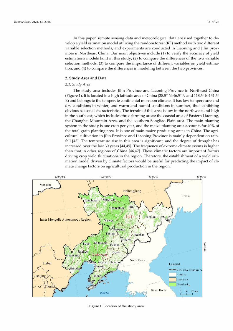
The study area includes Jilin Province and Liaoning Province in Northeast China

(Figure 1). It is located in a high latitude area of China (38.5° N-46.5° N and 118.5° E-131.5°

E) and belongs to the temperate continental monsoon climate. It has low temperature and

dry conditions in winter, and warm and humid conditions in summer, thus exhibiting

obvious seasonal characteristics. The terrain of this area is low in the northwest and high

in the southeast, which includes three farming areas: the coastal area of Eastern Liaoning,

the Changbai Mountain Area, and the southern Songliao Plain area. The main planting

system in the study is one crop per year, and the maize planting area accounts for 40% of

the total grain planting area. It is one of main maize producing areas in China. The agri-

cultural cultivation in Jilin Province and Liaoning Province is mainly dependent on rain-

fall [43]. The temperature rise in this area is significant, and the degree of drought has

increased over the last 30 years [44,45]. The frequency of extreme climate events is higher

than that in other regions of China [46,47]. These climatic factors are important factors

driving crop yield fluctuations in the region. Therefore, the establishment of a yield esti-

mation model driven by climate factors would be useful for predicting the impact of cli-

mate change factors on agricultural production in the region.

Figure 1. Location of the study area.

Remote Sens. 2021, 13, 2016 4 of 26

2.2. Data

The data used in this study mainly include meteorological reanalysis data, remote

sensing data, and statistical data (Table 1). The meteorological reanalysis data were taken

from the ERA5 dataset of the European Center for Medium-Term Weather Forecast

(ECMWF 2017). The total precipitation of ERA5 monthly averaged data and the 2 m tem-

perature of ERA5 hourly data were used in this study. The spatial resolution of the data

is 0.25°, and the time series covers the period from 1979 to 2018 [48]. The GPP (gross pri-

mary production) data were obtained from the National Science and Technology Basic

Conditions Platform-National Earth System Science Data Sharing Service Platform [49],

which provides GPP data with a resolution of 0.05° from 1982 to 2018 with a temporal

resolution of 8 d. This data set was estimated by the EC-LUE model [50], and the verifica-

tion results of the data set showed that its simulation capability exceeded that of the

MODIS-GPP product. The NDVI data, which has a spatial resolution of 0.05° from 1981

to 2018 on a time scale of 1 d, were obtained from the long time series AVH13C1 dataset

of the LTDR project [51]. The Chinese land use and land cover data at a 1 km resolution

were provided by the Resource and Environmental Science Data Center of the Chinese

Academy of Sciences (http://www.resdc.cn). This dataset was used to extract the range of

cultivated land. The statistical data mainly included the time series maize yield at the mu-

nicipal level (1996–2018 in Jilin Province and 1997–2018 in Liaoning Province) and agri-

cultural disaster statistics from 1990 to 2016 provided by the China Bureau of Statistics, as

well as crop phenological calendar from the planting management department of the Min-

istry of Agriculture.

Table 1. Data sources and characteristics.

Data Data Source Spatial Resolution Temporal Resolution

Meteorological

reanalysis data

Total

precipitation

ERA5 dataset of the European Center for

Medium-Term Weather Forecast

(ECMWF 2017)

0.25° Monthly

2 m

temperature ECMWF 2017 0.25° Hourly

Remote sensing

data

Gross primary

production

National Science and Technology Basic

Conditions Platform-National Earth System

Science Data Sharing Service Platform

0.05° 8 d

NDVI AVH13C1 dataset of the LTDR project 0.05° 1 d

Land use and

land cover data

Resource and Environmental Science Data

Center of the Chinese Academy of Sciences 1 km -

Statistical data

Maize yield China Bureau of Statistics Municipality Yearly

Agricultural

disaster

statistics

China Bureau of Statistics Province Yearly

3. Methodology

3.1. Input Variable Calculation

3.1.1. Calculation of Technical Yield

Grain yield is affected by many factors, including natural factors and nonnatural fac-

tors. Climate is the most important natural factor, as it is constantly fluctuating. Nonnat-

ural factors such as cultivation techniques and field management strategies have im-

proved over time. Therefore, the annual crop yield per unit area (Y ), which is defined as

the average amount of agricultural products harvested per unit of land area, can be di-

vided into two parts: climatic yield ( wY ) and trend yield ( tY ) (Equation (1)). Climatic yield

Remote Sens. 2021, 13, 2016 5 of 26

is determined by short-term climate variations, while the trend yield, which is also re-

ferred to as the technical yield, is influenced by long-term factors.

� = �� + �� (1)

There are many methods used to calculate the technical yield [52]. The most com-

monly used methods include the moving average method, HP filtering method [53], and

exponential smoothing method [54]. We used these three methods to separate the tech-

nical yield from the historical actual yield and then used the historical actual yield minus

the technical yield to calculate the climate yield. We calculated the correlation between

the climate yield derived from the three methods and the area of cultivated land suffered

by disaster. The climate yield with the highest correlation and the corresponding technical

yield were selected as the final calculation results. The correlation here was calculated

using the gray correlation analysis. Gray correlation analysis judges the correlation degree

between variables according to the degree of geometric similarity of the time series curve,

focuses on the consistency of the change trends among variables and is not limited by the

size and distribution of samples [55]. Through the above method, based on municipal-

level corn yield data of Jilin Province from 1996 to 2018 and Liaoning Province from 1997

to 2018, the technical yield and climate yield of the corresponding period were obtained.

3.1.2. Calculation of Agrometeorological Index

As a crop with high water requirements, maize is sensitive to water deficiency, and

the effects of drought during different growth stages on maize production differ [56].

Eighty-five percent of the corn planting areas in the study area are rain fed [43,57–59], and

drought occurs frequently during the maize growth period [60–62]. The standardized pre-

cipitation index (SPI) [63] is a commonly used drought monitoring index and has the ad-

vantage of multitemporal characteristics. The growth period of maize in the study area

lasts from April to September. To reflect the effects of drought on maize growth at differ-

ent times, SPI indexes with a two-month scale in May (SPI2-5), July (SPI2-7) and Septem-

ber (SPI2-9) were selected to represent drought conditions during the early, middle, and

late growth stages of maize, respectively. For each study year, we first calculated the SPI2-

5, SPI2-7, and SPI2-9 values iteratively for each grid; then, for each SPI index, we calcu-

lated its average value within the cultivated land area of each municipal administrative

region and used it as a candidate independent variable to participate in the construction

of the subsequent production estimation model.

Temperature is also an important climatic factor affecting maize production. The

suitable growth temperature of maize ranges from 10 to 30 °C [64]. During the growth

period, with increasing temperature, the yield of maize will increase; however, when the

temperature exceeds a certain threshold, temperature will have an obvious negative effect

on maize production [65–68]. Therefore, we calculated the extreme degree-day (EDD) and

accumulated temperature above 10 °C (AAT) to reflect the impact of temperature on

maize production. EDD was calculated as follows:

��� = � ���

�

���

/24 (2)

��� = �0

�� − ����

����

�� < ����

�� ≥ ���� (3)

In Equations (2) and (3), � is the number of hours within a certain period of time,

�� is the actual temperature at h-th hour, and ���� is the high temperature threshold. We

chose 30 °C as the threshold.

For each study year, we first calculated the EDD and AAT for each grid throughout

the whole growing season (from April to September) and each for month in the whole

growing season. The EDD from April to September was recorded as EDD4, EDD5, EDD6,

EDD7, EDD8, and EDD9, and the EDD of the whole growing season was recorded as

EDD4-9. Similarly, the AAT from April to September was recorded as AAT4, AAT5,

AAT6, AAT7, AAT8, and AAT9, and the AAT of the whole growing season was recorded

Remote Sens. 2021, 13, 2016 6 of 26

as AAT4-9. Then, for each EDD (AAT) index, we calculated its average value in the culti-

vated land area of each municipal administrative region and used it as a candidate inde-

pendent variable to participate in the construction of the subsequent yield estimation

model.

3.1.3. Calculation of NDVI and GPP Anomalies

In this study, the AVH13C1 daily scale NDVI from 1990 to 2018 was merged into a

monthly NDVI dataset by using the maximum composite method (MVC), and then the

residual noise in the time series was removed by S-G filtering to obtain high-quality NDVI

data [69]. After that, NDVI anomalies were obtained according to the method proposed

by Papagiannopoulou et al. [70].

First, the overall trend of NDVI values in each pixel over the study years was re-

moved, meaning that the time series was taken as the independent variable �, and the

NDVI value of the corresponding pixel in the time series was taken as the dependent var-

iable �� for linear fitting (Equation (4)). The difference between the NDVI value y and

the NDVI fitted value �� was the detrended NDVI value ��� (Equation (5)).

�� = � + �� (4)

��� = y − �� (5)

Second, the seasonal component of the NDVI values after detrending was calculated.

Assuming that the data were evenly distributed in the time series, the monthly mean value

of NDVI in each pixel was taken as the NDVI value in the seasonal period (����).

Third, the NDVI anomaly ��� was calculated by taking the detrended NDVI value

��� minus the NDVI value in the seasonal period (����).

��� = ��� − ���� (6)

For the monthly NDVI data collected from 1981 to 2018, the corresponding monthly

NDVI anomaly (NDVIa) was calculated for each grid using the method mentioned above.

Then, for each study year, we calculated the average NDVIa value in the cultivated land

area of each municipal administrative region for the whole growing season (from April to

September) and for each month in the whole growing season. The average NDVIa from

April to September was recorded as NDVIa4, NDVIa5, NDVIa6, NDVIa7, NDVIa8, and

NDVIa9, and the average NDVIa of the whole growing season was recorded as NDVIa4-

9. Using the same method, we calculated the monthly GPP anomaly (GPPa) for each grid

and then further calculated the average value of GPPa in the cultivated land area of each

municipal administrative region for the whole growing season (from April to September)

and for each month during the whole growing season. The average GPPa from April to

September was recorded as GPPa4, GPPa5, GPPa6, GPPa7, GPPa8, and GPPa9, and the

average GPPa of the whole growing season was recorded as GPPa4-9.

3.2. Model Building Process

Taking the municipal level corn yield data of Jilin Province from 1996 to 2018 and

Liaoning Province from 1997 to 2018 as a dependent variable, the technical yield �� of the

corresponding years in each municipal administrative region as a fixed independent var-

iable, and GPPa variables, NDVIa variables, SPI variables, EDD variables, and AAT vari-

ables as candidate independent variables, two methods were used to select the independ-

ent variables of the input model from the candidate independent variables, and then the

yield estimation models were established by the RF with the fixed independent variable

and selected candidate independent variables as input. The accuracy of the yield estima-

tion model established by the two variable selection methods was compared, and the dif-

ferences in the selected variables were analyzed. It should be emphasized here that the

fixed variable (��) acted as an input variable in each modeling process. GPPa variables

included GPPa4, GPPa5, GPPa6, GPPa7, GPPa8, GPPa9, and GPPa4-9. NDVIa variables

included NDVIa4, NDVIa5, NDVIa6, NDVIa7, NDVIa8, NDVIa9, and NDVIa4-9. SPI var-

iables included SPI2-5, SPI2-7, and SPI2-9. EDD variables included EDD4, EDD5, EDD6,

Remote Sens. 2021, 13, 2016 7 of 26

EDD7, EDD8, EDD9, and EDD4-9. AAT variables included AAT4, AAT5, AAT6, AAT7,

AAT8, AAT9, and AAT4-9. Therefore, there were 31 candidate independent variables in

total. The random forest regression under scikit learn in Python is used to train the model.

In the process of RF construction, the number of regression trees ‘n_estimators’ and the

number of randomly selected features per decision tree ‘max_feature’ are important pa-

rameters affecting the prediction ability of the RF model, and max_feature should be less

than the number of variables in the model (n_features). The optimal parameters of the RF

model were selected using the grid search method in which max_feature ranged from 1

to n_features with a step size of 2, and n_estimators ranged from 80 to 200 with a step size

of 10. By comparing the out-of-bag data errors of the models with different combinations

of parameters, the max_feature and n_estimators values corresponding to the minimum

out-of-bag data errors were defined as the optimal parameters. Eighty percent of the com-

plete dataset was randomly selected to train each model, and the remaining data were

used to validate the model. The specific processes of the two variable selection methods

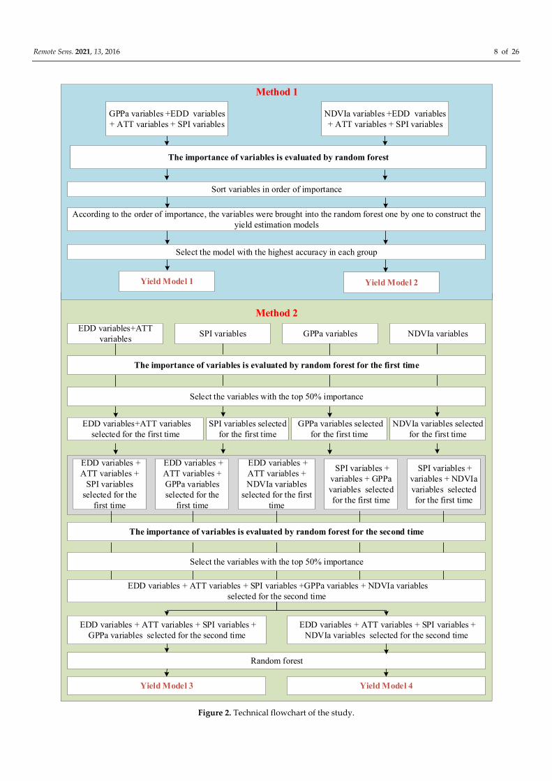
are shown in Figure 2.

Remote Sens. 2021, 13, 2016 8 of 26

Method 2

Method 1

The importance of variables is evaluated by random forest

EDD variables + ATT variables + SPI variables +GPPa variables + NDVIa variables selected for the second time

Random forest

Select the variables with the top 50% importance

EDD variables + ATT variables +

SPI variables selected for the

first time

EDD variables + ATT variables + GPPa variables selected for the

first time

EDD variables + ATT variables + NDVIa variables

selected for the first time

SPI variables + variables + GPPa variables selected for the first time

SPI variables + variables + NDVIa variables selected for the first time

The importance of variables is evaluated by random forest for the first time

Select the variables with the top 50% importance

EDD variables + ATT variables + SPI variables + GPPa variables selected for the second time

EDD variables + ATT variables + SPI variables + NDVIa variables selected for the second time

Sort variables in order of importance

Select the model with the highest accuracy in each group

According to the order of importance, the variables were brought into the random forest one by one to construct the yield estimation models

GPPa variables +EDD variables + ATT variables + SPI variables

NDVIa variables +EDD variables + ATT variables + SPI variables

Yield Model 1 Yield Model 2

EDD variables+ATT variables

SPI variables GPPa variables NDVIa variables

EDD variables+ATT variables selected for the first time

SPI variables selected for the first time

GPPa variables selected for the first time

NDVIa variables selected for the first time

The importance of variables is evaluated by random forest for the second time

Yield Model 3 Yield Model 4

Figure 2. Technical flowchart of the study.

Remote Sens. 2021, 13, 2016 9 of 26

In the first method, the importance of the candidate independent variables was eval-

uated by the random forest method. We first divided the candidate variables into two

groups: the GPP group and the NDVI group. The GPP group included GPPa variables,

EDD variables, ATT variables, and SPI variables; the NDVI group included NDVIa vari-

ables, EDD variables, ATT variables, and SPI variables. Each group had 24 variables. Ac-

cording to the importance of variables ranked by the random forest method, the variables

were iteratively added to establish the best yield estimation model. The most important

variable was added first, and then the next important variable was added until all varia-

bles were added to the model. In this way, for each group of variables, we established 24

yield estimation models, verified the accuracy of each production estimation model, and

selected the model with the highest accuracy as the final yield estimation model corre-

sponding to this group of variables. To facilitate the subsequent analysis, we defined the

final yield estimation model for the GPP group as Yield Model 1 and the final yield esti-

mation model for the NDVI group as Yield Model 2.

In the second method, modeling variables were selected by a two-stage importance

evaluation method. We first divided the candidate variables into four groups: a tempera-

ture group (including EDD variables and ATT variables), an SPI group (including SPI

variables), a GPPa group (including GPPa variables), and a NDVIa group (including

NDVIa variables). For each group, we evaluated the importance of the candidate variables

using the random forest method and selected the variables constituting the top 50% im-

portance from each group to form new variable groups. Then, the new temperature group

(including EDD variables and ATT variables), SPI group, GPPa group, and NDVIa group

were combined in pairs to form 5 groups: temperature group variables + SPI variables;

temperature group variables + GPPa variables; temperature group variables + NDVIa var-

iables; SPI variables + GPPa variables; and SPI variables + NDVIa variables. For each

group, we reevaluated the importance of the candidate variables by the random forest

method and selected the variables constituting the top 50% importance from each group

to obtain the final candidate independent variables. Then, we divided the final candidate

independent variables into two groups: the GPP group and the NDVI group. The GPP

group included temperature group variables, SPI variables, and GPPa variables selected

for the second time; the NDVI group included temperature group variables, SPI variables,

and NDVIa variables selected for the second time. Finally, we built two yield estimation

models (referred to as Yield Models 3 and 4) based on the two group variables using the

random forest method.

3.3. Model Validation

The performances of the yield estimation models were evaluated by using three val-

idation measurements: the mean absolute relative deviation (MARE), coefficient of deter-

mination (R2) and the Lin’s concordance correlation coefficient (CCC):

���� =1

��

|�� − ��|

��

�

���

(7)

�� =

⎝

⎛�∑ (�� − �̄)(�� − �� )�

���

�∑ (�� − �̄)����� �∑ (�� − �� )��

��� ⎠

⎞

�

(8)

CCC =2���

(�� − �̅)� + �� + ��

(9)

where ir and iR refer to the reported and estimated maize yield in year i ; r and R

are the mean values of the reported and estimated values of maize yield; �� and �� are

Remote Sens. 2021, 13, 2016 10 of 26

the variance of the reported and estimated values of maize yield; n is the number of sam-

ples, ��� is the covariance between the reported and estimated values of maize yield.

MARE reflects the credibility of an estimation. The CCC measures the agreement between

two variables. The model results become increasingly more accurate as R2 and CCC ap-

proach 1 and MARE approaches 0.

4. Results

4.1. Trend Yield

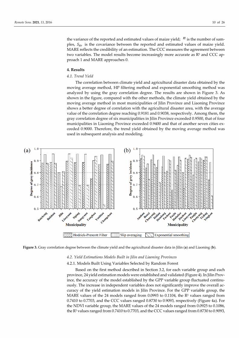
The correlation between climate yield and agricultural disaster data obtained by the

moving average method, HP filtering method and exponential smoothing method was

analyzed by using the gray correlation degree. The results are shown in Figure 3. As

shown in the figure, compared with the other methods, the climate yield obtained by the

moving average method in most municipalities of Jilin Province and Liaoning Province

shows a better degree of correlation with the agricultural disaster area, with the average

value of the correlation degree reaching 0.9181 and 0.9038, respectively. Among them, the

gray correlation degree of six municipalities in Jilin Province exceeded 0.9500, that of four

municipalities in Liaoning Province exceeded 0.9400 and that of another seven cities ex-

ceeded 0.9000. Therefore, the trend yield obtained by the moving average method was

used in subsequent analysis and modeling.

Figure 3. Gray correlation degree between the climate yield and the agricultural disaster data in Jilin (a) and Liaoning (b).

4.2. Yield Estimations Models Built in Jilin and Liaoning Provinces

4.2.1. Models Built Using Variables Selected by Random Forest

Based on the first method described in Section 3.2, for each variable group and each

province, 24 yield estimation models were established and validated (Figure 4). In Jilin Prov-

ince, the accuracy of the model established by the GPP variable group fluctuated continu-

ously. The increase in independent variables does not significantly improve the overall ac-

curacy of the yield estimation models in Jilin Province. For the GPP variable group, the

MARE values of the 24 models ranged from 0.0993 to 0.1104, the R2 values ranged from

0.7410 to 0.7703, and the CCC values ranged 0.8730 to 0.9093, respectively (Figure 4a). For

the NDVI variable group, the MARE values of the 24 models ranged from 0.0925 to 0.1086,

the R2 values ranged from 0.7410 to 0.7703, and the CCC values ranged from 0.8730 to 0.9093,

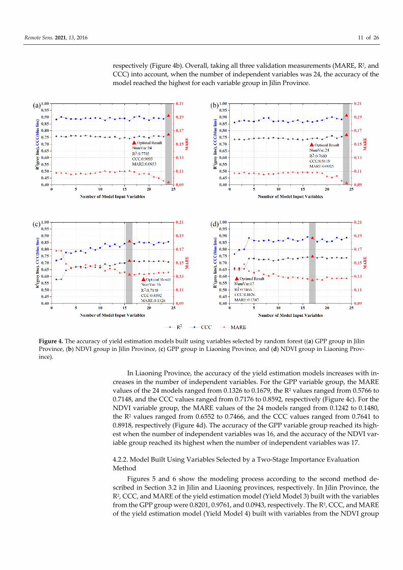
Remote Sens. 2021, 13, 2016 11 of 26

respectively (Figure 4b). Overall, taking all three validation measurements (MARE, R2, and

CCC) into account, when the number of independent variables was 24, the accuracy of the

model reached the highest for each variable group in Jilin Province.

Figure 4. The accuracy of yield estimation models built using variables selected by random forest ((a) GPP group in Jilin

Province, (b) NDVI group in Jilin Province, (c) GPP group in Liaoning Province, and (d) NDVI group in Liaoning Prov-

ince).

In Liaoning Province, the accuracy of the yield estimation models increases with in-

creases in the number of independent variables. For the GPP variable group, the MARE

values of the 24 models ranged from 0.1326 to 0.1679, the R2 values ranged from 0.5766 to

0.7148, and the CCC values ranged from 0.7176 to 0.8592, respectively (Figure 4c). For the

NDVI variable group, the MARE values of the 24 models ranged from 0.1242 to 0.1480,

the R2 values ranged from 0.6552 to 0.7466, and the CCC values ranged from 0.7641 to

0.8918, respectively (Figure 4d). The accuracy of the GPP variable group reached its high-

est when the number of independent variables was 16, and the accuracy of the NDVI var-

iable group reached its highest when the number of independent variables was 17.

4.2.2. Model Built Using Variables Selected by a Two-Stage Importance Evaluation

Method

Figures 5 and 6 show the modeling process according to the second method de-

scribed in Section 3.2 in Jilin and Liaoning provinces, respectively. In Jilin Province, the

R2, CCC, and MARE of the yield estimation model (Yield Model 3) built with the variables

from the GPP group were 0.8201, 0.9761, and 0.0943, respectively. The R2, CCC, and MARE

of the yield estimation model (Yield Model 4) built with variables from the NDVI group

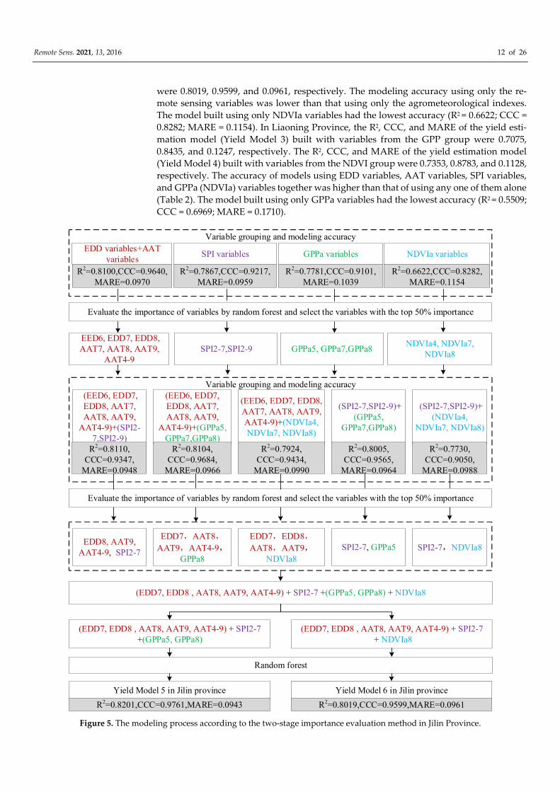
Remote Sens. 2021, 13, 2016 12 of 26

were 0.8019, 0.9599, and 0.0961, respectively. The modeling accuracy using only the re-

mote sensing variables was lower than that using only the agrometeorological indexes.

The model built using only NDVIa variables had the lowest accuracy (R2 = 0.6622; CCC =

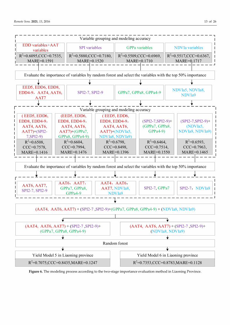
0.8282; MARE = 0.1154). In Liaoning Province, the R2, CCC, and MARE of the yield esti-

mation model (Yield Model 3) built with variables from the GPP group were 0.7075,

0.8435, and 0.1247, respectively. The R2, CCC, and MARE of the yield estimation model

(Yield Model 4) built with variables from the NDVI group were 0.7353, 0.8783, and 0.1128,

respectively. The accuracy of models using EDD variables, AAT variables, SPI variables,

and GPPa (NDVIa) variables together was higher than that of using any one of them alone

(Table 2). The model built using only GPPa variables had the lowest accuracy (R2 = 0.5509;

CCC = 0.6969; MARE = 0.1710).

Variable grouping and modeling accuracy

Variable grouping and modeling accuracy

(EDD7, EDD8 , AAT8, AAT9, AAT4-9) + SPI2-7 +(GPPa5, GPPa8) + NDVIa8

Random forest

(EED6, EDD7, EDD8, AAT7, AAT8, AAT9,

AAT4-9)+(SPI2-7,SPI2-9)

(EED6, EDD7, EDD8, AAT7, AAT8, AAT9,

AAT4-9)+(GPPa5, GPPa7,GPPa8)

(EED6, EDD7, EDD8, AAT7, AAT8, AAT9, AAT4-9)+(NDVIa4, NDVIa7, NDVIa8)

(SPI2-7,SPI2-9)+ (GPPa5,

GPPa7,GPPa8)

(SPI2-7,SPI2-9)+ (NDVIa4,

NDVIa7, NDVIa8)

Evaluate the importance of variables by random forest and select the variables with the top 50% importance

(EDD7, EDD8 , AAT8, AAT9, AAT4-9) + SPI2-7 +(GPPa5, GPPa8)

(EDD7, EDD8 , AAT8, AAT9, AAT4-9) + SPI2-7 + NDVIa8

EDD variables+AAT variables

SPI variables GPPa variables NDVIa variables

EED6, EDD7, EDD8, AAT7, AAT8, AAT9,

AAT4-9SPI2-7,SPI2-9 GPPa5, GPPa7,GPPa8

NDVIa4, NDVIa7, NDVIa8

Evaluate the importance of variables by random forest and select the variables with the top 50% importance

Yield Model 5 in Jilin province Yield Model 6 in Jilin province

EDD8, AAT9, AAT4-9, SPI2-7

EDD7，AAT8，

AAT9，AAT4-9，GPPa8

EDD7，EDD8，

AAT8，AAT9，NDVIa8

SPI2-7, GPPa5 SPI2-7，NDVIa8

R2=0.8100,CCC=0.9640,MARE=0.0970

R2=0.7867,CCC=0.9217,MARE=0.0959

R2=0.7781,CCC=0.9101,MARE=0.1039

R2=0.6622,CCC=0.8282,MARE=0.1154

R2=0.8110,CCC=0.9347,

MARE=0.0948

R2=0.8104,CCC=0.9684,

MARE=0.0966

R2=0.7924,CCC=0.9434,

MARE=0.0990

R2=0.8005,CCC=0.9565,

MARE=0.0964

R2=0.7730,CCC=0.9050,

MARE=0.0988

R2=0.8201,CCC=0.9761,MARE=0.0943 R2=0.8019,CCC=0.9599,MARE=0.0961

Figure 5. The modeling process according to the two-stage importance evaluation method in Jilin Province.

Remote Sens. 2021, 13, 2016 13 of 26

Variable grouping and modeling accuracy

Variable grouping and modeling accuracy

(AAT4, AAT6, AAT7) + (SPI2-7 ,SPI2-9)+(GPPa7, GPPa8, GPPa4-9) + (NDVIa8, NDVIa9)

Random forest

( EED5, EDD6,

EDD8, EDD4-9，AAT4, AAT6, AAT7)+(SPI2-

7,SPI2-9)

(EED5, EDD6,

EDD8, EDD4-9，AAT4, AAT6,

AAT7)+(GPPa7, GPPa8, GPPa4-9)

( EED5, EDD6,

EDD8, EDD4-9，AAT4, AAT6,

AAT7)+(NDVIa5, NDVIa8, NDVIa9)

(SPI2-7,SPI2-9)+ (GPPa7, GPPa8,

GPPa4-9)

(SPI2-7,SPI2-9)+ (NDVIa5,

NDVIa8, NDVIa9)

Evaluate the importance of variables by random forest and select the variables with the top 50% importance

(AAT4, AAT6, AAT7) + (SPI2-7 ,SPI2-9)+(GPPa7, GPPa8, GPPa4-9)

(AAT4, AAT6, AAT7) + (SPI2-7 ,SPI2-9)+ (NDVIa8, NDVIa9)

EDD variables+AAT variables

SPI variables GPPa variables NDVIa variables

EED5, EDD6, EDD8,

EDD4-9，AAT4, AAT6, AAT7

SPI2-7, SPI2-9 GPPa7, GPPa8, GPPa4-9NDVIa5, NDVIa8,

NDVIa9

Evaluate the importance of variables by random forest and select the variables with the top 50% importance

Yield Model 5 in Liaoning province Yield Model 6 in Liaoning province

AAT6, AAT7, SPI2-7, SPI2-9

AAT6，AAT7，GPPa7, GPPa8,

GPPa4-9

AAT4，AAT6，AAT7, NDVIa8,

NDVIa9

SPI2-7, GPPa7 SPI2-7，NDVIa8

R2=0.6095,CCC=0.7535,MARE=0.1591

R2=0.5880,CCC=0.7180,MARE=0.1520

R2=0.5509,CCC=0.6969,MARE=0.1710

R2=0.5517,CCC=0.6367,MARE=0.1717

R2=0.6508,CCC=0.7578,

MARE=0.1416

R2=0.6604,CCC=0.7994,

MARE=0.1476

R2=0.6798,CCC=0.8498,

MARE=0.1396

R2=0.6464,CCC=0.7514,

MARE=0.1550

R2=0.6593,CCC=0.7963,

MARE=0.1465

R2=0.7075,CCC=0.8435,MARE=0.1247 R2=0.7353,CCC=0.8783,MARE=0.1128

Figure 6. The modeling process according to the two-stage importance evaluation method in Liaoning Province.

Remote Sens. 2021, 13, 2016 14 of 26

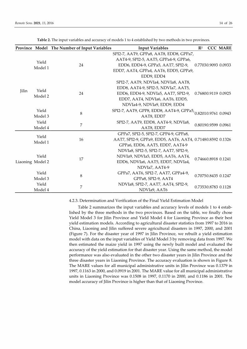
Table 2. The input variables and accuracy of models 1 to 4 established by two methods in two provinces.

Province Model The Number of Input Variables Input Variables R2 CCC MARE

Jilin

Yield

Model 1 24

SPI2-7, AAT9, GPPa8, AAT8, EDD8, GPPa7,

AAT4-9, SPI2-5, AAT5, GPPa4-9, GPPa6,

EDD6, EDD4-9, GPPa5, AAT7, SPI2-9,

EDD7, AAT4, GPPa4, AAT6, EDD5, GPPa9,

EDD9, EDD4

0.7703 0.9093 0.0933

Yield

Model 2 24

SPI2-7, AAT9, NDVIa4, NDVIa8, AAT8,

EDD8, AAT4-9, SPI2-5, NDVIa7, AAT5,

EDD6, EDD4-9, NDVIa5, AAT7, SPI2-9,

EDD7, AAT4, NDVIa6, AAT6, EDD5,

NDVIa4-9, NDVIa9, EDD9, EDD4

0.7680 0.9119 0.0925

Yield

Model 3 8

SPI2-7, AAT9, GPP8, EDD8, AAT4-9, GPPa5,

AAT8, EDD7 0.8201 0.9761 0.0943

Yield

Model 4 7

SPI2-7, AAT9, EDD8, AAT4-9, NDVIa8,

AAT8, EDD7 0.8019 0.9599 0.0961

Liaoning

Yield

Model 1 16

GPPa7, SPI2-5, SPI2-7, GPP4-9, GPPa8,

AAT7, SPI2-9, GPPa9, EDD5, AAT6, AAT4,

GPPa6, EDD6, AAT5, EDD7, AAT4-9

0.7148 0.8592 0.1326

Yield

Model 2 17

NDVIa8, SPI2-5, SPI2-7, AAT7, SPI2-9,

NDVIa9, NDVIa5, EDD5, AAT6, AAT4,

EDD6, NDVIa6, AAT5, EDD7, NDVIa4,

NDVIa7, AAT4-9

0.7466 0.8918 0.1241

Yield

Model 3 8

GPPa7, AAT6, SPI2-7, AAT7, GPPa4-9,

GPPa8, SPI2-9, AAT4 0.7075 0.8435 0.1247

Yield

Model 4 7

NDVIa8, SPI2-7, AAT7, AAT4, SPI2-9,

NDVIa9, AAT6 0.7353 0.8783 0.1128

4.2.3. Determination and Verification of the Final Yield Estimation Model

Table 2 summarizes the input variables and accuracy levels of models 1 to 4 estab-

lished by the three methods in the two provinces. Based on the table, we finally chose

Yield Model 3 for Jilin Province and Yield Model 4 for Liaoning Province as their best

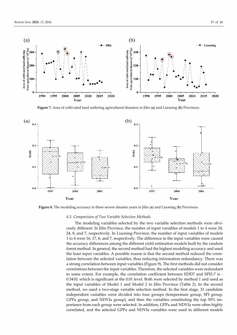
yield estimation models. According to agricultural disaster statistics from 1997 to 2016 in

China, Liaoning and Jilin suffered severe agricultural disasters in 1997, 2000, and 2001

(Figure 7). For the disaster year of 1997 in Jilin Province, we rebuilt a yield estimation

model with data on the input variables of Yield Model 3 by removing data from 1997. We

then estimated the maize yield in 1997 using the newly built model and evaluated the

accuracy of the yield estimation for that disaster year. Using the same method, the model

performance was also evaluated in the other two disaster years in Jilin Province and the

three disaster years in Liaoning Province. The accuracy evaluation is shown in Figure 8.

The MARE values for all municipal administrative units in Jilin Province was 0.1379 in

1997, 0.1163 in 2000, and 0.0919 in 2001. The MARE value for all municipal administrative

units in Liaoning Province was 0.1508 in 1997, 0.1170 in 2000, and 0.1186 in 2001. The

model accuracy of Jilin Province is higher than that of Liaoning Province.

Remote Sens. 2021, 13, 2016 15 of 26

Figure 7. Area of cultivated land suffering agricultural disasters in Jilin (a) and Liaoning (b) Provinces.

Figure 8. The modeling accuracy in three severe disaster years in Jilin (a) and Liaoning (b) Provinces.

4.3. Comparision of Two Variable Selection Methods

The modeling variables selected by the two variable selection methods were obvi-

ously different. In Jilin Province, the number of input variables of models 1 to 4 were 24,

24, 8, and 7, respectively. In Liaoning Province, the number of input variables of models

1 to 4 were 16, 17, 8, and 7, respectively. The difference in the input variables were caused

the accuracy differences among the different yield estimation models built by the random

forest method. In general, the second method had the highest modeling accuracy and used

the least input variables. A possible reason is that the second method reduced the corre-

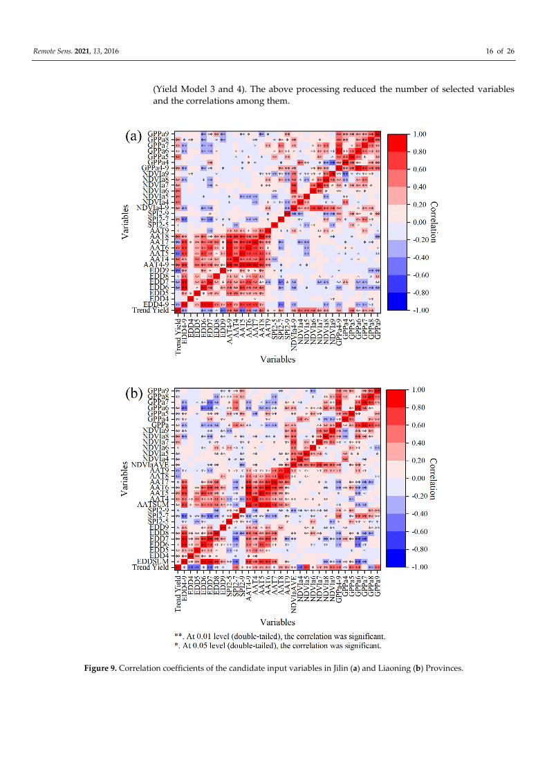
lation between the selected variables, thus reducing information redundancy. There was

a strong correlation between input variables (Figure 9). The first methods did not consider

correlations between the input variables. Therefore, the selected variables were redundant

to some extent. For example, the correlation coefficient between EDD7 and SPI2-7 is -

0.5410, which is significant at the 0.01 level. Both were selected by method 1 and used as

the input variables of Model 1 and Model 2 in Jilin Province (Table 2). In the second

method, we used a two-stage variable selection method. In the first stage, 31 candidate

independent variables were divided into four groups (temperature group, SPI group,

GPPa group, and NDVIa group), and then the variables constituting the top 50% im-

portance from each group were selected. In addition, GPPa and NDVIa were often highly

correlated, and the selected GPPa and NDVIa variables were used in different models

Remote Sens. 2021, 13, 2016 16 of 26

(Yield Model 3 and 4). The above processing reduced the number of selected variables

and the correlations among them.

Figure 9. Correlation coefficients of the candidate input variables in Jilin (a) and Liaoning (b) Provinces.

Remote Sens. 2021, 13, 2016 17 of 26

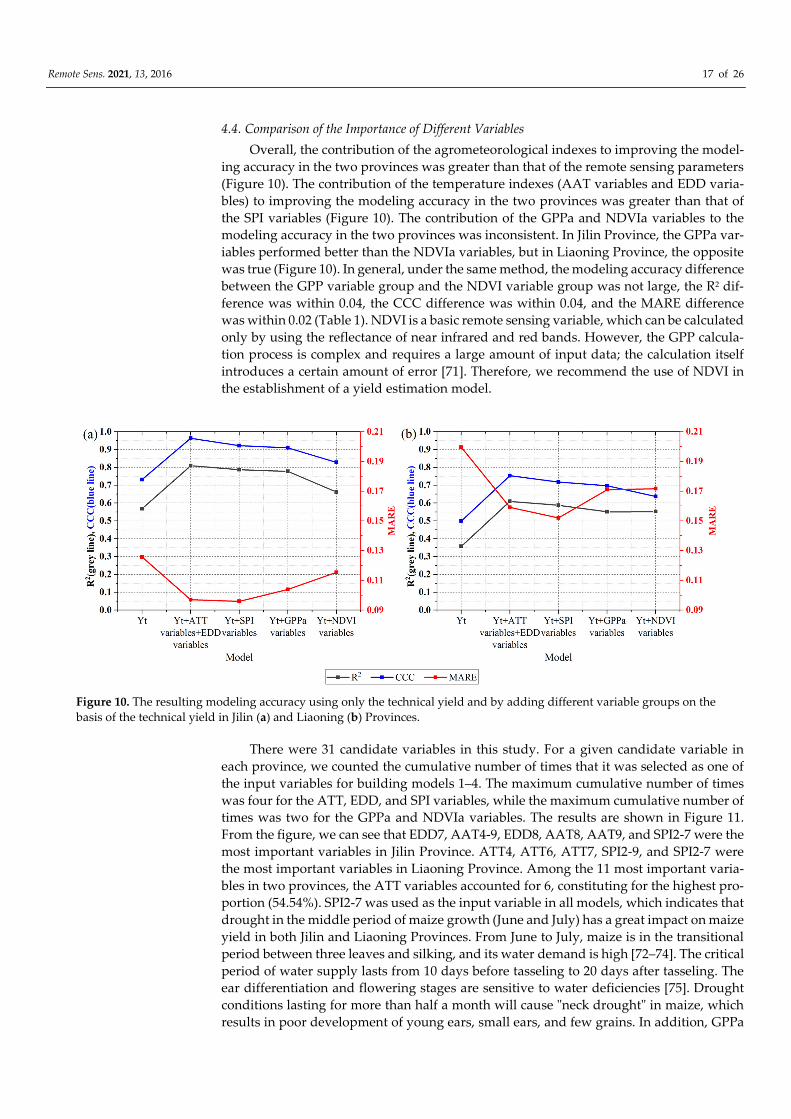
4.4. Comparison of the Importance of Different Variables

Overall, the contribution of the agrometeorological indexes to improving the model-

ing accuracy in the two provinces was greater than that of the remote sensing parameters

(Figure 10). The contribution of the temperature indexes (AAT variables and EDD varia-

bles) to improving the modeling accuracy in the two provinces was greater than that of

the SPI variables (Figure 10). The contribution of the GPPa and NDVIa variables to the

modeling accuracy in the two provinces was inconsistent. In Jilin Province, the GPPa var-

iables performed better than the NDVIa variables, but in Liaoning Province, the opposite

was true (Figure 10). In general, under the same method, the modeling accuracy difference

between the GPP variable group and the NDVI variable group was not large, the R2 dif-

ference was within 0.04, the CCC difference was within 0.04, and the MARE difference

was within 0.02 (Table 1). NDVI is a basic remote sensing variable, which can be calculated

only by using the reflectance of near infrared and red bands. However, the GPP calcula-

tion process is complex and requires a large amount of input data; the calculation itself

introduces a certain amount of error [71]. Therefore, we recommend the use of NDVI in

the establishment of a yield estimation model.

Figure 10. The resulting modeling accuracy using only the technical yield and by adding different variable groups on the

basis of the technical yield in Jilin (a) and Liaoning (b) Provinces.

There were 31 candidate variables in this study. For a given candidate variable in

each province, we counted the cumulative number of times that it was selected as one of

the input variables for building models 1–4. The maximum cumulative number of times

was four for the ATT, EDD, and SPI variables, while the maximum cumulative number of

times was two for the GPPa and NDVIa variables. The results are shown in Figure 11.

From the figure, we can see that EDD7, AAT4-9, EDD8, AAT8, AAT9, and SPI2-7 were the

most important variables in Jilin Province. ATT4, ATT6, ATT7, SPI2-9, and SPI2-7 were

the most important variables in Liaoning Province. Among the 11 most important varia-

bles in two provinces, the ATT variables accounted for 6, constituting for the highest pro-

portion (54.54%). SPI2-7 was used as the input variable in all models, which indicates that

drought in the middle period of maize growth (June and July) has a great impact on maize

yield in both Jilin and Liaoning Provinces. From June to July, maize is in the transitional

period between three leaves and silking, and its water demand is high [72–74]. The critical

period of water supply lasts from 10 days before tasseling to 20 days after tasseling. The

ear differentiation and flowering stages are sensitive to water deficiencies [75]. Drought

conditions lasting for more than half a month will cause "neck drought" in maize, which

results in poor development of young ears, small ears, and few grains. In addition, GPPa

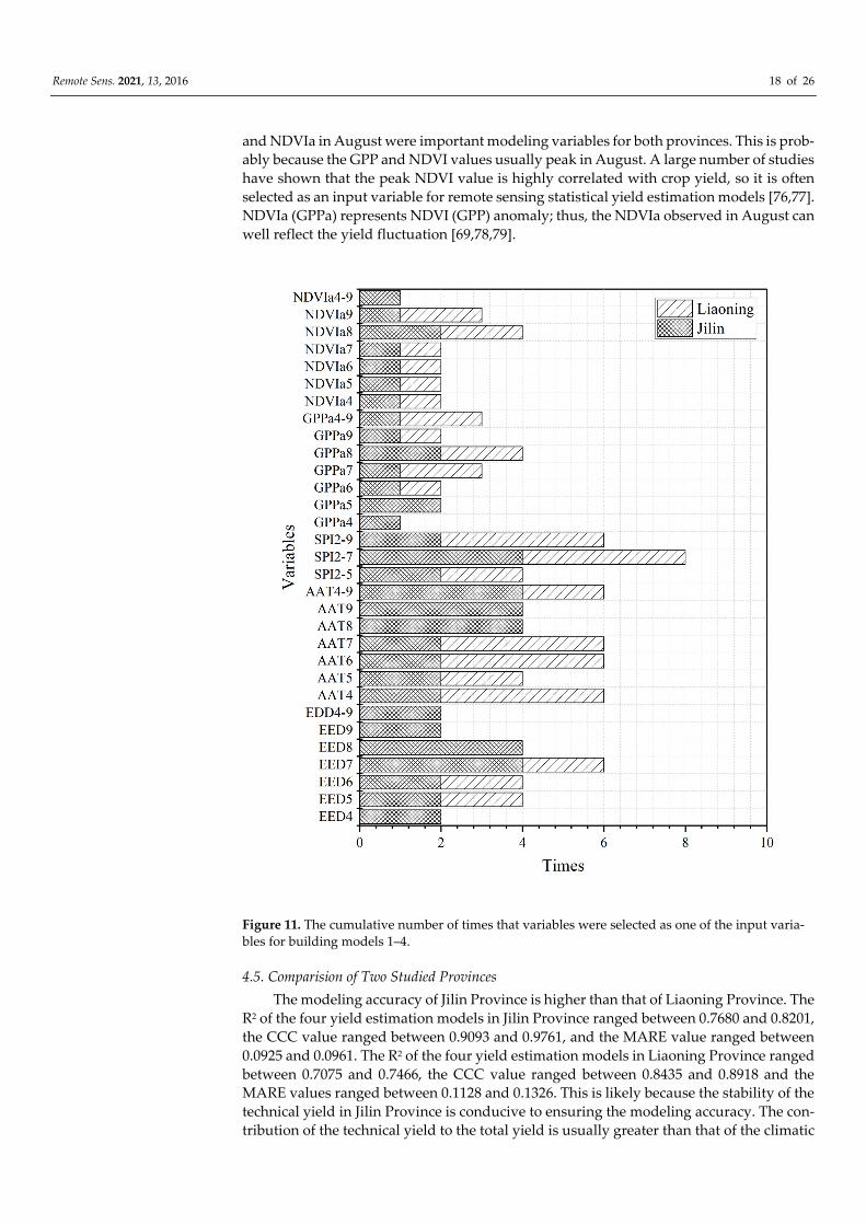
Remote Sens. 2021, 13, 2016 18 of 26

and NDVIa in August were important modeling variables for both provinces. This is prob-

ably because the GPP and NDVI values usually peak in August. A large number of studies

have shown that the peak NDVI value is highly correlated with crop yield, so it is often

selected as an input variable for remote sensing statistical yield estimation models [76,77].

NDVIa (GPPa) represents NDVI (GPP) anomaly; thus, the NDVIa observed in August can

well reflect the yield fluctuation [69,78,79].

Figure 11. The cumulative number of times that variables were selected as one of the input varia-

bles for building models 1–4.

4.5. Comparision of Two Studied Provinces

The modeling accuracy of Jilin Province is higher than that of Liaoning Province. The

R2 of the four yield estimation models in Jilin Province ranged between 0.7680 and 0.8201,

the CCC value ranged between 0.9093 and 0.9761, and the MARE value ranged between

0.0925 and 0.0961. The R2 of the four yield estimation models in Liaoning Province ranged

between 0.7075 and 0.7466, the CCC value ranged between 0.8435 and 0.8918 and the

MARE values ranged between 0.1128 and 0.1326. This is likely because the stability of the

technical yield in Jilin Province is conducive to ensuring the modeling accuracy. The con-

tribution of the technical yield to the total yield is usually greater than that of the climatic

Remote Sens. 2021, 13, 2016 19 of 26

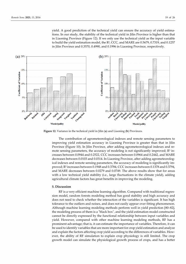
yield. A good prediction of the technical yield can ensure the accuracy of yield estima-

tions. In our study, the stability of the technical yield in Jilin Province is higher than that

in Liaoning Province (Figure 12). If we only use the technical yield as the input variable

to build the yield estimation model, the R2, CCC, and MARE are 0.5679, 0.7319, and 0.1257

in Jilin Province and 0.3570, 0.4990, and 0.1996 in Liaoning Province, respectively.

Figure 12. Variance in the technical yield in Jilin (a) and Liaoning (b) Provinces.

The contribution of agrometeorological indexes and remote sensing parameters to

improving yield estimation accuracy in Liaoning Province is greater than that in Jilin

Province (Figure 10). In Jilin Province, after adding agrometeorological indexes and re-

mote sensing parameters, the accuracy of modeling is not significantly improved; R2 in-

creases between 0.0944 and 0.2522, CCC increases between 0.0964 and 0.2442, and MARE

decreases between 0.0103 and 0.0314. In Liaoning Province, after adding agrometeorolog-

ical indexes and remote sensing parameters, the accuracy of modeling is significantly im-

proved; R2 increases between 0.1948 and 0.3784, CCC increases between 0.1378 and 0.3794,

and MARE decreases between 0.0279 and 0.0749. The above results show that for areas

with a low technical yield stability (i.e., large fluctuations in the climate yield), adding

agricultural climate factors has great benefits in improving the modeling.

5. Discussion

RF is a very efficient machine learning algorithm. Compared with traditional regres-

sion model, random forests modeling method has good stability and high accuracy and

does not need to check whether the interaction of the variables is significant. It has high

tolerance to the outliers and noises, and does not easily appear over fitting phenomenon.

Although machine learning modeling methods perform well in yield prediction [80–82],

the modeling process of them is a "black box", and the yield estimation model constructed

cannot be directly expressed by the functional relationship between input variables and

yield. However, compared with other machine learning modeling methods, RF has a

prominent advantage; that is, it can estimate the importance of variables. Therefore, it can

be used to identify variables that are more important for crop yield estimation and analyze

and explain the factors affecting crop yield according to the differences of variables. How-

ever, the ability of RF simulation to explain crop physiology is still limited. The crop

growth model can simulate the physiological growth process of crops, and has a better

Remote Sens. 2021, 13, 2016 20 of 26

mechanism [7,83]. The combination of machine learning and the crop growth model could

be a new direction for crop yield estimation [84].

We proposed a new strategy for the yield estimation model development in which

remote sensing indexes, agrometeorological indexes, and technical yield are used to-

gether, and modeling variables are selected by a two-stage importance evaluation

method. The new strategy was tested in two different provinces: Jilin and Liaoning. Alt-

hough both provinces are the main maize producing provinces, and located in Northeast

China, there are some differences between them. First, technical yield is the dominant

component of yield. It is also the most important modelling variable. The average coeffi-

cient of variation of maize technical yield during the study period was 8.94% in Jilin Prov-

ince and 10.86% in Liaoning Province (Figure 12), indicating the stability of the technical

yield in Jilin Province is higher than that in Liaoning Province. This makes the overall

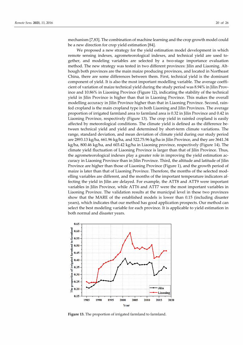
modelling accuracy in Jilin Province higher than that in Liaoning Province. Second, rain-

fed cropland is the main cropland type in both Liaoning and Jilin Provinces. The average

proportion of irrigated farmland area to farmland area is 0.32 in Jilin Province and 0.42 in

Liaoning Province, respectively (Figure 13). The crop yield in rainfed cropland is easily

affected by meteorological conditions. The climate yield is defined as the difference be-

tween technical yield and yield and determined by short-term climate variations. The

range, standard deviation, and mean deviation of climate yield during our study period

are 2893.13 kg/ha, 661.96 kg/ha, and 522.75.96 kg/ha in Jilin Province, and they are 3641.34

kg/ha, 800.46 kg/ha, and 603.42 kg/ha in Liaoning province, respectively (Figure 14). The

climate yield fluctuation of Liaoning Province is larger than that of Jilin Province. Thus,

the agrometeorological indexes play a greater role in improving the yield estimation ac-

curacy in Liaoning Province than in Jilin Province. Third, the altitude and latitude of Jilin

Province are higher than those of Liaoning Province (Figure 1), and the growth period of

maize is later than that of Liaoning Province. Therefore, the months of the selected mod-

elling variables are different, and the months of the important temperature indicators af-

fecting the yield in Jilin are delayed. For example, the ATT8 and ATT9 were important

variables in Jilin Province, while ATT6 and ATT7 were the most important variables in

Liaoning Province. The validation results at the municipal level in these two provinces

show that the MARE of the established models is lower than 0.15 (including disaster

years), which indicates that our method has good application prospects. Our method can

select the best modeling variable for each province. It is applicable to yield estimation in

both normal and disaster years.

Figure 13. The proportion of irrigated farmland to farmland.

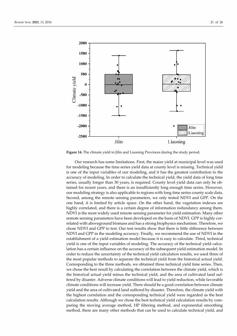
Remote Sens. 2021, 13, 2016 21 of 26

Figure 14. The climate yield in Jilin and Liaoning Provinces during the study period.

Our research has some limitations. First, the maize yield at municipal level was used

for modeling because the time series yield data at county level is missing. Technical yield

is one of the input variables of our modeling, and it has the greatest contribution to the

accuracy of modeling. In order to calculate the technical yield, the yield data of long time

series, usually longer than 30 years, is required. County level yield data can only be ob-

tained for recent years, and there is an insufficiently long enough time series. However,

our modeling strategy is also applicable to regions with long time series county scale data.

Second, among the remote sensing parameters, we only tested NDVI and GPP. On the

one hand, it is limited by article space. On the other hand, the vegetation indexes are

highly correlated, and there is a certain degree of information redundancy among them.

NDVI is the most widely used remote sensing parameter for yield estimation. Many other

remote sensing parameters have been developed on the basis of NDVI. GPP is highly cor-

related with aboveground biomass and has a strong biophysics mechanism. Therefore, we

chose NDVI and GPP to test. Our test results show that there is little difference between

NDVI and GPP in the modeling accuracy. Finally, we recommend the use of NDVI in the

establishment of a yield estimation model because it is easy to calculate. Third, technical

yield is one of the input variables of modeling. The accuracy of the technical yield calcu-

lation has a certain influence on the accuracy of the subsequent yield estimation model. In

order to reduce the uncertainty of the technical yield calculation results, we used three of

the most popular methods to separate the technical yield from the historical actual yield.

Corresponding to the three methods, we obtained three technical yield time series. Then,

we chose the best result by calculating the correlation between the climate yield, which is

the historical actual yield minus the technical yield, and the area of cultivated land suf-

fered by disaster. Adverse climate conditions will lead to yield reduction, while favorable

climate conditions will increase yield. There should be a good correlation between climate

yield and the area of cultivated land suffered by disaster. Therefore, the climate yield with

the highest correlation and the corresponding technical yield were regarded as the best

calculation results. Although we chose the best technical yield calculation results by com-

paring the moving average method, HP filtering method, and exponential smoothing

method, there are many other methods that can be used to calculate technical yield, and

Remote Sens. 2021, 13, 2016 22 of 26

these methods can be tested in the future. Fourth, the agrometeorological indexes and

remote sensing vegetation parameters used for model building in this study are monthly

scale data and calculated in a fixed time period (April to September). However, maize

phenology varies among different regions and require different climate conditions at dif-

ferent growth phases. Dividing the growth season of maize into multiple phases and cal-

culating agrometeorological indexes and remote sensing vegetation parameters for each

phase can better capture the impact of climate conditions of different growth phases on

maize yield. Fifth, a large quantity of remote sensing data, meteorological data, and sta-

tistical data with a long time series were used in this study. Collecting and preprocessing

these data consume a great amount of computer storage and computation time. At pre-

sent, some earth science data and analysis cloud computing platforms such as GEE pro-

vide a large number of high resolution remote sensing data, meteorological data, ad-

vanced computing functions, and flexible user interfaces. If the experimental process of

this study were transferred to the cloud computing platform, the time cost and computer

storage cost would be greatly reduced. Meanwhile, the applicability of this research

method in other study areas could be tested with highly efficiency because the model con-

structed in this study has explorability, simplicity, and convenience. Therefore, the wide

use of the cloud computing platforms for data calculation and processing is a new trend

which will assist greatly in yield estimation with big data processing.

6. Conclusions

In this paper, we combined technical yields, agrometeorological indexes, and remote

sensing vegetation parameters together to build maize yield estimation models for Liao-

ning and Jilin Provinces. We validated the accuracy of yield estimations models built in

this study, compared the differences of the two variable selection methods and discussed

the importance of different variables on yield estimation. The main conclusions are as fol-

lows:

First, the validation results show that the models built in this study have good appli-

cation potential and are suitable for both normal and disaster years. R2, CCC, and MARE

of yield estimation model built in Jilin Province were 0.8201,0.9761, and 0.0942, and they

were 0.7353, 0.8783 and 0.1128 in Liaoning Province, respectively. The average error of

yield estimation for the three disaster years was 0.12 in Jilin Province and 0.13 in Liaoning

Province.

Second, the accuracy of the two-stage importance evaluation method was better

than, or equivalent to, that of the other method, but it used the fewest variables. It is better

to group the variables according to their physical meaning, and to select important varia-

bles from each group, than to input all variables at one time and select important variables

to build the model.

Third, the contribution of the agrometeorological indexes to the improvement of the

overall modeling accuracy in the two provinces was greater than that of the remote sens-

ing parameters. The ATT variables were more important than the EDD variables. SPI2 in

July has a great impact on maize yield in both Jilin and Liaoning Provinces. GPPa (NDVIa)

in August is more important than the GPPa (NDVIa) variables in the other months.

Our study can not only be used as yield estimation tool for the related users, but also

guide the relevant researchers to establish similar yield estimation models in other re-

gions. In future, we can build such models using the cloud computing platform, which

will greatly reduce the time cost and computer storage cost.

Author Contributions: Conceptualization, X.Z.; Data curation, X.Z., R.G., T.L., and K.X.; Formal

analysis, R.G.; Funding acquisition, X.Z.; Investigation, R.G.; Methodology, X.Z.; Software, R.G.;

Validation, R.G.; Visualization, X.Z. and R.G.; Writing—original draft, X.Z.; Writing—review and

editing, X.Z., R.G., T.L., and K.X. All authors have read and agreed to the published version of the

manuscript.

Remote Sens. 2021, 13, 2016 23 of 26

Funding: This work was supported by the National Key R&D Program of China (Grant No.

2019YFA0606900) and the National Natural Science Foundation of China (Grant No. 42077436).

Data Availability Statement: Data is available upon request.

Acknowledgments: We thank the journal’s editors and reviewers for their kind comments and val-

uable suggestions to improve the quality of this paper.

Conflicts of Interest: The authors declare no conflict of interest.

References

1. Van Ittersum, M.K.; Cassman, K.G.; Grassini, P.; Wolf, J.; Tittonell, P.; Hochman, Z. Yield gap analysis with local to global

relevance–A review. Field Crop. Res. 2013, 143, 4–17, doi:10.1016/j.fcr.2012.09.009.

2. Lobell, D.B.; Cassman, K.G.; Field, C.B. Crop yield gaps: their importance, magnitudes, and causes. Annu. Rev. Environ. Resour.

2009, 34, 179–204, doi:10.1146/annurev.environ.041008.093740.

3. Murthy, C.S.; Thiruvengadachari, S.; Raji, P.V.; Jonna, S. Improved ground sampling and crop yield estimation using satellite

data. Int. J. Remote Sens. 1996, 17, 945–956, doi:10.1080/01431169608949057.

4. Kasampalis, D.A.; Alexandridis, T.K.; Deva, C.; Challinor, A.; Moshou, D.; Zalidis, G. Contribution of remote sensing on crop

models: A review. J. Imaging 2018, 4, 52, doi:10.3390/jimaging4040052.

5. Moulin, S.; Bondeau, A.; Delecolle, R. Combining agricultural crop models and satellite observations: From field to regional

scales. Int. J. Remote Sens. 1998, 19, 1021–1036, doi:10.1080/014311698215586.

6. Yao, F.; Tang, Y.; Wang, P.; Zhang, J. Estimation of maize yield by using a process-based model and remote sensing data in the

Northeast China Plain. Phys. Chem. Earth 2015, 87–88, 142–152, doi:10.1016/j.pce.2015.08.010.

7. Huang, J.; Sedano, F.; Huang, Y.; Ma, H.; Li, X.; Liang, S.; Tian, L.; Zhang, X.; Fan, J.; Wu, W. Assimilating a synthetic Kalman

filter leaf area index series into the WOFOST model to improve regional winter wheat yield estimation. Agric. For. Meteorol.

2016, 216, 188–202, doi:10.1016/j.agrformet.2015.10.013.

8. Shanahan, J.F.; Schepers, J.S.; Francis, D.D.; Varvel, G.E.; Wilhelm, W.W.; Tringe, J.M.; Schlemmer, M.R.; Major, D.J. Use of

remote-sensing imagery to estimate corn grain yield. Agron. J. 2001, 93, 583–589, doi:10.2134/agronj2001.933583x.

9. Panda, S.S.; Ames, D.P.; Panigrahi, S. Application of vegetation indices for agricultural crop yield prediction using neural

network techniques. Remote Sens. 2010, 2, 673–696, doi:10.3390/rs2030673.

10. Becker-Reshef, I.; Vermote, E.; Lindeman, M.; Justice, C. A generalized regression-based model for forecasting winter wheat

yields in Kansas and Ukraine using MODIS data. Remote Sens. Environ. 2010, 114, 1312–1323, doi:10.1016/j.rse.2010.01.010.

11. Palosuo, T.; Kersebaum, K.C.; Angulo, C.; Hlavinka, P.; Moriondo, M.; Olesen, J.E.; Patil, R.H.; Ruget, F.; Rumbaur, C.; Takac,

J.; et al. Simulation of winter wheat yield and its variability in different climates of Europe: A comparison of eight crop growth

models. Eur. J. Agron. 2011, 35, 103–114, doi:10.1016/j.eja.2011.05.001.

12. Eitzinger, J.; Thaler, S.; Schmid, E.; Strauss, F.; Ferrise, R.; Moriondo, M.; Bindi, M.; Palosuo, T.; Rotter, R.; Kersebaum, K.C.; et

al. Sensitivities of crop models to extreme weather conditions during flowering period demonstrated for maize and winter

wheat in Austria. J. Agric. Sci. 2013, 151, 813–835, doi:10.1017/s0021859612000779.

13. Asseng, S.; Ewert, F.; Martre, P.; Roetter, R.P.; Lobell, D.B.; Cammarano, D.; Kimball, B.A.; Ottman, M.J.; Wall, G.W.; White,

J.W.; et al. Rising temperatures reduce global wheat production. Nat. Clim. Chang. 2015, 5, 143–147, doi:10.1038/nclimate2470.

14. Barlow, K.M.; Christy, B.P.; O’Leary, G.J.; Riffkin, P.A.; Nuttall, J.G. Simulating the impact of extreme heat and frost events on

wheat crop production: A review. Field Crop. Res. 2015, 171, 109–119, doi:10.1016/j.fcr.2014.11.010.

15. Glotter, M.J.; Moyer, E.J.; Ruane, A.C.; Elliott, J.W. Evaluating the sensitivity of agricultural model performance to different

climate inputs. J. Appl. Meteorol. Climatol. 2016, 55, 579–594, doi:10.1175/jamc-d-15-0120.1.

16. Rotter, R.P.; Palosuo, T.; Kersebaum, K.C.; Angulo, C.; Bindi, M.; Ewert, F.; Ferrise, R.; Hlavinka, P.; Moriondo, M.; Nendel, C.;

et al. Simulation of spring barley yield in different climatic zones of Northern and Central Europe: A comparison of nine crop

models. Field Crop. Res. 2012, 133, 23–36, doi:10.1016/j.fcr.2012.03.016.

17. van der Velde, M.; Tubiello, F.N.; Vrieling, A.; Bouraoui, F. Impacts of extreme weather on wheat and maize in France:

Evaluating regional crop simulations against observed data. Clim. Chang. 2012, 113, 751–765, doi:10.1007/s10584-011-0368-2.

18. Mladenova, I.E.; Bolten, J.D.; Crow, W.T.; Anderson, M.C.; Hain, C.R.; Johnson, D.M.; Mueller, R. Intercomparison of soil

moisture, evaporative stress, and vegetation indices for estimating corn and soybean yields over the US. IEEE J. Sel. Top. Appl.

Earth Obs. Remote Sens. 2017, 10, 1328–1343, doi:10.1109/jstars.2016.2639338.

19. Sepaskhah, A.R.; Fahandezh-Saadi, S.; Zand-Parsa, S. Logistic model application for prediction of maize yield under water and

nitrogen management. Agric. Water Manag. 2011, 99, 51–57, doi:10.1016/j.agwat.2011.07.019.

20. Geetha, M.C.S.; Shanthi, I.E. Predicting the soil profile through modified regression by discretisation algorithm for the crop

yield in Trichy district, India. Int. J. Grid Util. Comput. 2018, 9, 235–242, doi:10.1504/ijguc.2018.10015147.

21. Tittonell, P.; Shepherd, K.D.; Vanlauwe, B.; Giller, K.E. Unravelling the effects of soil and crop management on maize

productivity in smallholder agricultural systems of western Kenya—An application of classification and regression tree analysis.

Agric. Ecosyst. Environ. 2008, 123, 137–150, doi:10.1016/j.agee.2007.05.005.

22. Bognar, P.; Kern, A.; Pasztor, S.; Lichtenberger, J.; Koronczay, D.; Ferencz, C. Yield estimation and forecasting for winter wheat

in Hungary using time series of MODIS data. Int. J. Remote Sens. 2017, 38, 3394–3414, doi:10.1080/01431161.2017.1295482.

Remote Sens. 2021, 13, 2016 24 of 26

23. Huang, J.; Wang, H.; Dai, Q.; Han, D. Analysis of NDVI Data for Crop Identification and Yield Estimation. IEEE J. Sel. Top. Appl.

Earth Obs. Remote Sens. 2014, 7, 4374–4384, doi:10.1109/jstars.2014.2334332.

24. Ren, J.; Chen, Z.; Zhou, Q.; Tang, H. Regional yield estimation for winter wheat with MODIS-NDVI data in Shandong, China.

Int. J. Appl. Earth Obs. Geoinf. 2008, 10, 403–413, doi:10.1016/j.jag.2007.11.003.

25. Zhang, P.; Anderson, B.; Tan, B.; Huang, D.; Myneni, R. Potential monitoring of crop production using a satellite-based Climate-

Variability Impact Index. Agric. For. Meteorol. 2005, 132, 344–358, doi:10.1016/j.agrformet.2005.09.004.

26. Son, N.T.; Chen, C.F.; Chen, C.R.; Chang, L.Y.; Duc, H.N.; Nguyen, L.D. Prediction of rice crop yield using MODIS EVI-LAI

data in the Mekong Delta, Vietnam. Int. J. Remote Sens. 2013, 34, 7275–7292, doi:10.1080/01431161.2013.818258.

27. Kouadio, L.; Duveiller, G.; Djaby, B.; El Jarroudi, M.; Defourny, P.; Tychon, B. Estimating regional wheat yield from the shape

of decreasing curves of green area index temporal profiles retrieved from MODIS data. Int. J. Appl. Earth Obs. Geoinf. 2012, 18,

111–118, doi:10.1016/j.jag.2012.01.009.

28. Domenikiotis, C.; Spiliotopoulos, M.; Tsiros, E.; Dalezios, N.R. Early cotton yield assessment by the use of the NOAA/AVHRR

derived Vegetation Condition Index (VCI) in Greece. Int. J. Remote Sens. 2004, 25, 2807–2819, doi:10.1080/01431160310001632729.

29. Salazar, L.; Kogan, F.; Roytman, L. Use of remote sensing data for estimation of winter wheat yield in the United States. Int. J.

Remote Sens. 2007, 28, 3795–3811, doi:10.1080/01431160601050395.

30. Meroni, M.; Marinho, E.; Sghaier, N.; Verstrate, M.M.; Leo, O. Remote sensing based yield estimation in a stochastic

framework—Case study of durum wheat in tunisia. Remote Sens. 2013, 5, 539–557, doi:10.3390/rs5020539.

31. Sakamoto, T.; Gitelson, A.A.; Arkebauer, T.J. MODIS-based corn grain yield estimation model incorporating crop phenology

information. Remote Sens. Environ. 2013, 131, 215–231, doi:10.1016/j.rse.2012.12.017.

32. Sakamoto, T.; Gitelson, A.A.; Arkebauer, T.J. Near real-time prediction of US corn yields based on time-series MODIS data.

Remote Sens. Environ. 2014, 147, 219–231, doi:10.1016/j.rse.2014.03.008.

33. Bala, S.K.; Islam, A.S. Correlation between potato yield and MODIS-derived vegetation indices. Int. J. Remote Sens. 2009, 30,

2491–2507, doi:10.1080/01431160802552744.

34. Seffrin, R.; de Araujo, E.C.; Bazzi, C.L. Regression models for prediction of corn yield in the state of Parana (Brazil) from 2012

to 2014. Acta Sci. Agron. 2018, 40, e36494, doi:10.4025/actasciagron.v40i1.36494.

35. Mathieu, J.A.; Aires, F. Assessment of the agro-climatic indices to improve crop yield forecasting. Agric. For. Meteorol. 2018, 253,

15–30, doi:10.1016/j.agrformet.2018.01.031.

36. Holzman, M.E.; Carmona, F.; Rivas, R.; Niclos, R. Early assessment of crop yield from remotely sensed water stress and solar

radiation data. ISPRS J. Photogramm. Remote Sens. 2018, 145, 297–308, doi:10.1016/j.isprsjprs.2018.03.014.

37. Zhang, J.Q. Risk assessment of drought disaster in the maize-growing region of Songliao Plain, China. Agric. Ecosyst. Environ.

2004, 102, 133–153, doi:10.1016/j.agee.2003.08.003.

38. Ming, B.; Guo, Y.; Tao, H.; Liu, G.; Li, S.; Wang, P. SPEIPM-based research on drought impact on maize yield in North China

Plain. J. Integr. Agric. 2015, 14, 660–669, doi:10.1016/s2095-3119(14)60778-4.

39. Xu, X.; Gao, P.; Zhu, X.; Guo, W.; Ding, J.; Li, C. Estimating the responses of winter wheat yields to moisture variations in the

past 35 years in Jiangsu Province of China. PLoS ONE 2018, 13, e0191217, doi:10.1371/journal.pone.0191217.

40. Wang, S.; Mo, X.; Hu, S.; Liu, S.; Liu, Z. Assessment of droughts and wheat yield loss on the North China Plain with an aggregate

drought index (ADI) approach. Ecol. Indic. 2018, 87, 107–116, doi:10.1016/j.ecolind.2017.12.047.

41. Chen, F.; Jia, H.; Pan, D. Risk assessment of maize drought in china based on physical vulnerability. J. Food Qual. 2019, 2019,

9392769, doi:10.1155/2019/9392769.

42. Lalic, B.; Eitzinger, J.; Thaler, S.; Vucetic, V.; Nejedlik, P.; Eckersten, H.; Jacimovic, G.; Nikolic-Djoric, E. can agrometeorological

indices of adverse weather conditions help to improve yield prediction by crop models? Atmosphere 2014, 5, 1020–1041,

doi:10.3390/atmos5041020.

43. Shumin, L. Comprehensive evaluation on the drought risk of rain-fed agriculture in China based on GIS. J. Arid Land Resour.

Environ. 2011, 25, 39–44, doi:10.1016/B978-0-444-53599-3.10005-8.

44. Chavas, D.R.; Izaurralde, R.C.; Thomson, A.M.; Gao, X. Long-term climate change impacts on agricultural productivity in

eastern China. Agric. For. Meteorol. 2009, 149, 1118–1128, doi:10.1016/j.agrformet.2009.02.001.

45. Zhou, B.; Xu, Y.; Wu, J.; Dong, S.; Shi, Y. Changes in temperature and precipitation extreme indices over China: Analysis of a

high-resolution grid dataset. Int. J. Climatol. 2016, 36, 1051–1066, doi:10.1002/joc.4400.

46. Wu, H.; Hou, W.; Qian, Z.-H.; Hu, J.-G. The research on the sensitivity of climate change in China in recent 50 years based on

composite index. Acta Phys. Sin. 2012, 61, 149205, doi:10.7498/aps.61.149205.

47. Gao, G.; Huang, C.Y. Climate change and its impact on water resources in North China. Adv. Atmos. Sci. 2001, 18, 718–732,

doi:10.1142/S0252959901000401.

48. Hersbach, H.; Bell, B.; Berrisford, P.; Hirahara, S.; Horányi, A.; Muñoz-Sabater, J.; Nicolas, J.; Peubey, C.; Radu, R.; Schepers, D.;

et al. The ERA5 global reanalysis. Q. J. R. Meteorol. Soc. 2020, 146, 1999–2049, doi:10.1002/qj.3803.

49. National Earth System Science Data Center. National Science & Technology Infrastructure of China. Availabe online:

http://www.geodata.cn/ (accessed on 7 June 2020).

50. Yuan, W.; Liu, S.; Yu, G.; Bonnefond, J.M.; Chen, J.; Davis, K.; Desai, A.R.; Goldstein, A.H.; Gianelle, D.; Rossi, F. Global estimates

of evapotranspiration and gross primary production based on MODIS and global meteorology data. Remote Sens. Environ. 2010,

114, 1416–1431, doi:10.1016/j.rse.2010.01.022.

Remote Sens. 2021, 13, 2016 25 of 26

51. Land Long Term Data Record. Available online: https://ltdr.modaps.eosdis.nasa.gov/cgi-bin/ltdr/ltdrPage.cgi (accessed on 8

June 2020).

52. Gooijer, J.G.D.; Hyndman, R.J. 25 years of time series forecasting. Monash Econom. Bus. Stats Work. Pap. 2005, 22, 443–473,

doi:10.2139/ssrn.748904.

53. Ravn, M.O.; Uhlig, H. On Adjusting the Hodrick-Prescott filter for the frequency of observations. Rev. Econ. Stats 2002, 84, 371–

375, doi:10.1162/003465302317411604.

54. Gardner, E.S. Forecasting the failure of component parts in computer systems: A case study. Int. J. Forecast. 1993, 9, 245–253,

doi:10.1016/0169-2070(93)90008-B.

55. Dong, W.; Liu, S.; Fang, Z. On modeling mechanisms and applicable ranges of grey incidence analysis models. Grey Syst. Theory

Appl. 2018, 8, 448–461, doi:10.1108/GS-04-2018-0019.

56. Junfu, X.; Zhandong, L.I.U.; Yumin, C. Study on the water requirement and water requirement regulation of maize in china.

Maize Sci. 2008, 16, 21–25.

57. Cao, X.; Wang, Y.; Wu, P.; Zhao, X.; Wang, J. An evaluation of the water utilization and grain production of irrigated and rain-

fed croplands in China. Sci. Total Environ. 2015, 529, 10–20, doi:10.1016/j.scitotenv.2015.05.050.

58. Sun, F.; Yang, X.; Lin, E.; Ju, H.; Xiong, W. Study on the sensitivity and vulnerability of wheat to climate change in china. Sci.

Agric. Sin. 2005, 38, 692–696.

59. Wang, J.; Yang, X.; Lu, S.; Liu, Z.; Li, K.; Xun, X.; Liu, Y.; Wang, E. Spatial-temporal characteristics of potential yields and yield

gaps of spring maize in Heilongjiang province. Sci. Agric. Sin. 2012, 45, 1914–1925, doi:10.3864/j.issn.0578-1752.2012.10.004.

60. Leng, G.Y.; Hall, J. Crop yield sensitivity of global major agricultural countries to droughts and the projected changes in the

future. Sci. Total Environ. 2019, 654, 811–821, doi:10.1016/j.scitotenv.2018.10.434.

61. Yu, X.; He, X.; Zheng, H.; Guo, R.; Ren, Z.; Zhang, D.; Lin, J. Spatial and temporal analysis of drought risk during the crop-

growing season over northeast China. Nat. Hazards 2014, 71, 275–289, doi:10.1007/s11069-013-0909-2.

62. Zhang, Z.; Chen, Y.; Wang, P.; Zhang, S.; Tao, F.; Liu, X. Spatial and temporal changes of agro-meteorological disasters affecting

maize production in China since 1990. Nat. Hazards 2014, 71, 2087–2100, doi:10.1007/s11069-013-0998-y.

63. McKee, T.B.; Doesken, N.J.; Kleist, J. The relationship of drought frequency and duration of time scales. In Proceedings of the

Eight Conference on Apllied Climatology, American Meteorological Society, Anaheim, CA, USA, 17–23 January 1993; pp. 179–

186.

64. Sanchez, B.; Rasmussen, A.; Porter, J.R. Temperatures and the growth and development of maize and rice: A review. Glob. Chang.

Biol. 2014, 20, 408–417, doi:10.1111/gcb.12389.

65. Hawkins, E.; Fricker, T.E.; Challinor, A.J.; Ferro, C.A.T.; Ho, C.K.; Osborne, T.M. Increasing influence of heat stress on French

maize yields from the 1960s to the 2030s. Glob. Chang. Biol. 2013, 19, 937–947, doi:10.1111/gcb.12069.

66. Lobell, D.B.; Hammer, G.L.; McLean, G.; Messina, C.; Roberts, M.J.; Schlenker, W. The critical role of extreme heat for maize

production in the United States. Nat. Clim. Chang. 2013, 3, 497–501, doi:10.1038/nclimate1832.

67. Lobell, D.B.; Sibley, A.; Ivan Ortiz-Monasterio, J. Extreme heat effects on wheat senescence in India. Nat. Clim. Chang. 2012, 2,

186–189, doi:10.1038/nclimate1356.

68. Schlenker, W.; Roberts, M.J. Nonlinear temperature effects indicate severe damages to US crop yields under climate change.

Proc. Natl. Acad. Sci. USA 2009, 106, 15594–15598, doi:10.1073/pnas.0906865106.

69. Chen, J.; Jonsson, P.; Tamura, M.; Gu, Z.H.; Matsushita, B.; Eklundh, L. A simple method for reconstructing a high-quality NDVI

time-series data set based on the Savitzky-Golay filter. Remote Sens. Environ. 2004, 91, 332–344, doi:10.1016/j.rse.2004.03.014.

70. Papagiannopoulou, C.; Miralles, D.G.; Decubber, S.; Demuzere, M.; Verhoest, N.E.C.; Dorigo, W.A.; Waegeman, W. A non-

linear Granger-causality framework to investigate climate-vegetation dynamics. Geosci. Model. Dev. 2017, 10, 1945–1960,

doi:10.5194/gmd-10-1945-2017.

71. Schaefer, K.; Schwalm, C.R.; Williams, C.; Arain, M.A.; Barr, A.; Chen, J.M.; Davis, K.J.; Dimitrov, D.; Hilton, T.W.; Hollinger,

D.Y.; et al. A model-data comparison of gross primary productivity: Results from the North American Carbon Program site

synthesis. J. Geophys. Res. Biogeosci. 2012, 117, 15, doi:10.1029/2012jg001960.

72. Wang, Y.; Tang, P.; Li, S.; Tian, Y.; Li, J. The water demand and optimal irrigation schedule of maize in drought years at eastern

area of Inner Mongolia. Agric. Res. Arid Areas 2018, 36, 108–114.

73. Gao, X.; Wang, C.; Zhang, J.; Xue, X. Crop water requirement and temporal-spatial variation of drought and flood disaster

during growth stages for maize in Northeast during past 50 years. Trans. Chin. Soc. Agric. Eng. 2012, 28, 101–109.

74. Cao, Y.; Yu, Z.; Zhao, T. Study of water demand and consumption rules in summer maize. Acta Agric. Boreali-Sin. 2003, 18, 47–

50.

75. Song, L.; Jin, J.; He, J. Effects of Severe Water Stress on Maize Growth Processes in the Field. Sustainability 2019, 11, 5086,

doi:10.3390/su11185086.

76. Aktas, A.F.; Ustundag, B.B. Phenology Based NDVI Time-series Compensation for Yield Estimation Analysis. In Proceedings

of the 6th International Conference on Agro-Geoinformatics, Fairfax, VA, USA, 7–10 August 2017; pp. 1–5.

77. Govedarica, M.; Jovanovic, D.; Sabo, F.; Borisov, M.; Vrtunski, M.; Alargic, I. Comparison of MODIS 250 m products for early

corn yield predictions: A case study in Vojvodina, Serbia. Open Geosci. 2016, 8, 747–759, doi:10.1515/geo-2016-0070.

78. Moriondo, M.; Maselli, F.; Bindi, M. A simple model of regional wheat yield based on NDVI data. Eur. J. Agron. 2007, 26, 266–

274, doi:10.1016/j.eja.2006.10.007.

Remote Sens. 2021, 13, 2016 26 of 26

79. Mkhabela, M.S.; Mkhabela, M.S.; Mashinini, N.N. Early maize yield forecasting in the four agro-ecological regions of Swaziland

using NDVI data derived from NOAAs-AVHRR. Agric. For. Meteorol. 2005, 129, 1–9, doi:10.1016/j.agrformet.2004.12.006.

80. Liu, J.; He, X.; Wang, P.; Huang, J. Early prediction of winter wheat yield with long time series meteorological data and random

forest method. Trans. Chin. Soc. Agric. Eng. 2019, 35, 158–166, doi:10.11975/j.issn.1002-6819.2019.06.019.

81. Mutanga, O.; Adam, E.; Cho, M.A. High density biomass estimation for wetland vegetation using WorldView-2 imagery and

random forest regression algorithm. Int. J. Appl. Earth Obs. Geoinf. 2012, 18, 399–406, doi:10.1016/j.jag.2012.03.012.

82. Cai, Y.; Guan, K.; Lobell, D.; Potgieter, A.B.; Wang, S.; Peng, J.; Xu, T.; Asseng, S.; Zhang, Y.; You, L., et al. Integrating satellite

and climate data to predict wheat yield in Australia using machine learning approaches. Agric. For. Meteorol. 2019, 274, 144–159,

doi:10.1016/j.agrformet.2019.03.010.

83. Huang, J.; Ma, H.; Liu, J.; Zhu, D.; Zhang, X. Regional winter wheat yield estimation by assimilating MODIS ET and LAI

products into SWAP model. In Second International Conference on Agro-Geoinformatics, Fairfax, VA, USA, 12–16 August 2013;

pp. 452–457.

84. Feng, P.; Wang, B.; Liu, D.L.; Waters, C.; Yu, Q. Incorporating machine learning with biophysical model can improve the

evaluation of climate extremes impacts on wheat yield in south-eastern Australia. Agric. For. Meteorol. 2019, 275, 100–113,

doi:10.1016/j.agrformet.2019.05.018.