Crop model- and satellite imagery-basedrecommendation tool for variable rate N fertilizerapplication for the US Corn system

Zhenong Jin1,2 • Rishi Prasad3 • John Shriver3 •

Qianlai Zhuang1,4

� Springer Science+Business Media New York 2016

Abstract Precision nitrogen (N) management for corn has gained popularity due to both

economic and environmental considerations. There is sufficient evidence demonstrating

that N fertilizer efficiency can be improved by implementing sidedress and variable rate

fertilization. In this paper, a crop model- and satellite imagery-based decision-support tool

for recommending variable rate N fertilization at a high resolution of 5 m 9 5 m is

introduced. The sub-field management zones were delineated by overlapping the soil

survey geographic (SSURGO) soil map units with wide dynamic range vegetation index

(WDRVI)-derived relative productivity zones. The calibrated Agricultural Production

Systems sIMulator (APSIM) was used to simulate a range of soil N processes, corn growth

and N uptake by assimilating real-time weather data from the National Climate Data

Center (NCDC). Sidedress N rates were estimated based on the target rate, N loss via

leaching and denitrification, plant uptake and leftover N in the soil. The tool was tested on

a 66 ha corn field in Illinois, USA for the growing season of 2015. Results showed that

N-Prescription was able to give reasonable management zone delineation and sidedress N

recommendation. The recommended sidedress N ranged from 60 to over 120 kg ha-1.

Corn yield was greater in areas with higher sidedress recommendation, but the benefit from

sidedress decreased with the increasing rate and plateaued above 110 kg ha-1. Sensitivity

analysis suggested that soil hydraulic properties and soil organic matter content were

Electronic supplementary material The online version of this article (doi:10.1007/s11119-016-9488-z)contains supplementary material, which is available to authorized users.

& Qianlai Zhuangqzhuang@purdue.edu

1 Department of Earth, Atmospheric and Planetary Science, Purdue University, CIVIL 550 StadiumMall Drive, West Lafayette, IN 47907-2051, USA

2 Department of Earth System Science and Center on Food Security and the Environment, StanfordUniversity, Stanford, CA 94305, USA

3 Farmlogs, Ann Arbor, MI 48104, USA

4 Department of Agronomy, Purdue University, West Lafayette, IN 47907, USA

123

Precision AgricDOI 10.1007/s11119-016-9488-z

critical to the sidedress accounting. Corn growth, and hence the cumulative N uptake, can

be well simulated by calibrating the WDRVI derived leaf area index. This tool could serve

as a good foundation for further development in precision N management.

Keywords Precision fertilization � Sidedress � Corn � Agricultural Production Systems

sIMulator (APSIM) � Wide dynamic range vegetation index (WDRVI) � SSURGO

Introduction

Nitrogen (N) is one of the primary limiting factors for corn (Zea mays L.) yield and quality

(Scharf 2015). Corn with deficient N will have dwarfed seedlings and yellowish leaves,

leading to partial or complete failure of kernel setting (Ma and Biswas 2015). While

adequate N is necessary for proper plant development and optimal grain yield, over-

fertilizing risks contamination of water at local and regional scales (Keeney and Olson

1986; McIsaac et al. 2002), and nitrous oxide (a potent greenhouse gas) emissions (Park

et al. 2012; Scharf 2015). The need to wisely manage N fertilizer is thus compelling for

both economic and environmental considerations (Scharf 2015).

In practice, the producer-level associated cost of under-fertilization relative to over-

fertilization drives farmers to apply N at greater rates, as additional ‘‘insurance’’ against

yield losses (Moebius-Clune et al. 2013). It is estimated that 75% of N fertilizer for the US

Corn-Belt (typically covering Iowa, Illinois, Indiana, southern Michigan, western Ohio,

eastern Nebraska, eastern Kansas, southern Minnesota and parts of Missouri) is applied

before planting (Cassman et al. 2002), among which fall application is more widely

practiced than spring application. The N fertilizer loss is highly weather dependent, and is

greatest in warm and wet winters (Randall et al. 2003; Tremblay et al. 2012; Scharf 2015).

Thus, to reduce N losses before the growing season begins, a good strategy is to apply a

portion of N in-season (Thompson et al. 2015). Furthermore, applying N based on soil

heterogeneity can reduce the overall N rate applied and increase profitability compared

with a uniform N application (Mamo et al. 2003).

The optimal management of N requires a farmer to make a series of decisions on the

form (what), timing (when), placement (where) and rate (how much) of N fertilizer to be

applied. While the N form and timing is often limited by accessibility and logistic con-

straints, determining where and how much N fertilizer should be applied is more science-

oriented (Scharf 2015), and has progressed considerably in recent years (Setiyono et al.

2011; Shahandeh et al. 2011; Solie et al. 2012; Moebius-Clune et al. 2013; Thompson et al.

2015). It is well established that the optimal N rate for a given field depends on crop

demands, indigenous N supply as a net result of mineralization and immobilization, and

losses of N fertilizer or soil-derived N via leaching, denitrification and volatilization. Each

of these aforementioned processes interacts among themselves, and is influenced by many

factors such as seasonal temperature, precipitation, soil physical and biogeochemical

properties, and management history. Although researchers have spent considerable efforts

to understand the complexity associated with N management, the uncertainty is still

substantial (Scharf 2015). The problem is further complicated by spatial variations in soil

N contribution, fertilizer losses and crop N uptake from field to field and even place to

place within a field. N mineralization of SOM may vary because of differences in organic

N release rate as a function of soil temperature and moisture, or differences in past crop

removal (Scharf 2015). N leaching loss can vary mainly because of different topography

and soil hydrological properties (Prasad et al. 2015). The N fertilizer needed by the crop

Precision Agric

123

can vary as a result of varying yield potential (Mamo et al. 2003), or differences in seeding

rates. Because of these complexities, a fast and accurate diagnostic tool for the optimal N

rate for a given field remains a challenge (Ma and Biswas 2015; Scharf 2015).

Crop models that simulate all the aforementioned N processes have been identified as a

management tool for synchronizing N fertilizer application with crop N demand (Cassman

et al. 2002; Scharf 2015). A number of specific simulation models have been developed to

optimize pre-plant or in-season N management from either public research institutes or

private sectors, among which Adapt-N (Melkonian et al. 2008; Moebius-Clune et al. 2013;

Sela et al. 2016) and Maize-N (Setiyono et al. 2011; Thompson et al. 2015) are two such

examples that are still in active development. The Maize-N tool is built on the Hybrid-

Maize model (Yang et al. 2006), and estimates the N sidedress based on a spherical

function that relates yield to N rate (Setiyono et al. 2011). Maize-N in general recommends

substantially more N than sensor-based, in-season N recommendations, but was better at

protecting yield (Thompson et al. 2015). The Adapt-N model is built on the Precision

Nitrogen Management model (Melkonian et al. 2008), which consists of two major

components: (i) a corn growth model adapted from Sinclair and Muchow (1995), and (ii) a

biogeochemistry model that simulates water and solute transport (Sela et al. 2016), as well

as biochemical transformation of N. Adapt-N calculates N recommendation based on a

mass balance approach according to a number of factors, including the required N to

achieve the expected yield, N content in crop and soil, N credit from soybean rotation, and

a probabilistic estimation of future N gains minus losses (Sela et al. 2016). However,

neither Adapt-N nor Maize-N has been tested in terms of their capability to give variable

rate N within a field. Also, their operational use often requires the user to input a range of

field measurement data, lowering the potential of farmer use at scale.

The recent advent of high-performance computers and communication technologies has

made it possible to process massive remotely-sensed or field survey data and weather data in

near real-time to inform precision N management. Here for the first time, this study inves-

tigates the potential of very-high-resolution (5 m 9 5 m) on-farm N management by inte-

grating recent advances in a range of research areas, including remote sensing, cropmodeling

and soil mapping. The proposed tool uses remotely-sensed data to delineate within-field

management zones, simulates sub-field variations in soil and crop status with a crop model

that assimilates in situ soil database and real-time weather information, and finally delivers

either pre-plant or in-season variable rate N recommendations to match fertilizer application

with crop demand. The core part of a process-based crop model for estimating indigenous N

supply, N losses and crop N demand is built on the Agricultural Production Systems

sIMulator (APSIM) platform (Holzworth et al. 2014). In the following sections, detailed

science and engineering background of the N recommendation tool will be described, and a

case study for a typical USMidwest Corn field in Illinois, USA,will be presented. The goal of

this paper is to introduce a prototype and discuss possible improvements, with a hope that this

study will inspire others to investigate further on precision N management.

Materials and methods

Overview of workflow

The N-Prescription infrastructure is built on the Amazon Elastic Compute Cloud (EC2;

https://aws.amazon.com/ec2/), and has been parallelized to support multiple simulations at

Precision Agric

123

the same time. Amazon EC2 is a web service that provides resizable compute capacity in

the cloud. It is designed to make web-scale cloud computing easier for developers/pro-

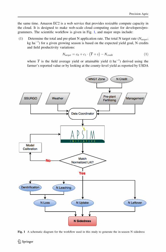
grammers. The scientific workflow is given in Fig. 1, and major steps include:

(1) Determine the total and pre-plant N application rate. The total N target rate (Ntarget;

kg ha-1) for a given growing season is based on the expected yield goal, N credits

and field productivity variations:

Ntarget ¼ c0 þ c1 � Y þ e� �

� Ncredit ð1Þ

where Y is the field average yield or attainable yield (t ha-1) derived using the

farmer’s reported value or by looking at the county-level yield as reported by USDA

Fig. 1 A schematic diagram for the workflow used in this study to generate the in-season N sidedress

Precision Agric

123

National Agricultural Statistics Service (NASS); e is the adjustment term that

accounts for spatial variability of long-term average soil fertility among productivity

zones and can be estimated by looking into the historical yield map generated by

harvest combine or derived from the multi-year averaged remote sensing images

(see section ‘‘The estimation of e and expected yield’’ for detailed discussion); Y þ eis thus the expected yield from each productivity zone; c0 and c1 is the offset and

slope for calculating state-specific N fertilizer requirement per unit yield (Table S1),

respectively; Ncredit is the credits for soil organic N from previous legume crops or

manure application (Table S2). Among the Ntarget, 50% is assumed to be applied

before planting as either fall or spring application.

(2) Data query. This step essentially collects all data required and creates simulation

files for the APSIM. It starts with importing a 5 m 9 5 m raster, clipped to the field

boundary. Based on the raster extent, soil parameters such as layered soil hydraulic

properties, soil pH and soil organic matter (SOM) are queried from the Soil Survey

Geographic (SSURGO) database (Soil Survey Staff 2015) and resampled to finer

vertical layers with depth 0–0.1, 0.1–0.2, 0.2–0.5, 0.5–1.0 and 1.0–2.0 m. When

there are multiple soil components within a grid, the largest fraction will be selected.

Detailed descriptions for soil parameters required for the model are presented in

Archontoulis et al. (2014). These parameters can be further refined once onsite soil

sampling data is available. Real time weather data for the site, including daily

maximum and minimum temperature, precipitation and solar radiation are from the

National Climate Data Center (NCDC), Asheville, NC, USA. Field management

information including sowing date, seeding rate and cultivar relative maturity is

input by users if available; otherwise, estimated values according to satellite

imagery and NASS report are assigned.

(3) Crop model simulation. The APSIM is run at a daily time step to provide soil and

crop N status, such as N leaching and denitrification, N leftover in soil and plant N

uptake. Instead of running the model for the whole field, the tool run the model for

virtual grids first, and then re-project outputs to the 5 m-resolution raster shapefile

according to a geographic reference table. A virtual grid is a unique combination of

soil type, seeding rates and management zone. For example, if there are 5 different

soil types, four levels of seeding rates and five productivity zones for a given field,

the number of virtual grids is 100. Using virtual grids substantially lowers the

computational cost. When observational data such as satellite or UAV imagery is

available, the crop model will be calibrated iteratively to match spectral-derived

vegetation indices (e.g. LAI).

(4) Calculating sidedress N rate. The sidedress N fertilizer rate (Nsidedress) is computed

using the equation:

Nsidedress ¼ Ntarget þ Nloss � Nuptake � Nleftover ð2Þ

where Nloss is the total N losses via denitrification (Ndenit) and leaching (Nleach) up-

to-date, Nuptake is the cumulative plant N uptake when sidedress N recommendation

is requested, and Nleftover is the remaining inorganic N up-to-date. The timing of

sidedress N application is assumed to be around V6 stage (Abendroth 2011), after

which rapid crop N uptake will happen. The N loss after sidedress is not explicitly

accounted for in the current framework, since both denitrification and leaching

during the remaining growing season are highly weather dependent and difficult to

Precision Agric

123

forecast. The N loss after sidedress application is assumed to be partly compensated

by gains of N via net mineralization of soil organic matter.

Management zone delineation

Management zone refers to the relatively homogeneous sub-units of a field, within which a

uniform management practice can be applied (Mulla 2013). Several approaches have been

developed to delineate site-specific management zones, such as based on soil character-

istics (Fleming et al. 2004), yield maps from multiple years (Diker et al. 2004), remotely

sensed spectral information (Zhang et al. 2010; Cicore et al. 2016), or more often based on

a combination of multiple data (Song et al. 2009; Shaddad et al. 2016). These layers of

information can be processed by various clustering algorithms to generate the management

zones, among which Fuzzy-k mean is so far the most popular option (Guastaferro et al.

2010). In this study, the management zones are delineated by combining the satellite

observed multi-year crop productivity and the soil types derived from SSURGO.

For a given field, the delineation starts with identifying the sub-field relative produc-

tivity zones based on the wide dynamic range vegetation index (WDRVI) derived from

RapidEye images. The RapidEye system is a constellation of five satellites that produces

multispectral images at a spatial resolution of 5 m 9 5 m; detailed description of radio-

metric and geometric properties of the RapidEye sensor is given in Chander et al. (2013).

The red (630–685 nm) and near infrared red (NIR) (760–850 nm) bands are used to

calculate the WDRVI following Gitelson (2004):

WDRVI ¼ aqNIR � qredaqNIR þ qred

ð3Þ

where q is the reflectance and a is a weighting coefficient set to be 0.2. Main steps to

classify the relative productivity zones include:

(1) Collect all WDRVI images between July 15th and September 1st for years

2009–2014 that are at least 90% cloud free. The time window from middle July to

early September is selected because previous studies showed that remotely sensed

vegetation indices during this period are most indicative for the final corn yield

(Sibley et al. 2014; Lobell et al. 2015). The Landsat-7 cloud filtering algorithm

(Irish, 2000) for automatic cloud cover assessment is applied to the radiometric data

in the Rapideye dataset, adjusting the thresholds based on a training dataset

collected over 50 images in the Midwestern US between 2009 and 2014.

(2) Apply L1 normalization to the WDRVI data (i.e. for each image, subtract the

minimum and then divide by the maximum). Pixels within 15 m of the field edge

were excluded, as field edges tend to show lower yields and WDRVI, but are too

narrow and costly to manage as separate zones.

(3) Average all the images within a year to generate a single image per year.

(4) Pass all the normalized annual mean images (one per year when data are available)

to an unsupervised k-means algorithm (Arthur and Vassilvitskii 2007) for

classification. The k-means algorithm, implemented in the ‘‘scikit-learn’’ package

for Python, divides the image pixels (x) into k clusters, by iteratively optimizing the

choice of cluster specific centroids (c) that can minimize the total within-cluster

distance between individual pixels and the corresponding centroid:

Precision Agric

123

Dtotal ¼Xk

j¼1

Xnj

i¼1

jjx jð Þi � cjjj ð4Þ

where xjð Þ

i is the ith pixel in jth cluster, and nj is the number of pixels classified into

the jth cluster. The gap statistic (Tibshirani et al. 2001) is used to estimate the

number of clusters (i.e. k) present in the dataset. The resulting clusters are labeled as

different productivity zones. These productivity zones will then be overlaid with the

SSURGO map units, and each unique combination of productivity zone and soil

map unit is treated as a separate management zone (Fig. S1).

Description of the APSIM

The APSIM is an agricultural system model that can simulate the growth of a number of

crops under various climatic, edaphic and management conditions (Holzworth et al. 2014).

In this study, the maize module in APSIM version 7.7 was used to model the phenology,

morphology, and biomass production for corn. The phenological phase progress was

simulated using the thermal time method (Wilson et al. 1995), and the radiation use

efficiency (RUE) based biomass production and partition was limited by temperature,

water and N stress (Hammer et al. 2009). The APSIM has recently been widely applied in

the US Corn-Belt to address a range of research questions related to the corn production

and cropping system management (Hammer et al. 2009; Lobell et al. 2013; Archontoulis

et al. 2014; Jin et al. 2016).

The SoilN module simulates the dynamics of soil carbon (C) and N on a daily basis,

with N mineralization, immobilization, nitrification, denitrification and urea hydrolysis

explicitly described in each soil layer. The layer-specific SOM is divided into a fast

decomposing pool (BIOM) and a less active pool (HUM). To account for the age of

different organic residuals, part of the HUM pool is further specified as a recalcitrant pool

(INERT), with the fraction to be larger in deeper soil layers. Organic N sequestrated by

SOM will be gradually released through mineralization according to the decomposing of

each soil C pools, with the rate mediated by soil temperature, moisture and C/N ratio. More

fresh organic matter is stored in a separate pool (FOM), and is initialized by root weight

and root C/N ratio. The FOM pool contains three sub-pools, namely the carbohydrate-like,

cellulose-like and lignin-like pools, with default fractions set as 0.2, 0.7 and 0.1, respec-

tively. The APSIM also supports manure application through the SurfaceOM module,

which describes the organic N fractions in the same way as the FOM pool. When N

fertilizer is applied, the N will enter the inorganic N pools of Urea-N, NH4-N and NO3-N,

with the fraction determined by the fertilizer type.

These soil N processes are primarily controlled by soil temperature, moisture, pH and

water flow through the soil profile. Daily soil temperature for each soil layer is simulated

by the SoilTemp module. Soil hydrology is simulated by the SoilWat module that uses a

cascading water balance model approach (Littleboy et al. 1992). This daily time-step

hydrology model includes: surface runoff (estimated via the USDA curve number method),

soil evaporation (estimated via the two-stage evaporation method), plant transpiration

(estimated via the transpiration efficiency approach), and vertical water flows and fluxes

that can transport N in soil solute through the soil profile. Parameters for these soil modules

are mainly derived from the SSURGO database, and a few are obtained through

calibration.

Precision Agric

123

SSURGO database

The SSURGO database is a compilation of county soil surveys by the USDA Natural

Resources Conservation Service (NRCS), and is typically available for most of the US

territories at a scale of 1:24 000. The SSURGO uses georeferenced map units to depict the

spatial distribution of soil components. Within each map unit, the fraction of the com-

ponent soils and their layer-specific properties are explicitly given. In this study, soil

information from SSURGO is queried using the R soilDB package that can interact with

the NRCS soil data access (SDA) web service. More details about the implementation of

soilDB are available at: http://ncss-tech.github.io/AQP/soilDB/SDA-tutorial.html (last

accessed 31 October 2016).

Although the only available option for widespread soil information in the focus region

of this paper, SSURGO has been questioned for not accurately representing the actual field

variability (Ashtekar and Owens 2013). In application, part of the required soil parameters,

such as soil texture and soil organic matter content, may be further tuned when onsite soil

sampling is available. Yet in the APSIM, the simulation of soil N and hydrological pro-

cesses are controlled by more than one hundred parameters. What are the most important

parameters to measure remains an open question. As a starting point, a global sensitivity

analysis (GSA) was conducted following Pappas et al. (2013) to identify the most sensitive

soil parameters for N uptake, denitrification, leaching and net N mineralization. Detailed

implementations of the GSA are presented in the Supplementary Material (Text S1), and

candidate parameters along with their initial values are listed in Table S3.

Model calibration

Traditional model calibration for a specific location requires a range of field measurement

and is very labor-intensive (Archontoulis et al. 2014), and thus is not suitable for devel-

oping a computationally efficient and spatially extensible N management tool. In this

prototype, model calibration mainly focuses on matching the early season LAI. In the

APSIM, LAI directly controls the canopy intercepted solar radiation, which limits the

biomass production, and the accumulated biomass will in turn be allocated to build LAI.

Because of this feedback, any bias in LAI simulation (especially in early seasons between

emergence and V5/V6 stages) will lead to unreasonable simulation of corn growth and N

uptake. On the other hand, APSIM by default tends to substantially underestimate the early

season LAI, and hence crop N uptake. Therefore, the current calibration was primarily for

correcting the systematic underestimation of LAI in the early season.

Ideally this should be done by calibrating the APSIM LAI simulation against a series of

observed spectral information of the current growing season up to the date when N sid-

edressing is calculated. However, cloud-free satellite images are often too limited for the

period between crop emergence and V5/V6 stages to give sufficient degrees of freedom for

observations. One feasible solution is to use UAV images that can be obtained with higher

temporal frequency, which is out of the scope of this study (the pros and cons of this

solution will be discussed later). Alternatively, when high quality WDRVI images are

sufficient for the previous year, it is feasible to derive parameters by calibrating the model

using WDRVI values of the previous year. The two underpinning assumptions are: (i) the

cultivar grown in the same field is similar between two years, and (ii) calibration for the

whole season LAI curve helps to reduce the underestimation in early season. Here, two

methods for LAI calibration were introduced. The first method (named Calibration-1

Precision Agric

123

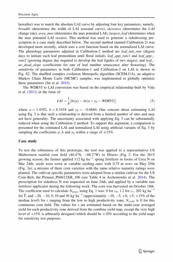
hereafter) was to match the absolute LAI curve by adjusting four key parameters, namely,

breadth (determines the width of LAI seasonal curve), skewness (determines the LAI

change rate), area_max (determines the max potential LAI), largest_leaf (determines when

the max potential LAI occurs). This method was used to generate a sidedressing pre-

scription in a case study described below. The second method (named Calibration-2) was

developed more recently, which uses a cost function based on the normalized LAI curve.

The phenology parameters adjusted in Calibration-2 method are leaf_init_rate (degree

days to initiate each leaf primordium until floral initial), leaf_app_rate1 and leaf_app_-

rate2 (growing degree day required to develop the leaf ligules of two stages), and leaf_-

no_dead_slope (coefficients for rate of leaf number senescence after flowering). The

sensitivity of parameters in both Calibration-1 and Calibration-2 on LAI is shown in

Fig. S2. The shuffled complex evolution Metropolis algorithm (SCEM-UA), an adaptive

Markov Chain Monte Carlo (MCMC) sampler, was implemented to globally optimize

these parameters (Jin et al. 2015).

The WDRVI to LAI conversion was based on the empirical relationship built by Vina

et al. (2011) in the form of:

LAI ¼ 1

bln að Þ � ln aþ y0 �WDRVIð Þ½ � ð5Þ

where a ¼ 1:4392, b ¼ 0:3418 and y0 ¼ �0:6684. One concern about estimating LAI

using Eq. 5 is that such a relationship is derived from a limited number of sites and may

not have generality. The uncertainty associated with applying Eq. 5 can be substantially

reduced when using the Calibration-2 method. To support this argument, a comparison is

presented for the estimated LAI and normalized LAI using artificial variants of Eq. 5 by

sampling the coefficients a, b and y0 within a range of ±15%.

Case study

To test the robustness of this prototype, the tool was applied to a representative US

Midwestern rainfed corn field (40.4�N, -88.2�W) in Illinois (Fig. 2. For the 2015

growing season, the farmer applied 112 kg ha-1 spring fertilizer in forms of Urea N on

Mar 24th; seeds were sown at variable seeding rates with 0.75 m rows on May 25th

(Fig. 3a); a mixture of three corn varieties with the same relative maturity ratings were

planted. The cultivar-specific parameters were adopted from a similar cultivar for the US

Corn-Belt, the Pioneer_P04612XR_106 (see Table 4 in Archontoulis et al. 2014). The

prescription for sidedress N was requested on June 24th, and applied by a variable rate

fertilizer applicator during the following week. The corn was harvested on October 18th.

The coefficient used to calculate Ntarget using Eq. 1 was: 0 for c0, 1.2 for c1, 202 kg ha-1

for Y , and -20, -10, 0, 10 and 30 kg ha-1 (approximately -10, -5,?0,?5, ?15% of the

median level) for e ranging from the low to high productivity zone; Ncredit is 0 for this

continuous corn field. The values for e are estimated based on the multi-year averaged

yield for each productivity zone derived from the combine yield map, except the very high

level of ?15% is arbitrarily designed (which should be ?10% according to the yield map)

for sensitivity test purposes.

Precision Agric

123

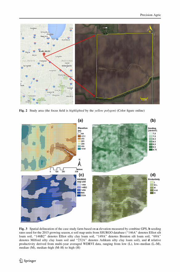
Fig. 2 Study area (the focus field is highlighted by the yellow polygon) (Color figure online)

Fig. 3 Spatial delineation of the case study farm based on a elevation measured by combine GPS, b seedingrates used for the 2015 growing season, c soil map units from SSURGO database (‘‘146A’’ denotes Elliot siltloam soil, ‘‘146B2’’ denotes Elliot silty clay loam soil, ‘‘149A’’ denotes Brenton silt loam soil, ‘‘69A’’denotes Milford silty clay loam soil and ‘‘232A’’ denotes Ashkum silty clay loam soil), and d relativeproductivity derived from multi-year averaged WDRVI data, ranging from low (L), low–median (L–M),median (M), median–high (M–H) to high (H)

Precision Agric

123

Results and discussion

Management zone delineation

The delineation of relative productivity zones derived from the 5-year averaged summer

time WDRVI is shown in Fig. 3d. High productivity zones accounted for 24.3% of the

whole field, and were found mainly in the northwest and southeast parts of the field. Low

productivity zones accounted for 9.6%, and distributed as a striped channel stretching from

the southeast to the middle of the field. Such a channel was also identified from the Google

Earth bare soil imagery (Fig. 2). High–median, median and median–low productivity

zones accounted for 26.7, 23.1 and 16.3%, respectively. Sub-field variability of produc-

tivity zones was comparable to bare soil colors, with high productivity zones generally

occurring in light colored soils and low productivity zones corresponding to dark soils

(Figs. 2, 3d). Such a spatial pattern contrasted the prevalent expectation that darker soils

with more SOM in general had higher fertility (e.g. Ladoni et al. 2010; Scharf 2015). One

possible explanation is that dark-colored soils were prone to flooding as they had on

average lower elevation than surrounding areas (Fig. 3a), thus receiving little benefit from

greater humus accumulation. It is also likely that the spectral properties of surface soils

may not reflect the fertility of deeper soils. These speculations echo Fleming et al. (2004),

who found that management zones retrieved from soil colors differed substantially from

the results derived from the soil apparent electrical conductivity (ECa), and the latter

approach was more effective in identifying the expected spatial variability in a case study.

The configuration of satellite derived productivity zones were not consistent with the

SSURGO soil map (Fig. 3c, d), suggesting more efforts are required to transfer soil survey

data into directly usable information for sub-field precision management. The final man-

agement zones generated by overlaying soil types and productivity zones are presented in

Fig. S1.

Management zone delineation was so far a critically uncertain step of this prototype. To

date, an efficient and accurate procedure for creating management zones is still lacking,

and no single method fits all situations (Derby et al. 2007). This study utilized the satellite

imagery of crop growth to delineate the management zones, mainly because of the effi-

ciency and scalability of this approach. Canopy sensor- or grid soil sampling-based

approaches for in-season N recommendation may be more reliable as they are based on

field measurements, but the considerable labor cost negates the accuracy (Scharf 2015).

Soil ECa is more cost-effective than the traditional fieldwork based approach, whereas its

interpretation often requires the use of additional georeferenced data and expert experi-

ence. In cases of low yield due to unfavorable weather conditions, the economic benefit

from ECa measurement may not outcompete the costs (Derby et al. 2007). Topography

(e.g. elevation) has long been identified as a yield-limiting factor (Kravchenko and Bullock

2000). With the advent of high-quality topographic data, soil survey databasse in con-

junction with terrain attributes such as elevation, topographic wetness index, slope per-

centage and modified catchment area can be used to generate digital maps that better

represent the soil functions (Ashtekar and Owens 2013; Chaney et al. 2016). Future

research efforts will focus on integrating the geospatial information of soil reflectance and

topography into the management zone delineation.

Precision Agric

123

Soil parameter sensitivity and LAI calibration

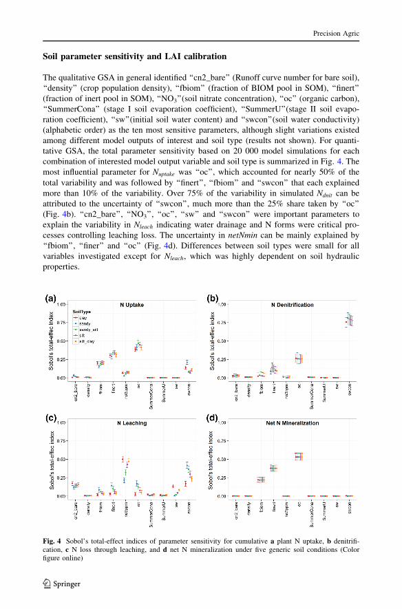
The qualitative GSA in general identified ‘‘cn2_bare’’ (Runoff curve number for bare soil),

‘‘density’’ (crop population density), ‘‘fbiom’’ (fraction of BIOM pool in SOM), ‘‘finert’’

(fraction of inert pool in SOM), ‘‘NO3’’(soil nitrate concentration), ‘‘oc’’ (organic carbon),

‘‘SummerCona’’ (stage I soil evaporation coefficient), ‘‘SummerU’’(stage II soil evapo-

ration coefficient), ‘‘sw’’(initial soil water content) and ‘‘swcon’’(soil water conductivity)

(alphabetic order) as the ten most sensitive parameters, although slight variations existed

among different model outputs of interest and soil type (results not shown). For quanti-

tative GSA, the total parameter sensitivity based on 20 000 model simulations for each

combination of interested model output variable and soil type is summarized in Fig. 4. The

most influential parameter for Nuptake was ‘‘oc’’, which accounted for nearly 50% of the

total variability and was followed by ‘‘finert’’, ‘‘fbiom’’ and ‘‘swcon’’ that each explained

more than 10% of the variability. Over 75% of the variability in simulated Ndnit can be

attributed to the uncertainty of ‘‘swcon’’, much more than the 25% share taken by ‘‘oc’’

(Fig. 4b). ‘‘cn2_bare’’, ‘‘NO3’’, ‘‘oc’’, ‘‘sw’’ and ‘‘swcon’’ were important parameters to

explain the variability in Nleach indicating water drainage and N forms were critical pro-

cesses controlling leaching loss. The uncertainty in netNmin can be mainly explained by

‘‘fbiom’’, ‘‘finer’’ and ‘‘oc’’ (Fig. 4d). Differences between soil types were small for all

variables investigated except for Nleach, which was highly dependent on soil hydraulic

properties.

Fig. 4 Sobol’s total-effect indices of parameter sensitivity for cumulative a plant N uptake, b denitrifi-cation, c N loss through leaching, and d net N mineralization under five generic soil conditions (Colorfigure online)

Precision Agric

123

Sensitivity analysis demonstrated that soil water conductivity and the amount and

composition of SOC are the most sensitive parameters to explain the variability in each of

the model outputs of interest. Apart from the soil parameters investigated in the GSA, the

importance of hydraulic parameters such as saturated water content (SAT in APSIM),

water holding capacity (DUL in APSIM) and wilting point (LL15 in APSIM) to all above-

mentioned processes are well established as well (Tremblay et al. 2012; Scharf 2015).

These hydraulic parameters, along with soil water conductivity, have a robust relationship

with soil texture (Saxton and Rawls 2006). Therefore, the uncertainty of the in-season N

recommendation can be well constrained if there is better knowledge about the within-field

heterogeneity of SOC and soil texture, both of which are more likely to be estimated in a

scalable way (Mulder et al. 2011; Castaldi et al. 2016).

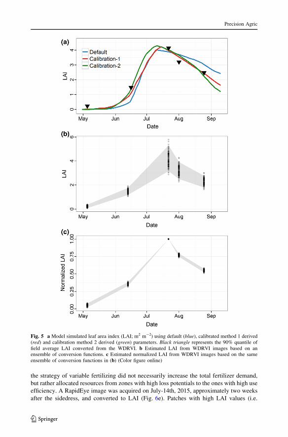
By using the SCEM-UA method, Calibration-1 improved the 2014 LAI simulation,

especially for the V5/V6 stage when rapid canopy growth starts in response to a high rate

of N uptake (Fig. 5a). The root mean square error (RMSE) decreased from 0.526 m2 m-2

for the simulations with default parameters to 0.258 m2 m-2 for the optimized set. For the

2015 growing season, using the optimized parameters increased the simulated field average

LAI on June 22nd from 0.053 to 0.269 (LAI curve not shown), and hence three times more

plant N uptake than simulations with default parameters. The normalized LAI based on the

Calibration-2 method was slightly more efficient than using the Calibration-1 method in

matching the early season LAI given the same number of SCEM-UA runs (Fig. 5a),

although they were almost equal in optimizing the RMSE of the whole season LAI

observations (0.258 for Calibration-1 vs. 0.259 for Calibration-2). The calibration method

showed that assimilating WDRVI data into the APSIM model can reduce the uncertainty in

LAI simulation, which further improves the prediction of crop growth and N uptake.

Interestingly, estimating LAI by variants of Eq. 5 generated high uncertainties, especially

around the period of peak canopy growth (Fig. 5b). Yet normalized LAI was much less

affected by the selection of a specific Eq. 5 variant (Fig. 5c). This contrast implied that

uncertainties associated with the estimation of LAI from WDRVI images can be effec-

tively reduced by using normalized LAI.

Sub-field sidedress recommendation

By the time that N sidedress was requested, Nloss via denitrification and leaching for the

farm was considerable (Fig. 6a), accounting for an average of 20% of the spring N

application. Sub-field variations were mostly delineated by soil types (Fig. 3b). However,

the highest loss mainly came from the Ashkum silty clay loam soil (map unit 232A) with

greater SOM, suggesting greater spring mineralization might have led to greater N loss

under certain conditions. The variations in Nuptake were small, with the majority grids

showing N uptake between 20 and 25 kg ha-1 N (Fig. 6b), indicating substantial N uptake

had not yet happened at this stage. The spatial patterns of Nuptake did not follow either soil

types or management zones, yet were close to the seeding rates (Fig. 3b). Grids with denser

corn population in general showed more N uptake. The sub-field variability of Nleftover was

primarily characterized by indigenous soil supply potential, while Nloss and Nuptake played

secondary roles (Fig. 6c). The recommended Nsidedress rates followed the management zone

distribution (Fig. S1), with secondary variability further identified by other factors

(Fig. 6d). Very high rates ([120 kg ha-1) accounted for 8.1% of the total field, because

these parts had high yield potential. The field average sidedress rate was 92.8 kg ha-1, and

was close to the difference between the Ntarget and flat rate of pre-plant application. Thus

Precision Agric

123

the strategy of variable fertilizing did not necessarily increase the total fertilizer demand,

but rather allocated resources from zones with high loss potentials to the ones with high use

efficiency. A RapidEye image was acquired on July-14th, 2015, approximately two weeks

after the sidedress, and converted to LAI (Fig. 6e). Patches with high LAI values (i.e.

Fig. 5 a Model simulated leaf area index (LAI; m2 m-2) using default (blue), calibrated method 1 derived(red) and calibration method 2 derived (green) parameters. Black triangle represents the 90% quantile offield average LAI converted from the WDRVI. b Estimated LAI from WDRVI images based on anensemble of conversion functions. c Estimated normalized LAI from WDRVI images based on the sameensemble of conversion functions in (b) (Color figure online)

Precision Agric

123

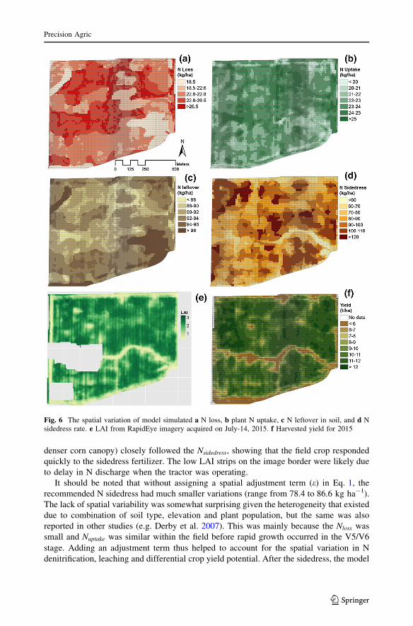
denser corn canopy) closely followed the Nsidedress, showing that the field crop responded

quickly to the sidedress fertilizer. The low LAI strips on the image border were likely due

to delay in N discharge when the tractor was operating.

It should be noted that without assigning a spatial adjustment term (e) in Eq. 1, the

recommended N sidedress had much smaller variations (range from 78.4 to 86.6 kg ha-1).

The lack of spatial variability was somewhat surprising given the heterogeneity that existed

due to combination of soil type, elevation and plant population, but the same was also

reported in other studies (e.g. Derby et al. 2007). This was mainly because the Nloss was

small and Nuptake was similar within the field before rapid growth occurred in the V5/V6

stage. Adding an adjustment term thus helped to account for the spatial variation in N

denitrification, leaching and differential crop yield potential. After the sidedress, the model

Fig. 6 The spatial variation of model simulated a N loss, b plant N uptake, c N leftover in soil, and d Nsidedress rate. e LAI from RapidEye imagery acquired on July-14, 2015. f Harvested yield for 2015

Precision Agric

123

could be run progressively by assimilating new weather data and monitoring the soil and

crop N state throughout the remaining growing season to alert N stress occurrences.

The harvested yield for 2015 differed substantially within the field, with low yield

patches amounting to less than 6 t ha-1 and highest yield up to 12.8 t ha-1 (Fig. 6f). The

spatial variability in yield was comparable with variable sidedress rates (Fig. 6d), with

greater yield occurring in places where greater sidedress N was applied. The low yield strip

stretching from southeast to west is also easily identified, matching closely to the low

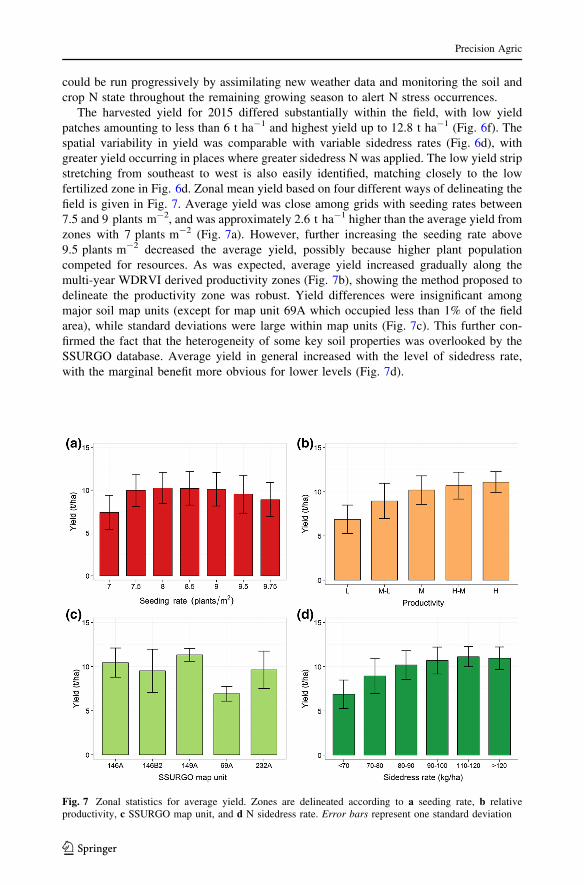
fertilized zone in Fig. 6d. Zonal mean yield based on four different ways of delineating the

field is given in Fig. 7. Average yield was close among grids with seeding rates between

7.5 and 9 plants m-2, and was approximately 2.6 t ha-1 higher than the average yield from

zones with 7 plants m-2 (Fig. 7a). However, further increasing the seeding rate above

9.5 plants m-2 decreased the average yield, possibly because higher plant population

competed for resources. As was expected, average yield increased gradually along the

multi-year WDRVI derived productivity zones (Fig. 7b), showing the method proposed to

delineate the productivity zone was robust. Yield differences were insignificant among

major soil map units (except for map unit 69A which occupied less than 1% of the field

area), while standard deviations were large within map units (Fig. 7c). This further con-

firmed the fact that the heterogeneity of some key soil properties was overlooked by the

SSURGO database. Average yield in general increased with the level of sidedress rate,

with the marginal benefit more obvious for lower levels (Fig. 7d).

Fig. 7 Zonal statistics for average yield. Zones are delineated according to a seeding rate, b relativeproductivity, c SSURGO map unit, and d N sidedress rate. Error bars represent one standard deviation

Precision Agric

123

Uncertainty and potential improvements

The estimation of e and expected yield

When estimating the target N rate using Eq. 1, user input of Y is preferred because growers

often know average yield for their field. The more challenging part was to estimate the

productivity adjustment term, e, which is one of the key drivers in creating a wide range of

N sidedress rate. In the case study, values for e were derived from multi-year yield maps,

which may not be easily available under most circumstances. The simplest one step for-

ward is to estimate the relative productivity directly based on the averaged multi-year

growing season WDRVI values for each productivity zone, since the empirical relationship

between corn yield and WDRVI information has proved robust for the US Corn-Belt (e.g.

Sakamoto et al. 2014). Moreover, a number of scalable methods that do not require field-

based measurements can be potentially implemented to estimate the within-field variation

in crop productivity and hence soil fertility. These approaches either relate yield to the

absorbed photosynthetically active radiation (APAR) (which can be estimated from

satellite data) and light use efficiency (LUE) or regression relationships between remotely

sensed vegetation indices and crop yield. A good summary is given in Sibley et al. (2014),

among which the approach (named Scalable Crop Yield Mapper, SCYM here after)

introduced by Lobell et al. (2015) is most promising since it requires the least number of

satellite images and almost no ground-based information and can provide estimates with

very high spatial resolution. The SCYM approach uses simulated ensemble of LAI and

yield by crop models as pseudo-observations to train a regression that relates final crop

yield to satellite observable vegetation indices and a few growing season key meteoro-

logical variables. When applying the regression for the field, the current version of SCYM

only requires satellite observations for two dates that are not too far away (e.g. 40 days)

from the peak growing season. Although not accurate enough for an individual year, the

estimation derived from the SCYM approach is much less uncertain for the multi-year

averaged yield. These features makes SCYM a promising fit to the current framework that

is built on the high spatial resolution RapidEye images that cover multiple years yet are

temporally sparse.

Assimilate satellite images to improve model performance

One caveat to be mentioned is that the number of WDRVI images used for LAI calibration

is only a little more than the number of parameters to be calibrated, thus lowering the

credibility and efficiency of our calibration. The limited number of image acquisitions was

mainly because of the bad weather conditions and the budget cap for developing this

prototype, but can be potentially solved by increasing the temporal frequency of image

request. In fact, the RapidEye constellation allows for daily revisit upon request through

off-nadir but low view angle (never exceed 20�) observation, although weekly collection

may be sufficient for LAI calibration. This feature is utilized by an updated version

(personal communication) of the Agriculture Information Service Platform introduced in

Honda et al. (2014). In the coming years, new commercial satellite systems will deliver

even better images that can overcome both spatial and temporal scaling challenges in the

near future (e.g. the PlanetScope Satellite Constellation). Alternatively, more detailed and

frequent canopy information can be obtained through the UAV-based multiple-spectral

imaging (Hunt et al. 2008), although it is not yet clear when a UAV system that has the

Precision Agric

123

capability to serve the demand from a large geographic span (e.g. the US Corn-Belt) will

become available. Once more spectral information is available, the proposed tool can be

easily adapted to do LAI calibration for the current growing season rather than the previous

year as presented in the case study. In addition, crop model estimations for both the above

ground (e.g. biomass, LAI and crop N uptake) and below ground variables (e.g. soil

moisture and hydraulic properties) can be improved by using the existing data assimilation

and inverse modeling techniques (Charoenhirunyingyos et al. 2011; Machwitz et al. 2014;

Hank et al. 2015).

Soil heterogeneity

As is shown in the sensitivity analysis, soil texture and SOM are vital to the uncertainty of

the in-season N recommendation. In the case study, using local soil sampling data for mode

calibration was not tested, because it is inefficient and not scalable. Abundant continuous

soil moisture observations at different soil depth are available from stations affiliated with

various networks (e.g. AmeriFlux, llinois, USA Climate Network and ISU Soil Moisture

Network). However, their limited spatial distribution, along with considerable soil

heterogeneity, make them unsuitable for directly comparing model simulated soil moisture

for a particular site to any measurements from a neighboring station (not to mention the

nearest station is usually miles away). One possible way to use these measurements is to do

calibration at individual sites and then extrapolate the optimized parameters based on their

relationships with more easily accessible information such as soil texture. However, the

numerical uncertainty introduced in the calibration procedures may jeopardize this method,

making it no better than using empirical relationships provided in the literature. For

example, Saxton et al. (1986) introduced a method (Saxton method hereafter) to estimate

generalized soil hydraulic characteristics from soil texture, and released an updated version

with additional field measurements (Saxton and Rawls 2006). When comparing soil

hydraulic parameters calculated by the Saxton method to values obtained from SSURGO,

the two sets had similar values. In addition, as is discussed in the previous section, these

parameters can be estimated based on aboveground information using inverse modeling

techniques (Charoenhirunyingyos et al. 2011). Determining SOC is even more challenging,

because the traditional soil sampling is labor and cost intensive and suffers from a high

spatial uncertainty (Scharf 2015). Simple, reliable and scalable methods to estimate the

spatial heterogeneity in SOC are still lacking. Soil reflectance (color) has the potential to

fill this gap, but results obtained using this method so far can be only treated as preliminary

(Gomez et al. 2008; Ladoni et al. 2010). In addition, some recent studies show the potential

to fine tune SSURGO data based on layers of information such as topography (Ashtekar

and Owens 2013; Chaney et al. 2016) and hyperspectral imagery.

Conclusions

This study presented a sub-field scale prescription tool for variable rate N fertilization for

the US Corn system. The proposed tool employed the crop model simulations to track a

range of soil N processes, and used satellite images to derive management zones, to train

the crop model and to assess the crop growth status. In a case study, the tool successfully

captured the sub-field variability of crop systems. The recommended sidedress N rates

enhanced zones with high yield potential, while preventing over-fertilization in zones with

Precision Agric

123

low yield potential. Marginal benefits from sidedress decreased with the increase of fer-

tilizer amount. Model sensitivity analysis indicated that soil hydraulic properties and soil

organic carbon content are critical to the reliability of this sidedress N recommendation

tool. Crop N uptake at the time of sidedress can be well constrained by calibrating the

phenology module using normalized satellite-derived LAI. Compared with other N rec-

ommendation tools, the framework presented here is efficient, accurate and scalable and

requires less upfront information from users.

Although the prototype introduced in this study can be easily adapted to other crops or

regions outside the US, two caveats should be noted. First, information on soil properties is

the major source of uncertainty. When abundant aerial images are available (either through

satellite or UAV), estimating a few soil parameters using inverse modeling approaches is

worth considering. Alternatively, it is desirable to better extrapolate or fine tune existing

soil survey data based on layers of information such as ECa, topography and aerial ima-

gery. Second, the performance of the proposed tool is highly relevant to the number of

RapidEye images that can be acquired within a growing season. Higher frequency of image

collection is highly recommended to further improve this tool. This can be achieved by

requesting smaller revisit time from the RapidEye system, by switching to other imagery

sources such as the PlanetScope Satellite Constellation, or by using the more manageable

UAV monitoring.

Acknowledgement We thank the Backend team at FarmLogs and the Information Technology at PurdueResearch Computing (RCAC) for computing support. This study is financially supported through projectsfunded to Q. Zhuang by the NASA Land Use and Land Cover Change program (NASA-NNX09AI26G), theNSF Division of Information and Intelligent Systems (NSF-1028291).

References

Abendroth, L. J. (2011). Corn growth and development. Ames, IA: Iowa State University Extension.Archontoulis, S. V., Miguez, F. E., & Moore, K. J. (2014). Evaluating APSIM maize, soil water, soil

nitrogen, manure, and soil temperature modules in the Midwestern United States. Agronomy Journal,106, 1025–1040.

Arthur, D., & Vassilvitskii, S. (2007). k-means??: The advantages of careful seeding. In Proceedings of theeighteenth annual ACM-SIAM symposium on Discrete algorithms (pp. 1027–1035). New Orleans, LS,USA: Society for Industrial and Applied Mathematics.

Ashtekar, J. M., & Owens, P. R. (2013). Remembering knowledge: An expert knowledge based approach todigital soil mapping. Soil Horizons, 54, 1–6.

Cassman, K. G., Dobermann, A., & Walters, D. T. (2002). Agroecosystems, nitrogen-use efficiency, andnitrogen management. AMBIO: A Journal of the Human Environment, 31, 132–140.

Castaldi, F., Palombo, A., Santini, F., Pascucci, S., Pignatti, S., & Casa, R. (2016). Evaluation of thepotential of the current and forthcoming multispectral and hyperspectral imagers to estimate soiltexture and organic carbon. Remote Sensing of Environment, 179, 54–65.

Chander, G., Haque, M. O., Sampath, A., Brunn, A., Trosset, G., Hoffmann, D., et al. (2013). Radiometricand geometric assessment of data from the RapidEye constellation of satellites. International Journalof Remote Sensing, 34, 5905–5925.

Chaney, N. W., Wood, E. F., McBratney, A. B., Hempel, J. W., Nauman, T. W., Brungard, C. W., et al.(2016). POLARIS: A 30-meter probabilistic soil series map of the contiguous United States. Geo-derma, 274, 54–67.

Charoenhirunyingyos, S., Honda, K., Kamthonkiat, D., & Ines, A. V. (2011). Soil moisture estimation frominverse modeling using multiple criteria functions. Computers and Electronics in Agriculture, 75,278–287.

Cicore, P., Serrano, J., Shahidian, S., Sousa, A., Costa, J. L., & da Silva, J. R. M. (2016). Assessment of thespatial variability in tall wheatgrass forage using LANDSAT 8 satellite imagery to delineate potentialmanagement zones. Environmental Monitoring and Assessment, 188, 513.

Precision Agric

123

Derby, N. E., Casey, F. X. M., & Franzen, D. W. (2007). Comparison of nitrogen management zonedelineation methods for corn grain yield. Agronomy Journal, 99, 405–414.

Diker, K., Heermann, D. F., & Brodahl, M. K. (2004). Frequency analysis of yield for delineating yieldresponse zones. Precision Agriculture, 5, 435–444.

Fleming, K. L., Heermann, D. F., & Westfall, D. G. (2004). Evaluating soil color with farmer input andapparent soil electrical conductivity for management zone delineation. Agronomy Journal, 96,1581–1587.

Gitelson, A. A. (2004). Wide dynamic range vegetation index for remote quantification of biophysicalcharacteristics of vegetation. Journal of Plant Physiology, 161, 165–173.

Gomez, C., Viscarra Rossel, R. A., & McBratney, A. B. (2008). Soil organic carbon prediction by hyper-spectral remote sensing and field vis-NIR spectroscopy: An Australian case study. Geoderma, 146,403–411.

Guastaferro, F., Castrignano, A., De Benedetto, D., Sollitto, D., Troccoli, A., & Cafarelli, B. (2010). Acomparison of different algorithms for the delineation of management zones. Precision Agriculture,11, 600–620.

Hammer, G. L., Dong, Z., McLean, G., Doherty, A., Messina, C., Schussler, J., et al. (2009). Can Changes incanopy and/or root system architecture explain historical maize yield trends in the U.S. Corn Belt?Crop Science, 49, 299–312.

Hank, T. B., Bach, H., & Mauser, W. (2015). Using a remote sensing-supported hydro-agroecological modelfor field-scale simulation of heterogeneous crop growth and yield: Application for wheat in centralEurope. Remote Sensing, 7, 3934–3965.

Holzworth, D. P., Huth, N. I., deVoil, P. G., et al. (2014). APSIM—evolution towards a new generation ofagricultural systems simulation. Environmental Modelling and Software, 62, 327–350.

Honda, K., Ines, A. V., Yui, A., Witayangkurn, A., Chinnachodteeranun, R., & Teeravech, K. (2014).Agriculture information service built on geospatial data infrastructure and crop modeling. In Pro-ceedings of the 2014 international workshop on web intelligence and smart sensing (pp. 1–9). NewYork, USA: Association for Computing Machinery.

Hunt, E. R., Hively, W. D., Daughtry, C. S., McCarty, G. W., Fujikawa, S. J., Ng, T. L., et al. (2008).Remote sensing of crop leaf area index using unmanned airborne vehicles. In Proceedings of thePecora 17 symposium. Bethesda, MD: American Society for Photogrammetry and Remote Sensing.CDROM. http://www.asprs.org/a/publications/proceedings/pecora17/0018.pdf. Accessed 31 Oct 2016.

Irish, R. R. (2000). Landsat 7 automatic cloud cover assessment. In AeroSense 2000 (pp. 348–355).Bellingham, WA, USA: International Society for Optics and Photonics.

Jin, Z., Zhuang, Q., He, J.-S., Zhu, X., & Song, W. (2015). Net exchanges of methane and carbon dioxide onthe Qinghai-Tibetan Plateau from 1979 to 2100. Environmental Research Letters, 10, 085007.

Jin, Z., Zhuang, Q., Tan, Z., Dukes, J. S., Zheng, B., & Melillo, J. M. (2016). Do maize models capture theimpacts of heat and drought stresses on yield? Using algorithm ensembles to identify successfulapproaches. Global Change Biology, 22, 3112–3126.

Keeney, D., & Olson, R. A. (1986). Sources of nitrate to ground water. Critical Reviews in EnvironmentalControl, 16, 257–304.

Kravchenko, A. N., & Bullock, D. G. (2000). Correlation of corn and soybean grain yield with topographyand soil properties. Agronomy Journal, 92, 75–83.

Ladoni, M., Bahrami, H., Alavipanah, S., & Norouzi, A. (2010). Estimating soil organic carbon from soilreflectance: A review. Precision Agriculture, 11, 82–99.

Littleboy, M., Silburn, D. M., Freebairn, D. M., Woodruff, D. R., Hammer, G. L., & Leslie, J. K. (1992).Impact of soil erosion on production in cropping systems. I. Development and validation of a simu-lation model. Soil Research, 30, 757–774.

Lobell, D. B., Hammer, G. L., McLean, G., Messina, C., Roberts, M. J., & Schlenker, W. (2013). Thecritical role of extreme heat for maize production in the United States. Nature Climate Change, 3,497–501.

Lobell, D. B., Thau, D., Seifert, C., Engle, E., & Little, B. (2015). A scalable satellite-based crop yieldmapper. Remote Sensing of Environment, 164, 324–333.

Ma, B. L., & Biswas, D. K. (2015). Precision nitrogen management for sustainable corn production. InSustainable agriculture reviews (pp. 33–62). Cham, Switzerland: Springer International Publishing.

Machwitz, M., Giustarini, L., Bossung, C., Frantz, D., Schlerf, M., Lilienthal, H., et al. (2014). Enhancedbiomass prediction by assimilating satellite data into a crop growth model. Environmental Modellingand Software, 62, 437–453.

Mamo, M., Malzer, G. L., Mulla, D. J., Huggins, D. R., & Strock, J. (2003). Spatial and temporal variation ineconomically optimum nitrogen rate for corn. Agronomy Journal, 95, 958–964.

Precision Agric

123

McIsaac, G. F., David, M. B., Gertner, G. Z., & Goolsby, D. A. (2002). Relating net nitrogen input in theMississippi River Basin to nitrate flux in the lower Mississippi River. Journal of EnvironmentalQuality, 31, 1610–1622.

Melkonian, J. J., van Es, H. M., DeGaetano, A. T., & Joseph, T. (2008) ADAPT-N: Adaptive nitrogenmanagement for maize using high resolution climate data and model simulations. In: R. Khosla (Ed.),Proceedings of the 9th international conference on precision agriculture. Denver, CO. 18–21 July2010. Monticello, IL, USA: International Society of Precision Agriculture. CDROM.

Moebius-Clune, B., Van Es, H., & Melkonian, J. (2013). Adapt-N uses models and weather data to improvenitrogen management for corn. Better Crops, 97, 7–9.

Mulder, V. L., De Bruin, S., Schaepman, M. E., & Mayr, T. R. (2011). The use of remote sensing in soil andterrain mapping—a review. Geoderma, 162, 1–19.

Mulla, D. J. (2013). Twenty five years of remote sensing in precision agriculture: Key advances andremaining knowledge gaps. Biosystems Engineering, 114, 358–371.

Pappas, C., Fatichi, S., Leuzinger, S., Wolf, A., & Burlando, P. (2013). Sensitivity analysis of a process-based ecosystem model: Pinpointing parameterization and structural issues. Journal of GeophysicalResearch: Biogeosciences, 118, 505–528.

Park, S., Croteau, P., Boering, K. A., Etheridge, D. M., Ferretti, D., Fraser, P. J., et al. (2012). Trends andseasonal cycles in the isotopic composition of nitrous oxide since 1940. Nature Geoscience, 5,261–265.

Prasad, R., Hochmuth, G. J., & Boote, K. J. (2015). Estimation of nitrogen pools in irrigated potatoproduction on sandy soil using the model SUBSTOR. PLoS ONE, 10, e0117891.

Randall, G. W., Vetsch, J. A., & Huffman, J. R. (2003). Nitrate losses in subsurface drainage from a corn-soybean rotation as affected by time of nitrogen application and use of nitrapyrin. Journal of Envi-ronmental Quality, 32, 1764–1772.

Sakamoto, T., Gitelson, A. A., & Arkebauer, T. J. (2014). Near real-time prediction of US corn yields basedon time-series MODIS data. Remote Sensing of Environment, 147, 219–231.

Saxton, K. E., & Rawls, W. J. (2006). Soil water characteristic estimates by texture and organic matter forhydrologic solutions. Soil Science Society of America Journal, 70, 1569–1578.

Saxton, K. E., Rawls, W. J., Romberger, J. S., & Papendick, R. I. (1986). Estimating generalized soil-watercharacteristics from texture. Soil Science Society of America Journal, 50, 1031–1036.

Scharf, P. C. (2015) Managing nitrogen. In: Managing nitrogen in crop production (pp. 25–76). Madison,WI, USA: American Society of Agronomy, Inc., Crop Science Society of America, Inc., and SoilScience Society of America, Inc.

Sela, S., van Es, H. M., Moebius-Clune, B. N., Marjerison, R., Melkonian, J., Moebius-Clune, D., et al.(2016). Adapt-N outperforms grower-selected nitrogen rates in Northeast and Midwestern UnitedStates strip trials. Agronomy Journal, 103(108), 1726–1734.

Setiyono, T. D., Yang, H., Walters, D. T., Dobermann, A., Ferguson, R. B., Roberts, D. F., et al. (2011).Maize-N: A Decision tool for nitrogen management in maize. Agronomy Journal, 103, 1276–1283.

Shaddad, S. M., Madrau, S., Castrignano, A., & Mouazen, A. M. (2016). Data fusion techniques fordelineation of site-specific management zones in a field in UK. Precision Agriculture, 17, 200–217.

Shahandeh, H., Wright, A. L., & Hons, F. M. (2011). Use of soil nitrogen parameters and texture forspatially-variable nitrogen fertilization. Precision Agriculture, 12, 146–163.

Sibley, A. M., Grassini, P., Thomas, N. E., Cassman, K. G., & Lobell, D. B. (2014). Testing remote sensingapproaches for assessing yield variability among maize fields. Agronomy Journal, 106, 24–32.

Sinclair, T. R., & Muchow, R. C. (1995). Effect of nitrogen supply on maize yield: I. Modeling physio-logical responses. Agronomy Journal, 87, 632–641.

Soil Survey Staff, Natural Resources Conservation Service, United States Department of Agriculture. WebSoil Survey. Retrieved Octobor 31, 2016 from http://websoilsurvey.nrcs.usda.gov/.

Solie, J. B., Monroe, A. D., Raun, W. R., & Stone, M. L. (2012). Generalized algorithm for variable-ratenitrogen application in cereal grains. Agronomy Journal, 104, 378–387.

Song, X., Wang, J., Huang, W., Liu, L., Yan, G., & Pu, R. (2009). The delineation of agricultural man-agement zones with high resolution remotely sensed data. Precision Agriculture, 10, 471–487.

Thompson, L. J., Ferguson, R. B., Kitchen, N., Frazen, D. W., Mamo, M., Yang, H., et al. (2015). Model andsensor-based recommendation approaches for in-season nitrogen management in corn. AgronomyJournal, 107, 2020–2030.

Tibshirani, R., Walther, G., & Hastie, T. (2001). Estimating the number of clusters in a data set via the gapstatistic. Journal of the Royal Statistical Society: Series B (Statistical Methodology), 63, 411–423.

Tremblay, N., Bouroubi, Y. M., Belec, C., Mullen, R. W., Kitchen, N. R., Thomason, W. E., et al. (2012).Corn response to nitrogen is influenced by soil texture and weather. Agronomy Journal, 104,1658–1671.

Precision Agric

123

Vina, A., Gitelson, A. A., Nguy-Robertson, A. L., & Peng, Y. (2011). Comparison of different vegetationindices for the remote assessment of green leaf area index of crops. Remote Sensing of Environment,115, 3468–3478.

Wilson, D. R., Muchow, R. C., & Murgatroyd, C. J. (1995). Model analysis of temperature and solarradiation limitations to maize potential productivity in a cool climate. Field crops research, 43, 1–18.

Yang, H., Dobermann, A., Cassman, K. G., & Walters, D. T. (2006). Features, applications, and limitationsof the Hybrid-Maize simulation model. Agronomy Journal, 98, 737–748.

Zhang, X., Shi, L., Jia, X., Seielstad, G., & Helgason, C. (2010). Zone mapping application for precision-farming: A decision support tool for variable rate application. Precision Agriculture, 11, 103–114.

Precision Agric

123