critical values for the two independent samples piper …
TRANSCRIPT

CRITICAL VALUES FOR THE TWO INDEPENDENT SAMPLES WINSORIZED T TEST
by
PIPER A. FARRELL-SINGLETON
DISSERTATION
Submitted to the Graduate School
of Wayne State University,
Detroit, Michigan
in partial fulfillment of the requirements
for the degree of
DOCTOR OF PHILOSOPHY
2010
MAJOR: EDUCATION, EVALUATION
AND RESEARCH
Approved by:
___________________________________
Advisor Date
___________________________________
___________________________________
___________________________________

UMI Number: 3412108
All rights reserved
INFORMATION TO ALL USERS The quality of this reproduction is dependent upon the quality of the copy submitted.
In the unlikely event that the author did not send a complete manuscript
and there are missing pages, these will be noted. Also, if material had to be removed, a note will indicate the deletion.
UMI 3412108
Copyright 2010 by ProQuest LLC. All rights reserved. This edition of the work is protected against
unauthorized copying under Title 17, United States Code.
ProQuest LLC 789 East Eisenhower Parkway
P.O. Box 1346 Ann Arbor, MI 48106-1346

©COPYRIGHT BY
PIPER FARRELL-SINGLETON
2010
All Rights Reserved

ii
DEDICATION
To my family, my friends and The Most High God.

iii
ACKNOWLEDGEMENTS
I would like to first give honor to God, for without Him, this work would not have been
possible. Second, I would like to thank my mother, the late Marie Farrell-Donaldson, whose
courage and ability to face the unknown inspired me to pursue this work. To my grandmother,
Lorine “Mother Love” Morgan, your love and encouragement are invaluable. To my precious
daughter, Aris Singleton, who helped keep me focused; To my stepfather, Dr. Clinton L.
Donaldson, thank you for inspiring me to use education as a key to unlock the door to my
dreams; My father, Joseph Farrell, your wisdom, love and life lessons helped me to see this
project through to the end. To my mentor, Apostle Briggie Stansberry, your unfailing love,
prayers and support helped me to realize the destiny within me. A special thanks to Howard
Booker for his much appreciated guidance, support and dedication to keeping me focused; my
advisor, Dr. Shlomo Sawilowsky, for your patience, understanding and humor; My dissertation
committee members, Dr. Gail Fahoome, Dr. Michael Addonizio and Dr. Monte Piliawsky for
your support and dedication to this project; and to the countless other friends and family
members who have waited patiently at the finish line for me- Ready or not, here I come!

iv
TABLE OF CONTENTS
Dedication ...................................................................................................................... ii
Acknowledgments......................................................................................................... iii
List of Tables .................................................................................................................. v
List of Figures ................................................................................................................ vi
CHAPTER 1 – Introduction............................................................................................ 1
CHAPTER 2 – Review of Literature .............................................................................. 9
CHAPTER 3 – Methodology ........................................................................................ 35
CHAPTER 4 – Results.................................................................................................. 40
CHAPTER 5 – Discussion ............................................................................................ 48
References ..................................................................................................................... 53
Abstract ......................................................................................................................... 61
Autobiographical Statement.......................................................................................... 62

v
LIST OF TABLES
Table 1: Efficiencies for trimmed and winsorized samples .......................................... 32
Table 2: Sample data used to verify algorithm…… ..................................................... 36
Table 3: Monte Carlo summary results for sample size n1=n2=2 ................................ 37
Table 4: Maximum winsorized values per side for the two sample winsorized t......... 38
Table 5: Critical values for the two sample winsorized t test ....................................... 43
Table 6: Random data used for comparison ................................................................. 49
Table 7: Summary of sample A and B data for n = 25 ................................................. 50

vi
LIST OF FIGURES
Figure 1: Effects of variations in the probability of occurrence of an outlier on
power functions of the Student’s t test,Zimmerman (1994) ......................... 14
Figure 2: Effects of variations in the probability of occurrence of an outlier on
power functions of the Mann-Whitney-Wilcoxon test,
Zimmerman (1994) ........................................................................................ 14
Figure 3: Probability of Type I errors of the Student t test when the null hypothesis
is true, Zimmerman (1994) ............................................................................ 16
Figure 4: Probability of Type I errors of the Mann-Whitney-Wilcoxon test
when the null hypothesis is true, Zimmerman (1994) ................................... 16
Figure 5: Weibull Distribution characteristics .............................................................. 30

1
CHAPTER 1
CRITICAL VALUES FOR THE TWO INDEPENDENT SAMPLES WINSORIZED T TEST
Introduction
According to Barnett and Lewis (1984, p. 4), an outlier is an observation (or
subset of observations), in a set of data which appears to be inconsistent with the
remainder of that set of data. One of the earliest references to outliers was suggested by
Boscovich (1755) in an attempt to determine the ellipticity of the earth by averaging
measures of excess of the polar degree over the equatorial. In his study, Boscovich
determined that two of the ten measured values exceeded the normal range. In an attempt
to obtain the best estimate of the mean, Boscovich proceeded to compute the mean minus
the two extreme scores in an effort to adjust for the effects of the outlying scores. It was
later proposed by Bernoulli (1755) that the practice of removing outliers should not be
condemned but that the determination should be left to the satisfaction of the observer
and that extreme observations should not be removed or rejected simply because they
appear inconsistent with remaining data values.
In 1838, subsequent attempts to address the presence and effects of outliers were
made by a German mathematician and astrologer named W. F. Bessel. In his work with
outliers, Bessel (1838) acknowledged that “he had never rejected an observation simply
because of its large residual, and that all completed observations should be given equal
weight and consideration and allowed to contribute to the results” (Ascombe, 1960, p.
125). Peirce (1852) later published the first objective test for anomalous observations,
which was later followed by the publication of a test for a single doubtful observation by
Chauvenet (1863). Their methodology, however, sparked much controversy until 1884

2
when Wright (1884) proposed that the best method for dealing with outliers in
astronomical readings was for the non observer to reject any observation whose residual
exceeded in magnitude five times the probable error, or 3.37 times the standard deviation
(Ascombe, 1960, p.125). Basing his reasoning on the Gaussian law of error being
satisfied, Wright (1884) succumbed that “minimal damage would be incurred due to the
fact that only about one observation in a thousand would be rejected” (Ascombe, 1960,
p.125).
Since then, identifying and treating outliers has become so critical to the study of
statistics that many suggestions have been made as to what criteria should be used to
identify outliers, as well as how they should be treated for purposes of statistical analyses.
Identification and treatment of outliers is crucial to statistical research because if left
unchecked, outliers can increase error variance, reduce the power of statistical tests,
decrease normality (if non-randomly distributed), violate assumptions of sphericity and
multivariate normality (in multivariate analyses), as well as significantly bias or influence
estimates that may be of considerable interest (Osborne & Overbay, 2004 ). With recent
advancements in modern statistical methods, however, the process of identifying and
treating outliers has become increasingly simplified.
Problem
The two sample t test is the best-known and most popular method for comparing
two groups according to Wilcox (1996). In the presence of outliers, however, the test
becomes inexact and the likelihood of Type I error inflations (or deflations) is
significantly increased. Over the years, numerous recommendations have been made as to
how to implement the two sample t test in the presence of outliers in an effort to obtain

3
the most valid and reliable statistical estimates. This decision is of particular importance
because removal of outliers has been linked to problems such as increased sampling
error, particularly when the underlying distribution is unknown or contaminated, as well
as the increased likelihood of violating underlying assumptions. These concerns can
have serious effects on the validity of statistical studies and can negatively impact
statistical results when making inferences about data. Tukey and McLaughlin (1963)
noted that procedures which fare well under normality behaved relatively poorly when
applied to longer tailed distributions. With the recent developments in statistical science,
such as computer simulations with real-world data, and a wider variation of statistical
procedures, such as nonparametric procedures, to test hypotheses, it has also become
more evident that the basic assumptions of the normality approach do not hold true in a
vast majority of situations. As a result, several attempts have been made to properly
address the effects of outliers in instances where the two sample t test is employed, while
preserving the integrity of the data and statistical analyses.
Ascombe (1960), for example, recommended that outliers be discarded when they
occur as a result of large measurement or execution errors which cannot be rectified, and
if there is no further interest in studying such errors. Osborne and Overbay (2004) on the
other hand, argued that steps taken to remedy outliers depend greatly on why they
initially exist. Judd and McClelland (1989) contended that outliers, whether legitimate or
questionable, should be removed to provide the most honest estimate of population
parameters, while others (Orr, Sackett, & DuBois, 1991) maintained that removal of
outliers should be contingent upon the training, intuition, reasoned argument, and
thoughtful consideration of the researcher before a decision is made. In recent years,

4
however, a more modern and robust statistical method called winsorization has been
proposed as a solution for the treatment of outliers, as well as preservation of the integrity
of the data.
Moir (1998) noted that early parametric procedures were often used to conduct
hypothesis tests when analyzing data. One of the most notable parametric tests for
analyzing differences between independent groups is the two sample t test. It is a well-
known fact that the presence of outliers in data sets can cause severe inflations about the
mean, which can have deleterious effects on estimators which rely on the mean such as
the variance, standard deviation, and mean squared deviations. As technology allowed
for more sophisticated means of data analysis under various treatment conditions, the
robustness of parametric procedures has become more debatable. This is particularly true
in the areas of education and psychology, where variables were once thought to
approximate the normal distribution, however recent analysis has determined this to be a
misconception. Techniques such as trimming and winsorization have often been
suggested as robust alternatives that were more effective in controlling Type I error
probabilities associated with data abnormalities, particularly when the distribution of
errors was nonnormal or unknown or when sample sizes were unusually small (Moir,
1998).
Purpose of the Study
The purpose of this study will be to implement Monte Carlo techniques in
conjunction with the two sample winsorized t test to approximate critical values for the
distribution of the winsorized t. Critical values will be generated at the 0.01 and 0.05
alpha levels for both one and two tailed tests. Prior to this study, the distribution of the

5
two sample symmetrically winsorized t was unknown and had to be approximated using
Student’s t distribution, with h1+h2-2 df, (Dixon & Tukey, 1968) where h represented the
number of unwinsorized observations. The findings of this study will offer table of
approximate critical values for the two sample independent winsorized t test.
Assumptions and Limitations
To generate the table of critical values for the winsorized t test, 1,000,000
iterations were performed for each sample size and winsorization level. The accuracy of
the critcal values generated are solely based on the number of iterations. To increase the
precision of the tabled values, the number of iterations should be incremented beyond
1,000,000.
Definition of Terms
Critical Value: The critical value(s) for a hypothesis test is a threshold to which the value
of the test statistic in a sample is compared to determine whether or not the null
hypothesis is rejected. The critical value for any hypothesis test depends on the
significance level at which the test is carried out, and whether the test is one-sided or
two-sided. (http://www.stats.gla.ac.uk/steps/glossary/hypothesis_testing.html#critval).
Degrees of Freedom (df): The degrees of freedom of an estimate, denoted by the Greek
letter nu, ν, is equal to the number of independent scores that go into the estimate minus
the number of parameters estimated as intermediate steps in the estimation of the
parameter itself.
Monte Carlo Estimation: Computer intensive method used to test the hypothesis that the
data are a random sample from a specified population (Noreen, 1989).

6
Non-normality: Used to describe values of which the frequency distribution is markedly
different from that of the normal probability distribution.
Nonparametric Statistics: Statistical techniques designed to be used when the data being
analyzed depart from the distributions that can be analyzed with parametric statistics. In
practice, this most often means data measured on a nominal or an ordinal scale. Also
called distribution-free statistics (Vogt, p.192). Statistical procedures that do not require
that samples come from populations with normal distributions or any other particular
distributions. (Triola, 2006, p. 676).
Outlier: An observation (or subset of observations), in a set of data which appears to be
inconsistent with the remainder of that set of data (Barnett & Lewis, 1984, p. 4).
Parametric Tests: Statistical procedures, based on population parameters, for testing
hypotheses or estimating parameters (Triola, 2006, p. 676). A parametric statistical test
depends on a number of assumptions about the population from which the samples used
in the test are drawn (Kerlinger & Lee, 2000, p. 414).
Robustness: Insensitivity to departures from assumptions surrounding an underlying
probabilistic model (Hoaglin, Mosteller & Tukey, 1983, p. 2).
Sample Mean: The sum of the measurements divided by the number of measurements
contained in the batch of numbers (Wilcox, 1996, p. 13).
Skewed Distribution: A distribution of scores or measures that, when plotted on a graph,
produces a nonsymmetrical curve. In a unimodal skewed frequency distribution, the
mode, mean, and median are different. When the skewness of a group of values is zero,
their distribution is symmetrical (Vogt, 1993, p. 266).

7
Significance Level: A fixed probability of wrongly rejecting the null hypothesis H0, if it
is in fact true. It is the probability of a Type I error and is set by the investigator in
relation to the consequences of such an error. The significance level should be made as
small as possible in order to protect the null hypothesis and to prevent, as far as possible,
the investigator from inadvertently making false claims. The significance level is usually
denoted by where:
Significance Level = P(Type I error) =
(Http://www.stats.gla.ac.uk/steps/glossary/hypothesis_testing.html#sl).
Trimmed mean: A measure of central tendency that allows the researcher to deal
separately with a distribution’s outlier. It is a mean computed without the extreme
observations (Vogt, 1993, p. 295).
Type I Error: Rejecting the null hypothesis (Ho) when in fact it is true. In a given
statistical test, the probability of a Type I error is equal to the alpha level (α).
Type II Error: Failing to reject the null hypothesis (Ho) when in fact it is false. In a given
statistical test, the probability of a Type II error is also known as power or beta (β).
Violation of Assumptions: Statistical hypothesis tests generally make assumptions about
the population(s) from which the data were sampled. For example, many normal-theory-
based tests such as the t test and ANOVA assume that the data are sampled from one or
more normal distributions, as well as that the variances of the different populations are
the same (homoscedasticity:). If test assumptions are violated, the test results may not be
valid.

8
(ProphetSTATGuide,http://www.basic.northwestern.edu/statguidefiles/sg_glos.html#ske
wness)
Winsorized Sample Mean: The mean which replaces the largest r observations with the
(r + 1) st largest observation and replaces the s smallest observations by the (s + 1) st
smallest.
Winsorized Sample Variance: The variance of the winsorized set of values, W,
22)(
1
1wiw
XWn
s , where n is the sample size.

9
CHAPTER 2
LITERATURE REVIEW
Overview
Outliers have been a problematic concern since the inception of statistics. One of
the first known efforts to address issues concerning outliers was made by Boscovich in
1755. In an attempt to determine the average ellipticity of the earth using polar degrees
over the equatorial, Boscovich collected ten measures. When he determined that two of
the ten measures exceeded the normal range, Boscovich removed the two extraneous
values and calculated the mean of the eight remaining values. As one of the earliest
attempts to address the presence of outliers, Boscovich set an early precedent for their
removal. As attempts to analyze data sets grew popular in several fields such as science,
psychology and education, the question of what to do with outliers began to pervade
many statistical studies.
Many researchers like Bernoulli (1775) and Bessell (1838) condemned the
practice of removing outliers simply because the scores seemed to be extreme in
comparison to the bulk of the data. Bessel (1838) argued that every data value, no matter
how extreme should be allowed to contribute to the results. Others (Bernoulli,1838; Orr,
Sackett & Dubois, 1991) also agreed that no value should be removed simply because its
magnitude was extreme in comparison to the other data values, however, they added that
any determination to remove an observation should be left to the satisfaction of the
observer. Ascombe (1960), on the other hand, suggested that outliers be removed if they
occur as a result of irreparable measurement error, and if there was no future interest in
studying the extreme value. Judd and McClelland (1989) argued to the contrary that

10
outliers should be removed to provide the most reasonable estimate of population
parameters, whether they are legitimate values or not.
With the heavy reliance on the Gaussian Theorem, distributional assumptions
were often ignored based on the assumption that all data somehow approximated the
normal distribution. Practitioners then proceeded to conduct statistical tests, ignoring the
underlying distributional assumptions, and formulating erroneous conjectures about their
findings. The failure to address the underlying distribution, as well as to adopt statistical
procedures that were impervious to outliers, led to increased sampling error, particularly
when the underlying distribution was unknown or contaminated. Tukey and McLaughlin
(1963) noted that the typical distribution of errors and fluctuations has a shape whose
tails are longer than that of a Gaussian distribution (p. 332)
Outliers also occur as a result of inherent variability (Barnett & Lewis, 1984).
Inherent variability represents occurrences that are uncontrollable and reflect the natural
distributional properties of a correct basic model which describes the generation of the
data (Barnett & Lewis, 1984, p. 26). For example, a researcher who is studying average
daily high temperatures in January in Michigan may encounter an abnormally high
reading (e.g., 63 °). Although some may be quick to dismiss this score as an illegitimate
outlier, if it is truly representative of the average high temperature readings, then it should
be included as a valid score for the sake of true statistical analysis. Barnett and Lewis
(1984) caution practitioners in labeling and dismissing all spurious scores as outliers,
noting that not all outliers are illegitimate contaminants and not all illegitimate
contaminants are outliers. With all of the aforementioned suggestions on how to address
the presence of outliers, there was no general consensus among theorists as to which

11
procedure provided the most efficient method for treatment of outliers. This made it
extremely difficult to replicate previous studies, as well as make conclusive
determinations about the validity of studies where outliers were known to exist.
Chauvenet (1863) and Peirce (1852) were the first to suggest procedures to aid in
the detection of outliers prior to analysis. Their work was proceeded by Stone (1868)
who followed with a test designed to reject outliers based on a concept of a modulus of
carelessness, m (Barnett and Lewis, 1984, p.22) and Glaisher (1873), who suggested a
procedure based on weighting. Glaisher’s method, however, was highly criticized by
Stone who later suggested another alternative method of weighting. Wright (1884)
finally suggested a more practical and still widely used method of outlier identification
which involves rejecting any observation that lies more than three standard deviations
from the mean. As more advanced methods of analysis developed, such as Monte Carlo
studies and nonparametric and robust methods, it became evident that removal of outliers
was not always a feasible approach.
Nonparametric Procedures and Robustness
Nonparametric or distribution-free procedures have often been suggested for
treatment of data where outliers are present. A nonparametric test, as defined by Bradley
(1968), is “a test which makes no hypothesis about the value of a parameter in a
statistical density function” (p.15), whereas distribution free tests “make no assumptions
about the precise form of the distribution of a population from which a sample is drawn”
(Bradley, 1968, p.15). Bradley (1968) noted that “the two definitions are not mutually
exclusive and that a test can be both nonparametric and distribution-free” (p.15). The
advantage of implementing nonparametric or distribution-free tests is the presumption

12
that the tests are robust against the effects of outliers (Andrews et al., 1972; Bradley,
1977; Stigler, 1977; Tan, 1982). Robustness against these outliers is crucial to the field
of statistics because violation of the normality assumption renders a test inexact. Bradley
(1968, 1980) was determined to discredit the use of parametric procedures as a panacea,
despite the studies of parametricians, such as Boneau (1960, 1962), Lindquist (1953) and
others who claimed that the tests such as the one-sample Z and t tests, as well as other
parametric estimators, were robust against assumption violations. Despite the arguments
posed by advocates of nonparametric procedures and the realization that outliers could
significantly affect the results of statistical tests, disagreement still continued about which
procedure was most effective in addressing outliers.
In an attempt to adequately qualify robustness, Bradley (1968) investigated the
influence of α (0.05, 0.01, or 0.001), location of rejection region (left-, right- or two-
tailed), absolute sample size (2, 4, 8, 16, 32, 64, 128, 256, 512, or 1024), relative sample
size (ratios of 1, 2, or 3), absolute population shape (L-shape or bell shape), relative
population shape (i.e. same shapes or mixed shapes), and relative population standard
deviations (ratios of 1 or 2) (p. 146). Tests were conducted on Z1, t1, Z2, t2, and Fk with K
= 3 or 4. Based on final observations from this study, Bradley (1978) surmised the
following:
For every test except t1 there was some combination of conditions for which the
liberal criterion of robustness ( │ρ - α│≤ α / 2 ) was met at N = 2 (for t1 it was not
met until N = 128), but there were also some combination for which it was not
met before N = 1024…The complexity of the combinations required for
robustness is suggested by the fact that with one unimpressive exception, there

13
was no single condition, (i.e. no α value, no rejection region, no absolute or
relative sample size, no absolute or relative shape and no relative variance) for
which the liberal criterion was always met by any of the five tests investigated,
not even if we consider only those cases in which the size of the smallest sample
was ≥ 8. The exception was that the Z2 test met the criterion under all
combinations when absolute sample size was 1024. (p. 147).
Bradley’s conclusions illuminated the behavior of some commonly employed statistical
tests under various, real conditions.
Parametric Versus Nonparametric Designs
In an attempt to boast on the effectiveness of nonparametric procedures over
parametric procedures, Zimmerman (1994) explored the effect of outliers on modified
power functions of a test and its nonparametric counterpart. Using the t test and its
nonparametric counterpart, the Mann-Whitney-Wilcoxon rank-sum test, simulations were
conducted to determine the Type I and Type II error probabilities of samples from the
mixed normal population. Each test was performed using directional significance at the
.05 significance level with 5,000 iterations for each combination of conditions. The
Student’s t test was performed first on the initial scores and the scores were then
transformed into ranks. The ranked scores were then tested based on the normal
approximation form of the Mann-Whitney-Wilcoxon rank-sum test.
14
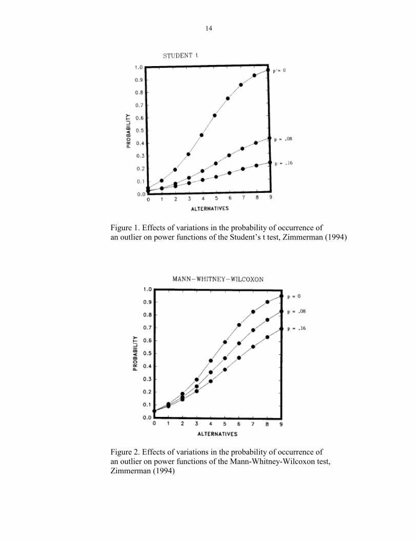
Figure 1. Effects of variations in the probability of occurrence of
an outlier on power functions of the Student’s t test, Zimmerman (1994)
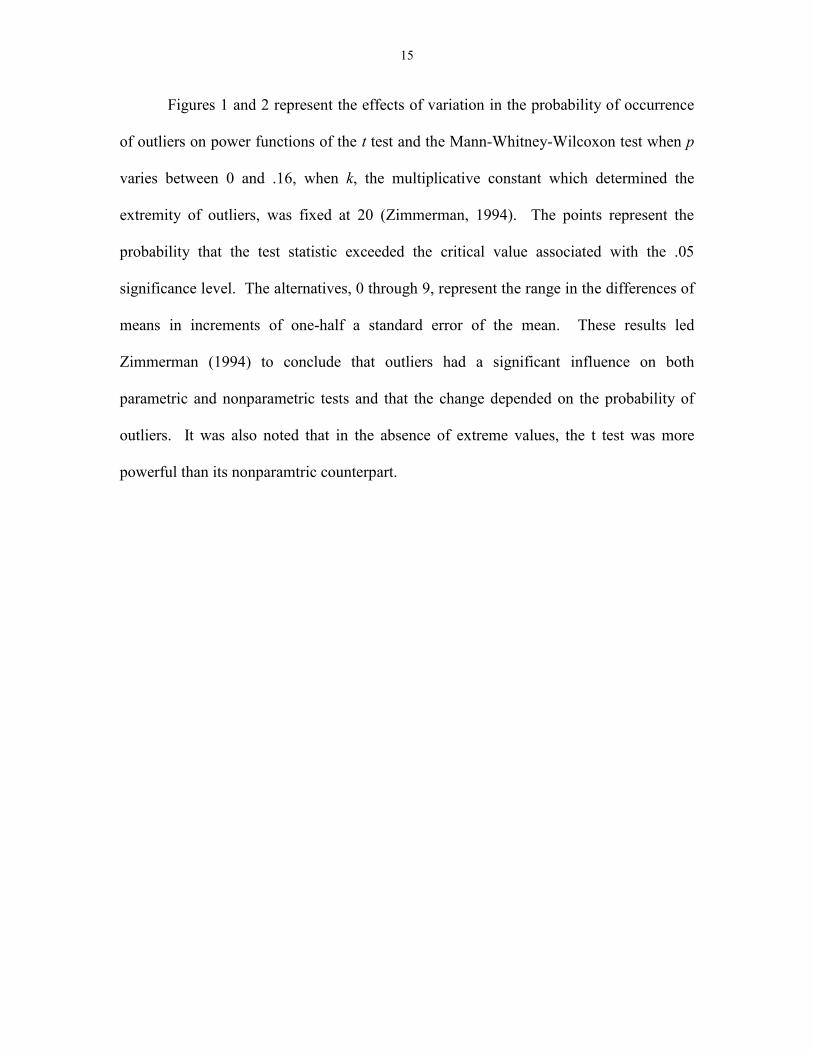
Figure 2. Effects of variations in the probability of occurrence of
an outlier on power functions of the Mann-Whitney-Wilcoxon test,
Zimmerman (1994)
15
Figures 1 and 2 represent the effects of variation in the probability of occurrence
of outliers on power functions of the t test and the Mann-Whitney-Wilcoxon test when p
varies between 0 and .16, when k, the multiplicative constant which determined the
extremity of outliers, was fixed at 20 (Zimmerman, 1994). The points represent the
probability that the test statistic exceeded the critical value associated with the .05
significance level. The alternatives, 0 through 9, represent the range in the differences of
means in increments of one-half a standard error of the mean. These results led
Zimmerman (1994) to conclude that outliers had a significant influence on both
parametric and nonparametric tests and that the change depended on the probability of
outliers. It was also noted that in the absence of extreme values, the t test was more
powerful than its nonparamtric counterpart.

16
Figure 3. Probability of Type I errors of the Student’s t test
when the null hypothesis is true, Zimmerman (1994).
Figure 4. Probability of Type I errors of the Mann-Whitney-
Wilcoxon test when the null hypothesis is true, Zimmerman
(1994).
17
Figures 3 and 4 depicts the effect of variation in the extremity of outliers on
power functions on Student’s t test and the Mann-Whitney-Wilcoxon test when p was
held at 0.05 and k was allowed to vary between 1 and 40. The variations in k caused the t
test to variation slightly, however the Mann-Whitney-Wilcoxon test remained constant.
Zimmerman (1994) concluded from this, that the decline in probability
depended jointly on k and p for the parametric test, however the nonparametric test was
only sensitive to the affects of p ( p. 395). In addition, Zimmerman’s findings suggest
correction on previously held positions that Type II errors and the power of some
nonparametric methods are not affected by the underlying shape of a distribution. On the
contrary, this reserach suggests that outliers affect both nonparametric and parametric
tests, especially when samples are drawn from the mixed-normal distribution.
Nonparametric tests, however, prove to be more robust under these conditions
(Zimmerman 1994, p. 397).
Lindquist (1953), on the other hand, held strong to convictions that parametric
procedures were far superior to their nonparametric counterparts. To prove the
robustness under non-normality of a classic parametric estimator, the F test, Lindquist
described a study conducted by his student Norton, in which six different distributions
(normal, leptokurtic, rectangular, moderately skewed, markedly skewed and j-shaped)
were investigated. These distributions were representative of those found in education
and psychology studies. Distributions having the same criterion measures were studied
in four different phases where various types of assumption violations were considered
through the construction of card populations based on 10,000 cases each. The resulting
18
distributions were then compared against the normal population for the F distribution.
The findings of the experiment led Lindquist (1953) to conclude the following:
The results of the Norton study should be gratifying to anyone who has used or
who contemplates using the F test of analysis of variance in experimental
situations in which there is serious doubt about the underlying assumptions of
normality and homogeneity of variance. Apparently, in the great majority of
situations, one need be concerned hardly at all about lack of symmetry in the
distribution of criterion measures, so long as the distribution is homogenous in
both form and variance for the various treatment populations, and so long as it is
neither markedly skewed nor markedly flat…In general, the F distribution seems
so insensitive to the form of the distribution of criterion measure that it hardly
seems worthwhile to apply any statistical test to the data to detect non-normality,
even though such tests are available. Unless the departure from normality is so
extreme that it may be easily detected by mere inspection of the data, the
departure from normality will probably have no appreciable effect on the validity
of the F test, and the probabilities read from the F table may be used as close
approximations to the true probabilities. (p. 86)
Conclusions reached by Norton (1952) and Lindquist (1953) alike served as the
foundation for the continued implementation of parametric procedures, as well as paved
the way for parametric robustness studies later conducted by Boneau (1960) and Glass,
Peckham and Sanders (1972).
A large part of Boneau’s study (1960, 1962) was dedicated to demonstrating that
violating assumptions, particularly normality, when using the t test or F test, does not

19
have an effect on the test’s ability to maintain its robustness in terms of Type I error for
departures from population normality (p.1). To prove his argument, Boneau (1960)
computed a large number of t values based on randomly drawn samples from
distributions (normal, exponential (J-shaped with a skew to the right), and rectangular or
uniform) having specified characteristics. Frequency distributions of obtained t values
were constructed and superimposed over the normal distribution for comparison. Based
on his findings, Boneau (1960) concluded that “violating assumptions, particularly
normality, produced minimal effects on the distribution of t’s and that the t test was an
essentially robust test in the technical sense of the word” (p.61). Boneau (1960) further
asserted that:
The t test could hold its robustness against violations of homogeneity of variance
and normality as long as: (a) the two samples were equal or nearly so; and (b) the
assumed underlying population distributions were of the same shape or nearly
so…If these conditions are met, then no matter what the variance differences may
be, samples of as small as five will produce results for which the true probability
of rejecting the null hypothesis at the .05 level will more than likely be within .03
of that level…the percentage of times the null hypothesis will be rejected when it
is actually true will tend to be between 4% and 6% when the nominal value is 5%
(p.62)…however in situations where a combination of unequal sample size and
unequal variances exists, there is a risk of inaccurate probability statements being
produced, which would differ significantly from the nominal values…In these
situations, alternative testing procedures such as those suggested by Cochran and

20
Cox (1950), Sattertwaite (1946), and Welch (1947) would be more feasible.
(p.62).
In a follow-up study, Boneau (1962) expounded on his previous work to compare
the power of the nonparametric U test against its parametric competitor the t test, to
determine the probabilities of rejecting the null hypothesis if it was true. Using methods
similar to those implemented in his previous study, comparisons of the power of the two
tests were made under the following assumption: normal distribution with homogenous
variance, normal distribution with heterogeneous variance and non-normal distribution.
From this study, Boneau (1962) concluded:
…that for normal distributions with homogenous variance, the t test was the
uniformly most powerful test; however its margin over the U test was very slight.
Points at which the U test showed superiority over the t test must have been due to
sampling error because of the power property of the t test under these conditions.
Under the normal distribution with heterogeneous variance, the t test seemed to be
relatively unaffected by the homogeneity violation, as well as the U test; however,
the U test was still slightly less powerful than the t test in this situation. (p.250).
Boneau (1962) further noted that “when sampling took place from at least one
non-normal distribution, in this case the rectangular distribution, the power of the t test
was quite greater than that of the U test, but never by much except at the .01 level”
(p.253). For the exponential distribution with small differences between means, the U
test held power superiority over the t test, but as mean differences increased, this
advantage disappeared. For the non-normal distributions, it was concluded overall that
“when distributions had the same shape outside of normality, the power functions of the t

21
and U tests had a relatively constant relationship, where the t was more powerful than the
U in most cases” (Boneau, 1962, p.254).
In an attempt to further validate the theory of parametric robustness, Glass et al.
(1972) examined the consequences of failing to meet the assumptions underlying the
fixed effects ANOVA. In their study, Glass et al. (1972) asserted that “the relevant
question was not whether ANOVA assumptions were met exactly, but whether the
plausible violations of the assumptions of the ANOVA had serious consequences on the
validity of probability statements based on the standard assumptions” (p. 237).
Violations of non-independence of errors, non-normality (skewness, kurtosis and
heterogeneous variances), and combined non-normality and heterogeneous variances of
the fixed-effects ANOVA were discussed, along with the effects on α for both equal and
unequal n’s.
(1952), Lindquist (1953), and Boneau (1960), Glass et. al (1972) proposed the following
conclusions about the consequences of violating the assumptions of the fixed-effects
ANOVA and the effects that it had on α:
1. Non-independence of errors seriously affected the level of significance of the
F test regardless of whether n’s are equal or unequal;
2. Skewness had a minimal effect on the level of significance of the fixed-effects
model F test and distortions of nominal significance levels of power values
were rarely greater than a few hundredths (however, in the case of the one
tailed or directional test, skewness can have serious implications on the level
of significance);

22
3. In reference to kurtosis for both equal and unequal n’s, the actual α was less
than the nominal α for leptokurtic populations. However, for platykurtic
populations actual α exceeded nominal α;
4. For heterogeneous variances and equal n’s, the effects on α were slight, with
distortions of no more than a few hundredths; actual α was always slightly
elevated over nominal α. For unequal n’s, actual α exceeded nominal α when
smaller samples were drawn from more variable populations; actual α was
also less than nominal α when smaller samples were drawn from less variable
populations; and
5. In the case where a combination of non-normality and heterogeneous
variances existed, the two appeared to combine additively to affect either level
of significance or power (Glass et. al., 1972, p.273).
In rebuttal to claims of robustness of the t and F tests under violations of
assumptions, particularly non-normality, Blair (1981) argued that “previously held
positions by Boneau (1960, 1962), Glass et al. (1972) and others should be avoided,
particularly when sampling from non-normal distributions” (p. 499). Glass et
al.continued to argue that the asymptotic relative efficiency (A.R.E) or Pitman efficiency
of the two sample t test was .955 under normality and homogeneity when compared with
the Wilcoxon rank-sum test (Blair, 1981, p. 500). Blair (1981), however, refuted this
argument stating that it “encouraged further exaltation of the superiority of the t test over
its nonparametric competitors, even under non-normal situations” (p.500) and that Glass
et al. erred in their conclusions because they failed to consider the following criteria:

23
1. The Type I error issue was only a necessary, rather than a sufficient
condition for the position they took, because it did not take into account
the usefulness of nonparametric counterparts of the t test;
2. The relative power of the t test and its nonparametric counterparts under
varying population shapes;
3. In situations where the t test was more powerful than the Wilcoxon test,
the magnitude of the advantage was modest;
4. Statistical theory and empirical demonstration indicated that the
Wilcoxon statistic enjoys very large power advantages over the t test;
and
5. Educational data are often distributed in a radically non-normal manner
(p.506)
Blair et al. (1980) also countered Boneau's (1960, 1962) position on the
comparative power of the t test against that of the U test in applied research settings. In a
challenge to Boneau’s former study, computer simulation techniques were implemented
to re-examine a portion of work previously conducted to determine if Boneau had erred
in his conclusions about the alleged power advantage of the t test over the U test. Using
the exponential population and 1,000 samples, Blair et al. (1980) utilized a wider range of
sample sizes and consistent alpha levels to conduct their study.
Blair et al. (1980) determined that Boneau (1962) “erred in concluding that in
applied situations, the Mann-Whitney U test did not demonstrate the power advantages
that are potentially associated with this statistic according to statistical
theory”(p.118). The study cited that one probable cause of Boneau’s error was his

24
application of the U test on small sample sizes and the fact that the U test performs rather
poorly with small sample sizes (Blair et al.,1980).
Sawilowsky and Blair (1992) also recognized the power of the Wilcoxon rank-
sum test when testing for shifts in location parameter (p.359). In a Monte Carlo
comparison of the power of the independent samples t test and the Wilcoxon rank-sum
test, samples of size (5,15) were drawn from the extreme asymmetric distribution at α =
.05 and ES of .2. Findings indicated the power of the Wilcoxon test was .395, compared
with .139 for the t test and when the ES was increased to .5, the power of the Wilcoxon
test measured .723, while the t test was found to be .495 (Sawilowsky & Blair, 1992,
p.359).
In another case, Blair and Higgins (1981) argued against the relative efficiency of
the t test versus nonparametric alternatives, such as the Wilcoxon rank sum test. In this
study, a comparison was made of the relative efficiency of the parametric t test against
the nonparametric Wilcoxon rank sum statistic to test for shift in two-sample cases (Blair
and Higgins, 1981). Various mixed normal distributions were tested based on theoretical
considerations and because mixed normal distributions have been shown to be
appropriate models for variables occurring in a wide variety of disciplines (Blair &
Higgins, 1981, p.124). Results of this study seemed to contradict Boneau’s former
research.
Two Sample T Test
It is a well argued fact that the two sample independent t test is one of the best
known statistical procedures in current use when applied under normal conditions. This a
major cause for concern because this test is often applied in both normal and non-normal

25
conditions, which makes violating the normality assumption an even greater concern.
Sawilowsky and Blair (1992) noted, however, that for the test to be considered robust
under assumption violations, insofar as Type I errors were concerned to non-Gaussian
populations, certain stipulations had to be met :
(a) sample sizes had to be equal or nearly so;
(b) sample sizes were fairly large; and
(c) tests were two-tailed rather than one-tailed (Sawilowsky & Blair, 1992, p.352)
Under these conditions, if differences were found to exist between nominal alpha
and actual alpha levels, Sawilowsky and Blair (1992), in referencing other sources (see
e.g., Efron, 1969; Gayen, 1949, 1950; Geary, 1936, 1947; Pearson & Please, 1975)
contended that “the discrepancies were usually of a conservative rather than a liberal
nature” (p. 352). Bradley (1980), however, objected the claim that the t test was robust
under conditions of nonnormality because the term “large” could not be adequately
quantified and because many distributions encountered in real-world situations were
more non-normal than those referenced in robustness studies (Bradley, 1968; 1977;
1982).
Sawilowsky and Blair (1992) also conducted Monte Carlo experiments on eight
real distributions previously studied by Micerri to determine the robustness of the two
independent samples t test with respect to departures from population normality.
Independent samples comprised of sizes (n1, n2) = (5,15), (10,10), (10,30), (20,20),
(15,45), (30,30), (20,60), (40,40), (30,90), and (60,60) were sampled with replacement
with the independent samples t test computed on each pair of samples (Sawilowsky &
Blair, 1992, p.353). Based on conclusions from this study, Sawilowsky and Blair (1992)

26
noted:
The distributions studied provided a more realistic and stringent test of the t test’s
sensitivity to population shape than has been afforded by previous studies on this
topic. These real distributions highlight situations in which the t test was, by
definition, nonrobust to Type I error. The degree of nonrobustness seen in
instances was at times more severe than has been previously reported. (p. 359).
In addition, it was maintained that “when the normality assumption is violated,
the mean and variance, (parameters used to estimate the t test), are inexact “(Micerri
1986, 1989). Micerri (1986) further argued that:
As a point estimator of location in the presence of non-normality, the mean has
not proven relatively robust when estimating the center of symmetry in heavy-
tailed symmetrical distributions (Andrews, Bickel, Hample, Huber, Rogers and
Tukey, 1972), in the presence of a single outlier (David and Shu, 1978), in the
presence of serially dependent data (Gastwirth and Rubin, 1975; Wegman and
Carroll, 1977), in the presence of asymmetric data (Jaeckel, 1971; Ansell, 1973;
Carroll, 1979; Kimber, 1983, or finally in the presence of specific “real” data
(Stigler, 1977; Tapia and Thompson, 1978; Hill and Dixon, 1982) (p.2)
These findings reiterated points stressed in earlier research (Sawilowsky and
Blair,1992; Wilcox, 1996; Micerri, 1989) of how relatively minute departures from
normality can cause tests such as the t, F or ANOVA to be inexact.
Trimmed and Winsorized Means
As a proposed alternative for implementing the two sample t test under
nonnormality, several theorists (i.e., Tukey & McLaughlin, 1963; Yuen, 1974; Hogg

27
,1974; Stigler, 1977; Cressie, 1980; Hill & Dixon, 1982) recommended applying trimmed
means for dealing with distributions whose standard errors were affected by the presence
of outliers or heavy-tailedness or for improving control over Type I error inflations.
Yuen’s (1974) study investigated the effects of Welch’s approximate degrees of freedom
t test and the trimmed t test under unequal variance for both the normal and long-tailed
distributions. Using a Monte Carlo simulation, Type I error probabilities were obtained
for Cauchy, normal, uniform, Student’s t, and mixed uniform/normal distributions for
samples sizes of 10 to 20 with nominal sizes 0.01, 0.05, and 0.10 for 5,000 samples with
10,000 iterations (Yuen, 1974). Results led Yuen (1974) to conclude that deviations for
Welch’s test were greater than that for the trimmed t test, meaning that the trimmed t had
a greater probability of rejecting the null hypothesis when it was actually true. Power
results also indicated that the trimmed t never exceeded the power Student’s t under exact
normality and that small amounts of trimming had minimal affects on the loss of power.
It also appeared that degree of tail length, level of trimming, and sample size caused the
trimmed t to hold superior power advantages over Welch’s test.
Several authors (Kesselman et. al, 2004; Fisher, 1935; Brown & Forsythe, 1974;
Wilcox, 1990) have argued that the when conducting statistical investigations using the
two sample t test, the test is highly unstable in the presence of nonnormality and
heteroscedasticity. When estimating the mean, some researchers (Dixon, 1960; Tukey &
McLaughlin,1963; Dixon & Tukey,1968) have suggested feasibility of implementing
some form of adaptive robust procedure, particularly when it is suspected that some
individuals in the sample may have come from a population other than the population
being studied of interest. Techniques such as trimming and winsorizing have been

28
proposed as ways to minimize the effects of long tailed distributions, which have been
known to be the cause of outliers.
The concept of winsorizing data was first suggested by Charles Winsor (1940)
and later renamed by Tukey (1962) as the winsorized mean (Fuller, 1991). Rivest (1994)
suggested implementing the winsorized mean because of its simplicity and efficiency in
reducing the impact of the largest observations. Dixon (1960) suggested that the
efficiency of the symmetrically winsorized mean for location under normality is quite
high, particularly when compared to the most efficient linear combination of the same
order statistic (Dixon & Tukey, 1968, p. 83).
While trimming data has often been a highly practiced technique, especially when
the data are heavy-tailed, many practitioners shun the practice because trimming removes
data values which may or may not affect the significance of statistical results. The
winsorized mean, unlike the trimmed mean however, preserves the original observations
in the data set by pulling outliers towards the middle of the distribution. The general
form of winsorization replaces the largest r observations by the (r + 1)st largest
observation and replaces the s smallest observations by the (s + 1)st smallest (Fuller,
1991, p. 138). Bennett (2009) demonstrated calculation of the winsorized mean using the
following data set, 25, 55, 11, 24, 22, 21, 13, 42, 25, 22. First, the observations are
ordered from least to greatest, 11, 13, 21, 22, 22, 24, 25, 25, 42, 55, and the number of
observations to winsorize calculated using the formula, g =.2 • n, where n represents the
sample size and g equals the number of observations winsorized from each side. In this
case, two observations were recoded on each side of the winsorized sample, 21, 21, 21,
22, 22, 24, 25, 25, 25, 25, which equates to 20% winsorization. The winsorized mean,

29
x_
w, is then calculated by summing the observations and dividing by n, in this case x_
w =
23.1. Dixon and Massey (1969) argued that if the smallest and largest observations are
given the value of their nearest neighbor, a technique referred to as first-level
winsorization, the computed mean of the modified sample will not have lost much
efficiency if the extremes are actually valid (p. 330).
In an attempt to prove the effectiveness of the winsorized mean on heavy-tailed
distributions, Fuller (1991) explored the effects of the once-winsorized mean on the
Weibull distribution. The Weibull distribution is a right skewed distribution that is a
highly used in reliability and life data analysis due to its versatility and ability to model a
number of real life behaviors. Fuller (1991) argued that investigation of the Weibull
distribution is beneficial to the practice of statistics because many empirical distributions
have tails which resemble the Weibull (p.139). In the study, the mean square error was
used as the criterion to prove that the once-winsorized mean is superior to the sample
mean for the Weibull when the shape parameter is greater than one, has the same
efficiency as the mean if equal to one, and is less efficient than the mean if less than one
(Fuller, 1991, p.139). In concluding the study, Fuller (1991) referenced McElhone’s
(1970) table of efficiencies of estimators relative to the mean for the Weibull distribution,
noting that large gains in efficiency when using the once-winsorized mean. In addition,
for a Weibull with shape parameter γ = 2 and sample size n = 25, the winsorized mean
was 24% more efficient than the mean; for n = 25 and γ = 3, the winsorized mean was
twice as efficient as the sample mean; and for n = 25 and γ = 3, the winsorized mean was
more than four times as efficient as the sample mean (Fuller, 1991, 144). Fuller (1991)
further noted that in instances when r > 1, the mean was uniformly more superior than the

30
winsorized mean on the basis of mean square error, however little difference was
detected among the mean square errors with reasonable sample sizes (n > 4) for all three
estimators. These findings led Fuller to conclude that the once-winsorized mean is
superior to the mean for the Weibull distribution with parameter γ > 1 (Fuller, 1991, 146).
Figure 5.Weibull Distribution
(http://www.engineeredsoftware.com)
Rivest (1994) also suggested winsorizing as a strategy for improving the sample
mean, which for the exponential distribution, can significantly reduce the mean squared
error of the sample mean by an O(1/n2) term. Efficiency and bias comparisons of the
winsorized mean were examined via Monte Carlo approximations and exact calculations
for sample sizes varying between 20 and 200 from the Weibull, lognormal, and Pareto
distributions with coefficients of variation 2 and 4 (Rivest, 1994, p.378). For the two
Weibull distributions, as well as the lognormal, where β = 1.27, it was found that

31
winsorizing less than one observation helped maintain efficiency, while significantly
reducing bias (Rivest, 1994, p.378). The study concluded overall that winsorized means
are an efficient alternative to the sample mean, especially for populations that are
skewed, and that even in the presence of heavy skewness, the once-winsorized mean 1
provides the largest efficiency, whereas the 0.75 mean is better suited for less moderate
skewness (Rivest, 1994).
Winsorization techniques have also been shown to play a critical role in
alleviating power issues. The two sample winsorized t test is given by the formula:
_ _
1 2
2 2
2 1 2 2
1 2
1 2
1 1( 1) ( 1)
2
w ww
x xt
n s n s n nn n
where the Winsorized sum of squared deviations is calculated using the formula:
22 21_ _
2
( )( 1) ( )
2
_1 1
n k
wk i wkwk k n ki k wk
k y y k yy ys y
Dixon and Massey (1969) noted that winsorization techniques can also be applied
in cases where data are missing or omitted in equal number at either extreme. In cases
such as these, efficiency estimates are approximated at 99.9 % when compared to the best
possible linear estimate based on these same observations for samples from normal
populations with sample sizes 20 or less (Dixon, 1960). In the table below, derived from

32
Dixon and Massey (1969), efficiencies for various levels of trimming and Winsorizing
are compared:
Table 1. Efficiencies for trimmed and winsorized samples.
It is obvious that Dixon and Massey’s (1969) argument that winsorization is
superior to trimming is valid. In cases where the symmetrically placed extreme
observations are trimmed as opposed to winsorized, the arithmetic mean of the remaining
observations provided as estimate of smaller efficiency (Dixon and Massey, 1969, p.
331).
Micerri (1989) also noted that 97% of all empirical distributions studied in
psychology and education had longer tails than the normal distribution, with the
remaining 3% having an approximately normal distribution. Sawilowsky and Blair
(1992) argued that in cases where the normality of the underlying distribution was in
question, the t test would only yield valid results if sample sizes were greater than 30 per
group, the groups had equal sample sizes and the test being conducted was two-tailed
rather than one-tailed. However if those conditions were unmet, which they rarely are in
empirical studies, validation of statistical results would be questionable.
Fung and Rahman (1980) recommended the winsorized t be used in situations
when the underlying distribution is long-tailed. Often times, however, researchers are not
N Trim. Wins. Trim. Wins. Trim. Wins. Trim. Wins.
10 .949 .958 .883 .889 .808 .821 .723 .723
20 .978 .984 .948 .962 .915 .936 .880 .905
k = 1 k = 2 k = 3 k = 4

33
aware of the shape of the underlying distribution prior to implementing statistical
analysis. Since the results of this study demonstrate that the distribution of the
winsorized t test approximates Student’s t distribution, more consideration should be
given towards implementing nonparametric statistical procedures, such as the winsorized
t test because of its robustness against concerns of nonnormality. Implementing
nonparametric procedures such as the winsorized t test may prove to be invaluable for
drawing valid statistical inferences, as well as helping to maintain nominal Type I error
probabilities.
Monte Carlo Methods
Monte Carlo methods refer to a class of mathematical computations which rely on
repeated random sampling to determine results to make inferences about the population
from which a sample has been drawn. The term was also used by Sawilowsky and
Fahoome (2003), to refer to methods that describe repeatedly sampling from an identified
probability distribution to determine the long run average of a specific parameter or
characteristic. This method relies on sampling with replacement, meaning that when a
subset of scores has been selected, recorded and analyzed, they are returned to the
sampling distribution. The process is then repeated many times with the likelihood of the
scores previously chosen having the same probability of being chosen again as values not
previously selected. Monte Carlo Methods were first introduced in the early 1930’s by
physicist Enrico Fermi and later adopted and improved by John von Neumann and
Stanislaw Ulam for simulations of the atomic bomb during the Manhattan Project. There
are several classes of Monte Carlo Methods, including Monte Carlo estimation,

34
bootstrapping, the jackknife, and Markov Chain Monte Carlo estimation, however this
study will focus solely on Monte Carlo Estimation.
Bernard was the first to implement Monte Carlo Estimation in 1963 to test the
hypothesis that data represented a random sample from a specified population (Noreen,
1989; Kelly, 1999). Noreen (1989) added that Monte Carlo estimation is best utilized in
situations where the population is known, but the sampling distribution has not yet been
derived. Sawilowsky and Fahoome (2003) noted that Monte Carlo simulations rely on
computer models and are particularly useful because the quality of the simulation
increases as the model increases its ability to mimic reality. To conduct Monte Carlo
estimations, the following steps are conducted:
1. A matrix of artificial data is generated which matches the assumptions of the
analysis and for which the null hypothesis is true.
2. The value of the test statistic of interest is computed for each sample.
3. The computed simulated sample statistics are then ordered in a distribution, called
the "Monte Carlo distribution" of the statistic.
4. The "real" statistic is then mapped onto the Monte Carlo distribution using the
would-be percentile rank of the "real" statistic to identify the 5%, 2.5%, 1% and
0.5% critical values.

35
CHAPTER 3
METHODOLOGY
Overview
To approximate the distribution of the winsorized t test in an effort to generate a
table of critical values for the two sample winsorized t test, a program was written in
Excel using Visual Basic with Applications programming language. First, the code for
the two sample winsorized t test function was written and tested on real data with 0%
winsorization to determine the accuracy of the algorithm. The results of testing the data
with the winsorized algorithm were then compared to the results of the traditional two
sample t test. Both functions yielded a t score equivalent to t = 0.41597, which verified
the veracity of the winsorization algorithm. The algorithm was then used to winsorize a
user specified number of observations from both sides of the data, in this case one and
two values from both tails were recoded, equating to a 10% and 20% winsorization. The
data was computed again using the winsorized t test algorithm, yielding a winsorized t
score of = 0.27681 for 10% winsorization, and -0.53045 for 20% winsorization.

36
Table 2. Sample data used to verify algorithm
The program was then modified to sample random data from Excel’s normal
distribution, NORMINV, with μ = 0 and σ = 1. First, an algorithm was written to
calculate both the winsorized mean and winsorized sample variance for both samples A
and B. The winsorized sample variance was then used to calculate the pooled winsorized
sample variance having n1+ n2 -2 degrees of freedom. The winsorized mean and pooled
sample variance were then fed to a subroutine that was used to calculate the two sample
winsorized t test. The results of the test statistic were then stored in an array or matrix
and the procedure reiterated until 1,000,000 repetitions were completed. Each winsorized
t score was then sorted from low to high (t1, t2, t3,…t 1,000,000) in an effort to identify the
critical values at the 95th
, 97.5th
, 99th
and 99.5th
percentiles. These values represent the
critical values for both one and two tailed tests for α = 0.05 and 0.01. The results were
then arranged in a table according to the formula n1 + n2 – 2, which represents the
degrees of freedom for the two sample winsorized t test. To test the accuracy of this
SAMPLE A SAMPLE B -1.39 -1.28 -1.22 -1.08 -1.01 -0.87 -0.77 -0.22 -0.34 -0.01 0.44 0.35 0.74 0.92 0.88 1.10 2.80 1.21 4.10 1.39

37
subroutine, a Monte Carlo simulation was run using random samples with winsorization
equivalent to 0% for sample size n1 = n2 =2. Random samples were drawn, with
replacement, from the normal population and the procedure reiterated 1,000,000 times.
Results were then sorted, ranked and the corresponding percentiles identified for both
samples A and B. The critical values representing the 95th
, 97.5th
, 99th
and 99.5th
percentiles for both one and two-tailed tests were then compared to the critical values
produced by Student’s t table and the percentage of error calculated to determine the
accuracy of the subroutine. Table 3 below compares the results of the 0% winsorized
Monte Carlo simulation and Student’s t test critical values for sample size n1 = n2 =2.
Results from the simulation illustrate that the subroutine provided valid results for
approximating the distribution of the Student’s t distribution and that the margin of error
between the two is minimal.
Table 3. Monte Carlo summary results for sample size n1= n2 =2.
POPULATION TYPE
Normal Random Dist.
SAMPLE SIZE A
2
SAMPLE SIZE B
2
WINSORIZATION A
0 Per Side
WINSORIZATION B
0 Per Side
ACTUAL WINSORIZED PERCENT A 0%
ACTUAL WINSORIZED PERCENT B 0%
DEGREES OF FREEDOM 2
ITERATIONS
1000000
Conf. 1-Tail p 2-Tail p C.V. abs error error %
90.00% 0.05 0.1 2.91982 0.00017 0.005832%
95.00% 0.025 0.05 4.30756 0.00491 0.114101%
98.00% 0.01 0.02 6.97036 0.00581 0.083393%
99.00% 0.005 0.01 9.94828 0.02344 0.236175%

38
Sample sizes equivalent to n1 = n2 = 5 to 30, 45, 60, 90 and 120 were then drawn
from the normal population and symmetrically winsorized or recoded, up to 20%, where
r observations were recoded on each side of the data. Table 4 illustrates the experimental
sample sizes and the number of observations that were winsorized on each side for each
sample size.
Table 4. Maximum winsorized values per side for the two sample winsorized t.
_______________________________________________________
Sample Size Maximum number of observations
Winsorized per side
_______________________________________________________
5-9 1
10-14 2
15-19 3
20-24 4
25-29 5
30 6
45 9
60 12
90 18
120 24 __________________________________________________
Computer Hardware and Software
All of the programs, functions and subroutines generated in Excel were developed
using an HP Intel (R) Core ™ 2 CPU T7200 notebook with an AMD Athlon(tm) 64
processor and 2.00 GHz of memory and 2.49 GB of RAM memory. The hardware was
supported by the Microsoft Windows XP Tablet PC 2005 Edition operating system with
Service Pack 3. Microsoft Visual Basic version 6.5 was utilized to write and execute

39
programs, generate random samples and calculate the specified test statistic. Monte
Carlo Simulations of all sample sizes were performed at Wayne State University’s
College of Education Computer Lab using 30 Apple Dual-Boot Computers with Intel ®
core ™ with 2.66 GHz memory and 2.98 GB of RAM. The computers were supported
by Microsoft Windows XP Professional version 2002 operating system with service pack
3.

40
CHAPTER 4
RESULTS
Synopsis
A Monte Carlo experiment was designed to approximate the distribution of the
two sample winsorized t test. Samples were drawn from Excel’s normal distribution with
μ = 0 and σ = 1 for sample sizes n1 = n2 = 5 to 30, 45, 60, 90 and 120. For each pair of
samples, the winsorized t statistic was calculated 1,000,000 times on various levels of
winsorization up to 20%. The values were then ranked from low to high and the values at
the 95th
, 97.5th
, 99th
and 99.5th
percentiles identified, which represented the critical values
for both one and two-tailed tests at α = 0.01 and 0.05. Finally, the distribution of the two
sample winsorized t was examined to determine its approximate behavior as sample sizes
increased.
Winsorized Trials
For sample sizes n = 5 through 9 and df = 8 to 16, one observation was
symmetrically winsorized from both sides of the sample in order not to exceed
winsorization levels of more than 20%, and to maintain an unwinsorized core of at least
n = 2. When the critical values were examined in comparison to Student’s t distribution,
results showed that the values for the winsorized t distribution were 2.2 to 2.8 times
greater than those of Student’s t distribution. For example, for df = 8 at the 99.5th
percentile, the critical value for the winsorized t distribution was 9.3822, whereas the
value for Student’s t distribution was 3.355. These findings are significant, because
according to Fung and Rahman (1980), in the past researchers have used Student’s t
distribution to approximate the distribution of the winsorized t using h1 + h2 -2, where h

41
represented the number of unwinsorized observations. When testing hypotheses of the
differences between means, the null hypothesis, Ho, is rejected if |T| > t1-α/2 for two tailed
tests and T > t1-α and T < tα for one tailed tests. For example, for a calculated T = 2.883
for α = 0.05 and df = 8, using Student’s t distribution, the null hypothesis would be
rejected for both the two sided and right tailed tests. On the other hand, if the same
results are compared against the winsorized t distribution, the researcher would fail to
reject the null hypothesis for both right and two-tailed tests only. This dilemma can
certainly have a negative impact on the interpretation statistical results, as well as impede
researchers’ ability to draw definitive inferences about the effectiveness of their research.
When samples sizes were incremented and more than one observation was
winsorized from each side, results showed that in every case, the once winsorized
samples provided more nominal critical value levels than samples with more observations
winsorized on each side. It was also observed that as degrees of freedom increased, the
critical values for the winsorized t distribution also began to decrease. However, as the
critical values began to decrease, only first level winsorization showed any close
approximation to Student’s t values. This illustrates that first level winsorization, or
recoding of one value from each side of a sample, provides critical value approximations
which are closer to those of Student’s t distribution.
Critical values for subsequent levels of winsorization can also prove useful. As
the number of observations symmetrically winsorized increases, the better the winsorized
mean approximates the median. As proven by previous research, the median is a measure
of central tendency which is resistant to the effects of outliers. Therefore, the more
observations winsorized, the lesser the impact of outliers and heavy-tailedness on the

42
mean and variance. While first level winsorization may prove to be more effective in
cases of mild departures from normality, more severe cases may be better served by
increasing the number of symmetrically winsorized observations. According to Tukey
and Dixon (1968) there is no predetermined threshold of winsorization that has proven to
be more effective, however, the authors did provide winsorized critical values for various
sample sizes, leaving winsorization levels to the discretion of the researcher.

43
Table 5. Critical values for the two sample winsorized t test
1-tailed 0.05 0.025 0.01 0.005
2-tailed 0.1 0.05 0.02 0.01
df (ν)
R # Winsorized
Per Side
Sample
Size
8 4.0844 5.4216 7.4907 9.3822 1 5
10 3.1400 4.0019 5.2148 6.1936 1 6
12 2.7239 3.4014 4.3188 5.0422 1 7
14 2.4813 3.0736 3.8391 4.4223 1 8
16 2.3368 2.8613 3.5373 4.0538 1 9
18 2.2268 2.7197 3.3414 3.8090 1 10
18 3.1680 3.9250 4.9310 5.7130 2 10
20 2.1545 2.6204 3.2051 3.6385 1 11
20 2.8913 3.5590 4.4199 5.0690 2 11
22 2.0950 2.5422 3.0944 3.4948 1 12
22 2.7071 3.3137 4.0845 4.6552 2 12
24 2.0484 2.4786 3.0088 3.3974 1 13
24 2.5658 3.1255 3.8286 4.3598 2 13
26 2.0090 2.4311 2.9396 3.3045 1 14
26 2.4543 2.9875 3.6427 4.1156 2 14
28 1.9803 2.3912 2.8863 3.2440 1 15
28 2.3734 2.8726 3.4930 3.9484 2 15
28 2.9765 3.6351 4.4560 5.0747 3 15
30 1.9521 2.3528 2.8384 3.1900 1 16
30 2.3029 2.7846 3.3830 3.8116 2 16
30 2.8216 3.4284 4.1941 4.7568 3 16
32 1.9289 2.3243 2.8023 3.1377 1 17
32 2.2444 2.7145 3.2854 3.6941 2 17
32 2.7013 3.2756 3.9880 4.5066 3 17
34 1.9099 2.3000 2.7699 3.0952 1 18
34 2.2001 2.6549 3.2044 3.5932 2 18

44
Table 5 (con’t). Critical values for the two sample winsorized t test
1-tailed 0.05 0.025 0.01 0.005
2-tailed 0.1 0.05 0.02 0.01
df (ν)
# Winsorized
Per side
Sample
Size
34 2.5994 3.1490 3.8203 4.3063 3 18
36 1.8920 2.2758 2.7362 3.0648 1 19
36 2.1573 2.5983 3.1358 3.5182 2 19
36 2.5144 3.0430 3.6938 4.1605 3 19
38 1.8741 2.2546 2.7133 3.0355 1 20
38 2.1181 2.5529 3.0820 3.4523 2 20
38 2.4412 2.9493 3.5728 4.0194 3 20
38 2.8915 3.5056 4.2682 4.8220 4 20
40 1.8651 2.2409 2.6920 3.0111 1 21
40 2.0882 2.5175 3.0262 3.3954 2 21
40 2.3867 2.8846 3.4781 3.9135 3 21
40 2.7877 3.3776 4.0932 4.6048 4 21
42 1.8496 2.2227 2.6658 2.9739 1 22
42 2.0636 2.4809 2.9816 3.3381 2 22
42 2.3315 2.8108 3.3885 3.8017 3 22
42 2.6930 3.2559 3.9307 4.4257 4 22
44 1.8392 2.2100 2.6488 2.9589 1 23
44 2.0375 2.4491 2.9421 3.2910 2 23
44 2.2881 2.7561 3.3162 3.7232 3 23
44 2.6133 3.1564 3.8220 4.2893 4 23
46 1.8303 2.1975 2.6366 2.9425 1 24
46 2.0195 2.4253 2.9139 3.2572 2 24
46 2.2488 2.7074 3.2608 3.6484 3 24
46 2.5463 3.0739 3.7151 4.1677 4 24
48 1.8226 2.1864 2.6228 2.9306 1 25
48 1.9972 2.3992 2.8851 3.2255 2 25
48 2.2157 2.6657 3.2119 3.5880 3 25
48 2.4890 2.9986 3.6248 4.0610 4 25
48 2.8465 3.4415 4.1657 4.6849 5 25
50 1.8159 2.1745 2.6065 2.9057 1 26
50 1.9801 2.3746 2.8487 3.1775 2 26
50 2.1855 2.6259 3.1519 3.5193 3 26
50 2.4382 2.9347 3.5395 3.9573 4 26
50 2.7688 3.3367 4.0308 4.5286 5 26
52 1.8089 2.1657 2.5984 2.8953 1 27
52 1.9666 2.3606 2.8327 3.1566 2 27
52 2.1563 2.5886 3.1071 3.4762 3 27

45
Table 5 (con’t). Critical values for the two sample winsorized t test
1-tailed 0.05 0.025 0.01 0.005
2-tailed 0.1 0.05 0.02 0.01
df (ν)
# Winsorized
Per side
Sample
Size
52 2.3925 2.8827 3.4710 3.8890 4 27
52 2.6915 3.2457 3.9116 4.3839 5 27
54 1.7987 2.1577 2.5846 2.8840 1 28
54 1.9489 2.3387 2.8026 3.1315 2 28
54 2.1308 2.5573 3.0723 3.4266 3 28
54 2.3527 2.8331 3.4061 3.8129 4 28
54 2.6240 3.1637 3.8123 4.2674 5 28
56 1.7948 2.1503 2.5728 2.8669 1 29
56 1.9373 2.3227 2.7823 3.1066 2 29
56 2.1097 2.5292 3.0336 3.3898 3 29
56 2.3116 2.7786 3.3395 3.7389 4 29
56 2.5736 3.0947 3.7238 4.1764 5 29
58 1.7905 2.1421 2.5611 2.8505 1 30
58 1.9284 2.3104 2.7641 3.0834 2 30
58 2.0866 2.5056 2.9985 3.3499 3 30
58 2.2819 2.7432 3.2952 3.6837 4 30
58 2.5184 3.0299 3.6468 4.0774 5 30
58 2.8182 3.3997 4.0974 4.5878 6 30
88 1.7388 2.0782 2.4760 2.7558 1 45
88 1.8215 2.1823 2.6032 2.8897 2 45
88 1.9114 2.2932 2.7351 3.0391 3 45
88 2.0148 2.4146 2.8837 3.2065 4 45
88 2.1296 2.5510 3.0493 3.3962 5 45
88 2.2611 2.7097 3.2369 3.6067 6 45
88 2.4082 2.8870 3.4535 3.8553 7 45
88 2.5753 3.0861 3.6978 4.1204 8 45
88 2.7735 3.3291 4.0007 4.4605 9 45
118 1.7145 2.0474 2.4397 2.7079 1 60
118 1.7739 2.1192 2.5246 2.8054 2 60
118 1.8363 2.1949 2.6176 2.9062 3 60
118 1.9050 2.2768 2.7158 3.0199 4 60
118 1.9789 2.3662 2.8254 3.1342 5 60
118 2.0598 2.4641 2.9420 3.2639 6 60
118 2.1484 2.5709 3.0684 3.4085 7 60
118 2.2453 2.6879 3.2096 3.5677 8 60
118 2.3514 2.8163 3.3622 3.7411 9 60
118 2.4706 2.9579 3.5334 3.9297 10 60

46
Table 5 (con’t). Critical values for the two sample winsorized t test
1-tailed 0.05 0.025 0.01 0.005
2-tailed 0.1 0.05 0.02 0.01
df (ν)
# Winsorized
Per side
Sample
Size
118 2.6028 3.1197 3.7278 4.1513 11 60
118 2.7496 3.2951 3.9443 4.3879 12 60
178 1.6914 2.0169 2.3995 2.6662 1 90
178 1.7272 2.0615 2.4516 2.7184 2 90
178 1.7650 2.1077 2.5053 2.7759 3 90
178 1.8096 2.1584 2.5723 2.8544 4 90
178 1.8530 2.2108 2.6330 2.9199 5 90
178 1.8978 2.2635 2.6948 2.9850 6 90
178 1.9461 2.3249 2.7693 3.0736 7 90
178 1.9963 2.3861 2.8381 3.1463 8 90
178 2.0517 2.4506 2.9244 3.2449 9 90
178 2.1062 2.5160 2.9912 3.3150 10 90
178 2.1689 2.5920 3.0866 3.4343 11 90
178 2.2325 2.6701 3.1786 3.5386 12 90
178 2.3007 2.7481 3.2674 3.6286 13 90
178 2.3757 2.8416 3.3814 3.7500 14 90
178 2.4528 2.9372 3.4975 3.8947 15 90
178 2.6266 3.1458 3.7539 4.1739 17 90
178 2.7264 3.2573 3.8767 4.3136 18 90
238 1.6780 2.0034 2.3807 2.6367 1 120
238 1.7055 2.0361 2.4201 2.6804 2 120
238 1.7339 2.0705 2.4606 2.7246 3 120
238 1.7630 2.1051 2.5033 2.7735 4 120
238 1.7937 2.1418 2.5444 2.8200 5 120
238 1.8269 2.1801 2.5892 2.8693 6 120
238 1.8600 2.2203 2.6375 2.9243 7 120
238 1.8954 2.2619 2.6870 2.9753 8 120
238 1.9309 2.3047 2.7372 3.0338 9 120
238 1.9676 2.3495 2.7912 3.0919 10 120
238 2.0067 2.3944 2.8458 3.1527 11 120
238 2.0479 2.4432 2.9025 3.2208 12 120
238 2.0892 2.4947 2.9633 3.2860 13 120
238 2.1327 2.5485 3.0280 3.3563 14 120
238 2.1792 2.6028 3.0937 3.4307 15 120
238 2.2275 2.6610 3.1629 3.5058 16 120
238 2.2790 2.7208 3.2356 3.5888 17 120
238 2.3322 2.7855 3.3135 3.6764 18 120
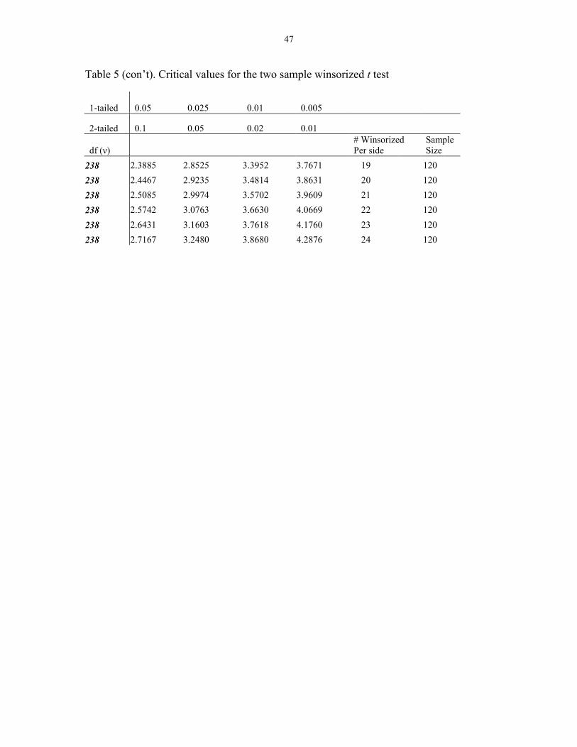
47
Table 5 (con’t). Critical values for the two sample winsorized t test
1-tailed 0.05 0.025 0.01 0.005
2-tailed 0.1 0.05 0.02 0.01
df (ν)
# Winsorized
Per side
Sample
Size
238 2.3885 2.8525 3.3952 3.7671 19 120
238 2.4467 2.9235 3.4814 3.8631 20 120
238 2.5085 2.9974 3.5702 3.9609 21 120
238 2.5742 3.0763 3.6630 4.0669 22 120
238 2.6431 3.1603 3.7618 4.1760 23 120
238 2.7167 3.2480 3.8680 4.2876 24 120

48
CHAPTER 5
DISCUSSION
Overview
Previously, in situations where outliers were present in a data set or the
underlying distribution was in question, asymptotic adjustments had to be made for the
two sample winsorized t test using Student’s t test based on h1 +h2-2 degrees of freedom,
where h is calculated using the formula h = n – 2g, where n represents the sample size
and g represents the number of values winsorized per side. The findings of this study
now make it possible for researchers to reference the distribution of the winsorized t to
get a better estimate of the correct critical value.
To illustrate the efficiency of the critical values derived from approximating the
distribution of the winsorized t, an example was calcualted where two samples were
analyzed using both the Student’s two sample t test and the two sample winsorized t test.
The calculated test statistic was then compared against the critical values from both the
Student’s t distribution Both samples were then comparing the critical values from two
sample t test to those from the two sample winsorized t test using a random data set
where n1 = n2 = 25.

49
Table 6. Random data used for comparison.
SAMPLE A SAMPLE B
-5.84 1.21 -8.75 -0.02
-1.87 1.49 -2.79 0.04
-0.43 1.55 -0.91 0.22
-0.54 1.57 -0.62 0.38
-0.12 1.57 -0.55 0.51
-0.02 1.82 -0.41 0.53
0.12 1.87 -0.40 0.61
0.34 1.90 -0.31 1.09
0.40 1.91 -0.28 1.47
0.53 1.93 -0.21 1.59
0.55 2.34 -0.18 2.39
0.62 3.95 -0.16 2.06
0.92 -0.03
________________________________________________________________________
For each sample, both the two sample t test and winsorized t test were calculated
at the 0.05 level for the two-tailed test to determine if the |T| exceeded the tabled critical
value. If no difference is found to exist between the two treatment groups, the null
hypothesis, Ho: μ1 = μ2 will be retained. The calculated means and standard deviations
for both groups are as follows:
Sample A Sample B
: 0.7108 -0.1892
s: 1.7965 2.0667
Using the formula for the two sample t,
1 2
1 2
2x x
X XtS
n
, where
1 2
1 2
2 2
2
x xx x
S SS
.
The calculated t value, 1.6433, is compared to the critical value of ± 2.0106 from
Student’s t table for df = 48 at α = 0.05 for a two-tailed test. Because the calculated t
value, 1.6433, is less than the critical value, the null hypothesis is maintained, that there
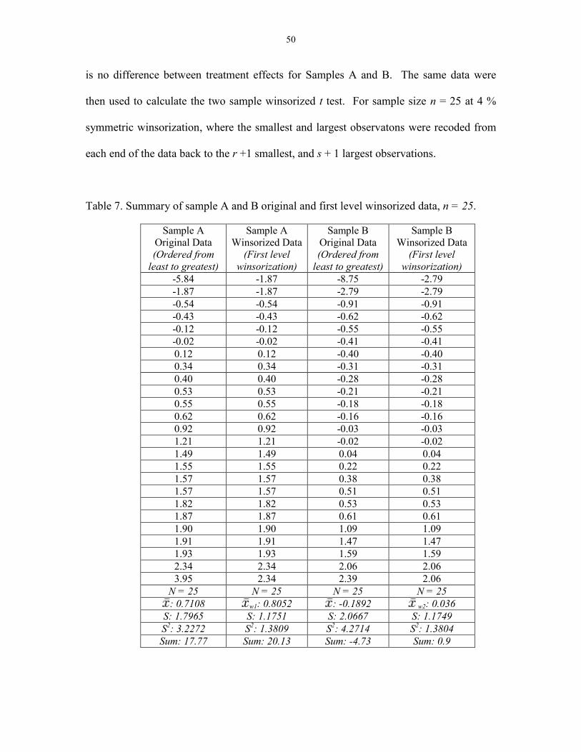
50
is no difference between treatment effects for Samples A and B. The same data were
then used to calculate the two sample winsorized t test. For sample size n = 25 at 4 %
symmetric winsorization, where the smallest and largest observatons were recoded from
each end of the data back to the r +1 smallest, and s + 1 largest observations.
Table 7. Summary of sample A and B original and first level winsorized data, n = 25.
Sample A
Original Data
(Ordered from least to greatest)
Sample A
Winsorized Data
(First level winsorization)
Sample B
Original Data
(Ordered from least to greatest)
Sample B
Winsorized Data
(First level winsorization)
-5.84 -1.87 -8.75 -2.79
-1.87 -1.87 -2.79 -2.79
-0.54 -0.54 -0.91 -0.91
-0.43 -0.43 -0.62 -0.62
-0.12 -0.12 -0.55 -0.55
-0.02 -0.02 -0.41 -0.41
0.12 0.12 -0.40 -0.40
0.34 0.34 -0.31 -0.31
0.40 0.40 -0.28 -0.28
0.53 0.53 -0.21 -0.21
0.55 0.55 -0.18 -0.18
0.62 0.62 -0.16 -0.16
0.92 0.92 -0.03 -0.03
1.21 1.21 -0.02 -0.02
1.49 1.49 0.04 0.04
1.55 1.55 0.22 0.22
1.57 1.57 0.38 0.38
1.57 1.57 0.51 0.51
1.82 1.82 0.53 0.53
1.87 1.87 0.61 0.61
1.90 1.90 1.09 1.09
1.91 1.91 1.47 1.47
1.93 1.93 1.59 1.59
2.34 2.34 2.06 2.06
3.95 2.34 2.39 2.06
N = 25 N = 25 N = 25 N = 25 : 0.7108 w1: 0.8052 : -0.1892 w2: 0.036
S: 1.7965 S: 1.1751 S: 2.0667 S: 1.1749 S2: 3.2272 S2: 1.3809 S2: 4.2714 S2: 1.3804 Sum: 17.77 Sum: 20.13 Sum: -4.73 Sum: 0.9

51
Calculation of the two sample winsorized t is derived using a modification of the
Student’s t test (see p. 31) and is outlined below:
Computation of the numerator: 0.8052 – 0.036 =0 .7692;
Computation of the denominator: =
1 1(25 1)1.3809 (25 1)1.3804
25 25
25 25 2
= (24)1.3809 (24)1.3804) 0.08
48
= (33.1416 33.1296) 0.08
48
= (66.2712) 0.08
48
= (5.301696)
48
= 0.110452 = 0.3323431961 So, tw = 0.7692/0.3323431961 tw = 2.31447 When the calculated winsorized t value, 2.3145, is compared against the critical
value of ± 2.1864 for first level winsorization for 48 df at α = 0.05 for the two-tailed test,
it is observed that the calculated winsorized t value exceeds the critical value. The null

52
hypothesis is then rejected, that there is no difference between treatment effects for
Samples A and B, which is inconsistent with the results achieved from Student’s t test.
Conclusions
The table of critical values developed from this study are useful in that
researchers no longer have to rely on or reference critical values from Student’s t table
when using the two independent samples winsorized t test. As noted in the previous
example, making inferences about data that may be prone to outliers using critical values
from Student’s t table can provide significantly different results than when using critical
values from the winsorized t table. The critcal values for the two independent samples
winsorized t table are useful tools for researchers to reference, particularly in the fields of
psychology and education, where it was noted by Micerri (1989), that many emperical
distributions are prone to extreme heavy tailedness.

53
REFERENCES
Andrews, D.F., Bickel, P.J., Hampel, F.R., Huber, P.J., Rogers, W.H., and Tukey, J.W.
(1972). Robust Estimates of Location: Survey and Advances. Princeton
University Press, Princeton, NJ.
Anscombe, F.J. (1960). Rejection of outliers. Technometrics, 2, 123-147.
Ansell, M. J. G. (1973). Robustness of location estimators to asymmetry. Applied
Statistics, 22, 249-254.
Barnett, V. & Lewis, T. (1984). Outliers in Statistical Data, 2nd ed., Chichester: Wiley.
Bennett, P.J., (2009). Introduction to the Bootstrap and Robust Statistics, 1-11.
Blair, R. C. (1981). A reaction to "Consequences of failure to meet assumptions
underlying the fixed effects analysis of variance and covariance." Review of
Educational Research, 51, 499-507.
Blair, R. C., & Higgins, J. J. (1980a). A comparison of the power of the t test
and the Wilcoxon statistics when samples are drawn from a certain mixed normal
distribution. Evaluation Review, 4, 645-656.
Blair, R. C., & Higgins, J. J. (1980b). A comparison of the power of the
Wilcoxon's rank-sum statistic to that of student's t statistic under various
non-normal distributions. Journal of Educational Statistics, 5, 309-335.
Blair, R. C., & Higgins, J. J. (1981). A note on the asymptotic relative
efficiency of the Wilcoxon rank-sum test relative to the independent means t
test under mixtures of two normal populations. British Journal of Mathematical
and Statistical Psychology, 31, 124-128.
Boneau, C. A. (1960). The effects of violations of assumptions underlying the t

54
test. Psychological Bulletin, 57, 49-64.
Boneau, C. A. (1962). A comparison of the power of the U and t tests. Psychological
Review, 69, 246-256.
Bradley, J. V. (1968). Distribution-free statistical tests. Englewood Cliffs, NJ: Prentice-
Hall.
Bradley, J. V. (1977). A common situation conducive to bizarre distribution shape.
American Statistician, 31, 147-150.
Bradley, J. V. (1978). Robustness? British Journal Mathematical and Statistical
Psychology, 31, 114-152.
Bradley, J. V. (1982). The insidious L-shaped distribution. Bulletin of the Psychometrics
Society, 20(2), 85-88.
Bradley, J. V. (1980). Nonrobustness in Z, t, and F tests at large sample sizes. Bulletin of
the Psychonomic Society, 16, 333–336.
Brown, M. B. and Forsythe, A. B. (1974), Journal of the American Statistical
Association, 69, 364-367.
Carroll, R. J. (1979). On estimating variances of robust estimators when the
errors are asymmetric. Journal of the American Statistical Association, 74, 674-
679.
Chauvenet,W. (1963). Method of least squares. Appendix to Manual of Spherical and
Practical Astronomy, 2, Lippincott, Philadelphia.
Cochran, W. G., & Cox, G. M. (1950). Experimental Design. New York: Wiley.
Cressie, N. Relaxing assumptions in the one sample t-test. Australian Journal of
Statistics, 22, 143-153.
55
David, H. A., & Shu, V. S. (1978). Robustness of location estimators in the presence of
an outlier. In H. A. David (Ed.),Contributions to survey sampling and applied
statistics (pp. 235-250). New York: Academic Press.
Dixon, W.J., (1960). Simplified Estimation from Censored Normal Samples, The Annals
of Mathematical Statistics, 31, 385–391.
Dixon, W.J. & Massey, F. J., (1969). Introduction to statistical analysis. McGraw-Hill,
NewYork.
Dixon, W. J., Tukey, J.W. (1968), Approximate Behavior of the Distribution of
Winsorized t (Trimming/Winsorization 2), Technometrics, (10)1,83-98.
Edgington, E. S. (1995). Randomization Tests. (3d. Ed.) New York: Marcel Dekker.
Efron, B. (1969). Student's t-test under symmetry conditions. Journal of the
American Statistical Association, 64, 1278-1302.
Fisher, R. A. (1935). The Design of Experiments, Edinburgh, U.K.: Oliver & Boyd.
Fortin, M., Jacquez, G., & Shipley, B. (2002). Computer-Intensive Methods.
Encyclopedia of Environmetrics, 1, 399-402.
Fuller, W. A., (1991). Simple estimators for the mean of skewed populations. Statistica
Sinica, 1, 137-158.
Fung, K.Y. & Rahman, S.M. (1980). The Two-Sample Winsorized T. Communications
in Statistics: Simulation and Computation, 89(4), 337-347.
Gastwirth, J. L., & Rubin, H. (1975). The behavior of robust estimators on dependent
data. The Annals of Statistics, 3, 1070-1100.
Gayen, A. K. (1949). The distribution of 'Student' t in random samples of any size drawn
from non-normal universes. Biometrika, 36, 353-369.
56
Gayen, A. K. (1950). The distribution of the variance ratio in random samples of
any size drawn from non-normal universes. Biometrika, 37, 236-255.
Geary, R. C. (1936). The distribution of 'Student's' ratio from non-normal
samples. Journal of the Royal Statistical Society, 3, 178-184.
Geary, R. C. (1947). Testing for normality. Biometrika, 34, 209-242.
Glaisher, J.W.L., (1873). On the rejection of discordant observations. Monthly Notices of
the Royal Astronomical Society., 33, 391-402 (22).
Glass, G. V., Peckham, P. D., & Sanders, J. R. (1972). Consequences of failure to meet
assumptions underlying the analysis of variance and covariance. Review of
Educational Research, 42, 237-288.
Hill, M. A. & Dixon, W. J. (1982). Robustness in real life: A study of clinical laboratory
data. Biometrics, 38, 377-396.
Hoaglin, F. Mosteller F., & Tukey, J. (Eds.) (1982). Understanding Robust and
Exploratory Data Analysis, 404-431. New York: Wiley.
Hogg, R. V. (1974). Adaptive robust procedures: A partial review and some
suggestions for future applications and theory. American Statistical Association
Journal, 69, 909-927.
http://www.engineeredsoftware.com/nasa/images/Image72.gif
Jaeckel, L. A., (1971). Robust Estimates of Location: Symmetry and Asymmetric
Contamination. The Annals of Mathematical Statistics, 42( 3), 1020-1034.
Judd, C. M., & McClelland, G. H. (1989). Data analysis: A model comparison
approach. San Diego, CA.: Harcourt Brace Jovanovich.

57
Kelly, P.A. (1999). Overview of Computer Intensive Statistical Inference Procedures.
Florida State University.
Kerlinger, F. & Lee H., (2000). Foundations of Behavioral Research. Orlando, FL:
Harcourt College Publishers.
Keselman, H.J., Othman, A.R., Wilcox, R.R., & Fradette, K. (2004): The new and
improved two-sample t-test. Psychological Science, 15(1), 57–51.
Kimber, A.C., (1983), Trimming in gamma samples., Journal of the Royal Statistical
Society, Series C, (Applied Statistics), 32, (1), 7-14.
Lindquist, E.F. (1953). Design and analysis of experiments in psychology and education.
Boston, MA: Houghton Mifflin.
Metropolis, N. and Ulam, S. (1949). The Monte Carlo Method. Journal of the American
Statistical Association 44 (247): 335–341.
Micceri, T. (1989). The unicorn, the normal curve, and other improbable creatures.
Psychological Bulletin, 105, 156-166.
Moir, R. (1998). A Monte Carlo Analysis of the Fisher Randomization Technique:
Reviving Randomization for Experimental Economists. Experimental Economics,
1, 87-100.
Noreen, E.W., (1989). Computer Intensive Methods for Testing Hypotheses. New York:
Wiley.
Orr, J. M., Sackett, P. R., & DuBois, C. L. Z. (1991). Outlier detection and treatment in
I/O Psychology: A survey of researcher beliefs and an empirical illustration.
Personnel Psychology, 44, 473-486.

58
Osborne, J.W. & Overbay, A. (2004). The power of outliers (and why researchers should
ALWAYS check for them). Practical Assessment, Research, and Evaluation,
9(6).
Pearson, E. S., & Please, N. W. (1975). Relation between the shape of population
distribution and the robustness of four simple test statistics. Biometrika, 62, 223-
241.
Rivest, L. (1994), Statistical Properties of Winsorized Means for Skewed Distributions.
Biometrika, 81(2), 373-383.
Rosenberger, J. L., & Gasko, M. (1983). Comparing location estimators: Trimmed
means, medians, and trimean. In D. Hoaglin, F. Mosteller & J. Tukey (Eds.)
Understanding Robust and Exploratory Data Analysis, 297-336. New York:
Wiley.
Satterwaite, F. E. (1946). An approximate distribution of estimates of variance
components. Biometrics Bulletin, 2, 110–114.
Sawilowsky, S.S. & Blair, R.C., (1992). A more realistic look at the robustness and Type
II error properties of the t test to departures from population normality.
Psychological Bulletin, 111, 353-360.
Sawilowsky, S.S. & Fahoome, G.C. (2003). Statistics via Monte Carlo Simulation with
Fortran. Rochester Hills, MI: JMASM.
Scheffe, H. (1959). The analysis of variance. New York: Wiley.
Http://www.stats.gla.ac.uk/steps/glossary/hypothesis_testing.html#sl.
Staudte, R.G., & Sheather, S.J. (1990). Robust Estimation and Testing. New York:Wiley.

59
Stigler, S. M. (1977). Do robust estimators work with real data? The Annals of Statistics,
5, 1055-1098.
Tan, W. Y. (1982). Sampling distributions and robustness of t, F and variance-ratio
in two samples and ANOVA models with respect to departure from normality.
Communications in Statistics, A11, 2485-2511.
Tapia, R. A., & Thompson, J. R. (1978). Nonparametric probability density
estimation. Baltimore, MD: Johns Hopkins University Press.
Triola, M. (2006). Elementary Statistics (10th
ed.). Reading, MA: Addison-Wesely
Publishing Company.
Tukey, J. W., & McLaughlin, D. H. (1963). Less vulnerable confidence and significance
procedures for location based on a single sample: Trimming/Winsorization.
Indian Journal of Statistics, 25, 331-351.
Vogt, W. P. (1999). Dictionary of Statistics & Methodology: A Nontechnical Guide for
the Social Sciences. Thousand Oaks, Calif. Sage Publications, Inc.
Wegman, E. J., & Carroll, R. J. (1977). A Monte Carlo study of robust estimators of
location. Communications in Statistics, A6, 795-812.
Welch, B. L. (1947). The generalization of Student’s problem when several different
population variances are involved. Biometrika, 34, 28-35.
Wilcox, R. R. (1990a). Comparing the means of two independent groups. Biometrical
Journal, 32, 771-780.
Wilcox, R. R. (1996). Statistics for the Social Sciences. San Diego: Academic.
Wilcox, R. R. (1996b). A note on testing hypotheses about trimmed means. Biometrical
Journal, 38, 173-180.

60
Wilcox, R.R. & Keselman, H.J. (2003): Modern robust data analysis methods: Measures
of central tendency. American Psychological Association, 8 (3), 254-274.
Wright, T. W. (1884). A Treatise on Adjustments of Observations by the Method of Least
Squares. Van Nostrand, New York.
Yount, W. R. (2006). Research Design and Statistical Analysis in Christian Ministry (4th
Ed.). Fort Worth.
Yuen, K.K., (1974). The two sample trimmed t for unequal population variances.
Biometrika, 61, 165-170.
Yuen, K.K., & Dixon, W. J. (1973). The approximate behavior and performance of the
two-sample trimmed t. Biometrika, 60, 369-374.
Zimmerman, D. (1994). A note on the influence of outliers on parametric and
nonparametric tests. Journal of General Psychology, 121(4), 391.

61
ABSTRACT
CRITICAL VALUES FOR THE TWO INDEPENDENT SAMPLES WINSORIZED T TEST
by
PIPER A. FARRELL-SINGLETON
AUGUST 2010
Advisor: Dr. Shlomo Sawilowsky
Major: (Education, Evaluation and Research)
Degree: Doctor of Philosophy
Through Monte Carlo Simulation, this study explores the approximate behavior of
the two sample winsorized t test. Samples are drawn from the normal population and
symetrically winsorized up to 20%. The two independent samples winsorized t test is
then calculated on each sample using Monte Carlo methods using 1,000,000 iterations.
The t values are then sorted from low to high and the critical values for both one and two
tailed tests identified at the 95th
, 97.5th
, 99th
and 99.5th
percentiles. A table of critical
values is then created, which represents the approximate distribution of the winsorized t
statistic.

62
AUTOBIOGRAPHICAL STATEMENT
PIPER A. FARRELL-SINGLETON
EDUCATION Ed. Spec. Administration and Supervision, Wayne State University • Detroit, MI
B.A. Communication, University of Michigan • Ann Arbor, MI
M.A. Teaching Mathematics, University of Detroit-Mercy • Detroit, MI
PROFESSIONAL EXPERIENCE January 2008 Adjunct Professor, Mathematics • Oakland Community College • Royal Oak/Southfield,
MI.
August 2008
Adjunct Professor, Mathematics • Wayne County Community College • Detroit
Campuses, MI.
August 2007- May 2009
Mathematics Coach • Wayne County RESA/The Morgan Farrell Group, LLC • Detroit,
MI.
October 2003 - September 2007
Mathematics Department Chair • Pershing High School • Detroit, MI
September 1996 - October 2003
Mathematics Teacher • Detroit Public Schools • Detroit, MI
LICENSURE AND CERTIFICATIONS State of Michigan Professional Teaching Certificate • Secondary Level, June, 2004
Mathematics (EX), Speech (BD)
Education Specialist Certificate, Wayne State University, October, 2000
Administration
AWARDS Who’s Who Among American High School Teachers, 2005, 2006.
Distinguished Leadership Award, Pershing High School, June, 2004.
PUBLICATIONS Developing Common Assessments to Target the EXPLORE, PLAN and ACT,
November, 2007.
Detroit Public Schools Algebra 1 and 2 Curriculum Resource Guide, July 2005.