criterion s

7/29/2019 Criterion s

http://slidepdf.com/reader/full/criterion-s 1/3

The all-possible-regressions selection procedure calls for an examination of all possible

regression models involving potential X variables and identifying “good” subsets

according to some criterion.The following can be used:

R2

p criterion

The R 2 p criterion calls for an examination of the coefficient of multiple determination R

2

p in order to select one or several subsets of X variables. We show the number of

parameters in the regression model as a subscript of R 2. Thus, R

2

p indicates that there are

p parameters, or p – 1 predictor variables, in the regression equation on which R2

p is

based.

Since R2

p is a ratio of sums of squares:

(1) R2

p =

SSTO

SSR p= 1 –

SSTO

SSE p

and the denominator is constant for all possible regressions, R2

p varies inversely with the

error sums of squares pSSE . But we know that pSSE can never increase as additional

independent variables are included in the model. Thus, R2

p will be a maximum when all

P – 1 potential X variables are included in the regression model. The reason for using the

R2

p criterion with the all-possible-regressions approach therefore cannot be to maximize

R2

p . Rather, the intent is to find the point where adding more X variables is not

worthwhile because it leads to a very small increase in R2

p . Often, the point is reached

when only a limited number of X variables is included in the regression model. Clearly,the determination of where diminishing returns set in is a judgmental one.

p MSE or R2

a criterion

Since R2

p does not take account of the number of parameter in the model, and since

max( R2

p ) can never decrease as p increases, the use of the adjusted coefficient of multiple

determination R2

a .

(2) R2

a = 1 –

1

11

−−=

−

−

n

SSTO

MSE

SSTO

SSE

pn

n

has been suggested as a criterion which takes the number of parameters in the model into

account through the degrees of freedom. It can be seen from (2) that R2

a increases if and

only if MSE decreases since SSTO/(n – 1) is fixed for the given Y observations. Hence, R2

a and MSE are equivalent criteria. We shall consider here the criterion p MSE . Min(



p MSE ) can, indeed, increase as p increases when the reduction in pSSE becomes so

small that it is not sufficient to offset the loss of an additional degree of freedom. Users of

the p MSE criterion either seek to find the subset of X variables that minimizes p MSE ,

or one or several subsets for which p MSE is so close to the minimum that adding more

variables is not worthwhile.

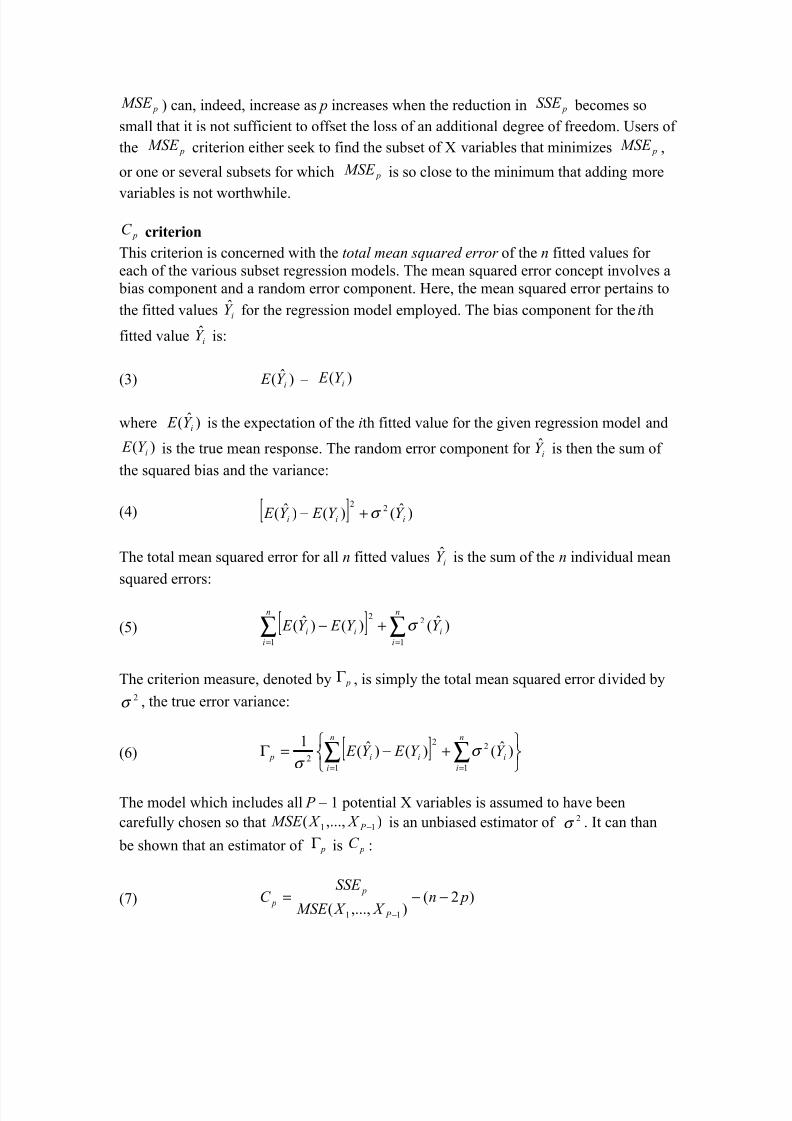
pC criterion

This criterion is concerned with the total mean squared error of the n fitted values for

each of the various subset regression models. The mean squared error concept involves a

bias component and a random error component. Here, the mean squared error pertains to

the fitted values iY ̂ for the regression model employed. The bias component for the ith

fitted value iY ̂ is:

(3) )ˆ( iY E – )( iY E

where )ˆ( iY E is the expectation of the ith fitted value for the given regression model and

)( iY E is the true mean response. The random error component for iY ̂ is then the sum of

the squared bias and the variance:

(4) [ ] )ˆ()()ˆ( 22

iii Y Y E Y E σ +−

The total mean squared error for all n fitted values iY ̂ is the sum of the n individual mean

squared errors:

(5) [ ] ∑∑==

+−n

i

i

n

i

ii Y Y E Y E 1

2

1

2

)ˆ()()ˆ( σ

The criterion measure, denoted by pΓ , is simply the total mean squared error divided by2

σ , the true error variance:

(6) [ ]

+−=Γ ∑ ∑= =

n

i

n

i

iii p Y Y E Y E 1 1

22

2)ˆ()()ˆ(

1σ

σ

The model which includes all P – 1 potential X variables is assumed to have been

carefully chosen so that ),...,( 11 − P X X MSE is an unbiased estimator of 2σ . It can than

be shown that an estimator of pΓ is pC :

(7) )2(),...,( 11

pn X X MSE

SSE C

P

p

p −−=−



where pSSE is the error sum of squares for the fitted subset regression model with p

parameters ( i.e., with p – 1 predictor variables).

When there is no bias in the regression model with p – 1 predictor variables so that

)ˆ( iY E ≡ )( iY E , the expected value of pC is approximately p:

(8) pY E Y E C E ii p ≅≡ )]()ˆ(/[

Thus, when pC values for all possible regression models are plotted against p, those

models with little bias will tend to fall near the line pC = p. Models with substantial bias

will tend to fall considerably above this line.

In using the pC criterion, one seeks to identify subsets of X variables for which (1) the

pC value is small and (2) the pC value is near p. Sets of X variables with small pC

values have a small total mean squared error, and when pC

value is also near p, the biasof the regression model based on the subset of X variables with the smallest pC value

involves substantial bias. In that case, one may at times prefer a regression model based

on somewhat larger subset of X variables for which the pC value is slightly larger but

which does not involve a substantial bias component.About the SAS procedure:

The MAXR methods begins by finding the one-variable model producing the

highest

R (R square). The another variable, the one that would yield the

greatest increase in R is added. Then each of the variables in the

model is compared to each variable not in the model. For each

comparison, MAXR determines if removing one variable and replacing it

with the other variable would increase R.After comparing all possible switches, the one that produces the

largest increase in R is made. And this is continuing in every step.

The all possible regression approach considering all possible models

produces even better results.

criterion s

Documents