crises and recoveries in an empirical model of consumption ...en2198/papers/cdisasters.pdf ·...
TRANSCRIPT

35
American Economic Journal: Macroeconomics 2013, 5(3): 35–74 http://dx.doi.org/10.1257/mac.5.3.35
Crises and Recoveries in an Empirical Model of Consumption Disasters†
By Emi Nakamura, Jón Steinsson, Robert Barro, and José Ursúa*
We estimate an empirical model of consumption disasters using new data on consumption for 24 countries over more than 100 years, and study its implications for asset prices. The model allows for par-tial recoveries after disasters that unfold over multiple years. We find that roughly half of the drop in consumption due to disasters is subsequently reversed. Our model generates a sizable equity pre-mium from disaster risk, but one that is substantially smaller than in simpler models. It implies that a large value of the intertemporal elasticity of substitution is necessary to explain stock-market crashes at the onset of disasters. (JEL E21, E32, E44, G12, G14)
The average return on stocks is roughly 7 percent higher per year than the aver-age return on bills across a large cross-section of countries in the twentieth
century (Barro and Ursúa 2008a). Mehra and Prescott (1985) argued that this large equity premium is difficult to explain in simple consumption-based asset-pricing models. A large subsequent literature in finance and macroeconomics has sought to explain this “equity-premium puzzle.” In recent years, there has been growing inter-est in the notion that the equity premium may be compensation for the risk of rare, but disastrous, events such as wars, depressions, and financial crises (Rietz 1988; Barro 2006).1
In Barro (2006), output is a random walk with drift, and rare disasters are identi-fied as large, instantaneous, and permanent drops in output. He calibrates the fre-quency and permanent impact of disasters to match large peak-to-trough drops in real per capita GDP in a long-term panel dataset for 35 countries, and shows that his model is able to match the observed equity premium with a coefficient of relative risk aversion of the representative consumer of roughly 4. More recently, Barro and
1 Piazzesi (2010) summarizes recent research on the equity premium, emphasizing four main explanations: hab-its (Campbell and Cochrane 1999), heterogeneous agents (Constantinides and Duffie 1996), long-run risk (Bansal and Yaron 2004), and rare disasters.
* Nakamura: Graduate School of Business, Columbia University, 3022 Broadway, New York, NY 10027 (e-mail: [email protected]); Steinsson: Department of Economics, Columbia University, 420 W 118 St., New York, NY 10027 (e-mail: [email protected]); Barro: Department of Economic, Harvard University, Littauer Center, 1805 Cambridge St., Cambridge, MA 02138 (e-mail: [email protected]); Ursúa: Goldman Sachs, 200 West St., New York, NY 10282 (e-mail: [email protected]). We would like to thank Timothy Cogley, George Constantinides, Xavier Gabaix, Ralph Koijen, Martin Lettau, Frank Schorfheide, Efthimios Tsionas, Alwyn Young, Tao Zha, and seminar participants at various institutions for helpful comments and conversations. Barro would like to thank the National Science Foundation for financial support through grant 0849496.
† Go to http://dx.doi.org/10.1257/mac.5.3.35 to visit the article page for additional materials and author disclosure statement(s) or to comment in the online discussion forum.
36 AMErIcAn EcOnOMIc JOurnAL: MAcrOEcOnOMIcs JuLy 2013
Ursúa (2008a) have gathered a long-term dataset for personal consumer expenditure in over 20 countries and shown that the same conclusions hold using these data. A growing literature has adopted this model and calibration of pe rmanent, instanta-neous disasters (e.g., Wachter forthcoming; Gabaix 2008; Farhi and Gabaix 2008; Burnside et al. 2008; Guo 2007; and Gourio 2012).2
An important critique of the Rietz-Barro disasters model calibrated to match the peak-to-trough drops in output or consumption is that it may overstate the riskiness of consumption by failing to incorporate recoveries after disasters (Gourio 2008). A world in which disasters are followed by periods of disproportionately high growth is potentially far less risky than one in which all disasters are permanent. Kilian and Ohanian (2002) emphasize the importance of allowing for large transitory fluctua-tions associated with disasters, such as the Great Depression and WWII, in empirical models of output dynamics. More generally, a large literature in macroeconomics has debated whether it is appropriate to model output as trend or difference- stationary (Cochrane 1988; Cogley 1990).
A second critique of the Rietz-Barro model is that it assumes that the entire drop in output and consumption at the time of a disaster occurs instantaneously. In real-ity, most disasters unfold over multiple years. This profile implies that even though peak-to-trough declines in consumption exceeding 30 percent have occurred in many countries, the annual decline in consumption in these episodes is considerably smaller. Combining persistent declines in consumption into a single event might not be an innocuous assumption. The assumption that the entire decline in output and consumption associated with a disaster occurs in a single year is criticized in Constantinides (2008). Similarly, Julliard and Ghosh (2012) argue that using annual consumption data as opposed to peak-to-trough drops yields starkly different con-clusions from Barro’s original calibration (Barro 2006).3
Given the growing importance of the disasters model in the macroeconomics, international economics, and asset-pricing literatures, a key question is whether it stands up to incorporating a more realistic process for consumption dynamics during and following disasters. We develop a model of consumption disasters that allows disasters to unfold over multiple years and to be systematically followed by recoveries. The model also allows for transitory shocks to growth in normal times and for a correlation in the timing of disasters across countries. This last feature of the model allows us to capture the fact that major disasters, such as the world wars of the twentieth century, affect many countries simultaneously. Ours is the first paper to estimate the dynamic effects—both long term and short term—of these major disasters on consumption.
2 Barro and Jin (2011) show that the required coefficient of relative risk aversion can be reduced to around three if the size distribution of macroeconomic disasters is gauged by an estimated power-law distribution.
3 Julliard and Ghosh (2012) propose a novel approach to estimating the consumption Euler equation based on generalized empirical likelihood methods, in the context of a representative agent consumption-based asset pricing model with time-additive power utility preferences. A key difference between our framework and theirs is that they focus on power utility, as in the original Rietz-Barro framework. We show that allowing for a more general prefer-ence specification is crucial in assessing the asset pricing implications of multi-period disasters and recoveries. Also, our approach does not rely on the exact timing of asset price returns during disasters. As we discuss below, asset price returns during disasters play a disproportionate role in determining the equity premium; yet these are also the periods for which asset price data are most likely to be either missing or inaccurate, for example, because of price controls during wars.
VOL. 5 nO. 3 37Nakamura et al.: Crises aNd reCoveries
We estimate our model on annual consumption data from the newly con-structed Barro and Ursúa (2008a) dataset, using Bayesian Markov-Chain Monte-Carlo (MCMC) methods.4 The model generates endogenous estimates of the timing, magnitude, and length of disasters, as well as the extent of recovery after disasters and the variance of shocks in disaster and nondisaster periods. Our estimation procedure also allows us to investigate the statistical uncertainty associ-ated with the predictions of the rare-disasters model along the lines suggested by Geweke (2007) and Tsionas (2005).5
In estimating the model, we maintain the assumption that the frequency, size dis-tribution, and persistence of disasters is time invariant and the same for all countries. This strong assumption is important in that it allows us to pool information about disasters over time and across countries. The rare nature of disasters makes it dif-ficult to estimate accurately a model of disasters with much variation in structural characteristics over time and space.
We find strong evidence for recoveries after disasters and for the notion that disasters unfold over several years. We estimate that disasters last roughly six years, on average. Over this period, consumption drops, on average, by about 30 percent in the short run. However, about half of this drop in consumption is subsequently reversed. The average long-run effect of disasters on consumption in our data is a drop of about 15 percent.6 We find that uncertainty about future consumption growth increases dramatically at the onset of a disaster. The standard deviation of consump-tion growth in the disaster state is roughly 12 percent per year, several times its value during normal times. The majority of the disasters we identify occur during World War I, the Great Depression, and World War II. Other disasters include the collapse of the Chilean economy, first in the 1970s and again in the early 1980s, and the contraction in South Korea during the Asian financial crisis.
Our estimated model yields asset-pricing results that are intermediate between models that ignore disaster risk and the more parsimonious disaster models con-sidered in the previous literature. We adopt the representative-agent endowment-economy approach to asset pricing—following Lucas (1978) and Mehra and Prescott (1985)—and assume that agents have Epstein-Zin-Weil preferences. Our model matches the observed equity premium with a coefficient of relative risk aversion (CRRA) of 6.4 and an intertemporal elasticity of substitution (IES) of 2. For these parameter values, a model without disasters yields an equity premium only one-tenth as large, while a model with one-period, permanent disasters yields an equity premium ten times larger. Given the close link between the equity pre-mium and the welfare costs of economic fluctuations (Alvarez and Jermann 2004;
4 We use a Metropolized Gibbs sampler. This procedure is a Gibbs sampler with a small number of Metropolis steps. See Gelfand (2000) and Smith and Gelfand (1992) for particularly lucid short descriptions of Bayesian esti-mation methods. See, e.g., Gelman et al. (2004) and Geweke (2005) for comprehensive treatment of these methods.
5 In particular, we analyze the extent to which the observed asset returns are consistent with the posterior dis-tribution of the equity premium implied by our model, taking into account parameter uncertainty. Tsionas (2005) discusses in detail the importance of accounting for finite-sample biases and parameter uncertainty in assessing the ability of alternative models to fit the observed equity premium, particularly in the presence of fat-tailed shocks.
6 Cerra and Saxena (2008) estimate the dynamics of GDP after financial crises, civil wars, and political shocks using data from 1960 to 2001 for 190 countries. They find no recovery after financial crises, and political shocks but partial recovery after civil wars. Their sample does not include World War I, the Great Depression, and World War II. Davis and Weinstein (2002) document a large degree of recovery at the city level after large shocks.

38 AMErIcAn EcOnOMIc JOurnAL: MAcrOEcOnOMIcs JuLy 2013
Barro 2009), these differences imply that our model yields costs of economic fl uctuations s ubstantially larger than a model that ignores disaster risk, but substan-tially smaller than the Rietz-Barro disaster model.
The differences between our model and the more parsimonious Rietz-Barro framework arise both from the recoveries and the multi-period nature of disasters. Recoveries imply that disasters have a much less persistent effect on dividends, reducing the drop in stock prices when disasters occur. This modification, in turn, lowers the equity premium. The multi-period nature of disasters affects the equity premium in a more subtle way. To generate a high-equity premium, the marginal utility of consumption must be high when the price of stocks drops. In our model, the price of stocks crashes at the onset of disasters—with the initial news that a disaster is underway—while consumption typically reaches its trough several years later. This lack of coincidence between the stock market crash and the trough of consumption reduces the equity premium in our model relative to the Rietz-Barro model. In addition, since households anticipate persistent consumption declines at the onset of a disaster—they expect things to get worse before they get better—they have a strong motive to save that does not arise in the Rietz-Barro model. This desire to save limits the magnitude of the stock market decline during disasters, further reducing the equity premium. However, if agents have EZW preferences with crrA > 1 and IEs > 1, the increase in uncertainty about future consumption that occurs at the time of disasters raises marginal utility for a given value of current consumption and, thus, increases the equity premium.
A key feature of our model is the predictability of consumption growth dur-ing disasters—consumption typically declines for several years before recover-ing. These features imply that the IES, which governs consumers’ willingness to trade-off consumption over time, plays an important role in determining the asset-pricing implications of our framework. There is considerable debate in the macroeconomics and finance literature about the value of the IES. Several authors—notably Hall (1988)—argue that the IES is close to zero. However, oth-ers, such as Bansal and Yaron (2004) and Gruber (2006), argue for substantially higher values of the IES.
The large movements in expected consumption growth associated with disasters provide a strong test of consumers’ willingness to substitute consumption over time. For a low value of the IES, our model implies a surge in stock prices at the onset of disasters and a negative equity premium in normal times. The reason is that entering the disaster state generates a strong desire to save, because consumption is expected to fall further in the short run. When the IES is substantially below one, this savings effect dominates the negative effect that the disaster has on expected future divi-dends from stocks and, therefore, raises the price of stocks.7 These predictions do not accord with the available evidence. Disasters are typically associated with stock market crashes. This observation supports the view that consumers have a relatively high willingness to substitute consumption over time (at least during disasters), motivating a high value of the IES.
7 Gourio (2008) makes this point forcefully in a simpler setting. For similar reasons, an IES larger than one plays an important role in the long-run risk model of Bansal and Yaron (2004).
VOL. 5 nO. 3 39Nakamura et al.: Crises aNd reCoveries
Our estimated model yields additional predictions for the behavior of short-term and long-term interest rates. One potential concern is that the same factors driving a high equity premium would also generate a high term premium—a prediction that is not supported by the empirical evidence (Campbell 2003; Barro and Ursúa 2008a). We show that this is not the case. Our model implies a positive equity premium but a negative term premium for risk-free long-term (real) bonds that arises from the hedging properties of long-term bonds during disaster periods. Our model also gen-erates new predictions for the dynamics of risk-free interest rates surrounding disas-ters. In particular, the strong desire to save during disasters drives down the return on short-term bonds, leading to low real interest rates during disaster episodes, as observed in the data.
We consider an extension of our model that allows for partial default on bonds. Empirically, inflation risk is an important source of partial default on govern-ment bonds. Data on stock and bond returns over disaster periods indicate that short-term bonds provide substantial insurance against disaster risk in only about 70 percent of cases. When we allow for an empirically realistic degree of default on short-term bonds, a risk aversion parameter of 7.5 is needed to fit the observed equity premium. Because inflation unfolds sluggishly in the data, the effect of inflation risk on short-term bonds is less severe than on long-term bonds. Incorporating this fact allows us to match the upward-sloping term premium for nominal bonds.
We employ the Mehra and Prescott (1985) methodology for assessing the asset-pricing implications of our model. Hansen and Singleton (1982) pioneered an alternative methodology based on measuring the empirical correlation between asset returns and the stochastic discount factor. An important difficulty with employing the Hansen-Singleton approach is that the observed timing of real returns on stocks and bonds relative to drops in consumption during disasters is affected by gaps in the data on asset prices, as well as price controls, asset price controls, and market closure. For example, stock price data are missing for Mexico in 1915–1918, Austria in World War II, Belgium in World War I and World War II, Portugal in 1974–1977, and Spain in 1936–1940. The Nazi regime in Germany imposed price controls in 1936 and asset-price controls in 1943 that lapsed only in 1948. In France, the stock market closed in 1940–1941 and price controls affected measured real returns over a longer period. Given these data limitations, Barro and Ursúa (2009a) take the approach of computing the covariance between the peak-to-trough decline in asset prices and a consumption-based stochastic discount fac-tor using a “flexible timing” assumption regarding the intervals over which these declines occur. Under this assumption, it is possible to match the equity premium for moderate values of risk aversion. Their calculations highlight the dispropor-tionate importance of disasters in matching the equity premium. Nondisaster periods contribute trivially to the equity premium.8
8 Another concern regarding the Hansen-Singleton methodology, emphasized by Geweke (2007) and Arakelian and Tsionas (2009), is that parsimonious asset pricing models are sufficiently stylized so that formal statistical rejections may not be very informative.
40 AMErIcAn EcOnOMIc JOurnAL: MAcrOEcOnOMIcs JuLy 2013
A number of recent papers study whether the presence of rare disasters may also help to explain other anomalous features of asset returns, such as the predictabil-ity and volatility of stock returns. These papers include Farhi and Gabaix (2008), Gabaix (2008), Gourio (2008), and Wachter (forthcoming). Martin (2008) presents a tractable framework for asset pricing in models of rare disasters. Gourio (2012) embeds disaster risk in a business-cycle model and shows that time-varying disaster risk can generate joint dynamics of macroeconomic aggregates and asset prices that are consistent with the data.
The paper proceeds as follows. Section I discusses the Barro-Ursúa data on long-term personal consumer expenditures. Section II presents the empirical model. Section III discusses our estimation strategy. Section IV presents our empirical esti-mates. Section V studies the asset-pricing implications of our model. Section VI concludes.
I. Data
In estimating our disaster model, it is crucial to use long time series whose start-ing and ending points are not endogenous to the disasters themselves. It is also crucial that the dataset contain information on the evolution of macroeconomic vari-ables during disasters; Maddison’s (2003) tendency to interpolate GDP data during wars and other crises is not satisfactory for our purposes. Furthermore, to analyze the asset-pricing implications of rare disasters, it is important to measure consump-tion dynamics, as opposed to output dynamics.
We use a recently created dataset on long-term personal consumer expenditures constructed by Barro and Ursúa and described in detail in Barro and Ursúa (2008a).9 This dataset includes a country only if uninterrupted annual data are available back at least before World War I, yielding a sample of 17 Organisation for Economic Co-operation and Development (OECD) countries and 7 non-OECD countries.10 To avoid sample selection bias problems associated with the starting dates of the series, we include only data after 1890. The resulting dataset is an unbalanced panel of annual data for 24 countries, with data from each country starting between 1890 and 1914 and ending in 2006, yielding a total of 2,685 observations.
One limitation of the Barro-Ursúa consumption dataset is that it does not allow us to distinguish between expenditures on nondurables and services versus durables. Unfortunately, separate data on durable and nondurable consumption are not avail-able for most of the countries and time periods we study. For time periods when such data are available, however, the effect of excluding durables on the overall decline in consumer spending during disasters is small. The proportionate decline in spending on nondurables and services is, on average, only 3 percentage points
9 These data are available from Barro’s website, at: http://www.economics.harvard.edu/faculty/barro/data_ sets_barro.
10 The OECD countries are: Australia, Belgium, Canada, Denmark, Finland, France, Germany, Italy, Japan, Netherlands, Norway, Portugal, Spain, Sweden, Switzerland, the United Kingdom, and the United States. The “non-OECD” countries are Argentina, Brazil, Chile, Mexico, Peru, South Korea, and Taiwan. See Barro and Ursúa (2008a) for a detailed description of the available data and the countries dropped due to missing data. In cases where there is a change in borders, as in the case of the unification of East and West Germany, Barro, and Ursúa (2008a) smoothly paste together the initial per capita series for one country with that for the unified country.

VOL. 5 nO. 3 41Nakamura et al.: Crises aNd reCoveries
smaller than the overall decline in consumer spending (Barro and Ursúa 2008a). The reason is that for most of the time period we study, durables accounted for only a small fraction of consumer expenditures. The effect of excluding durables is even smaller during the largest disasters, because durable consumer expenditures can at most fall to zero. The remaining fall in consumer expenditures must come entirely from nondurable expenditures.
In analyzing the asset-pricing implications of our model, we make use of total returns data on stocks, bills, and bonds from Global Financial Data (GFD), aug-mented with data from Dimson, Marsh, and Staunton (2002) and other sources. These data are described in detail in Barro and Ursúa (2009a). Unfortunately, these data are less comprehensive than the corresponding consumption series and often contain gaps for disaster periods. Price controls and controls on asset prices also make the exact timing of real returns difficult to measure during disasters. We therefore use these data to assess the predictions of our model primarily by considering average returns in nondisaster periods and cumulative returns over disaster periods.
II. An Empirical Model of Consumption Disasters
We model log consumption as the sum of three unobserved components:
(1) c i, t = x i, t + z i, t + ϵ i, t ,
where c i, t denotes log consumption in country i at time t, x i, t denotes “potential” consumption in country i at time t; z i, t denotes the “disaster gap” of country i at time t—i.e., the amount by which consumption differs from potential due to current and past disasters; and ϵ i, t denotes an independently and identically disributed normal shock to log consumption with a country-specific variance σ ϵ, i, t 2
that potentially var-ies with time.
The occurrence of disasters in each country is governed by a Markov process I i, t . Let I i, t = 0 denote “normal times” and I i, t = 1 denote times of disaster. The probabil-ity that a country that is not in the midst of a disaster will enter the disaster state is made up of two components: a world component and an idiosyncratic component. Let I W, t be an independently and identically distributed indicator variable that takes the value I W, t = 1 with probability p W . We will refer to periods in which I W, t = 1 as periods in which “world disasters” begin. The probability that a country not in a disaster in period t − 1 will enter the disaster state in period t is given by p cbW I W, t + p cbI (1 − I W, t ), where p cbW is the probability that a particular country will enter a disaster when a world disaster begins, and p cbI is the probability that a particular country will enter a disaster “on its own.” Allowing for correlation in the timing of disasters through I W, t is important for accurately assessing the statistical uncertainty associated with the probability of entering the disaster state. Once a country is in a disaster, the probability that it will exit the disaster state each period is p ce .
We model disasters as affecting consumption in two ways. First, disasters cause a large short-run drop in consumption. Second, disasters may affect the level of

42 AMErIcAn EcOnOMIc JOurnAL: MAcrOEcOnOMIcs JuLy 2013
potential consumption to which the level of actual consumption will return. We model these two effects separately. First, let θ i, t denote a one-off permanent shift in the level of potential consumption due to a disaster in country i at time t. Second, let ϕ i, t denote a shock that causes a temporary drop in consumption due to the disas-ter in country i at time t. For simplicity, we assume that θ i, t does not affect actual consumption on impact, while ϕ i, t does not affect consumption in the long run. In this case, θ i, t may represent a permanent loss of time spent on R&D and other activities that increase potential consumption or a change in institutions that the disaster induces. The short-run shock, ϕ i, t , could represent destruction of structures, crowding out of consumption by government spending, and temporary weakness of the financial system during the disaster.
We assume that θ i, t is distributed θ i, t ∼ N(θ, σ θ 2 ). This implies that we do not rule out the possibility that disasters can have positive long-run effects. Crises can, e.g., lead to structural change that benefits the country in the long run. We consider two distributional assumptions for the short-run shock ϕ i, t . Both of these distributions are one-sided, reflecting our interest in modeling disasters. In our baseline case, ϕ i, t has a truncated normal distribution on the interval [−∞, 0]. We denote this as ϕ i, t ∼ tN( ϕ ∗ , σ ϕ ∗2 , −∞, 0), where ϕ ∗ and σ ϕ ∗2 denote the mean and variance, respectively, of the underlying normal distribution (before truncation). We use ϕ and σ ϕ 2
to denote the mean and variance of the truncated distribution. We also estimate a model with − ϕ i, t ∼ Gamma( α ϕ , β ϕ ). The gamma distribution is a flexible one-sided distribution that has excess kurtosis relative to the normal distribution.
Potential consumption evolves according to
(2) Δ x i, t = μ i, t + η i, t + I i, t θ i, t ,
where Δ denotes a first difference, μ i, t is a country-specific average growth rate of trend consumption that may vary over time, η i, t is an independently and identically distributed normal shock to the growth rate of trend consumption with a country specific variance σ η, i 2
. This process for potential consumption is similar to the pro-cess assumed by Barro (2006) for actual consumption. Notice that consumption in our model is trend stationary if the variances of η i, t and θ i, t are zero.
The disaster gap follows an AR(1) process:
(3) z i, t = ρ z z i t−1 − I i, t θ i, t + I i, t ϕ i, t + ν i, t ,
where 0 ≤ ρ z < 1 denotes the first order autoregressive coefficient and ν i t is an independently and identically distributed normal shock with a country-specific variance σ ν i 2
. We introduce ν i t mainly to aid the convergence of our numerical algorithm.11 Since θ i, t is assumed to affect potential consumption, but to leave actual
11 MCMC algorithms have trouble converging when the objects one is estimating are highly correlated. In our case, z t and z t+j for small j are highly correlated when there are no disturbances in the disaster gap equation between time t and time t + j. This would be the case in the “no disaster” periods in our model if it did not include the ν i, t
VOL. 5 nO. 3 43Nakamura et al.: Crises aNd reCoveries
consumption unaffected on impact, it gets subtracted from the disaster gap when the disaster occurs.
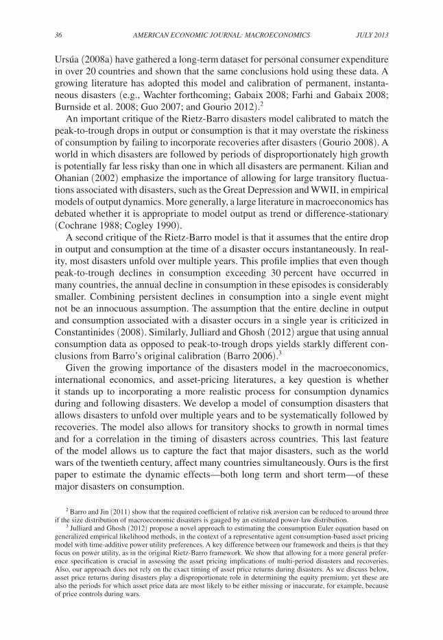
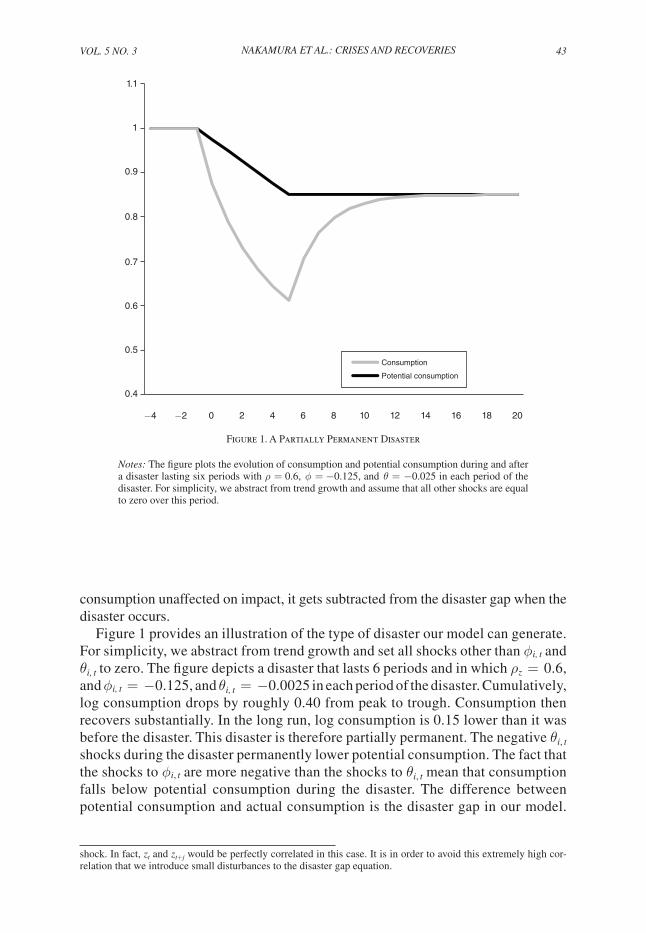
Figure 1 provides an illustration of the type of disaster our model can generate. For simplicity, we abstract from trend growth and set all shocks other than ϕ i, t and θ i, t to zero. The figure depicts a disaster that lasts 6 periods and in which ρ z = 0.6, and ϕ i, t = −0.125, and θ i, t = −0.0025 in each period of the disaster. Cumulatively, log consumption drops by roughly 0.40 from peak to trough. Consumption then recovers substantially. In the long run, log consumption is 0.15 lower than it was before the disaster. This disaster is therefore partially permanent. The negative θ i, t shocks during the disaster permanently lower potential consumption. The fact that the shocks to ϕ i, t are more negative than the shocks to θ i, t mean that co nsumption falls below potential consumption during the disaster. The difference between potential consumption and actual consumption is the disaster gap in our model.
shock. In fact, z t and z t+j would be perfectly correlated in this case. It is in order to avoid this extremely high cor-relation that we introduce small disturbances to the disaster gap equation.
Consumption
Potential consumption
−4 −2 0 2 4 6 8 10 12 14 16 18 20
1.1
1
0.9
0.8
0.7
0.6
0.5
0.4
Figure 1. A Partially Permanent Disaster
notes: The figure plots the evolution of consumption and potential consumption during and after a disaster lasting six periods with ρ = 0.6, ϕ = −0.125, and θ = −0.025 in each period of the disaster. For simplicity, we abstract from trend growth and assume that all other shocks are equal to zero over this period.

44 AMErIcAn EcOnOMIc JOurnAL: MAcrOEcOnOMIcs JuLy 2013
In the long run, the disaster gap closes—i.e., consumption recovers—so that only the drop in potential consumption has a long-run effect on consumption. Our model can generate a wide range of paths for consumption during a disaster. If θ i, t = 0 throughout the disaster, the entire disaster is transitory. If, on the other hand, ϕ i, t = θ i, t throughout the disaster, the entire disaster is permanent.
A striking feature of the consumption data is the dramatic drop in volatility in many countries following Word War II. Part of this drop in consumption volatility likely reflects changes in the procedures for constructing national accounts that were implemented at this time (Romer 1986; Balke and Gordon 1989). We allow for this break by assuming that σ ϵ, i, t 2
takes two values for each country: one before 1946 and one after. Allowing for this feature is important in not overestimating the occurrence of disasters in the early part of the sample. Another striking feature is that many countries experienced very rapid growth for roughly 25 years after World War II. We allow for this by assuming that μ i, t takes three values for each country: one before 1946, one for the period 1946–1972, and one for the period since 1973.12 We discuss the implications of allowing for such trend breaks in Section IV.
One can show that the model is formally identified except for a few special cases in which multiple shocks have zero variance. Nevertheless, the main chal-lenge in estimating the model is the relatively small number of disaster episodes observed in the data. We, therefore, assume that all the disaster parameters— p W , p cbW , p cbI , p ce , ρ z , θ , σ θ 2 , ϕ , σ ϕ 2
—are common across countries and time periods. This assumption allows us to pool information about the disasters that have occurred in different countries and at different times. In contrast, we allow the nondisaster parameters— μ i , t , σ ϵ, i, t 2
, σ η, i, t 2 , σ ν , i 2
—to vary across countries.
III. Estimation
The model presented in Section II decomposes consumption into three unob-served components: potential consumption, the disaster gap, and a transitory shock. One way of viewing the model is, thus, as a disaster filter. Just as business-cycle filters isolate movements in output attributable to the business cycle, our model iso-lates movements in consumption attributable to disasters. Despite the large number of unobserved states and parameters, it is possible to estimate our model efficiently using Bayesian MCMC methods.13
12 See Perron (1989) and Kilian and Ohanian (2002) for a discussion of trend breaks in macroeconomic aggregates.
13 Bayesian MCMC methods have recently been applied to many problems in finance in which it is necessary to estimate a large number of unobserved states (see, e.g., Pesaran, Pettenuzzo, and Timmermann 2006; Koop and Potter 2007). An important technical reason that Bayesian MCMC methods work well in our setting is that many of the unobserved states can be sampled using a Gibbs sampler as opposed to more computationally costly meth-ods. Our algorithm samples from the posterior distributions of the parameters and states using a Gibbs sampler augmented with Metropolis steps when needed. This algorithm is described in greater detail in online Appendix A. The estimates discussed in Section IV for both versions of the model, are based on four independent Markov chains each with two million draws with the first 150,000 draws from each chain dropped as burn-in. The four chains are started from two different starting values, two chains from each starting value. We choose these two sets of start-ing values to be far apart in a sense made precise in the online Appendix. We use a number of techniques to assess convergence. First, we employ Gelman and Rubin’s (1992) approach to monitoring convergence based on parallel chains with “ over-dispersed starting points” (see also Gelman et al. 2004, chapter 11). Second, we calculate the
VOL. 5 nO. 3 45Nakamura et al.: Crises aNd reCoveries
To carry out our Bayesian estimation we need to specify a set of priors on the parameters of the model. The full set of priors we use is
θ ∼ N(0, 0.2), σ θ ∼ U(0.01, 0.25), ϕ ∗ ∼ U(−0.25, 0), σ ϕ ∗ ∼ U(0.01, 0.25),ϕ ∼ U(−0.25, 0), σ ϕ ∼ U(0.01, 0.25), p W ∼ U(0, 0.1), p cbI ∼ U(0, 0.02), p cbW ∼ U(0, 1), 1 − p ce ∼ U(0, 0.9), ρ z ∼ U(0, 0.9), μ i, t ∼ N(0.02, 1), σ ϵ i t ∼ U(0, 0.15), σ η i ∼ U(0, 0.15), σ ν i ∼ U(0, 0.015).
We consider two specifications for the short-run shock ϕ i, t : a truncated normal dis-tribution and a gamma distribution. Thus, we specify two sets of priors for this shock. For the case of ϕ i, t shocks that have a truncated normal distribution, we specify priors on ϕ ∗ and σ ϕ ∗ —the mean and standard deviation of the normal distribution before it is truncated. For the alternative case with gamma distributed ϕ i, t shocks, we place priors on the mean and standard deviation of ϕ i, t , which we denote as ϕ and σ ϕ . These priors imply a joint prior distribution over α ϕ and β ϕ .
A key parameter in our model is θ, the mean long-run effect of the disaster shock, which determines the extent of recovery from a disaster. Our prior for this param-eter is symmetric and highly dispersed. Thus, the prior is agnostic about whether disasters have any long-run effect at all, and allows for the possibility that in some cases the long-run effect of a disaster might actually be positive, as could arise if the disaster led to a favorable change in institutions. Our estimated long-run effect of disasters thus comes entirely from the data.
Our priors on the probability of disasters embed the assumption that disasters are in fact rare. On the one hand, we do not wish to “overestimate” the probability of disasters by choosing a prior on disasters that places a large prior weight on high disaster frequencies. On the other hand, we do not wish to choose a prior that constrains the posterior distribution of disasters from above. In fact, our results are relatively insensitive to allowing for more dispersed priors on the probability of disasters, since the probability of disasters is essentially pinned down by the fre-quency of large and unusual events (wars, depressions, and financial crises).
Importantly, our priors in no way downweight the possibility that there are no rare disasters in the data generating process, or that the disasters are in fact small. Thus, our results on the importance of disasters are in no sense “built in” to our priors. We further verify this in Section V by re-estimating the model using artificial data generated from a model without disasters. We show that if the model were truly generated by a process without disasters, our model would deliver a tight posterior around zero on the importance of disasters for asset prices—in stark contrast to our results based on estimating the model using actual data.
“effective” sample size (corrected for autocorrelation) for the parameters of the model. Finally, we visually evaluate “trace” plots from our simulated Markov chains.

46 AMErIcAn EcOnOMIc JOurnAL: MAcrOEcOnOMIcs JuLy 2013
We limit the scope of disasters by setting an upper bound on the half-life of the disaster gap. This restriction rules out the possibility that consumption growth in a given period can be explained by disasters that occurred decades earlier.14 We also place upper bounds on the frequency of disasters. Our results are not sensitive to this assumption. Finally, recall that ν i, t is introduced mainly to aid numerical conver-gence of our MCMC sampling algorithm. We therefore restrict its magnitude such that it has a negligible effect on the predictions of the model.
We have extensively investigated the robustness of our asset pricing results to alternative specifications of the priors. For example, priors that restrict disasters to occur less frequently yield similar results because these specifications still allow for the infrequent occurrence of very large disasters, which contribute most to the equity premium.
IV. Empirical Results
Table 1 presents our estimates of the disaster parameters for our baseline case. For each parameter, we present the parametric form of the prior distribution, the mean of the prior and its standard deviation, as well as the posterior mean and pos-terior standard deviation. We refer to the posterior mean of each parameter as our point estimate for that parameter.
The principle new features of our model relative to the Rietz-Barro model of permanent, instantaneous disasters are the possibility of recoveries after disasters, and the notion that disasters may unfold over several years. We find strong empiri-cal support for both of these features. We can gauge the extent to which our results imply that disasters are followed by recoveries by comparing our estimate of ϕ , the mean of the short-run shock ϕ i, t , and θ, the mean of the long-run shock θ i, t . We esti-mate ϕ = −0.111, while we estimate θ = −0.025. This implies that the short-term negative shock to consumption during disasters is, on average, 11.1 percent per year, while the long-run negative impact of the disaster on consumption is only 2.5 percent per year. In other words, most disasters are followed by substantial recoveries.
14 This approach is analogous to one used in the asset-pricing literature of placing restrictions on jumps in returns and volatility (Eraker, Johannes, and Polson 2003).
Table 1—Disaster Parameters
Prior dist. Prior mean Prior SD Post. mean Post SD
p W Uniform 0.050 0.029 0.037 0.016 p cbW Uniform 0.500 0.289 0.623 0.076 p cbI Uniform 0.050 0.029 0.006 0.0031− p ce Uniform 0.500 0.289 0.835 0.027 ρ z Uniform 0.450 0.260 0.500 0.034ϕ Uniform* −0.176 0.064 −0.111 0.008θ Normal 0.000 0.200 −0.025 0.007 σ ϕ Uniform* 0.098 0.047 0.083 0.006 σ θ Uniform 0.130 0.069 0.121 0.015
notes: We specify uniform priors on ϕ ⁎ and σ ϕ ⁎ , the mean and standard deviation of the under-lying normal distribution (before truncation). These priors imply (nonuniform) priors on ϕ and σ ϕ . The numbers in the table refer to the prior mean and standard deviation of ϕ and σ ϕ .

VOL. 5 nO. 3 47Nakamura et al.: Crises aNd reCoveries
Our estimate of p ce —the probability that a country exits a disaster once one has begun—provides strong support for the notion that disasters unfold over s everal years. According to our estimates, a country that is already in a disaster will con-tinue to be in the disaster in the following year with a 0.835 probability. This esti-mate implies that the average length of disasters is roughly six years, while the median length of disasters is four years.
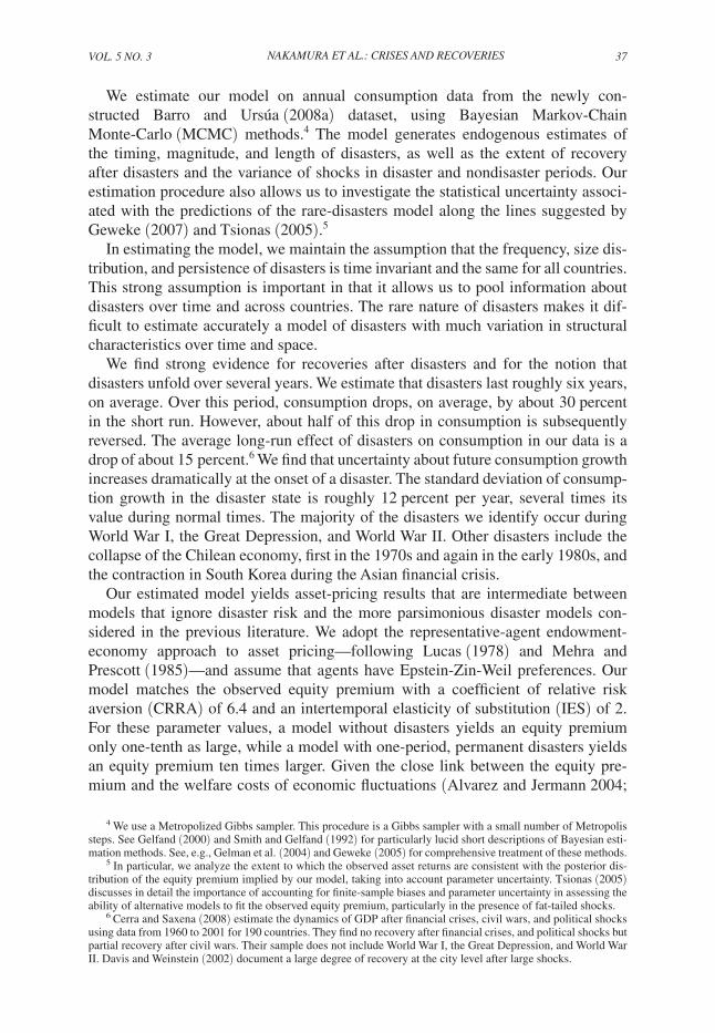
To get a better sense for what these parameters imply about the nature of con-sumption disasters, Figure 2 plots the impulse response of a “typical disaster.” This prototype lasts for six years, and the sizes of the short-run and long-run effects are set equal to the respective posterior means of these parameters for each of the six disaster years (i.e., ϕ i, t = ϕ and θ i, t = θ). The figure shows that the maximum short-run effect of this typical disaster is approximately a 27 percent fall in consumption (a 0.32 fall in log consumption), while the long-run negative effect of the disaster is approximately 14 percent.15
15 The maximum drop is “only” roughly twice the size of the long-run drop even though the average size of the short-run shocks is more than four times larger than the average size of the long-run shock. This is because the effect of the short-run shocks in the first few years of the disaster have largely died out by the end of the disaster.
−0.35
−0.3
−0.25
−0.2
−0.15
−0.1
−0.05
0
Response of log C
Years
1 2 3 4 5 6 7 8 9 10 11 12 13 14 15 16 17 18 19 200
Figure 2. A Typical Disaster
notes: The figure plots the evolution of log consumption during and after a disaster that strikes in period 1 and lasts for six years. Over the course of the disaster, both ϕ and θ take values equal to their posterior means in each period. For simplicity, we abstract from trend growth and assume that all other shocks are equal to zero over this period.
48 AMErIcAn EcOnOMIc JOurnAL: MAcrOEcOnOMIcs JuLy 2013
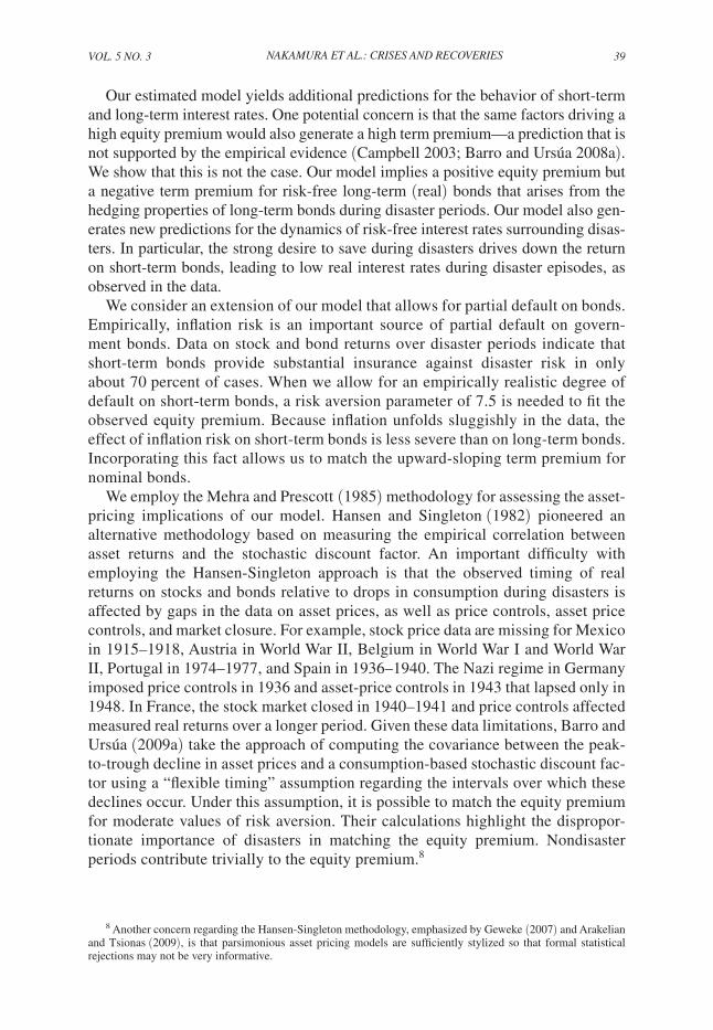
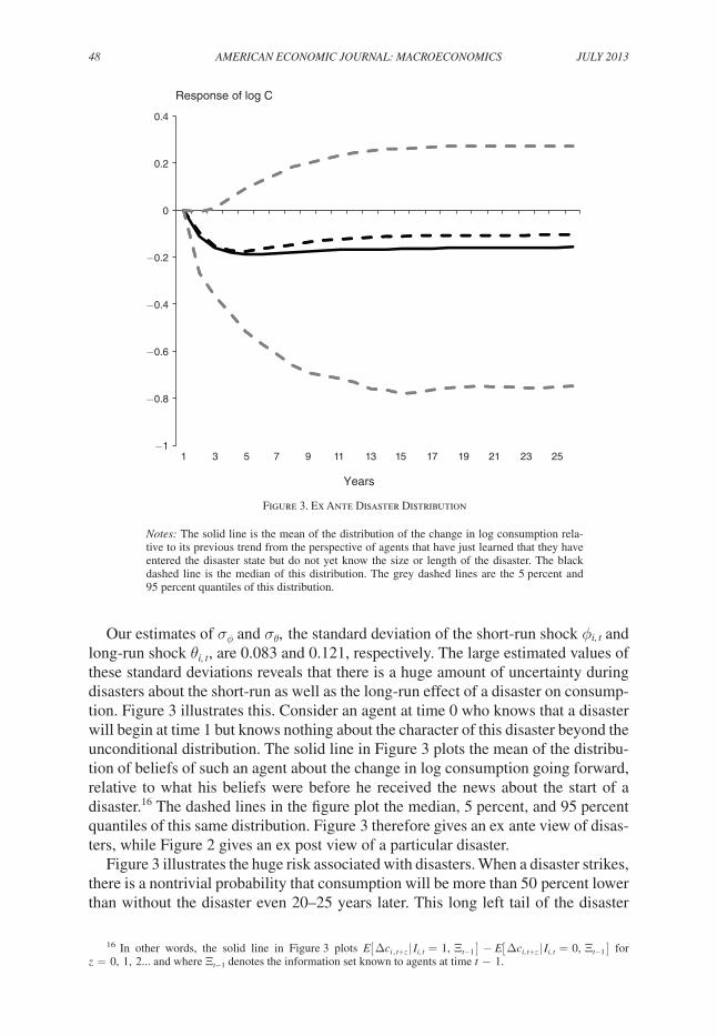
Our estimates of σ ϕ and σ θ , the standard deviation of the short-run shock ϕ i, t and long-run shock θ i, t , are 0.083 and 0.121, respectively. The large estimated values of these standard deviations reveals that there is a huge amount of uncertainty during disasters about the short-run as well as the long-run effect of a disaster on consump-tion. Figure 3 illustrates this. Consider an agent at time 0 who knows that a disaster will begin at time 1 but knows nothing about the character of this disaster beyond the unconditional distribution. The solid line in Figure 3 plots the mean of the distribu-tion of beliefs of such an agent about the change in log consumption going forward, relative to what his beliefs were before he received the news about the start of a disaster.16 The dashed lines in the figure plot the median, 5 percent, and 95 percent quantiles of this same distribution. Figure 3 therefore gives an ex ante view of disas-ters, while Figure 2 gives an ex post view of a particular disaster.
Figure 3 illustrates the huge risk associated with disasters. When a disaster strikes, there is a nontrivial probability that consumption will be more than 50 percent lower than without the disaster even 20–25 years later. This long left tail of the disaster
16 In other words, the solid line in Figure 3 plots E [ Δ c i , t+z | I i, t = 1, Ξ t−1 ] − E [ Δ c i, t+z | I i, t = 0, Ξ t−1 ] for z = 0, 1, 2... and where Ξ t−1 denotes the information set known to agents at time t − 1.
−1
−0.8
−0.6
−0.4
−0.2
0
0.2
0.4
Response of log C
Years
3 5 7 9 11 13 15 17 19 21 23 251
Figure 3. Ex Ante Disaster Distribution
notes: The solid line is the mean of the distribution of the change in log consumption rela-tive to its previous trend from the perspective of agents that have just learned that they have entered the disaster state but do not yet know the size or length of the disaster. The black dashed line is the median of this distribution. The grey dashed lines are the 5 percent and 95 percent quantiles of this distribution.

Vol. 5 No. 3 49Nakamura et al.: Crises aNd reCoveries
distribution is particularly important for asset pricing. The median long-run effect is smaller than the mean long-run effect because the distribution of disaster sizes is negatively skewed. At first glance, Figure 3 seems to suggest more permanence in disasters than the typical disaster graph in Figure 2. This pattern arises because the average short-run effect depicted in Figure 3 averages over many disasters of vary-ing lengths and is, therefore, muted relative to the individual disasters, which reach their troughs at different points in time.17
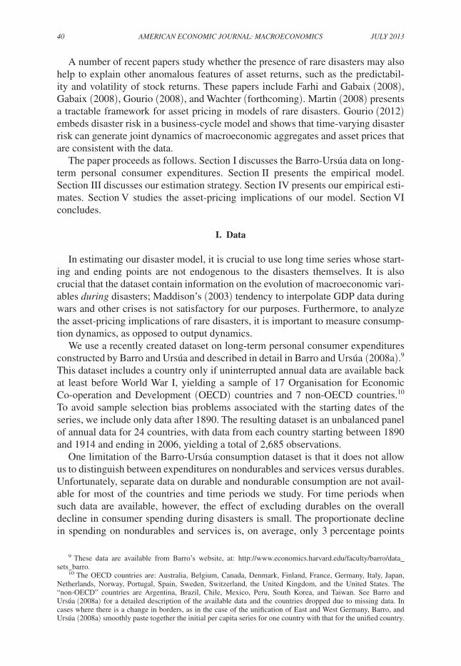
Figure 4 provides more detail about how our model interprets the evolution of consumption for France, Korea, Chile, and the United States.18 The two lines in each panel plot consumption and our estimate of potential consumption. The bars give our posterior probability estimate that a country was in a disaster in each year. For France, the model picks up World War I and World War II as disasters. The model views World War II as largely a transitory event for French consumption. The per-manent effect of World War II on French consumption is estimated to be only about 7 percent. The French experience in World War II is typical for many European countries. For South Korea, our model interprets the entire period from 1940 to 1960
17 For example, a short disaster may reach its trough after two years, while a long disaster may reach its trough after ten years. The average drop in consumption at a given point in time (relative to the start of the disaster) is an average over some disaster paths for which consumption is already recovering after having reached its trough at an earlier point, and other disaster paths for which consumption is still falling toward a later trough. The trough in aver-age consumption is, therefore, far less severe than the average of the troughs across different disasters. In contrast, the long-run average level of consumption is equal to the average of the long-run levels of consumption across the different disaster paths. It is the fact that the trough in average consumption is so much less than the average of the troughs that makes the average disaster path look more permanent than in the case of the prototype disaster.
18 More detailed figures for all the countries in our study are reported in online Appendix C.
0.0
0.4
0.8
2.0
3.0
4.0
0.0
0.4
0.8
2.5
3.5
4.5
1920 1940 1960 1980 2000Year
1920 1940 1960 1980 20001900Year
1920 1940 1960 1980 20001900Year
1920 1940 1960 1980 20001900Year
0.0
0.4
0.8
0.0
0.4
0.8
2.5
3.5
4.5
3.0
3.5
4.0
4.5
United States
Chile
Korea
France
Figure 4. Consumption, Potential Consumption, and Disasters in France, Korea, Chile, and the United States
Note: In each panel, the dark line is log per capita potential consumption, the lighter line is log per capital poten-tial consumption, and the bars give our posterior probability estimate that the country was in a disaster in each year.
50 AMErIcAn EcOnOMIc JOurnAL: MAcrOEcOnOMIcs JuLy 2013
as a single long disaster that spans World War II and the Korean War. In contrast to the experience of many European countries, our estimates suggest that the crisis in the 1940s and 1950s had a large, permanent effect on South Korean consump-tion (48 percent). This pattern is typical of the experience of Asian countries in our sample during World War II.
While the bulk of the disasters we identify are associated with world disasters, we also identify a number of idiosyncratic disaster events. Some of these idiosyncratic disasters are associated with financial or debt crises. For example, we identify a disaster in South Korea at the time of the Asian Financial Crisis and in Argentina at the time of their 2002 sovereign default.19 Other idiosyncratic disasters are associ-ated with regional wars, coups, or revolutions. These include Chile’s experience during the 1970s.
The last panel in Figure 4 plots results for the United States. Relative to most other countries in our sample, the United States was a tranquil place during our sample period. The model identifies two disaster episodes for the United States. The first disaster begins in 1914 and lasts until 1922, encompassing both World War I and the Great Influenza Epidemic of 1918–1920. The Great Depression is identi-fied as a second disaster for US consumption. The Great Depression is the larger of the two disasters with a 26 percent short-run drop in consumption and a 14 percent long-run drop.
One could also ask whether the relative tranquility of the US experience since the Great Depression provides evidence that the United States is fundamentally dif-ferent from other countries in our sample. However, the posterior probability for a randomly selected country experiencing no disasters over a 72-year stretch is 0.12 according to our model. The posterior probability of at least one out of 24 countries experiencing no disaster over a 73-year stretch is 0.60. Therefore, the tranquility of the US experience (which is not randomly selected) does not provide evidence against our model.
Figure 5 plots our estimates of the probability that a “world disaster” began in each year.20 Our model clearly identifies World War I, the Great Depression, and World War II as world disasters. Our estimate of p W , the probability that a world disaster begins, is 3.7 percent per year. Countries are estimated to have a 62.3 p ercent probability of entering disasters conditional on a world disaster, but a much lower (0.6 percent per year) probability of entering a disaster “on their own.” The overall probability that a country enters a disaster is 2.8 percent per year.21
Our Bayesian estimation procedure does not deliver a definitive judgment on whether a disaster occurred at certain times and places, but rather provides a p osterior
19 Countries such as Indonesia and Thailand likely also experienced disasters during the Asian Financial Crisis but are not in the dataset.
20 This is the posterior mean of I W, t for each year. In other words, with the hindsight of all the data up until 2006, what is our estimate of whether a world disaster began in say 1940?
21 The overall probability that a country will enter a disaster is p W p cbW + (1 − p W ) p cbI . Since the three parameters involved are not independent, we cannot simply multiply together the posterior mean estimates we have for them to get a posterior mean of the overall probability of entering a disaster. Instead, we use the joint posterior distribution of these three parameters to calculate a posterior mean estimate of the overall probability that a country enters a disaster.

VOL. 5 nO. 3 51Nakamura et al.: Crises aNd reCoveries
probability of whether a disaster occurred. For expositional purposes, however, it is useful to define “disaster episodes” as periods when the posterior probability of a disaster is estimated to be particularly high. We define a disaster episode as a set of consecutive years for a particular country such that: the probability of a disaster in each of these years is larger than 10 percent, and the sum of the probability of disas-ter for each year over the whole set of years is larger than one.22 In a few cases, our model is not able to distinguish between two or more episodes of economic turmoil that occur in the same country over a short span of time and, therefore, lumps these events into one long disaster episode.23
Using this definition, we identify 53 disaster episodes. Summary statistics for the main disaster episodes are reported in Table 2, including the short-run and long-run effects of the disaster. In all cases, these statistics measure the negative effect of the disaster on the level of consumption relative to the counterfactual scenario where the country instead experienced normal trend growth. On average, the maximum drop in consumption due to the disasters is 29 percent, while the permanent effect of disasters on consumption is, on average, 14 percent, consistent with our estimates of the permanent and transitory components of disaster shocks.
22 More formally: A disaster episode is a set of consecutive years for a particular country, T i , such that for all t ∈ T i P( I i, t = 1) > 0.1 and ∑ t∈ T t P( I i, t = 1) > 1. The idea behind this definition is that there is a substantial posterior probability of a disaster for a particular set of consecutive years. We stress that the concept of a disaster episode is purely a descriptive device and does not influence our analysis of asset pricing. One could consider broader or narrower definitions (lower or higher cutoffs) of disaster episodes. In our experience, there are few borderline cases.
23 Examples include World War II and the Korean war for South Korea, and World War I and the Great Depression for Chile.
1890 1900 1910 1920 1930 1940 1950 1960 1970 1980 1990 2000
1
0.9
0.8
0.7
0.6
0.5
0.4
0.3
0.2
0.1
0
Figure 5. World Disaster Probability
note: The figure plots the posterior mean of I W, t , i.e., the probability that the world entered a disaster in each year evaluated using data up to 2006.

52 AMErIcAn EcOnOMIc JOurnAL: MAcrOEcOnOMIcs JuLy 2013
Table 2—Disaster Episodes
Country Start date End date Max drop Perm. drop Perm./Max
Argentina 1890 1908 −0.23 0.02 −0.07Argentina 1914 1917 −0.13 −0.05 0.37Argentina 1930 1933 −0.16 −0.10 0.65Argentina 2000 2004 −0.10 −0.01 0.07Australia 1914 1923 −0.29 −0.14 0.48Australia 1930 1934 −0.24 −0.16 0.65Australia 1939 1956 −0.31 −0.09 0.27Belgium 1913 1920 −0.40 0.05 −0.12Belgium 1939 1950 −0.52 −0.14 0.26Brazil 1930 1932 −0.12 −0.05 0.46Brazil 1940 1942 −0.07 0.00 0.01Canada 1914 1926 −0.37 −0.20 0.55Canada 1930 1933 −0.29 −0.28 0.94Chile 1914 1934 −0.53 −0.36 0.69Chile 1955 1958 −0.07 −0.02 0.34Chile 1972 1987 −0.58 −0.56 0.95Denmark 1914 1926 −0.16 −0.08 0.54Denmark 1940 1950 −0.28 −0.11 0.40Finland 1890 1893 −0.08 −0.01 0.18Finland 1914 1921 −0.42 −0.22 0.52Finland 1930 1934 −0.23 −0.11 0.49Finland 1940 1945 −0.29 −0.14 0.48France 1914 1921 −0.22 0.08 −0.36France 1940 1945 −0.56 −0.07 0.12Germany 1914 1932 −0.45 −0.22 0.48Germany 1940 1950 −0.48 −0.35 0.71Italy 1940 1949 −0.33 −0.15 0.45Japan 1914 1918 −0.04 0.12 −2.73Japan 1940 1952 −0.61 −0.41 0.67South Korea 1940 1960 −0.58 −0.48 0.83South Korea 1997 2004 −0.23 −0.18 0.81Mexico 1914 1918 −0.16 0.27 −1.66Mexico 1930 1935 −0.24 −0.06 0.23Netherlands 1914 1919 −0.45 −0.07 0.15Netherlands 1940 1952 −0.55 −0.10 0.18Norway 1914 1924 −0.13 −0.04 0.33Norway 1940 1944 −0.08 −0.07 0.84Peru 1930 1933 −0.17 −0.08 0.47Peru 1977 1993 −0.40 −0.37 0.93Portugal 1914 1921 −0.28 −0.16 0.56Portugal 1940 1942 −0.09 −0.07 0.74Spain 1914 1919 −0.10 0.00 0.02Spain 1930 1961 −0.59 −0.54 0.91Sweden 1914 1923 −0.21 −0.15 0.72Sweden 1940 1951 −0.28 −0.14 0.51Switzerland 1914 1921 −0.14 −0.09 0.62Switzerland 1940 1950 −0.23 −0.15 0.65Taiwan 1901 1916 −0.24 −0.09 0.37Taiwan 1940 1955 −0.65 −0.46 0.71United Kingdom 1914 1921 −0.20 −0.10 0.50United Kingdom 1940 1946 −0.20 −0.08 0.39United States 1914 1922 −0.24 −0.14 0.57United States 1930 1935 −0.26 −0.14 0.53
Average −0.29 −0.14 0.42Median −0.24 −0.10 0.48
notes: A disaster episode is defined as a set of consecutive years for a particular country such that: (1) the probabil-ity of a disaster in each of these years is larger than 10 percent, (2) the sum of the probability of disaster for each year over the whole set of years is larger than one. Max drop is the posterior mean of the maximum shortfall in the level of consumption due to the disaster. Perm drop is the posterior mean of the permanent effect of the disaster on the level potential consumption. Perm./Max is the ratio of Perm. drop to Max drop.
VOL. 5 nO. 3 53Nakamura et al.: Crises aNd reCoveries
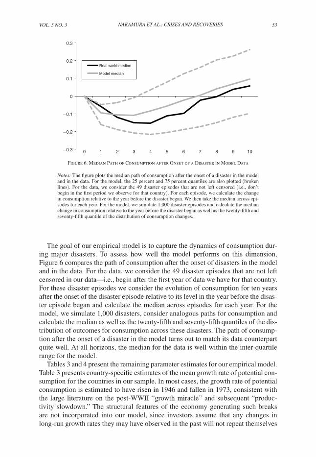
The goal of our empirical model is to capture the dynamics of consumption dur-ing major disasters. To assess how well the model performs on this dimension, Figure 6 compares the path of consumption after the onset of disasters in the model and in the data. For the data, we consider the 49 disaster episodes that are not left censored in our data—i.e., begin after the first year of data we have for that country. For these disaster episodes we consider the evolution of consumption for ten years after the onset of the disaster episode relative to its level in the year before the disas-ter episode began and calculate the median across episodes for each year. For the model, we simulate 1,000 disasters, consider analogous paths for consumption and calculate the median as well as the twenty-fifth and seventy-fifth quantiles of the dis-tribution of outcomes for consumption across these disasters. The path of consump-tion after the onset of a disaster in the model turns out to match its data counterpart quite well. At all horizons, the median for the data is well within the inter-quartile range for the model.
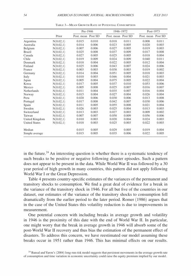
Tables 3 and 4 present the remaining parameter estimates for our empirical model. Table 3 presents country-specific estimates of the mean growth rate of potential con-sumption for the countries in our sample. In most cases, the growth rate of potential consumption is estimated to have risen in 1946 and fallen in 1973, consistent with the large literature on the post-WWII “growth miracle” and subsequent “produc-tivity slowdown.” The structural features of the economy generating such breaks are not incorporated into our model, since investors assume that any changes in long-run growth rates they may have observed in the past will not repeat themselves
−0.3
−0.2
−0.1
0
0.1
0.2
0.3
0 1 2 3 4 5 6 7 8 9 10
Real world median
Model median
Figure 6. Median Path of Consumption after Onset of a Disaster in Model Data
notes: The figure plots the median path of consumption after the onset of a disaster in the model and in the data. For the model, the 25 percent and 75 percent quantiles are also plotted (broken lines). For the data, we consider the 49 disaster episodes that are not left censored (i.e., don’t begin in the first period we observe for that country). For each episode, we calculate the change in consumption relative to the year before the disaster began. We then take the median across epi-sodes for each year. For the model, we simulate 1,000 disaster episodes and calculate the median change in consumption relative to the year before the disaster began as well as the twenty-fifth and seventy-fifth quantile of the distribution of consumption changes.
54 AMErIcAn EcOnOMIc JOurnAL: MAcrOEcOnOMIcs JuLy 2013
in the future.24 An interesting question is whether there is a systematic tendency of such breaks to be positive or negative following disaster episodes. Such a pattern does not appear to be present in the data. While World War II was followed by a 30 year period of high growth in many countries, this pattern did not apply following World War I or the Great Depression.
Table 4 presents country-specific estimates of the variances of the permanent and transitory shocks to consumption. We find a great deal of evidence for a break in the variance of the transitory shock in 1946. For all but five of the countries in our dataset, our estimates of the variance of the transitory shocks to consumption fell dramatically from the earlier period to the later period. Romer (1986) argues that in the case of the United States this volatility reduction is due to improvements in measurement.
One potential concern with including breaks in average growth and volatility in 1946 is the proximity of this date with the end of World War II. In particular, one might worry that the break in average growth in 1946 will absorb some of the post-World War II recovery and thus bias the estimation of the permanent effect of disasters. To address this concern, we have reestimated our model assuming these breaks occur in 1951 rather than 1946. This has minimal effects on our results.
24 Bansal and Yaron’s (2004) long-run risk model suggests that persistent movements in the average growth rate of consumption and time variation in economic uncertainty could raise the equity premium implied by our model.
Table 3—Mean Growth Rate of Potential Consumption
Prior
Pre-1946 1946–1972 Post-1973
Post. mean Post SD Post. mean Post SD Post. mean Post SD
Argentina N(0.02,1) 0.015 0.010 0.018 0.011 0.008 0.011Australia N(0.02,1) 0.014 0.006 0.023 0.005 0.020 0.003Belgium N(0.02,1) 0.007 0.006 0.027 0.005 0.019 0.003Brazil N(0.02,1) 0.025 0.008 0.037 0.009 0.017 0.008Canada N(0.02,1) 0.027 0.005 0.025 0.005 0.018 0.004Chile N(0.02,1) 0.019 0.009 0.024 0.009 0.040 0.011Denmark N(0.02,1) 0.018 0.004 0.022 0.005 0.012 0.004Finland N(0.02,1) 0.025 0.006 0.043 0.007 0.024 0.006France N(0.02,1) 0.003 0.003 0.038 0.003 0.019 0.002Germany N(0.02,1) 0.014 0.004 0.051 0.005 0.018 0.003Italy N(0.02,1) 0.010 0.003 0.046 0.004 0.021 0.003Japan N(0.02,1) 0.005 0.004 0.075 0.005 0.022 0.004Korea N(0.02,1) 0.017 0.005 0.037 0.010 0.053 0.006Mexico N(0.02,1) 0.005 0.008 0.025 0.007 0.016 0.007Netherlands N(0.02,1) 0.011 0.004 0.035 0.007 0.016 0.004Norway N(0.02,1) 0.015 0.004 0.027 0.004 0.026 0.004Peru N(0.02,1) 0.020 0.006 0.030 0.006 0.013 0.008Portugal N(0.02,1) 0.017 0.008 0.042 0.007 0.030 0.006Spain N(0.02,1) 0.011 0.005 0.055 0.008 0.021 0.004Sweden N(0.02,1) 0.026 0.003 0.025 0.004 0.013 0.003Switzerland N(0.02,1) 0.013 0.003 0.027 0.003 0.009 0.002Taiwan N(0.02,1) 0.007 0.007 0.058 0.009 0.056 0.006United Kingdom N(0.02,1) 0.010 0.003 0.020 0.004 0.024 0.003United States N(0.02,1) 0.018 0.003 0.025 0.003 0.022 0.003
Median 0.015 0.005 0.029 0.005 0.019 0.004Simple average 0.015 0.005 0.035 0.006 0.022 0.005

VOL. 5 nO. 3 55Nakamura et al.: Crises aNd reCoveries
The short-run disaster shock is slightly larger, while the long-run disaster shock is somewhat smaller. This version generates asset pricing results that are quite similar to our baseline case (the CRRA required to hit the equity premium rises from 6.4 to 6.8). We report detailed results for this version of the model in online Appendix B.
For robustness, we have estimated an alternative specification of our model in which we assume that ϕ i, t , the short-run disaster shock, has a gamma distribution. Results for this specification are presented in Table 5. Most of the estimates are similar to the baseline case. The main difference is that the gamma model assigns a somewhat larger portion of the volatility of consumption during disasters to the short-run shock as opposed to the long-run shock.
Table 5—Disaster Parameters with Gamma Shocks
Prior dist. Prior mean Prior SD Post. mean Post SD
p W Uniform 0.050 0.029 0.035 0.017 p cbW Uniform 0.500 0.289 0.715 0.094 p cbI Uniform 0.050 0.029 0.008 0.0041− p ce Uniform 0.500 0.289 0.847 0.029 ρ z Uniform 0.450 0.260 0.541 0.037ϕ Uniform 0.100 0.058 0.075 0.011θ Normal 0.000 0.200 −0.020 0.006 σ ϕ Uniform 0.130 0.069 0.091 0.008 σ θ Uniform 0.130 0.069 0.110 0.012
Table 4—Standard Deviation of Nondisaster Shocks
Priors Permanent Temporary Pre-1946 Temporary Post-1946
Post. mean Post SD Post. mean Post SD Post. mean Post SD
Argentina U[0,0.15] 0.053 0.009 0.020 0.013 0.013 0.009Australia U[0,0.15] 0.017 0.004 0.036 0.008 0.004 0.003Belgium U[0,0.15] 0.020 0.002 0.013 0.009 0.003 0.002Brazil U[0,0.15] 0.047 0.006 0.062 0.011 0.010 0.007Canada U[0,0.15] 0.024 0.003 0.026 0.009 0.003 0.002Chile U[0,0.15] 0.043 0.009 0.038 0.018 0.018 0.010Denmark U[0,0.15] 0.021 0.003 0.005 0.004 0.005 0.003Finland U[0,0.15] 0.031 0.005 0.020 0.008 0.004 0.003France U[0,0.15] 0.014 0.002 0.031 0.005 0.002 0.001Germany U[0,0.15] 0.019 0.002 0.011 0.006 0.002 0.002Italy U[0,0.15] 0.019 0.002 0.011 0.003 0.003 0.002Japan U[0,0.15] 0.022 0.003 0.017 0.005 0.003 0.002Korea U[0,0.15] 0.026 0.004 0.027 0.007 0.004 0.003Mexico U[0,0.15] 0.036 0.004 0.034 0.008 0.005 0.004Netherlands U[0,0.15] 0.023 0.003 0.017 0.006 0.003 0.002Norway U[0,0.15] 0.022 0.002 0.004 0.003 0.004 0.003Peru U[0,0.15] 0.033 0.004 0.007 0.005 0.004 0.003Portugal U[0,0.15] 0.033 0.004 0.023 0.008 0.005 0.003Spain U[0,0.15] 0.024 0.003 0.045 0.008 0.003 0.002Sweden U[0,0.15] 0.019 0.002 0.020 0.004 0.003 0.002Switzerland U[0,0.15] 0.012 0.001 0.039 0.005 0.002 0.001Taiwan U[0,0.15] 0.033 0.004 0.018 0.016 0.004 0.003United Kingdom U[0,0.15] 0.018 0.002 0.003 0.002 0.003 0.002United States U[0,0.15] 0.018 0.002 0.021 0.004 0.003 0.002
Median 0.023 0.003 0.020 0.006 0.003 0.002Simple average 0.026 0.004 0.023 0.007 0.005 0.003
56 AMErIcAn EcOnOMIc JOurnAL: MAcrOEcOnOMIcs JuLy 2013
V. Asset Pricing
We follow Mehra and Prescott (1985) in analyzing the asset-pricing implications of the consumption process we estimate in section IV within the context of a rep-resentative consumer endowment economy. We assume that the representative con-sumer in our model has preferences of the type developed by Epstein and Zin (1989) and Weil (1990). For this preference specification, Epstein and Zin (1989) show that the return on an arbitrary cash flow is given by the solution to the following equation:
(4) E t [ β ξ ( c i, t+1 _
c i, t )
(−ξ/ψ) r w, i, t+1
−(1−ξ) r j, i, t+1 ] = 1,
where r j, i, t+1 denotes the gross return on an arbitrary asset j in country i from period t to period t + 1, and r w, i, t+1 denotes the gross return on wealth of the representative agent in country i, which in our model equals the endowment stream. The parameter β represents the subjective discount factor of the representative
consumer. The parameter ξ = 1−γ _
1−1/ψ , where γ is the coefficient of relative risk
aversion (CRRA), and ψ is the intertemporal elasticity of substitution (IES), which governs the agent’s desire to smooth consumption over time.25
The asset-pricing implications of our model with Epstein-Zin-Weil (EZW) prefer-ences cannot be derived analytically. We therefore use standard numerical methods.26 We begin by calculating returns for two assets: a one period risk-free bill and an unlev-eraged claim on the consumption process. In Section VC, we calculate asset prices for a long-term bond and allow for partial default on bills and bonds during disasters.
Barro and Ursúa (2008a) report rates of return for stocks, bonds and bills for 17 countries over long periods (see Table 5 of their paper). The average arithmetic real rate of return on stocks is 8.1 percent per year, while the average arithmetic real rate of return on short-term bills is 0.9 percent per year. The average equity premium is therefore 7.2 percent per year. If we view stock returns as a levered claim on the consumption stream, the target equity premium for an unleveraged claim on the con-sumption stream is lower than that for stocks. According to the Federal Reserve’s Flow-of-Funds Accounts for recent years, the debt-equity ratio for US nonfinancial
25 The representative-consumer approach that we adopt abstracts from heterogeneity across consumers. Wilson (1968) and Constantinides (1982) show that a heterogeneous-consumer economy is isomorphic to a representative-consumer economy if markets are complete and agents have expected utility preferences. See also Rubinstein (1974). Constantinides and Duffie (1996) argue that highly persistent, heteroscedastic, uninsurable income shocks can resolve the equity premium puzzle.
26 We solve the integral in equation (4) on a grid. Specifically, we start by solving for the price-dividend ratio for a consumption claim. In this case we can rewrite equation (4) as PD r t c = E t [ f ( Δ c t+1 , PD r t+1 c
) ] , where PD r t c denotes the price dividend ratio of the consumption claim. We specify a grid for PD r t c over the state space. We then solve numerically for a fixed point for PD r t c as a function of the state of the economy on the grid. We can then rewrite equation (4) for other assets as PD r t = E t [ f ( Δ c t+1 , Δ D t+1 , PD r t+1 c
, PD r t+1 ) ] , where PD r t denotes the price dividend ratio of the asset in question and Δ D t+1 denotes the growth rate of its dividend. Given that we have already solved for PD r t c , we can solve numerically for a fixed point for PD r t for any other asset as a function of the state of the economy on the grid. This approach is similar to the one used by Campbell and Cochrane (1999) and Wachter (forthcoming).
VOL. 5 nO. 3 57Nakamura et al.: Crises aNd reCoveries
corporations is roughly one-half. This amount of leverage implies that the target equity premium for an unleveraged consumption claim in our model should be 4.8 percent per year (7.2/1.5).27 We therefore take 4.8 percent per year as the target for the equity premium in our analysis.
To analyze the asset-pricing implications of our model we must choose values for the CRRA, γ; the IES, ψ; and the discount factor, β. There is little agreement within the macroeconomics and finance literature about the appropriate value for the IES. Hall (1988) estimates the IES to be close to zero. This estimate is obtained by analyzing the response of aggregate consumption growth to movements in the real interest rate over time. Yet, as noted by Bansal and Yaron (2004) and Gruber (2006), the interest rate and consumption growth result from capital-market equilibrium, making it difficult to estimate the causal effect of one on the other without strong structural assumptions. These concerns are sometimes addressed by using lagged interest rates as instruments for movements in the current interest rate. However, this instrumentation strategy is successful only if there are no slowly moving parameters of preferences and technology (including especially parameters related to uncer-tainty) that affect interest rates and consumption growth. Alternative procedures for identifying exogenous variation in the interest rate sometimes generate much larger estimates of the IES. For example, Gruber (2006) uses instruments based on cross-state variation in tax rates on capital income to estimate a value close to 2 for the IES. As a consequence, a wide variety of parameter values for the IES are used in the asset-pricing literature. On the one hand, Campbell (2003) and Guvenen (2009) advocate values for the IES well below 1, while Bansal and Yaron (2004) use a value of the IES of 1.5 and Barro (2009) relies on Gruber (2006) to use a value of 2. We argue below that low values of the IES are starkly inconsistent with the observed behavior of asset prices during consumption disasters. We therefore focus on param-eterizations with an IES equal to two— ψ = 2—as our baseline case.
We present results for several different values of the CRRA. Our baseline value of the CRRA is chosen to match the equity premium in the data. Differences in the discount factor β have only minimal effects on the equity premium in our model.28 They do, however, affect the risk-free rate. We choose the discount factor β to match the risk-free rate in the data for our baseline values for γ and ψ. This procedure yields a value of β = exp(−0.034).
The consumption data we analyze reflect any international risk sharing that agents may have engaged in. The asset-pricing equations we use are standard Euler equations involving domestic consumption and domestic asset returns. In pr inciple, we could also investigate the asset-pricing implications of Euler equations that link domestic consumption, foreign consumption, and the exchange rate (see, e.g., Backus and Smith 1993). A large literature in international finance explores how the form that these Euler equations take depends on the structure of international financial
27 Dividing the equity premium for levered equity by one plus the debt-equity ratio to get a target for unlev-eraged equity is exact in the simple disaster model of Barro (2006). A concern with this approach in our case is that firms may have an incentive to default during disasters. We abstract from this issue. Abel (1999) argues for approximating levered equity by a scaled consumption claim. Bansal and Yaron (2004) and others have adopted this approach. For our model, the two approaches yield virtually indistinguishable results.
28 In the continuous time limit of our discrete time model, the equity premium is unaffected by β.

58 AMErIcAn EcOnOMIc JOurnAL: MAcrOEcOnOMIcs JuLy 2013
markets. Analyzing these issues is beyond the scope of this paper. However, recent work suggests that rare disasters may help to explain anomalies in the be havior of the real exchange rate.29
A. The Equity Premium with Epstein-Zin-Weil Preferences
Table 6 presents our main results regarding the equity premium. The equity pre-mium is reported for three cases: our baseline model as estimated in Section IV, a version of our model without disasters as in Mehra and Prescott (1985), and a version of the model in which disasters are permanent and occur in a single period as in Barro (2006).30 The statistics we report are the logarithm of the arithmetic average gross return on each asset ( log E [ r j, i, t+1 ] ) . These calculations are based on the posterior means of the parameters of our model.31 We discuss sampling uncertainty below.
Our estimated model matches the observed equity premium given a CRRA of 6.4. For this CRRA, the model yields an equity premium about ten times larger than the model without disasters. The model without disaster risk implies essentially no equity premium, in line with Mehra and Prescott (1985). Our analysis shows, therefore, that even accounting for the partially transitory nature of disasters, and the fact that they unfold over multiple years, disaster risk greatly amplifies the equity premium. On the other hand, the model with permanent, one-period disasters of the type analyzed in Barro (2006) yields an equity premium roughly ten times larger than our estimated model. Our analysis, thus, also shows that ignoring recoveries and the multi-year nature of disasters greatly overstates their asset-pricing implica-tions. Given the close link between the equity premium and the welfare costs of economic fluctuations (Alvarez and Jermann 2004; Barro 2009), these differences imply that our model yields costs of economic fluctuations substantially larger than a model that ignores disaster risk, but substantially smaller than the Rietz-Barro model of permanent and instantaneous disasters.
29 Papers on this topic include Bates (1996); Brunnermeier, Nagel, and Pedersen (2009); Burnside et al. (2008); Farhi et al. (2009); Farhi and Gabaix (2008); Guo (2007); and Jurek (2008).
30 For the model without disasters, we set the probability of entering a disaster to zero. For the model with permanent, one-period disasters, we set the probability of exiting a disaster equal to one, assume that ϕ i, t = θ i, t , and that the distribution of these shocks corresponds to the distribution of the peak-to-trough drop in consumption over the course of disasters in our baseline model.
31 For the parameters σ ϵ, i, t 2 and μ i, t , we use the values for the post-1946 and post-1973 periods, respectively. And
we assume that agents view these parameters as being fixed.
Table 6—Disasters and the Equity Premium
Equity premium Risk-free rate
Baseline 0.048 0.010No disasters 0.005 0.042Permanent, one period disasters 0.466 −0.378
notes: All cases have CRRA = 6.4, IES = 2, and β = exp(−0.034). The return statistics are the log of the average gross return for each asset. The “equity premium” is the difference between the average return on an unlevered equity claim and bills. The “risk-free rate” is the average return on bills. These results are produced by simulating a long sample from the model with a representative set of disasters.
VOL. 5 nO. 3 59Nakamura et al.: Crises aNd reCoveries
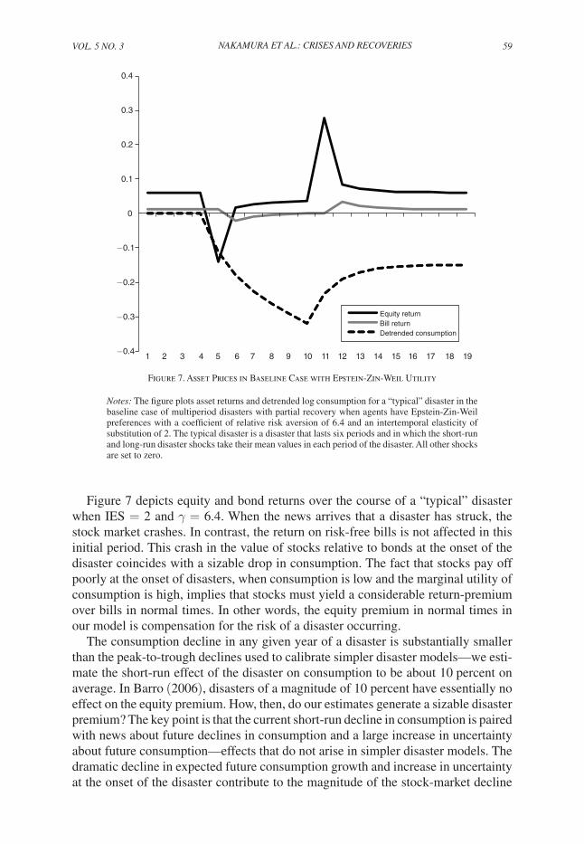
Figure 7 depicts equity and bond returns over the course of a “typical” disaster when IES = 2 and γ = 6.4. When the news arrives that a disaster has struck, the stock market crashes. In contrast, the return on risk-free bills is not affected in this initial period. This crash in the value of stocks relative to bonds at the onset of the disaster coincides with a sizable drop in consumption. The fact that stocks pay off poorly at the onset of disasters, when consumption is low and the marginal utility of consumption is high, implies that stocks must yield a considerable return-premium over bills in normal times. In other words, the equity premium in normal times in our model is compensation for the risk of a disaster occurring.
The consumption decline in any given year of a disaster is substantially smaller than the peak-to-trough declines used to calibrate simpler disaster models—we esti-mate the short-run effect of the disaster on consumption to be about 10 percent on average. In Barro (2006), disasters of a magnitude of 10 percent have essentially no effect on the equity premium. How, then, do our estimates generate a sizable disaster premium? The key point is that the current short-run decline in consumption is paired with news about future declines in consumption and a large increase in uncertainty about future consumption—effects that do not arise in simpler disaster models. The dramatic decline in expected future consumption growth and increase in uncertainty at the onset of the disaster contribute to the magnitude of the stock-market decline
−0.4
−0.3
−0.2
−0.1
0
0.1
0.2
0.3
0.4
Equity return
Bill return
Detrended consumption
1 2 3 4 5 6 7 8 9 10 11 12 13 14 15 16 17 18 19
Figure 7. Asset Prices in Baseline Case with Epstein-Zin-Weil Utility
notes: The figure plots asset returns and detrended log consumption for a “typical” disaster in the baseline case of multiperiod disasters with partial recovery when agents have Epstein- Zin-Weil preferences with a coefficient of relative risk aversion of 6.4 and an intertemporal elasticity of substitution of 2. The typical disaster is a disaster that lasts six periods and in which the short-run and long-run disaster shocks take their mean values in each period of the disaster. All other shocks are set to zero.
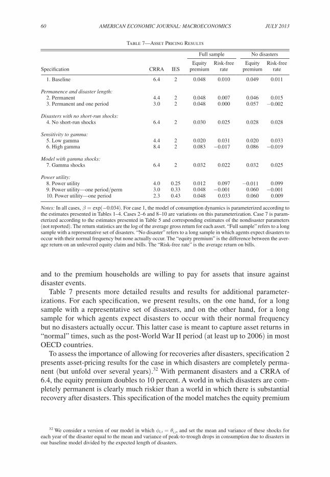
60 AMErIcAn EcOnOMIc JOurnAL: MAcrOEcOnOMIcs JuLy 2013
and to the premium households are willing to pay for assets that insure against disaster events.
Table 7 presents more detailed results and results for additional parameter-izations. For each specification, we present results, on the one hand, for a long sample with a representative set of disasters, and on the other hand, for a long sample for which agents expect disasters to occur with their normal frequency but no disasters actually occur. This latter case is meant to capture asset returns in “normal” times, such as the post-World War II period (at least up to 2006) in most OECD countries.
To assess the importance of allowing for recoveries after disasters, specification 2 presents asset-pricing results for the case in which disasters are completely perma-nent (but unfold over several years).32 With permanent disasters and a CRRA of 6.4, the equity premium doubles to 10 percent. A world in which disasters are com-pletely permanent is clearly much riskier than a world in which there is substantial recovery after disasters. This specification of the model matches the equity premium
32 We consider a version of our model in which ϕ i, t = θ i, t , and set the mean and variance of these shocks for each year of the disaster equal to the mean and variance of peak-to-trough drops in consumption due to disasters in our baseline model divided by the expected length of disasters.
Table 7—Asset Pricing Results
Specification CRRA IES
Full sample No disasters
Equity premium
Risk-free rate
Equity premium
Risk-free rate
1. Baseline 6.4 2 0.048 0.010 0.049 0.011
Permanence and disaster length: 2. Permanent 4.4 2 0.048 0.007 0.046 0.015 3. Permanent and one period 3.0 2 0.048 0.000 0.057 −0.002
Disasters with no short-run shocks: 4. No short-run shocks 6.4 2 0.030 0.025 0.028 0.028
sensitivity to gamma: 5. Low gamma 4.4 2 0.020 0.031 0.020 0.033 6. High gamma 8.4 2 0.083 −0.017 0.086 −0.019
Model with gamma shocks: 7. Gamma shocks 6.4 2 0.032 0.022 0.032 0.025
Power utility: 8. Power utility 4.0 0.25 0.012 0.097 −0.011 0.099 9. Power utility—one period/perm 3.0 0.33 0.048 −0.001 0.060 −0.001 10. Power utility—one period 2.3 0.43 0.048 0.033 0.060 0.009
notes: In all cases, β = exp(−0.034). For case 1, the model of consumption dynamics is parameterized according to the estimates presented in Tables 1–4. Cases 2–6 and 8–10 are variations on this parameterization. Case 7 is param-eterized according to the estimates presented in Table 5 and corresponding estimates of the nondisaster parameters (not reported). The return statistics are the log of the average gross return for each asset. “Full sample” refers to a long sample with a representative set of disasters. “No disaster” refers to a long sample in which agents expect disasters to occur with their normal frequency but none actually occur. The “equity premium” is the difference between the aver-age return on an unlevered equity claim and bills. The “Risk-free rate” is the average return on bills.

VOL. 5 nO. 3 61Nakamura et al.: Crises aNd reCoveries
in the data when the CRRA is set to 4.4.33 The fact that our model allows for partial recovery after disasters thus accounts for a large part of the difference in our results and the results of Barro (2006) and Barro and Ursúa (2008a).
To assess the role of the multi-period nature of disasters in our model, s pecification 3 presents results for a case in which the drop in consumption associ-ated with a disaster occurs in a single period, and the drop is permanent. With a CRRA of 6.4, this model yields an equity premium of 47 percent. We can match the equity premium in the data for this specification of the model with a CRRA of 3.0.34 This specification raises the equity premium because the stock market crash coincides perfectly with the trough in consumption—when the marginal utility of consumption is highest. In contrast, when disasters unfold over multiple periods, the stock market crash occurs at the onset of the disaster, while a large fraction of the drop in consumption occurs in subsequent periods. Also, if the drop in consumption associated with a disaster occurs in a single period, it does not lead to an increased desire to save. In multi-period disasters, expectations of further drops in consump-tion increase the desire to save. This response strengthens the demand for stocks, limiting the magnitude of the stock-market crash.
To assess the importance of the short-run drop in consumption during disasters, specification 4 presents results for a case in which the short-run disaster shocks are set to zero. In this specification, the occurrence of a disaster does not bring with it a sharp drop in consumption followed by a partial recovery. Rather, consumption falls gradually due to the long-run disaster shocks while the disaster persists. With a CRRA of 6.4, this specification yields an equity premium of 3.0 percent—about 60 percent of the equity premium in the benchmark specification. This shows that both the short-run and long-run effects of disasters on consumption are important for the equity premium.
An advantage of our formal estimation approach is that it allows us to investi-gate the strength of the statistical evidence for disaster risk as an explanation for the equity premium. Because they occur rarely, there is much less information on the frequency, size, and shape of disasters than on business-cycle phenomena. This perspective suggests that the statistical uncertainty regarding the estimates of the equity premium presented above may be large. The posterior distribution for the equity premium implied by the posterior distribution of the parameters of our model is plotted in Figure 8 for our baseline parameter values. Figure 8 shows that our esti-mates place more than 90 percent weight on parameter combinations that generate an equity premium of more than 3.3 percent. The centered 90 percent probability interval for the equity premium implied by the model is [3.0, 7.0] percent.
33 Notice that we lowered the CRRA by roughly 30 percent and this change leads to a drop in the equity pre-mium of about 50 percent. This pattern illustrates that the equity premium is highly convex in the CRRA in our model. Specifications 5 and 6 of Table 7 illustrate this point further.
34 The model analyzed in specification 3 is very similar to the model analyzed by Barro and Ursúa (2008a). Their model matches the equity premium when γ = 3.5, while the model in specification 3 matches the equity pre-mium for γ = 3.0. This difference arises because the size distribution of disasters in our model is relative to trend, while the peak-to-trough distribution used by Barro and Ursúa (2008a) does not adjust for trend growth over the course of the disaster and because of differences between our approach to estimating the distribution of disasters and the nonparametric approach used by Barro and Ursúa (2008a).

62 AMErIcAn EcOnOMIc JOurnAL: MAcrOEcOnOMIcs JuLy 2013
A different way of assessing this issue is to plot the posterior distribution of the value of the CRRA that matches the observed equity premium. This distribution is plotted in Figure 9.35 The centered 90 percent probability interval for the CRRA is [5.3, 7.8]. Thus, despite the limited data, the observed disasters provide substantial statistical evidence that it is possible to explain the observed equity premium with values of the CRRA less than ten.
To check that our results are not somehow “built in” to our priors or estimation algorithm, we analyze what our estimation algorithm implies for a dataset gener-ated from a model without disasters; that is, a setting similar to the one used by Mehra and Prescott (1985). In this counterfactual exercise, it is important that we allow ourselves only as many observations as we have in the data. We therefore simulate an artificial dataset of the same size as our data (24 countries and a total of 2,685 observations) from our model with the disaster probabilities set to 0. We then estimate our model on these data and calculate the posterior distribution of the equity premium. This distribution is plotted in Figure 10. For this alternative dataset, our model places a large probability on the equity premium being below 1 percent. These results are strikingly different from those implied by our estimated model (Figure 8), indicating that it is the data—not our priors or estimation algo-rithm—that lead us to the conclusion that the fear of rare disasters can explain a sizable equity premium.
35 For every parameter combination sampled from the estimated posterior distributions of the parameters, we calculate the value of the CRRA required to match the equity premium.
0.00 0.05 0.10 0.15
Equity premium
Den
sity
0
10
20
30
Figure 8. Posterior Distribution of the Equity Premium

VOL. 5 nO. 3 63Nakamura et al.: Crises aNd reCoveries
It is interesting to note in Figure 10 that while the majority of the mass is located close to zero, the distribution has a long right tail. This long, right tail implies that even if no disasters were observed in a sample the size of ours, agents would still place some weight on the notion that disasters occur with a nontrivial probability, and that the sample they had observed was simply not representative of the underly-ing process (a “Peso problem”).
For robustness, we also calculated asset-pricing results for the alternative specifica-tion of our model in which the short-run disaster shocks follow a Gamma distribution. This case yields similar asset pricing results, which are presented in specification 7 of Table 7. With γ = 6.4 and an IES of 2, the equity premium is 3.2 percent and the risk-free rate is 2.2 percent. The gamma model matches the equity premium and risk-free rate when γ = 7.7. This difference arises because the gamma model allo-cates slightly more of the overall volatility in consumption to the short-run shock than to the long-run shock, compared to the baseline model.
B. The Equity Premium with Power utility
Much work on asset pricing, including Mehra and Prescott (1985), Rietz (1988), and Barro (2006), considers the special case of power utility. In this case, the coef-ficient of relative risk aversion equals the reciprocal of the IES— γ = 1/ψ. In other words, a single parameter governs consumers’ willingness to bear risk and substi-tute consumption over time. Asset pricing results for our model with power utility
0 4 8 12
Gamma
Den
sity
0.0
0.1
0.6
0.6
0.6
0.3
0.2
1062
Figure 9. Distribution of the Coefficient of Relative Risk Aversion
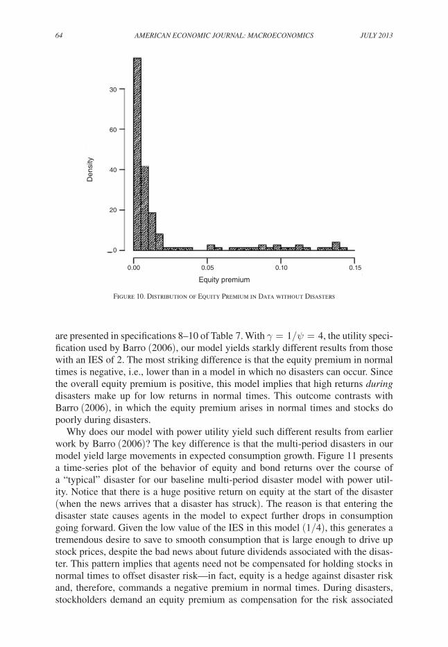
64 AMErIcAn EcOnOMIc JOurnAL: MAcrOEcOnOMIcs JuLy 2013
are presented in specifications 8–10 of Table 7. With γ = 1/ψ = 4, the utility speci-fication used by Barro (2006), our model yields starkly different results from those with an IES of 2. The most striking difference is that the equity premium in normal times is negative, i.e., lower than in a model in which no disasters can occur. Since the overall equity premium is positive, this model implies that high returns during disasters make up for low returns in normal times. This outcome contrasts with Barro (2006), in which the equity premium arises in normal times and stocks do poorly during disasters.
Why does our model with power utility yield such different results from earlier work by Barro (2006)? The key difference is that the multi-period disasters in our model yield large movements in expected consumption growth. Figure 11 presents a time-series plot of the behavior of equity and bond returns over the course of a “typical” disaster for our baseline multi-period disaster model with power util-ity. Notice that there is a huge positive return on equity at the start of the disaster (when the news arrives that a disaster has struck). The reason is that entering the disaster state causes agents in the model to expect further drops in consumption going forward. Given the low value of the IES in this model (1/4), this generates a tremendous desire to save to smooth consumption that is large enough to drive up stock prices, despite the bad news about future dividends associated with the disas-ter. This pattern implies that agents need not be compensated for holding stocks in normal times to offset disaster risk—in fact, equity is a hedge against disaster risk and, therefore, commands a negative premium in normal times. During disasters, stockholders demand an equity premium as compensation for the risk associated
0.00 0.05 0.10 0.15
Equity premium
Den
sity
0
40
60
30
20
Figure 10. Distribution of Equity Premium in Data without Disasters
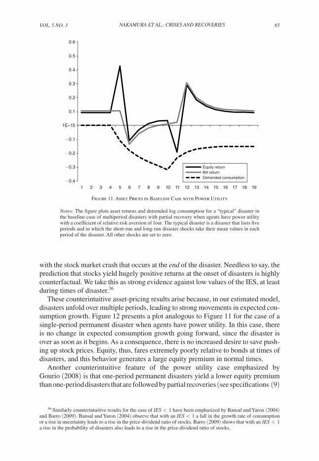
VOL. 5 nO. 3 65Nakamura et al.: Crises aNd reCoveries
with the stock market crash that occurs at the end of the disaster. Needless to say, the prediction that stocks yield hugely positive returns at the onset of disasters is highly counterfactual. We take this as strong evidence against low values of the IES, at least during times of disaster.36
These counterintuitive asset-pricing results arise because, in our estimated model, disasters unfold over multiple periods, leading to strong movements in expected con-sumption growth. Figure 12 presents a plot analogous to Figure 11 for the case of a single-period permanent disaster when agents have power utility. In this case, there is no change in expected consumption growth going forward, since the disaster is over as soon as it begins. As a consequence, there is no increased desire to save push-ing up stock prices. Equity, thus, fares extremely poorly relative to bonds at times of disasters, and this behavior generates a large equity premium in normal times.
Another counterintuitive feature of the power utility case emphasized by Gourio (2008) is that one-period permanent disasters yield a lower equity premium than one-period disasters that are followed by partial recoveries (see specifications (9)
36 Similarly counterintuitive results for the case of IEs < 1 have been emphasized by Bansal and Yaron (2004) and Barro (2009). Bansal and Yaron (2004) observe that with an IEs < 1 a fall in the growth rate of consumption or a rise in uncertainty leads to a rise in the price-dividend ratio of stocks. Barro (2009) shows that with an IEs < 1 a rise in the probability of disasters also leads to a rise in the price-dividend ratio of stocks.
−0.4
−0.3
−0.2
−0.1
1E–15
0.1
0.2
0.3
0.4
0.5
0.6
Equity return Bill returnDetrended consumption
1 2 3 4 5 6 7 8 9 10 11 12 13 14 15 16 17 18 19
Figure 11. Asset Prices in Baseline Case with Power Utility
notes: The figure plots asset returns and detrended log consumption for a “typical” disaster in the baseline case of multiperiod disasters with partial recovery when agents have power utility with a coefficient of relative risk aversion of four. The typical disaster is a disaster that lasts five periods and in which the short-run and long-run disaster shocks take their mean values in each period of the disaster. All other shocks are set to zero.
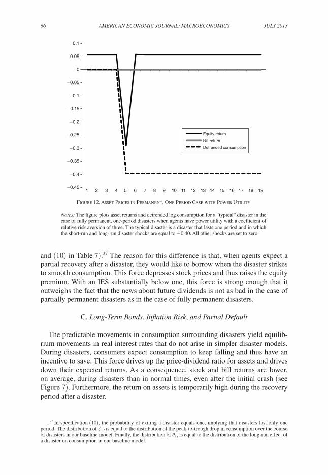
66 AMErIcAn EcOnOMIc JOurnAL: MAcrOEcOnOMIcs JuLy 2013
and (10) in Table 7).37 The reason for this difference is that, when agents expect a partial recovery after a disaster, they would like to borrow when the disaster strikes to smooth consumption. This force depresses stock prices and thus raises the equity premium. With an IES substantially below one, this force is strong enough that it outweighs the fact that the news about future dividends is not as bad in the case of partially permanent disasters as in the case of fully permanent disasters.
C. Long-Term Bonds, Inflation risk, and Partial Default
The predictable movements in consumption surrounding disasters yield equilib-rium movements in real interest rates that do not arise in simpler disaster models. During disasters, consumers expect consumption to keep falling and thus have an incentive to save. This force drives up the price-dividend ratio for assets and drives down their expected returns. As a consequence, stock and bill returns are lower, on average, during disasters than in normal times, even after the initial crash (see Figure 7). Furthermore, the return on assets is temporarily high during the recovery period after a disaster.
37 In specification (10), the probability of exiting a disaster equals one, implying that disasters last only one period. The distribution of ϕ i, t is equal to the distribution of the peak-to-trough drop in consumption over the course of disasters in our baseline model. Finally, the distribution of θ i, t is equal to the distribution of the long-run effect of a disaster on consumption in our baseline model.
−0.45
−0.4
−0.35
−0.3
−0.25
−0.2
−0.15
−0.1
−0.05
0
0.05
0.1
Equity return
Bill return Detrended consumption
1 2 3 4 5 6 7 8 9 10 11 12 13 14 15 16 17 18 19
Figure 12. Asset Prices in Permanent, One Period Case with Power Utility
notes: The figure plots asset returns and detrended log consumption for a “typical” disaster in the case of fully permanent, one-period disasters when agents have power utility with a coefficient of relative risk aversion of three. The typical disaster is a disaster that lasts one period and in which the short-run and long-run disaster shocks are equal to −0.40. All other shocks are set to zero.
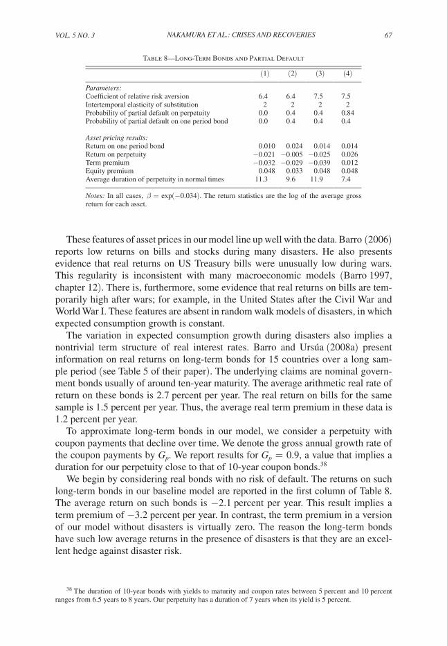
VOL. 5 nO. 3 67Nakamura et al.: Crises aNd reCoveries
These features of asset prices in our model line up well with the data. Barro (2006) reports low returns on bills and stocks during many disasters. He also presents evidence that real returns on US Treasury bills were unusually low during wars. This regularity is inconsistent with many macroeconomic models (Barro 1997, chapter 12). There is, furthermore, some evidence that real returns on bills are tem-porarily high after wars; for example, in the United States after the Civil War and World War I. These features are absent in random walk models of disasters, in which expected consumption growth is constant.
The variation in expected consumption growth during disasters also implies a nontrivial term structure of real interest rates. Barro and Ursúa (2008a) present information on real returns on long-term bonds for 15 countries over a long sam-ple period (see Table 5 of their paper). The underlying claims are nominal govern-ment bonds usually of around ten-year maturity. The average arithmetic real rate of return on these bonds is 2.7 percent per year. The real return on bills for the same sample is 1.5 percent per year. Thus, the average real term premium in these data is 1.2 p ercent per year.
To approximate long-term bonds in our model, we consider a perpetuity with coupon payments that decline over time. We denote the gross annual growth rate of the coupon payments by G p . We report results for G p = 0.9, a value that implies a duration for our perpetuity close to that of 10-year coupon bonds.38
We begin by considering real bonds with no risk of default. The returns on such long-term bonds in our baseline model are reported in the first column of Table 8. The average return on such bonds is −2.1 percent per year. This result implies a term premium of −3.2 percent per year. In contrast, the term premium in a version of our model without disasters is virtually zero. The reason the long-term bonds have such low average returns in the presence of disasters is that they are an excel-lent hedge against disaster risk.
38 The duration of 10-year bonds with yields to maturity and coupon rates between 5 percent and 10 percent ranges from 6.5 years to 8 years. Our perpetuity has a duration of 7 years when its yield is 5 percent.
Table 8—Long-Term Bonds and Partial Default
(1) (2) (3) (4)
Parameters:Coefficient of relative risk aversion 6.4 6.4 7.5 7.5Intertemporal elasticity of substitution 2 2 2 2Probability of partial default on perpetuity 0.0 0.4 0.4 0.84Probability of partial default on one period bond 0.0 0.4 0.4 0.4
Asset pricing results:Return on one period bond 0.010 0.024 0.014 0.014Return on perpetuity −0.021 −0.005 −0.025 0.026Term premium −0.032 −0.029 −0.039 0.012Equity premium 0.048 0.033 0.048 0.048Average duration of perpetuity in normal times 11.3 9.6 11.9 7.4
notes: In all cases, β = exp(−0.034). The return statistics are the log of the average gross return for each asset.

68 AMErIcAn EcOnOMIc JOurnAL: MAcrOEcOnOMIcs JuLy 2013
To understand why the long bond is a valuable hedge against disasters, it is use-ful to compare it to stocks. When a disaster occurs, stocks are affected in two ways. First, the disaster is a negative shock to future expected dividends. This effect tends to depress stock prices. Second, the representative consumer has an increased desire to save, which tends to raise stock prices. With an IES = 2, the first effect dominates the second one, and stocks decline in value at the beginning of a disaster. The dif-ference between a long-term bond and stocks is that the coupon payments on the bonds are not affected by the disaster. The only effect that the disaster has on the long-term bond is therefore to raise its price because of consumers’ increased desire to save. Since the price of long-term bonds rises at the onset of a disaster, these bonds provide a hedge against disaster risk and earn a lower rate of return than bills in normal times.
A potentially important feature of the data that we have so far left out of our model is the possibility of partial default on nominal bonds. While literal default on bills is rare, even during disasters, inflation may lead to partial default on bills, particularly during disasters. To calibrate the probability of partial default, we fol-low Barro and Ursúa (2009a) in considering peak-to-trough drops in stock prices over time periods that correspond roughly to consumption disasters. Extending their empirical asset-price calculations to bills, we find that in 74 percent of the larg-est consumption disasters—25 cases out of 34—stock returns are lower than bill returns.39 The average stock return in these 25 cases is −34 percent, while the aver-age bill return is −3 percent. In the remaining 9 cases, the real return on stocks and bonds are similar. In these cases, the low real returns on bills (and bonds) are caused by huge amounts of inflation. These cases also tend to be ones in which the measure-ment of the timing of returns is most suspect because of market closure and controls on goods and asset prices.
These calculations suggest that an appropriate calibration of the probability of partial default is 26 percent (9/34). To be conservative, we set the probability of partial default to 40 percent, as in Barro (2006). The second and third columns of Table 8 report results for calibrations that allow for partial default on bills. For a CRRA of 6.4, this modification lowers the equity premium from 4.8 percent to 3.3 percent. Raising the CRRA to 7.5 restores the equity premium to 4.8 percent.
The news that a disaster has struck may affect the returns on long-term bonds more than the returns on bills if it raises inflationary expectations without leading to an immediate jump in the price level. This is one possible reason for the positive term premium on long-term nominal bonds in the data. We can match this term premium by raising the probability of partial default on long-term bonds rela-tive to short-term bonds. The fourth column in Table 8 reports results for a case in which the probability of partial default on the perpetuity is 84 percent, while the probability of partial default on short-term bonds is 40 percent. For these
39 Here we identify disasters as events in which the peak-to-trough drop in consumption is larger than 17 p ercent. We choose this cutoff because applying it to the data yields a set of events that corresponds closely to the disaster episodes identified by our model. For the subset of countries that we use to estimate our model, we get 48 events as compared to 53 disaster episodes identified by our model. The average drop in consumption for these events is 32 percent, compared to 29 percent for our disaster episodes. There are 34 events for which we have data on both stock and bill returns.
VOL. 5 nO. 3 69Nakamura et al.: Crises aNd reCoveries
probabilities of partial default, our model matches the term premium on nominal bonds in the data.
Our model implies that, without default risk on bonds, the term structure is down-ward sloping, but introducing partial default can match the observed upward-slop-ing term structure for nominal bonds. If most of the default risk comes from inflation risk, our model implies that the term structure for real bonds should be less upward sloping or even downward sloping. In the United Kingdom, a large and liquid mar-ket for indexed government bonds has existed for several decades. Piazzesi and Schneider (2007) document that while the UK nominal yield curve has been upward sloping, the real yield curve has been downward sloping. In the United States, indexed bonds (TIPS) have been trading since 1997. Piazzesi and Schneider (2007)document that the TIPS curve over this period appears to be mostly upward slop-ing, contrary to our prediction. They caution, however, that this evidence is hard to assess because of the short sample and poor liquidity in the TIPS market.40
D. Additional Predictions
Recent work by van Binsbergen, Brandt, and Koijen (2012) and Binsbergen et al. (2011) has shown that short-term dividend strips on the aggregate stock market have substantially higher expected returns than the stock market as a whole.41 They point out that this fact is difficult to match using leading equilibrium asset-pricing models, such as Campbell and Cochrane (1999), Bansal and Yaron (2004), and Barro (2006). In contrast, this feature arises naturally in our model. For the baseline calibration of our model, a 1-year dividend strip on unleveraged equity—i.e., an asset that pays off a single dividend equal to consumption in the next period—has a return premium of 13.7 percent over bills outside of disasters, compared to an unleveraged equity premium of 4.9 percent for the stock market as a whole. This pattern reflects the presence of recoveries in our model, which raise the riskiness of short-term assets relative to long-term assets.42
Our model is related, in general terms, to other explanations for the equity pre-mium in which predictable movements in consumption play an important role. A leading example is the long-run risks model of Bansal and Yaron (2004). However, one important difference between our model and theirs is that, while consumption growth is highly predictable during disasters and in the periods immediately follow-ing disasters, we do not require that it be predictable in other periods. Since disasters occur infrequently, the explanatory power of the price-dividend ratio in predicting future consumption growth at medium and short horizons is close to zero in our
40 See also Evans (1998), Barr and Campbell (1997), and Campbell, Shiller, and Viceira (2009).41 The price of a k-year dividend strip is the present value of the dividend paid in k years.42 Lettau and Wachter (2007) present a model in which long-horizon assets are less risky than short-horizon
assets. A key feature of their model—like ours—is that negative shocks to dividends are associated with increases in expected dividend growth. Lettau and Wachter posit an exogenous stochastic discount factor that generates important asset pricing implications of these shocks for the cross-section of expected returns and use asset-price data to calibrate its parameters. In our model, the stochastic discount factor is derived from the utility function of the representative consumer and the dynamics of consumption. Our model therefore provides evidence of an important role for these shocks based on consumption data alone.
70 AMErIcAn EcOnOMIc JOurnAL: MAcrOEcOnOMIcs JuLy 2013
model.43 In contrast, the long-run risks model generates substantial forecastability of consumption growth using the price-dividend ratio. Beeler and Campbell (2012) argue that this feature of the model is hard to reconcile with US consumption data, particularly in the post-World War II period.
The analysis of this section suggests that variation in expected consumption growth surrounding disasters has important implications for asset pricing. It is nevertheless useful to ask what parameters would best approximate our estimated c onsumption process in the simpler random walk framework studied by Rietz (1988) and Barro (2006). The equity premium in the random-walk model is
log E r e − log r f = γ σ 2 + pE{b[(1 − b ) −γ − 1]},
where p denotes the probability of disasters, b denotes the permanent instantaneous fraction by which consumption drops at the time of disasters, σ 2 denotes the variance of consumption growth in normal times, and γ denotes the coefficient of relative risk aversion. Fixing the probability of disasters at our empirical estimate of 2.8 percent, we can replicate our baseline equity premium results in the random-walk model with a fixed disaster size of b = 0.27.44 This value of b is substantially smaller than in the parameterizations implied by Barro (2006) and Barro and Ursúa (2008a) where the risk-adjusted disaster size is roughly 0.4.45 The smaller “effective” size of disasters implied by our estimates arises from the importance of recoveries and multi-period disasters.
VI. Conclusion
We estimate a quantitative model of consumption disasters that allows for recov-eries, and for disasters to unfold over multiple periods. We find strong evidence for both of these features. Allowing for recoveries implies less risk associated with disasters, lowering the equity premium for given risk aversion. Allowing disasters to unfold over multiple periods implies strongly predictable movements in consump-tion, which also leads to a reduction in the equity premium. Even accounting for these features of the data, and for the statistical uncertainty arising from the rare nature of disasters, disaster risk greatly amplifies the equity premium.
Our estimated model matches the observed equity premium given a coefficient of relative risk aversion (CRRA) of 6.4, with a centered 90 percent probability interval of [5.3, 7.8]. For these parameters, a Mehra-Prescott type model that ignores disas-ter risk implies an equity premium close to zero. On the other hand, the Rietz-Barro model yields an equity premium more than ten times as large as our benchmark
43 Specifically, we have analyzed regressions of consumption growth at one-, three-, and five-year horizons on the current price dividend ratios. The r 2 of such regressions is consistently 3 percent or less.
44 Specifically, this is the value of b that matches the observed equity premium for our baseline estimate of risk aversion of γ = 6.4 and disaster probability p = 2.8 percent.
45 Both Barro (2006) and Barro and Ursúa (2008a) study models with a distribution of disaster sizes. However, it is possible to solve for the value of b that matches their equity premium results for a given value of p and γ. Barro and Ursúa (2008a) analyze a model with a disaster probability of 0.0363 and γ = 3.5, implying that the equity premium results can be replicated with b = 0.4. Barro’s (2006) calibration assumes a disaster probability of 0.017 and γ = 4, implying that b = 0.36 is required to fit the equity premium.
VOL. 5 nO. 3 71Nakamura et al.: Crises aNd reCoveries
model. These conclusions are robust to the inclusion of empirically realistic amounts of default risk on government bonds.
The predictable movements in consumption growth we estimate surrounding disasters imply that the intertemporal elasticity of substitution plays a more impor-tant role than in simpler disaster models. At the onset of a disaster, agents expect steep future declines in consumption, implying a strong desire to save. If the inter-temporal elasticity of substitution is low, stock prices will counterfactually boom at the onset of disasters. This counterfactual prediction provides evidence against low values of the IES at least during times of disaster. The predictable movements in consumption we estimate also yield equilibrium movements in interest rates, a non-trivial term structure of interest rates, and predictions for dividend strips on stocks that line up well with recent empirical estimates.
A concern for tractability has required us to make a number of simplifying assumptions when specifying our empirical model. For example, we assume that the short-run and long-run disaster shocks are uncorrelated. In reality, these may be positively correlated. We also abstract from any correlation in the size of contem-poraneous disasters across countries and our specification for the correlation in the timing of disasters is very simple (e.g., abstracts from geographical variation and autocorrelation). Also, we do not incorporate time variation in growth and uncer-tainty during normal times. Nakamura, Sergeyev, and Steinsson (2012) estimate a model that incorporates these last two features and find that they have important asset pricing implications. As computational costs continue to fall, we hope that future research will be able to relax more of these assumptions.
An interesting extension of our approach would be to estimate a model of time-variation in disaster probabilities. Aside from variation in the actual probability of disasters, the perceived disaster probability may vary due to learning. Even condi-tioning on all the available time-series data, our estimates suggest there is substan-tial uncertainty regarding the disaster parameter, implying that learning may play an important role. Variation in disaster probabilities, whether real or perceived, have the potential to generate significant volatility of asset returns—an important feature of the asset pricing data.
REFERENCES
Abel, Andrew B. 1999. “Risk premia and term premia in general equilibrium.” Journal of Monetary Economics 43 (1): 3–33.
Alvarez, Fernando, and Urban J. Jermann. 2004. “Using Asset Prices to Measure the Cost of Business Cycles.” Journal of Political Economy 112 (6): 1223–56.
Arakelian, Veni, and Efthymios G. Tsionas. 2009. “Bayesian Analysis of the Consumption CAPM.” In Advances in Econometrics, Vol. 23, edited by Thomas B. Fomby, R. Carter Hill, Ivan Jeliazkov, and Juan Carlos, 619–43. Bingley, UK: Emerald.
Backus, David K., and Gregor W. Smith. 1993. “Consumption and real exchange rates in dynamic economies with non-traded goods.” Journal of International Economics 35 (3–4): 297–316.
Balke, Nathan S., and Robert J. Gordon. 1989. “The Estimation of Prewar Gross National Product: Methodology and New Evidence.” Journal of Political Economy 97 (1): 38–92.
Bansal, Ravi, and Amir Yaron. 2004. “Risks for the Long Run: A Potential Resolution of Asset Pricing Puzzles.” Journal of Finance 59 (4): 1481–1509.
Barr, D. G., and John Y. Campbell. 1997. “Inflation, real interest rates, and the bond market: A study of UK nominal and index-linked government bond prices.” Journal of Monetary Economics 39 (1): 361–83.
72 AMErIcAn EcOnOMIc JOurnAL: MAcrOEcOnOMIcs JuLy 2013
Barro, Robert J. 1997. Macroeconomics. Cambridge, MA: MIT Press.Barro, Robert J. 2006. “Rare Disasters and Asset Markets in the Twentieth Century.” Quarterly Jour-
nal of Economics 121 (3): 832–66.Barro, Robert J. 2009. “Rare Disasters, Asset Prices, and Welfare Costs.” American Economic review
99 (1): 243–64.Barro, Robert J., and Tao Jin. 2011. “On the Size Distribution of Macroeconomic Disasters.” Econo-
metrica 79 (5): 1567–89.Barro, Robert J., and José F. Ursúa. 2008a. “Macroeconomic Crises since 1870.” Brookings Papers on
Economic Activity 38 (1): 255–350.Barro, Robert J., and José F. Ursúa. 2008b. “Macroeconomic Crises since 1870: Dataset.” Brookings
Papers on Economic Activity. http://rbarro.com/data-sets/ (accessed June 2008).Barro, Robert J., and José F. Ursúa. 2009a. “Stock-Market Crashes and Depressions.” National Bureau
of Economic Research (NBER) Working Paper 14760.Barro, Robert J., and José F. Ursúa. 2009b. “Stock-Market Crashes and Depressions: Dataset.”
(accessed September 2009).Bates, David S. 1996. “Jumps and Stochastic Volatility: Exchange Rate Processes Implicit in Deutsche
Mark Options.” review of Financial studies 9 (1): 69–107.Beeler, Jason, and John Y. Campbell. 2012. “The Long-Run Risk Model and Aggregate Asset Prices:
An Empirical Assessment.” critical Finance review 1 (1): 141–82.van Binsbergen, Jules, Michael Brandt, and Ralph Koijen. 2012. “On the Timing and Pricing of Divi-
dends.” American Economic review 102 (4): 1596–1618.van Binsbergen, Jules H., Wouter H. Hueskes, Ralph S. J. Koijen, and Evert B. Vrugt. 2011. “Equity
Yields.” National Buruea of Economic Research (NBER) Working Paper 17416.Brunnermeier, Markus K., Stefan Nagel, and Lasse H. Pedersen. 2009. “Carry Trades and Currency
Crashes.” In nBEr Macroeconomics Annual 2008, Vol. 23, edited by Daron Acemoglu, Kenneth Rogoff, and Michael Woodford, 313–47. Chicago: University of Chicago Press.
Burnside, Craig, Martin Eichenbaum, Isaac Kleshchelski, and Sergio Rebelo. 2008. “Do Peso Prob-lems Explain the Returns to the Carry Trade?” review of Financial studies 24 (3): 853–91.
Campbell, John Y. 2003. “Consumption-Based Asset Pricing.” In Handbook of the Economics of Finance, Vol. 1B, edited by George M. Constantinides, Milton Harris, and René M. Stulz, 802–87. Amsterdam: Elsevier.
Campbell, John Y., and John H. Cochrane. 1999. “By Force of Habit: A Consumption-Based Explana-tion of Aggregate Stock Market Behavior.” Journal of Political Economy 107 (2): 205–51.
Campbell, John Y., Robert J. Shiller, and Luis M. Viceira. 2009. “Understanding Inflation-Indexed Bond Markets.” Brooking Papers on Economic Activity 39 (1): 79–120.
Cerra, Valerie, and Sweta Chaman Saxena. 2008. “Growth Dynamics: The Myth of Economic Recov-ery.” American Economic review 98 (1): 439–57.
Cochrane, John H. 1988. “How Big Is the Random Walk in GNP?” Journal of Political Economy 96 (5): 893–920.
Cogley, Timothy. 1990. “International Evidence on the Size of the Random Walk in Output.” Journal of Political Economy 98 (3): 501–18.
Constantinides, George. 1982. “Intertemporal Asset Pricing with Heterogeneous Consumers and with-out Demand Aggregation.” Journal of Business 55 (2): 253–67.
Constantinides, George M. 2008. “Macroeconomic Crises since 1870: Comment.” Brookings Papers on Economic Activity 38 (1): 341–49.
Constantinides, George M., and Darrell Duffie. 1996. “Asset Pricing with Heterogeneous Consumers.” Journal of Political Economy 104 (2): 219–40.
Davis, Donald R., and David E. Weinstein. 2002. “Bones, Bombs and Break Points: The Geography of Economic Activity.” American Economic review 92 (5): 1269–89.
Dimson, Elroy, Paul Marsh, and Mike Staunton. 2002. Triumph of the Optimists. Princeton: Princeton University Press.
Epstein, Larry G., and Stanley E. Zin. 1989. “Substitution, Risk Aversion and the Temporal Behavior of Consumption and Asset Returns.” Econometrica 57 (4): 937–69.
Eraker, Bjørn, Michael Johannes, and Nicholas Polson. 2003. “The Impact of Jumps in Volatility and Returns.” Journal of Finance 58 (3): 1269–1300.
Evans, Martin D. D. 1998. “Real Rates, Expected Inflation, and Inflation Risk Premia.” Journal of Finance 53 (1): 187–218.
Farhi, Emmanuel, Samuel P. Fraiberger, Xavier Gabaix, Romain Ranciere, and Adrien Verdel-han. 2009. “Crash Risk in Currency Markets.” http://papers.ssrn.com/sol3/Delivery.cfm/SSRN_ID1412883_code368958.pdf?abstractid=1397668&mirid=1.

VOL. 5 nO. 3 73Nakamura et al.: Crises aNd reCoveries
Farhi, Emmanuel, and Xavier Gabaix. 2008. “Rare Disasters and Exchange Rates.” http://federation.ens.fr/ydepot/semin/texte0809/GAB2008RAR.pdf.
Gabaix, Xavier. 2008. “Variable Rare Disasters: A Tractable Theory of Ten Puzzles in Macro-Finance.” American Economic review 98 (2): 64–67.
Gelfand, Alan E. 2000. “Gibbs Sampling.” Journal of the American statistical Association 95 (452): 1300–1304.
Gelman, Andrew, John B. Carlin, Hal S. Stern, and Donald B. Rubin. 2004. Bayesian Data Analysis. Boca Raton: Chapman and Hall.
Gelman, Andrew, and Donald B. Rubin. 1992. “Inference from Iterative Simulation Using Multiple Sequences.” statistical science 7 (4): 457–511.
Geweke, John. 2005. contemporary Bayesian Econometrics and statistics. Hoboken: John Wiley and Sons.
Geweke, John. 2007. “Models, Computational Experiments and Reality.” http://papers.ssrn.com/sol3/Delivery.cfm/SSRN_ID1009603_code31584.pdf?abstractid=1009603&mirid=1.
Gourio, François. 2008. “Disasters and Recoveries.” American Economic review 98 (2): 68–73.Gourio, François. 2012. “Disaster Risk and Business Cycles.” American Economic review 102 (6):
2734–66.Gruber, Jonathan. 2006. “A Tax-Based Estimate of the Elasticity of Intertemporal Substitution.”
National Bureau of Economic Research (NBER) Working Paper 11945.Guo, Kai. 2007. “Exchange Rates and Asset Prices in an Open Economy with Rare Disasters.” http://
www.dallasfed.org/assets/documents/institute/events/2008/080324guo.pdf.Guvenen, Fatih. 2009. “A Parsimonious Macroeconomic Model for Asset Pricing.” Econometrica 77
(6): 1711–50.Hall, Robert E. 1988. “Intertemporal Substitution in Consumption.” Journal of Political Economy 96
(2): 339–57.Hansen, Lars Peter, and Kenneth J. Singleton. 1982. “Generalized Instrumental Variables Estimation
of Nonlinear Rational Expectations Models.” Econometrica 50 (5): 1269–88.Julliard, Christian, and Anisha Ghosh. 2012. “Can Rare Events Explain the Equity Premium Puzzle?”
review of Financial studies 25 (10): 3037–76.Jurek, Jakob W. 2008. “Crash-Neutral Currency Carry Trades.” http://www.ssc.wisc.edu/~cengel/
Econ872/Jurek.pdf.Kilian, Lutz, and Lee E. Ohanian. 2002. “Unit Roots, Trend Breaks, and Transitory Dynamics: A Mac-
roeconomic Perspective.” Macroeconomic Dynamics 6 (5): 614–32.Koop, Gary, and Simon M. Potter. 2007. “Estimation and Forecasting in Models with Multiple Breaks.”
review of Economic studies 74 (3): 763–89.Lettau, Martin, and Jessica A. Wachter. 2007. “Why Is Long-Horizon Equity Less Risky? A Duration-
Based Explanation of the Value Premium.” Journal of Finance 62 (1): 55–92.Lucas, Robert E., Jr. 1978. “Asset Prices in an Exchange Economy.” Econometrica 46 (6): 1429–45.Maddison, Angus. 2003. The World Economy: Historical statistics. Paris: OECD Development Centre.Martin, Ian W. R. 2008. “Disasters and the Welfare Cost of Uncertainty.” American Economic review
98 (2): 74–78.Mehra, Rajnish, and Edward C. Prescott. 1985. “The Equity Premium: A Puzzle.” Journal of Mon-
etary Economics 15 (2): 145–61.Nakamura, Emi, Dmitriy Sergeyev, and Jon Steinsson. 2012. “Growth-Rate and Uncertainty Shocks in
Consumption: Cross-Country Evidence.” http://www.columbia.edu/~en2198/papers/longrunrisk.pdf.
Nakamura, Emi, Jón Steinsson, Robert Barro, and José Ursúa. 2013. “Crises and Recoveries in an Empirical Model of Consumption Disasters: Dataset.” American Economic Journal: Macroeco-nomics. http://dx.doi.org/10.1257/mac.5.3.35.
Perron, Pierre. 1989. “The Great Crash, the Oil Price Shock, and the Unit Root Hypothesis.” Econo-metrica 57 (6): 1361–1401.
Pesaran, M. Hashem, Davide Pettenuzzo, and Allan Timmermann. 2006. “Forecasting Time Series Subject to Multiple Structural Breaks.” review of Economic studies 73 (4): 1057–84.
Piazzesi, Monika. 2010. “Understanding Returns on Average and over Time.” nBEr reporter: Asset Pricing Program report 2010 (2): 1–7. http://www.nber.org/reporter/2010number2/2010no2.pdf.
Piazzesi, Monika, and Martin Schneider. 2007. “Equilibrium Yield Curves.” In nBEr Macroeconom-ics Annual 2006, Vol. 21, edited by Daron Acemoglu, Kenneth Rogoff, and Michael Woodford, 389–442. Cambridge, MA: MIT Press.
Rietz, Thomas A. 1988. “The Equity Risk Premium: A Solution.” Journal of Monetary Economics 22 (1): 117–31.
74 AMErIcAn EcOnOMIc JOurnAL: MAcrOEcOnOMIcs JuLy 2013
Romer, Christina D. 1986. “Is the Stabilization of the Postwar Economy a Figment of the Data?” American Economic review 76 (3): 314–34.
Rubinstein, Mark. 1974. “An aggregation theorem for securities markets.” Journal of Financial Eco-nomics 1 (3): 225–44.
Smith, A. F. M., and A. E. Gelfand. 1992. “Bayesian Statistics Without Tears: A Sampling-Resampling Perspective.” American statistician 46 (2): 84–88.
Tsionas, Efthymios G. 2005. “Likelihood Evidence on the Asset Returns Puzzle.” review of Economic studies 72 (3): 917–46.
Wachter, Jessica A. Forthcoming. “Can Time-Varying Risk of Rare Disasters Explain Aggregate Stock Market Volatility.” Journal of Finance.
Weil, Phillipe. 1990. “Nonexpected Utility in Macroeconomics.” Quarterly Journal of Economics 105 (1): 29–42.
Wilson, Robert B. 1968. “The Theory of Syndicates.” Econometrica 36 (1): 119–32.