crippling of thin-walled composite sections using...

AM-CONF13-43

Copyright © 2013 by Lockheed Martin Corporation.

Crippling of Thin-Walled Composite Sections using Progressive Failure Analysis

Scott Malaznik

Senior Staff Engineer

Lockheed Martin Aeronautics Company, Palmdale, California 93599

Summary

Aircraft structures, both metallic and composite, are often stiffened with thin-walled sections of

various shapes to resist compression loads efficiently. Analysis of these structures can be

challenging, and empirical methods are often used for design purposes. Since initial buckling is

not necessarily indicative of structural failure, the analysis must be carried into the post-buckling

range, where geometric and material nonlinearities are present. Final failure in this context is

called crippling, which corresponds to the maximum load carried by the section.

In this paper, the nonlinear capabilities of MSC Nastran SOL 400 are used to perform post-

buckling analysis of graphite/epoxy composite I-section stiffeners. After performing an

eigenvalue buckling analysis, initial imperfections in the shape of the buckling modes are applied

to the model to start the large displacement analysis. Composite material failures are modeled

using the Progressive Failure Analysis (PFA) feature of SOL 400. Results are plotted as load-

displacement curves, and crippling failure is defined as the maximum load carried. Results are

compared to published test data as well as MIL-HDBK-17 design equations.

Introduction

Thin-walled sections, composed of either metallic or composite materials, are commonly used in

the design of aircraft structures. Thin sections are prone to buckling, rather than material,

failures under compression loads, and therefore buckling analysis is of major importance in the

structural design of aircraft. It is well known that the initial buckling of thin walled structures

does not necessarily result in immediate failure, and this inherent post-buckling capability can be

used to achieve light weight designs. Indeed, recognition of the post-buckling load carrying

capability of metal structures helped make possible the transition from wood to metal aircraft

structures that occurred in the 1930s.

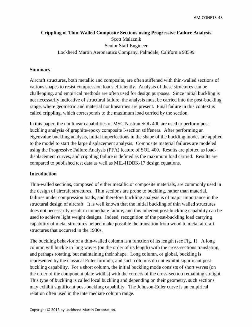
The buckling behavior of a thin-walled column is a function of its length (see Fig. 1). A long

column will buckle in long waves (on the order of its length) with the cross-sections translating,

and perhaps rotating, but maintaining their shape. Long column, or global, buckling is

represented by the classical Euler formula, and such columns do not exhibit significant post-

buckling capability. For a short column, the initial buckling mode consists of short waves (on

the order of the component plate widths) with the corners of the cross-section remaining straight.

This type of buckling is called local buckling and depending on their geometry, such sections

may exhibit significant post-buckling capability. The Johnson-Euler curve is an empirical

relation often used in the intermediate column range.


An abbreviated description of the post-buckling behavior of thin plates is given here to provide

background for this study. Detailed discussions can be found in many sources (for example, see

Ref. 1). When a thin flat rectangular plate supported on all edges buckles under axial

compression, the plate bends out of its initial plane. If the plate is visualized as a collection of

strips parallel to the load direction, it can be seen that after buckling the strips near the edges

remain nearly flat, while the curvature of the strips increases towards the middle. The axial

stiffness of these strips is a function of their curvature, with flatter strips being stiffer and more

curved strips being less stiff. Therefore, the stiffness distribution varies across the width of the

plate. This gives rise to the characteristic cosine distribution of stresses across the plate width.

Fig. 1 Column buckling behavior as a function of length

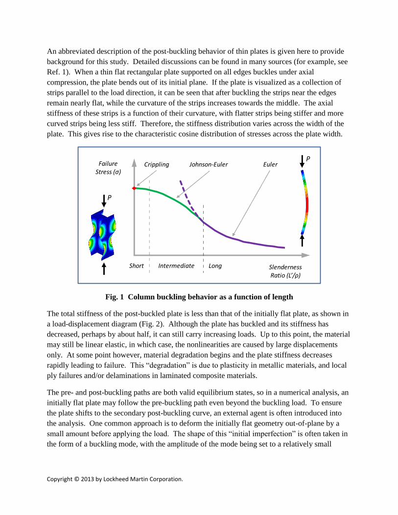
The total stiffness of the post-buckled plate is less than that of the initially flat plate, as shown in

a load-displacement diagram (Fig. 2). Although the plate has buckled and its stiffness has

decreased, perhaps by about half, it can still carry increasing loads. Up to this point, the material

may still be linear elastic, in which case, the nonlinearities are caused by large displacements

only. At some point however, material degradation begins and the plate stiffness decreases

rapidly leading to failure. This “degradation” is due to plasticity in metallic materials, and local

ply failures and/or delaminations in laminated composite materials.

The pre- and post-buckling paths are both valid equilibrium states, so in a numerical analysis, an

initially flat plate may follow the pre-buckling path even beyond the buckling load. To ensure

the plate shifts to the secondary post-buckling curve, an external agent is often introduced into

the analysis. One common approach is to deform the initially flat geometry out-of-plane by a

small amount before applying the load. The shape of this “initial imperfection” is often taken in

the form of a buckling mode, with the amplitude of the mode being set to a relatively small

LongShort Intermediate

EulerJohnson-EulerCrippling

Slenderness Ratio (L’/ρ)

Failure Stress (σ)

P

P


value, perhaps 0.1 to 0.5 times the plate thickness. This geometric imperfection can be viewed

as representing unavoidable small deviations from flatness of a real plate.

Due to the geometric and material nonlinearities involved in crippling failures, empirical

methods are usually used in the design of aircraft structures. Methodology for crippling of

metals was developed in the 1930s and is well documented in NACA-TN-3784 (Ref. 2). An

analogous approach for composites was developed in the 1970s and is documented in MIL-

HDBK-17 (Ref. 3). Refer to these documents for details on the available empirical crippling

prediction methodologies.

Fig. 2 Typical load-displacement behavior of a thin plate

Approach

The purpose of this study was to assess the applicability of the Progressive Failure Analysis

feature of MSC Nastran SOL 400 to crippling analysis of thin-walled composite sections. For

expediency, the geometry and material used in this study were selected to match those of Ref. 4,

so that the analysis results could be compared to the test data of that paper. Although Ref. 4

considered various cross sections, only one was considered here: an I-section with the

dimensions shown in Fig. 3a. As typical for crippling tests, the member lengths were short

enough to avoid column buckling and ensure local buckling modes were critical. Also, the

flange width is large relative to the web height so that local buckling of the flange is expected to

occur first. Four different lengths were analyzed (4, 6, 8, and 12 inches) but test data was only

available in Ref. 4 for two of the lengths (4 and 8 inches).

Axial Displacement (u)

AxialLoad (P)

Onset of material degradation

Initial Buckling

Final FailurePcc

Pcr


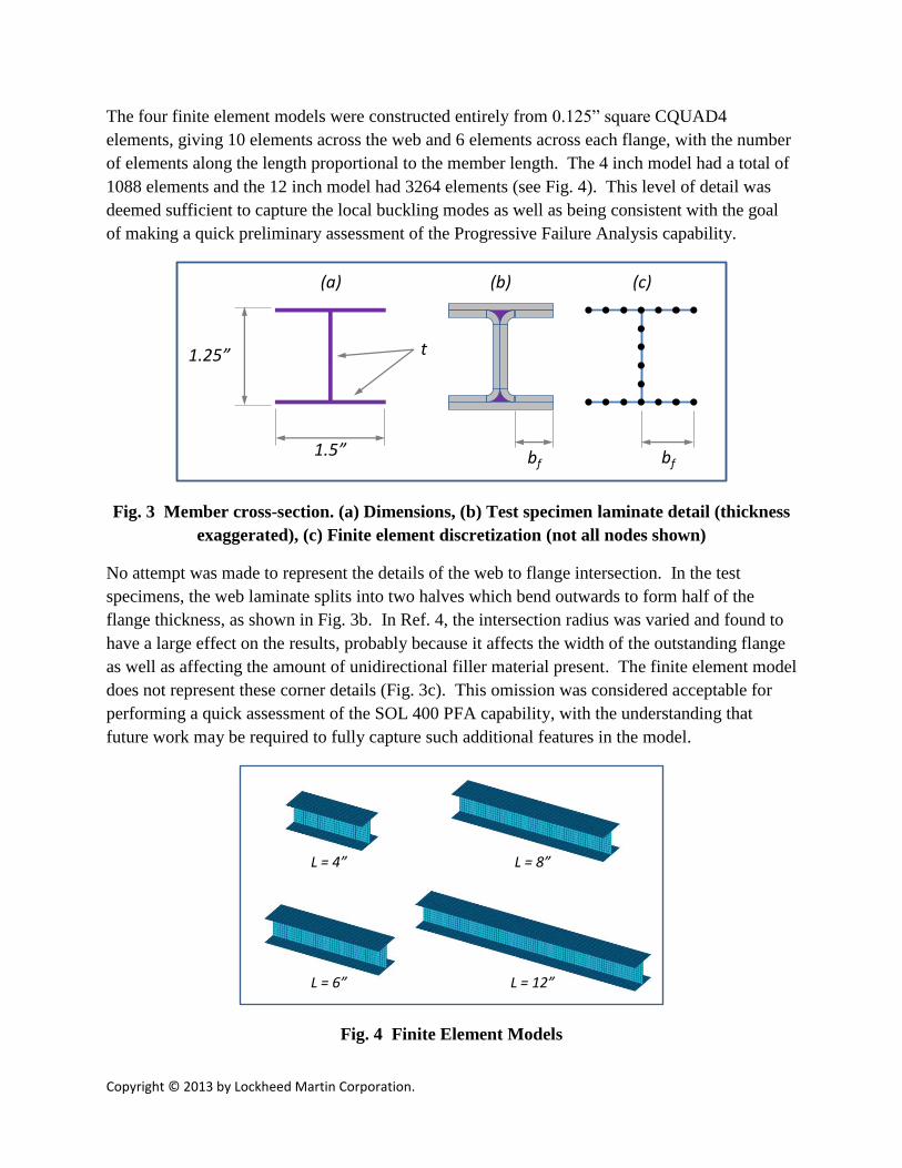
The four finite element models were constructed entirely from 0.125” square CQUAD4

elements, giving 10 elements across the web and 6 elements across each flange, with the number

of elements along the length proportional to the member length. The 4 inch model had a total of

1088 elements and the 12 inch model had 3264 elements (see Fig. 4). This level of detail was

deemed sufficient to capture the local buckling modes as well as being consistent with the goal

of making a quick preliminary assessment of the Progressive Failure Analysis capability.

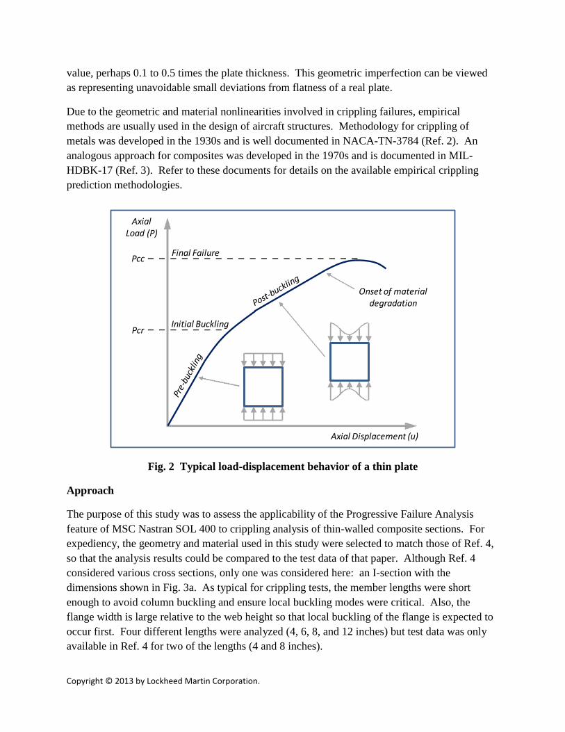
Fig. 3 Member cross-section. (a) Dimensions, (b) Test specimen laminate detail (thickness

exaggerated), (c) Finite element discretization (not all nodes shown)

No attempt was made to represent the details of the web to flange intersection. In the test

specimens, the web laminate splits into two halves which bend outwards to form half of the

flange thickness, as shown in Fig. 3b. In Ref. 4, the intersection radius was varied and found to

have a large effect on the results, probably because it affects the width of the outstanding flange

as well as affecting the amount of unidirectional filler material present. The finite element model

does not represent these corner details (Fig. 3c). This omission was considered acceptable for

performing a quick assessment of the SOL 400 PFA capability, with the understanding that

future work may be required to fully capture such additional features in the model.

Fig. 4 Finite Element Models

1.25”

1.5”

t

(a) (b) (c)

bf bf

L = 4” L = 8”

L = 6” L = 12”


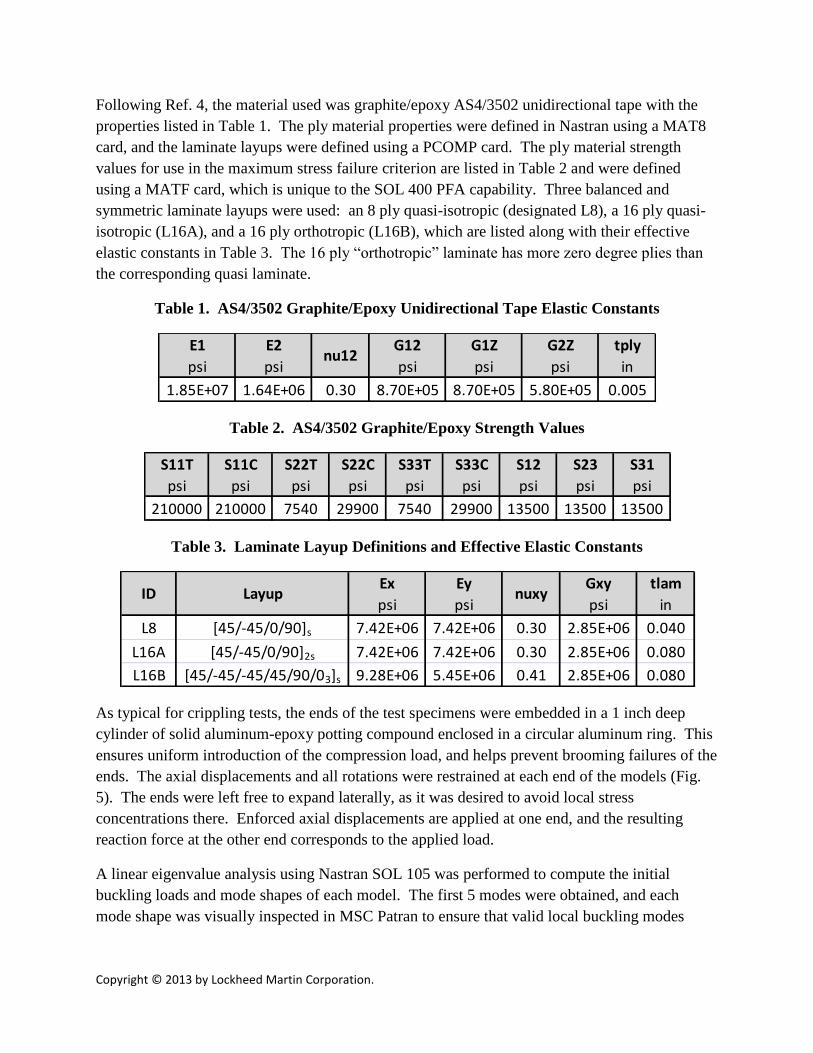
Following Ref. 4, the material used was graphite/epoxy AS4/3502 unidirectional tape with the

properties listed in Table 1. The ply material properties were defined in Nastran using a MAT8

card, and the laminate layups were defined using a PCOMP card. The ply material strength

values for use in the maximum stress failure criterion are listed in Table 2 and were defined

using a MATF card, which is unique to the SOL 400 PFA capability. Three balanced and

symmetric laminate layups were used: an 8 ply quasi-isotropic (designated L8), a 16 ply quasi-

isotropic (L16A), and a 16 ply orthotropic (L16B), which are listed along with their effective

elastic constants in Table 3. The 16 ply “orthotropic” laminate has more zero degree plies than

the corresponding quasi laminate.

Table 1. AS4/3502 Graphite/Epoxy Unidirectional Tape Elastic Constants

Table 2. AS4/3502 Graphite/Epoxy Strength Values

Table 3. Laminate Layup Definitions and Effective Elastic Constants

As typical for crippling tests, the ends of the test specimens were embedded in a 1 inch deep

cylinder of solid aluminum-epoxy potting compound enclosed in a circular aluminum ring. This

ensures uniform introduction of the compression load, and helps prevent brooming failures of the

ends. The axial displacements and all rotations were restrained at each end of the models (Fig.

5). The ends were left free to expand laterally, as it was desired to avoid local stress

concentrations there. Enforced axial displacements are applied at one end, and the resulting

reaction force at the other end corresponds to the applied load.

A linear eigenvalue analysis using Nastran SOL 105 was performed to compute the initial

buckling loads and mode shapes of each model. The first 5 modes were obtained, and each

mode shape was visually inspected in MSC Patran to ensure that valid local buckling modes

E1 E2 G12 G1Z G2Z tply

psi psi psi psi psi in

1.85E+07 1.64E+06 0.30 8.70E+05 8.70E+05 5.80E+05 0.005

nu12

S11T S11C S22T S22C S33T S33C S12 S23 S31

psi psi psi psi psi psi psi psi psi

210000 210000 7540 29900 7540 29900 13500 13500 13500

Ex Ey Gxy tlam

psi psi psi in

L8 [45/-45/0/90]s 7.42E+06 7.42E+06 0.30 2.85E+06 0.040

L16A [45/-45/0/90]2s 7.42E+06 7.42E+06 0.30 2.85E+06 0.080

L16B [45/-45/-45/45/90/03]s 9.28E+06 5.45E+06 0.41 2.85E+06 0.080

nuxyID Layup


occurred. The magnitude and location of the maximum out-of-plane flange displacement was

noted for later use in defining the initial geometric imperfections, as discussed next.

Fig. 5 Finite Element Model Boundary Conditions

To ensure that the cross section web and flange plates follow the post-buckling path rather than

remain flat, the initial geometry of the mesh was slightly deformed. The shape of the

imperfection was defined using a selected buckling mode shape, which was scaled so that the

maximum deformation was equal to a desired small value (see Fig. 6). For most of the analyses,

the first buckling mode was used as the imperfection shape and the amplitude was set to 0.02

inches, which was one-half of the thickness of the 8 ply laminate. For comparison, several runs

were made using other imperfection magnitudes and a few were made using the second buckling

mode as the imperfection shape. The Patran “Results/Results/Combine” utility was used to

offset the original nodes to the slightly deformed configuration.

Fig. 6 Definition of Initial Geometric Imperfection

Enforced Axial Displacement

P

u

Ends free to expand laterally

Imperfection Amplitude

Blue = PerfectRed = Imperfect


Using the slightly deformed geometry as the starting point, nonlinear analysis was performed

using Nastran SOL 400, including large displacements and composite material failure using

Progressive Failure Analysis. The LGDISP parameter was used to activate large displacements,

and a MATF card was used to define the material failure parameters. Default values were used

for most of the other nonlinear analysis parameters, such as those controlling load stepping,

stiffness updates, and convergence tolerances.

The PFA methodology offers several options for composite material failure criteria, including

maximum stress, maximum strain, Hill, Hoffman, Tsai-Wu, Hashin, and Puck (see the Nastran

Quick Reference Guide, Ref. 5). Some criteria require parameters which may not be readily

available for a given material. The maximum stress criterion was used exclusively in this study,

using the ply strength values listed in Table 2 (Ref. 4). This criterion was selected because the

required strength parameters were readily available, and not necessarily because it was thought

to be the most accurate option.

In the PFA methodology, once initial damage is identified by the selected failure criterion, the

ply stiffnesses are degraded according to the type of failure found. The rate of degradation can

be selected as immediate or gradual, and all results reported here used the gradual option. The

degraded material properties are used to re-compute the element stiffnesses, and the load

stepping then continues. The stiffness changes due to local damage cause load re-distribution

between different parts of the member. When enough elements have failed locally, the global

stiffness of the member starts to decrease. Final failure occurs when the stiffness drops to zero

and the member cannot carry additional load.

Buckling Analysis

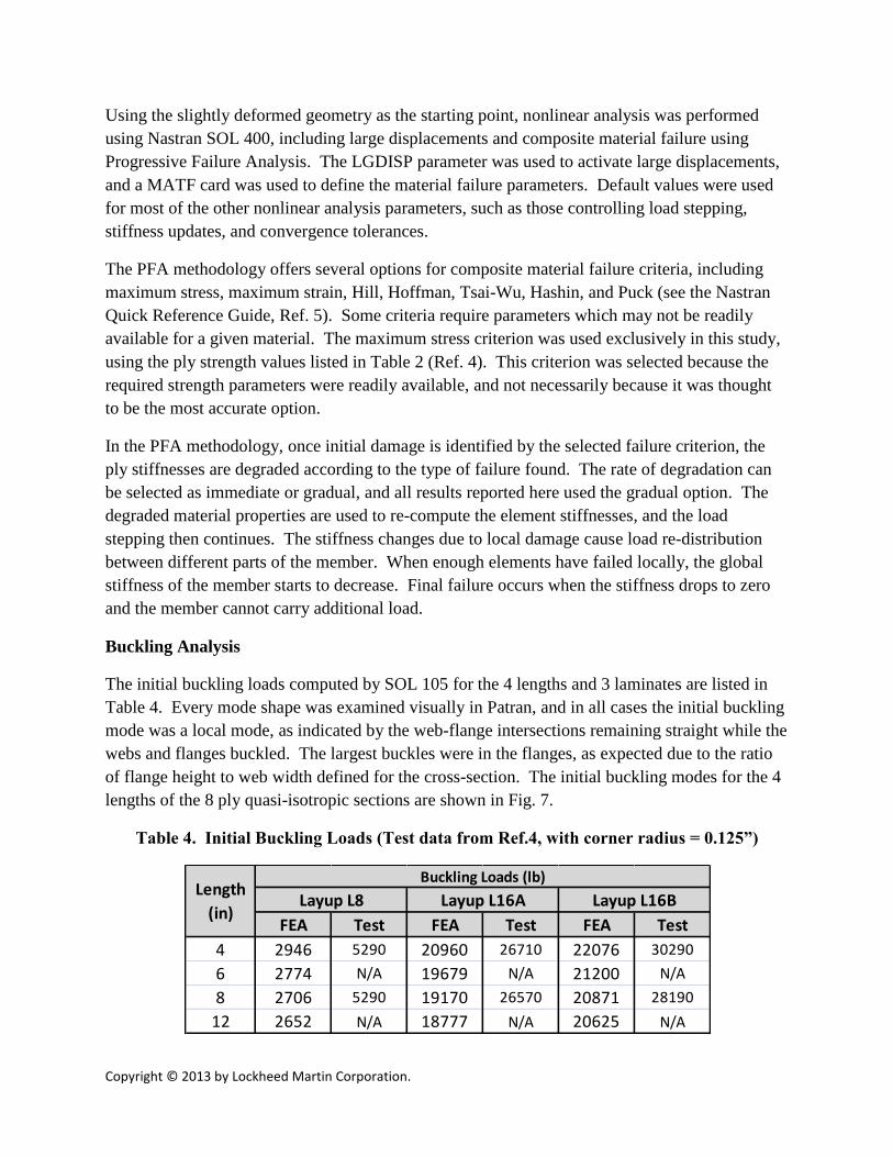
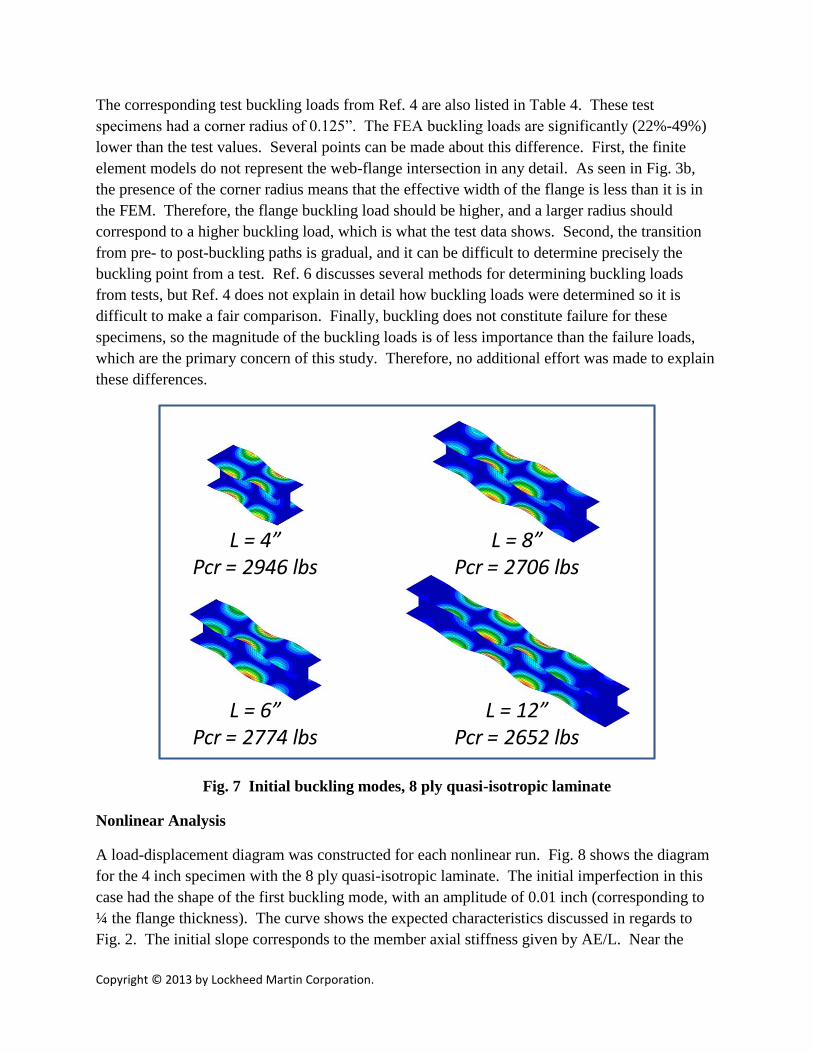
The initial buckling loads computed by SOL 105 for the 4 lengths and 3 laminates are listed in

Table 4. Every mode shape was examined visually in Patran, and in all cases the initial buckling

mode was a local mode, as indicated by the web-flange intersections remaining straight while the

webs and flanges buckled. The largest buckles were in the flanges, as expected due to the ratio

of flange height to web width defined for the cross-section. The initial buckling modes for the 4

lengths of the 8 ply quasi-isotropic sections are shown in Fig. 7.

Table 4. Initial Buckling Loads (Test data from Ref.4, with corner radius = 0.125”)

FEA Test FEA Test FEA Test

4 2946 5290 20960 26710 22076 30290

6 2774 N/A 19679 N/A 21200 N/A

8 2706 5290 19170 26570 20871 28190

12 2652 N/A 18777 N/A 20625 N/A

Layup L16BLayup L16ALayup L8

Buckling Loads (lb)Length

(in)


The corresponding test buckling loads from Ref. 4 are also listed in Table 4. These test

specimens had a corner radius of 0.125”. The FEA buckling loads are significantly (22%-49%)

lower than the test values. Several points can be made about this difference. First, the finite

element models do not represent the web-flange intersection in any detail. As seen in Fig. 3b,

the presence of the corner radius means that the effective width of the flange is less than it is in

the FEM. Therefore, the flange buckling load should be higher, and a larger radius should

correspond to a higher buckling load, which is what the test data shows. Second, the transition

from pre- to post-buckling paths is gradual, and it can be difficult to determine precisely the

buckling point from a test. Ref. 6 discusses several methods for determining buckling loads

from tests, but Ref. 4 does not explain in detail how buckling loads were determined so it is

difficult to make a fair comparison. Finally, buckling does not constitute failure for these

specimens, so the magnitude of the buckling loads is of less importance than the failure loads,

which are the primary concern of this study. Therefore, no additional effort was made to explain

these differences.

Fig. 7 Initial buckling modes, 8 ply quasi-isotropic laminate

Nonlinear Analysis

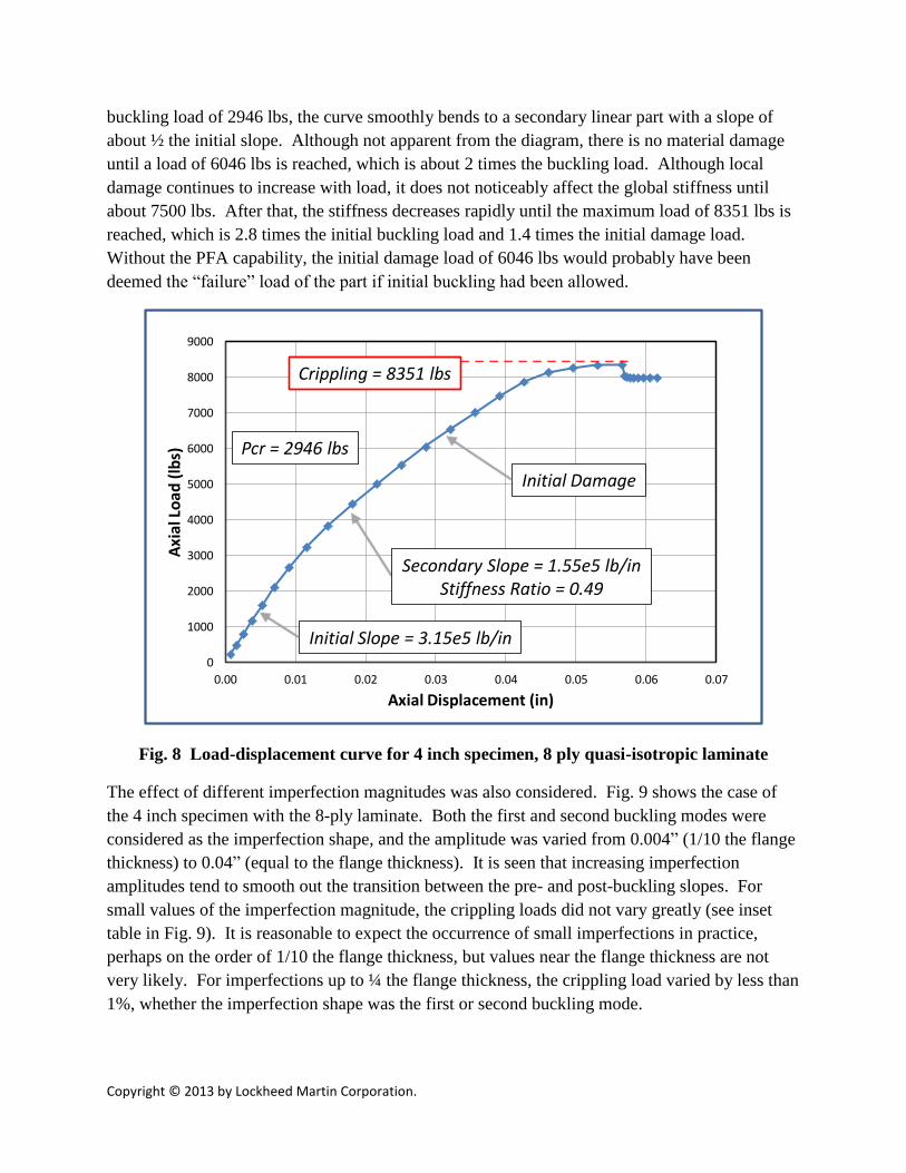
A load-displacement diagram was constructed for each nonlinear run. Fig. 8 shows the diagram

for the 4 inch specimen with the 8 ply quasi-isotropic laminate. The initial imperfection in this

case had the shape of the first buckling mode, with an amplitude of 0.01 inch (corresponding to

¼ the flange thickness). The curve shows the expected characteristics discussed in regards to

Fig. 2. The initial slope corresponds to the member axial stiffness given by AE/L. Near the

L = 4”Pcr = 2946 lbs

L = 8”Pcr = 2706 lbs

L = 6”Pcr = 2774 lbs

L = 12”Pcr = 2652 lbs


buckling load of 2946 lbs, the curve smoothly bends to a secondary linear part with a slope of

about ½ the initial slope. Although not apparent from the diagram, there is no material damage

until a load of 6046 lbs is reached, which is about 2 times the buckling load. Although local

damage continues to increase with load, it does not noticeably affect the global stiffness until

about 7500 lbs. After that, the stiffness decreases rapidly until the maximum load of 8351 lbs is

reached, which is 2.8 times the initial buckling load and 1.4 times the initial damage load.

Without the PFA capability, the initial damage load of 6046 lbs would probably have been

deemed the “failure” load of the part if initial buckling had been allowed.

Fig. 8 Load-displacement curve for 4 inch specimen, 8 ply quasi-isotropic laminate

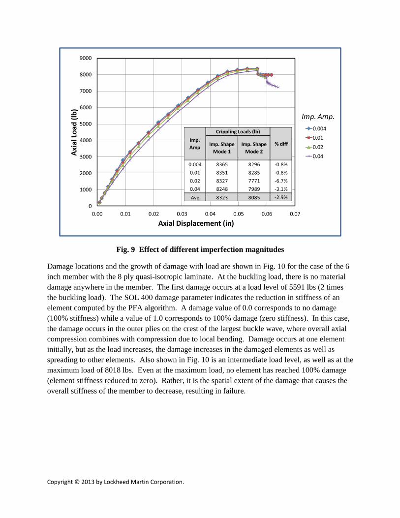
The effect of different imperfection magnitudes was also considered. Fig. 9 shows the case of

the 4 inch specimen with the 8-ply laminate. Both the first and second buckling modes were

considered as the imperfection shape, and the amplitude was varied from 0.004” (1/10 the flange

thickness) to 0.04” (equal to the flange thickness). It is seen that increasing imperfection

amplitudes tend to smooth out the transition between the pre- and post-buckling slopes. For

small values of the imperfection magnitude, the crippling loads did not vary greatly (see inset

table in Fig. 9). It is reasonable to expect the occurrence of small imperfections in practice,

perhaps on the order of 1/10 the flange thickness, but values near the flange thickness are not

very likely. For imperfections up to ¼ the flange thickness, the crippling load varied by less than

1%, whether the imperfection shape was the first or second buckling mode.

0

1000

2000

3000

4000

5000

6000

7000

8000

9000

0.00 0.01 0.02 0.03 0.04 0.05 0.06 0.07

Axi

al L

oa

d (

lbs)

Axial Displacement (in)

Initial Slope = 3.15e5 lb/in

Secondary Slope = 1.55e5 lb/inStiffness Ratio = 0.49

Crippling = 8351 lbs

Initial Damage

Pcr = 2946 lbs


Fig. 9 Effect of different imperfection magnitudes

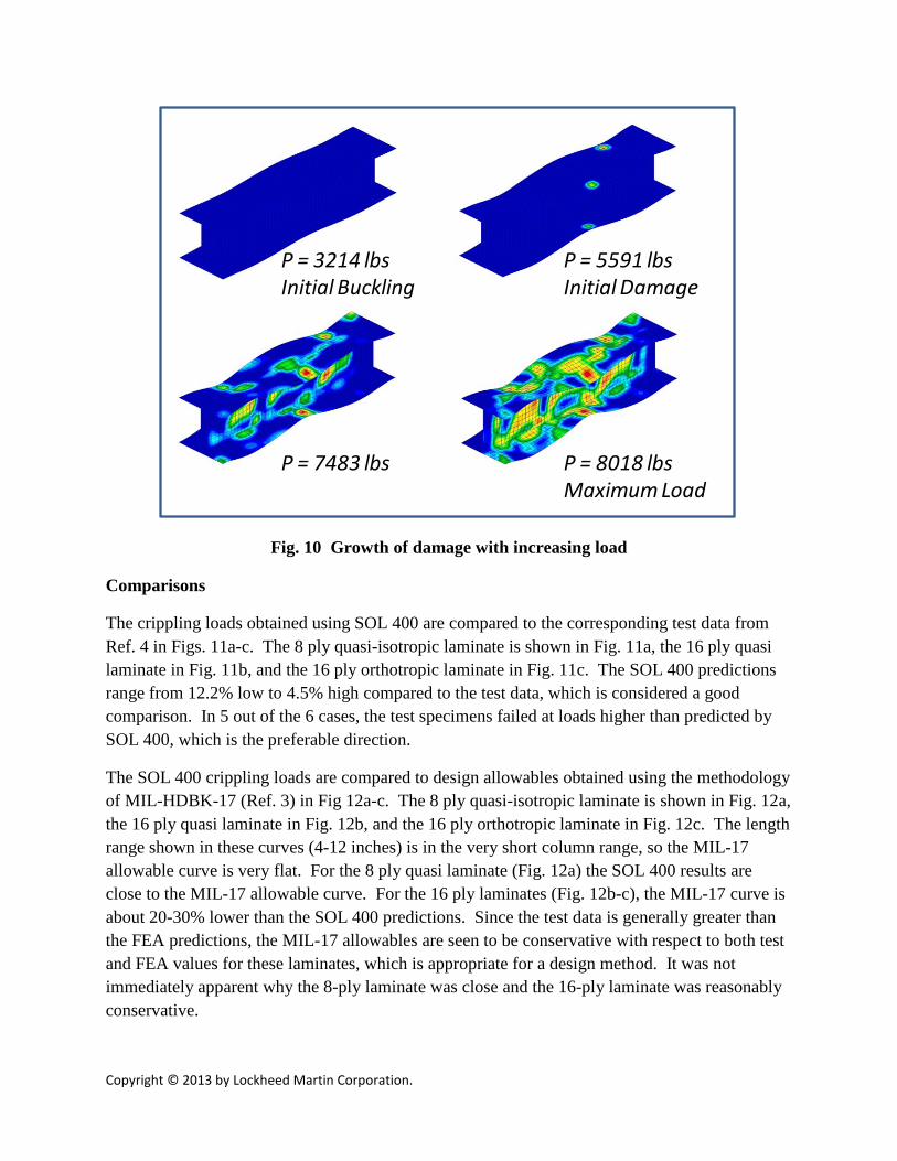
Damage locations and the growth of damage with load are shown in Fig. 10 for the case of the 6

inch member with the 8 ply quasi-isotropic laminate. At the buckling load, there is no material

damage anywhere in the member. The first damage occurs at a load level of 5591 lbs (2 times

the buckling load). The SOL 400 damage parameter indicates the reduction in stiffness of an

element computed by the PFA algorithm. A damage value of 0.0 corresponds to no damage

(100% stiffness) while a value of 1.0 corresponds to 100% damage (zero stiffness). In this case,

the damage occurs in the outer plies on the crest of the largest buckle wave, where overall axial

compression combines with compression due to local bending. Damage occurs at one element

initially, but as the load increases, the damage increases in the damaged elements as well as

spreading to other elements. Also shown in Fig. 10 is an intermediate load level, as well as at the

maximum load of 8018 lbs. Even at the maximum load, no element has reached 100% damage

(element stiffness reduced to zero). Rather, it is the spatial extent of the damage that causes the

overall stiffness of the member to decrease, resulting in failure.

0

1000

2000

3000

4000

5000

6000

7000

8000

9000

0.00 0.01 0.02 0.03 0.04 0.05 0.06 0.07

Axi

al L

oa

d (

lb)

Axial Displacement (in)

0.004

0.01

0.02

0.04

0.004 8365 8296 -0.8%

0.01 8351 8285 -0.8%

0.02 8327 7771 -6.7%

0.04 8248 7989 -3.1%

Avg 8323 8085 -2.9%

Imp.

Amp

Crippling Loads (lb)

% diffImp. Shape

Mode 1

Imp. Shape

Mode 2

Imp. Amp.


Fig. 10 Growth of damage with increasing load

Comparisons

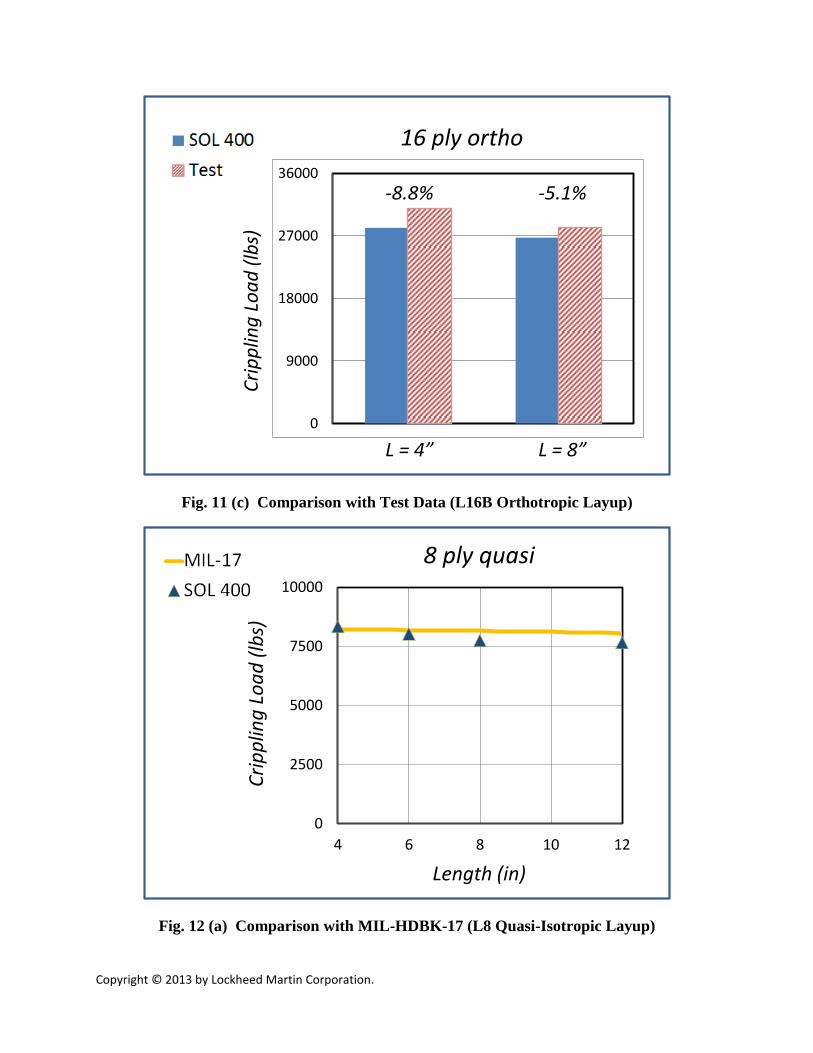
The crippling loads obtained using SOL 400 are compared to the corresponding test data from

Ref. 4 in Figs. 11a-c. The 8 ply quasi-isotropic laminate is shown in Fig. 11a, the 16 ply quasi

laminate in Fig. 11b, and the 16 ply orthotropic laminate in Fig. 11c. The SOL 400 predictions

range from 12.2% low to 4.5% high compared to the test data, which is considered a good

comparison. In 5 out of the 6 cases, the test specimens failed at loads higher than predicted by

SOL 400, which is the preferable direction.

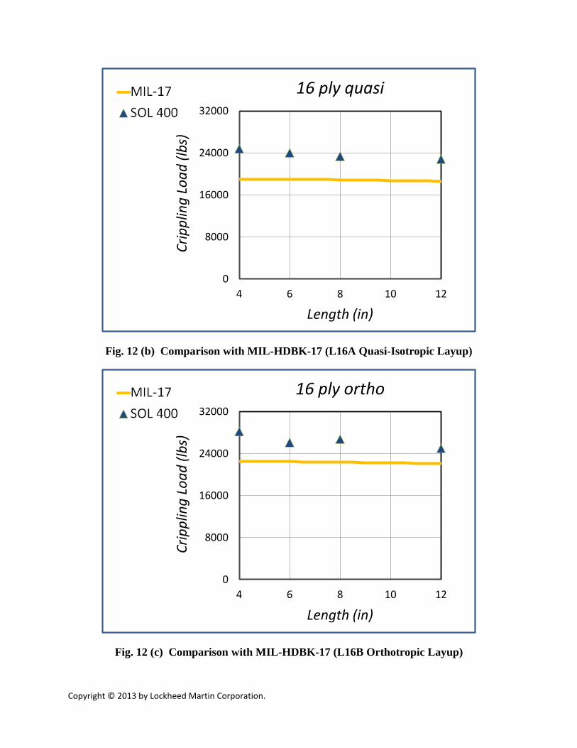
The SOL 400 crippling loads are compared to design allowables obtained using the methodology

of MIL-HDBK-17 (Ref. 3) in Fig 12a-c. The 8 ply quasi-isotropic laminate is shown in Fig. 12a,

the 16 ply quasi laminate in Fig. 12b, and the 16 ply orthotropic laminate in Fig. 12c. The length

range shown in these curves (4-12 inches) is in the very short column range, so the MIL-17

allowable curve is very flat. For the 8 ply quasi laminate (Fig. 12a) the SOL 400 results are

close to the MIL-17 allowable curve. For the 16 ply laminates (Fig. 12b-c), the MIL-17 curve is

about 20-30% lower than the SOL 400 predictions. Since the test data is generally greater than

the FEA predictions, the MIL-17 allowables are seen to be conservative with respect to both test

and FEA values for these laminates, which is appropriate for a design method. It was not

immediately apparent why the 8-ply laminate was close and the 16-ply laminate was reasonably

conservative.

P = 3214 lbsInitial Buckling

P = 7483 lbs

P = 5591 lbsInitial Damage

P = 8018 lbsMaximum Load


Fig. 11 (a) Comparison with Test Data (L8 Quasi-Isotropic Layup)

Fig. 11 (b) Comparison with Test Data (L16A Quasi-Isotropic Layup)

8 ply quasi

0

2500

5000

7500

10000

L = 4” L = 8”

+4.5% -6.1%

Cri

pp

ling

Lo

ad

(lb

s)

16 ply quasi

0

8000

16000

24000

32000

L = 4” L = 8”

-9.2% -12.2%

Cri

pp

ling

Lo

ad

(lb

s)


Fig. 11 (c) Comparison with Test Data (L16B Orthotropic Layup)

Fig. 12 (a) Comparison with MIL-HDBK-17 (L8 Quasi-Isotropic Layup)

16 ply ortho

0

9000

18000

27000

36000

L = 4” L = 8”

-8.8% -5.1%

Cri

pp

ling

Lo

ad

(lb

s)

0

2500

5000

7500

10000

4 6 8 10 12

8 ply quasi

Cri

pp

ling

Lo

ad

(lb

s)

Length (in)


Fig. 12 (b) Comparison with MIL-HDBK-17 (L16A Quasi-Isotropic Layup)

Fig. 12 (c) Comparison with MIL-HDBK-17 (L16B Orthotropic Layup)

0

8000

16000

24000

32000

4 6 8 10 12

16 ply quasi

Cri

pp

ling

Lo

ad

(lb

s)

Length (in)

0

8000

16000

24000

32000

4 6 8 10 12

16 ply ortho

Cri

pp

ling

Lo

ad

(lb

s)

Length (in)


Conclusions

The nonlinear load-displacement curves obtained using SOL 400 with PFA followed the

expected trends, and the predicted crippling loads agreed fairly well with available test data

(+4.5% to -12.2%). The initial buckling loads obtained using SOL 105 were significantly lower

than test (-22% to -49%). These differences may be due to deficiencies in the model or

difficulties in determining initial buckling from a test and although not pursued here are worth

further investigation.

The MIL-HDBK-17 derived crippling allowables are close to FEA predictions for the 8-ply

laminates, but are about 20-30% low for the 16-ply laminates. As a design methodology, rather

than a prediction tool, it is appropriate that the MIL-17 values are conservative with respect to

both test and FEA, but it was not discovered why there was a difference between the 8-ply and

16-ply laminates in this regard.

Here, we only used buckling and crippling loads from Ref. 4 for comparison, which also used an

older material type. For more complete verification, additional specimens should be built and

tested using fully characterized current materials, and complete data collected during the tests,

including number of buckling waves, load-displacement curves, strain distributions, and failure

modes. This would allow more detailed comparisons to be made with the FEA results, help

identify and explain discrepancies, and would increase confidence in the methodology.

The PFA capability of MSC Nastran SOL 400 is a promising tool to predict final failure, rather

than just initial failures, of laminated composite structures. It was shown in this paper that in

certain cases, final global failure can occur at loads well above initial local failure (e.g. 8351 vs.

6046 lbs, Fig. 8). Therefore, SOL 400 PFA offers the potential to more fully utilize the

capabilities of composite materials.

Acknowledgements

Thanks to William Zivich, IRAD Principal Investigator for funding this study, John Scarcello

(Manager) and Eric Horton (Senior Manager) for supporting attendance at the 2013 MSC Users

Conference, and Hanson Chang and James Filon of MSC for providing sample input files and

assistance in performing the analyses.

References

1. Bulson, P.S., The Stability of Flat Plates, Elsevier, 1969

2. Gerard, G., Handbook of Structural Stability, Part IV, Failure of Plates and Composite

Elements, Technical Note 3784, National Advisory Committee for Aeronautics, 1957

3. Composite Materials Handbook, MIL-HDBK-17F, Volume 3, Polymer Matrix

Composite Materials Usage Design and Analysis, Department of Defense, 2002


4. Bonanni, D.L., Johnson, E.R., Starnes, J.H., “Local Crippling of Thin-Walled Graphite-

Epoxy Stiffeners”, AIAA paper 88-2251, 1988

5. MSC Nastran 2012.2 Quick Reference Guide, Rev 0, June 26, 2012

6. Singer, J., Arbocz, J., Weller, T., Buckling Experiments: Experimental Methods in

Buckling of Thin-Walled Structures, John Wiley & Sons, 1998

crippling of thin-walled composite sections using...

Documents