credit valuation adjustment - kth · this thesis is intended to give an overview of credit...
TRANSCRIPT

KTH - Royal Institute of Technology
Master’s Thesis
Credit Valuation AdjustmentIn theory and practice
Author:
Dan Franzen
Otto Sjoholm
Supervisor:
Dr. Henrik Hult
A thesis submitted in fulfilment of the requirements
for the degree of Master in Financial Mathematics
at the
Division of Mathematical Statistics
Department of Mathematics
January 2014

KTH - ROYAL INSTITUTE OF TECHNOLOGY
Abstract
Department of Mathematics
Master in Financial Mathematics
Credit Valuation Adjustment
by
Dan Franzen & Otto Sjoholm
This thesis is intended to give an overview of credit valuation adjustment (CVA) and ad-
jacent concepts. Firstly, the historical events that preceded the initiative to reform the
Basel regulations and to introduce CVA as a core component of counterparty credit risk
are illustrated. After some conceptual background material, a journey is taken through
the regulatory aspects of CVA. The three most commonly used methods for calculating
the regulatory CVA capital charge are explained in detail and potential challenges with
the methods are addressed. Further, the document analyses in greater depth two of the
methods; the internal model method (IMM) and the current exposure method (CEM).
The differences between these two methods are explained mathematically and analysed.
This comparison is supported by simulations of portfolios containing interest rate swap
contracts with different time to maturity and of counterparties with varying credit rat-
ings. One concluding observations is that credit valuation adjustment is a measure of
central importance within counterparty credit risk. Further, it is shown that IMM has
some important advantages over CEM, especially when it comes to model connection
with reality. Finally, some possible future work to be done within the topic area is
suggested.
Keywords: Basel II, Basel III, OTC Derivatives, Credit Valuation Adjustment, CVA,
Counterparty Credit Risk, CCR, Internal Model Method, Current Exposure Method, Reg-
ulations, Interest Rate Swap, DVA, LVA, FVA, OCA

Acknowledgements
We would like to extend our great thanks and appreciation to Dr. Henrik Hult at the
Department of Financial Mathematics at the Royal Institute of Technology (KTH) for
his engaged supervision. Dr. Hult has with his expertise been given us invaluable guid-
ance through challenging moments during this thesis. We would also like to thank Ola
Hammarlid at Swedbank, LCI for engagement and inputs regarding our topic, credit
valuation adjustment. We would also like to thank our families for support and proof-
reading of the thesis.
ii
Contents
Abstract i
Acknowledgements ii
List of Figures vi
List of Tables viii
Abbreviations ix
1 Introduction 1
1.1 Thesis demarcation . . . . . . . . . . . . . . . . . . . . . . . . . . . . . . . 1
1.2 Historical background . . . . . . . . . . . . . . . . . . . . . . . . . . . . . 2
1.2.1 CCR - Counterparty credit risk . . . . . . . . . . . . . . . . . . . . 2
1.2.2 The financial crisis and the too-big-to-fail concept . . . . . . . . . 3
1.2.3 The emergence of CVA . . . . . . . . . . . . . . . . . . . . . . . . 4
2 Conceptual Background 7
2.1 CVA - Credit valuation adjustment . . . . . . . . . . . . . . . . . . . . . . 7
2.1.1 Different contexts . . . . . . . . . . . . . . . . . . . . . . . . . . . . 7
2.1.2 Definition . . . . . . . . . . . . . . . . . . . . . . . . . . . . . . . . 9
2.2 OTC derivatives . . . . . . . . . . . . . . . . . . . . . . . . . . . . . . . . 10
2.3 Netting and ISDA Master Agreements . . . . . . . . . . . . . . . . . . . . 11
2.4 Collateral and CSA . . . . . . . . . . . . . . . . . . . . . . . . . . . . . . . 14
2.5 Central counterparty clearing . . . . . . . . . . . . . . . . . . . . . . . . . 15
2.6 Wrong way risk . . . . . . . . . . . . . . . . . . . . . . . . . . . . . . . . . 17
2.7 CVA optimization . . . . . . . . . . . . . . . . . . . . . . . . . . . . . . . 18
2.8 Bilateral CVA . . . . . . . . . . . . . . . . . . . . . . . . . . . . . . . . . . 19
2.9 XVAs - Additional valuation adjustments . . . . . . . . . . . . . . . . . . 20
2.9.1 DVA - Debit valuation adjustment . . . . . . . . . . . . . . . . . . 20
2.9.2 LVA - Liquidity valuation adjustment . . . . . . . . . . . . . . . . 22
2.9.3 FVA - Funding valuation adjustment . . . . . . . . . . . . . . . . . 22
2.9.4 OCA - Own credit adjustment . . . . . . . . . . . . . . . . . . . . 22
3 Mathematical Definitions 24
3.1 PV - Present value . . . . . . . . . . . . . . . . . . . . . . . . . . . . . . . 24
3.2 Exposure . . . . . . . . . . . . . . . . . . . . . . . . . . . . . . . . . . . . 25
iii

Contents iv
3.3 PD - Probability of Default . . . . . . . . . . . . . . . . . . . . . . . . . . 25
3.4 LGD - Loss Given Default . . . . . . . . . . . . . . . . . . . . . . . . . . . 26
3.5 EAD - Exposure at Default . . . . . . . . . . . . . . . . . . . . . . . . . . 27
4 Regulations 28
4.1 Basel II . . . . . . . . . . . . . . . . . . . . . . . . . . . . . . . . . . . . . 28
4.2 Basel III . . . . . . . . . . . . . . . . . . . . . . . . . . . . . . . . . . . . . 29
4.3 CRD IV and CRR . . . . . . . . . . . . . . . . . . . . . . . . . . . . . . . 30
4.3.1 LCR - Liquidity Coverage Ratio and NSFR - Net Stable FundingRequirement . . . . . . . . . . . . . . . . . . . . . . . . . . . . . . 31
4.3.2 HQLA - High Quality Liquid Asset . . . . . . . . . . . . . . . . . . 32
4.4 Regulations of OTC instruments . . . . . . . . . . . . . . . . . . . . . . . 33
5 Regulatory Methods 34
5.1 Introduction to Regulatory Methods . . . . . . . . . . . . . . . . . . . . . 34
5.1.1 Regulatory separation of risks . . . . . . . . . . . . . . . . . . . . . 34
5.1.2 RWA - Risk-weighted assets . . . . . . . . . . . . . . . . . . . . . . 35
5.1.3 Regulatory approaches to credit risk . . . . . . . . . . . . . . . . . 35
5.1.4 Regulatory CVA methods . . . . . . . . . . . . . . . . . . . . . . . 36
5.2 Standardized Approach . . . . . . . . . . . . . . . . . . . . . . . . . . . . 38
5.2.1 SM - Standardized Method . . . . . . . . . . . . . . . . . . . . . . 40
5.2.2 CEM - Current Exposure Method . . . . . . . . . . . . . . . . . . 41
5.2.3 A note on future non-internal model methods . . . . . . . . . . . . 44
5.2.4 IMM - Internal Model Method . . . . . . . . . . . . . . . . . . . . 45
5.3 Advanced Approach . . . . . . . . . . . . . . . . . . . . . . . . . . . . . . 49
5.3.1 AM - Advanced Method . . . . . . . . . . . . . . . . . . . . . . . . 49
6 CVA calculation for interest rate swaps 53
6.1 Calculation methods . . . . . . . . . . . . . . . . . . . . . . . . . . . . . . 53
6.2 The interest rate swap . . . . . . . . . . . . . . . . . . . . . . . . . . . . . 54
6.3 The discount curve . . . . . . . . . . . . . . . . . . . . . . . . . . . . . . . 56
6.4 Internal Model Method (IMM) . . . . . . . . . . . . . . . . . . . . . . . . 57
6.4.1 Interest rate simulations . . . . . . . . . . . . . . . . . . . . . . . . 59
6.4.2 Exposures . . . . . . . . . . . . . . . . . . . . . . . . . . . . . . . . 61
6.5 Current Exposure Method (CEM) . . . . . . . . . . . . . . . . . . . . . . 63
7 Results and Conclusion 64
7.1 Stress Tests . . . . . . . . . . . . . . . . . . . . . . . . . . . . . . . . . . . 64
7.1.1 Stress test 1 - Rating drop . . . . . . . . . . . . . . . . . . . . . . . 64
7.1.2 Stress test 2 - Increasing time to maturity, fixed rating AA . . . . 66
7.1.3 Stress test 3 - Increasing time to maturity, fixed rating BBB . . . 68
7.1.4 Stress test 4 - Manipulation of Credit Conversion Factor . . . . . . 69
7.1.5 Comparison of credit rating and maturity stress . . . . . . . . . . 70
7.1.6 Netting and NGR complications . . . . . . . . . . . . . . . . . . . 71
7.2 Last words about CEM & IMM . . . . . . . . . . . . . . . . . . . . . . . . 74
7.2.1 CVA calculation computer intensiveness . . . . . . . . . . . . . . . 74
7.2.2 Other aspects of CEM & IMM . . . . . . . . . . . . . . . . . . . . 74
7.2.3 Challenges in obtaining IMM approval . . . . . . . . . . . . . . . . 75

Contents v
7.3 Conclusion . . . . . . . . . . . . . . . . . . . . . . . . . . . . . . . . . . . 76
7.4 Future work within the topic area . . . . . . . . . . . . . . . . . . . . . . . 76
A Matlab Code 78
A.1 main.m . . . . . . . . . . . . . . . . . . . . . . . . . . . . . . . . . . . . . . 78
A.2 func read rating data.m . . . . . . . . . . . . . . . . . . . . . . . . . . . 81
A.3 func create rate spec.m . . . . . . . . . . . . . . . . . . . . . . . . . . . 82
A.4 func read swap data.m . . . . . . . . . . . . . . . . . . . . . . . . . . . . 83
A.5 func imm epe.m . . . . . . . . . . . . . . . . . . . . . . . . . . . . . . . . . 85
A.6 func imm eff maturity.m . . . . . . . . . . . . . . . . . . . . . . . . . . . 91
A.7 func cem ead.m . . . . . . . . . . . . . . . . . . . . . . . . . . . . . . . . . 92
A.8 func cem eff maturity.m . . . . . . . . . . . . . . . . . . . . . . . . . . . 94
A.9 func hw level.m . . . . . . . . . . . . . . . . . . . . . . . . . . . . . . . . 96
Bibliography 97

List of Figures
1.1 Counterparty credit risk lies in the area of risk where market and creditrisks intersect. This makes an accurate risk assessment complicated. . . . 2
1.2 Total global trade in OTC derivatives 1998-2013, showing the aggregatenotional amounts of the different derivative types. . . . . . . . . . . . . . 5
2.1 Fictitious probability distribution of credit exposure, indicating whereaccounting CVA and regulatory CVA are located. . . . . . . . . . . . . . . 9
2.2 Example of netting 2 separate contracts . . . . . . . . . . . . . . . . . . . 12
2.3 Collateral is transferred from B to A if the mark-to-market value of theOTC derivative reaches a certain limit. . . . . . . . . . . . . . . . . . . . . 14
2.4 Generally, the CVA may be mitigated by moving to collateralizationmethods more to the right in this graph. The best method being touse a CCP [10]. . . . . . . . . . . . . . . . . . . . . . . . . . . . . . . . . . 16
2.5 The amount of transferred capital between counterparties may be sub-stantially reduced by using netting a agreements, and even further byusing central counterparty clearing. . . . . . . . . . . . . . . . . . . . . . . 17
2.6 Wrong way risk arises when a high exposure is correlated with a low creditrating towards a counterparty. . . . . . . . . . . . . . . . . . . . . . . . . . 17
5.1 The two approaches and four different methods for calculating the CVAcapital requirement. . . . . . . . . . . . . . . . . . . . . . . . . . . . . . . 37
5.2 The 10-day CVA VaR with 90% confidence. The figure was extractedfrom Jon Gregory’s presentation [21]. . . . . . . . . . . . . . . . . . . . . . 50
6.1 An interest rate swap agreement between bank A and B with the floatingleg tied to the EURIBOR rate. . . . . . . . . . . . . . . . . . . . . . . . . 55
6.2 If the MtM value is positive when your counterparty defaults, you willlose a value of LGD ×MtM . . . . . . . . . . . . . . . . . . . . . . . . . . 56
6.3 The initial yield curve at settlement date built from the rates in the abovetable. . . . . . . . . . . . . . . . . . . . . . . . . . . . . . . . . . . . . . . 57
6.4 The EURIBOR rate in 2013 is much lower than it has been historically.The dotted line represents the 3M rate data, which is used for the shortrate simulations. . . . . . . . . . . . . . . . . . . . . . . . . . . . . . . . . 59
6.5 The simulated yield curve evolution of scenario 15. The short rate keepslow during the five year period. . . . . . . . . . . . . . . . . . . . . . . . . 61
6.6 The simulated yield curve evolution of scenario 16. The short rate in-creases noticeably during the five year period. . . . . . . . . . . . . . . . . 61
6.7 The MtM price evolution of a small portfolio of 5-year interest rate swaps. 62
vi

List of Figures vii
7.1 CVA simulated for 4 different contracts with declining credit rating butfixed time-to-maturity . . . . . . . . . . . . . . . . . . . . . . . . . . . . . 65
7.2 CVA simulated for 5 contracts with same credit rating AA and increasingtime-to-maturity, using the CEM and IMM. . . . . . . . . . . . . . . . . . 67
7.3 CVA simulated for 5 contracts with same credit rating BBB and increasingtime-to-maturity, using CEM and IMM method . . . . . . . . . . . . . . 68
7.4 CVA capital charge computed using IMM and CEM for BBB-rated coun-terparty, with manipulated credit conversion factor. . . . . . . . . . . . . 70
7.5 CVA capital charge computed using IMM and CEM. . . . . . . . . . . . . 71
7.6 CVA capital charge computed using IMM and two different values of NGRunder CEM, for an AA-rated counterparty. . . . . . . . . . . . . . . . . . 73

List of Tables
5.1 Correspondence between counterparty rating and CVA weight accordingto Basel III. . . . . . . . . . . . . . . . . . . . . . . . . . . . . . . . . . . . 39
5.2 Credit conversion factors (CCFs) for different contract types and matu-rities. All factors are given in percent (%). . . . . . . . . . . . . . . . . . . 42
6.1 Initial rates used in the CVA calculation. . . . . . . . . . . . . . . . . . . 57
7.1 CVA computed for 4 different counterparties with different rating but thesame time-to-maturity, using CEM and IMM method . . . . . . . . . . . 65
7.2 CVA simulated for 5 contracts with same credit rating AA and increasingtime-to-maturity, using the CEM and IMM. . . . . . . . . . . . . . . . . . 66
7.3 Fraction of CVA CV AIMMCV ACEM
for AA rated contract and 1-5 years to maturity. 67
7.4 CVA simulated for 5 contracts with same credit rating BBB and increasingtime-to-maturity, using CEM and IMM method. . . . . . . . . . . . . . . 68
7.5 Fraction of CVA value CV AIMMCV ACEM
for BBB rated contract and 1-5 years tomaturity. . . . . . . . . . . . . . . . . . . . . . . . . . . . . . . . . . . . . 68
7.6 Credit conversion factor for CEM in the standard embodiment . . . . . . 69
7.7 Credit conversion factor for CEM in the stressed scenario with fixed creditconversion factor . . . . . . . . . . . . . . . . . . . . . . . . . . . . . . . . 69
viii

Abbreviations
A-IRB Advanced Internal Rating Based Approach
ATM At The Money
BCBS Basel Committee on Banking Supervision
CCDS Contingent Credit Default Swap
CCF Credit Conversion Factor
CCP Central CounterParty
CCR Counterparty Credit Risk
CDF Cumulative Distribution Function
CDS Credit Default Swap
CE Current Exposure
CEM Current Exposure Method
CET Core Equity Tier
CM Clearing Member
CRD Capital Requirements Directive
CRR Capital Requirements Regulations
CSA Credit Support Annex
CVA Credit Valuation Adjustment
DF Discount Factor
DVA Debit Valuation Adjustment
EAD Exposure At Default
EEE Effective Expected Exposure
EEPE Effective Expected Positive Exposure
F-IRB Funding Internal Rating Based Approach
FVA Funding Value Adjustment
HQLA High Quality Liquid Asset
ix

Abbreviations x
IFRS International Financial Reporting Standards
IMM Internal Model Method
IRS Interest Rate Swap
ICAAP International Capital Adequacy Assessment Process
ISDA International Swaps Derivatives Association
ITM In The Money
LCR Liquidity Coverage Ratio
LGD Loss Given Default
LVA Liquidity Value Adjustment
LTCM Long Term Capital Management
MTM Mark To Market
NGR Net-to Gross Ratio
NIMM Non Internal Model Method
NSFR Net Stable Funding Requirement
OCA Own Credit Adjustment
OCI Other Comprehensive Iincome
OTC Over The Counter
OTF Organized Trading Facility
PD Probability of Default
PV Present Value
PFE Potential Future Exposure
RC Replacement Cost
Repo Repurchase Agreement
RWA Risk Weighted Asset
SFT Structured Finance Transaction
SM Standard Method
VaR Value at Risk
WWR Wrong Way Risk

Chapter 1
Introduction
1.1 Thesis demarcation
This thesis is intended to give a comprehensive description of the concept credit valuation
adjustment - CVA. We will go through its origin, the different usages of this adjustment,
and describe a few ways to model CVA on a daily basis. In order to try and convey an
as complete and clear picture as possible, concepts of surrounding domains will also be
included to some extent.
The purpose of the demarcation of the thesis is firstly explaining the key concepts of
CVA in a comprehendable manner. Secondly, concentrating more on the very core of
the regulation aspect of CVA, by performing simulations and analysis of how CVA is
affected by the most basic and closely related variables. Hence, the more complex factors
and concepts related to CVA; such as collateral, central counterparties and wrong way
risks, are carefully explained, but not analysed in any greater depth in this thesis.
Our hope is that the reader of this document will gain a broad understanding of the
origin and need for the CVA within the financial sector. The reader should be able
to perceive the complexities involved in assessing CVA, but at the same time get a
feeling of how these complexities may be managed properly. Moreover, we hope that the
simulations and analysis presented may give a hint of how to calculate CVA for some
simple financial instruments and portfolios.
1

Chapter 1. Introduction 2
1.2 Historical background
In this section, a brief historical background to CVA will be given. It contains a brief
description of the developments of counterparty credit risk (CCR) since the financial
crisis of 2007-2008, as well as the emergence of the rather new concept of credit valuation
adjustment.
1.2.1 CCR - Counterparty credit risk
Some of the greatest advancements in the financial industry have taken place in times
of financial distress or crisis. Systems or models that are thought to be valid, are often
foiled and proven not to reflect reality in such times. Just like other reversals in the
industry, both the collapse of Long Term Capital Management (LTCM) and the financial
crisis of 2007-2008 have triggered progress in the sector. One of the most significant
advances is that many financial institutions have been driven to review and change their
measurement and assessment of both market and credit risk, but especially counterparty
credit risk. In order to understand the historical development of counterparty credit risk,
we will start by explaining these three different types of risk and how they relate to each
other.
Firstly, market risk (sometimes systematic risk) is the risk of losses due to movements
in market prices. It is focused on factors that affect the financial market as a whole
and not specific prices. Secondly, credit risk is the risk of financial losses arising from a
borrower’s failure to meet a contractual obligation. This risk type usually covers classic
instruments like mortgage loans and bonds.
Figure 1.1: Counterparty credit risk lies in the area of risk where market and creditrisks intersect. This makes an accurate risk assessment complicated.

Chapter 1. Introduction 3
Counterparty credit risk is closely related to, but strictly not a type of credit risk, as
the name would suggest. CCR is defined as the risk that a counterparty defaults before
honoring its engagements. Hence, its definition is very similar to that of credit risk.
But, unlike credit risk, CCR covers loans and repurchase agreement (Repo) transactions
and, most importantly, over-the-counter (OTC) derivatives. The special thing about
CCR is that it inherits both market and credit risks. Therefore, dealing with CCR is
no easy task, since it requires knowledge in both credit risk and market risk, as well as
understanding the synergies between the two. The reason for this will be explained in
detail in Section 2.1.
1.2.2 The financial crisis and the too-big-to-fail concept
The notion of default and its consequences have long been understood by investors.
Despite this, the risk associated with counterparty defaults were by most institutions
not properly incorporated into their risk system before the crisis. Due to this, CCR has
gained a lot of attention lately.
Before the LTCM collapsed, most firms involved in the financial market used credit
measures and limits to control their possible exposure to a counterparty in the future.
The liquidation of LTCM definitely increased the interest in CCR, although mostly by
the largest banks. A few years later, starting in 2004, accounting standards were set
up (FASB 157 and IAS 39) regarding counterparty risk. The purpose of the standards
were that the value of a derivatives position must be corrected for its counterparty risk.
As a consequence all banks had to start calculating a measure called credit valuation
adjustment (CVA) on a monthly basis [5].
At this time there still existed a wide spread belief in a concept called too-big-to-fail.
The concept implies that a institution is so huge that its default would have disastrous
consequences on the economy. Therefore, in case of distress, the government would go
in and support the institution in order to prevent it to default. A large portion of the
institutions in the sector were considered to be precisely too-big-to-fail even until the
financial crisis was a fact.
The IBM Business Analytics department summarizes briefly the history of the deriva-
tives market in the following way. ”In the early days of the derivatives markets, there

Chapter 1. Introduction 4
was a tendency to deal only with the most credit-worthy institutions. Less worthy
counterparties were either excluded entirely, or were presented with additional trading
requirements, such as paying substantial premiums or agreeing to tight collateral terms.
The result was that financial institutions set up triple-A rated bankruptcy-remote sub-
sidiaries to handle their derivatives operations, and monoline insurers took massive one-
way risks based on the flawed notion that their triple-A credit quality immunized those
trading with them against CCR, even in the absence of commonly used collateral agree-
ments. The credit crisis has brought CCR to prominence now that the attitude of ’too
big to fail’ is dispelled and CCR is now considered by many to be the key financial risk.”
[4]
Once the crisis hit and Lehman Brothers went into bankruptcy, the too-big-to-fail belief
was unpleasantly proven not to be applicable at all times. If the fourth largest investment
bank in the United States is allowed to go into bankruptcy, then no other institution
could certainly be too-big-to-fail.
1.2.3 The emergence of CVA
Historically, the rate at which borrowing and lending were carried out between many
large financial institutions was set equal to the risk free rate. This since the counter-
parties often were considered to be of the type to-big-to-fail. Vladimir Piterbarg notes
in his article that this is not an adequate approach. ”Standard derivatives pricing the-
ory (see, for example, Hull, 2006) relies on the assumption that one can borrow and
lend at a unique risk-free rate. The realities of being a derivatives desk are, however,
rather different these days, as historically stable relationships between bank funding
rates, government rates, Libor rates, etc, have broken down.” [1, p.97]
What the derivatives market needed was a new risk measure to enable fair pricing when
including CCR. Hence, the new measure CVA was introduced in order to adjust for the
risk that appears for counterparties of derivative instruments. CVA is the difference
between the risk free value of a portfolio and the true value of that portfolio, accounting
for the possible default of a counterparty. Below one advantage of CVA is described
by the IBM Business Analytics department. ”Credit Value Adjustment (CVA) offers
an opportunity for banks to move beyond the control mindset of limits by dynamically
pricing counterparty credit risk directly into new trades. Many banks already measure

Chapter 1. Introduction 5
CVA in their accounting statements, but the financial crisis has led pioneering banks
to invest in systems that more accurately assess CVA, and integrate CVA into pre-deal
pricing and structuring.” [4]
Since CVA was first introduced, it has gained a more and more central role for par-
ticipants in the financial market, and especially the derivatives market. The frequency
at which CVA is calculated has increased massively at most firms. From being a risk
measure calculated once a month, many institutions now calculate CVA on a daily basis
or even in real-time.
One natural reason for the rising importance of CVA is the substantial growth of the
OTC derivatives market the last decade. As explained above, OTC derivatives today
make up a major portion of the CCR.
Figure 1.2: Total global trade in OTC derivatives 1998-2013, showing the aggregatenotional amounts of the different derivative types.
Figure 1.2 shows the value of the global trade in over-the-counter derivatives from 1998
to 2013. The reason to why OTC derivatives have an impact on the CCR will be
discussed in section 2.2.
The figure shows clearly that interest rate derivatives constitute the absolute body of
the value in the OTC derivatives market. Note that the values are not aggregated in
the figure, in the sense that the curves are stacked on top of each other.
As we have seen in this chapter, the financial market has lately been in great need of
a better way to assess the CCR. In order to improve the models, CVA was introduced

Chapter 1. Introduction 6
to capture a specific type of risk that had not been measured previously. In the next
chapter, CVA and a few other concept will be defined. These are necessary to fully
understand the complications involved in assessing CCR.

Chapter 2
Conceptual Background
2.1 CVA - Credit valuation adjustment
2.1.1 Different contexts
Some people may have difficulty in understanding the concept of CVA for one rather
inappropriate reason; the reason being that that there exist distinct definitions of the
adjustment in different financial domains. Hence, defining the CVA concept so that it
makes sense in all different aspects is a hard task, and it may lead to confusion using
definitions that are clearly contradicting each other. In order to somewhat remedy this
confusion we will already now point out two approaches towards the concept of CVA in
1. regulation,
2. accounting and pricing.
These two different aspects have distinct definitions and treatment of CVA. In the do-
main of regulation, CVA is measure of how much capital is needed to cover for losses due
to volatilities in counterparty credit spreads. Naturally, it is not enough only to have
capital covering the expected amount of losses. The capital amount should be enough to
cover the losses with a high probability. Hence, regulatory CVA is a VaR measure with a
certain large probability (currently 99%), that the regulatory capital covers future losses
due to the credit spread volatility of counterparties. This value is (in principle) always
7

Chapter 2. Conceptual Background 8
positive. This document almost exclusively consider the regulatory and VaR area of
CVA, but a brief background on accounting CVA is given for the sake of completeness.
In the context of accounting and pricing on the other hand, CVA is a measure to adjust
the risk-free value of an instrument to incorporate counterparty credit risk. From here
and on we refer to this type of CVA only as accounting CVA. Unlike regulatory CVA,
accounting CVA can be both positive or negative. The reason for this is that accounting
CVA is bilateral, a concept which will be fully described in section 2.8. Accounting
CVA is also closely related to a measure called DVA, which will be further discussed in
Section 2.9.1. The sign of the CVA depends on which of the two counterparties is most
likely to default and how the MTM value affects the owing between the counterparties.
Hence, CVA is here an expected value incorporating exposure and probability of default,
in order to achieve fair pricing.
One legitimate question is how these two CVA concepts are related. One natural way is
to look at the regulatory CVA as the potential future change (under a certain confidence
level) in the accounting CVA. Another fair question would be how the CVA capital charge
actually relates to credit spread volatility. Why is it that a CVA capital charge is needed
at all? Let us describe this by a process in a few steps.
1. There exists a volatility in the credit rating of a counterparty.
2. The volatility causes an uncertainty in the future expected value of accounting
CVA.
3. An uncertainty in the expected value of the accounting CVA also means a proba-
bility of MTM losses.
4. Regulatory CVA is held to cover the losses originating from the future loss prob-
ability distribution.
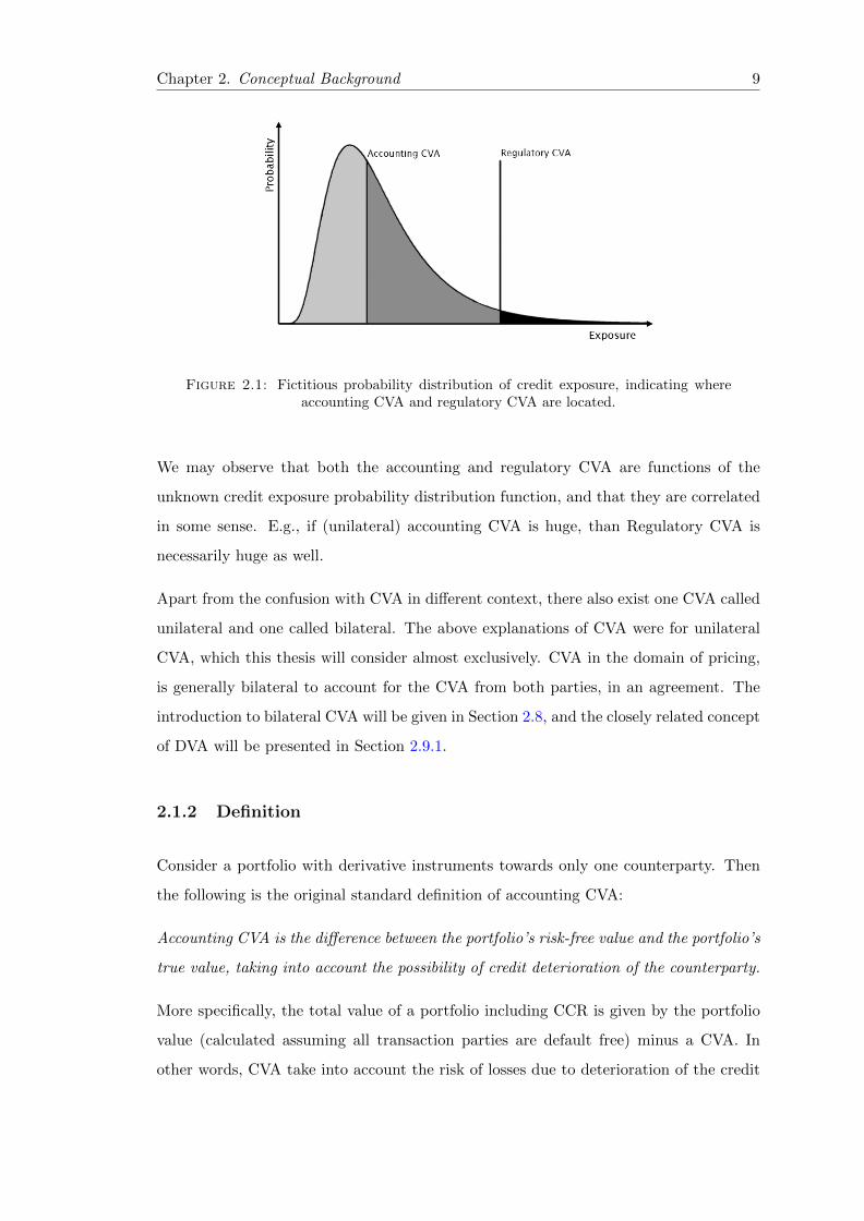
To get a feeling of the relation and difference of the two aspects of CVA, we may
benefit from observing Figure 2.1. In this figure, the curve shows a fictitious probability
distribution of the exposure, at a certain future time. In this distribution, the accounting
CVA is located at the expected value of the exposure. The regulatory CVA, on the
other hand, is found at the right quantile of the distribution and depends on both the
distribution itself and the confidence level used.
Chapter 2. Conceptual Background 9
Figure 2.1: Fictitious probability distribution of credit exposure, indicating whereaccounting CVA and regulatory CVA are located.
We may observe that both the accounting and regulatory CVA are functions of the
unknown credit exposure probability distribution function, and that they are correlated
in some sense. E.g., if (unilateral) accounting CVA is huge, than Regulatory CVA is
necessarily huge as well.
Apart from the confusion with CVA in different context, there also exist one CVA called
unilateral and one called bilateral. The above explanations of CVA were for unilateral
CVA, which this thesis will consider almost exclusively. CVA in the domain of pricing,
is generally bilateral to account for the CVA from both parties, in an agreement. The
introduction to bilateral CVA will be given in Section 2.8, and the closely related concept
of DVA will be presented in Section 2.9.1.
2.1.2 Definition
Consider a portfolio with derivative instruments towards only one counterparty. Then
the following is the original standard definition of accounting CVA:
Accounting CVA is the difference between the portfolio’s risk-free value and the portfolio’s
true value, taking into account the possibility of credit deterioration of the counterparty.
More specifically, the total value of a portfolio including CCR is given by the portfolio
value (calculated assuming all transaction parties are default free) minus a CVA. In
other words, CVA take into account the risk of losses due to deterioration of the credit

Chapter 2. Conceptual Background 10
quality of counterparties that do not default. Another popular and descriptive way to
define accounting CVA is the following:
Accounting CVA is the market value of the cost of credit spread’s volatility.
Moving over from accounting to regulatory CVA. The amount of capital needed to cover
the potential losses due to credit spread volatility is called the CVA capital charge. The
charge recognizes shifts in the credit spreads of the counterparty and ignores changes in
the market risk factors. The following would be a verbal definition of regulatory CVA:
Regulatory CVA is the amount of capital needed to cover for potential losses due to the
volatility in counterparty credit spreads.
As a motivation to why one would need a risk measure to capture shifts in credit spread,
the Basel Committee estimate that about three fourths of the CCR losses during the
financial crisis originate from CVA losses and not actual defaults. This is a remarkably
large fraction and it further bespeaks the obvious flaws that existed in risk systems
before the introduction of CVA.
Hopefully this section has given a brief but clear introduction the different aspects of
CVA and how they relate to each other. The purpose of the following sections is to
convey a more complete picture of CVA, by introducing a few closely related concepts.
2.2 OTC derivatives
As pointed out in section 1.2.1, the major part of a firm’s CCR is nowadays usually
built up by OTC derivatives. The complex structure of these derivatives make a reliable
computation of CCR much more difficult to perform than with most other risk types.
Firstly, calculating the relevant exposure is a difficult task. This is mainly because the
instrument future value is a function of the unknown future value(s) of the underlying
asset(s). Such future values can never be computed with a 100% accuracy. The unknown
future value however, is not something that is specific for derivative instruments, but is
rather a rule than exception for most financial instruments.
Secondly, an OTC derivative contract can either be an asset or a liability, depending
on the sign of its value. Thus, both parties of such a contract will face a counterparty
Chapter 2. Conceptual Background 11
credit risk during the lifetime of the contract. This is called being bilateral and will be
discussed in more detail in the section 2.9.1.
Thirdly, the OTC derivatives are mark-to-market and thus their values are set by the
market participants. This has the consequence that the value of an OTC derivative is
volatile, which increases the total profit and loss volatility.
As an example, let firm A have a large amount of trade in OTC derivatives with firm
B. One day firm B report much weaker numbers than expected, which causes the firms
credit spread to increase and the mark-to-market value of the OTC derivatives to drop.
With firm B’s lower credit rating, other firms consider it more risky to deal with the
firm and hence they are ready to pay less than previously. This means that firm A could
have received a more profitable contract on the OTC derivative after the deterioration,
than before. As a result, the profit and loss of firm A is affected negatively. This kind
of effect on profit and loss is of course undesirable and is something that firms try to
reduce as much as possible.
It is however important to point out that volatility in the value of OTC derivatives will
only affect a firms profit and loss during the lifetime of the derivative. As soon as the
derivative has reached maturity, the possible profit & loss (P&L) losses are offset. This
of course under the circumstance that the counterparty has not defaulted.
2.3 Netting and ISDA Master Agreements
In the context of counterparty credit risk there are a few concepts that are essential in
order to understand how the risk is managed. To these belong the concepts of netting.
Netting in general means the process to allow positive and negative values to partially
or entirely cancel out each other. Therefore, a firm may reduce the CCR towards a
counterparty by using netting. Guidelines for netting were missing in Basel I, but were
introduced in Basel II.
Cross-product netting is the opportunity of including financial transactions of different
types in the same netting set. This type of netting decreases the number of netting sets
needed between two counterparties and therefore facilitate a default process.

Chapter 2. Conceptual Background 12
In the context of CVA it is also important to understant what a netting set is. ”A
netting set is a group of transactions with a single counterparty that are subject to a
qualifying master netting agreement. A transaction not subject to a qualifying master
netting agreement is considered to be its own netting set” [14] Within a netting set a
firm has transactions towards a specific counterparty that may net out each other. This
makes it possible to assign a single net value to the netting set in case of a counterparty
default.
To facilitate credit risk management, counterparties have the opportunity to enter into
a so called ISDA (International Swaps and Derivatives Association) Master Agreement.
ISDA Master Agreement is an example of an agreement containing a qualifying master
netting agreement. This agreement between two firms which set the terms that will
automatically apply to all future transactions between the firms. In this way all the
transactions between two parties are handled by one single agreement. The agreement
allows the parties to aggregate the amounts due for every trade and replace them with
a single net amount payable by one party to the other.
Netting and an ISDA Master Agreement reduces the risk significantly, but still leaves
a net residual exposure which may become substantial as the portfolio ages. Especially
OTC derivatives, since they are mark-to-market, may create a significant residual ex-
posure as time goes by and the underlying market values change. This leads us onto
another way to decrease the CCR.
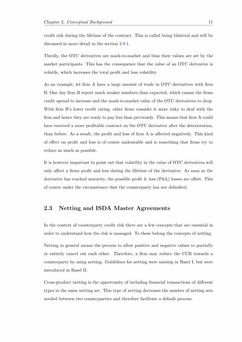
Figure 2.2: Example of netting 2 separate contracts

Chapter 2. Conceptual Background 13
Consider the example above with 2 separate contracts. Let the horizontal axis denote
time, and the vertical axis the CVA exposure of the contract. We see that during the first
period of time, contract No 1 has a positive exposure, and during the last period contract
1 has negative exposure. Contract No 2 has the opposite set up with negative exposure
during the first period, and positive exposure during the last period. If no netting would
be allowed, we would have a positive CVA exposure during the whole period of time.
On the other hand if netting is allowed, we see that the positive exposure from contract
No 1 is cancelled out by contract No 2’s negative exposure during that time. Similarly,
during the last period of time, where contract No 2’s positive exposure is cancelled out
by contract 1’s negative exposure. Hence, by allowing netting we obtain a zero value
CVA, instead of positive exposure during the whole period of time.
If a netting agreement is in place, the values of the contracts included in the agreement
are aggregated and the exposure is determined from the combined present value of
the netting set. Let K denote a netting set containing N trades. Mathematically, the
exposure of the netting is then given by
E(t) = max
{N∑i=1
Vi(t,T), 0
}. (2.1)
On the other hand, if no netting would be allowed, the exposure would be given by the
sum of the exposures on each trade determined by
E(t) = max {V (t,T), 0} . (2.2)
The effect of the netting set is seen from the inequality
max
{N∑i=1
Vi(t,T), 0
}≤
N∑i=1
max{Vi(t, T ), 0} (2.3)
where the expression on the left-hand side represents the exposure of a portfolio where
netting is allowed and the right-hand side represents the exposure of the same portfolio
without netting.
Chapter 2. Conceptual Background 14
2.4 Collateral and CSA
Just as with netting, collateral comes into scope within the context of mitigation of
CCR. To explain collateral in a simple way, let us consider a lender L and a borrower B.
L lends a sum of money in cash to borrower B. But, since L wants to be sure that the
cash is to be returned, B has to make a pledge of some asset to give up to L in case he
can not repay the cash. This asset that B promise L in the case of failure of payment is
called the collateral. With other words, collateral is the pledge of some specific property
from borrower to a lender, to secure repayment of a loan.
But what does collateral have to do with OTC derivatives and CVA? Collateral is not
just something that may be posted for loans. For an OTC derivative contract the
counterparties may also agree to post collateral under certain circumstances, in order to
reduce the counterparty risk. Hence, collateral is a tool that may be used to decrease the
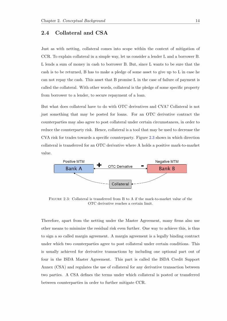
CVA risk for trades towards a specific counterparty. Figure 2.3 shows in which direction
collateral is transferred for an OTC derivative where A holds a positive mark-to-market
value.
Figure 2.3: Collateral is transferred from B to A if the mark-to-market value of theOTC derivative reaches a certain limit.
Therefore, apart from the netting under the Master Agreement, many firms also use
other means to minimize the residual risk even further. One way to achieve this, is thus
to sign a so called margin agreement. A margin agreement is a legally binding contract
under which two counterparties agree to post collateral under certain conditions. This
is usually achieved for derivative transactions by including one optional part out of
four in the ISDA Master Agreement. This part is called the ISDA Credit Support
Annex (CSA) and regulates the use of collateral for any derivative transaction between
two parties. A CSA defines the terms under which collateral is posted or transferred
between counterparties in order to further mitigate CCR.

Chapter 2. Conceptual Background 15
The CSA agreement may be either of bilateral or unilateral form depending on the di-
rection of the collateral posting. In a bilateral agreement, which is the most common
for derivative contracts, both counterparties can receive collateral. This type of agree-
ment is of course aimed to reduce the counterparty risk for both parties and is naturally
the most common type of agreement for OTC derivatives, since the value of these may
change sign as time goes by. However, in unilateral agreement only one predefined coun-
terparty has the right to receive collateral. One reason for this kind of agreement may
be the situation where all (or the vast majority) of the risk is carried by one party. This
form of agreement is less common for derivative contracts, according to [9], but common
for e.g. loans.
To summarize the last two sections, we see that there are ways to mitigate the credit
counterparty risk for OTC derivatives. But, due to the often complex nature of OTC
derivatives, the risk can never be fully removed on the counterparty level. To mitigate
the credit risk even further, a firm can utilize something called central counterparty
clearing. This term will be explained discussed in the next section.
2.5 Central counterparty clearing
Central counterparty (CCP) clearing has in the last few years begun to play an increas-
ingly important role in the OTC derivatives market, mainly due to the massive increase
the trade volume as described displayed in Figure 1.2. In its widest sense, clearing
denotes all activities from the time a commitment is made for a transaction until it is
settled and the delivery or exchange is made. CCP clearing is an activity performed by
a so called central counterparty clearing house. These are corporate entities who stand
between two counterparties in a trade and assumes the legal counterparty risk for the
firms involved. The counterparties of the contract in question are in this context called
clearing firms.
The CCP clearing house provides a guarantee to both clearing firms in a trade that if
one party defaults before the fulfilment of its obligations, the CCP fulfils the financial
obligations to the remaining party as agreed at the time of the trade. Because of the
large volume of trades that are carried out through a CCP, it often has the possibility

Chapter 2. Conceptual Background 16
of netting offsetting between counterparties to reduce the overall risk. The CCP usually
also use other means of reducing the risk, for example by:
� requiring collateral deposits,
� providing independent valuation of trades and collateral,
� monitoring the credit worthiness of the clearing firms and
� providing a guarantee fund that can be used to cover losses that exceed a defaulting
clearing firm’s collateral on deposit.
Derivatives that are cleared through CCPs are not included in the CVA calculation, since
the actual risk between the counterparties is neutralized. No matter what precautions a
CCP take in order to minimize the risks, there will always be a probability that it will
default. Therefore, to account for the still very unlikely event of a CCP default, Basel
III recognizes a risk associated even with cleared transactions. Generally it assigns a
risk weight of 2%, which should be held by the clearing firm.
Figure 2.4: Generally, the CVA may be mitigated by moving to collateralizationmethods more to the right in this graph. The best method being to use a CCP [10].
CCPs are present both in exchanges and in OTC markets. The process of transferring a
trade to a CCP clearing house is sometimes as quick as fractions of a second, but occa-
sionally it may take weeks. The time depends on the market liquidity of the instrument
traded, and largely upon the type of instrument.
As pointed in the beginning of this section, CCP clearing has become increasingly im-
portant due to the rapid growth in size of the OTC derivatives market. From the above
description it should clear what the advantages of cleared trades have in favour of the
non-cleared ones. But it is important to remember that the more customized and un-
common the derivative contract is, the more difficult it will be to transfer the trade to
a CCP. Hence, for some contracts it may take an unreasonably long time or even be
impossible to clear the trade through a CCP [8].

Chapter 2. Conceptual Background 17
Figure 2.5: The amount of transferred capital between counterparties may be sub-stantially reduced by using netting a agreements, and even further by using central
counterparty clearing.
2.6 Wrong way risk
Sometimes, the exposure a firm has towards a specific counterparty is co-dependent with
the credit rating of the counterparty. When this co-dependency is a negative correlation,
so that a larger exposure is correlated with a degraded credit rating it is called wrong
way risk (WWR). This type of relationship increases CCR and is highly undesirable for
any firm that has a will to survive.
Figure 2.6: Wrong way risk arises when a high exposure is correlated with a lowcredit rating towards a counterparty.
WWR is usually divided into specific and general WWR. Specific WWR arises when
the counterparty and guarantor of a transaction have a strong positive correlation. One
example would be when a firm uses its own shares as posted collateral for a transaction.
This is a bad idea since the firms disability to fulfil its obligations associated with the

Chapter 2. Conceptual Background 18
transaction is clearly positively correlated with drop in share value. The collateral will
drop when the share value does, and the exposure will increase.
General WWR is more subtle and therefore more difficult to avoid. This risk arises
where the credit quality of the counterparty may, for non-specific reasons be correlated
with macroeconomic factors that may also impact the exposure of transactions. The
guarantor may for example be in the same industry or located geographically close to the
counterparty. Another cause for general WWR would be if the guarantor has substantial
transactions with numerous firms in the same industry as the same industry. Market
factors affecting the firms in this industry will then indirectly influence the guarantor.
In practice, the exposure to a transaction and credit worthiness of counterparties are
usually measured and modelled independently. Especially, when calculating CVA, the
exposure is modelled as independent from the credit worthiness of a specific counterparty.
As a consequence, the wrong way risks become invisible in the CVA calculation. This is of
course a large drawback of CVA, but at the same time something that is extremely tricky
to avoid. Due to the innumerable possible wrong way risks for a specific transaction,
this type of risk is extremely difficult to estimate. Hence including all the dependencies
in a calculation would be almost impossible and moreover require immense amounts of
computer power. How wrong way risks are accounted for in one computation method is
seen in section 5.2.4.
2.7 CVA optimization
As we have seen in this chapter, there are many factors to take into account when
approaching counterparty credit risk and credit valuation adjustment. Many banks
have already invested significantly in order to build knowledge around these concepts
and some have also started to optimize their trading decisions with respect to CCR
and CVA. The concepts defined in this chapter constitute the basis for these trading
decisions. For example:
� How can the CCR be minimized by netting?
� Should collateral be posted?
� How should collateral be posted to minimize the risk?

Chapter 2. Conceptual Background 19
� Under what circumstances is it preferable trading through a CCP?
� How should wrong way risk be managed?
The truth is that these decisions are approached very differently by different firms. Some
use only netting to mitigate the CCR, while others also use collateral or trade through a
CCP. Wrong way risk may for example be tackled by an addition to expected exposure
or by a more sophisticated simulation of risk scenarios.
It should also be noted that are additional means of mitigating CVA that have not
been discussed in this chapter. Some examples are break clauses, novation and triRe-
duce. These are interesting risk mitigating techniques, but more detailed descriptions
are omitted here, since it lies outside the scope of this document.
But, regardless of how a firm is managing the CCR and mitigating CVA, questions
remain. What is the best way to measure the CVA, and is it possible to do quickly
considering all the complications involved in this measure? To answer these questions
we will introduce the regulatory methods to calculate CVA in Chapter 5.
2.8 Bilateral CVA
As explained above, both parties in an OTC derivatives contract will face a counterparty
credit risk. As a result, the CCR of both counterparties will be affected by an OTC
derivative contract. This means in a way that CCR is a bilateral risk (aside from the
unilateral credit risk).
An example of a bilateral risk could be illustrated by looking at an OTC derivative
contract. Let us consider one of the most common such contracts, namely the interest
rate swap (IRS). The IRS is a instrument in which the counterparties exchange interest
rate cash flows from a fixed rate to a floating rate, from a floating rate to a fixed rate,
or from one floating rate to another floating rate. Consider that bank A is paying the
floating leg and receiving the fixed leg. If the floating rate is larger the fixed rate at a
certain time t1, bank A has to pay more than it receives. So, at time t1 the contract has
a negative value and constitute a liability for bank A. If the floating rate at a later time
t2 drops below the fixed rate, then the bank recieves more than it pays. Hence, at this
point in time the contract has a positive value and is therefore an asset for bank A.

Chapter 2. Conceptual Background 20
As we can see in the above example, the CCR may move back and forth between the
counterparties during the lifetime of the IRS contract. The same is true for all OTC
derivative contracts, which clarifies the difficulty in assessing the CCR for these types
of contracts.
2.9 XVAs - Additional valuation adjustments
Throughout the last decades derivatives pricing has become increasingly complex, as-
suming a far greater significance than it previously had. Below we will treat the most
important valuation adjustments, the so called XVAs, with X denoting the type of value
of adjustment. These are a range of factors which may potentially cause banks quoting
different prices on the same contract.
It is almost always in the aftermath of a global financial crisis, banks realise that certain
assumptions that were taken for granted for many years needed to be reconsidered. Pre-
crisis, factors such as counterparty credit risk, funding risk and capital costs were hardly
considered when pricing derivatives, and the primary focus was to accurately price for
the market risk of the transaction.
However, the massively increased awareness of the importance of counterparty credit
risk has led to the development of a range of valuation adjustments. Unfortunately,
due to their recent introduction into the sphere, the understanding of these factors is
not very high and the required data in the calculations are not always easily accessible.
Hence the use of XVAs in derivatives pricing will most likely lead to pricing discrepancies
among quoting banks.
2.9.1 DVA - Debit valuation adjustment
The bilateral nature of CVA has brought a slightly controversial measure called debit
valuation adjustment (DVA) into the light of CCR. (Do not confuse with debt valuation
adjustment.) Imagine you are a bank, now DVA is the opposite of CVA, in the sense
that it reflects the credit risk your counterparty faces towards you. It is typically defined
as the difference between the value of the derivative assuming the bank is default-risk
free and the value reflecting default risk of the bank. Changes in a bank’s own credit

Chapter 2. Conceptual Background 21
risk therefore result in changes in the DVA component of the valuation of the bank’s
derivatives and thereby also affect the bilateral CVA against the counterparty.
There are several complications associated with isolating changes in the fair value of
derivatives due to changes in a bank’s own creditworthiness. DVA depend on the bank’s
own creditworthiness, the interest rate used for discounting and other drivers of the
expected exposure that the derivative creates for the counterparty. Therefore, DVA is
sensitive not only to changes in the own creditworthiness (i.e. credit spreads or proba-
bilities of default) but also to changes in all factors that affect the expected exposures.
The estimation of DVA, just as CVA, requires extremely complex modelling method-
ologies that estimate the evolution of exposures over time and rely on assumptions and
parameters that vary from bank to bank.
The main reason for the controversy around the DVA is the fact that credit rating drop
of a firm, will lead to MtM profits for the same firm. By increasing its own probability
of default and deteriorate in credit rating, a firm will experience a decrease in (bilateral)
accounting CVA. Let CV A1bi and CV A2
bi denote the bilateral CVA before respectively
after the drop in credit rating. The accounting CVA is calculated as unilateral accounting
CVA towards the counterparty, minus DVA as
CV A1bi = CV Auni −DV A. (2.4)
An increase in DVA (∆DV A) will hence induce a negative effect on CVA;
CV A2bi = CV Auni − (DV A+ ∆DV A) = CV A1
bi −∆DV A. (2.5)
For the firm in question, this means that the current outstanding OTC derivative trans-
actions have become less risky, and MtM values of the derivatives will rise. Whether or
not this is a reasonable and healthy reaction is debated. Nevertheless it is clear that
DVA is an important measure in the domain of counterparty credit risk, and that it will
remain in one form or another, as the CCR framework develops further. At the this of
writing it is mandatory for all banks to calculate DVA under a reporting standard called
IFRS 13: Fair Value Measurement, in effect since January 1st, 2013.

Chapter 2. Conceptual Background 22
2.9.2 LVA - Liquidity valuation adjustment
LVA - Liquid valuation adjustment is the discounted value of the difference between the
risk-free rate and the collateral rate paid (or received) on the collateral. It accounts for
liquidity related costs over the reference index that are not already accounted for by the
CVA. It is not appropriate to both use bilateral CVA and apply LVA based on market
funding rates. This would result in double counting. On the other hand, calculating
unilateral CVA and add LVA still makes sense. One can see LVA as the gain (or the loss)
produced by the liquidation of the net present value (NPV) of the derivative contract
due to the collateralization agreement.
2.9.3 FVA - Funding valuation adjustment
FVA - Funding valuation adjustment, refers to the funding consideration of the transac-
tion when the collateral type and terms on the client trade are not in line with collateral
type and terms of the market in which the bank will hedge the derivative. For example,
if the bank has to post cash collateral on the hedge and does not receive it in return
from the client, the bank would need to raise the cash itself as part of its usual funding
operations. Mathematically it is formulated as the discounted value of the spread paid
by the bank over the risk-free interest to finance the net amount of cash needed for the
collateral account and the underlying asset position. It can be seen as a correction or
residual made to the risk-free price of an OTC derivative to account for the funding cost
in an financial institution.
2.9.4 OCA - Own credit adjustment
Last but not least important in this section is the Own Credit Adjustment, OCA. Own
Credit adjustment is made to issue debt instruments accounted for, under the fair value
option to reflect the default risk of the entity. As a result of widening spreads during
the last years and the variability in these spreads, the own credit adjustment on issued
debt generates significant volatility in the income statement.
There is also an upcoming regulatory requirement to remove the variation of OCA from
Tier 1 capital. Under the new accounting standard , IFRS 9 Financial Instruments,

Chapter 2. Conceptual Background 23
which is expected to be in place by 2015, IFRS reporters will no longer record OCA in
the income statement. They will instead record the OCA under Other Comprehensive
Income (OCI), within sharholders’ equity. OCA measurement is a high point of focus
for banks as a result of the materiality of the credit adjustment, the volatility and the
communication challenges. The method for calculating OCA can be of different nature.
The four most common methods are using the following curves, target funding curve,
CDS curve, secondary market data curves (bond spreads and levels of buybacks etc) and
primary issuance data.

Chapter 3
Mathematical Definitions
In this chapter we will walk through some of the most important mathematical inputs
when calculating credit value adjustment, CVA.
3.1 PV - Present value
When computing the CVA, a large amount of values need to be included to get a proper
valuation. One of the most basic of these is the present value (PV). It is also known
as present discounted value and is a amount of future money that has been discounted
to reflect its current value, as if it existed today.The present value is always less than
or equal to the future value, because money has an interest-earning potential. This
characteristic is often referred to as the the time value of money. The present value
depends on the type of contract in question, and it is determined by market and credit
risk factors. The present value at an arbitrary time t ≥ 0 is given by the expected value
of the discounted dividend under a risk neutral measure. The present value at time t is
often denoted V(t,T),
V (t, T ) = E
∑u∈(t,T ]
C(u)D(t,u)
. (3.1)
Where
24

Chapter 3. Mathematical Definitions 25
D(t,u) is the discount factor between the times t and u,
C(u) is the dividend or payout at time u,
T the time of maturity of the contract,
u may assume discrete time points in the interval (t,T].
3.2 Exposure
The exposure of a contract is by definition the amount that one stands to lose in an
investment in case of a default by a counterparty. The exposure depends on whether
the contract is a liability or an asset. If the contract has a negative present value it is a
liability to the investor, and hence the investor has the obligation to pay the value to the
counterparty. In case of counterparty default this amount is still due and has to be paid
to the creditors of the defaulted company. If the contract has a positive present value,
it is an asset of the investor that is to be received from the counterparty. In case of a
counterparty default this value will not be paid out in its full amount and the exposure
is hence equal to the present value. Thus, the exposure is equal to the present value if
it is positive and zero otherwise
E(t) = max(V(t,T), 0). (3.2)
3.3 PD - Probability of Default
Probability of Default (PD) is a financial term describing the credit-worthiness of a
counterparty. It explains the likelihood of a default over a particular time horizon,
often a year and is expressed as a Probability Density Function (PDF), which assigns
probability mass to time points by the associated Cumulative Distribution Function
(CDF). The Probability of Default can be estimated for a particular obligor which is
the usual practice in wholesale banking, or for a segment of obligors sharing similar
credit risk characteristics which is the usual practice in retail banking. The Probability
of Default is a key parameter used in the calculation of economic capital or regulatory
capital under Basel II for a banking institution. Should the borrower be unable to pay,
they are then said to be in default of the debt, at which point the lenders of the debt
have legal avenues to attempt obtaining at least partial repayment. Generally speaking,

Chapter 3. Mathematical Definitions 26
the higher the default probability a lender estimates a borrower to have, the higher
the interest rate the lender will charge the borrower (as compensation for bearing higher
default risk). The great importance of estimating the Probability of Default is in gaining
a good comprehension of a specific obligor’s credit quality. By making a comparison
between the real and the estimated defaults, it is possible to see different properties over
one business cycle or more. The Probability of Default of an obligor not only depends on
the risk characteristics of that particular obligor but also the economic environment and
the degree to which it affects the obligor. Thus, the information available to estimate
Probability of Default can be divided into two broad categories
� Macroeconomic information like house price indices, unemployment, GDP growth
rates, etc.
� Obligor specific information like revenue growth, number of times delinquent in
the past six months etc.
3.4 LGD - Loss Given Default
There is a broad market interest in disaggregating the components of credit risk. One
of the major components is the Loss Given Default or LGD term. It is a common
parameter in Risk Models and also a parameter used in the calculation of Economic
Capital or Regulatory Capital under Basel II for a banking institution. This is an
attribute of any exposure on a bank’s client. LGD is percentage of loss over the total
exposure when bank’s counterparty goes to default. The amount of funds that is lost by
a bank or other financial institution when a borrower defaults on a loan. Theoretically,
LGD is calculated in different ways, but the most popular is ’Gross’ LGD, where total
losses are divided by exposure at default (EAD). Another method is to divide Losses
by the unsecured portion of a credit line (where security covers a portion of EAD).
This is known as ’Blanco’ LGD. If collateral value is zero in the last case then Blanco
LGD is equivalent to Gross LGD. Among banks, the Blanco LGD is popular because
banks often have many secured facilities, and banks would like to decompose their losses
between losses on unsecured portions and losses on secured portions due to depreciation
of collateral quality. The most popular method among academics though, is the Gross

Chapter 3. Mathematical Definitions 27
LGD because of its simplicity and because academics only have access to bond market
data, where collateral values often are unknown, uncalculated or irrelevant
3.5 EAD - Exposure at Default
It is of great interest to all financial institutions to control the Exposure at Default.
The EAD is along with loss given default,(LGD) and probability of default, (PD) used
to calculate the credit risk capital of financial institutions. In general, it is seen as an
estimation of the extent to which a bank may be exposed to a counterparty in the event
of a possible default. Exposure at Default is calculated through different methods which
we will describe more proper in chapter 5. Two of the most common methods are the
Current Exposure Method (CEM) and the Standard Method (SM)

Chapter 4
Regulations
Throughout the history, regulations have always been a part of the financial market.
It started to grow in the early 20th century. The practice of investing was being kept
mostly among the wealthy, who could afford to buy into joint stock companies and
purchase debt in the form of bank bonds. It was believed that these people could handle
the risk because of their already considerable wealth base. The level of fraud in the
early financials was enough to scare off most of the casual investors. As the importance
of the financial market grew, it became a larger and larger part of the overall economy
in the U.S., thus becoming a greater concern to the government. Investing grew quickly
as all classes of people began to enjoy higher disposable incomes and finding new places
to put their money. In theory, these new investors were protected by the Blue Sky Laws
(first enacted in Kansas in 1911). These state laws were meant to protect investors from
worthless securities issued by unscrupulous companies and pumped by promoters. They
are basic disclosure laws that require a company to provide a prospectus in which the
promoters can rely on. In this chapter we will treat the most important regulations
concerning credit value adjustment.
4.1 Basel II
Basel II was initially published in June 2004 and was intended to create an international
standard for banking regulators to control how much capital banks need to put aside to
guard against the types of financial and operational risks banks face in their daily work.
28

Chapter 4. Regulations 29
It was the second of the Basel Committee on Bank Supervisions recommendations,
and unlike the first accord, Basel I, where focus was mainly on credit risk one now
tried to move the risk awareness a few steps further. Basel II tries to integrate Basel
capital standards with national regulations, by setting minimum capital requirements of
financial institutions to ensure that a bank has adequate capital for the risk the bank
exposes itself to through its lending and investment practices. Politically, it was difficult
to implement Basel II in the regulatory environment prior to 2008, and progress was
generally slow until that years of the banking crisis. Today we know that the divisions
of risk handling at the financial institutions are far more developed.
Basel II is based on three pillars.
The first pillar deals with maintenance of regulatory capital calculated for the three
major components of risks that a bank faces which are credit risk, operational risk
and market risk. The second pillar is a regulatory response to the first pillar. It also
provides a framework for dealing with systemic risk, strategic risk, liquidity risk etc. It
is the International Capital Adequacy Assessment Process (ICAAP) which is the result
of Pillar II of Basel II accords. The third pillar aims to complement the minimum
capital requirements and supervisory review process by developing a set of disclosure
requirements which will allow the market participants to gauge the capital adequacy of
an institution. Under Basel II, the risk of counterparty default and credit migration risk
were addressed but mark-to-market losses due to CVA were not. This was a big problem
and was taken into account under development of Basel III.
4.2 Basel III
During late 2009, the Basel Committee on Banking Supervision published the the first
version of Basel III, giving banks approximately three years to satisfy all requirements.
In September 2010, global Banking regulators sealed a deal to effectively triple the size
of the capital reserves that the world’s banks must hold against losses. It sets a new
capital key capital ratio of 4.5%, more than double the today 2 per cent level, plus a
new buffer of 2.5%. The new rules will be phased in from January 2013 to January
2019, where the minimum Liquidity Coverage Ratio (LCR) requirement in 2015 is 60%,
and then adding on 10% each year to reach 100% LCR in 2019. Basel III is part of the

Chapter 4. Regulations 30
continuous struggling effort to enhance the banking regulatory framework. It is build
on Basel I and Basel II documents, and seeks to improve the banking sector’s ability to
deal with financial and economic stress, improve risk management and strengthen the
banks transparency.
Basel III is also based on 3 pillars
First it is the minimum capital and liquidity requirements in the division for credit risk,
market risk and operational risk. The second pillar is the supervisory review process
which include regulatory framework for banks and supervisory framework. The third
pillar cover the market discipline and disclosure requirements of banks. Basel III has an
impact on several areas. When addressing it to CVA we see that most of the impact is
related to infrastructure, data management and regulatory reporting. Calculating CVA
for a counterparty will need huge amounts of historical data, which may require the use
of new data marts and data bases. It will also affect the existing reports which will be
used to reflect CVA besides new capital structure.
4.3 CRD IV and CRR
The European Commission’s proposals divide the current Capital Requirements Direc-
tive (CRD) into two legislative instruments: the Capital Requirements Regulation (the
CRR) and the CRD IV Directive. The CRR contains provisions relating to the “single
rule book”, including the majority of the provisions relating to the Basel III pruden-
tial reforms while the CRD IV Directive introduces provisions concerning remuneration,
enhanced governance and transparency and the introduction of buffers.
Like the current CRD, the CRR and the CRD IV Directive will apply to credit insti-
tutions and to investment firms that fall within the scope of the Markets in Financial
Instruments Directive. In line with Basel III, the CRD IV proposals create five new
capital buffers: the capital conservation buffer, the counter-cyclical buffer, the systemic
risk buffer, the global systemic institutions buffer and the other systemic institutions
buffer.
CRD IV is binding on all EU member states. It aims to address the problems that
caused the financial crisis by increasing the level and quality of capital held by banks,

Chapter 4. Regulations 31
enhancing risk coverage, expanding disclosure requirements and reducing procyclicality.
CRD IV provides a basis for EU liquidity standards and introduces leverage disclosure
requirements. It also places greater emphasis on the highest quality of capital (known
under CRD IV as Core Equity Tier 1) than the current regime and strengthens the
criteria used to determine what can be used as CET1. CRD IV consists of a directly
applicable EU Regulation, and an EU Directive which must be reflected in national law.
The bulk of the rules contained in the legislation will apply from 1 January 2014.
The actual impact of CRD IV on capital ratios may be materially different as the re-
quirements and related technical standards have not yet been finalised, for example
provisions relating to the scope of application of the CVA volatility charge and restric-
tions on short hedges relating to insignificant financial holdings. The actual impact
will also be dependent on required regulatory approvals and the extent to which further
management action is taken prior to implementation
4.3.1 LCR - Liquidity Coverage Ratio and NSFR - Net Stable Funding
Requirement
The CRR part of CRD introduces two new liquidity buffers:
� Liquidity Coverage Requirement (LCR) which is intended to improve short term
resilience of the liquidity risk profile of firms
� Net Stable Funding Requirement (NSFR) which is intended to ensure that a firm
has an acceptable amount of stable funding to support its assets and activities
over the medium term
The LCR is designed to measure whether firms hold an adequate level of unencumbered,
high-quality liquid assets (HQLA) to meet net cash outflows under a stress scenario
lasting for 30 days. These papers shall be so liquid that can be converted easily and im-
mediately in private markets into cash to meet their liquidity needs. The LCR measures
the stock of liquid assets against net cash outflows arising in the 30 day stress scenario
period. The LCR will improve the banking sector’s ability to absorb shocks arising from
financial and economic stress, whatever the source, thus reducing the risk of spillover
from the financial sector to the real economy. Firms would be expected to maintain an
LCR of at least 100 per cent. Under the CRR the LCR will be implemented faster than
Chapter 4. Regulations 32
originally envisaged under Basel III. The timetable will be: 60 per cent in 2015, 70 per
cent in 2016, 80 per cent in 2017 and 100 per cent in 2018. During a period of financial
stress, however, banks may use their stock of HQLA, thereby falling below 100%, as
maintaining the LCR at 100% under such circumstances could produce undue negative
effects on the bank and other market participants.
Whilst the LCR will be introduced from 2015 the CRR establishes a general requirement
that firms need to hold liquid assets to cover their net cash outflows in stressed conditions
over a 30 day period. However, this is a general requirement and not a detailed ratio
requirement.
The Net Stable Funding Ratio (NSFR) is as the name describes it, a landmark require-
ment that will apply to all banks worldwide to ensure a more stable and robust funding.
It has also been proposed within Basel III.
� Stable funding includes: customer deposits, long-term wholesale funding (from the
Interbank lending market) and Equity
� Stable funding excludes: short-term wholesale funding (also from the Interbank
lending market)
Together with the liquidity coverage ratio (LCR), the Net Stable Funding ratios (NSF
ratios) are part of the new proposed development of international liquidity standards.
Banks have until until 2018 to meet the NSFR standard. Over time this Net Stable
Funding ratio will be reviewed as proposals are developed and industry standards im-
plemented
4.3.2 HQLA - High Quality Liquid Asset
When talking about LCR, you always have to include HQLA, High Quality Liquid Asset.
Under the standard, banks must be able to hold a stock of unencumbered HQLA to cover
the total net cash outflows over a 30-day period under the prescribed stress scenario.
Assets are considered to be HQLA if they can be easily and immediately converted into
cash at little or no loss of value. The liquidity of an asset depends on the underlying
stress scenario, the volume to be monetised and the time frame considered. There are a
few fundamental market characteristics that must be fulfilled to be called a HQLA.

Chapter 4. Regulations 33
Fundamental characteristics
� The asset shall be of low risk, as they then tend to have higher liquidity. High
credit standing of the issuer and a low degree of subordination increase aswell an
asset’s liquidity
� The asset’s valuation shall be of great certainty. The asset’s liquidity increases if
market participants are more likely to agree on its valuation. Assets with more
standardised,homogenous and simple structures tend to be more fungible, promot-
ing liquidity
� The asset must have low correlation with risky assets, for example assets issued
by financial institutions are more likely to be illiquid in times of liquidity stress in
the banking sector
� The asset shall be listed on a true developed and recognized exchange
4.4 Regulations of OTC instruments
Regulations on OTC derivative trading is planned to be implemented in the near fu-
ture. The Markets in Financial Instruments Directive II (MiFID II) currently has an
implementation time set to 2014/2015 and will among other things force firms to clear
”some” derivative trades through CCP clearing houses. With ”some”, it is meant the
derivatives with a sufficient market liquidity. Further, MiFID introduces a new type
of CCP trading platform called organized trading facility (OTF) which will act as an
intermediary for the clearing firms.

Chapter 5
Regulatory Methods
5.1 Introduction to Regulatory Methods
5.1.1 Regulatory separation of risks
Counterparty credit risk is under Basel divided into two kinds of risks.
1. The risk associated with the default of counterparties.
2. The risk of mark-to-market losses on the expected counterparty risk.
The former type of risk is credit risk while the latter is the one associated with as CVA
and the type of risk that this document is more focused on. It is also this one that is
more complex of the two. Note however that the second type of counterparty credit risk
depends on the probability of default of counterparties, and we will therefore examine
the counterparty default risk as well. Later in this chapter the dependence between the
two is clarified. Under the Basel II framework, a two-step process is followed to compute
the required capital for counterparty credit risk.
1. The risk weight of the counterparties must be calculated.
2. One must calculate the credit exposures arising from bilateral transactions. This
is, calculating the measure called exposure at default (EAD).
The measure EAD recur in the calculation of CVA capital, as we shall see later in this
chapter. We shall now proceed by taking a look at risk weights in its most general form.
34

Chapter 5. Regulatory Methods 35
5.1.2 RWA - Risk-weighted assets
Risk-weighted assets (RWA) was introduced under the first Base accord as a measure
of a financial institutions minimum capital requirements. The CVA was introduced as
a part of the RWA, under the Basel III Accord. RWA is thus a very broad measure of
risk capital, containing a CVA and many other capital requirements. In this document,
our intention is just to briefly explain RWA so that the reader may understand how it
is related to CVA. RWA is computed by adjusting each asset class with a certain weight
depending on the risk associated with the specific asset class. The weight is supposed to
account for all types of risks faced by a firm; market, credit and operational risks. Under
the Basel III accord, a bank must have top quality (Tier 1) capital equivalent to at least
seven percent of RWA. Otherwise it faces possible restrictions on paying bonuses, as
well as dividends to shareholders. The new rules are being phased in from January 2013
through to January 2019. Tier 1 capital is a regulatory measure of a firms core capital
consisting of primarily common stock and disclosed reserves.
5.1.3 Regulatory approaches to credit risk
In order to clarify any confusion regarding the different methods for calculating risks
under Basel, this section is dedicated to the credit risk calculation approaches, and shall
not be confused with the methods for calculating counterparty credit risk. Note however
that some of the components are shared between these two different risk types. Recall
that the first step in computing capital requirements for credit risk is to calculate the
risk-weights of the transactions against every counterparty. There exist a few different
methods to compute these weights used in the calculation of the regulatory credit risk
capital. These are divided into
1. The standardized approach (not to confuse with standardized approach under
CCR)
2. The internal ratings-based (IRB) approach.
Under the standardized approach, financial institutions are required to use the risk
weights supplied by regulators for estimation of the capital requirement. No approval
from the regulators are needed for using of this method.

Chapter 5. Regulatory Methods 36
The internal ratings-based approach is divided into one so called foundation IRB ap-
proach and one advanced IRB approach. Foundation internal ratings based approach
(F-IRB) is a method for financial institutions to calculate credit risk components, intro-
duced under Basel II. The approach allows firms to estimate the probability of default
(PD) for certain counterparties. Other parameters needed to calculate risk weighted
assets must be computed using methods prescribed by regulatory authorities. As a con-
sequence, exposure at default (EAD) and loss given default (LGD) must be computed
via these regulatory methods.
Advanced internal ratings-based (A-IRB) approach is a method for financial institutions
to calculate credit risk components internally which was introduced under Basel II. It
allows institutions to calculate risk components themselves, that would otherwise be
estimated by regulatory authorities. Banks need an approval in order to use the A-IRB
approach. One reason why a firm would prefer to calculate risk internally to a larger
extent is that the risk components calculated by regulatory authorities often are not
as precise and therefore necessarily more conservative. Additional risk measures that
may be calculated under A-IRB include probability of default (PD), exposure at default
(EAD), loss given default (LGD).
In the next section we will leave the more general Basel frameworks and credit risk
behind us, and dive into the regulatory methods of counterparty credit risk and credit
valuation adjustment.
5.1.4 Regulatory CVA methods
The CVA capital charge is calculated depending on the bank’s approved method;
1. for calculating counterparty credit risk (i.e. if it has IMM approval) and
2. using a VaR model for bonds to model credit spreads and default probabilities
The assessment of exposure at default for derivative transactions depends on several
factors, which are described in Chapter 2. Recall that to these belong the bilateral
nature of derivative transactions, fluctuations in market risk factors, netting sets and
collateral agreements.

Chapter 5. Regulatory Methods 37
Firms can currently choose from two distinct approaches to calculate the CVA for OTC
derivative transactions. These are called the standardized and the advanced approaches.
Note that the standardized approach in this context has no connection to the standard-
ized approach in a credit risk context. In this document we will refer to the one method
used in the advanced approach as the advanced method (AM). Moreover, under the stan-
dard approach, regulatory CVA capital can be calculated using three different methods.
The main difference between the three standardized methods for the regulatory CVA
capital calculation lies in how they compute EAD. One of these is a so called internal
model method (IMM), requiring a certain approval from supervisory authorities. The
two other are so called non-internal model methods (non-IMM), with different degrees
of complexity; the current exposure method (CEM) and the standardised method (SM).
Figure 5.1: The two approaches and four different methods for calculating the CVAcapital requirement.
A graphical representation of the approaches and methods is shown in Figure 5.1 above.
The advanced method calculates CVA through simulations of credit spreads for each
counterparty. The other three (current exposure, standardized and internal model)
methods compute the CVA of the netting sets described in Section 2.3. The netting set
CVA contributions can thereafter simply be summed up to form the aggregate CVA.
Banks with no approvals for capital charge calculations may use the standardised or
current exposure methods. Banks with approval for internal counterparty credit risk
model (IMM approval) may use the internal model method. Furthermore, banks with
approval both for a internal CCR model (IMM approval) and simulation of counterparty
default probabilities, may use the advanced method. We will not go into details on
reasons or requirements of obtaining the IMM approval here, but some aspects of it is
covered in Section 7.2.

Chapter 5. Regulatory Methods 38
Note that a bank may have IMM approval for calculating CCR only towards certain
counterparties or for certain transactions. Then for example the internal model method
may be used on the approved transactions, while a non-internal method must be used
on the remaining. In the next section all these different methods will be described in
much more detail.
5.2 Standardized Approach
The standardized approach for calculating CVA under the Basel accord is derived from
a VaR formulation of CVA, but simplified under a set of assumptions. The list of
assumptions used here is taken from a document at the Federal Register [13].
� Credit spreads have a flat term structure (i.e. spreads are independent of tenor).
� Credit spreads are log-normally distributed.
� Single name credit spreads are driven by the combination of a systematic (market)
risk factor and one idiosyncratic risk factor. Idiosyncratic meaning a factor which
only affects a small group of assets.
� The correlation between any single name credit spread and the systematic risk
factor equals 0.5.
� All credit indexes are driven by the single systematic factor.
� The time horizon is short.
An approximation is achieved by linearization of the dependence of both CVA and CDS
hedges on credit spreads. This together with the the above simplifications, makes it
possible to express VaR of CVA explicitly in an analytical formula. As we shall see
later in this section, certain further simplifications and conservative adjustments are
made to the CVA measure, depending on the actual methodology used. The formula for
calculating regulatory CVA (KstdCV A) under the standardized approach is,
KstdCV A =2.33
√H ×
√√√√(1
2
∑i
wiΛi −∑ind
windMeindBind
)2
+3
4
∑i
w2i Λ
2i , (5.1)
Λi =M ei EADi −M eH
i Bi,
and where the following are the variables used;

Chapter 5. Regulatory Methods 39
wi Weight (concretization of counterparty rating) of counterparty i
M ei Effective maturity for netting set of counterparty i
M eHi Effective maturity of single name hedge towards counterparty i
EADi Exposure at default of counterparty i
Bi Notional of single name hedge towards counterparty i
wind Index hedge weight
M eind Maturity adjustment factor for index hedge
Bind Notional of index hedge
Note that Λi represents the non-netted but possibly hedged exposure of transaction i.
The weights (wis) used in the formula can be obtained from Table 5.1 below.
Rating AAA AA A BBB BB B CCC
Weight×100 0.7 0.7 0.8 1.0 2.0 3.0 10.0
Table 5.1: Correspondence between counterparty rating and CVA weight accordingto Basel III.
Basel III introduced a discount factor which is multiplied by each component of exposure
at default (EADi) and hedge notionals (Bi and Bind) to produce the discounted values
which are used in the CVA capital calculation (5.1). The discount factor used is given
by
DF =
(1− e−0.05·Mι
0.05 ·Mι
), (5.2)
where ι may take the value i or ind.
To get a better understanding of the standardized CVA formula, let us look at (5.1) in
the case where hedges are excluded (Bi = 0 ∀i and Bind = 0 ∀ind). Inserting Λi gives,
KstdCV A =2.33
√H ×
√√√√(1
2
∑i
wiM ei EADi
)2
+3
4
∑i
w2i (M e
i EADi)2
=KstdCV A = 2.33
√H ×
∑i
wiMei EADi (5.3)

Chapter 5. Regulatory Methods 40
Equation (5.1) may be written on the more compact form
KstdCV A = Φ−1(q)
√Hβ, (5.4)
using the notation
Φ the standard normal cumulative distribution function,
q confidence level, which in this case is 99%.
We have that Φ−1(0.99) ≈ 2.33 and that β is given by the expression
β2 =
[1
2
∑i
wiΛi −∑ind
windMeindBind
]2+
3
4
∑i
w2i Λ
2i , (5.5)
Λi =M ei EADi −M eH
i Bi.
For institutions using (5.1) to calculate the capital charge it may of course be interesting
to know where this equation comes from. From the inverse standard normal distribution
existing in (5.4) it may be suggested that the expression represents a certain value at
risk with confidence level 99% and time horizon H years. This is actually also the case,
although it is actually not explicitly stated in the Basel Accord. To motivate the use of
the CVA capital charge for the rigorous reader, a derivation of it is found e.g. in [6].
For all the methods under the standardized approach, equation (5.1) is used to calculate
the CVA amount. The difference between the methods lies in how the exposure at
default (EAD) and effective maturity (M e) are computed. In the next sections, the
different methods under the standardized approach will be gone through.
5.2.1 SM - Standardized Method
The standardized method is defined in section VI, Annex IV of the Basel II accord.
Currently, very few financial institutions use SM to estimate exposure at default to
counterparties and the number does not seem to be increasing [18]. Moreover, there is
a substantial loss in documentation concerning the method. Due to this fact, we will
deliberately not cover the mathematical details of the standardized method, but rather
just give a short summary of how it is used to compute exposure at default.

Chapter 5. Regulatory Methods 41
Exposure at default
Under the standardized method, exposure at default is calculated for separate so called
hedging sets. A hedging set is defined as transactions that share the same market risk
factors. Provided that transactions in the same hedging set also are in the same netting
set, they are able to offset each other. When computing the exposure for a hedging set,
this exposure is never less than the current MtM value of the netting set. The use of
hedging sets has the advantage that it makes possible calculation of the value of the
delta hedge that would offset the position. Hence, in order to compute the exposure,
each leg of the transaction is first expressed as a delta-equivalent notional. In the SM,
no diversification benefit is obtained across the hedging sets, since each set is considered
to be independent of the others.
5.2.2 CEM - Current Exposure Method
Exposure At Default
The current exposure method is defined in section VII, Annex IV of the Basel II accord.
CEM is, at the moment of writing, the by far most common method for computing EAD.
In this method, the EAD is computed as a sum of three terms. The first term represents
the current value of the exposure is calculated as the current positive mark-to-market
value. The second term is an add-on which accounts for the probability of an increased
exposure due to market movements or changed volatility in the underlying. The value
of this term is set so that there should be only a certain very small probability that it
is exceeded. The third term is the volatility adjusted amount of collateral.
Let us consider a the exposure of default of a single transaction i (EADi), under CEM.
EADi is defined as the current exposure of the transaction (CEi) plus the additional
potential future exposure (PFEi) minus collateral posted by the counterparty (CAi ).
The convention is to set a minus in front of the collateral term and thus consider a
positive CAi . The expression using the method for one single transaction is,
EADi = CEi + PFEi − CAi . (5.6)

Chapter 5. Regulatory Methods 42
As said above, first term (CEi) represents the current value of the exposure is calculated
as the current positive mark-to-market value,
CEi = max (0,MTMi) . (5.7)
One term needed in the calculation of the exposure at default is the credit conversion
factor (CCF ). This factor depends on the kind of contract in question and the maturity
of the contract. It reflects the potential future change in contract value between the
date of calculation and the date at which the contract should be able to be replaced or
closed out in the case a counterparty default. CCF was first introduced under Basel II
and its values are shown in the table below [12, p. 6].
````````````````````Contract type
Time to Maturity< 1 year 1− 5 year > 5 year
Interest rate 0.0 0.5 1.5
Foreign exchange and gold 1.0 5.0 7.5
Equities 6.0 8.0 10.0
Precious metals except gold 7.0 7.0 8.0
Other 10.0 12.0 15.0
Table 5.2: Credit conversion factors (CCFs) for different contract types and maturi-ties. All factors are given in percent (%).
PFE is made up of the contract notional amount (Ni) multiplied by the credit conversion
factor from Table 5.2. For example, for a single contract we can write it as
PFEi = Ni · CCFi. (5.8)
Using the above notation we arrive at the full expression for EAD under CEM for a
single transaction,
EADi = max (0,MTMi) +Ni · CCFi − CAi . (5.9)

Chapter 5. Regulatory Methods 43
Netting under CEM
When considering a netting set with multiple transactions we must also take netting
between transactions into account in the computation of EAD. The potential future
exposure term PFE is in this case the netted aggregate potential future exposure of the
netting set.
PFE = ([1− ρ] + ρ ·NGR)∑i
PFEi. (5.10)
The PFE term may be netted up to a certain amount ρ depending on the current
netting of the mark-to-market value within the corresponding netting set. The value of
ρ represents the correlation between transactions that share netting set and satisfies 0 ≤
ρ ≤ 1. When CEM was first introduced in Basel, the value was set very conservatively
to ρ = 0.6. This has later been changed and now is set to a more realistic value of 0.85.
The netting is computed by a term called net-to-gross ratio (NGR - sometimes ”net
current replacement cost to gross current replacement cost”),
NGR =max (
∑ni=1MtMi, 0)∑n
i=1 max(MtMi, 0). (5.11)
NGR here acts as a proxy for the impact of netting on potential future exposure. NGR
may be strongly effected by idiosyncratic factors, since the transactions that share net-
ting set usually are strongly correlated. This means that NGR is not a particularly
precise indicator of net to gross exposure ratio [12].
So, how does the NGR depend on the mark to market values of the contracts? We
see that if all MtM values are non-negative then the numerator and denominator will
be equal and the NGR will have a value of one. This is the worst possible scenario in
means of exposure for a firm. On the other extreme, if none of the MtM values are
positive, then both numerator and denominator will be zero. This is an especially nasty
expression, and it is a bit odd that this expression is allowed. However, one may observe
that the more of the terms that are negative, the smaller will NGR be, due to terms
cancelling out in the numerator. E.g., if at least half the total MtM value is negative,
then NGR will have a value of zero (if at least on MtM value is positive).
As a method to assess CCR, the current exposure method is an approximation method,
which is not certain to reflect the real risk especially well. As a consequence of this,
netting of positions and the use of collateral give only partial risk mitigation using

Chapter 5. Regulatory Methods 44
CEM. This makes the CEM a rather conservative method in comparison to the other
ones, which becomes obvious looking at the tests Section 7.1.
Effective Maturity under CEM
Effective maturity of counterparty i (M ei ) is according to the CEM calculated by (5.12)
[19]. The equation represents the weighted average of all remaining maturities on con-
tracts towards counterparty i. If there exist more than one netting set to the same
counterparty, effective maturity should be computed separately for each netting set.
The floor (minimum value) of the effective maturity is set at 1 year. Earlier, there was
also a cap (maximum value) set at 5 years, but this was removed in a Basel III update in
June 2011. The reason for removing the cap is to better capture the risk associated with
transactions with a long maturity. The equation for determining the effective maturity
is given by
M ei = max
(1,
∑jMi,jNi,j∑j Ni,j
), (5.12)
using the notation
Mi,j Maturity of contract j towards counterparty i,
Ni,j Notional of contract j towards counterparty i.
The more advanced internal model methods for computing CVA will be described in
the next section. As we shall see, the non-internal model approach has some significant
shortcomings in comparison to the internal methods.
5.2.3 A note on future non-internal model methods
The Basel Committee on Banking Supervision published on 28 June 2013 a paper in
which they propose to revise the current non-internal model methods SM and CEM.
Both models are planned to be replaced by a single new method under the name non-
internal model method (NIMM). The proposed method is said to be more risk sensitive
than both SM and CEM and shall address some of the criticism than has been aimed at
these methods since they were first introduced. One point of criticism of the methods is

Chapter 5. Regulatory Methods 45
the poor support for risk mitigation from collateral agreements. Further, the net-to-gross
ratio is often considered to be over-simplistic and not to reflect netting properly.
In other words, it seems as if NIMM will replace SM and CEM in a not to distant future.
This is everyday news in the financial industry. Regulations and models change all the
time, and banks are in a constant struggle to adapt to the next alteration in the financial
environment. But no matter how soon in the future the financial framework will be ,
it is utmost importance for financial institutions to have a solid understanding of the
current framework.
5.2.4 IMM - Internal Model Method
The internal method model is a way to compute CVA for firms that have a regulator
approved model for CCR, so called IMM approval.
According to a report from Deloitte released February 2013 [11] an increasing number
of banks internationally are using IMM as the way to calculate regulatory CVA capital.
The reason for this is said to advocate that in practice the results obtained from using
IMM is superior to CEM. However, some exotic derivates are usually valued using a semi-
analytical approach, which demand the use of CEM rather than IMM for computing the
exposure at default.
Exposure At Default under IMM
To fully understand how EAD is calculated using the internal model method, we first
need to define a few concepts on whom the calculation is based. Firstly, let us consider
a bank which has a portfolio of contracts towards a single counterparty i. Now the
exposure towards this counterparty at time t is denoted Ei(t). This value depends on
the MTM value of the portfolio (Vi(t)) and the amount of collateral (Ci(t)) available at
time t, according to
Ei(t) = max{Vi(t)− Ci(t), 0}. (5.13)
EE - Expected Exposure
It is important to note that the portfolio value in (5.13) is the risk free value from the
perspective of the bank. Also note that a positive Ci(t) implies that the bank holds
Chapter 5. Regulatory Methods 46
collateral and a negative means that the bank has posted collateral at time t. The
notation of the expected exposure (EE) against counterparty i at time t is then given
as
EEi(t) = E [Ei(t)] . (5.14)
EPE - Expected positive exposure
Usually time dimension is discretized into a fixed number of time points tk in order
to represent the expected values as a functions of time. The expected values are then
computed by simulations of future exposures at every time step. The expected positive
exposure (EPE) is defined as the average of the EE over a specific time horizon denoted
H;
EPE =1
H
∑tk≤H
EE(tk)∆tk. (5.15)
EEE - Effective expected exposure
The effective expected exposure (EEE) is defined as the non-decreasing expected expo-
sure with respect to time, according to
EEE(tk) = max{EEE(tk−1), EE(tk)}. (5.16)
EEPE - Effective expected positive exposure
We are now prepared to define the factor which we need in order to understand how
exposure at default is calculated under IMM. This is effective expected positive exposure
(EEPE), and it is defined as the one year average of the EEE
EEPE =1
H
∑tk≤H
EEE(tk)∆tk. (5.17)
EAD - Exposure at default
Having arrived at the expression for effective expected positive exposure we are now
ready to give the expression for EAD under the internal model method. EAD is calcu-
lated as the product of a multiplier alpha and EEPE as in (5.18),
EAD = α · EEPE. (5.18)

Chapter 5. Regulatory Methods 47
The EEPE is generated via a Monte Carlo model which must be approved by regulators.
At least three years of historical data must be used in the Monte Carlo model, whereof
one year must be from a so called ”stressed” scenario. With a stressed scenario is
meant from periods with unusually unstable economical conditions and increased credit
spreads.
Unlike the current exposure method, the internal model method allows future collateral
to be included in the risk capital calculation. But firms need approval specifically for a
collateral model in order to get the full risk mitigation [19]. Unfortunately however, we
will not have the opportunity of looking further into the effects of collateral on the CVA
capital charge in this document.
α
The alpha multiplier is formally defined as the ratio between economic capital (as com-
puted with the full IMM) and one calculation carried out with deterministic exposures
set to EPE. The existence of the alpha is meant to account for wrong way risks (WWRs)
and other model issues. To the WWR errors belong
� correlations of exposures across counterparties
� correlation between exposures and defaults.
Other factors which are meant to be accounted for are
� the exposures’ volatility
� the potential lack of granularity across a firm’s counterparty exposures
� model estimation errors and
� numerical errors
In Basel II, the standard value of the alpha multiplier is set to 1.4. However, banks
may use internal models to calculate the alpha, given that these models are approved of
supervisors. The floor of the internally computed alpha is set at 1.2. Out of a trading
perspective, the bank would certainly like their alpha to be as small as possible to de-
crease regulatory CVA capital. A number of studies have been performed to investigate
the most suitable value of alpha to use. The conclusion from these studies is that the
alpha always lies in the range between 0.9 and 1.4, and that the base value usually is
set around 1.1 or 1.2 [7, p. 61].

Chapter 5. Regulatory Methods 48
A note on collateralization - the shortcut method
Some financial institutions have models that can compute the effective expected positive
exposure (EEPE) only for netting sets without any margin agreements. For these
institutions there exist a method to include margin agreements into the calculation after
the determination of EEPE excluding margin agreements. This method is called the
shortcut method and computes a proxy for the collateralized EEPE as follows.
EEPE for a margined netting set is equal to the minimum of (a) and (b):
(a) EEPE including initial margin and independent amount, but excluding collateral
under the netting agreement
(b) The potential future exposure (PFE) as in (5.6) plus the maximum of (i) and (ii)
(i) The current exposure net of and including all collateral currently held or
posted, but excluding any future collateral postings
(ii) The largest net exposure, including collateral that would not trigger a collat-
eral call under the margin agreement
Note that in the above methodology, held collateral would reduce the (non-negative) net
exposure and hence should have a negative sign. Posted collateral, on the other hand,
would increase net exposure and must therefore have a positive sign.
The initial margin is the collateral amount required to be in order to open a position
against a counterparty. Independent amount is an additional buffer to protection against
certain risks present in some transaction. This could include high market volatility
combined with a delay before the margin agreement may be settled. The net exposure,
including collateral in (ii) above, is computed using all applicable thresholds and amounts
under the margin agreement [20].
Effective Maturity under IMM
The effective maturity Mi for counterparty i is defined under the IMM with the formula
[7, p. 61]
Mi = H ·
(1 +
∑H<tk≤Ti EE(tk)DF (tk)∆tk∑tk≤H EEE(tk)DF (tk)∆tk
), (5.19)

Chapter 5. Regulatory Methods 49
with the following notation
Ti maturity of longest trade in portfolio with counterparty i,
DF (t) the risk-free discount factor from time t to today.
Recall that EEE is the non-decreasing expected exposure. The 1+ term in (5.19)
produces a floor of H years to the effective maturity under IMM. With H equal to 1
this is set just as the floor in (5.12).
5.3 Advanced Approach
5.3.1 AM - Advanced Method
The advanced method is available for banks that have an approved IMM as well as a
specific interest rate risk VaR model. These banks calculate the CVA capital charge
by simulation. The simulation involves modelling the credit spread and thereby rating
of counterparties in OTC derivative transactions. For simplicity, market factors that in
reality may effect the exposure are held constant, meaning that the model only considers
changes in the credit spread of the counterparties. The exposure profile of a firm is thus
held constant and the model measures the impact to the CVA amount due to the change
in credit spreads. Equation (5.20) shows clearly how the advanced method for calculating
CVA is relies on the calculations of LGD, PD and EAD;
CV Aadv = LGDMKT︸ ︷︷ ︸Loss given default
·n∑i=1
max(q(ti−1)− q(ti), 0
)︸ ︷︷ ︸
Default probability (PD) in interval
(EE(ti−1) + EE(ti)
2
)︸ ︷︷ ︸Exposure at default (EAD)
,
(5.20)
q(t) = e− s(t)·tLGDMKT ,
where we have the following variables
ti the time of the i-th revaluation time bucket, starting from t0 = 0,
tT the longest maturity across the OTC derivative contracts,
LGDMKT (t) the loss given default of the counterparty at time t,
EE(t) discounted aggregate expected exposure at time t,
qc(t) counterparty survival probability at time t,
s(t) the credit spread for the counterparty at time t.
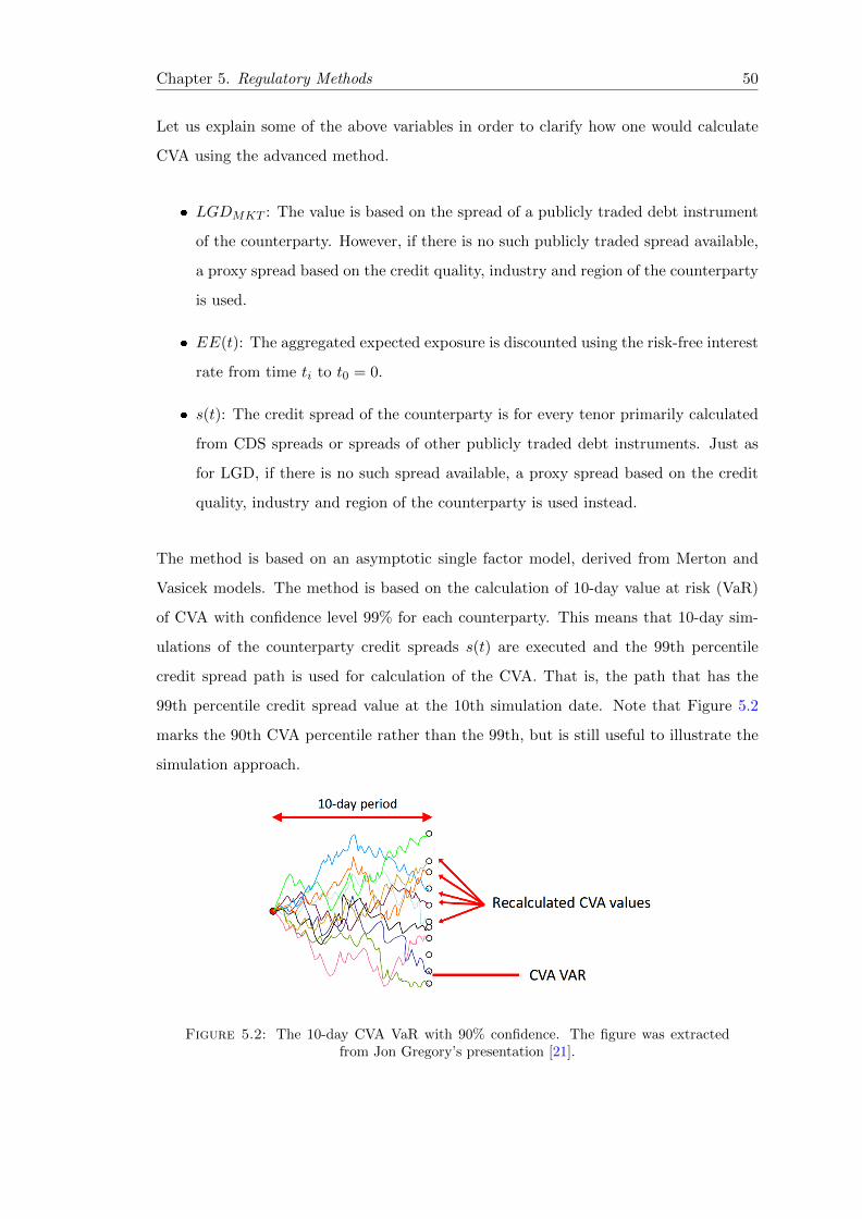
Chapter 5. Regulatory Methods 50
Let us explain some of the above variables in order to clarify how one would calculate
CVA using the advanced method.
� LGDMKT : The value is based on the spread of a publicly traded debt instrument
of the counterparty. However, if there is no such publicly traded spread available,
a proxy spread based on the credit quality, industry and region of the counterparty
is used.
� EE(t): The aggregated expected exposure is discounted using the risk-free interest
rate from time ti to t0 = 0.
� s(t): The credit spread of the counterparty is for every tenor primarily calculated
from CDS spreads or spreads of other publicly traded debt instruments. Just as
for LGD, if there is no such spread available, a proxy spread based on the credit
quality, industry and region of the counterparty is used instead.
The method is based on an asymptotic single factor model, derived from Merton and
Vasicek models. The method is based on the calculation of 10-day value at risk (VaR)
of CVA with confidence level 99% for each counterparty. This means that 10-day sim-
ulations of the counterparty credit spreads s(t) are executed and the 99th percentile
credit spread path is used for calculation of the CVA. That is, the path that has the
99th percentile credit spread value at the 10th simulation date. Note that Figure 5.2
marks the 90th CVA percentile rather than the 99th, but is still useful to illustrate the
simulation approach.
Figure 5.2: The 10-day CVA VaR with 90% confidence. The figure was extractedfrom Jon Gregory’s presentation [21].
Chapter 5. Regulatory Methods 51
Thi calculation of the CVA is performed according to (5.20). Two separate versions of
the computation are carried out. The first calculation is calibrated using market data
from the current one year period. The second is calibrated for a stressed one year period,
with increased credit spreads. The calculations are then added according to (5.21), to
produce the CVA capital charge amount
KadvCV A = 3
[CV Aadvcurrent + CV Aadvstressed
]. (5.21)
The expected exposure in the advanced method is calculated using the internal model
method. This is the reason firms using the advanced approach also need an approval
from regulators on an internal interest rate model.
One slight problem with the advanced model is that is assumes the portfolio to be per-
fectly granular and well diversified internationally. This results in a calculation error
which is hard to estimate accurately. Further, in order to calculate the CVA with the
advanced method, extra data is required in comparison to the methods under the stan-
dardized approach. The financial institutions lacking this data for a sufficient historical
period of time miss out on the opportunity to use the advanced approach for calculating
CVA.
Loss Given Default
It is important to note that LGDM in (5.20) represents the market expectations of the
loss given default. This means that firm specific expectations of recovery must not be
used. The exception is if the seniority of the netting set differs from that which the
markets’ expectations are based on [22].
Merton model
The main models used to simulate the CVA capital charge under the advanced method
are as mentioned before, the Merton and Vasicek models. The Vasicek is somewhat
explained in Section 6.4.1, but we would like to very briefly explain the Merton model
here, for a more complete picture of the advanced method.

Chapter 5. Regulatory Methods 52
The Merton model is one of the most popular methods for simulating the default risk of
a firm. The model defines a firm as defaulted when the firm’s value falls below its debt.
The approach is based on a simulation of market values, market value volatilities and
liability structures, that generate probability of default curves. Two separate processes
are needed for an implementation of the Merton model.
1. One short term interest rate process
2. One process modelling the the total value of a firm’s assets
In the context of the advanced CVA approach, the 1 percent worst PD curve is used
when computing the CVA capital charge.

Chapter 6
CVA calculation for interest rate
swaps
6.1 Calculation methods
The purpose of this chapter is demonstrating how to calculate unilateral regulatory CVA
for a number of distinct interest rate swap portfolios. The computations are executed
using two of the methods described in previous chapters in order to enable a comparison.
Our hopes with the chapter are to be able to conclude under what circumstances a certain
method of calculation may be used and also what method will give the smallest amount
of regulatory capital in general. In the comparison, we will focus on the contribution
from the expected exposure and probability of default factors on CVA. The loss given
default will for simplicity be given a value of 0.6. The reasons behind this number may
seem vague and unscientific, but this according to a survey by Ernest & Young [17], this
seems to be the standard market convention among banks.
All calculations displayed throughout the chapter are executed in Matlab 2013b (8.2.0.701).
Below is an overview of the computations we have performed.
- Internal model method: Firstly, CVA is computed using the IMM. This method
has a moderate support in Matlabs most recent version of the Financial Instru-
ments Toolbox.
- Current exposure method: Secondly, CVA is computed using the simpler CEM.
53

Chapter 6. CVA calculation for interest rate swaps 54
The reason to why we are not using the advanced method as benchmark for regulatory
CVA, is due to the complexity of the model and difficulty in finding the needed data.
The advanced model require the simulation of future default probabilities of included
companies, e.g. using the Merton model. Such models demand data that is hard to
come over, see Section 5.3.1.
6.2 The interest rate swap
In this section a brief explanation of the interest rate swap (IRS) will be given for readers
unfamiliar with financial instruments. Thereafter the market value and mathematical
expression of the CVA of an interest rate swap will be described.
An interest rate swap is an agreement between two parties to exchange a interest rate
cash flows on specified intervals and over a certain period of time. Interest swaps are
OTC derivative contracts, which is one of the reasons to why we will consider them here.
There are a number of different version of IRS contracts, but the far most common type,
and the one we will consider in this chapter, is the so called plain vanilla interest rate
swap. Under this contract, one of the parties pay a fixed interest rate, and the other
pays a floating rate. The convention is that the party paying the fixed rate is called the
payer, and the party receiving the fixed rate is called the receiver. The interest rate is
paid on a so called notional amount (or notional principal amount or notional value);
an imaginary value which is never exchanged.
As the name suggests, the fixed rate of the IRS is decided when signing the swap contract
and does not change during the life of the contract. The floating rate on the other hand
may vary with time, and is most often tied to a reference rate, that sets the floating
rate at every point in time. Common reference rates are the LIBOR-, EURIBOR- and
IOS-rates. In our analysis we used LIBOR rate data to set the parameters for the short
interest rate simulations.
Below is a simple graphical representation of two banks with an interest rate swap
agreement. Bank A receives the fixed rate and is hence called the receiver, while bank B
is the payer. The floating rate paid has EURIBOR as reference rate and an additional
spread usually given in basis points (bps), with 1bp equalling 0.01%.

Chapter 6. CVA calculation for interest rate swaps 55
Figure 6.1: An interest rate swap agreement between bank A and B with the floatingleg tied to the EURIBOR rate.
Let V (t) be the value of the swap at time t, ignoring the counterparty credit risk and
denoting the rate of return by R. Now, if the counterparty defaults at time τ we may
end up in two situations;
if V (τ) ≥ 0 we receive R× V (τ),
if V (τ) ≤ 0 we owe V (τ) to the bankruptcy estate.
We can here see the imbalance in the cash flows depending on if the MtM value is
positive or negative. The payoff can also relatively straightforwardly be expressed in in
a single equation,
P = V (τ)− (1−R)max(V (τ), 0). (6.1)
I the below figure one can see the cash flow asymmetry when a counterparty actually
defaults. In case the MtM values is negative, the entire MtM value is payable to the
bankruptcy estate, while if the MtM is positive, only the rate of return times the MtM
is received. Hence there is a risk associated with both positive and negative MtM
movements.
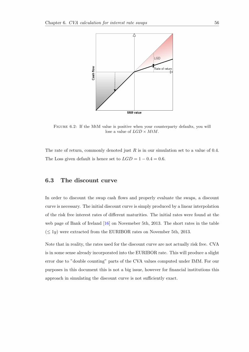
Chapter 6. CVA calculation for interest rate swaps 56
Figure 6.2: If the MtM value is positive when your counterparty defaults, you willlose a value of LGD ×MtM .
The rate of return, commonly denoted just R is in our simulation set to a value of 0.4.
The Loss given default is hence set to LGD = 1− 0.4 = 0.6.
6.3 The discount curve
In order to discount the swap cash flows and properly evaluate the swaps, a discount
curve is necessary. The initial discount curve is simply produced by a linear interpolation
of the risk free interest rates of different maturities. The initial rates were found at the
web page of Bank of Ireland [16] on Novemeber 5th, 2013. The short rates in the table
(≤ 1y) were extracted from the EURIBOR rates on November 5th, 2013.
Note that in reality, the rates used for the discount curve are not actually risk free. CVA
is in some sense already incorporated into the EURIBOR rate. This will produce a slight
error due to ”double counting” parts of the CVA values computed under IMM. For our
purposes in this document this is not a big issue, however for financial institutions this
approach in simulating the discount curve is not sufficiently exact.

Chapter 6. CVA calculation for interest rate swaps 57
Maturity Rate
(months)
3 0.00227
6 0.00341
12 0.00446
24 0.00534
36 0.0071
48 0.0089
60 0.0106
84 0.015
120 0.0199
180 0.0244
240 0.0259
Table 6.1: Initial rates used in the CVA calculation.
Figure 6.3: The initial yield curve at settlement date built from the rates in the abovetable.
6.4 Internal Model Method (IMM)
The following are the settings used in the simulation of the CVA under IMM;

Chapter 6. CVA calculation for interest rate swaps 58
Parameter Value
Settlement date 2013-11-05Principal Amount 1MSEKLatest floating rate 0.00227Rate Spread 10 bpsCash flow frequency once per yearNumber of simulation paths 500Time step 1 monthCompounding continuousIMM α 1.4
Further, the latest floating rate is set equal to the 3-month EURIBOR at 2013-11-05.
The alpha is set to the standard value of 1.4.
It is worth noting that this simulation approach considers the probability of default to
be independent of the exposure and will hence disregard any wrong way risks. Hence,
if there is obvious signs of wrong way risk in the portfolio, this value may suggest a
too small amount of regulatory capital. The consequence of this of course being that
the company having the portfolio may not survive in the long run, as a consequence of
assuming too much counterparty credit risk.
Since the computation considers portfolios of interest rate swaps, the risk factor we face
is the interest rate. In this example we let the floating rate of the swap be indexed
to the 3-month EURIBOR reference rate. The calculation is somewhat complex and is
performed in a number of steps summarized below.
1. Interest rate simulation parameters are obtained from historical EURIBOR market data.
2. The parameters are used to simulate a large number of future interest rate scenarios.
3. Swap prices are computed for every scenario at certain future points in time.
4. Exposures are computed from the prices, taking into account netting and collateral agree-
ments.
5. The exposures are discounted and the average of the values are computed for each simu-
lation date.
6. All the above results are used to compute the regulatory CVA for each counterparty.
The effective maturity for a netting set under the IMM is simple calculated using (5.19).

Chapter 6. CVA calculation for interest rate swaps 59
6.4.1 Interest rate simulations
The interest rate simulation is based on historical data of the three month EURIBOR
rate, from 1999 to the imaginary settlement date 2013-11-05. The needed parameters
are obtained from this data so that a Monte Carlo simulation may be executed. Recall
that the fit of parameters for IMM should be carried out with one normal dataset and
one stressed dataset. This requirement is for simplification not met for our interest
rate simulations. This should anyhow be a big issue, since market rates from the latest
financial crisis is included in the dataset. Below in Figure 6.4 we see the historical 3-
month EURIBOR rate used for the simulation, and additionally the 6- and 12-month
rates.
Figure 6.4: The EURIBOR rate in 2013 is much lower than it has been historically.The dotted line represents the 3M rate data, which is used for the short rate simulations.
The simulations are performed using one of the most used interest rate evolution models,
called the Hull-White single factor (or one-factor) model, which was first described in
the year 1990. The most general definition of a single factor model is
dr(t) = [θ(t)− α(t)r(t)] dt+ σdW (t), (6.2)
where

Chapter 6. CVA calculation for interest rate swaps 60
dr The change in interest rate as a result of a infinitesimal increment of the time dt
α(t) Mean reversion rate
σ Volatility of the rate
dW A Weiner process
θ(t) Drift function
The Hull-White single factor model considers α to be constant in time so that α(t) = α.
There are other one factor model worth noting here. One is the simpler Vasicek model
introduced 1977, which presume that both θ and α are constant. Two other are the
Cox–Ingersoll–Ross (CIR) model from 1985 and the Black–Karasinski introduced in
1991.
Returning to this interest rate simulation, the constants α and σ are extracted from the
historical 3-month EURIBOR rates, using the Matlab function regress. The drift
function θ(t) is defined as
θ(t) = F ′t(0, t) + αF (0, t) +σ2
2α
(1− e−2αt
), (6.3)
withF (0, t) Instantaneous forward rate at time t
F ′t(0, t) Partial derivative of F with respect to t
Equation (6.2) is used to simulate the short (3 month) interest rates. The entire interest
rate curve is thereafter expanded from the short rate using (6.4), which are built in
Matlab functions
R(t, T ) =− 1
(T − t)lnA(t, T ) +
1
(T − t)B(t, T )r(t) (6.4)
lnA(t, T ) = lnP (0, T )
P (0, t)+B(t, T )F (0, t)− 1
4α3σ2(e−αT − e−αt)2(e2αt − 1)
B(t, T ) =1− e−α(T−t)
α.
The matlab functions implementing 6.4 are used in this document without any deeper
analysis, and considered to be outside the narrow scope of this simulation section. After
interpolating the risk free rate between the future times, a discount surface is obtained
for different future observation times and with different tenors. Below are two examples

Chapter 6. CVA calculation for interest rate swaps 61
of yield surfaces obtained in one interest rate simulation. Observe the difference between
the evolution of the short (3 month) rate and how the rate stays non-negative at all times.
Figure 6.5: The simulated yield curve evolution of scenario 15. The short rate keepslow during the five year period.
Figure 6.6: The simulated yield curve evolution of scenario 16. The short rate in-creases noticeably during the five year period.
6.4.2 Exposures
For each scenario the swaps are priced at each future simulation date. At this point, an
approximation is performed, using the Matlab price approximation function, hswapapprox.

Chapter 6. CVA calculation for interest rate swaps 62
(This function estimates the latest floating rate with the 1-year rate. Since the simula-
tion dates do not necessarily correspond to the cash flow dates of the swaps, the 1-year
rate is computed by interpolating linearly between the nearest simulated rates.) The
below figure shows the MtM price evolution of a small portfolio consisting of six 5-year
interest rate swaps. In three swaps we are paying, and in three we are receiving, which
is causing the symmetric appearance.
Figure 6.7: The MtM price evolution of a small portfolio of 5-year interest rate swaps.
The swap prices are saved in a 3 dimensional structure (or matrix) with one simula-
tion date dimension, one instrument dimension and one scenario dimension. From this
structure, the expected exposure terms (EE, EEE, EPE and EEPE - see section 5.2.4)
may easily be obtained by using the discount surface from the interest rate simulations.
Under the IMM, the effective expected positive exposure may thereafter be used to
compute the CVA capital charge.
The CVA capital charge for each netting set may now be calculated by (5.1), using the
effective expected positive exposure (5.18). The total CVA capital charge may thereafter
easily be computed by summing the contributions from each netting set.

Chapter 6. CVA calculation for interest rate swaps 63
6.5 Current Exposure Method (CEM)
Implementing the calculation of the CVA regulatory capital under the CEM is truly
much simpler than that of IMM. Equation (5.9) is used in a straightforward way, and if
netting can be applied, (5.10) is used to compute the netted potential future exposure.
The effective maturity for a netting set under the CEM is simple calculated using (5.12).

Chapter 7
Results and Conclusion
7.1 Stress Tests
In this section we look into some standard cases and a few stress tests for calculating
CVA capital charge using the CEM and IMM, and compare them mutually. We will
stress contracts mainly by changing the counterparty’s rating and time to maturity of
the contracts. We will also analyse and manipulate the credit conversion factor for
maturities greater than 5 years and see what kind of effect that have on the overall
calculation. The credit conversion factor, as mentioned previously, only affect the CVA
capital charge under the CEM.
Note that all the results in this chapter are produced in a setting where the maturities
are slightly (1 day) longer than the integer years stated in the table. As you will see,
this additional one day in time to maturity has a large effect on the results for CEM.
7.1.1 Stress test 1 - Rating drop
In this first section we simulated CVA for 4 different counterparties with different rating
shown in the table below. In all scenarios we are the fixed receiver and the contracts
have the same time-to-maturity of 5 years. We can see the calculated CVA for the
different methods, IMM and CEM in the table below.
64

Chapter 7. Results and Conclusion 65
Counterparty 1 2 3 4
Rating AAA BBB B CCC
Weight×100 0.7 1.0 3.0 10.0
Time to Maturity 5 5 5 5
CV AIMM 60260 86090 258270 860910
CV ACEM 122400 174800 524500 1748500
Difference 62140 88710 266230 887590
Table 7.1: CVA computed for 4 different counterparties with different rating but thesame time-to-maturity, using CEM and IMM method
Figure 7.1: CVA simulated for 4 different contracts with declining credit rating butfixed time-to-maturity
We can here see that CEM is always calculating a higher CVA value than the IMM
method. In this case, the CVA value for the IMM method correspond to approximately
49 % of the CEM value, independent of credit rating. Note though, that the time to
maturity is set to 5 years, which may affect this result. We can however, draw the
conclusion that the CEM-method for calculating CVA is more conservative than the
IMM method.
In this simulation the last time to maturity is slightly over 5 years, in order to get
contribution from the credit conversion factor corresponding to contracts with maturity
over 5 years. The full table of conversion factors can be found in Table 5.2, and the table

Chapter 7. Results and Conclusion 66
showing only the topical interest rate credit conversion factors, can be found below in
Table 7.6.
7.1.2 Stress test 2 - Increasing time to maturity, fixed rating AA
In this portfolio we had 5 contracts with same rating but with increasing time to maturity
from 1 to 5 years. In this test we are the fixed receiver of all contracts. We see that
the CVA value for IMM and CEM coincide until time-to-maturity exceeds 5 years.
The reason why CVA value with CEM method seems to diverge so much from IMM is
because of the conversion factor in the mathematical formulae. The conversion factor is
1.5 for contracts with time-to-maturity greater than 5 years. One can hence analyse the
difference of a portfolio of contracts with time-to-maturity strictly less than 5 years and
see what will happen if you add one extra contract with time-to-maturity greater than
5 years. When looking at the CV AIMM we see a much smoother and more realistic
incline in the change of the capital charge as a function of time to maturity.
Contract 1 2 3 4 5
Rating AA AA AA AA AA
Weight×100 0.7 0.7 0.7 0.7 0.7
Time to Maturity 1 2 3 4 5
CV AIMM 422 4515 12591 29218 60264
CV ACEM 8150 16310 24490 32640 122390
Difference 7728 11795 11899 3422 62126
Table 7.2: CVA simulated for 5 contracts with same credit rating AA and increasingtime-to-maturity, using the CEM and IMM.

Chapter 7. Results and Conclusion 67
Figure 7.2: CVA simulated for 5 contracts with same credit rating AA and increasingtime-to-maturity, using the CEM and IMM.
Contract 1 2 3 4 5
CV AIMM 422 4515 12591 29218 60264
CV ACEM 8150 16310 24490 32640 122390
Fraction 5.2% 27.7% 51.4% 89.5% 49.2%
Table 7.3: Fraction of CVA CV AIMM
CV ACEMfor AA rated contract and 1-5 years to maturity.
When simulating CVA for different time-to-maturities we see that with 1 year to matu-
rity, the CEM method overestimate CVA with 94.8 % compared to the IMM method!
This has to do with the fact that the credit conversion factor at one year to maturity
jumps from 0% to 0.5%. With two years to maturity, the IMM CVA cover 27.7% of
the CEM value. We see that when time-to-maturity is approximately 4 years, the CVA
value of the two methods only differ by approximately 10%. For the last contract with
time-to-maturity greater than 5 years, we see that the CVA value for the CEM method
is approximately twice the value, compared to the IMM method. This last result will
be discussed later.
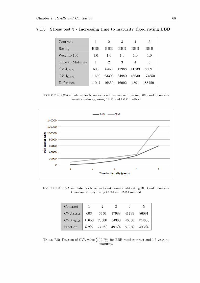
Chapter 7. Results and Conclusion 68
7.1.3 Stress test 3 - Increasing time to maturity, fixed rating BBB
Contract 1 2 3 4 5
Rating BBB BBB BBB BBB BBB
Weight×100 1.0 1.0 1.0 1.0 1.0
Time to Maturity 1 2 3 4 5
CV AIMM 603 6450 17988 41739 86091
CV ACEM 11650 23300 34980 46630 174850
Difference 11047 16850 16992 4891 88759
Table 7.4: CVA simulated for 5 contracts with same credit rating BBB and increasingtime-to-maturity, using CEM and IMM method.
Figure 7.3: CVA simulated for 5 contracts with same credit rating BBB and increasingtime-to-maturity, using CEM and IMM method
Contract 1 2 3 4 5
CV AIMM 603 6450 17988 41739 86091
CV ACEM 11650 23300 34980 46630 174850
Fraction 5.2% 27.7% 48.6% 89.5% 49.2%
Table 7.5: Fraction of CVA value CV AIMM
CV ACEMfor BBB rated contract and 1-5 years to
maturity.

Chapter 7. Results and Conclusion 69
We see that the fraction between CEM method and IMM method is almost exactly the
same as Stress test 2. The only difference is the weight factor due to the BBB rating.
This weight factor of 1.0 scale up the CVA value an equal amount for all maturities in
this test.
7.1.4 Stress test 4 - Manipulation of Credit Conversion Factor
In this section we will try to stress the CVA value in the CEM method by changing
the credit conversion factor. In the standard formula we have credit conversion factor
according to the table below.
Time to Maturity <1yr 1-5 yr 5 yr >
Conversion factor 0 0.5 1.5
Table 7.6: Credit conversion factor for CEM in the standard embodiment
As can be seen in Figure 7.3, the scaling factor of 1.5% for time-to-maturities greater
than 5 years is the reason for the substantial change in slope of the curve under CEM.
Next we will compute CVA using CEM method with a manipulated credit conversion
factor according to the Table 7.7 and analyse the result.
Time to Maturity <1yr 1-5 yr 5 yr >
Conversion factor 0 0.5 0.5
Table 7.7: Credit conversion factor for CEM in the stressed scenario with fixed creditconversion factor

Chapter 7. Results and Conclusion 70
Figure 7.4: CVA capital charge computed using IMM and CEM for BBB-rated coun-terparty, with manipulated credit conversion factor.
As shown earlier in Figure 7.3, we see that the CVA value is always greater when using
the CEM method with normal credit conversion factor. In this figure we can observe a
change in slope for maturities greater than 5 years, which seems to be due to the ccf
value of 1.5%. We have simulated the same contract but stressed the credit conversion
factor for time-to-maturity greater than 5 years to a fixed 0.5%. The output is shown
clear in Figure 7.4. We see that the CVA value for IMM and CEM method intersect
at a point. Without the increase in credit conversion factor for maturities greater than
5 years, the CEM would give a smaller capital charge amount than IMM, which is not
desirable, considering the simplistic computation approach under CEM. One can hence
draw a conclusion that the credit conversion factor is of great importance when it comes
to keeping the CEM more conservative than the IMM.
7.1.5 Comparison of credit rating and maturity stress
This test was performed under the following settings. The base case has one contract
with time to maturity of 4 years and counterparty rating AA. The maturity change is
a change from 4 to 5 years and the rating change is a change from AA to B. This may
seem to be an unrealistic jump in credit rating, but illustrates an interesting point, as
we shall see.

Chapter 7. Results and Conclusion 71
Figure 7.5: CVA capital charge computed using IMM and CEM.
Figure 7.5 shows how the stresses affect the base under IMM and CEM. Comparing the
the CVA capital charges, we may observe that for the base case and rating stress, the
results are fairly similar. For the maturity change, the IMM gives approximately the
double amount of the base case charge, while the CEM gives a result of about four times
the this charge.
Analysing the results for CEM further, we see that increasing maturity of a IRS contract
with one year, gives almost the same change in CVA capital charge as a drop in credit
rating from AA to B. The opinion of the authors is that this is not realistic and that
the IMM agree much more with what one could expect. Especially this is true in the
light of statistics of the cumulative 4-5 year average market sector default probabilities
provided by Fitch, [23]. The document is stating a 0.21% default probability within 4-5
years for AA-rated firms, and 4.04% for B-rated firms. This implying that default of a
B-rated firm is about 20 times more common.
7.1.6 Netting and NGR complications
Performing computations of CVA with netting, we ran into an odd problem. Under
CEM, netting is accounted for via the NGR term, as explained in Section 5.2.2. The

Chapter 7. Results and Conclusion 72
formula is included here once again to facilitate reading;
NGR =max (
∑ni=1MtMi, 0)∑n
i=1 max(MtMi, 0).
Looking at the denominator, we observe that it equals zero if all mark-to-market value
are non-positive. Further, the numerator equals zero if the sum of the mark-to-market
values are less than or equal to zero. For small portfolios this poses a problem, since it
may well happen that all MtM values are negative, meaning that NGR = 0/0. Addi-
tionally, in our examination, this poses a problem, since we are setting the fixed rate so
that MtM of all contracts equal zero at settlement.
The test below was performed to see how the two different methods treat netting of
interest rate swaps. This test was performed using a counterparty with AA-rating and
contracts with just over 5 years to maturity. With the counterparty we have two con-
tracts;
� one in which we are the receivers on a notional amount of 1MSEK,
� and one which we are the payers on a notional stated on x-axis of the figure below
(from 0.2 to 0.8 MSEK).
Hence, there are different degrees of netting possible, depending on the notional amount
of the contract in which we are paying the fixed rate. For example, a reasonable as-
sumption would be that, if the notional amount of contract number two is 0.2MSEK,
then the ”effective” notional amount would be 1− 0.2 = 0.8MSEK.
As explained above, the value of NGR in all these cases is 0/0. Observing from the
formula that both numerator and denominator may not be negative, and that the nu-
merator may equal, but not be larger than the denominator, we conclude that NGR
may only take values in the range [0, 1]. The question now is which of course, which of
these values in this range that makes the most sense. The CVA for both the boundary
values NGR=0 and NGR=1 were therefore plotted.
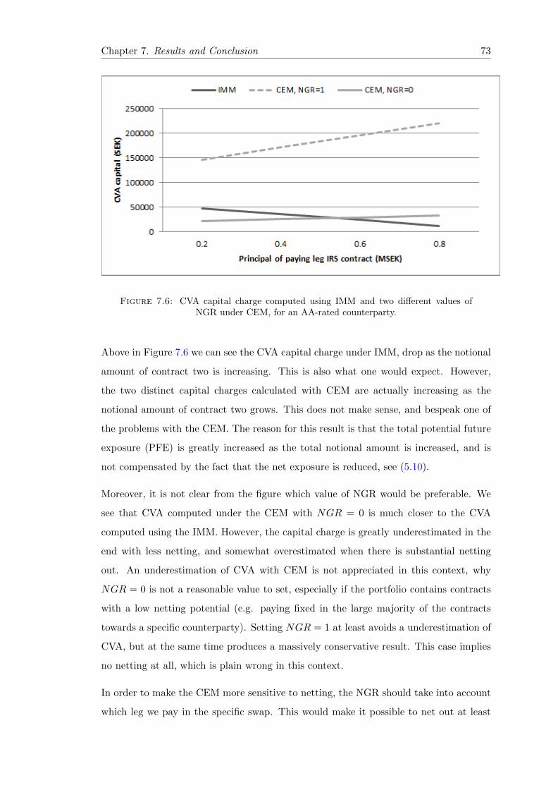
Chapter 7. Results and Conclusion 73
Figure 7.6: CVA capital charge computed using IMM and two different values ofNGR under CEM, for an AA-rated counterparty.
Above in Figure 7.6 we can see the CVA capital charge under IMM, drop as the notional
amount of contract two is increasing. This is also what one would expect. However,
the two distinct capital charges calculated with CEM are actually increasing as the
notional amount of contract two grows. This does not make sense, and bespeak one of
the problems with the CEM. The reason for this result is that the total potential future
exposure (PFE) is greatly increased as the total notional amount is increased, and is
not compensated by the fact that the net exposure is reduced, see (5.10).
Moreover, it is not clear from the figure which value of NGR would be preferable. We
see that CVA computed under the CEM with NGR = 0 is much closer to the CVA
computed using the IMM. However, the capital charge is greatly underestimated in the
end with less netting, and somewhat overestimated when there is substantial netting
out. An underestimation of CVA with CEM is not appreciated in this context, why
NGR = 0 is not a reasonable value to set, especially if the portfolio contains contracts
with a low netting potential (e.g. paying fixed in the large majority of the contracts
towards a specific counterparty). Setting NGR = 1 at least avoids a underestimation of
CVA, but at the same time produces a massively conservative result. This case implies
no netting at all, which is plain wrong in this context.
In order to make the CEM more sensitive to netting, the NGR should take into account
which leg we pay in the specific swap. This would make it possible to net out at least

Chapter 7. Results and Conclusion 74
some of the exposure where one paying and one receiving leg are held against the same
counterparty. Exactly how this would be arranged is outside the intended scope of this
thesis.
7.2 Last words about CEM & IMM
7.2.1 CVA calculation computer intensiveness
We know from derivations of the two methods, IMM and CEM that the IMM method
is much more mathematically sophisticated. The differences in implementation between
the methods imply that the IMM method is much more computer intensive and hence
also requires a lot more time. To analyse and establish this, we used the Matlab com-
mand tic and toc when we simulated CVA for the different portfolios. Under one of the
executions, the CVA capital charge computation time under IMM amounted to 8692 ms,
while the CEM approach required as little as 3.64 ms. The time for reading of input files
is not included in these times. The results obtained are based on a portfolio of only 3
interest rate swaps and using 500 scenario paths under the IMM. In order to get an even
more trustworthy result, one would probably like to increase the number of scenarios to
5000 or so.
Worth noting is that the portfolios that most financial institutions have to calculate
CVA for are massively much larger than the ones used in this document. Hence theses
computations are much more demanding, and in order to obtain more realistic interest
rate scenarios, the use of a shorter time step could prove valuable.
7.2.2 Other aspects of CEM & IMM
So far in this chapter we have seen that from the perspective of the market participants it
seems like getting a IMM approval pays off in terms of regulatory capital. Especially for
firms trading OTC derivatives around the break points of the credit conversion factors
(at maturities slightly longer than 1 and 5 years). Also, the netting benefit achieved
under CEM has some serios flaws and is in some cases almost inexplicable. In fact, firms
operating in the derivatives sector may be forced to get IMM approval in order even to
stay profitable [18]. But there are of course other factors for a firm to consider before

Chapter 7. Results and Conclusion 75
taking the definitive step to IMM approval. One factors is the reputation benefit that
can be achieved by getting the approval.
Also, it is very likely that, in some time the standardized and current exposure methods
will be exchanged for a single non internal model method (NIMM). This is a process
which could potentially take some effort, and instead putting this effort into getting an
IMM approval could be more worthwhile. However, the new non internal model method
could potentially be more risk sensitive than CEM and SM and therefore produce a CVA
capital charge closer to the IMM level. This would of course motivate banks to remain
within the NIMM sphere.
Financial institutions may though consider it wise change to IMM in order to be in line
with the regulatory changes that may, and will, occur in the future. The more complex
and sensitive the utilized model is, the bigger is the chance that it may capture risks
that are not capitalized for today. In this aspect, IMM should clearly be preferential
over CEM. The thing with too simple models is that they risk partially disconnecting
the feel for risk taking from the capital charge amount.
7.2.3 Challenges in obtaining IMM approval
There are obviously some benefit involved in using the internal model method, instead
of the current exposure method. But, what are the main factors to prevent firms from
obtaining an IMM approval? Why are not all firms migrating to the IMM approach for
calculating the CVA capital charge?
Firstly, gaining IMM approval implies making changes to existent processes and models.
The main thing needed is a robust risk engine to perform Monte Carlo simulations,
evaluate a number of different derivative types and compute PFE, EE and CVA.
Additional requirements include systems to identify wrong way risks, and to perform
back-testing and stress testing. The changes will affect processes and models from front
office to credit risk control and reporting systems. Making this kind of changes in an
organization obviously requires a solid understanding of technology and data flows, as
well as approval from senior management. Also, firms need to run the calculations
successfully for 12 months before actually applying it as the regulatory capital charge
Chapter 7. Results and Conclusion 76
calculation [18]. The somewhat short term profit focus in today’s business therefore
counteract the replacement of the CEM for a more sophisticated method.
7.3 Conclusion
The history of counterparty credit risk shows that the CVA measure is here for a reason
and also probably here to stay for a good while. The different methods for computing the
CVA capital charge covers a wide range of method complexities; from the in some senses
over-simplistic current exposure method, to the moderately complex internal model
method, all the way to the advanced model.
This thesis has put forward a few examples of why the IMM is preferable to the CEM.
Therto belong imperfections in the use of credit conversion factors as well as some
abstruse netting behaviours under CEM. However, there fact that all not all firms are
already using the IMM, signifies that the implementation difficulties sometimes outweigh
the benefits.
The bottom line is that CVA provides valuable additional information and understanding
of CCR, which should be taken into account by market participants. How this is done
in practice is up to each distinct participant. Still, the item of greatest importance is
not necessarily how the capital charge is calculated, but merely that the knowledge of
CVA is used and taken into account when managing counterparty credit risk.
7.4 Future work within the topic area
This thesis has indeed only scratched the surface of CVA and its closely related domains.
There is much more that can be done in more or less all areas mentioned. Firstly,
additional stress tests with the current CEM and IMM implementations could easily
be performed to give a more complete picture of how other factors affect the capital
charge under CEM and IMM. A natural expansion would also be to include a more
detailed examination on how collateral and/or central counterparties may reduce the
capital charge.
Chapter 7. Results and Conclusion 77
There are at least two things that could be done to develop the technical aspect of
this document. The most obvious one would be to implement the advanced method in
Matlab to be able to compare all the CVA computation methods in use today. The
second thing would be to update the interest rate model, considering other short rate
models and implement a full interest rate curve simulation engine. The third thing
one could try, is to optimize the credit conversion factors, so that the CVA capital
charge computed under CEM agrees better with the IMM. One approach to escape the
behaviour of the CEM at 1 and 5 years to maturity, would be to fit some suitable smooth
function taking years to maturity as input and returning the credit conversion factor.
A field which remains largely untreated by today’s approach towards CVA is wrong way
risks (WWRs). A more thorough examination of how strongly different kinds of WWRs
may affect the counterparty credit risk would be very highly interesting. Also, a more
detailed analysis of all the XVAs would be desirable. That is, amongst other things,
explaining in more detail how they differ and how they can be properly used in risk
management.

Appendix A
Matlab Code
A.1 main.m
%
% Author: Otto Sjoholm and Dan Franzen
% Created: 2013 -10 -14
% Edited: 2013 -12 -03
%
% Purpose: Main script for calculation of CVA under:
% 1. Internal Model Method (IMM)
% 2. Current Exposure Method (CEM)
%
% Parameters: None
%
% Return: None
%
%dbstop if error
close all
clear all
clc
% Start time measurement
tic
%% Set Constants and read data files
fprintf('\nDefining Constants and reading data files...\n\n')
78

Appendix A. Matlab Code 79
global year numYears horizon scenarioIndex irData swapFile cemFile
dateStr = '2013 -11 -05';
dateFormat = 'yyyy -mm-dd';
dataPath = '.\data\';
irData = strcat(dataPath ,'euribor.xls ');
swapFile = strcat(dataPath ,'swap_portfolio.xls ');
cemFile = strcat(dataPath ,'data_cem.xls ');
[rating , ratingMap] = func_read_rating_data ();
numSwaps = numel(rating.CounterpartyID );
numCounterparties = max(rating.CounterpartyID );
Settle = datenum(dateStr , dateFormat );
RateSpec = func_create_rate_spec( Settle , false );
swapData = func_read_swap_data( RateSpec );
stdCVAimm = struct(...
'Horizon ',[],...
'Weights ',[],...
'Maturities ',[],...
'EAD',[],...
'SinglehPrincipal ',[],...
'SinglehMaturities ',[],...
'IndexhWeights ',[],...
'IndexhPrincipal ',[],...
'IndexhMaturites ' ,[]);
% set time horizon
year = 365;
numYears = 5;
horizon = 1;
scenarioIndex = 200;
% set counterparty data and hedges
w = zeros(numCounterparties ,1);
for i=1: numCounterparties
w(i) = ratingMap(rating.Rating{i ,1});
end
stdCVAimm.Weights = w;
stdCVAimm.SinglehPrincipal = zeros(numCounterparties ,1);
stdCVAimm.SinglehMaturities = zeros(numCounterparties ,1);
% set data for index hedges (here: no hedges are used)
numInd = 1;
stdCVAimm.Horizon = horizon;
stdCVAimm.IndexhWeights = zeros(numInd ,1);

Appendix A. Matlab Code 80
stdCVAimm.IndexhPrincipal = zeros(numInd ,1);
stdCVAimm.IndexhMaturities = zeros(numInd ,1);
stdCVAcem = stdCVAimm;
% display time passed
toc
%% Compute CVA under IMM
fprintf('\nComputing CVA under IMM...\n\n')
numScenarios = 500;
alpha = 1.4;
[EPEcp , EffMaturities] = func_imm_epe(numScenarios , Settle , false );
stdCVAimm.Maturities = EffMaturities;
stdCVAimm.EAD = alpha * EPEcp;
[IMM_CVAcp , IMM_CVAport] = func_compute_cva(stdCVAimm );
% display time passed
toc
%% Compute CVA under CEM
fprintf('\nComputing CVA under CEM...\n\n')
stdCVAcem.Maturities = func_cem_eff_maturity(swapData , Settle );
stdCVAcem.EAD = func_cem_ead(stdCVAcem.Maturities );
[CEM_CVAcp , CEM_CVAport] = func_compute_cva(stdCVAcem );
%% Display Results
fprintf('CVA for each counterparty under IMM (SEK):\n')
disp(IMM_CVAcp)
fprintf('CVA for entire portfolio under IMM (SEK):\n')
disp(IMM_CVAport)
fprintf('Effective maturities for each counterperty under IMM (years ):\n')
disp(stdCVAimm.Maturities)
fprintf('CVA for each counterparty under CEM (SEK):\n')
disp(CEM_CVAcp)
fprintf('CVA for entire portfolio under CEM (SEK):\n')
disp(CEM_CVAport)
fprintf('Effective maturities for each counterperty under CEM (years ):\n')
disp(stdCVAcem.Maturities)

Appendix A. Matlab Code 81
% display time passed
toc
fprintf('\nSimulation Successful !\n')
A.2 func read rating data.m
%
% Author: Otto Sjoholm and Dan Franzen
% Created: 2013 -10 -21
% Edited: 2013 -12 -03
%
% Function: func_read_rating _data.m
%
% Purpose: reads the rating data and rating to weight mapping
% from 'swapFile '
%
% Parameters: None
%
% Return: rating - the rating of each counterparty on the form
% 'AAA ', 'AA ', e.t.c...
% ratingMap - the rating map; mapping every possible rating
% to specific numeric weight
%
% Examples:
%
%
%
function [ rating , ratingMap ] = func_read_rating_data( )
global swapFile
mapData = dataset(...
'XLSFile ', swapFile ,...
'Sheet ', 'RatingMap ');
ratingData = dataset(...
'XLSFile ', swapFile ,...
'Sheet ', 'Rating ');
ratingMap = containers.Map(...
mapData.Rating ,...
mapData.Weight );
rating = struct(...
'CounterpartyID ',[],...

Appendix A. Matlab Code 82
'Rating ' ,[]);
rating.CounterpartyID = ratingData.CounterpartyID;
rating.Rating = ratingData.Rating;
end
A.3 func create rate spec.m
%
% Author: Otto Sjoholm and Dan Franzen
% Created: 2013 -11 -04
% Edited: 2013 -12 -03
%
% Function: func_create_rate_spec.m
%
% Purpose: Creates structures containing information of an interest
% rate term structure.
%
% Parameters: Settle - settlement date of swaps
% display_on - boolean which determines if the historical
% euribor rates should be displayed in a plot
% or not
%
% Return: RateSpec - structure containing properties of an
% interest term structure
% RateCurveObj - interest rate curve represented with data
% Tenor - vector containing the number of months
% where swap rates are specified
%
function [ RateSpec , RateCurveObj , Tenor ] = func_create_rate_spec( Settle , display_on )
global swapFile
zeroCurveData = dataset(...
'XLSFile ',swapFile ,...
'Sheet ','Swap Curve');
Tenor = 12* zeroCurveData.Years + zeroCurveData.Months;
ZeroRates = zeroCurveData.Rate;
ZeroDates = datemnth(Settle , Tenor);
Compounding = -1;

Appendix A. Matlab Code 83
Basis = 0;
RateSpec = intenvset(...
'StartDates ', Settle ,...
'EndDates ', ZeroDates ,...
'Rates', ZeroRates ,...
'Compounding ',Compounding ,...
'Basis ',Basis);
% Create an IRCurve object. We will use this for computing instantaneous
% forward rates during the calculation of the Hull -White short rate path.
RateCurveObj = IRDataCurve(...
'Zero',Settle ,ZeroDates ,ZeroRates ,...
'Compounding ', Compounding ,...
'Basis ', Basis );
if display_on
figure;
plot(ZeroDates , ZeroRates , 'o-');
xlabel('Date');
datetick('keeplimits ');
ylabel('Zero rate'); grid on;
title('Yield Curve at Settle Date');
end
end
A.4 func read swap data.m
%
% Author: Otto Sjoholm and Dan Franzen
% Created: 2013 -10 -21
% Edited: 2013 -12 -03
%
% Function: func_read_swap_data.m
%
% Purpose: reads the swap data from the global variable 'swapFile '
% and uses the RateSpec to set the fixed rate so that the
% swap price is zero at time 0
%
% Parameters: RateSpec - structure containing properties of an
% interest term structure
%
% Return: swaps - structure containing all necessary data to
% price the swap instruments
%

Appendix A. Matlab Code 84
function [ swaps ] = func_read_swap_data( RateSpec )
global swapFile
% Read swaps from spreadsheet
swapData = dataset(...
'XLSFile ',swapFile ,...
'Sheet ','Swap Portfolio Short ');
swaps = struct(...
'Counterparty ',[],...
'NettingID ',[],...
'Principal ',[],...
'Maturity ',[],...
'LegRate ',[],...
'LegType ',[],...
'LatestFloatingRate ',[],...
'FloatingResetDates ' ,[]);
swaps.Counterparty = swapData.CounterpartyID;
swaps.NettingID = swapData.NettingID;
swaps.Principal = swapData.Principal;
swaps.Maturity = datenum(swapData.Maturity , 'yyyy -mm -dd');
swaps.LegType = [swapData.LegType ~swapData.LegType ];
swaps.LegRate = [swapData.LegRateReceiving swapData.LegRatePaying ];
swaps.LatestFloatingRate = swapData.LatestFloatingRate;
swaps.Period = swapData.Period;
swaps.LegReset = ones(size(swaps.LegType ));
%% Set the fixed rate so that the swap price initially is zero
numCounterparties = max(swaps.Counterparty );
for i=1: numCounterparties
LegRate = [NaN swapData.LegRatePaying(i)];
[~, swapData.LegRateReceiving(i)] =...
swapbyzero(...
RateSpec ,...
LegRate ,...
RateSpec.StartDates ,...
swaps.Maturity(i),...
swaps.LegReset(i,:),...
RateSpec.Basis ,...
swaps.Principal(i),...
swaps.LegType(i,:));
end
swaps.LegRate = [swapData.LegRateReceiving swapData.LegRatePaying ];

Appendix A. Matlab Code 85
end
A.5 func imm epe.m
%
% Author: Otto Sjoholm and Dan Franzen
% Date: 2013 -11 -05
%
% Function: func_imm_epe.m
%
% Purpose: Computes the expected positive exposure (EPE) and effective
% maturity under IMM.
%
% Parameters: numScenarios - the number of interest rate scenario
% simulations performed
% Settle - the settlement date of the contracts given
% in MATLAB date number format
% print_on - boolean value indicating if function should
% print status messages when running
%
% Return: EPEcp - effective positive exposure per
% counterparty
% EffMaturity - effective maturity of each netting set
%
function [ EPEcp , EffMaturity ] = func_imm_epe( numScenarios , Settle , print_on )
global irData numYears scenarioIndex
%% Create RateSpec from the Interest Rate Curve
if print_on
fprintf('Creating Rate Curve Object...\n\n')
end
[RateSpec , RateCurveObj , Tenor] = func_create_rate_spec( Settle , false );
%ZeroDates = RateSpec.EndDates;
%% Read Swap Portfolio
if print_on
fprintf('Reading Swap Portfolio...\n\n')
end

Appendix A. Matlab Code 86
swaps = func_read_swap_data(RateSpec );
numSwaps = numel(swaps.Counterparty );
numCounterparties = max(swaps.Counterparty );
%% Set Simulation Parameters
if print_on
fprintf('Setting Simulation Parameter...\n\n')
end
% Compute monthly simulation dates , then quarterly dates later.
simDates = datemnth(Settle ,0:1:(12* numYears ))';
numDates = numel(simDates );
%% Compute Floating Reset Dates
if print_on
fprintf('Computing Floating Rates...\n\n')
end
floatDates = cfdates(Settle -360, swaps.Maturity ,swaps.Period );
swaps.FloatingResetDates = zeros(numSwaps ,numDates );
for i = numDates :-1:1
thisDate = simDates(i);
floatDates(floatDates > thisDate) = 0;
swaps.FloatingResetDates (:,i) = max(floatDates ,[] ,2);
end
%% Read Euribor data
if print_on
fprintf('Reading EURIBOR Data...\n\n')
end
[num ,~,~] = xlsread(irData );
%date_string = txt(2:end ,1);
%date = datenum(date_string ,'yyyy -mm -dd ');
euribor_3m = num(:,3);
%plot(date , euribor_3m );
%datetick('x'), xlabel('Date '), ylabel('Annual Yield (%) ');
%title('3-Month Euribor (Continuously Compounded )');

Appendix A. Matlab Code 87
%% Fit model to data
if print_on
fprintf('Fitting Interest Rate Model Parameters To Data...\n\n')
end
yields = euribor_3m;
regressors = [ones(length(yields) - 1, 1) yields (1:end -1)];
[coefficients , ~, residuals] = regress(diff(yields), regressors );
% The time increment is set depending on the simulation date frequency
dt = mean(diff(simDates ));
% Alpha = Speed: mean -reversion speed
Alpha = -coefficients (2)/dt;
% Level: mean -reversion level
%Level = -coefficients (1)/ coefficients (2);
% Sigma: instantaneous volatility rate
Sigma = nanstd(residuals )/sqrt(dt);
%% Setup Hull -White Single Factor Model
if print_on
fprintf('Setting up Hull -White Single Factor Model...\n\n')
end
r0 = RateCurveObj.getZeroRates(Settle+1,'Compounding ' ,-1);
%r0 = swaps.LatestFloatingRate (1);
t0 = Settle;
% Construct SDE object
FwdRates = RateCurveObj.getForwardRates(...
t0+1:max(swaps.Maturity),...
'Compounding ', -1);
hullwhite1 = hwv(...
Alpha ,...
@(t,x) func_hw_level(t0,t,FwdRates ,Alpha ,Sigma),...
Sigma ,...
'StartState ',r0);
% Store all model calibration information

Appendix A. Matlab Code 88
calibration.RateCurveObj = RateCurveObj;
calibration.Tenor = Tenor;
calibration.ShortRateModel = hullwhite1;
calibration.Alpha = Alpha;
calibration.Sigma = Sigma;
%% Simulate Scenarios
if print_on
fprintf('Simulating Interest Rate Scenarios...\n\n')
end
% Use reproducible random number generator (vary the seed to produce
% different random scenarios).
prevRNG = rng (0);
% Compute interest rate scenarios are their respective discount factors
[scenarios , dfactors] =...
hgenerateScenario(...
calibration ,...
simDates ,...
numScenarios );
% Restore random number generator state
rng(prevRNG );
%% Inspect a Scenario
if print_on
fprintf('Plotting Yield Curve Evolution for Single Scenarios...\n\n')
end
figure;
surf(Tenor , simDates , scenarios (:,:, scenarioIndex ))
axis tight
datetick('y','mmm yy');
xlabel('Tenor (Months)');
ylabel('Observation Date');
zlabel('Rates ');
set(gca ,'View' ,[-49 32]);
title(sprintf('Scenario %d Yield Curve Evolution\n',scenarioIndex ));

Appendix A. Matlab Code 89
%% Compute Mark to Market Swap Prices
if print_on
fprintf('Computing Mark to Market Swap Prices...\n\n')
end
% Compute all mark -to-market values for this scenario. We use an
% approximation function here to improve performance.
values = hcomputeMTMValues(swaps ,simDates ,scenarios ,Tenor );
% The swap value at time t=0 is not simulated , but set to zero.
% The fixed rate set above assures that the price at t=0 equals zero.
values (1,:,:) = 0;
%% Inspect Scenario Prices
if print_on
fprintf('Displaying Single Scenario Prices...\n\n')
end
figure;
plot(simDates , values(:,:, scenarioIndex ));
datetick;
ylabel('Mark -To -Market Price ');
title(sprintf('Swap prices along scenario %d', scenarioIndex ));
%% Visualize Simulated Portfolio Values
if print_on
fprintf('Displaying Portfolio Value in all Scenarios...\n\n')
end
% View portfolio value over time
figure;
totalPortValues = squeeze(sum(values , 2));
plot(simDates ,totalPortValues );
title('Total MTM Portfolio Value for All Scenarios ');
datetick('x','mmm yy')
ylabel('Portfolio Value (SEK)')
xlabel('Simulation Dates')
%% Compute Exposure by Counterparty
if print_on

Appendix A. Matlab Code 90
fprintf('Computing Exposures for each Counterparty...\n\n')
end
instrument_exposures = zeros(size(values ));
unnettedIdx = swaps.NettingID == 0;
instrument_exposures (:,unnettedIdx ,:) = max(values(:,unnettedIdx ,:) ,0);
% We compute exposures per netting agreement , but in this case each
% counterparty has only a single netting agreement.
for i = 1: numCounterparties
nettedIdx = swaps.NettingID == i;
numInst = sum(nettedIdx );
% Exposures for instruments under netting agreements
nettingSetValues = values(:,nettedIdx ,:);
nettedExposure = max(sum(nettingSetValues ,2) ,0);
positiveIdx = repmat(nettedExposure > 0,[1 numInst ]);
% Individual instrument contributions to netting set exposure
instrument_exposures (:,nettedIdx ,:) = nettingSetValues .* positiveIdx;
end
% Sum the instrument exposures for each counterparty
exposures = zeros(numDates ,numCounterparties ,numScenarios );
for i = 1: numCounterparties
cpSwapIdx = swaps.Counterparty == i;
exposures(:,i,:) = sum(instrument_exposures (:,cpSwapIdx ,:) ,2);
end
% View portfolio exposure over time
figure;
totalPortExposure = squeeze(sum(exposures ,2));
plot(simDates ,totalPortExposure );
title('Portfolio Exposure for All Scenarios ');
datetick('x','mmm yy')
ylabel('Exposure (SEK)')
xlabel('Simulation Dates')
%% Exposure Profiles
if print_on
fprintf('Computing All Exposure Types...\n\n')

Appendix A. Matlab Code 91
end
% Expected Exposure
EEcp = mean(exposures ,3);
% Expected Positive Exposure: Weighted average over time of EE
% Here computed using a "trapezoidal" approach
simTimeInterval = yearfrac(Settle , simDates , 1);
simTotalTime = simTimeInterval(end)-simTimeInterval (1);
EPEcp = 0.5*(EEcp (1:end -1 ,:)+ EEcp (2:end ,:))'...
* diff(simTimeInterval )/ simTotalTime;
% EPEport = 0.5*( EEport (1:end -1)+ EEport (2:end))'...
% * diff(simTimeInterval )/ simTotalTime;
%% Compute effective maturity under IMM
EffMaturity = func_imm_eff_maturity( simDates , dfactors , EEcp );
end
A.6 func imm eff maturity.m
%
% Author: Otto Sjoholm and Dan Franzen
% Created: 2013 -10 -28
% Edited: 2013 -12 -03
%
% Function: func_imm_epe.m
%
% Purpose: Computes the effective maturity under IMM
%
% Parameters: simDates - vector of simulation dates on MATLAB serial
% date form
% dFactors - vector of discount factors corresponding to
% the simulation dates
% EE - vectors of expected exposures corresponding to
% the simulation dates
%
% Return: effMaturity - the effective maturity under IMM
%
% Examples:
%

Appendix A. Matlab Code 92
%
%
function [ effMaturity ] = func_imm_eff_maturity( simDates , dFactors , EE)
global year horizon
% Effective Expected Exposure: Max EE up to time simTimeInterval
EEE = zeros(size(EE));
for i = 1:size(EE ,2)
% Compute cumulative maximum
m = EE(1,i);
for j = 1:numel(simDates)
if EE(j,i) > m
m = EE(j,i);
end
EEE(j,i) = m;
end
end
DF = mean(dFactors , 2);
DF = DF(2:end ,:);
EE = EE(2:end ,:);
EEE = EEE (2:end ,:);
dt = diff(simDates) / 365;
limit = simDates (1) + year;
hIndex = find(simDates > limit , 1, 'first ');
Numerator = EE(hIndex:end ,:) '*(DF(hIndex:end ,:).*dt(hIndex:end ,:));
Denominator = EEE(1:hIndex -1,:)'*(DF(1:hIndex -1,:).*dt(1:hIndex -1 ,:));
effMaturity = horizon * (1 + Numerator./Denominator );
end
A.7 func cem ead.m
%
% Author: Otto Sjoholm and Dan Franzen
% Created: 2013 -10 -21
% Edited: 2013 -12 -03
%
% Function: func_cem_ead.m

Appendix A. Matlab Code 93
%
% Purpose: Computes the expected positive exposure (EPE) and effective
% maturity under IMM.
%
% Parameters: Maturities - a vector of the maturities of all swap
% instruments
%
% Return: EAD - the exposure at default for each netting
% set (each counterparty)
%
function [ EAD ] = func_cem_ead( Maturities )
global swapFile cemFile
% Read data from spreadsheets
swapData = dataset(...
'XLSFile ', swapFile ,...
'Sheet ', 'Swap Portfolio ');
cemData = dataset(...
'XLSFile ', cemFile ,...
'Sheet ', 'CCF');
% init structs
swaps = struct(...
'CounterpartyID ',[],...
'Principal ',[],...
'Maturity ' ,[]);
CCF = struct(...
'Maturity ',[],...
'IR',[],...
'FX',[],...
'Equities ',[],...
'Metals ',[],...
'Other ' ,[]);
% fill structs with data
swaps.CounterpartyID= swapData.CounterpartyID;
swaps.Principal = swapData.Principal;
swaps.Maturity = datenum(swapData.Maturity , 'yyyy -mm -dd');
CCF.Maturity = cemData.Maturity;
CCF.IR = cemData.InterestRate;
CCF.FX = cemData.ForeignExchange;
CCF.Equities = cemData.Equities;
CCF.Metals = cemData.Metals;
CCF.Other = cemData.Other;

Appendix A. Matlab Code 94
numSwaps = numel(swaps.CounterpartyID );
numCounterparties = max(swaps.CounterpartyID );
rho = 0.85; % Basel value
CE = 0; % current exposure
Collateral = 0; % collateral
EAD = zeros(numCounterparties ,1);
for i=1: numCounterparties
PFE = [];
MtM = [];
for j=1: numSwaps
if swaps.CounterpartyID(j) == i
%
MtM = [MtM; 0]; % MtM equals 0 at time 0
if Maturities(j) < 1
index = 1;
elseif Maturities(j) < 5
index = 2;
else
index = 3;
end
% potential future exposure (add -on)
PFE = [PFE; swaps.Principal(j)* CCF.IR(index )/100];
end
end
% calculate NGR depending on MtM
if sum(MtM. ^2) == 0
NGR = 1;
elseif sum(max(MtM , 0)) == 0
NGR = 0;
else
NGR = max(sum(MtM), 0) / sum(max(MtM , 0));
end
% compute EAD
Addon = (1-rho + rho*NGR) * sum(PFE);
EAD(i) = CE + Addon - Collateral;
end
end
A.8 func cem eff maturity.m

Appendix A. Matlab Code 95
%
% Author: Otto Sjoholm and Dan Franzen
% Created: 2013 -10 -21
% Edited: 2013 -12 -03
%
% Function: func_cem_eff_maturity.m
%
% Purpose: Computes the effective maturity under CEM for the given
% swap maturities and principals
%
% Parameters: swapData - structure containing the information
% to price all swaps in the portfolio
% Settle - the settlement date for the swaps
%
% Return: eff_maturity - the effective maturity for each netting set
% under CEM
%
function [ eff_maturity ] = func_cem_eff_maturity( swapData , Settle )
global year
contracts = struct(...
'CounterpartyID ',[],...
'Principal ',[],...
'Maturity ' ,[]);
contracts.CounterpartyID = swapData.NettingID;
contracts.Principal = swapData.Principal;
contracts.Maturity = (swapData.Maturity - Settle) / year;
numCounterparties = max(contracts.CounterpartyID );
numContracts = length(contracts.CounterpartyID );
eff_maturity = zeros(numCounterparties ,1);
for i=1: numCounterparties
maturities = [];
principals = [];
for j=1: numContracts
if contracts.CounterpartyID(j) == i
maturities = [maturities; contracts.Maturity(j)];
principals = [principals; contracts.Principal(j)];
end
end
eff_maturity(i) = max(1, (maturities '* principals) / (sum(principals )));
end
end

Appendix A. Matlab Code 96
A.9 func hw level.m
%
% Author: MathWorks
% Created: -
% Edited: -
%
% Function: func_hw_level.m
%
% Purpose: a built in matlab function to compute the mean -reversion
% level of the Hull -White/Vasicek mean -reverting Gaussian
% diffusion model
%
% Parameters: t0 - start time
% dt - time step
% FdwRates - vector of forward rates
% Alpha - mean -reversion speed
% Sigma - instantaneous volatility rate
%
% Return: level - mean reversion level of hwv model
%
function level = func_hw_level(t0 ,dt,FwdRates ,Alpha ,Sigma)
% Compute the level function for the single factor Hull -White short rate
% model.
% Theta function
t = max(t0 + round(dt * 365),t0+1);
theta = Ft(t) + Alpha * F(t) + (Sigma ^2/(2* Alpha)) * (1 - exp(-2* Alpha*dt));
% HW1 level is theta/alpha
level = theta / Alpha / 100;
function r = F(t)
% Instantaneous forward rate
r = FwdRates(t+1-t0);
end
function dr = Ft(t)
% Derivative of the instantaneous forward rate w/ respect to time
Rates = FwdRates(t-t0:t+2-t0);
dr = (Rates (3) - Rates (2)) / (1/365);
end
end

Bibliography
[1] Piterbarg, V. Funding beyond discounting: collateral agreements and derivatives pric-
ing, Risk magazine 97-102, February 2010.
[2] Gielen, F. and Kraev, I. Credit Value Adjustment (CVA): The Standardised Method,
Avantage Reply, November 2011.
[3] KPMG, Basics of Credit Value Adjustments and implications for the assessment of
hedge effectiveness, FinancialCAD, 2011.
[4] IBM Business Analytics, Credit value adjustment - A dynamic approach to pricing
and managing counterparty risk, IBM Corporation, October 2012.
[5] Stampoulis, T. Credit Value Adjustment Trends, Bank of Japan, June 2010.
[6] Fares and Genest, CVA capital charge under Basel III standardized approah, Chap-
puis Halder & CIE, 2012-04-16.
[7] Pykhtin, M. Model foundations of the Basel III standardised CVA charge, Risk mag-
azine, p. 60-66, July 2012.
[8] Non-Cleared OTC Derivatives: Their Importance to the Global Economy, Interna-
tional Swaps and Derivatives Association (ISDA), March 2013.
[9] Alavian, S. et al. Credit Valuation Adjustment (CVA), 2010-10-09.
[10] Gregory, J. The optimization of everything: OTC derivatives, counterparty credit
risk and funding,
https://www.algorithmics.com/think/2012/06/the-optimization-of-everything-otc-derivatives-counterparty-credit-risk-and-funding.
[11] Thompson, T., Dahinden, V. Counterparty Risk and CVA Survey: Current market
practice around counterparty risk regulation, CVA management and funding, Deloitte
and Solum Financial Partners, February 2013.
97

Bibliography 98
[12] Dr. Kotze, A. Current Exposure Method for CCP’s under Basel III, JSE Limited,
May 2012.
[13] Federal Deposit Insurance Corporation, Regulatory Capital Rules: Advanced
Approaches Risk-based Capital Rule; Market Risk Capital Rule, Federal Register,
https://www.federalregister.gov/articles/2013/09/10/2013-20536/
regulatory-capital-rules-regulatory-capital-implementation-of-basel-iii-capital-adequacy-transition,
2013-09-10.
[14] Federal Reserve System, Basel II Capital Accord,
http://www.federalreserve.gov/generalinfo/basel2/draftnpr/npr/
section_5.htm 2013-09-16.
[15] Bank for International Settlements, Amounts outstanding of over-the-counter
(OTC) derivatives by risk category and instrument,
http://www.bis.org/statistics/derstats.htm, 2013-10-08.
[16] Bank of Ireland, Interest Rate Swap Rates, http://corporatebanking.
bankofireland.com/markets/interest-rates/ 2013-11-05.
[17] Ernst & Young, Reflecting credit and funding value adjustments in fair value 2012.
[18] Dr. Williams, A. and Dyson, R. Basel III and gaining IMM approval, Sungard,
2012.
[19] Douglas, R. and Dr. Pugachevsky, D. Comparing Alternate Methods for Calculating
CVA Capital Charges under Basel III Quantifi.
[20] Office of the Superintendent of Financial Institutions Canada, Capital Adequacy
Requirements: Chapter 4 - Settlement and Counterparty Risk, January 2013.
[21] Gregory, J. A Critical Analysis of Counterparty Credit Risk and CVA in a Basel
III World, Solum Financial Partners, November 2012.
[22] Association for Financial Markets in Europe, CRD IV: Credit Valuation Adjustment
(CVA) Advanced CVA formula, 4 May 2012.
[23] Fitch Ratings, Inc., 2013 Form NRSRO Annual Certification https://www.
fitchratings.com/web_content/nrsro/nav/NRSRO_Exhibit-1.pdf 2013-12-10.