credit supply and the price of housing - uzh

Working Paper Series

_______________________________________________________________________________________________________________________

National Centre of Competence in Research Financial Valuation and Risk Management

Working Paper No. 644

Credit Supply and the Price of Housing

Giovanni Favara Jean Imbs

First version: May 2010 Current version: May 2010

This research has been carried out within the NCCR FINRISK project on

“Macro Risk, Systemic Risks and International Finance”

___________________________________________________________________________________________________________

Credit Supply and the Price of Housing�

Giovanni Favara

HEC Lausanne

Swiss Finance Institute

IMF

Jean Imbs

Paris School of Economics

HEC Lausanne

Swiss Finance Institute

CEPR

May 2010

Abstract

We show that since 1994, branching deregulations in the U.S have signi�cantly af-

fected the supply of mortgage credit, and ultimately house prices. With deregulation,

the number and volume of originated mortgage loans increase, while denial rates fall.

But the deregulation has no e¤ect on a placebo sample, formed of independent mort-

gage companies that should not be a¤ected by the regulatory change. This sharpens

the causal interpretation of our results. Deregulation boosts the supply of mortgage

credit, which has signi�cant end e¤ects on house prices. Interestingly, the fraction of

securitized mortgage loans remains unchanged through the process. We �nd evidence

house prices rise with branching deregulation, particularly so in Metropolitan Areas

where construction is inelastic for topographic reasons. We document these results in

a large sample of counties across the U.S. We also focus on a reduced cross-section

formed by counties on each side of a state border, where a regression discontinuity

approach is possible. Our conclusions are strengthened.

JEL Classi�cation Numbers: G21, G10, G12

Keywords: Credit Constraints, Mortgage Market, House Prices, Bank Branching.

�For useful comments, we thank John Driscoll, Tara Rice, Thierry Tressel and participants at seminarsat the IMF, INSEE-CREST, the Federal Reserve board, the MidWest Macroeconomic Meetings 2010, the StLouis Fed, and Universidad Nova de Lisboa. Financial support from the National Center of Competence inResearch �Financial Valuation and Risk Management�is gratefully acknowledged. The National Centers ofCompetence in Research (NCCR) are a research instrument of the Swiss National Science Foundation. Allerrors are our own. Favara: [email protected]; Imbs: [email protected].

1

1 Introduction

Are asset prices a¤ected by the regulation of banks? The answer is key to the modeling

choices that underpin virtually any asset pricing model. And to understanding the response

of �nancial markets to changes in the regulation of �nancial intermediaries, a question of

immediate topical interest. Banking deregulation a¤ects the market structure of credit.

And it can in�uence asset prices either via a demand e¤ect, as more investors participate

in �nancial markets. Or via changes in the discount rate, as liquidity and the risk pro�le

of assets respond to the deregulation. A de�nitive answer is elusive, because of well known

identi�cation issues. The provision of credit is not an exogenous variable. It depends on

asset prices themselves, because some of them can be used as collateral. In this paper, we

identify exogenous shifts to competition in the banking sector, trace their e¤ects on the size

and standards of mortgage loans, and evaluate their end impact on house prices.

Identi�cation rests on regulatory changes to bank branching in the U.S. We focus on post-

1994 interstate branching deregulation. Even though interstate banking was fully legal with

the passage of the Interstate Banking and Branching E¢ ciency Act of 1994 (IBBEA), various

restrictions have remained available for states to hamper interstate branching. For instance,

states are allowed to put limits on banks�size, implementing deposit or age restrictions that

e¤ectively prevent interstate branching. Thus, even after the passage of IBBEA, small and

large banks have continued to struggle for the control of state-level regulation, as Krozner

and Strahan (1999) document they had prior to 1994.

Rice and Strahan (2009) (RS) have constructed an index capturing these e¤ective regu-

latory constraints. They use the index to instrument the conditions of bank credit supply,

and their end e¤ect on �rms��nancing choices. They show restrictions increase with the

proportion of small banks in a state, and decrease with past growth performance. They �nd

no systematic correlation with contemporaneous economic conditions, a result suggestive the

index is abstracting from credit demand. Inasmuch as it focuses on politically driven changes

in credit supply, the index provides a valuable empirical framework to trace the economic

consequences of changes in the availability of credit. In this paper, we merge the deregulation

episodes with county-level information on mortgage loans and house prices. Since the index

runs until 2005, we are able to inform recent developments in the U.S mortgage and housing

markets.

Like RS, Jayaratne and Strahan (1996), or many others, we implement a conventional

treatment e¤ect estimation, where identi�cation obtains across states and over time. We

use this framework to answer three questions: 1) how did branching deregulation impact the

2

mortgage market, 2) did branching deregulation impact house prices, and 3) is the end e¤ect

on house prices channeled via a response of the mortgage market. Detailed information on

the volume and terms of individual mortgage loans has been publicly available since the

Home Mortgage Disclosure Act (HMDA), and we make extensive use of these data. County-

level house price indexes, in turn, are compiled by Moody�s Economy.com. We merge both

data sources with RS index of branching deregulation.

We observe mortgage loans at the county level, which a¤ords a large cross section.

HMDA reports the number, volume, denial rates, securitization and loan-to-income ratios of

mortgage originated both by depository institutions and Independent Mortgage Companies

(IMC). By de�nition, IMC are not a¤ected by bank branching deregulations, and thus not

by the treatment of interest either. They provide a natural placebo sample, which should

not respond to the treatment. The possibility of a di¤erential response across lending in-

stitutions sharpens the causal interpretation of our results. If deregulation were motivated

by an expected increase in the demand for mortgage, it would also correlate signi�cantly

with the volume and conditions of loans originated by IMCs. In fact, our results continue to

obtain when we include directly observable controls for the demand for credit, such as lags

of income or population growth rates, or indeed changes in house prices.

We also observe county-level house price indices. We ask whether their dispersion across

states is signi�cantly related with the chronology of branching deregulation, i.e. whether

an exogenous change in the availability of credit has end e¤ects on the price of housing.

The price of real estate can of course di¤er geographically because of the supply of housing.

Saiz (2009) has compiled information on local topographic characteristics to capture the

amount of developable land in a given area. His measure builds from pre-existing geographic

conditions, and is therefore exogenous to the contemporaneous economic context. We ask

whether the (exogenous) shift in credit supply has a di¤erential e¤ect on the demand for

houses � and ultimately house prices � depending on whether a county is situated in an

area where house construction is particularly inelastic. Such di¤erential response once again

sharpens the causal interpretation of our results.

In the U.S., counties are grouped into Metropolitan Areas (MSA) that sometimes straddle

state borders. These counties provide a focused sub-sample where a regression discontinuity

approach is possible. In such a sub-sample, treated and control counties are neighbors, belong

to the same MSA, and presumably share other unobserved characteristics. The approach

helps put to rest concerns that omitted variable biases plague our estimations. For instance,

local amenities, industrial structure or growth performance can impact simultaneously the

3

mortgage markets, house prices and perhaps the dynamics of deregulation as well. We

begin to address these concerns with county-level �xed e¤ects, and attempts to ascertain

the exogeneity of branching deregulation. A regression discontinuity approach does so in

an exhaustive manner, as any local, unobserved county characteristic is held constant in a

sample of border counties. We implement the approach for both mortgage and house prices

regressions.

We �nd the number and volume of mortgage loans rise with the deregulation episodes,

while denial rates fall. These responses are signi�cant for banks classi�ed as prime lenders,

and larger but not always signi�cant for sub-prime lenders. In addition, the e¤ects we identify

are not channeled via an increase in the fraction of loans that are securitized. Interestingly,

no systematic change is discernible for mortgage loans originated by IMCs. Such di¤erential

e¤ect suggests the shift in credit that we observe cannot be due to demand. If it were, IMCs

would also react and we would observe an universal response of credit. All our conclusions are

sharpened in a sub-sample formed by counties neighboring a state border. Such con�rmation

suggests deregulation, credit, and house prices are not all driven by unobservable variables.

If they were, the relation we document would be weakened in neighboring counties, that

belong to the same metropolitan area.

House prices increase signi�cantly in response to deregulation. The e¤ect prevails hold-

ing constant a battery of conventional controls for changes in the price of housing, including

population and income growth rates. We also allow for an autoregressive component ac-

counting for potential momentum. Interestingly, the response of house prices is non-linear,

as it depends on the constructability at MSA level, captured by Saiz (2009) measure. The

unconditional response of house prices to deregulation is barely signi�cant, but it becomes

strongly positive and signi�cant with a control for the elasticity of housing supply. In MSAs

where constructability is elastic, the e¤ect of branching deregulations is muted. Once again,

the results are sharpened in a sub-sample formed by border counties.

Finally, the end e¤ect of branching deregulations on house prices works via the increase

in the supply of mortgage credit. We regress house prices on the number, volume and denial

rates of mortgage loans, instrumented by the deregulation episodes. The index passes the

conventional tests for weak instruments with �ying colors. The result suggests house prices

respond to a lifting of credit constraints, triggered by an exogenous increase in the supply of

mortgage credit. A shift in credit supply matters for house prices, and branching regulations

a¤ect the access to (mortgage) credit.

Our results that the volume and number of mortgage loans increase with branch dereg-

4

ulation stands in apparent contrast with RS. They �nd price e¤ects but no overall quantity

response. Bank debt rises, but not total borrowing by �rms. RS focus on bank loans con-

tracted by �rms with fewer than 500 employees. They conclude the lack of a response in

overall �rm borrowing underlines the possibly ambiguous impact of competition in the bank-

ing sector, because of adverse selection or the destruction of privileged relationships. Banks

choose to ration credit to �rms, even though borrowing costs have decreased.

In apparent contrast, we �nd positive end e¤ects in the mortgage market. The number

of loans increases and denial rates fall, which suggests a response at the extensive margin.

But we observe mortgage lending on the part of banks, not debtors�overall portfolios. It

is entirely possible overall household debt remains unchanged, as borrowers reallocate their

debt towards mortgage loans. That would mimic exactly what RS �nd for �rms, that resort

increasingly to bank credit in response to the deregulation. No data on the �nancial terms

of mortgages are available, so it is not possible to explore whether the �nancial terms of

mortgage respond to the deregulation in the same way RS document loans to �rms have.

In short, we observe the supply side of the mortgage market (banks), whereas RS observe

the demand side of the credit market (�rms). Our �ndings are not a contradiction with theirs,

as our purpose is di¤erent. We seek to establish whether a regulation induced shift in credit

supply in the mortgage market has consequences on house prices. We remain agnostic as

regards the implications our results have on the e¤ect of banking competition on overall

household debt and bank lending e¢ ciency. They could be identical to what RS conclude.

Our �nding that branching deregulations have an e¤ect on house prices suggests at least

some equilibrium asset prices are a¤ected by the availability of credit. Because of the average

size of the investment relative to available income, and its indivisibility, the purchase of

a house is a top candidate for a transaction that requires access to credit. A house is

the ultimate big ticket item, and its purchase almost always necessitates some borrowing.

Our �ndings are therefore natural, but do not generalize naturally to other assets. They

do however con�rm the �ndings in Mian and Su� (2009a, 2009b) that improved credit

availability facilitates access to house ownership, with end e¤ects on house prices. Mian

and Su� (2009a) stress the role of securitization. The e¤ects we uncover on the mortgage

market do not work via heightened securitization. In fact, the deregulation index provides an

instrument to changes in the mortgage market, and in house prices, that purges out the e¤ects

of securitization. Insofar as RS �nd the index to be exogenous to contemporaneous economic

conditions, it opens the door for sharp causal interpretations. Changes in securitization, in

contrast, potentially depend on (expected) developments on the real estate market.

5

That deregulation should account for a sizeable proportion of the change in the mortgage

market since 1994 in an instrumental variable sense is useful. It suggests bank branch-

ing regulations impose quantitatively important constraints on the availability of mortgage

loans, with end e¤ects on the prices of houses. Branching restrictions, and the ensuing mar-

ket structure in mortgage loans, contribute to explaining in a causal sense the geographic

dispersion in house price dynamics across the U.S.

The rest of the paper is structured as follows. Section 2 introduces our data. In Section

3 we discuss the e¤ect of branching restrictions on the mortgage market, and in Section 4 we

describe the e¤ect on house prices. We also examine both mechanisms jointly in the context

of an instrumental variable estimation. Section 5 concludes.

2 Data

The U.S banking sector has gone through decades of regulatory changes regarding geographic

banking and branching restrictions. In this paper, we focus on branching restrictions. Even

though some states had permitted interstate branching prior to it, it is with the passage of

the IBBEA in 1994 that the formal deregulation of bank branching across state borders was

�nalized. Bank Holding Companies (BHC) could then formally open branches across state

borders without any formal authorization from state authorities. RS argue forcefully states

did still impose rules or limits after 1994, which have de facto hampered interstate branching.

Even though the IBBEA authorized free interstate branching, it also made allowances for

restrictions on the way it can be implemented. RS point to four such restrictions, explicit

in the IBBEA itself. States can restrict (i) the minimum age of the branching bank, (ii)

de novo branching, (iii) the acquisition of individual branches, and (iv) the total amount of

deposits statewide.

According to restriction (i), states can still demand a minimum age for the acquiring

bank � that cannot exceed �ve years. Restriction (ii) stipulates that the opening of new

branches requires explicit agreement by state authorities. Restriction (iii) imposes that

an interstate merger involving several branches rather than the whole target bank must

be agreed explicitly by the state. Finally, the deposit cap allows states to limit the total

amount in insured depository institutions that are controlled by a single bank or BHC. All

four restrictions are likely to a¤ect the intensity of competition in the banking sector, as RS

describe thoroughly. They introduce a time varying index capturing the implementation of

each of the four restrictions across the U.S. states. The index takes values between 0 and 4,

and runs between 1993 and 2005.

6

The Home Mortgage Disclosure Act was passed in 1975 with a view to forcing discrimina-

tion cases out onto the public stage, and to fostering the dissemination of information about

housing investment. Under the Act, any depository institution must report HMDA data if

it has originated or re�nanced a home purchase loan, and if its assets are above an annually

adjusted threshold. Non-depositary institutions, such as Independent Mortgage Companies,

must also report if their house purchase loans portfolio exceeds 10 millions USD. Reporting

depository institutions can be a¢ liates of bank holding companies or subsidiaries of deposi-

tory institutions. They are regulated by the Federal Deposit Insurance Company, the O¢ ce

of the Comptroller of the Currency, the Federal Reserve Board or the O¢ ce of Thrifts Su-

pervision. Independent mortgage companies, instead, are non-depository for-pro�t lenders.

They are supervised at federal level by the Department of Housing and Urban Development.

HMDA data cover information on the borrowing individual (race, ethnicity, income), the

loan�s characteristics (response, reason for denial, amount - but not the interest rate), and

the lending institution.

We aggregate the HMDA dataset up to the county level. We keep track of the number

and volume of loans originated in each county for purchase of single family owner occupied

houses. Loan volume is the total dollar amount aggregated at county level. We compute

a denial ratio, given by the number of loan applications denied divided by the number of

applications received. We also obtain the fraction of originated loans that are securitized.

They are de�ned as loans originated and sold within a year to another �nancial institution

or a government-sponsored housing enterprise. Finally, a loan to income ratio is computed

as the principal dollar amount of originated loan divided by total gross annual applicant

income. Importantly, the numerator is a �ow variable, and captures only imperfectly the

depth of individuals�indebtedness. The �ve variables are computed between 1993 and 2005.

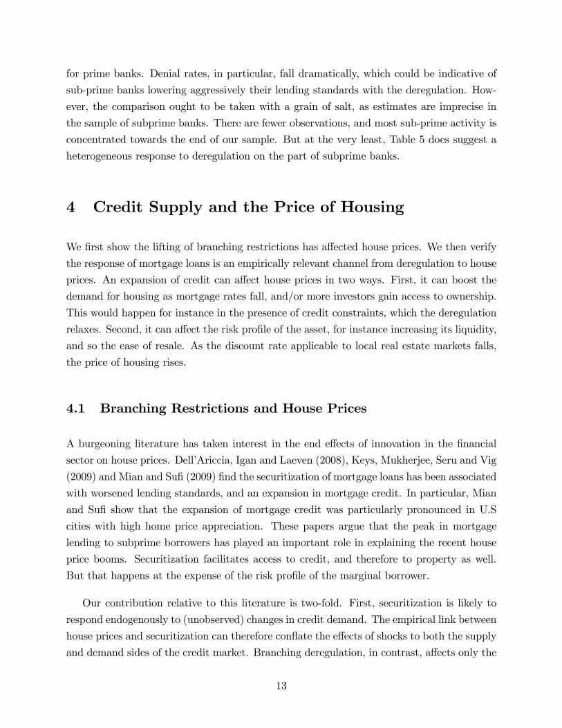
County level house price indexes are collected byMoody�s Economy.com. The series starts

in the 1970�s, and refers to the median house price of existing single family properties. The

series compounds data from a variety of sources, including the US Census Bureau, regional

and national associations of Realtors, and the house prices index from the O¢ ce of Federal

Housing Enterprise Oversight (OFHEO). The sample covers metropolitan counties, where

Moody�s Economy.com index tracks annual changes in house prices. Figure 1 illustrates the

data�s geographic coverage. A prominent alternative would be to use the Case-Shiller index

(CS), which does also provide county-level information. Unfortunately, coverage includes

383 counties only, as against 1,047 for the data we use in the main text. We have veri�ed our

conclusions continue to hold when we implement our estimations on the CS data, in spite of

the heavily reduced sample of counties.

7

Controls for local economic conditions are obtained from the Bureau of Economic Analy-

sis. We collect nominal income per capita and population growth rates at the county level,

between 1993 and 2005. Income per capita is converted in real dollars using the national

Consumer Price Index from the Bureau of Labor Statistics. Finally, we take the index of

house constructability from Saiz (2009). Saiz processed satellite-generated data on water

bodies, land elevation, and slope steepness at the MSA level, to compile an index of land

constructability for all main metropolitan areas in the U.S. The sample is slightly reduced

relative to the rest of our data, but it still covers all metropolitan areas with more than

500,000 inhabitants with available satellite data.

Table 1 lists the variables contained in our dataset, along with their de�nitions and data

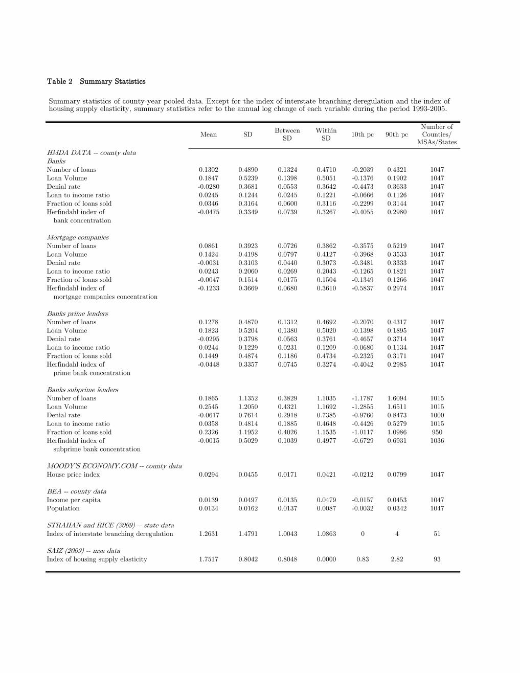
sources. Table 2 reports some summary statistics. We separate out loans characteristics

originated by conventional banks, mortgage companies, and for banks classi�ed as prime or

sub-prime by their regulatory agencies. We have data for 1; 047 counties. For conventional

banks the average annual growth rate in the number of loans is 13%, and the annual average

growth rate in loan value is 18%. The fraction of these loans that are securitized grows at

3:5% per year. Denial rates fall on average by 2:8%, while loan to income ratios rise by

2:4%. During the same period the Her�ndahl index, a measure of market concentration for

mortgage loans, falls by 5%. For each measure, volatility comes mostly from time variation,

rather than dispersion across counties. On the whole, the mortgage market developed less

on average for mortgage companies, with loans numbers and volume expanding less, and

denial rates remaining virtually unchanged. In contrast, the sub-prime mortgage market

expanded faster on average than prime banks, across all four measures we observe. Sub-

prime lenders are not active in all counties, although they are in most. Such average trends

are indicative of di¤erential dynamics across market categories. But of course they are silent

about geographic dispersion since they are merely �rst moments.

House prices increased at an average annual rate of 2:94% between 1994 and 2005, more

than twice faster than average county per capita income. In fact, per capita income and

population grew at virtually identical average rates, around 1:35%. The observed volatility

in house prices comes mostly from time variation, just as loans characteristics did. The same

is true of per capita growth. RS index of branching deregulation is observed at the state

level. On average, the index equals 1:26, so that the average state is relatively restrictive,

with almost three out of four possible restrictions e¤ectively implemented. Dispersion in the

index comes from both state and time variation, which will help identi�cation. Finally, Saiz

index of housing supply elasticity is available for 93 MSAs only, or 485 counties.

8

3 Branching Regulation and Mortgage Credit

Regulations on the geographic expansion of U.S. banks have long been used to characterize

the economic role of �nancial intermediation. Thanks to a history of sequential relaxation

in both banking and branching regulations, U.S states provide a useful laboratory to study

the consequences of changes in the market structure of the banking sector. Jayaratne and

Strahan (1996, 1998), or Stiroh and Strahan (2002) have for instance argued the lifting

of within and between state banking regulations has resulted in observable changes in the

degree of competition amongst banks. With deregulation, banks have improved e¢ ciency,

and lowered non-interest costs. The quality of lending has increased, with lower loan prices,

lower loan losses, and revamping of the overall banks performance. But the regulatory

changes in the banking sector are found to have had little signi�cant impact on the quantity

of credit borrowed by �rms, even though they have observably enhanced competition amongst

banks.

Such a non-result is usually explained by the speci�c consequences of competition in

banking. With less market power, banks �nd it harder to develop privileged relations with

individual borrowers, which acts to worsen issues of asymmetric information (see Petersen

and Rajan, 1995). With more entry, issues of adverse selection become more pressing, so

that banks respond by rationing credit (see Broecker, 1990, Marquez, 2002). The supply of

credit to �rms does not rise, even though competition in the sector has sharpened. Rice and

Strahan (2009) con�rm the conclusion continues to hold for bank lending to �rms, even after

1994, in the most recent period with available data.

We take inspiration from the empirical approach in this literature. We trace the conse-

quences of deregulation in the banking sector on the mortgage market. We depart from most

of the literature in focusing on a speci�c type of bank lending, mostly aimed at households

proposing to acquire real estate property. Identi�cation is conventional and akin to a treat-

ment e¤ect, where deregulated states are treated. Thanks to the established fact branching

deregulation has had mostly political determinants, treatment is exogenous to local economic

conditions (see Kroszner and Strahan, 1999). We estimate

�Lc;t = �1Ds;t + �2�Xc;t + �c + t + "c;t; (1)

where c denotes county-level and s denotes state-level data. �Lc;t is one of the �ve mea-

sures of activity on the mortgage market we observe: growth in the number and volume of

mortgages by county, changes in the denial rate, in the loan to income ratio, and in loan

9

securitization. �Xc;t summarizes county-speci�c controls, which in practice include current

and past growth rates in income per capita, population and house prices, and changes in the

Her�ndahl index of concentration in the mortgage market. Identi�cation rests on the disper-

sion across states (and time) of deregulation, captured by Ds;t. The variable Ds;t aggregates

the four elements of de facto restrictions to interstate branching compiled by RS, and takes

values between 0 and 4.

The controls in �Xc;t help ascertain the e¤ect we identify works through changes in the

supply of mortgage credit. They hold constant conventional determinants of credit demand

at the county level. Following RS, the Her�ndahl index holds constant potential county-

level heterogeneity in the competition on the mortgage market. It brings the focus on the

dispersion across states that is caused by di¤erences in branching restrictions. We focus on

the consequences of deregulation on the growth of the mortgage market, which sets non-

stationarity concerns to rest. We allow for country-speci�c trends in the level of credit via

the inclusion of �c. Our data regroups vastly heterogeneous counties, visually identi�ed

on Figure 1. Such heterogeneity presumably carries through into the underlying dynamics

of the size and characteristics of local mortgage markets. We seek to identify breaks in

these county-speci�c trends, that occur with deregulation. So we estimate growth e¤ects of

deregulation. In addition, t accounts for the overall U.S. credit cycle. Since deregulation

is state-speci�c but loans are observed for each county, standard errors are clustered at the

state level (see Bertrand, Du�o and Mullainathan, 2004).

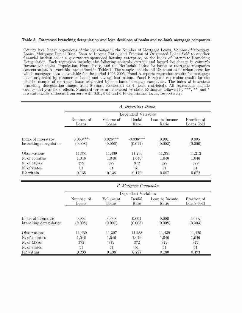
Table 3 presents the results. Panel A focuses on loans originated by depository banks.

The �rst three columns reveal the number of loans and their overall county value both

increase signi�cantly with deregulation, while denial rates fall. All three estimates suggest

the actual size of the mortgage market expands, through a relaxation of the (non-interest)

terms of the loans originated. The point estimate for �1 in the �rst column implies that states

where branching is de facto unfettered experience an annual rate of growth in originated loans

12 percent higher than states that impose full restrictions. The loan to income ratio, however,

does not increase with deregulation. But the measure should be taken with a grain of salt,

since it represents the ratio of debt �ow to income. HMDA does not collect information

on the total level of indebtedness of borrowers. So our measured loan to income ratio may

not correlate signi�cantly with deregulation, even while overall indebtedness increases as a

fraction of income.

The last speci�cation in Table 3 suggests �1 is not di¤erent from zero for the proportion

of originated loans that are resold to other �nancial institutions or government-housing

10

sponsored enterprise, within the year. In other words, the increase in the overall size of

the mortgage market is not accompanied by an increase in securitization. Banks originate

more mortgages, but apparently not with the purpose of contracting credit risk that they

propose to immediately diversify away onto other intermediaries. A shift in the supply

of mortgage credit is observable in response to branching deregulation, but not because

mortgage securitization became rampant at the same time.

A shift in the supply of mortgage loans is entirely compatible with unchanged overall

household debt level. Just as RS found �rms increased bank debt in response to deregula-

tion, but not their overall borrowing, it is possible more households contract a mortgage,

while keeping their overall indebtedness constant. HMDA only reports loans originated: no

information is available about the stock of debt on the demand side. A de�nite con�rmation

of RS�s conclusions on the mortgage market is therefore not an option.

Panel B in Table 3 reports estimates of equation (1) for loans originated by Independent

Mortgage Companies (IMCs). These institutions are una¤ected by changes in branching

regulations, that a¤ect depository institutions only. We �nd deregulation has no e¤ect on

the lending practices of IMCs. In particular, the point estimates of �1 are observably closer

to zero for IMCs than for other lenders, up to an order of magnitude smaller. There is

a di¤erential e¤ect of branching regulations across categories of lenders. This sharpens

the causal interpretation of our estimates. If deregulation were endogenous and simply

responding to expected large increases in the demand for mortgage, �1 should be signi�cant

across both panels in Table 3.

The absence of any signi�cant consequence of deregulation in a placebo sample is also

laying to rest the possibility that �1 is signi�cant because overall economic activity has

accelerated with the deregulation. For instance, Jayaratne and Strahan (1996) show in-

creased e¢ ciency in the banking sector has boosted state-level economic growth. Black and

Strahan (2002) estimate that new business formation has increased following banking re-

form. Morgan, Rime and Strahan (2004) �nd that deregulation has reduced the volatility

of state-level business cycles, as cross-state banking helps insulate each state from shocks to

its own banking system. But such systematic response of the local economy to deregulation

episodes cannot explain a di¤erential response across lenders. The deregulation only a¤ected

mortgage loans originated by a¤ected banks, not the whole mortgage market.

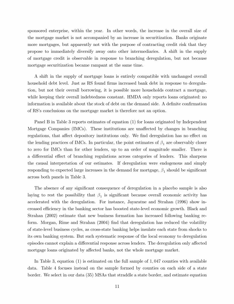
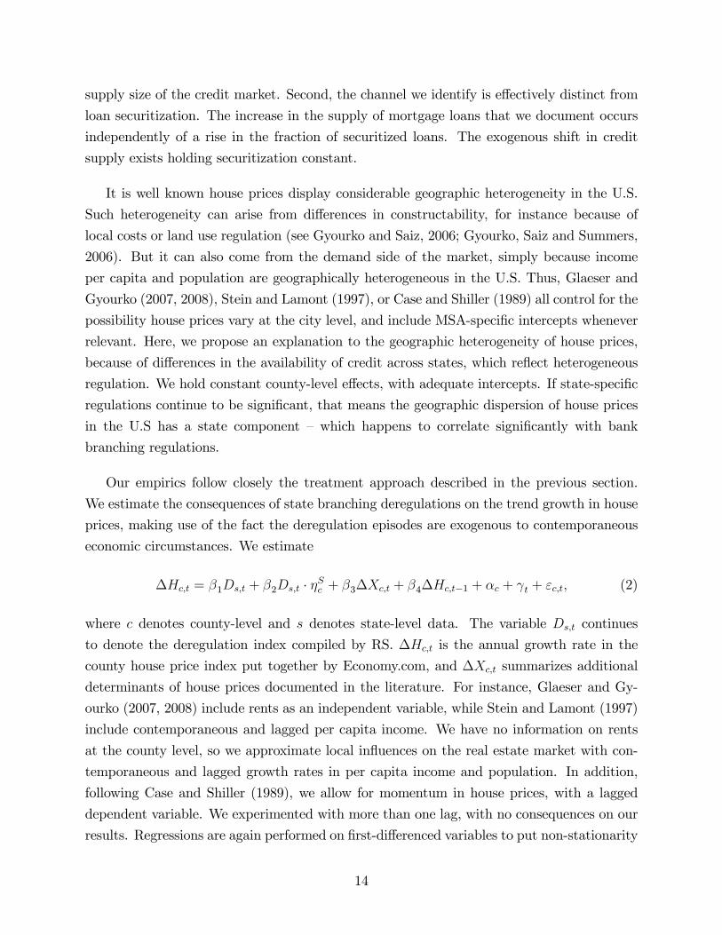
In Table 3, equation (1) is estimated on the full sample of 1; 047 counties with available

data. Table 4 focuses instead on the sample formed by counties on each side of a state

border. We select in our data (35) MSAs that straddle a state border, and estimate equation

11

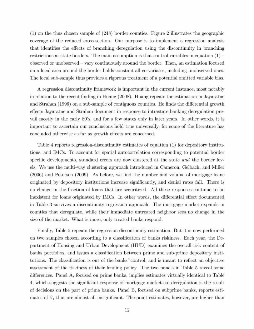
(1) on the thus chosen sample of (248) border counties. Figure 2 illustrates the geographic

coverage of the reduced cross-section. Our purpose is to implement a regression analysis

that identi�es the e¤ects of branching deregulation using the discontinuity in branching

restrictions at state borders. The main assumption is that control variables in equation (1) �

observed or unobserved �vary continuously around the border. Then, an estimation focused

on a local area around the border holds constant all co-variates, including unobserved ones.

The local sub-sample thus provides a rigorous treatment of a potential omitted variable bias.

A regression discontinuity framework is important in the current instance, most notably

in relation to the recent �nding in Huang (2008). Huang repeats the estimation in Jayaratne

and Strahan (1996) on a sub-sample of contiguous counties. He �nds the di¤erential growth

e¤ects Jayaratne and Strahan document in response to intrastate banking deregulation pre-

vail mostly in the early 80�s, and for a few states only in later years. In other words, it is

important to ascertain our conclusions hold true universally, for some of the literature has

concluded otherwise as far as growth e¤ects are concerned.

Table 4 reports regression-discontinuity estimates of equation (1) for depository institu-

tions, and IMCs. To account for spatial autocorrelation corresponding to potential border

speci�c developments, standard errors are now clustered at the state and the border lev-

els. We use the multi-way clustering approach introduced in Cameron, Gelbach, and Miller

(2006) and Petersen (2009). As before, we �nd the number and volume of mortgage loans

originated by depository institutions increase signi�cantly, and denial rates fall. There is

no change in the fraction of loans that are securitized. All these responses continue to be

inexistent for loans originated by IMCs. In other words, the di¤erential e¤ect documented

in Table 3 survives a discontinuity regression approach. The mortgage market expands in

counties that deregulate, while their immediate untreated neighbor sees no change in the

size of the market. What is more, only treated banks respond.

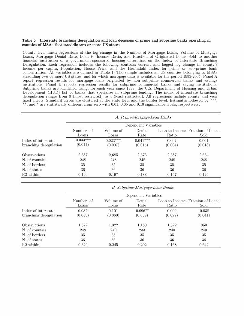
Finally, Table 5 repeats the regression discontinuity estimation. But it is now performed

on two samples chosen according to a classi�cation of banks riskiness. Each year, the De-

partment of Housing and Urban Development (HUD) examines the overall risk content of

banks portfolios, and issues a classi�cation between prime and sub-prime depository insti-

tutions. The classi�cation is out of the banks�control, and is meant to re�ect an objective

assessment of the riskiness of their lending policy. The two panels in Table 5 reveal some

di¤erences. Panel A, focused on prime banks, implies estimates virtually identical to Table

4, which suggests the signi�cant response of mortgage markets to deregulation is the result

of decisions on the part of prime banks. Panel B, focused on subprime banks, reports esti-

mates of �1 that are almost all insigni�cant. The point estimates, however, are higher than

12

for prime banks. Denial rates, in particular, fall dramatically, which could be indicative of

sub-prime banks lowering aggressively their lending standards with the deregulation. How-

ever, the comparison ought to be taken with a grain of salt, as estimates are imprecise in

the sample of subprime banks. There are fewer observations, and most sub-prime activity is

concentrated towards the end of our sample. But at the very least, Table 5 does suggest a

heterogeneous response to deregulation on the part of subprime banks.

4 Credit Supply and the Price of Housing

We �rst show the lifting of branching restrictions has a¤ected house prices. We then verify

the response of mortgage loans is an empirically relevant channel from deregulation to house

prices. An expansion of credit can a¤ect house prices in two ways. First, it can boost the

demand for housing as mortgage rates fall, and/or more investors gain access to ownership.

This would happen for instance in the presence of credit constraints, which the deregulation

relaxes. Second, it can a¤ect the risk pro�le of the asset, for instance increasing its liquidity,

and so the ease of resale. As the discount rate applicable to local real estate markets falls,

the price of housing rises.

4.1 Branching Restrictions and House Prices

A burgeoning literature has taken interest in the end e¤ects of innovation in the �nancial

sector on house prices. Dell�Ariccia, Igan and Laeven (2008), Keys, Mukherjee, Seru and Vig

(2009) and Mian and Su�(2009) �nd the securitization of mortgage loans has been associated

with worsened lending standards, and an expansion in mortgage credit. In particular, Mian

and Su� show that the expansion of mortgage credit was particularly pronounced in U.S

cities with high home price appreciation. These papers argue that the peak in mortgage

lending to subprime borrowers has played an important role in explaining the recent house

price booms. Securitization facilitates access to credit, and therefore to property as well.

But that happens at the expense of the risk pro�le of the marginal borrower.

Our contribution relative to this literature is two-fold. First, securitization is likely to

respond endogenously to (unobserved) changes in credit demand. The empirical link between

house prices and securitization can therefore con�ate the e¤ects of shocks to both the supply

and demand sides of the credit market. Branching deregulation, in contrast, a¤ects only the

13

supply size of the credit market. Second, the channel we identify is e¤ectively distinct from

loan securitization. The increase in the supply of mortgage loans that we document occurs

independently of a rise in the fraction of securitized loans. The exogenous shift in credit

supply exists holding securitization constant.

It is well known house prices display considerable geographic heterogeneity in the U.S.

Such heterogeneity can arise from di¤erences in constructability, for instance because of

local costs or land use regulation (see Gyourko and Saiz, 2006; Gyourko, Saiz and Summers,

2006). But it can also come from the demand side of the market, simply because income

per capita and population are geographically heterogeneous in the U.S. Thus, Glaeser and

Gyourko (2007, 2008), Stein and Lamont (1997), or Case and Shiller (1989) all control for the

possibility house prices vary at the city level, and include MSA-speci�c intercepts whenever

relevant. Here, we propose an explanation to the geographic heterogeneity of house prices,

because of di¤erences in the availability of credit across states, which re�ect heterogeneous

regulation. We hold constant county-level e¤ects, with adequate intercepts. If state-speci�c

regulations continue to be signi�cant, that means the geographic dispersion of house prices

in the U.S has a state component � which happens to correlate signi�cantly with bank

branching regulations.

Our empirics follow closely the treatment approach described in the previous section.

We estimate the consequences of state branching deregulations on the trend growth in house

prices, making use of the fact the deregulation episodes are exogenous to contemporaneous

economic circumstances. We estimate

�Hc;t = �1Ds;t + �2Ds;t � �Sc + �3�Xc;t + �4�Hc;t�1 + �c + t + "c;t; (2)

where c denotes county-level and s denotes state-level data. The variable Ds;t continues

to denote the deregulation index compiled by RS. �Hc;t is the annual growth rate in the

county house price index put together by Economy.com, and �Xc;t summarizes additional

determinants of house prices documented in the literature. For instance, Glaeser and Gy-

ourko (2007, 2008) include rents as an independent variable, while Stein and Lamont (1997)

include contemporaneous and lagged per capita income. We have no information on rents

at the county level, so we approximate local in�uences on the real estate market with con-

temporaneous and lagged growth rates in per capita income and population. In addition,

following Case and Shiller (1989), we allow for momentum in house prices, with a lagged

dependent variable. We experimented with more than one lag, with no consequences on our

results. Regressions are again performed on �rst-di¤erenced variables to put non-stationarity

14

concerns to rest. As before we seek to identify breaks in the trend growth of house prices

that are caused by deregulation, allowing for heterogeneous trends at the county level.1 We

include year e¤ects, which holds constant country-wide cycles in house prices. The focus is

squarely on the state-level dispersion in real estate prices. Standard errors are clustered at

the state level.

The coe¢ cient of interest is �1, that traces the consequences on real estate prices of

deregulation episodes. Even though Ds;t triggers exogenous change in the supply of credit,

the end e¤ect on house prices can re�ect county-speci�c developments on the supply of

houses. Unconditionally positive estimates of �1 can be signi�cant because deregulating

states happen to be ones where house construction is severely restricted. Estimates of �1would be signi�cant, but not because expanding mortgage credit stimulates the demand for

housing. We need to hold constant the supply of houses in equation (2). We do so thanks

to the index of topographic constructability put together by Saiz (2008), which we denote

by �Sc . The variable is e¤ectively observed at the MSA level, so we actually assume the

topography is the same across the counties that form the Metropolitan Areas Saiz considers.

We expect �2 < 0, as house prices should respond less to a credit boom in counties with

plentiful constructable land.

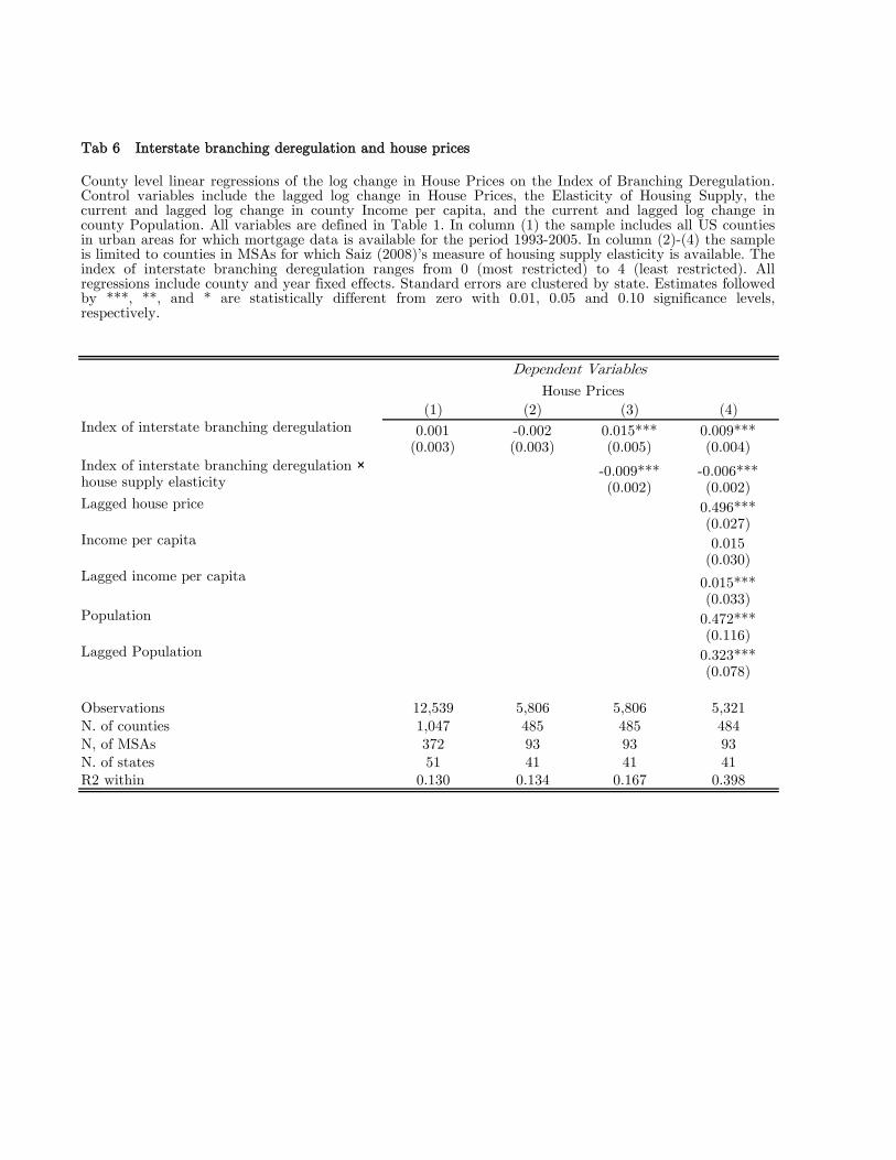
Table 6 presents our estimates of equation (2) for di¤erent control sets. Unconditional

estimates of �1 are insigni�cant, whether they are obtained from the total sample of counties

with house price information (column 1), or we constrain the sample to counties where �Scis available (column 2). Interestingly, �1 becomes positively signi�cant when we control for

the elasticity of house supply �Sc . The interaction term, in turn, is signi�cant and negative,

with �2 < 0 in all instances. These conclusions continue to prevail no matter the control

set across the speci�cations in Table 6. It is only in counties with a topography that makes

house construction di¢ cult that deregulations a¤ect house prices signi�cantly. Their e¤ect

is muted elsewhere.

Controls for population and income growth do not alter the impact of deregulation on

house prices. It is di¢ cult to think of shocks to the demand for credit that do not correlate

with per capita income or population growth, but do correlate with Ds;t. Especially given

the evidence in the previous section that deregulation only a¤ects treated banks in treated

states.1The vast majority of papers using disaggregated house price indexes refrain from using the information

contained in the level of indexes. For instance, Himmelberg, Mayer and Sinai (2005) recommend to focusexclusively on the growth rates in house prices as implied by OFHEO indexes. Units are often not directlycomparable and the cross-section can be a¤ected by the statistical methodology used in computed indexes.We follow the standard and estimate equation (2) in growth rates.

15

The results in Huang (2008) help assuage further such a concern for an omitted variable

bias. Using counties bordering a state frontier, Huang concludes there are relatively few

instances where banking deregulations have had di¤erential growth e¤ects. This is especially

true of the most recent period. In other words, the border discontinuity in per capita income

growth rates is minimal in the recent time period. Income per capita growth rates are on

the whole not a¤ected by the border, and therefore not by the most recent deregulation

chronology either. Observed or unobserved controls in equation (2) thus presumably vary

continuously around state borders. A regression discontinuity estimation will help account for

potential omitted controls. Table 7 presents the results. Interestingly, all coe¢ cients become

larger in magnitude, with unconditionally positive and signi�cant estimates of �1. When an

interaction term involving �Sc is included, estimates for �1 roughly double in magnitude, and

continue to be signi�cantly positive. Estimates of �2, in turn, continue to be negative and

signi�cant.2

These results suggest the relaxation of branching regulations has a causal impact on

house prices at the county level. The end e¤ect depends on the elasticity of housing supply.

We classify a county as �highly elastic� if it falls in the top 10% MSAs according to �Sc ,

and �highly inelastic� if it falls in the bottom 10%: On the basis of column 4 in Table 7,

house prices do not react in highly elastic counties. But in highly inelastic counties, the

lifting of branching restrictions increases the growth rate of house prices by 5 percent per

year. This is a large number, considering the mean growth in real house prices over the

1994-2005 period is 3%.3 A natural interpretation of such estimates is that bank branching

deregulations a¤ect the supply of mortgage credit, and either shift the demand for houses

upwards, or modify their risk pro�le or liquidity. The next section investigates rigorously

the empirical validity of this channel.

4.2 The Credit Channel

In Section 3 we document a signi�cant e¤ect of branching deregulations on the supply of

mortgage loans. We show the response only exists amongst treated banks located in treated

2Equation (2) su¤ers from a conventional bias due to the presence of lagged dependent variables in a�xed e¤ects regression. Blundell and Bond (2000) show the implied bias is bounded below by the coe¢ cientestimates arising from a simple Ordinary Least Squares (OLS) estimator. We estimated equation (2) without�c intercepts, with OLS, and con�rmed all our results, with minimal changes in coe¢ cient estimates. Weconclude the bias is negligible in our dataset and speci�cation.

3We have veri�ed our results are identical in the alternative dataset on county house prices collected byCase-Shiller. The coverage is substantially smaller with only 350 counties, out of which 57 are straddling astate border. In Appendix Tables A1 and A2 we show the end estimates of �1 and �2 are virtually identical.

16

states. This rules out explanations based on an endogenous demand for deregulation, which

would have to arise from both mortgage companies and treated banks located in the same

county. In Section 4, we document the very same deregulation episodes result in rising

house prices. We show the price response prevails mostly in treated counties where the

constructability of houses is physically limited, and continues to exist between neighboring

counties on either side of a state border. In both Sections, we stress a causal mechanism

going from deregulation to the supply of mortgage credit, and from deregulation to the

demand for housing.

We now investigate whether the expansion in credit triggered by deregulation is a quan-

titatively relevant reason for the response of house prices. We do so combining the intuitions

from equations (1) and (2). In particular, we perform an instrumental variable (IV) estima-

tion of

�Hc;t = �1�Lc;t + �2�Xc;t + �3�Hc;t�1 + �c + t + "c;t; (3)

where �Lc;t is instrumented by the deregulation episodes, i.e.

�Lc;t = �1Ds;t + �2�Xc;t + �3�Hc;t�1 + �c + t + "c;t; (4)

The notation is unchanged. Equation (3) continues to include conventional controls for house

price dynamics. We perform the IV estimation on the reduced sample of border counties.

The system formed by equations (3) and (4) investigates econometrically the relevance of

branching deregulations to account for the cross-section in �Lc;t, and ultimately in house

prices.

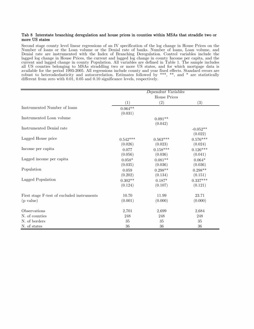
Table 8 presents regression discontinuity results for three measures of �Lc;t, the num-

ber of loans, their volume and the denial rate. The F-test for weak instruments evaluates

the null hypothesis that the instruments Ds;t are excludable from the �rst stage regression

(4). Staiger and Watson (1997) recommend the F-test should take values above 10, lest the

end estimates become unreliable. Branching deregulations satisfy the recommendation in all

three speci�cations in Table 8. The explanatory power of branching deregulations is satis-

factory in an instrumental sense: the dispersion in county-level conditions of the mortgage

market is well explained by Ds;t.

Estimates of �1 are always signi�cant in Table 8. Growing volume and number of loans,

once instrumented by Ds;t, result in rising house prices. And low denial rates, instrumented

by Ds;t, also a¤ect house prices in a causal sense. Thus, the deregulation-induced fraction

of �Lc;t a¤ect the price of houses signi�cantly. Interestingly, a sample focused on subprime

17

banks implies fundamentally di¤erent conclusions. In unreported results, we estimate the

system of equations (3)-(4) on sub-prime banks only. The instrument set never passes the

Staiger-Watson test, with F-test close to zero, and �1 is insigni�cant.

All in all, we have evidence a credit boom on the prime mortgage market is caused

by branching deregulations. There is no such response in the credit supplied by subprime

banks. Such improved access to credit markets causes an increase of house prices, in a

quantitatively signi�cant manner. We conclude the pricing of housing is a¤ected by banking

regulations, via their e¤ects on the mortgage markets. The coe¢ cient estimates in Table

8 point to substantial end e¤ects of deregulation on trend annual growth in house prices,

around 0:5� 1 percentage point increase across the three speci�cations.4 These are impacte¤ects, that are transitory since lagged house prices are signi�cant and �3 < 1 in equation

(3).

5 Conclusion

The price of housing is in�uenced by access to credit, and ultimately by the regulation of

�nancial intermediaries. We establish this claim in a causal sense thanks to an index of

bank branching deregulation compiled by Rice and Strahan (2009). We show deregulation

increases the number, volume and acceptance rates of mortgage origination. More loans are

contracted, but not subsequently securitized. Nor indeed are sub-prime banks clearly more

active. Importantly, only treated banks in treated counties respond to deregulation, which

rules out explanations for our results based on unobserved shifts in the demand for credit.

What is more, such di¤erential e¤ects are sharpened in a regression discontinuity estimation.

House prices rise in deregulated counties, and this response is particularly pronounced

in counties where the supply of housing is inelastic. This holds true across all U.S counties

with house price data, but also for counties neighboring state borders. There, unobserved

determinants for house prices presumably change continuously with distance from the border,

and the focus is squarely on the consequences of bank deregulation on house prices. The

channel that goes from deregulation to house prices works via the response of mortgage

credit supply. It is because the lifting of branching restrictions relaxes the conditions for

mortgage origination that the price of housing increases.

4All variables are measured in logarithms.

18

References

Bertrand, M., E. Du�o and S., Mullainathan (2004). �HowMuch Should we Trust Di¤erence-

in-Di¤erence Estimators?�Quarterly Journal of Economics 119, 1: 249-75.

Black, S. and P. E. Strahan, (2002), �Entrepreneurship and Bank Credit Availability,�Jour-

nal of Finance 57(6), 2807-2833.

Blundell, R. and S. Bond, (2000), �GMM Estimation with Persistent Panel Data: An Ap-

plication to Production Functions,�Econometric Reviews 19(3), 32 1-340.

Broecker, T. (1990), �Credit-Worthiness Tests and Interbank Competition,�Econometrica

58, 429-452.

Cameron, C., J., Gelbach and D., Miller (2006), �Robust Inference with Multi-Way Cluster-

ing.�NBER Technical Working Paper 327.

Case, K. E., and R. J. Shiller (1989), �The E¢ ciency of the Market for Single Family Homes,�

American Economic Review, 79(1), 125-137.

Dell�Ariccia, G., D. Igan, L. Laeven (2008). �Credit Booms and Lending Standards: Evi-

dence from the Subprime Mortgage Market�. IMF Working Paper

Glaeser, E. and J. Gyourko (2006). �Housing Cycles.�NBER working paper 12787

Glaeser, E. and J. Gyourko (2007), �Arbitrage in Housing Markets,�NBER W.P. 13704

Gyourko, J. and A. Saiz (2006). �Construction Costs and the Supply of Housing Structure.�

Journal of Regional Science, vol. 46, No. 4, pp. 661-680.

Gyourko, J., A. Saiz and A.A. Summers (2008). �A New Measure of the Local Regulatory

Environment for Housing Markets: The Wharton Residential Land Use Regulatory Index.�

Urban Studies, vol. 45, No. 3, pp. 693-729.

Himmelberg, C; C Mayer; and T Sinai (2005). �Assessing High House Prices: Bubbles, Fun-

damentals, and Misperceptions.�Journal of Economic Perspectives, vol. 19, number 4 (Fall),

pp. 67-92.Huang R. R. (2008) "Evaluating the real e¤ect of bank branching deregulation:

Comparing contiguous counties across US state borders," Journal of Financial Economics,

87, 678�705

Keys, B., T. Mukherjee, A. Seru, and V. Vig, (2010), �Did Securitization Lead to Lax

Screening: Evidence from Subprime Loans,�Quarterly Journal of Economics, 125

19

Kiyotaki, N� and J. Moore, (1997). �Credit Cycles�, Journal of Political Economy, 105,

211-248.

Kroszner, R.S. and P.E. Strahan (1999). �What Drives Deregulation? Economics and Pol-

itics of the Relaxation of Bank Branching Restrictions.�Quarterly Journal of Economics,

114:1437-67.

Jayaratne, J. and P. E. Strahan (1996), �The Finance-Growth Nexus�, Quarterly Journal of

Economics, 111: 639-670.

Jayaratne, J. and P. E. Strahan (1998), �Entry Restrictions, Industry Evolution, and Dy-

namic E¢ ciency: Evidence from Commercial Banking�, Journal of Law and Economics, 41,

239-273.

Lamont, O. and J. Stein (1997) �Leverage and house-price dynamics in U.S. cities,�Rand

Journal of Economics, 29, 498�514.

Marquez, R., (2002), �Competition, Adverse Selection and Information Dispersion in the

Banking Industry,�Review of Financial Studies 15, 901-926.

Mian, A. R. and Su�, A., (2009a), �The Consequences of Mortgage Credit Expansion: Evi-

dence from the U.S. Mortgage Default Crisis�, Quarterly Journal of Economics 124:

Mian, A. R. and Su�, A., (2009b), �House Prices, Home Equity-Based Borrowing, and the

U.S. Household Leverage Crisis�, Working Paper, Chicago Booth.

Morgan, D. P., B. Rime and P. E., Strahan. (2004), �Bank Integration and State Business

Cycles,�Quarterly Journal of Economics, 119 (4), 1555-1584

Ortalo-Magné, F. and S. Rady (2006), �Housing Market Dynamics, on the Contributions of

Income Shocks and Credit Constraints,�Review of Economic Studies, 73, 459-485.

Petersen, M., (2009), �Estimating Standard Errors in Finance Panel Data Sets: Comparing

Approaches,�Review of Financial Studies, 22, 435-480.

Petersen, M., and R. Rajan, (1994), �The Bene�ts of Firm-Creditor Relationships: Evidence

from Small-Business Data,�Journal of Finance 49: 3-37.

Rice, T., and P.E. Strahan, (2009), �Does Credit Competition a¤ect Small-Firm Finance?,�

forthcoming Journal of Finance.

Saiz, A., (2008), �On Local Housing Supply Elasticity�, Wharton Working Paper, 2008.

20

Staiger, D., and J., Stock, (1997), �Instrumental variables regression with weak instruments,�

Econometrica 65 (3), 557�586.

Stein, J. (1995), �Price and Trading Volume in the Housing Market: A Model with Down-

Payment E¤ects,�Quarterly Journal of Economics, 110, 379-406.

Stiroh, K. J., and P. E. Strahan (2003), �Competitive Dynamics of Deregulation: Evidence

from U.S Banking�, Journal of Money, Credit, and Banking, 35 (5): 801-828.

21

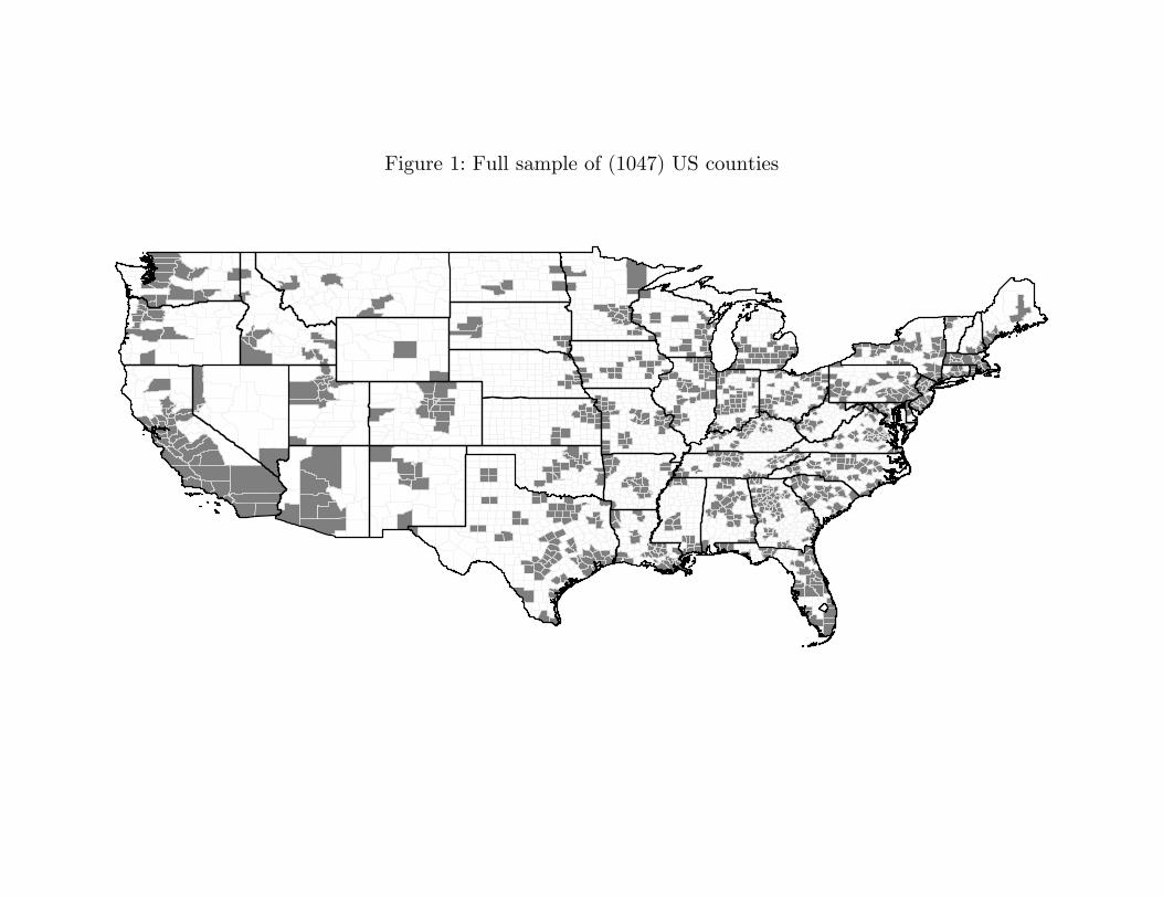
Figure 1: Full sample of (1047) US counties

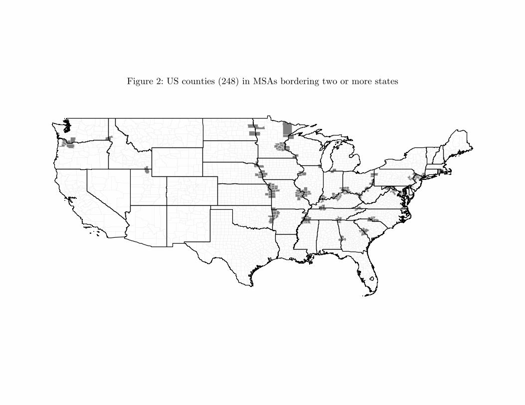
Figure 2: US counties (248) in MSAs bordering two or more states

Ecomony Moody's.com

Saiz (2008)

BEA

BEA

Table 1. Description of Variables and Data Sources

County income per capita

Variable name Variable description Source

County population (in thousands)

Land-topology based measure of housing supply elasticity.

County median price of existing single-family homes.

Index of US interstate branching deregulation based on no limitsto: (1) de novo interstate branching, (2) acquisition of individualbranches, (3) statewide deposit cap and, (4) minimum age of thetarget institution. The index ranges from zero (most restrictive)to four (less restrictive). The index is set to zero in 1993, theyear before the passage of the 1994 Interstate Banking andBranching Efficiency Act (IBBEA).

Index of interstate branching deregulation

Number of loans HMDA

HMDA

HMDA

HMDA

Loan volume

Denial rate

Loan to income ratio

House price index

Housing supply elasticity

Income per capita

Population

Rice and Strahan (2009)

Principal amount of loan originated (in thousands of dollars) forpurchase of single family owner occupied houses divided by totalgross annual applicant income (in thousands of dollars). Countylevel aggregation of loan level data.

Number of loan applications denied divided by the number ofapplications received. County level aggregation of loan level data.

Number of loans originated for purchase of single family owneroccupied houses. County level aggregation of loan level data.

Fraction of loans sold Fraction of loans originated for purchase of single family owneroccupied houses sold within the year of origination to anotherfinancial institution or a government-sponsored housingenterprises. County level aggregation of loan level data.

HMDA

Herfindahl Index Sum of squared shares of mortgage loans. The shares are basedon the number of loans originated by a lender relative to thetotal number of mortgage loans originated in a county. Loans arefor purchase of single family owner occupied houses.

HMDA

Dollar amount (in thousands of dollars) of loans originated forpurchase of single family owner occupied houses. County levelaggregation of loan level data.

HMDA DATA -- county dataBanksNumber of loans 0.1302 0.4890 0.1324 0.4710 -0.2039 0.4321 1047Loan Volume 0.1847 0.5239 0.1398 0.5051 -0.1376 0.1902 1047Denial rate -0.0280 0.3681 0.0553 0.3642 -0.4473 0.3633 1047Loan to income ratio 0.0245 0.1244 0.0245 0.1221 -0.0666 0.1126 1047Fraction of loans sold 0.0346 0.3164 0.0600 0.3116 -0.2299 0.3144 1047Herfindahl index of -0.0475 0.3349 0.0739 0.3267 -0.4055 0.2980 1047 bank concentration

Mortgage companiesNumber of loans 0.0861 0.3923 0.0726 0.3862 -0.3575 0.5219 1047Loan Volume 0.1424 0.4198 0.0797 0.4127 -0.3968 0.3533 1047Denial rate -0.0031 0.3103 0.0440 0.3073 -0.3481 0.3333 1047Loan to income ratio 0.0243 0.2060 0.0269 0.2043 -0.1265 0.1821 1047Fraction of loans sold -0.0047 0.1514 0.0175 0.1504 -0.1349 0.1266 1047Herfindahl index of -0.1233 0.3669 0.0680 0.3610 -0.5837 0.2974 1047 mortgage companies concentration

Banks prime lendersNumber of loans 0.1278 0.4870 0.1312 0.4692 -0.2070 0.4317 1047Loan Volume 0.1823 0.5204 0.1380 0.5020 -0.1398 0.1895 1047Denial rate -0.0295 0.3798 0.0563 0.3761 -0.4657 0.3714 1047Loan to income ratio 0.0244 0.1229 0.0231 0.1209 -0.0680 0.1134 1047Fraction of loans sold 0.1449 0.4874 0.1186 0.4734 -0.2325 0.3171 1047Herfindahl index of -0.0448 0.3357 0.0745 0.3274 -0.4042 0.2985 1047 prime bank concentration

Banks subprime lendersNumber of loans 0.1865 1.1352 0.3829 1.1035 -1.1787 1.6094 1015Loan Volume 0.2545 1.2050 0.4321 1.1692 -1.2855 1.6511 1015Denial rate -0.0617 0.7614 0.2918 0.7385 -0.9760 0.8473 1000Loan to income ratio 0.0358 0.4814 0.1885 0.4648 -0.4426 0.5279 1015Fraction of loans sold 0.2326 1.1952 0.4026 1.1535 -1.0117 1.0986 950Herfindahl index of -0.0015 0.5029 0.1039 0.4977 -0.6729 0.6931 1036 subprime bank concentration

MOODY'S ECONOMY.COM -- county dataHouse price index 0.0294 0.0455 0.0171 0.0421 -0.0212 0.0799 1047

BEA -- county dataIncome per capita 0.0139 0.0497 0.0135 0.0479 -0.0157 0.0453 1047Population 0.0134 0.0162 0.0137 0.0087 -0.0032 0.0342 1047

STRAHAN and RICE (2009) -- state dataIndex of interstate branching deregulation 1.2631 1.4791 1.0043 1.0863 0 4 51

SAIZ (2009) -- msa dataIndex of housing supply elasticity 1.7517 0.8042 0.8048 0.0000 0.83 2.82 93

Table 2 Summary Statistics

Mean SD 10th pc 90th pcNumber of Counties/

MSAs/States

Between SD

Within SD

Summary statistics of county-year pooled data. Except for the index of interstate branching deregulation and the index of housing supply elasticity, summary statistics refer to the annual log change of each variable during the period 1993-2005.


0.030*** (0.008)

0.026*** (0.006)

-0.036*** (0.011)

0.001 (0.002)

0.005 (0.006)

Observations 11,351 11,439 11,293 11,351 11,212N. of counties 1,046 1,046 1,046 1,046 1,046N. of MSAs 372 372 372 372 372N. of states 51 51 51 51 51R2 within 0.135 0.138 0.179 0.087 0.072


0.004 (0.008)

-0.008 (0.007)

0.001 (0.005)

0.006 (0.008)

-0.002 (0.003)

Observations 11,439 11,397 11,438 11,439 11,420N. of counties 1,046 1,046 1,046 1,046 1,046N. of MSAs 372 372 372 372 372N. of states 51 51 51 51 51R2 within 0.233 0.138 0.227 0.180 0.493

Number of Loans

Volume of Loans

Denial Rate

Loan to Income Ratio

Fraction of Loans Sold

Table 3. Interstate branching deregulation and loan decisions of banks and no-bank mortgage companies

A. Depository Banks

Dependent Variables


B. Mortgage Companies

Number of Loans

Volume of Loans

Denial Rate


Dependent Variables

County level linear regressions of the log change in the Number of Mortgage Loans, Volume of MortgageLoans, Mortgage Denial Rate, Loan to Income Ratio, and Fraction of Originated Loans Sold to anotherfinancial institution or a government-sponsored housing enterprise, on the Index of Interstate BranchingDeregulation. Each regression includes the following controls: current and lagged log change in county'sIncome per capita, Population, House Price, and the Herfindahl Index for banks or mortgage companiesconcentration. All variables are defined in Table 1. The sample includes all US counties in urban areas forwhich mortgage data is available for the period 1993-2005. Panel A reports regression results for mortgageloans originated by commercial banks and savings institutions. Panel B reports regression results for theplacebo sample of mortgage loans originated by non-bank mortgage companies. The index of interstatebranching deregulation ranges from 0 (most restricted) to 4 (least restricted). All regressions includecounty and year fixed effects. Standard errors are clustered by state. Estimates followed by ***, **, and *are statistically different from zero with 0.01, 0.05 and 0.10 significance levels, respectively.


0.032*** (0.012)

0.023*** (0.007)

-0.041*** (0.015)

0.002 (0.004)

0.002 (0.013)

Observations 2,687 2,685 2,673 2,687 2,664N. of counties 248 248 248 248 248N. of borders 35 35 35 35 35N. of states 36 36 36 36 36R2 within 0.201 0.205 0.183 0.143 0.126


-0.002 (0.016)

-0.007 (0.013)

0.004 (0.009)

0.006 (0.009)

-0.003 (0.005)



Dependent Variables

Dependent Variables

Number of Loans

Volume of Loans

Denial Rate


Table 4 Interstate branching deregulation and loan decisions of banks and no-bank mortgage companies operating in counties within MSAs that straddle two or more US states

A. Depository Banks

B. Mortgage Companies

Number of Loans

Volume of Loans

Denial Rate



County level linear regressions of the log change in the Number of Mortgage Loans, Volume of MortgageLoans, Mortgage Denial Rate, Loan to Income Ratio, and Fraction of Originated Loans Sold to anotherfinancial institution or a government-sponsored housing enterprise, on the Index of Interstate BranchingDeregulation. Each regression includes the following controls: current and lagged log change in county'sIncome per capita, Population, House Price, and the Herfindahl Index for banks or mortgage companiesconcentration. All variables are defined in Table 1. The sample includes all US counties of MSAs straddlingtwo or more US states, and for which mortgage data is available for the period 1993-2005. Panel A reportsregression results for mortgage loans originated by commercial banks and savings institutions. Panel B reportsregression results for the placebo sample of mortgage loans originated by non-bank mortgage companies. Theindex of interstate branching deregulation ranges from 0 (most restricted) to 4 (least restricted). Allregressions include county and year fixed effects. Standard errors are clustered at the state level and theborder level. Estimates followed by ***, **, and * are statistically different from zero with 0.01, 0.05 and 0.10


0.033*** (0.011)

0.023*** (0.007)

-0.041*** (0.015)

0.002 (0.004)

0.001 (0.013)



0.082 (0.055)

0.101 (0.060)

-0.096** (0.039)

0.009 (0.022)

-0.038 (0.041)

Observations 1,322 1,322 1,160 1,322 950N. of counties 248 240 233 240 240N. of borders 35 35 35 35 35N. of states 36 36 36 36 36R2 within 0.329 0.245 0.202 0.168 0.642


B. Subprime-Mortgage-Loan Banks

Dependent Variables

Number of Loans

Volume of Loans

Denial Rate


Table 5 Interstate branching deregulation and loan decisions of prime and subprime banks operating in counties of MSAs that straddle two or more US states

Dependent Variables

A. Prime-Mortgage-Loan Banks

Number of Loans

Volume of Loans

Denial Rate



County level linear regressions of the log change in the Number of Mortgage Loans, Volume of MortgageLoans, Mortgage Denial Rate, Loan to Income Ratio, and Fraction of Originated Loans Sold to anotherfinancial institution or a government-sponsored housing enterprise, on the Index of Interstate BranchingDeregulation. Each regression includes the following controls: current and lagged log change in county'sIncome per capita, Population, House Price, and the Herfindahl Index for prime or sub-prime bankconcentration. All variables are defined in Table 1. The sample includes all US counties belonging to MSAsstraddling two or more US states, and for which mortgage data is available for the period 1993-2005. Panel Areport regression results for mortgage loans originated by non subprime commercial banks and savingsinstitutions. Panel B reports regression results for subprime commercial banks and saving institutions.Subprime banks are identified using, for each year since 1993, the U.S. Department of Housing and UrbanDevelopment (HUD) list of banks that specialize in subprime lending. The index of interstate branchingderegulation ranges from 0 (most restricted) to 4 (least restricted). All regressions include county and yearfixed effects. Standard errors are clustered at the state level and the border level. Estimates followed by ***,**, and * are statistically different from zero with 0.01, 0.05 and 0.10 significance levels, respectively.

(1) (2) (3) (4)Index of interstate branching deregulation 0.001

(0.003)-0.002 (0.003)

0.015*** (0.005)

0.009*** (0.004)

Index of interstate branching deregulation × house supply elasticity

-0.009*** (0.002)

-0.006*** (0.002)

Lagged house price 0.496*** (0.027)

Observations 12,539 5,806 5,806 5,321N. of counties 1,047 485 485 484N, of MSAs 372 93 93 93N. of states 51 41 41 41R2 within 0.130 0.134 0.167 0.398

Lagged Population

0.015 (0.030)

0.015*** (0.033)

0.472*** (0.116)

0.323*** (0.078)

House Prices

Tab 6 Interstate branching deregulation and house prices

Lagged income per capita

Population

Income per capita

Dependent Variables

County level linear regressions of the log change in House Prices on the Index of Branching Deregulation.Control variables include the lagged log change in House Prices, the Elasticity of Housing Supply, thecurrent and lagged log change in county Income per capita, and the current and lagged log change incounty Population. All variables are defined in Table 1. In column (1) the sample includes all US countiesin urban areas for which mortgage data is available for the period 1993-2005. In column (2)-(4) the sampleis limited to counties in MSAs for which Saiz (2008)'s measure of housing supply elasticity is available. Theindex of interstate branching deregulation ranges from 0 (most restricted) to 4 (least restricted). Allregressions include county and year fixed effects. Standard errors are clustered by state. Estimates followedby ***, **, and * are statistically different from zero with 0.01, 0.05 and 0.10 significance levels,respectively.

(1) (2) (3) (4)Index of interstate branching deregulation 0.006*

(0.003)0.009** (0.004)

0.030*** (0.012)

0.020*** (0.004)

Index of interstate branching deregulation × house supply elasticity

-0.014** (0.007)

-0.009*** (0.002)

Lagged house price 0.553*** (0.062)

Observations 2,976 1,896 1,896 1,738N. of counties 248 158 158 158N. of borders 35 16 16 16N. of states 36 27 27 27R2 within 0.271 0.285 0.319 0.560

Lagged Population 0.496*** (0.219)

Lagged income per capita 0.097 (0.069)

Tab 7 Interstate branching deregulation and house prices in counties within MSAs that straddle two or more US states

Dependent Variables House Prices

Income per capita 0.206** (0.094)

Population 0.611*** (0.164)

County level linear regressions of the log change in House Prices on the Index of Branching Deregulation. Controlvariables include the lagged log change in House Prices, the Elasticity of Housing Supply, the current and laggedlog change in county Income per capita, and the current and lagged log change in county Population. Allvariables are defined in Table 1. In column (1) the sample includes all US counties belonging to MSAs straddlingtwo or more US states, and for which mortgage data is available for the period 1993-2005. In column (2)-(4) thesample is limited to counties in MSAs straddling two or more US states and for which Saiz (2008)'s measure ofhousing supply elasticity is available. The index of interstate branching deregulation ranges from 0 (mostrestricted) to 4 (least restricted). All regressions include county and year fixed effects. Standard errors areclustered at the state level and the border level. Estimates followed by ***, **, and * are statistically differentfrom zero with 0.01, 0.05 and 0.10 significance levels, respectively.

(1) (2) (3)Instrumented Number of loans 0.064**

(0.031)Instrumented Loan volume 0.091**

(0.042)Instrumented Denial rate -0.052**

(0.022)Lagged House price 0.542***

(0.026)0.563*** (0.023)

0.576*** (0.024)

Income per capita 0.077 (0.056)

0.158*** (0.036)

0.126*** (0.041)

Lagged income per capita 0.058* (0.035)

0.081** (0.036)

0.064* (0.036)

Population 0.059 (0.202)

0.298** (0.134)

0.298** (0.151)

Lagged Population 0.302** (0.124)

0.187* (0.107)

0.337*** (0.121)

First stage F-test of excluded instruments 10.70 11.99 23.71(p value) (0.001) (0.000) (0.000)

Observations 2,701 2,699 2,684N. of counties 248 248 248N. of borders 35 35 35N. of states 36 36 36

Dependent Variables House Prices

Tab 8 Interstate branching deregulation and house prices in counties within MSAs that straddle two or more US states

Second stage county level linear regressions of an IV specification of the log change in House Prices on theNumber of loans or the Loan volume or the Denial rate of banks. Number of loans, Loan volume, andDenial rate are instrumented with the Index of Branching Deregulation. Control variables include thelagged log change in House Prices, the current and lagged log change in county Income per capita, and thecurrent and lagged change in county Population. All variables are defined in Table 1. The sample includesall US counties belonging to MSAs straddling two or more US states, and for which mortgage data isavailable for the period 1993-2005. All regressions include county and year fixed effects. Standard errors arerobust to heteroskedasticity and autocorrelation. Estimates followed by ***, **, and * are statisticallydifferent from zero with 0.01, 0.05 and 0.10 significance levels, respectively.

credit supply and the price of housing - uzh

Documents