See discussions, stats, and author profiles for this publication at: https://www.researchgate.net/publication/31393800

Credit-scoring models in the credit-union environment

using neural networks and genetic algorithms

Article  in  IMA Journal of Management Mathematics · October 1997

DOI: 10.1093/imaman/8.4.323 · Source: OAI

CITATIONS

120

READS

455

4 authors, including:

Some of the authors of this publication are also working on these related projects:

Multi-state intensity models with random effects and B Splines View project

Energy efficient homes and mortgage risk View project

Vijay Desai

CA Technologies

16 PUBLICATIONS   564 CITATIONS   

SEE PROFILE

Jonathan Crook

The University of Edinburgh

86 PUBLICATIONS   2,316 CITATIONS   

SEE PROFILE

George Allen Overstreet

University of Virginia

46 PUBLICATIONS   647 CITATIONS   

SEE PROFILE

All content following this page was uploaded by George Allen Overstreet on 01 September 2016.

The user has requested enhancement of the downloaded file.

IMA Journal of Mathematics Applied in Business & Industry (1997) 8, 323-346

Credit-scoring models in the credit-onion environment using neuralnetworks and genetic algorithms

VUAY S. DESAI*, DANIEL G. CoNWAYf, JONATHAN N. CROOKJ, AND

GEORGE A. OVERSTREET JR*

* Mclntire School of Commerce, University of Virginia, Charlottesville, VA 22903,USA Now at: HNC Software Inc., San Diego, CA USA

t Pamplin School of Business, Virginia Tech, Blacksburg, VA 24060, USAX Department of Business Studies, University of Edinburgh, 50 George Square,

Edinburgh Em 9JY, UK

The purpose of the paper is to investigate the predictive power of feedforward neuralnetworks and genetic algorithms in comparison to traditional techniques such aslinear discriminant analysis and logistic regression. A particular advantage offeredby the new techniques is that they can capture nonlinear relationships. Also, previousstudies and a descriptive data analysis of the data suggested that classifying loansinto three types—namely good, poor, and bad—might be preferable to classifyingthem into just good and bad loans, and hence a three-way classification wasattempted.

Our results indicate that the traditional techniques compare very well with thetwo new techniques studied. Neural networks performed somewhat better than therest of the methods for classifying the most difficult group, namely poor loans. Thefact that the Al-based techniques did not significantly outperform the conventionaltechniques suggests that perhaps the most appropriate variants of the techniqueswere not used. However, a post-experiment analysis possibly indicates that the reasonfor the new techniques not significantly outperforming the traditional techniques wasthe nonexistence of important consistent nonlinear variables in the data setsexamined.

1. Introduction

Recent issues of trade publications in the credit and banking area have published anumber of articles heralding the role of artificial intelligence (AI) techniques in helpingbankers make loans, develop markets, assess creditworthiness, and detect fraud. Forexample, HNC Inc., considered a leader in neural-network technology, offers (amongother things) products for detection of credit-card fraud (Falcon), automatedmortgage underwriting (Colleague), and automated property valuation. Clients forHNC's Falcon software include AT&T Universal Card, Household Credit Services,Colonial National Bank, First USA Bank, First Data Resources, First Chicago Corp.,Wells Fargo & Co, and Visa International (American Banker 1993c,d, 1994a,b).According to Allen Jost (1993: p. 32), the director of Decision Systems for HNC Inc.,'Traditional techniques cannot match the fine resolution across the entire range ofaccount profiles that a neural network produces. Fine resolution is essential whenonly one in ten thousand transactions are frauds'. Other software companiesmarketing AI products in this area include Cybertek-Cogensys and Nestor Inc.

323© Oxford Univenity Pros 1997

at University of V

irginia on May 18, 2016

http://imam

an.oxfordjournals.org/D

ownloaded from

324 V. S. DESAI ETAL.

The former company markets an expert-system software called Judgment Processorwhich is used in evaluating potential borrowers for various consumer loan products,and includes customers such as Wells Fargo Bank, San Francisco, and Common-wealth Mortgage Assurance Co. of Philadelphia (American Banker 1993a,b). It plansto introduce a neural-net software product for under $1000 (Brennan 1993a:p. 52). Nestor Inc.'s customers for a neural-network-based software for the detectionof credit-card fraud include Mellon Bank Corp. (American Banker 1993e).

While acknowledging the success of expert systems and neural networks inmortgage lending and the detection of credit-card fraud, reports in trade journalsclaim that artificial intelligence and neural networks have yet to make a breakthroughin evaluating customer credit applications (Brennan 1993a). According to Mary A.Hopper, senior vice president of the Portfolio Products Group at Fair, Isaac andCo., a major provider of credit scoring systems, "The problem is a quality known asrobustness. The model has to be valid over time and a wide range of conditions.When we tried a neural network, which looked great on paper, it collapsed—it wasnot predictive. We could have done better sorting the list on a single field.' (Brennan1993b: p. 62).

In spite of the reports in the trade journals indicated above, papers in academicjournals investigating and reporting on the claims appearing in the trade journalsare not common. Perhaps this is due to the lack of data available to the academiccommunity. Exceptions include Overstreet et al. (1992) and Overstreet & Bradley(1994), who compare custom and generic credit-scoring models for consumer loansin a credit-union environment using conventional statistical methods such asregression and discriminant analysis, and Desai et al. (1995) who explore the efficacyof neural networks in credit-scoring models.

The present paper has two important objectives. The first is to investigate whetherthe predictive power of the variables employed in the above three studies can beenhanced if the statistical methods of regression and discriminant analysis arereplaced by combinations of neural-network models with backpropagation of error,which we will refer to as combinations of multilayer perceptrons (CM PL), and geneticalgorithms for discriminant analysis (Convay et al. 1995). The second objective is tostudy a three-way classification of loans. The typical dependent variable in thecredit-scoring literature is binary; for example, Desai et al. (1995) classify a case as'bad' if, at any time in the last 48 months, the customer's most recent loan wascharged off or if the customer went bankrupt All other cases were classified as 'good',provided that the most recent loan was between 48 months and 18 months old.Descriptive data analysis reported in this paper suggests a three-way classificationscheme by further subdividing the 'good' category into 'good' and 'poor'; i.e. in thecurrent paper, a case is classified as 'good' only if there are no payments that havebeen overdue for 31 days or more, and 'poor' if the payment has ever been overduefor 60 days or more.

The multilayer perceptron (MLP) and genetic algorithm (GA) can be viewed asnonlinear classification techniques. While there exist a number of nonlinear regressiontechniques, in a number of these techniques one has to specify the nonlinear modelbefore proceeding with the estimation of parameters; hence these techniques can beclassified as model-driven approaches. In comparison, the use of MLPs or GAs is a

at University of V

irginia on May 18, 2016

http://imam

an.oxfordjournals.org/D

ownloaded from

NEURAL NETWORKS AND GENETIC ALGORITHMS FOR CREDIT SCORING 325

data-driven approach, i.e. a prespecification of the model is not required. For example,an MLP 'learns' the relationships inherent in the data presented to it, and a GAprovides a nonlinear classification function using a search procedure borrowed fromnatural phenomena These approaches seem particularly attractive in solving theproblem at hand, because, as Allen Jost (1993: p. 30) says, Traditional statisticalmodel development includes time-consuming manual data review activities such assearching for non-linear relationships and detecting interactions among predictorvariables'.

Desai et al. (1995) use the same data sets with a binary classification scheme tocompare neural-network models with linear discriminant analysis and logisticregression, and report that, in terms of correctly classifying good and bad loans,the neural-network models outperform linear discriminant analysis, but are onlymarginally better than logistic regression. However, in terms of correctly classifyingbad loans, the neural-network models outperform both conventional techniques. Thepresent paper adds a new technique, namely genetic algorithms, to the list used inthe earlier paper, and explores a three-way classification scheme. We find that theperformance of genetic algorithms is inferior to the best method overall, namelylogistic regression, by a small but statistically significant margin. Also, we find thatone of the neural-network models does better than the rest of the models in identifyingthe most difficult group, namely poor loans, and that the genetic algorithmoutperforms all the other methods for bad loans. Since poor and bad loans are onlya small portion of the total loans made, this result resonates with the claim made byAllen Jost of HNC Inc. that traditional techniques cannot match the fine resolutionproduced by neural nets.

In Sections 2, 3, and 4, we review conventional statistical techniques, MLPs andCMLPs, and GAs respectively. Section 5 describes the data and sources of data, andprovides the specifics of the MLPs and GAs used. Section 6 sets out the results ofour experiments, and Section 7 presents the conclusions.

2. Conventional statistical techniques

Linear discriminant analysis (LDA)

The basic idea of discriminant analysis when we have r + 1 populations is as follows.Let there be p characteristics of each credit applicant, represented by vector x. Wewish to divide the complete p-dimensional space into r + 1 regions J/o,..., J7r sothat, if x falls into _7to the applicant is classified as a member of group k. For example,the groups could be 'good payer' and 'bad payer', or alternatively, 'good payer', 'poorpayer', and 'chargeoff or bankrupt'.

Various allocation rules have been proposed, one being to minimize the expectedcosts of misclassifying a case into a group of which it is not a member. Letfk(x) denote the probability density function of x, given membership of group k.Then the proportion of cases in group k which are misclassified into group hequals

J, /k(x)dx. (1)

at University of V

irginia on May 18, 2016

http://imam

an.oxfordjournals.org/D

ownloaded from

326 V. S. DESAI ET AL.

Let pt be the prior probability, in the population, that a case is a member of groupk, and c u be the cost of misclassifying a member of group k into group h. Then theexpected loss is

f/*(x)dx. (2)*-oj;o j *

The aim is to choose an allocation rule which minimizes L. Suppose that the costof misclassification c u is always equal to 1. Then it can be shown (Choi 1986) thatthe solution is for each Jh to satisfy

Suppose that we have only two groups. Let the set of x values in group 0 and 1 eachbe multivariate normally distributed with means fi0 and /it respectively, andcovariance matrices LQ = Et = L. Denote

Using these definitions, it can be shown that (e.g. Lachenbruch 1975; Boyle et al.1992) it would be optimal to classify x into J7O if

bTx > c. (4)

This is a version of the linear discriminant function derived by Fisher (1936), but hedid so using a different argument. This paper, in which there are more than twogroups, uses a second method which is based on Fisher's original approach. Fisherargued that the greatest difference between the groups occurs when the ratioof the between-groups to within-groups sums of squares is largest. This ratio can beshown to be

X = ^D^ ( 5 )

where w is a column vector of weights, D is the matrix of the between-groups sumsof squares and cross-products, and A is the matrix of within-groups sums of squaresand cross-products matrix (Tatsuoka 1970). Differentiating equation (5) and settingequal to zero, we derive:

Dw = XAw, (6)

where A is an unknown scalar. This equation is solved for values of A, i.e. theeigenvalues, and for values of w, the eigenvectors. Since there are p characteristicsfor each credit applicant, equation (6) gives a pth-order polynomial in A. But we areinterested only in the positive values of A. The maximum number of such values ismin{r, p], where r and p are defined as above. Each positive eigenvalue A, hasassociated with it a unique eigenvector w, which fulfills the equation (A~iD — ktl)w(

= 0, with wjwt = 1, where / is the identity matrix.The eigenvector-eigenvalue pairs may be interpreted as follows. Of ah1 the linear

combinations of the p characteristics, the first eigenvector, wu gives the weightsyielding the greatest value of A: say A t. Of all of the linear combinations which areuncorrelated with the first linear combination, the second eigenvector, w2, gives the

at University of V

irginia on May 18, 2016

http://imam

an.oxfordjournals.org/D

ownloaded from

NEURAL NETWORKS AND GENETIC ALGORITHMS FOR CREDIT SCORING 327

weights for the linear combination which gives the largest value of k, say X2- Similarinterpretations apply to other eigenvector-eigenvalue pairs.

Each such linear combination of the p characteristics is called a canonicaldiscriminant function. We may present these as a single matrix-vector equation

z = W*x, (7)

where W is an p x m matrix of weights, each column being a separate eigenvector, wt

(there being m such eigenvectors), z is an m-vector of variables, and x is a p-vectorof characteristics.

In this paper, each case was classified into the group where the posterior probabilitythat it was a member of that group, given its value of x, was largest This posteriorprobability was calculated using Baye's rule as

PiO, = k\x) = P(x\O,= k)pj £ P(x\O, = k)Pk,I t-o

i.e.P(0t = k\x) = DtpJ £ Dtpk, (8)

/ * = owhere O, is the group membership in case i, and where

with Ck and xl calculated as follows.dk is the centroid vector of group k,pk is the prior probability that a case is a member of group k,Ck is the covariance matrix of canonical discriminant functions for group k,

assumed nonsingular, and

here d is an m-vector of canonical discriminant functions defined by

d= Bx + e,where

x is a p-vector of discriminating variables for the case,B is an m x p matrix of coefficients for the unstandardized canonical dis-

criminant functions,e is an m-vector of constants.

Eisenbeis & Avery (1972) and Eisenbeis (1977, 1978) discuss eight problems withusing LDA in credit scoring. For example, the linear discriminant model assumes (a)that the discriminating variables are measured on an interval scale, (b) that thecovariance matrices of the discriminating variables are equal for the groups, and (c)that the discriminating variables follow a multivariate normal distribution. As willbe clear from Section 5, some of the discriminating variables used in our credit-unionapplication are of nominal order and so assumptions (a) and (c) are violated. Theviolation of the third assumption was confirmed by significant values of Box's Mstatistic. It is well known that, when predictor variables are a mixture of discrete and

at University of V

irginia on May 18, 2016

http://imam

an.oxfordjournals.org/D

ownloaded from

328 V. S. DESAI ET AL.

continuous variables, the linear discriminant function may not be optimal. In thiscase, special procedures for binary variables are available (Dillon & Goldstein1984). However, in the case of binary variables, most evidence suggests that the lineardiscriminant function performs reasonably well (Gilbert 1968; Moore 1973; Krzanowki1977). Furthermore the literature suggests that, while quadratic discriminant analysisis appropriate when the assumption of normality holds, but that of equal covariancesdoes not, the results of a classificatory quadratic rule are more sensitive toviolations of normality than the results of a linear rule. A linear rule seems to worksatisfactorily unless the violation of equal covariance matrices is drastic (Stevens1992; Boyle 1992).

Logistic regression (LR)

Unlike LDA, which uses Baye's rule to predict the posterior probability, logisticregression is used under the assumption that the posterior probability that a case isa member of group k is specified directly as

, = k\x) = (exp fix,)/ X exp fixt (fc = 0,..., r), (9)/ j-o

where fik is a column vector of coefficients for group k and xt is a column vector ofvalues for each variable for case i. To make the parameter estimates identifiable, itis usual to normalize the coefficients for one group. Thus it is assumed that (i0 = 0.The conditional probabilities then become

P(O, = k\x) = (exp fix,)l(l + t «P fix\ (fc = 1,..., r), (10)

P(O, = k\x) = l (l+ £exp/fjx,j whenfc = 0. (11)

This implies that we can compute r log-odds ratios:

where ptt denotes the probability that case i is a member of group k.The model so far described is often known as the multinomial logit model. The

logarithm of the likelihood function can be formulated and differentiated to giveestimators of the parameters. Notice that, when the outcome variable is binary, wehave a special case of the above, i.e. r = 1.

In this paper the parameter vectors were estimated (including a constant) usingthe method of maximum likelihood, and a case was classified into the group of whichit had the highest probability of membership. Thus, when there were two groups, acase was allocated to the group where its probability of membership of that groupexceeded .̂ In the three-group case, the criterion was simply the group with thehighest probability of membership.

The logistic regression model does not require the assumptions necessary for thelinear discriminant model. In fact, Harrell & Lee (1985) found that, even when the

at University of V

irginia on May 18, 2016

http://imam

an.oxfordjournals.org/D

ownloaded from

NEURAL NETWORKS AND GENETIC ALGORITHMS FOR CREDIT SCORING 329

assumptions of LDA were satisfied, LR is almost as efficient as LDA. Some studieshave found that, when using mixed binary, categorical, and continuous variables, thelogistic regression rule gives slightly better results than linear or quadratic dis-criminant analysis (Knoke 1982; Titterington 1981).

3. Neural networks for classification

A neural-network model takes an input vector x and produces an output vector o.The relationship between x and o is determined by the network architecture. Thenetwork generally consists of at least three layers: one input layer, one output layer,and one or more hidden layers.

3.1 Network architecture

Each layer in a multi-layer perceptron (MLP) consists of one or more processingelements ('neurons'). In the network we will be using, the input layer will have pprocessing elements, i.e. one for each predictor variable. Each processing element inthe input layer sends signals x, (i = 1,..., p) to each of the processing elements in thehidden layer. Each processing element in the hidden layer (indexed by j = 1,..., q)produces an 'activation' a, = G(£, wyx,) where wy are the weights associated withthe connections between the p processing elements of the input layer and the jthprocessing element of the hidden layer. The processing elements in the output layerbehave in a manner similar to the processing elements of the hidden layer to producethe output of the network

ok = F(Uk) = F^akwj^ = / ^ t G^(£ w y x , ^ (k = 0 ,..., r). (12)

The main requirements to be satisfied by the activation functions F(-) and G(-) arethat they be nonlinear and differentiable. Typical functions used in the hidden layerare the sigmoid, hyperbolic tangent, and the sine functions, i.e.

G(x) = — — - or G(x) = C *~ C " or G(x) = sin x. (13)1 + e x ex + e z

Since we are working on a classification problem, the network outputs ol,...,or

are interpreted as the conditional a priori probabilities. Thus it is required that0 < ok < 1 and X*=o°t= 1- This is achieved by using the following 'softmax'activation function for the output neurons of the network:

. (14)

The weights in the neural network can be adjusted to minimize the relative entropycriterion, given as

E^-to.lny,. (15)

at University of V

irginia on May 18, 2016

http://imam

an.oxfordjournals.org/D

ownloaded from

330 V. S. DESAI ETAL.

3.2 Network training

The most popular algorithm for training multilayer perceptrons is the backpropaga-tion algorithm. Essentially, backpropagation performs a local gradient search, andhence its implementation, although not computationally demanding, does notguarantee reaching a global minimum. A number of heuristics are available toalleviate this problem, some of which are presented below.

Let xl'] be the current output of the ;'th neuron in layer s, /[*] the weightedsummation of the inputs to the ith neuron in layer s, F'(I\I]) the derivative of theactivation function of the ith neuron in layer s, and 4*1 t n e local error of the kthneuron in layer s. Then, after some mathematical simplification (e.g. Haykin 1994:pp. 144-52) the weight-change equation suggested by backpropagation and (15) canbe expressed as

u for non-output layers, (16)

ff = n(y, - o,)^f~1] for the output layer, (17)

where n is the learning coefficient and 9 is the momentum parameter. One heuristicwe use to prevent the network from getting stuck at a local minimum is randompresentation of the training data (e.g. Haykin 1994: pp. 149-50.) If the second termwere omitted in (16), then setting a low learning coefficient results in slow learning,whereas a high learning coefficient can produce divergent behaviour. The secondterm in (16) reinforces general trends, whereas oscillatory behaviour is cancelled out,thus allowing a low learning coefficient but faster learning. Last, it is suggested thatconvergence is speeded up by starting the training with a large learning coefficientand letting its value decay as training progresses.

There are three criteria that are commonly used to stop network training: namely,when a fixed number of iterations have been made, or when the error reaches acertain prespecified minimum, or when the network reaches a fairly stable state andlearning effectively ceases. In the current paper we allowed the network to run for amaximum of 100,000 iterations. Training was stopped before 100,000 iterations if theerror criterion (£ t defined in (15)) reached below 0.1. Also, the percentage of trainingpatterns correctly classified was checked after every cycle of 1000 iterations, and thenetwork was saved if there was an improvement over the previous best saved network.Thus, the network used on the test data set was the one that had shown the bestperformance on the training data set during a training of up to 100,000 iterations.

3.3 Network size

Important questions about network size that need to be answered are as follows:first, how does one determine the number of processing elements in the hidden layer,second, how many hidden layers are adequate? As yet there are no firm answers forthese questions. In the case of the first question, it has been suggested that 'startingwith oversized networks rather than with tight networks seems to make it easier tofind a good solution' (Weigend et al. 1990). One then tackles the problem ofoverfitting by somehow eliminating the excess neurons. While several methods for

at University of V

irginia on May 18, 2016

http://imam

an.oxfordjournals.org/D

ownloaded from

NEURAL NETWORKS AND GENETIC ALGORITHMS FOR CREDIT SCORING 331

eliminating the excess neurons have been explored, one that seems to be readilyapplicable in our case is given below. The hypothesis that '... the simplest mostrobust network which accounts for a data set will, on average, lead to the bestgeneralization to the population from which the training set has been drawn' wasmade by Rumelhart (reported in Hanson & Pratt 1988). One of the simplestimplementations of this hypothesis is to check the network at periodic intervals andeliminate nodes in the hidden layers, up to a certain maximum number, if theelimination does not lead to a significant deterioration in performance. We haveimplemented this hypothesis in our current paper, the details of which are availablefrom the authors.

3.4 Combinations bf neural networks

Recently there has been considerable interest in using combinations of neuralnetworks (e.g. Hansen & Salamon 1990) to reduce the residual error in neuralnetworks for classification. The basic argument for using a combination of networksis the existence of many local minima which cause individual networks to make errorson different subsets of the input space. Hansen & Salamon argue that the collectivedecision produced by the combination of networks is less likely to be in error thanthe individual networks. They explore various rules for combining the outputs of theneural networks and report that the majority rule, i.e. accepting the classificationmade by more than half the networks seems to work best. We implemented themajority rule using a combination of three networks.

Hansen & Salamon further report that results can be significantly improved if theindividual networks are trained using independent training data. Due to the paucityof data, we could not train the individual networks using independent training data.However, since the basic idea was to encourage the individual networks not toconverge to the same local minimum, we changed the probability of sampling thethree loan types for the three networks such that one network had a higher probabilityof learning to classify good loans, the second network had a higher probability ofclassifying poor loans, and the third network had a higher probability of classifyingbad loans.

Due to the fact that we trained individual networks using different probabilitiesof sampling the three loan types, we also tested another rule, namely the 'best neuron'rule which involves using only one out of the three outputs for each network. Morespecifically, if one of the individual networks is trained to classify good loans, theonly output used from that network is the one that represents good loans. Thus weselect one output from each neuron and then proceed as we would with a singlenetwork.

4. Genetic algorithms for discriminant analysis

GAs begin their search process by randomly generating an initial population ofstrings. Each of these strings is a data structure which generally represents a possiblesolution to the problem. Each solution is evaluated by some measurable criteria

at University of V

irginia on May 18, 2016

http://imam

an.oxfordjournals.org/D

ownloaded from

332 V. S. DESAI ET AL.

resulting in a 'fitness' being associated with each string. A second population isgenerated from the first population by 'mating' the previous population in a waythat models the mingling of genes in natural populations, and performing somemutations. The partners in mating are chosen by the principle of survival of the fittest.The higher the string's fitness, the more likely it is to reproduce. The termination ofsearch is usually by reaching a predetermined non-improvement in fitness insubsequent generations.

The advantages of such a heuristic approach are considerable. First, the evaluationfunction determining fitness need not be linear, differentiable, or even continuous.The parameters of the approach, including the size of the initial population, theevaluation function, and the mutation frequency, as well as the breeding method (tosome extent), are all under control of the user. Thus, they may be manipulated insuch a manner as to achieve faster or slower convergence. The method of GA is alsovery parallel, and thus represents one of the few algorithms which can accomplishlinear speedups on a parallel machine.

GAs move toward optimality only if they satisfy the conditions of the fundamentaltheorem of genetic algorithms (Goldberg 1989). Those conditions demand that thebreeding process does not destroy patterns, or schema, which then survive (inexpected value) and combine with other fit schema in hope of achieving optimality.Many successful applications of GAs have been documented, and the curious readeris referred to Goldberg (1989).

In this paper, we are attempting to distinguish between good loans, poor loans,and bad loans. We describe the process for separating the good from the poor andhope to generalize from there. For example, say we have 100 historical cases ofloans—half good and half poor. Each loan or point consists of 18 attributes describingthe financial environment for each loan. We wish to determine a function and a cutoffpoint with which we can better predict the quality of a future loan.

The goal of the procedure is to minimize the number of misclassifications ofthe observed data. This goal differs from that of conventional DA mathematicalapproaches. Many methods, e.g. those of Freed & Glover (1981) attempt to minimizesome measure of the sum of distances from a line to the observations. Theseapproaches hope that the resulting separating hyperplane which minimizes such asum will also minimize the number of misclassifications. The structure of the dataset determines the degree of correlation between the two objectives. The problemof directly minimizing the number of misclassifications is an integer programmingproblem. For completely separable data sets, the problem becomes a linear pro-gramming problem and the dual yields the desired hyperplane.

One natural approach for solving this integer problem is to employ a branch-and-bound method, where branches would consider whether or not to include a datapoint of a set in calculating the hyperplane. One would then construct two sets,subsets of the original two sets X and % which would be of maximum size and yetseparable. We use the genetic algorithm in this manner. The GA chooses the points,or branches, which create separable sets. Thus, the genetic string can be interpretedas an equivalent branch-and-bound node. Once the points are chosen, the dual modelof discriminant analysis is employed to find the actual hyperplane, and the numberof misclassifications can be measured. We then avoid the inherent data-dependent

at University of V

irginia on May 18, 2016

http://imam

an.oxfordjournals.org/D

ownloaded from

NEURAL NETWORKS AND GENETIC ALGORITHMS FOR CREDIT SCORING 333

problems which might be associated with using modified objectives. The mathematicaljustification is given below.

4.1 Generating a starting population

The goal of the procedure is to minimize the number of misclassifications for theobserved data. For the discriminant analysis, we chose an initial random populationof 20 strings. The data were encoded as a 0-1 string based on the omission orinclusion of an observation for discrimination. A random string was generated suchthat each member in the string has a probability 0.2 of being one and 0.8 of beingzero. These parameters were chosen based on their performance on preliminarytesting. A one represents inclusion of an observation for discrimination, and zerorepresents the omission of an observation for discrimination. For the example above,a string will be a vector of length 100, each element representing a data point.

A linear discriminator is of the following form. For any point x, if H>TX < c, thenx is classified in one set; otherwise it is classified in the other set. If the data pointsrepresented by the string are successfully discriminated by the dual model, the fitnessof the string is the sum of the ones in the string plus other points omitted which canbe classified by the discriminant function. That is, by maximizing the number ofpoints included in the discriminant function, we are minimizing the number ofmisclassifications. To evaluate a string and obtain a w and c discriminant function,we need a model that is guaranteed to work when discrimination is possible. Wepropose a generic dual model which has this property.

4.2 The dual model

In mathematics, if a linear discriminant function existed for the two sets X and % itwould be called a separating hyperplane. For years, mathematicians have beendevising methods for proving the existence of such hyperplanes, but have had littleinterest in calculating them. One method of establishing the existence of separatinghyperplanes singles out one such hyperplane in particular. This result deals with theproblem of determining the minimum distance between two convex sets Xc and yc.It states that the dual of the problem of determining the minimum distance betweentwo convex setsXc and yc is determining the separating hyperplane which maximizesthe distance from Xc to the hyperplane (Luenberger (1969)). We wish to employ thisresult to build a discriminating function.

Suppose that the set X is composed of r points in R" and the set y is composedof s points in R", which we represent by the n x r and n x s matrices x and yrespectively. Then the convex hulls of the two sets may be defined as Xc and yc

respectively, where

Xc = {xiXa = x,eJ* = U e R ^ } 1 % = {y. Yfi=y,e]fi = l,peW+}.

Here RV is the set of r-vectors with nonnegative components, and er is the r-vectorwith all entries 1, and similarly for R"+ and er If we denote by || • || the norm operation,then the problem of determining whether or not the sets Xe and yc are disjoint maybe stated:

at University of V

irginia on May 18, 2016

http://imam

an.oxfordjournals.org/D

ownloaded from

334 V. S. DESAI ETAL.

(P) minimize z = ||x - j>|| subject t o i e X c and y e 9^-

This problem is actually the generic dual to the problem of determining a lineardiscriminator. We say it is generic because its actual form depends on the formof the norm that we use to construct it. By virtue of the above discussion, it is thedual problem.

Some observations are in order. Gearly, we do not want to solve problem P. Itis a nonlinear program and probably very difficult. There may be forms of P forwhich we can solve the dual, however, and this leads to linear discriminators. If z = 0in the solution to P, then there is no discriminator, since X and y must have pointsin common. Problem P can never be infeasible or unbounded. Our discriminatorwill maximize the distance between the two groups with respect to the norm chosenfor P. We now present results for a common norm.

Suppose in problem P that we take ||x - y\\ = YJ-I \xj ~ X/l- Th's ' s known asthe Si or 'rectilinear' norm. The discriminating problem is given by the linear program

(Dl) maximize dt + 52 subject to

XJu + e,$, < 0r, YTu - e,S2 ^ 0,, - e , < u < e,,

where u is an n-vector and ek is a vector of k Is; see Convay et al. (1995) for proof.Problem Dl is equivalent to the model originally formulated by Mangasarian (1965).By a change of variables, it can be solved with any linear programming code.

The fitness value will be equal to zero if the objective function is zero. Thisis a trivial solution indicating that perfect discrimination is not possible. Thisoccurs if the convex region of one set intersects the convex region of the otherset. Thus the distance between the sets is zero. Otherwise the number of onesin the string, plus the number of the string's zero-valued observations classifiedcorrectly by the discriminant function, will be the fitness value. This total representsthe total number of points correctly classified by the separating hyperplane.

For the example problem, a string with 100 ones would probably yield a value ofzero for the dual objective function, indicating that perfect discrimination is notpossible. Such a string will be assigned a fitness value of zero. A 'roulette wheel' isformed (Goldberg 1989) which contains the solutions in the current generation, andan arc length is assigned as the solution's fitness value expressed as a proportion ofthe total fitness value of all solutions. If a solution is a good one, then it will receivemore area on the wheel. That way, by spinning the wheel, a good solution is morelikely to be picked than a bad solution. Two strings are chosen to 'breed' by spinningthe wheel, i.e. generating a random number and scaling it to the circumference ofthe wheel. The two solutions are then 'cross-bred' to produce two more solutions.

The cross-breeding occurs as follows. Consider a string of length 24 (for compact-ness). For the two strings, two splicing positions will be generated such that onesplice will occur in positions representing set X (good loans) and the other in set y(poor loans). The two strings are split according to the splice positions and thecorresponding substrings are swapped, generating four new strings. As an example,consider the cross-breeding of the following two strings, where a vertical marks thesplicing point.

at University of V

irginia on May 18, 2016

http://imam

an.oxfordjournals.org/D

ownloaded from

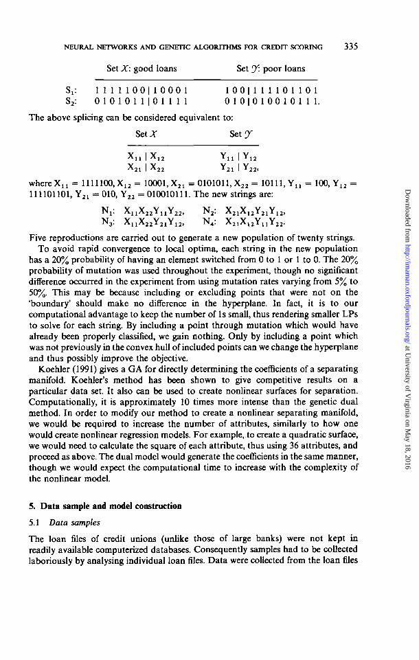
NEURAL NETWORKS AND GENETIC ALGORITHMS FOR CREDIT SCORING 335

Set X: good loans Set y-. poor loans

St: 1 1 1 1 1 0 0 | 1 0 0 0 1 1 0 0 | 1 1 1 1 0 1 1 0 1S2: 0 1 0 1 0 1 1 | 0 1 1 1 1 0 1 0 | 0 1 0 0 1 0 1 1 1 .

The above splicing can be considered equivalent to:

Set X Set J

X I Y V I V11 I A 1 2 x 11 I r 12

X I Y Y I V21 I A 2 2 X21 I r22>

where Xxl = 1111100, X12 = 10001, X21 = 0101011, X22 = 10111, Y n = 100,Y12 =111101101, Y21 = 010, Y22 = 010010111. The new strings are:

Np X11X22Y11Y22, N2: X21X12Y21Y12,N3: X11X22Y21Y12, N4: X21X12YUY22.

Five reproductions are carried out to generate a new population of twenty strings.To avoid rapid convergence to local optima, each string in the new population

has a 20% probability of having an element switched from 0 to 1 or 1 to 0. The 20%probability of mutation was used throughout the experiment, though no significantdifference occurred in the experiment from using mutation rates varying from 5% to50%. This may be because including or excluding points that were not on the'boundary' should make no difference in the hyperplane. In fact, it is to ourcomputational advantage to keep the number of Is small, thus rendering smaller LPsto solve for each string. By including a point through mutation which would havealready been properly classified, we gain nothing. Only by including a point whichwas not previously in the convex hull of included points can we change the hyperplaneand thus possibly improve the objective.

Koehler (1991) gives a GA for directly determining the coefficients of a separatingmanifold. Koehler's method has been shown to give competitive results on aparticular data set. It also can be used to create nonlinear surfaces for separation.Computationally, it is approximately 10 times more intense than the genetic dualmethod. In order to modify our method to create a nonlinear separating manifold,we would be required to increase the number of attributes, similarly to how onewould create nonlinear regression models. For example, to create a quadratic surface,we would need to calculate the square of each attribute, thus using 36 attributes, andproceed as above. The dual model would generate the coefficients in the same manner,though we would expect the computational time to increase with the complexity ofthe nonlinear model.

5. Data sample and model construction

5.1 Data samples

The loan files of credit unions (unlike those of large banks) were not kept inreadily available computerized databases. Consequently samples had to be collectedlaboriously by analysing individual loan files. Data were collected from the loan files

at University of V

irginia on May 18, 2016

http://imam

an.oxfordjournals.org/D

ownloaded from

336 V. S. DESAI ET AL.

of three credit unions in the Southeastern United States for the period 1988-91. Creditunion L is predominantly made up of teachers, and credit union N is predominantlymade up of telephone-company employees, whereas credit union M represents a morediverse state-wide sample. The narrowness of membership is somewhat mitigated bythe inclusion of family members in all three credit unions. Only credit union M hadadded select employee groups to diversify its membership.

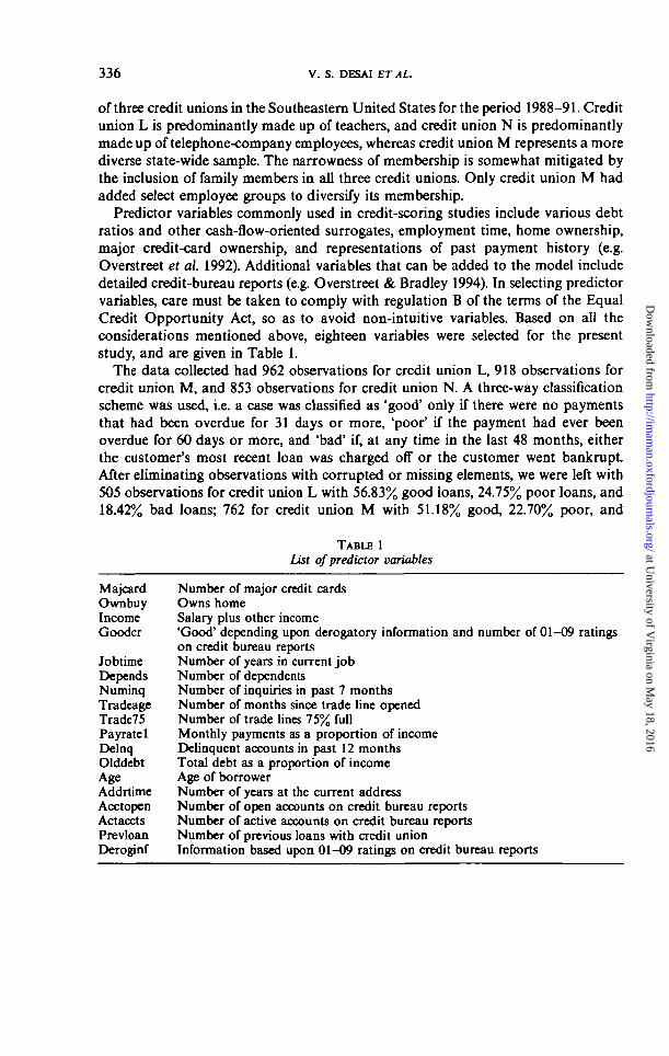
Predictor variables commonly used in credit-scoring studies include various debtratios and other cash-flow-oriented surrogates, employment time, home ownership,major credit-card ownership, and representations of past payment history (e.g.Overstreet et a\. 1992). Additional variables that can be added to the model includedetailed credit-bureau reports (e.g. Overstreet & Bradley 1994). In selecting predictorvariables, care must be taken to comply with regulation B of the terms of the EqualCredit Opportunity Act, so as to avoid non-intuitive variables. Based on all theconsiderations mentioned above, eighteen variables were selected for the presentstudy, and are given in Table 1.

The data collected had 962 observations for credit union L, 918 observations forcredit union M, and 853 observations for credit union N. A three-way classificationscheme was used, i.e. a case was classified as 'good' only if there were no paymentsthat had been overdue for 31 days or more, 'poor' if the payment had ever beenoverdue for 60 days or more, and 'bad' if, at any time in the last 48 months, eitherthe customer's most recent loan was charged off or the customer went bankruptAfter eliminating observations with corrupted or missing elements, we were left with505 observations for credit union L with 56.83% good loans, 24.75% poor loans, and18.42% bad loans; 762 for credit union M with 51.18% good, 22.70% poor, and

TABLE 1List of predictor variables

Majcard Number of major credit cardsOwnbuy Owns homeIncome Salary plus other incomeGoodcr 'Good' depending upon derogatory information and number of 01-09 ratings

on credit bureau reportsJobtime Number of years in current jobDepends Number of dependentsNuminq Number of inquiries in past 7 monthsTradeage Number of months since trade line openedTrade75 Number of trade lines 75% fullPayratel Monthly payments as a proportion of incomeDelnq Delinquent accounts in past 12 monthsOlddebt Total debt as a proportion of incomeAge Age of borrowerAddrtime Number of years at the current addressAcctopen Number of open accounts on credit bureau reportsActaccts Number of active accounts on credit bureau reportsPrevloan Number of previous loans with credit unionDeroginf Information based upon 01-09 ratings on credit bureau reports

at University of V

irginia on May 18, 2016

http://imam

an.oxfordjournals.org/D

ownloaded from

NEURAL NETWORKS AND GENETIC ALGORITHMS FOR CREDIT SCORING 337

TABLE 2

Descriptive statistics for credit union LThe number of good, poor, and bad loans equal 287,125, and 93 respectively. The first, second,and third numbers in each cell refer to the good, poor, and bad loans respectively

Variable

Majcard

Ownbuy

IncomeGoodcr

JobtimeDependsNuminqTradeage

Trade75PayratelDelnq

Olddebt

Age

AddrtimeAcctopenActacctsPrevloanDeroginf

Mean

0.659, 0.448,0.3260.714, 0.448,0.3592153, 1890, 12310.707, 0.520, 0.283

5.56, 4.67, 4.000.7, 0.9- 0.91.52, 2.60, 3.3799.53, 83.76,45.201.21,190, 2.410.33, 0.36, 0.390.335, 0.904,0.6743.33, 5.20, 4.01

37.68, 34.42,31.107.27, 6.18, 6.490.37, 0.62, 0.754.25, 5.10, 3.230.78, 0.21, 0.030.24, 0.34, 0.55

Median

1,0,0

1,0,0

1967,1429,10051, 1,0

3,2,20,0,01,2,286, 71, 30

0,3,10.30, 0.36, 0.390, 1,1

1.93, 3.16,104

37, 33, 29

4,130,0,03,4,20,0,00,0, 1

Trunc. mean

0.676, 0.443,0.3050.738, 0.443,0.34220511684,11000.730, 0.5210.2564.87, 4.10, 3.510.65, 0.78, 0.821.30, 108,17894.55, 79.1,39.790.97,162,1020J1 0.36, 0.390.317, 0.947,0.695177, 4.52, 3.29

37.09, 34.13,30.746.27, 5.17, 5.590.27, 0.50, 0.564.04, 4.74,1880.57,0.11,0.00021, 0.31 0.56

Min

0,0,0

0,0,0

548,400,4000,0,0

0,0,00,0,00,0,00,0,0

0,0,00,0,00,0,0

0,0,0

19, 18, 18

0,0,00,0,00,0,00,0,00,0,0

Max

1,1, 1

1, 1,1

9000,8368,60001, 1, 1

34,30,235,5,410, 19, 32491 288, 252

13, 20, 180.86, 0.97, 1.001, 1, 1

4139, 34.20,24.2573, 57, 49

56, 48, 404,5,616, 33, 1413, 4, 11, 1, 1

26.12% bad; and 695 observations for credit union N with 56.77% good, 22.05%poor, and 21.18% bad.

5.1.1 Descriptive data analysis. Tables 2, 3, and 4 give the descriptive statistics forthe three credit unions. Furthermore, the descriptive statistics are broken down byloan type. It is interesting to note that the median values for a number of variablesare identical for two out of three loan types, or in some instances for all loan types.For example, the median number of dependents (Depends) are equal for all threeloan types for all three credit unions, and the number of delinquent accounts in thepast 12 months (Delnq) are equal for all three loan types for credit unions M andN, and are equal for poor and bad loans for credit union L. It is also interesting tonote that the median values are identical for good and poor loans for some variablesin some credit unions, and identical for poor and bad loans for other credit unions,e.g. the number of inquiries in past 7 months (Numinq), number of open accountson credit-bureau reports (Acctopen), and the number of active accounts on credit-bureau reports (Actaccts).

5.1.2 Training and holdout data. There exist several approaches for validing statisticalmodels (e.g. Dillon & Goldstein 1984; Hair et al. 1992). The simplest approach,

at University of V

irginia on May 18, 2016

http://imam

an.oxfordjournals.org/D

ownloaded from

338 V. S. DESAI ETAL.

TABLE 3

Descriptive statistics for credit union MThe number of good, poor, and bad loans equal 390,173, and 199 respectively. The first, second,and third numbers in each cell refer to the good, poor, and bad loans respectively

Variable

Majcard

Ownbuy

Income

Goodcr

JobtimeDependsNuminqTradeage

Trade75PayratelDelnq

Olddebt

Age

AddrtimeActacctsAcctopenPrevloanDeroginf

Mean

0.628, 0.364,0.4750.746, 0.497,0.4292227,1900,1157

0.803, 0.434,0.7889.62, 4.48, 4.761.1, 1.16, 1.341.35,112,171112.84,67.56,49.680.83, 1.06, 2.970.22, 0.26, 0.400.136, 0.763,0.3792.70, 3.35, 5.35

38.72, 32.32,31.129.73, 6.71, 4.85293, 2.91, 3.920.48, 0.45, 1.13256, 207, 2560.12,0.35,0.15

Median

1,0,0

1,0,0

2016,1715,1000

1,0, 1

7.5, 2, 31, 1, 11, 1, 299, 60, 43.5

0,0,30.22, 0.26, 0.390,0,0

1.64, 268, 4.74

37, 30, 30

7,3,23,2,30,0, 12,1,30,0,0

Trunc. mean

0.643, 0.348,0.4720.774, 0.497,0.4212111,1819,1103

0.837, 0.426,0.8208.88, 3.64, 4.171.00, 1.06, 1.291.09, 1.77, 264108.08, 63.82,46.220.63, 0.87, 2840.22, 0.77, 0.990.043, 0.626,0.242227, 3.01, 4.97

38.20, 31.59,30.428.73, 5.89, 3.80279, 270, 3.760.31, 0.36, 1.05214, 1.63, 2430.07,0.33,0.11

Min

0,0,0

0,0,0

480, 538, 400

0,0,0

0,0,00,0,00,0,00,0,0

0,0,00,0,00,0,0

0,0,0

19, 19, 18

0,0,00,0,00,0,00,0,00,0,0

Max

1,1, 1

1,1, 1

10000,6000,42501, 1, 1

45, 30, 335,5,714, 16, 8409, 234, 235

9,8, 100.78, 0.77, 0.995,5,5

38.00, 17.31,27.2773,66,60

70, 53, 5512, 13, 1712,3,623, 23, 141, 1, 1

referred to as the cross-validation method, involves dividing the data into two subsets,one for training (analysis sample) and a second one for testing (holdout sample).More sophisticated approaches include the U method and the jackknife method.Both these methods are based on the 'leave-one-out' principle, where the statisticalmodel is fitted to repeatedly drawn samples of the original sample. Dillon & Goldstein(1984: p. 393) suggest that, in the case of discriminant analysis, a large standarddeviation in the estimator for misclassification probabilities can overwhelm the biasreduction achieved by the U method, and, if multivariate normality is violated, it isquestionable whether jackknifed coefficients actually represent an improvement ingeneral. Also, these methods can be computationally expensive. An intermediateapproach, and perhaps the most frequently used approach, is to divide the originalsample randomly into analysis and holdout samples several times. Given thesubstantial number of data and the fact that we investigated six models, we decidedto use an intermediate approach. The data sample was divided into two parts, withtwo thirds of the observations being used for training and the remaining one thirdfor testing. Observations were randomly assigned to the training or testing data set,and ten such pairs of data sets were created. A popular approach is to use stratifiedsampling in order to keep the proportion of good loans and bad loans identicalacross all data sets. Since the percentage of bad loans is different for the three credit

at University of V

irginia on May 18, 2016

http://imam

an.oxfordjournals.org/D

ownloaded from

NEURAL NETWORKS AND GENETIC ALGORITHMS FOR CREDIT SCORING 339

TABLE 4

Descriptive statistics for credit union NThe number of good, poor, and bad loans equal 394,153, and 148 respectively. The first, second,and third numbers in each cell refer to the good, poor, and bad loans respectively

Variable

Majcard

Ownbuy

Income

Goodcr

JobtimeDependsNuminqTradeage

Trade75PayratelDelnq

Olddebt

Age

AddrtimeAcctopenActacctsPrevloanDeroginf

Mean

0.800, 0.575,0.4490.812, 0.693,0.5442850, 2441,24100.848, 0.706,0.68713.48, 8.44, 7.4212, U 1.21.22, 208, 3.08133.23, 96.39,71.11.91,138, 2.710.29, 0.27, 0.270.368, 0.647,0.6264.49, 4.09, 4.79

38.90, 36.17,33.278.09, 8.12, 6.930.59, 0.80, 1.105.17, 4.88, 4.79Z83, 216, 2380.09, 0.16, 0.16

Median

1, 1,0

1, 1, 1

2603,2203,1950

1, 1, 1

13, 6, 51, 1, 11, 1. 1120, 79, 54

2,2,20.30, 028, 0.280,0,0

3.75, 3.85, 3.72

38, 35, 32

5,5,40,1,15,4,42,1,10,0,0

Tmnc. mean

0.833, 0.584,0.4440.846, 0.715,0.5492771, 2346, 2157

0.887, 0.730, 0.707

13.14, 7.52, 6.851.1, 1.2, 1.10.97, 1.72, 254129.91, 90.64,66.411.72, 214, 2470.29, 0.27, 0.270.220,0.511,0.4514.25, 3.91, 4.46

38, 56, 35.88,32757.42, 7.16, 5.960.49, 0.69, 0.914.95, 4.54, 4.44246, 1.82, 1.880.04, 0.12, 0.12

Min

0,0,0

0,0,0

584, 728, 600

0,0,0

0,0,00,0,00,0,00,0,0

0,0,00,0,00,0,0

0,0,0

17, 18, 18

0,0,00,0,00,0,00,0,00,0,0

Max

1, 1, 1

1, 1, 1

7499, 8500,220001, 1, 1

40, 40, 336,4,412, 15, 20342, 379, 276

10, 16, 120.91,0.62,0.606,5,8

20.57, 13.10,33.3267, 62, 69

33, 53, 415,5,922,22, 2119, 15, 251, 1, 1

unions, and since claims by practitioners imply that the performance of neuralnetworks in comparison to the conventional methods would depend upon theproportion of bad loans in the data set, we decided not to use stratified sampling,and we let the percentage of bad loans vary across the ten data sets so that ourresults would not depend upon the particular composition of the data sample athand. As Section 6 indicates, when the results were compared, we accounted for thisvariation by performing paired t tests.

5.2 Model construction

As the preceding paragraphs indicate, we want to use eighteen predictor variablesto predict whether a loan will be 'good', 'poor', or 'bad'. For the multilayerperceptron, this fixes the number of neurons in the input and output layers to eighteenand two respectively. We have used a sigmoid activation function in the hidden layer,i.e. F(z) = 1/(1 +c~r). After some preliminary testing, we decided to use a singlehidden layer starting with eighteen neurons in all our models. All models weretrained separately for each of the 10 samples for each credit union. Also, by theend of training, some models had fewer neurons than they started with, sincesome neurons were eliminated by pruning. Thus, the number of neurons deleted

at University of V

irginia on May 18, 2016

http://imam

an.oxfordjournals.org/D

ownloaded from

340 V. S. DESAI ETAL.

ranged from 0 to 10 out of the 18 neurons in the hidden layer for the MLPmodels.

For the MLP models, the initial values of the learning parameter r\ were set at0.3 for the hidden layer and 0.15 for the output layer, and the momentum parameter6 was set at 0.4 for all layers. These parameters were allowed to decay byreducing their values by half after 10,000 iterations, and again by half after 30,000iterations.

In all, the six methods tested were as follows:

Ida linear discriminant analysislr logistic regressionga genetic algorithmmlp multilayer perceptronmlp-m combination of multilayer perceptrons and a majority rulemlp-b combination of multilayer perceptrons and a best-neuron rule.

6. Comparison of results

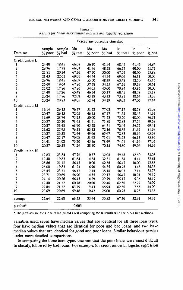
Table 5 gives the results for the traditional techniques, Table 6 does the same forneural networks and genetic algorithms, and Table 7 for combinations of neuralnetworks. For each method, the first column gives the total (i.e. the good plus thepoor plus the bad) percentage correctly classified, the second column gives thepercentage of poor loans correctly classified, and the third column gives thepercentage of bad loans correctly classified. Since the cost of giving a loan to adefaulter is far greater than rejecting a good or poor loan, the percentage of badloans correctly identified is important. Also, poor loans and good loans differ in theirprofitability. While reading the results of Tables 5-7, one must keep in mind that,in the experiments reported in the present study, we did not explicitly includemisclassification costs; this is because one of the methods, namely logistic regression,does not allow that feature. Also note that, given the information in §5.1, thepercentage of good loans correctly classified can be easily obtained from the datagiven in these tables.

6.1 Comparing credit unions

In comparing the three credit unions, one can see that models for credit union Mare the best, followed by those for credit unions L and N respectively. Given thelimited amount of information, one can only speculate as to the reasons for thesedifferences. First, M has the largest sample size, and secondly M is the only creditunion that added select employee groups to actively diversify its field of membership,indicating that the diversity of examples in the data set in terms of size and varietyis important in creating good models. However, using these factors, one would expectN to provide better results than L because L has the smallest sample size and thenarrowest field of membership. Perhaps the poor performance of N might be due tothe lack of power by the explanatory variables to separate the three groups as isindicated by the descriptive statistics for N reported in Table 4. Of the 18 explanatory

at University of V

irginia on May 18, 2016

http://imam

an.oxfordjournals.org/D

ownloaded from

NEURAL NETWORKS AND GENETIC ALGORITHMS FOR CREDIT SCORING 341

TABLE 5Results for linear discriminant analysis and logistic regression

Data set

Credit union L123456789

10

Credit union M123456789

10

Credit union N123456789

10

average

p value*

sample%poor

24.4029.7623.8121.4329.7625.6022.0224.4020.2420.24

16.1420.4719.6920.8720.8723.6220.8720.4724.4120.87

19.8319.4025.8625.0028.4523.7124.1419.4022.8420.69

22.64

sample% bad

18.4517.2820.2422.6218.4519.6417.8617.2617.8620.83

29.1329.1328.7425.2033.4827.9526.3827.1724.0226.38

23.8419.8321.1219.8323.7120.6920.2621.1221.1220.69

22.68

Percentage correctly classified

Ida% total

66.0766.0767.2669.0566.0767.8667.8665.4872.0269.05

76.77720573.2371.6568.9076.3872.4470.0875.2071.26

57.7661.6456.4761.2156.4756.9056.4760.7863.7959.48

66.53

0.003

Ida%poor

56.1041.4647.5044.4455.0057.5854.0546.3443.1852.94

51.2246.1550.0041.5145.2863.3349.0651.9245.1638.10

10.874.64

10.006.907.14

14.5514.2920.009.43

10.42

35.94

Ida% bad

41.9448.2850.0044.7448.3954.5540.0055.1743.3334.29

77.0367.5771.2371.8864.7172.4665.6771.0178.6970.15

32.0832.6142.6654.3538.1829.1729.7922.4646.9425.00

50.82

lr% total

68.4566.6767.2669.0565.4867.2670.8468.4573.8169.05

77.1771.6575.2072.8372.4476.38728373.2374.4174.80

59.4861.6456.4760.7856.03564755.17625062.5060.78

67.30

lr%poor

41.4640.0040.0036.1152.5039.3945.9548.7838.6447.06

48.7838.4648.0037.7454.7251.6750.9446.1541.9449.06

12.504.44

10.003.457.14

10.915.36

22.227.558.25

32.91

lr% bad

54.8451.7255.8850.0045.1660.6150.0055.1753.3337.14

81.0871.6276.7179.6969.4181.6965.6775.3677.0574.63

32083261428654.35327329.1736.1724.9944.9033.33

54.32

• The p values are for a one-tailed paired t test comparing the lr results with the other five methods.

variables used, seven have median values that are identical for all three loan types,four have median values that are identical for poor and bad loans, and two havemedian values that are identical for good and poor loans. Similar behaviour persistsunder more detailed comparisons.

In comparing the three loan types, one sees that the poor loans were most difficultto classify, followed by bad loans. For example, for credit union L, logistic regression

at University of V

irginia on May 18, 2016

http://imam

an.oxfordjournals.org/D

ownloaded from

342 V. S. DESAI ET AL.

TABLE 6Results for multilayer perceptrons and genetic algorithms

Data set

Credit union L123456789

10

Credit union M123456789

10

Credit union N123456789

10average

p value*

sample%poor

24.4029.7623.8121.4329.7625.6022.0224.4020.2420.24

16.1420.4719.6920.8720.8723.6220.8720.4724.4120.87

19.8319.4025.8625.0028.4523.7124.1419.4022.8420.6922.64

sample%bad

18.4517.2820.2422.6218.4519.6417.8617.2617.8620.83

29.1329.1328.7425.2033.4627.9526.3827.1724.0226.38

23.8419.8321.1219.8323.7120.6920.2621.1221.1220.6922.68

Percentage correctly classified

mlp% total

66.0770.8370.2469.4365.4860.7166.0766.6768.4563.69

77.9571.2673.6273.6270.4774.0270.8771.6572.8372.44

59.4860.3462.9359.4854.7457.7656.9061.6461.6360.3466.38

0.038

mlp%poor

48.7860.0077.5080.5628.0027.9145.9551.2376.4732.35

53.6642.3138.8849.0656.6045.0058.4951.9248.3941.51

8.692.221.671.72

14.291.821.79

17.781.892.08

35.62

mlp%bad

51.6162.0738.2415.7958.0624.2443.3355.1730.0048.57

79.7367.5769.8681.2562.3576.0665.6772.4665.5773.13

28.3036.9638.7850.0037.7835.4244.6818.3736.7335.4250.11

ga% total

63.1064.2961.9070.2467.8664.2966.6764.2969.0564.29

71.6571.2673.6271.6570.8768.5070.8768.5068.1172.83

58.6267.6755.6061.6459.9158.1956.9063.3661.6463.7965.70

0.007

ga%poor

26.8335.0030.0041.6732.0025.5837.8426.8341.1832.35

24.3936.5440.0026.4230.1928.3326.4223.0829.0335.85

26.0931.1113.3325.8623.2123.6423.2128.8920.7527.0829.19

ga% bad

74.1965.5264.7171.0570.9763.6460.0072.4166.6765.71

85.1482.4386.3085.9482.3587.3279.1084.0681.9785.07

43.4063.0459.1856.5253.3347.9255.3246.9461.2250.0068.38

* The p values are for a one-tailed paired t test comparing the lr results with the other five methods.

misclassified, on average, 57.16% of poor loans as good loans or bad loans, and30.76% of bad loans as poor loans or good loans, whereas only 14.49% of the goodloans were misclassified as poor or bad loans. These results are consistent with thedescriptive statistics reported in Tables 2-4 which show the median values of theexplanatory variables for the poor loans to be often coinciding with those for good

at University of V

irginia on May 18, 2016

http://imam

an.oxfordjournals.org/D

ownloaded from

NEURAL NETWORKS AND GENETIC ALGORITHMS FOR CREDIT SCORING 343

TABLE 7

Results for combinations of multilayer perceptrons

Data set

Credit union L123456789

10

Credit union M123456789

10

Credit union N123456789

10average

p value*

sample%poor

24.4029.7623.8121.4329.7625.6022.0224.4020.2420.24

16.1420.4719.6920.8720.8723.6220.8720.4724.4120.87

19.8319.4025.8625.0028.4523.7124.1419.4022.8420.692264

sample%bad

18.4517.2820.2422.6218.4519 6417.8617.2617.8620.83

29.1329.1328.7425.2033.4627.9526.3827.1724.0226.38

23.8419.8321.1219.8323.7120.8920.2621.1221.1220.6922.68

Percentage correctly classified

mlp-m% total

60.7167.8666.6766.0764.8861.9066.0761.3165.4860.71

78.3571.2672.4472.4469.2973.6270.4770.4773.627105

58.6251.2953.8856.0349.5752.5951.7260.3453.8860.7863.81

0.000

mlp-m%poor

29.2760.00415055.5640.0048.8351.3563.4161.7635.29

53.66413154.0041.5137.7335.0052.8350.0048.3943.40

00.0000.0000.0000.0001.7900.0010.7124.4400.0004.1732.93

mlp-m% bad

24.3955.1744.1213.1648.3921.2143.3324.1436.6745.71

79.7374.3272.60818161.1881.6971.6471.0177.0570.15

33.9617.3938.7843.4833.3314.5802.1312.2432.6514.5844.72

mlp-b% total

65.4867.8667.8669.6464.2962.5064.8866.6765.4864.88

77.5672.8874.80718371.2675.5973.62714473.2373.62

59.48615057.33615056.9058.6253.8861.2161.6460.3466.39

0.020

mlp-b%poor

41.4650.0040.0061.1138.0046.5143.2473.1758.823235

53.6651.9254.0049.0652.8355.0052.8348.0848.3950.94

13.0408.8906.6717.2407.1416.3607.1420.0005.6616.6737.00

mlp—b% bad

41.9455.1750.0023.6851.6127.2743.3334.4836.6751.43

79.73719775.3478.1264.7180.2864.18714665.5770.15

28.3041.3041865117412214.5838.3028.5736.7314.5849.29

• The p values are for a one-tailed paired t test comparing the lr results with the other five methods.

or bad loans. These results are also consistent with previous studies (e.g. Overstreet& Bradley 1995).

4.2 Comparing modelling techniques

As Tables 5-7 indicate, logistic regression identifies 67.30% of the loans correctly,which is higher than all the other models. This superiority is confirmed by a more

at University of V

irginia on May 18, 2016

http://imam

an.oxfordjournals.org/D

ownloaded from

344 V. S. DESAI ETAL.

formal comparison using a paired t test. Since the data sets differ in that theproportion of poor and bad loans were different for the ten data sets, we accountedfor this difference by using the paired t test. As the p values indicate, logistic regressionis clearly better than linear discriminant analysis and genetic algorithms, and thedifference between logistic regression and multilayer perceptrons is significant at the0.05 significance level, but not at the 0.01 significance level. The fact that logisticregression is better than discriminant analysis is consistent with results reportedelsewhere (e.g. Harrel & Lee 1985), and is perhaps due to the presence of categoricalvariables, which violates the assumption of multivariate normality required for lineardiscriminant analysis.

The situation is quite different when it comes to identifying poor and bad loanscorrectly. The combination of neural networks with the best-neuron rule (modelmlp-b) has the best performance when it comes to correctly identifying poor loans,and the genetic-algorithm models outperformed the rest when it came to correctlyidentifying bad loans. This is an encouraging result for neural networks because, asdiscussed before, poor loans are the most difficult to identify. It is worth notingthough that only linear discriminant analysis and the neural-network models usedprior probabilities of classifying the three loan types available from the trainingsamples, whereas logistic regression and genetic algorithms used equal prior prob-abilities for all three loan types. Perhaps this difference might be partially responsiblefor the higher percentage of bad loans correctly classified by logistic regression andgenetic algorithms. The fact that none of the methods are as good at identifying pooror bad loans as they are at identifying good loans seems to confirm claims bypractitioners reported in Section 1.

7. Conclusions

An attempt was made to investigate the predictive power of feedforward neuralnetworks and genetic algorithms in comparison to traditional techniques such aslinear discriminant analysis and logistic regression. A particular advantage offeredby the new techniques is that they can capture nonlinear relationships. Also, adescriptive analysis of the data suggested that classifying loans into three types—namely good, poor, and bad—might be preferable to classifying them into just goodand bad; hence the three-way classification was attempted.

Our results indicate that the traditional techniques compare very well with thetwo new techniques studied. Interestingly, neural networks performed somewhatbetter than the rest of the methods for classifying the most difficult group, namelypoor loans. The fact that the Al-based techniques did not significantly outperformthe conventional techniques suggests that perhaps the most appropriate variants ofthe techniques were not used. However, a post-experiment analysis possibly indicatesthat the reason for the new techniques not significantly outperforming the traditionaltechniques was the nonexistence of important consistent nonlinear variables in thedata sets examined.

Acknowledgements

Financial support from the Mclntire Associates Program is gratefully acknowledgedby the first author. This paper was presented at the fourth Credit Scoring and Credit

at University of V

irginia on May 18, 2016

http://imam

an.oxfordjournals.org/D

ownloaded from

NEURAL NETWORKS AND GENETIC ALGORITHMS FOR CREDIT SCORING 345

Control Conference held at the University of Edinburgh in 1995, and the authorsgratefully appreciate the comments of participants at this conference.

REFERENCES

American Banker, 1993a (29 March), p. 15A; 1993b (25 June), p. 3; 1993c (14 July), p. 3; 1993d(27 August), p. 14; 1993e (5 October), p. 14; 1994a (2 March), p. 15; 1994b (22 April), p. 17.

BOYLE, M., CROOK, J. N., HAMILTON, R., & THOMAS, L. C , 1992. Methods for credit scoringapplied to slow payers. Credit scoring and credit control (L. C. Thomas, J. N. Crook, &D. E. Edelman, Eds). Oxford University Press, Oxford. Pp. 75-90.

BRENNAN, P. J., 1993a. Promise of artificial intelligence remains elusive in banking today. BankManagement (July), pp. 49-53.

BRENNAN, P. J., 1993b. Profitability scoring comes of age. Bank Management (September),pp. 58-62.

BRYSON, A. E., & Ho, Y. C , 1969. Applied optimal control. Hemisphere Publishing, New York.CONWAY, D. G., VENKATARAMANAN, M. A., & CABOT, A. V., (forthcoming) A genetic

algorithm for discriminant analysis. Annals of Operations Research.DESAI, V. S., CROOK, J. N., & OVERSTREET JR, G. A., 1996. A comparison of neural networks

and linear scoring models in the credit union environment. European Journal ofOperational Research 95, 24-37.

DILLON, W. R., & GOLDSTEIN, M., 1984. Multivariate analysis methods and applications. Wiley,New York.

EISENBEIS, R. A., 1977. Pitfalls in the application of discriminant analysis in business, finance,and economics. Journal of Finance 32, 875-900.

EISENBEIS, R. A., 1978. Problems in applying discriminant analysis in credit scoring models.Journal of Banking & Finance 32, 205-19.

EISENBEIS, R. A., & AVERY, R. B., 1972 Discriminant analysis and classification trees. LexingtonBooks, Lexington, Massachusetts.

FAHLMAN, S. E., & LEBIERRE, C , 1990. The cascade-correlation learning architecture. Schoolof Computer Science Report CMU-CS-90-100, Carnegie Mellon University.

FISHER, R. A., 1936. The use of multiple measurement in taxonomies problems. Annals ofEugenics 7, 179-88.

FREED, N., & GLOVER, F., 1981. A linear programming approach to the discriminant problem.Decision Sciences 12, 68-74.

GREENE, W. H., 1991. LIMDEP Econometric Software Inc, New York.GILBERT, E. S., 1968. On discrimination using qualitative variables. Journal of the American

Statistical Association 63, 1399-412.GOLDBERG, D. E., 1989. Genetic algorithms in search: optimization and machine learning.

Addison-Wesley, Reading, Massachusetts.GOTHE, P., 1990. Credit bureau point scoring sheds light on shades of gray. The Credit World

(May-June), pp. 25-9.HAIR, J. F., ANDERSON, R. E., TATHAM, R. L., & BLACK, W. C , 1992. Multivariate data

analysis: eighth readings. Macmillan, New York.HANSON, S. J., & PRATT, L., 1988. A comparison of different biases for minimal network

construction with back-propagation. Advances in neural information processing systems(D. S. Touretzky, Ed.). Morgan Kaufmann, San Mateo, California. Pp. 177-85.

HANSEN, L. K., & SALAMON, P., 1990. Neural network ensembles. IEEE Transactions onPattern Analysis and Machine Intelligence 12, 993-1001.

HARRELL, F. E., & LEE, K. L., 1985. A comparison of the discrimination of discriminantanalysis and logistic regression under multivariate normality. Biostatistics: statistics inbiomedical, public health, and environmental sciences (ed. P. K. Sen). North-Holland,Amsterdam.

HAYKIN, S., 1994. Neural networks: a comprehensive foundation. Macmillan, New York.JACOBS, R. A., JORDAN, M. I., NOWLAN, S. J., & HINTON, G. E., 1991. Adaptive mixtures of

local experts. Neural Computation 3, 79-87.

at University of V

irginia on May 18, 2016

http://imam

an.oxfordjournals.org/D

ownloaded from

346 V. S. DESAI ET AL.

JOST, A., 1993. Neural networks: a logical progression in credit and marketing decisionsystems. Credit World (March/April), pp. 26-33.

KNOKE, J. D., 1982. Discriminant analysis with discrete and continuous variables. Biometrics38, 191-200.

KOEHLER, G. J., 1991. Linear discriminant function determined by genetic search. ORSAJournal of Computing 3, 345-57.

KRZANOWKI, W. J., 1977. The performance of Fisher's linear discriminant function undernon-optimal conditions. Technometrics 19, 191-200.

LACHENBRUCH, P. A., 1975. Discriminant analysis. Hafner, New York.LAPEDES, A., & FARBER, R., 1987. Non-linear signal processing using neural networks:

prediction and system modeling. Los Alamos National Laboratory report LA-UR-87-2662.

LEUNBERGER, D. G., 1969. Optimization by vector space methods. Wiley, New York.MANGASARIAN, O., 1965. Linear and nonlinear separation of patterns by linear programming.

Operations Research 13, 444-52.MOORE, D. M., 1973. Evaluation of five discrimination procedures for binary variables. Journal

of the American Statistical Association 68, 399.NILSSON, N. J., 1965. Learning machines: foundations of trainable pattern-classifying systems.

McGraw-Hill, New York.OVERSTREET JR, G. A., BRADLEY JR, E. L., & KEMP, R. S., 1992. The flat-maximum effect and

generic linear scoring model: a test. IMA Journal of Mathematics Applied in Business &Industry 4, 97-109.

OVERSTREET JR, G. A., & BRADLEY JR, E. L., 1996. Applicability of generic linear scoringmodels in the U.S. credit-union environment. IMA Journal of Mathematics Applied inBusiness & Industry 7, 291-311.

PARKER, D. B., 1982. Learning logic. Invention Report 581-64 (File 1), Stanford University,Office of Technology Licensing.

RAO, C. R., 1965. Linear statistical inference and its applications. Wiley, New York.ROBBINS, H., & MUNRO, S., 1951. A stochastic approximation method. The Annals of

Mathematical Statistics 11, 400-7.ROSENBLATT, F., Principles of newodynamics. Spartan Books, Washington D.C.RUMELHART, D. E., 1988. Learning and generalization. Proceedings of the IEEE International

Conference on Neural Networks, San Diego (Plenary address).RUMELHART, D. E., HINTON, G. E., & WILLIAMS, R. J., 1986. Learning internal representations

by error propagation. In: Parallel distributed processing: explorations in the microstructuresof cognition (D. E. Rumelhart & J. L. McCleland, Eds). The MIT Press, Cambridge,Massachusetts. Vol 1, pp. 318-62.

STEVENS, J., 1992 Applied multivariate statistics for the social sciences. Lawrence ErlbaumAssociates, New Jersey.

TAM, K. Y., & KIANG, M. Y., 1992. Managerial applications of neural networks: the case ofbank failure predictions. Management Science 38, 926—47.

TATSUOKA, M. M., 1975, Selected topics in advanced statistics, an elementary approach 6:discriminant analysis. Institute for Personality and Ability Testing, Illinois.

WERBOS, P., 1974. Beyond regression: new tools for prediction and analysis in the behavioralsciences. Unpublished Ph.D. dissertation, Harvard University, Dept. of AppliedMathematics.

WIDROW, B., 1962. Generalization and information storage in networks of adaline "neurons".In: Self-organizing systems (M. C. Yovitz, G. T. Jacobi, & G. D. Goldstein, Eds). SpartanBooks, Washington D.C. Pp. 435-61.

WEIGEND, A. S., HUBERMAN, B. A., & RUMELHART, D. E., 1990. Predicting the future: aconnectionist approach. Working Paper, Stanford University, California.

at University of V

irginia on May 18, 2016

http://imam

an.oxfordjournals.org/D

ownloaded from

View publication statsView publication stats