credit risk modelling - unibo.itcampus.unibo.it/133031/4/logit.pdfintroduction to credit risk ead...

Credit Risk Modelling

Tiziano Bellini

Università di Bologna

December 13, 2013

Tiziano Bellini (Università di Bologna) Credit Risk Modelling December 13, 2013 1 / 55

Outline Framework

Credit Risk Modelling

I Introduction to credit risk.

I Probability of default overview.

I Probability of default through GLM .

I A practical estimation of PD through R GLM.

I Concluding remarks.


Introduction to Credit Risk EAD

Exposure at Default (EAD)

EAD stands for the Exposure at Default. As a borrower goes towardsdefault it will normally attempt to increase its leverage (lend more).

I The degree in which this is possible will be dependant on the typeof products (facilities) the borrower has and the bank ability toprevent excessive draw down on facilities.

I The products can be separated into three main categories.

1. Loans.2. Working capital facilities.3. Potential exposures.



Financial Product Categories

I Loans are products where the money is made available atpredetermined moments and the customer is required to repay atpredetermined moments. Therefore there is very little theborrower can do to increase the debt.

I A working capital facility is used by a company to manage theirliquidity. The facility allows the company to borrow money up to apre-set limit. The customer is free to borrow and repay anyamount at any time as long as the total exposure remains belowthe limit.

I Potential exposure products might lead to an exposure as in thecase of a guarantee. The bank gives a guarantee for the customerto a third party. This guarantee will only translate into an exposureif this third party requests payment under the guarantee.



Working Capital and Potential Exposures

I It is necessary to specify the holding period for EAD estimation.Usually one year.

I Alternative approaches can be followed in order to estimate a kproduct factor to apply to the borrower working capital. It is usefulto distinguish between:

1. Descriptive model. A cluster analysis is carried out and the meanK factor is applied to the borrower according to its cluster.

2. Econometric model. A regression analysis is carried outconsidering dimensions such as exposure amount, geographicarea and so on.


Introduction to Credit Risk LGD

Loss Given Default (LGD)I Loss given default (LGD) represents the percentage of the EAD

which is expected to lose if a counterparty goes into default.I There are many scenarios of events which may occur after a

company goes into default. The two most extreme are as follows:1. The counterparty recovers without any loss to the bank.2. Sale of assets and collateral is required.

I Because the definition of default is rather strict (90 days overdue)many defaults will fall in the first category. Most companies whoare 90 days overdue simply recover. Often even withoutintervention by your bank.

I The sale of assets and collateral occurs less frequently but leadsto higher losses. It can be assumes that this scenario only occurswhen a company goes bankrupt. Note that bankruptcy is a lotworse than default (minimally 90 days overdue). Generally youcan separate the returns in two types:

I Return on collateralI Return on unpledged assets



LossCalc1 Mechanics

I The combination of the predictive factors is a linear weighted sum,derived using regression techniques without an intercept term.The model takes the additive form

r̂ = β1X1 + . . .+ βkXk . (1)

I r̂ is the normalized recovery.I xl is the transformed value or mini-model.I The final step is to apply a Beta-distribution transformation.

1Moody’s KMV (2005). LossCalc v2: Dynamic Prediction of LGD.Tiziano Bellini (Università di Bologna) Credit Risk Modelling December 13, 2013 7 / 55


LossCalc Factors

Figure: LossCalc Moody’s KMV explanatory factors2.

2Source: LossCalcV2.Tiziano Bellini (Università di Bologna) Credit Risk Modelling December 13, 2013 8 / 55


LossCalc Beta TransformationI Mathematically, a Beta distribution is as follows

Beta(x , α, β,Min = 0,Max) =

Γ(α + β)

Γ(α)Γ(β)

( xMax

)α−1 (1− x

Max

)β−1(

1Max

), (2)

where x is the estimated recovery rate r̂ .I The shape parameters can be derived in a variety of ways. For

example, the following give them in terms of population mean andstandard deviation

α =µ

Max

[µ(Max − µ)

Max · σ2 − 1], (3)

β = α

[Maxµ− 1]. (4)



LossCalc Drawbacks and Realized LGD

I LossCalc is not directly applicable to commercial banks becauseof the lack of market information.

I Alternative ways can be followed considering the economic LGD.The most general framework is as follows

LGDrealized = 1−∑

i Recoveryi −∑

i CostiExposure

, (5)

where the recovery is the actual value of cash flows.I Starting from the above described equation, further developments

have been carried out in practice3.

3Querci, F. Alberici, A. (2007). Rischio di Credito e Valutazione della LossGiven Default, Bancaria Editrice.Tiziano Bellini (Università di Bologna) Credit Risk Modelling December 13, 2013 10 / 55

Probability of Default Overview Introductin to PD

Introduction to PD Modelling

I The probability of default (PD), also indicated as expected defaultfrequency, is the likelihood that a loan will not be repaid and willfall into default.

I There are many alternatives for estimating the probability ofdefault. Default probabilities may be estimated exploiting:

1. Expert assessment.2. Formal (statistical) models.3. Integration of alternative approaches.

I From the source of data we distinguish among model based on:1. Non market data (balance sheet and other firm information).2. Market data (share quotations, bond spreads and so on).


Probability of Default Overview Introductin to PD

Statistical modellingI We consider as statistical those models based on data analysis

carried out through statistical tools.I Many approaches have been developed. We focus on the most

widely used in practice:1. Discriminant analysis. Developed by Altman (1968), this has been

one of the first approaches to PD estimation, but it has quickly beenquitted).

2. Logit (and GLM) regression. This is the most widely used approachexploited in commercial banks.

3. Distance to default. (This approach will be analyzed dealing withregulatory economic capital).

I There are other models such as, for example, classification andregression threes, data envelopment analysis, neural networks,. . . which are used in some area, but on the one hand they aredifficult to be interpreted and, on the other, they are not easy to beused in practice.


Probability of Default Overview Discriminant Analysis

Introduction to discriminant analysisI The main idea of discriminant analysis is to divide observations in

groups.I From a theorethical point of view, there are many approaches to

discriminant analysis. Following Fisher approach 4, we assumethat each observation belong to one of thek multivariate sampleswith the same covariance matrix.

I We etimate the group g mean from the sample and assuming∑1 = . . . =

∑k =

∑we use S to estimate

∑I We search for the linear combination Zg = a′Xg which maximizes

the separation of groups. We consider the ratio

F =SSB(a)/(k − 1)

SSW (a)/(n − k)(6)

where SSB is the variance between groups while SSW is thevariance within groups.

4Fisher, R. (1936)The Use of Multiple Measurements in TaxonomicProblems, Annals of Eugenics, 7, 179-188.Tiziano Bellini (Università di Bologna) Credit Risk Modelling December 13, 2013 13 / 55

Probability of Default Overview Discriminant Analysis

Discriminant Analysis and PD Estimation

I The ratio F is maximized when a is the eigenvector associated tothe highest eigenvalue of S−1

W SB. In the case where there aremany groups we consider many eigenvectors, while in ouranalysis, distinguishing between default and no default weconsider only one eigenvector.

I This approach is not currently used to estimate PD because:1. It can be used only in the case of numerical variables.2. It assumes

∑1 = . . . =

∑k =

∑which is not the case in our

analysis.3. It does not immediately supply a PD output.

I The use of GLM analysis allow to overwhelm these drawbacks.


Probability of Default Through GLM GLM Components

Generalized Linear Model

1. Random component. The random component of a GLM consistsof a response variable Y with independent observations(y1, . . . , yN).

2. Systematic component. The systematic component of a GLMrelates a vector(η1, . . . , ηN) to the explanatory variables through alinear model.

3. Link function. The third component of a GLM is a link functionthat connects the random and systematic components.



Random Component

I The random component of a GLM consists of a response variableY with independent observations (y1, . . . , yN) from a distribution inthe natural exponential family.

I This family has probability density function or mass function ofform

f (yi ; θi) = a(θi)b(yi)exp[yiQ(θi)]. (7)



Systematic Component

I The systematic component of a GLM relates a vector(η1, . . . , ηN)to the explanatory variables through a linear model.

I Let xij denote the value of predictor j ∈ (1, . . . ,p) for subject i .Then for all i ∈ (1, . . . ,N)

ηi =∑

j

βjxij . (8)



Link Function

I The third component of a GLM is a link function that connects therandom and systematic components.

I Let µi = E(Yi). The model links µi to ηi by ηi=g(µi), where the linkfunction g is a monotonic, differentiable function. Thus, g linksE(Yi) to explanatory variables through the formula

g(µi) =∑

j

βjxij . (9)


Probability of Default Through GLM GLM For Binary Data

Default vs Non-Default

I Let Y denote a binary response variable. In our analysis it denotesthe default or non-default of a counterparty. Each observation hasthe outcomes denoted by 0 and 1, binomial for a single trial.

I The mean E(Y ) = P(Y = 1). We denote P(Y = 1) by π(x),reflecting its dependence on values x = (x1, . . . , xp) of predictors.

I The variance of Y is

var(Y ) = π(x)[1− π(x)] (10)

which corresponds to the variance of a Bernoulli random variable.



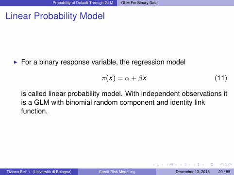
Linear Probability Model

I For a binary response variable, the regression model

π(x) = α + βx (11)

is called linear probability model. With independent observations itis a GLM with binomial random component and identity linkfunction.



Logistic Regression Model

I Usually, binary data result from a nonlinear relationship betweenπ(x) and x



Logit Link Function

I The most important curve with the above described shape is thelogistic regression model which is specified as follows

π(x) =exp(α + βx)

1 + exp(α + βx)(12)

I The link function for the logistic regression is as follows

π(x)

1− π(x)= exp(α + βx) (13)

where the log odds has the linear relationship

lnπ(x)

1− π(x)= α + βx (14)



Likelihood Equations

I We now turn our attention to details such as likelihood equationsand methods for fitting them.

I It is helpful to extend the notation for a GLM so that it can handlemany distributions that have a second parameter. The randomcomponent of the GLM specifies that the N observations(y1, . . . , yN)on Y are independent, with probability mass or densityfunction for yi of form

f (yi ; θi , φ) = exp {[yiθi − b(θi)]/a(φ) + c(yi , φ)} , (15)

that is called the exponential dispersion family and φ is called thedispersion parameter. The parameter θi is the natural parameter.



Mean and Variance for the Random Component 1/3

I We start from the contribution of Li = ln f (yi ; θi , φ) where thelog-likelihood is L =

∑i Li . Then, considering equation (15), we

obtain what follows

Li = [yiθi − b(θi)]/a(φ) + c(yi , φ). (16)

I Therefore∂Li/∂θi = [yi − b′(θi)]/a(φ), (17)

∂2Li/∂θ2i = −b′′(θi)/a(φ). (18)




I We now apply the general likelihood results

E(∂L∂θ

)= 0, (19)

−E(∂2L∂θ2

)= E

(∂L∂θ

)2

, (20)

which hold under regularity conditions satisfied by the exponentialfamily.




I From equation (19) we obtain what follows

µi = E(Yi) = b′(θi). (21)

From equation (20) we obtain what follows

b′′(θi)/a(φ) = E [(Yi − b′(θi)/a(φ)]2 = var(Yi)/[a(φ)]2, (22)

which impiesvar(Yi) = b′′(θi)a(φ). (23)



Mean and Variance for the Logit Model 1/2

I Next, suppose that niYi has a bin(ni , πi) distribution. In thiscontext, yi is the sample proportion of successes, so E(Yi) isindependent on ni . Let θi = ln[πi/(1− πi)]. Thenπi = exp(θi)/[1 + exp(θi)] and ln(1− πi) = − ln[1 + exp(θi)],therefore we can show what follows

f (yi ;πi ,ni) =

(ni

niyi

)πni yi (1− πi)

ni−ni yi =

= exp[

yiθi − ln[1 + exp(θi)]

1/ni+ ln

(ni

niyi

)]. (24)

This has exponential dispersion from equation (15) with

b(θi) = ln[1 + exp(θi)], a(φ) = 1/ni and c(yi , φ) = ln(

niniyi

).



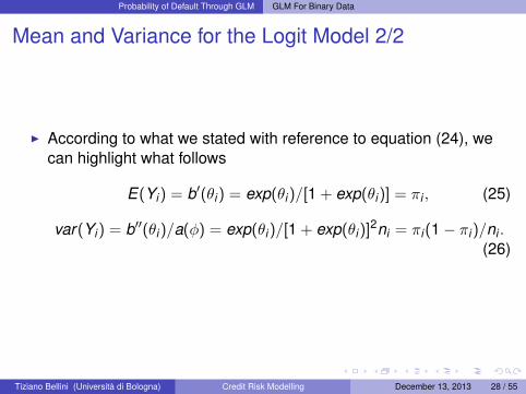
Mean and Variance for the Logit Model 2/2

I According to what we stated with reference to equation (24), wecan highlight what follows

E(Yi) = b′(θi) = exp(θi)/[1 + exp(θi)] = πi , (25)

var(Yi) = b′′(θi)/a(φ) = exp(θi)/[1 + exp(θi)]2ni = πi(1− πi)/ni .(26)



Likelihood Equations for a GLM

I For N independent observations, from equation (16), the loglikelihood is

L(β) =∑

i

Li =∑

i

ln(f (yi ; θi , φ) =∑

i

yiθi − b(θi)

a(φ)+∑

i

c(yi , φ).

(27)I The likelihood equations are

∂L(β)/∂βj =∑

i

∂L(β)/∂βj = 0, (28)

for all j .



Chain Rule

I To differentiate the log likelihood of equation (27) it is useful toexploit the chain rule

∂Li

∂βj=∂Li

∂θi

∂θi

∂µi

∂µi

∂ηi

∂ηi

∂βj. (29)

I In the above equation, ∂Li∂θi

= (yi − µi)/a(φ),∂µi∂ηi

= b′′(θ) = var(Yi)/a(φ), considering that ηi =∑

j βjxij we canstate ∂ηi

∂βj= xij and ∂µi

∂ηidepends on the link function.



Likelihood Equations

I Exploiting the above described chain rule we obtain what follows

∂Li

∂βj=

yi − µi

a(φ)

a(φ)

var(Yi)

∂µi

∂ηixij . (30)

I The likelihood equations are∑i

(yi − µi)xij

var(Yi)

∂µi

∂ηi= 0. (31)

Although the vector of βj does not appear, it is there implicitlythrough µi , since µi = g−1(

∑j βjxij).



Likelihood Equations for Binomial GLM 1/2

I Considering that niYi has a bin(ni , πi) distribution, yi is the sampleproportion of successes for ni trials. In the case of severalpredictors we have what follows

πi = Φ(∑

j

βjxij), (32)

where Φ is a generic cdf of some class of continuous distributions.I Since πi = µi = Φ(ηi) with ηi =

∑j βjxij , we can highlight that

∂µi

∂ηi= φ(ηi) = φ

∑j

βjxij

(33)



Likelihood Equations for Binomial GLM 2/2

I Since var(Yi) = πi(1− πi)/ni , the likelihood equation (31) simplifyto ∑

i

ni(yi − πi)xij

πi(1− πi)φ

∑j

βjxij

= 0. (34)

where πi = Φ(∑

j βjxij

).

I For the logit link, ηi = log[πi/(1− πi)], so ∂ηi/∂πi = 1/[pii(1− πi)]and ∂µi/∂ηi = πi(1− πi). Then, the likelihood of equation (31) and(34) simplify to ∑

i

ni(yi − πi)xij = 0, (35)

where πi satisfies equation (32) with Φ the standard logistic cdf.



Fitting GLM through Newton-Rapson and FisherScoring Methods

I The Newton-Rapson approach is an iterative method for solvingnonlinear equations. In more detail, in this context,Newton-Rapson method is exploited to obtain the value β̂ at whichthe function L(β) is maximized.

I Let u′ = (∂L/∂β1, . . . , ∂L/∂βp) and considering the Hessian matrixH, we use the notation ut and Ht to consider the t evaluation for β̂.

I Considering the Taylor series expansion

L(β) = L(βt ) + u′t (β − βt ) +

12

(β − βt )′H(β − βt ). (36)

I Fisher scoring differs from Newton-Rapson because of the use ofthe expected information (Hessian matrix) instead of the observedinformation matrix.


A Practical Estimation of PD Through R GLM GLM Regression with R

Dataset

Risposta Liquid gg_credito ROA utiliz_accord1 0 0.96 148 4.07 0.464713222 0 1.45 73 1.29 0.803552203 0 0.94 185 3.80 0.514174334 0 0.52 125 3.07 0.598729005 0 0.88 70 4.97 0.369744976 0 0.75 109 6.45 0.318675797 0 0.23 54 6.23 0.80079053...456 1 1.07 145 6.25 3.60672169457 1 0.54 88 9.71 1.19665732



Logit Regression - One Regressor

def<-as.data.frame(read.csv("110207_logit.csv",header = TRUE, sep = ";", dec="."))#log.regr.Liquid<- glm(formula=Risposta ~ Liquid, data=def,family=binomial(link=logit))summary(log.regr.Liquid)



Output of Logit Regression - One Regressor 1/2

Deviance Residuals:Min 1Q Median 3Q Max

-1.0199 -0.6164 -0.4866 -0.3741 2.6198#Coefficients:

Estimate Std. Error z value Pr(>|z|)(Intercept) -0.3008 0.3035 -0.991 0.322Liquid -2.0381 0.4437 -4.593 4.36e-06 ***



Output of Logit Regression - One Regressor 2/2

Signif. codes:0 ’***’ 0.001 ’**’ 0.01 ’*’ 0.05 ’.’ 0.1 ’ ’ 1

Null deviance: 394.75 on 456 degrees of freedomResidual deviance: 370.45 on 455 degrees of freedomAIC: 374.45#Number of Fisher Scoring iterations: 5#str(log.regr.Liquid)# in order to know all about the structure of log.regr.Liquid



ANOVA

I This looks very much like the summary of a (non-generalised)linear oneway ANOVA model, except there is no goodness-of-fit(R2).

I Instead, we are given the null deviance, which measures thevariability of the dataset, compared to the residual deviance, whichmeasures the variability of the residuals, after fitting the model.

I These deviances can be used like the total and residual sum ofsquares in a linear model to estimate the goodness of fit; this issometimes referred to as the D2 (by analogy with R2)D2<- function(mod){1-(deviance(mod)/mod$null.deviance)}D2.log.regr.Liquid<- D2(log.regr.Liquid)0.06156855



Model Fitting - One Regressor

0 100 200 300 400

0.0

0.2

0.4

0.6

0.8

1.0

sorted sample number

prob

abili

ty

fitted probability

Success of logistic model

mean probability

midpoint||||||||||

|

||||||||||||||

|

|||||||||||||||

|

||||||||||||||||||||

|

|||||||

|

||

|

|||||||||||||||||||||||||||||||||||||||||||||

|

|||||

||

||||||

|

|||||||||||||||||||||||

|

|||||||

||

|||||||||

||

|||||||

|

|||||||||||||||

|

|||||||

|

||||||||||||

|

||||||||||||||||||

|

||||||||||||||||||||||||||||||||||||||||||||

||

||||

|

|

|

|||||

|||

|

|

|||||||

|

|||

|

||||||

|

||||

||||

||||||||

|

|||||

|

||

|

|||

|||||

|||||

|

||

||

||||||||||

|

|||

|

||||

|

|

|||

|||

||

|||

|

|

||

|||

||

|

|

|||

|

||

|||||

||||

|

|||||

|

|||||||||

|

|

|

||||||

|

|||||FALSE Samples

TRUE Samples

Model: Risposta ~ LiquidAIC: 374

Null deviance: 395

Figure: Logit plot for log.regr.Liquid.



Logit Regression - Multiple Regressorslog.regr.reduced<- glm(formula=Risposta ~ Liquid+ gg_credito+ ROA +utiliz_accord,data=def, family=binomial(link=logit))#Deviance Residuals:

Min 1Q Median 3Q Max-1.95341 -0.34985 -0.14296 -0.04294 3.28233Coefficients:

Estimate Std. Error z value Pr(>|z|)(Intercept)-8.448299 1.240919 -6.808 9.89e-12 ***Liquid -2.447493 0.806733 -3.034 0.002415 **gg_credito 0.012330 0.003527 3.496 0.000473 ***ROA -0.128378 0.035866 -3.579 0.000344 ***utiliz_acco 9.668063 1.354553 7.137 9.51e-13 ***#D2.log.regr.reduced=0.4840329



Model Fitting - Multiple Regressors

0 100 200 300 400

0.0

0.2

0.4

0.6

0.8

1.0

sorted sample number

prob

abili

ty

fitted probability

Success of logistic model

mean probability

midpoint|||||||||||||||||||||||||||||||||||||||||||||||||||||||||||||||||||||||||||||||||||||||||||||||||||||||||||||

|

||||||||||

|

||||||||||||||||||||||||||||||||||||||||||||||||||||||||||||||||

|

|||||||||||||||||||||||||||||||||||

|

|||||||||||||||||||||||||||||||||||||||||||||||||||

|

||||||||

|

||||||||||||||

|

|||||||||||||||

|

|||||||||||||||||||||

|

||||||||

||

|||

||

|||||||||

|

|||||||

||

|

|

||

|

||

|

||

|

||||||

|

||

|||

||

|

||

|

||

||

||

||

||

|

|

|||||

|

|||||||||

|||

|

|

|||||||||

|

||||||||||||||||

FALSE Samples

TRUE Samples

Model: Risposta ~ Liquid + gg_credito + ROA + utiliz_accordAIC: 214

Null deviance: 395

Figure: Logit plot for log.regr.reduced.



ThresholdsI In the present example we have 457 observations, with predicted

probabilities of change from almost zero to 1. If we select athreshold of p = 0.5 (change equally likely or not), 56 (of 457) arepredicted to default. If the threshold is raised to 0.65, only 36 arepredicted to default. In fact, 71 defaulted:

I length(log.regr.reduced$fitted)457summary(log.regr.reduced$fitted)

Min. 1st Qu. Median Mean 3rd Qu. Max.7.417e-07 4.782e-03 2.899e-02 1.554e-01 1.810e-01 1.000e+00sum(log.regr.reduced$fitted > 0.5)56sum(log.regr.reduced$fitted > 0.65)36sum(def$Risposta)71



Sensitivity

I At any threshold we can compute the sensitivity and specificity, bycomparing the predicted with actual change.

I The sensitivity is defined as the ability of the model to find thepositives as follows

Sensitivity =True positivesTotal positives

. (37)

I For example, at p = 0.5, this model predicts 45 of the 71 defaults> sum((log.regr.reduced$fitted > 0.5)& def$Risposta)45sens.5 <- sum((log.regr.reduced$fitted > 0.5)& def$Risposta)/sum(def$Risposta)0.6338028



SpecificityI There is another side to a model performance: the specificity,

defined as the proportion of negatives that are correctly predicted.

Specificity =True negativesTotal negatives

. (38)

I sum(!def$Risposta)386sum(log.regr.reduced$fitted < 0.5)401sum((log.regr.reduced$fitted < 0.5)& (!def$Risposta))375spec.5 <- sum((log.regr.reduced$fitted < 0.5)& (!def$Risposta))/sum(!def$Risposta)0.9715026



False Negative Rate and False Positive Rate

I The complement of the sensitivity is the false negative rate, that is,the proportion of incorrect predictions of no change to the totalchanged. This and the sensitivity must sum to 1.

I The complement of the specificity is the false positive rate, that is,the proportion of incorrect predictions of change to the totalunchanged. This and the specificity must sum to 1.



Sensitivity vs Specificity: Threshold 0.2

100 200 300 400

0.0

0.2

0.4

0.6

0.8

1.0

prob

abili

ty o

f cha

nge

threshold = 0.2

crossover

fitted probability of change

|||||||||||||||||||||||||||||||||||||||||||||||||||||||||||||||||||||||||||||||||||||||||||||||||||||||||||||

|

||||||||||

|

||||||||||||||||||||||||||||||||||||||||||||||||||||||||||||||||

|

|||||||||||||||||||||||||||||||||||

|

|||||||||||||||||||||||||||||||||||||||||||||||||||

|

||||||||

|

||||||||||||||

|

|||||||||||||||

|

|||||||||||||||||||||

|

||||||||

||

|||

||

|||||||||

|

|||||||

||

|

|

||

|

||

|

||

|

||||||

|

||

|||

||

|

||

|

||

||

||

||

||

|

|

|||||

|

|||||||||

|||

|

|

|||||||||

|

||||||||||||||||

True negatives: 338 False positives: 48

True positives: 58False negatives: 13

Model success

Sensitivity: 0.8169 ; Specificity: 0.8756

Figure: Logit plot for log.regr.reduced. Sensitivity vs specificity.




100 200 300 400

0.0

0.2

0.4

0.6

0.8

1.0

prob

abili

ty o

f cha

nge

threshold = 0.5

crossover


|||||||||||||||||||||||||||||||||||||||||||||||||||||||||||||||||||||||||||||||||||||||||||||||||||||||||||||

|

||||||||||

|

||||||||||||||||||||||||||||||||||||||||||||||||||||||||||||||||

|

|||||||||||||||||||||||||||||||||||

|

|||||||||||||||||||||||||||||||||||||||||||||||||||

|

||||||||

|

||||||||||||||

|

|||||||||||||||

|

|||||||||||||||||||||

|

||||||||

||

|||

||

|||||||||

|

|||||||

||

|

|

||

|

||

|

||

|

||||||

|

||

|||

||

|

||

|

||

||

||

||

||

|

|

|||||

|

|||||||||

|||

|

|

|||||||||

|

||||||||||||||||



Model success






100 200 300 400

0.0

0.2

0.4

0.6

0.8

1.0

prob

abili

ty o

f cha

nge

threshold = 0.8

crossover


|||||||||||||||||||||||||||||||||||||||||||||||||||||||||||||||||||||||||||||||||||||||||||||||||||||||||||||

|

||||||||||

|

||||||||||||||||||||||||||||||||||||||||||||||||||||||||||||||||

|

|||||||||||||||||||||||||||||||||||

|

|||||||||||||||||||||||||||||||||||||||||||||||||||

|

||||||||

|

||||||||||||||

|

|||||||||||||||

|

|||||||||||||||||||||

|

||||||||

||

|||

||

|||||||||

|

|||||||

||

|

|

||

|

||

|

||

|

||||||

|

||

|||

||

|

||

|

||

||

||

||

||

|

|

|||||

|

|||||||||

|||

|

|

|||||||||

|

||||||||||||||||



Model success





ROC Curve

I A graph of the sensitivity, i.e. true positive rate (on the y-axis) vsthe false positive rate (on the x-axis) at different thresholds iscalled the Receiver Operating Characteristic (ROC) curve.

I Ideally, even at low thresholds, the model would predict most ofthe true positives with few false positives, so the curve would risequickly from (0, 0).

I The closer the curve comes to the left-hand border and then thetop border of the graph (ROC space), the more accurate is themodel; i.e. it has high sensitivity and specificity even at lowthresholds.

I The closer the curve comes to the diagonal, the less accurate isthe model. This is because the diagonal represents the randomcase.



AUC

I The ROC curve can be summarized by the area under the curve(AUC), computed by the trapezoidal rule (base times the medianaltitude)

AUC =∑

i

[xi+1 − xi ][(yi+1 + yi)/2] (39)

where the i are the thresholds where the curve is computed.I Note that the area under the diagonal is 0.5, so the ROC curve

must define an area at least that large.I The ROC area then measures the discriminating power of the

model: the success of the model in correctly classifying sites thatdid and did not actually change.

I The closer the curve comes to the diagonal, the less accurate isthe model. This is because the diagonal represents the randomcase.



ROC and AUC: One Regressor

100 200 300 400

0.0

0.2

0.4

0.6

0.8

1.0

prob

abili

ty o

f cha

nge

threshold = 0.2

crossover


||||||||||

|

||||||||||||||

|

|||||||||||||||

|

||||||||||||||||||||

|

|||||||

|

||

|

|||||||||||||||||||||||||||||||||||||||||||||

|

|||||

||

||||||

|

|||||||||||||||||||||||

|

|||||||

||

|||||||||

||

|||||||

|

|||||||||||||||

|

|||||||

|

||||||||||||

|

||||||||||||||||||

|

||||||||||||||||||||||||||||||||||||||||||||

||

||||

|

|

|

|||||

|||

|

|

|||||||

|

|||

|

||||||

|

||||

||||

||||||||

|

|||||

|

||

|

|||

|||||

|||||

|

||

||

||||||||||

|

|||

|

||||

|

|

|||

|||

||

|||

|

|

||

|||

||

|

|

|||

|

||

|||||

||||

|

|||||

|

|||||||||

|

|

|

||||||

|

|||||

True negatives: 297False positives: 89


Model success


0.0 0.2 0.4 0.6 0.8 1.00.

00.

20.

40.

60.

81.

0

(1 − specificity): false positive rate

sens

itivi

ty: t

rue

posi

tive

rate

●●●●

●●●

●●

●

●

●●

●●●

●

●●

●

●

●●●

●

●●

●

●

●●●●

●●●●●●●●●●●●●●●●●●●●●●●●●●●●●●●●●●●●●●●●●●●●●●●●●●●●●●●●●●●●●●●●●●●

Area under ROC: 0.6879

ROC One Regressor

Figure: One regressor analysis.



ROC and AUC: Multiple Regressor

100 200 300 400

0.0

0.2

0.4

0.6

0.8

1.0

prob

abili

ty o

f cha

nge

threshold = 0.2

crossover


|||||||||||||||||||||||||||||||||||||||||||||||||||||||||||||||||||||||||||||||||||||||||||||||||||||||||||||

|

||||||||||

|

||||||||||||||||||||||||||||||||||||||||||||||||||||||||||||||||

|

|||||||||||||||||||||||||||||||||||

|

|||||||||||||||||||||||||||||||||||||||||||||||||||

|

||||||||

|

||||||||||||||

|

|||||||||||||||

|

|||||||||||||||||||||

|

||||||||

||

|||

||

|||||||||

|

|||||||

||

|

|

||

|

||

|

||

|

||||||

|

||

|||

||

|

||

|

||

||

||

||

||

|

|

|||||

|

|||||||||

|||

|

|

|||||||||

|

||||||||||||||||

True negatives: 338False positives: 48


Model success


0.0 0.2 0.4 0.6 0.8 1.00.

00.

20.

40.

60.

81.

0

(1 − specificity): false positive rate

sens

itivi

ty: t

rue

posi

tive

rate

●●

●●●●●●

●●●●●●●●

●●●

●●●●●●●●

●●●●●●●●●●●●●

●●●●●●●●●●●●●●●●●

●●●●●●●●●●●●●●●●●●●●●●●●

●●●●●●●●●●●●●●●●●●

●

Area under ROC: 0.9173

ROC Multiple Regressors

Figure: Multiple regressors analysis.


Concluding Remarks Summary

Conclusions

I We introduced credit risk factors.

I We summarized how to estimate EAD and LGD.

I We analyzed in more detail PD considering alternativeapproaches.

I We introduced GLM and R software to estimate PDs on real data.


Concluding Remarks References

ReferencesI Agresti, A. (2002). Categorical Data Analysis, Wiley, Hoboken, New

Jersey.I Altman, E.I.(1968). Financial Ratios, Discriminant Analysis and the

Prediction of Corporate Bankruptcy, Journal of Finance, 23, 589-609.I Altman, E.I., Brady, B., Resti, A., Sironi, A. (2003). The Link between

Default and Recovery Rates: Theory, Empirical Evidence andImplications, Working Paper.

I Atkinson, A.C., Riani, M., Cerioli, A. (2004). Exploring Multivariate Datawith the Forward Search, Springer-Verlag, New York.

I Fisher, R. (1936)The Use of Multiple Measurements in TaxonomicProblems, Annals of Eugenics, 7, 179-188.

I Grossi, L., Bellini, T. (2006). Credit Risk Management through RobustGeneralized Linear Models. Data Analysis, Classification and theForward Search, 377-386.

I Moody’s KMV (2005). LossCalc v2: Dynamic Prediction of LGD.I Querci, F., Alberici, A. (2007). Rischio di Credito e Valutazione della

Loss Given Default, Bancaria Editrice.


credit risk modelling - unibo.itcampus.unibo.it/133031/4/logit.pdfintroduction to credit risk ead...

Documents