credit risk modelling and analysis in practice · credit risk modelling and analysis in practice...

W.Mussil / CRM 2001 - February 1st, 2001

Credit Risk Modellingand Analysis in Practice

DI Walter MUSSIL

Bank Austria AG

[email protected]

CRM 2001

Vienna, February 1st, 2001

Abbreviated Handout Version


Overview

- Basic concepts

- Level 1: The rating model

- Level 2: The portfolio model

- Sidestep: Using simulation models - Parameter effects

- Portfolio management


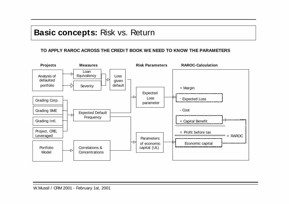
Basic concepts: Risk vs. Return

TO APPLY RAROC ACROSS THE CREDIT BOOK WE NEED TO KNOW THE PARAMETERS

+ Margin

Expected Loss

- Cost

+ Capital Benefit

= Profit before tax

Economic capital

-

= RAROC

Analysis of

portfoliodefaulted

Severity

Loan Equivalency Loss

given default

of economicParameters

capital (UL)

Lossparameter

Expected

Projects Measures Risk Parameters RAROC-Calculation

Grading Corp.

Expected DefaultFrequency

Correlations &Concentrations

Grading Intl.

Project, CRE,Leveraged

PortfolioModel

Grading SME


Level 1 - The rating model: Major steps

1) Analysis of portfolio / Requirements

2) Building of model

3) Implementation / Institutionalization


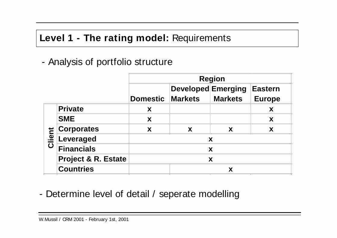
Level 1 - The rating model: Requirements

- Analysis of portfolio structure

- Determine level of detail / seperate modelling

DomesticDeveloped Markets

Emerging Markets

Eastern Europe

Private x xSME x xCorporates x x x xLeveragedFinancialsProject & R. EstateCountries x

Clie

nt

Region

xxx


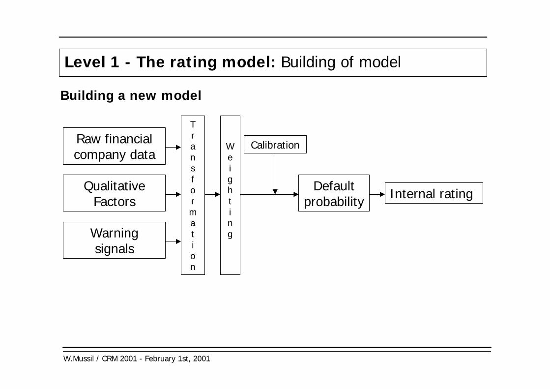
Level 1 - The rating model: Building of model

Raw financialcompany data

Defaultprobability

Calibration

Internal rating

Weighting

The short way: calibrating the old model


0.01

0.10

1

10

100

EDF

RatingR1 R2 R3 R4 R5


But: Usually large overlaps can be observed



Defaultprobability

Calibration

Internal rating

Raw financialcompany data

QualitativeFactors

Warningsignals

Weighting

Transformation

Building a new model


DATA-COLLECTION

SINGLE-FACTOR

ANALYSIS

FACTOR-COMBINATIONS

(CORRELATIONS)

WEIGHTINGand TEST

CALIBRATION

- Customer Data- External Data- Rating-Agencies

- Selection / Definition- Analysis of discriminatory power

-> Short list

- Elimination of highlycorrelated factors

-> opt.combination

- Determination of factor weightings

- Test

- Calibration tomaster scale

Level 1 - The rating model: Building process

The necessary steps for building a statistical rating model are:


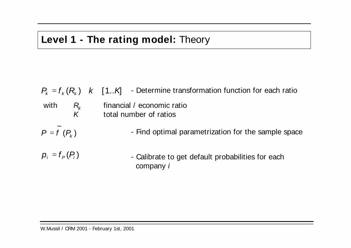
Level 1 - The rating model: Theory

[1..K]kRfP kkk ∈∀= )(

)(~

kPfP =

)( iPi Pfp =

- Determine transformation function for each ratio

- Calibrate to get default probabilities for each company i

- Find optimal parametrization for the sample space

with Rk financial / economic ratioK total number of ratios


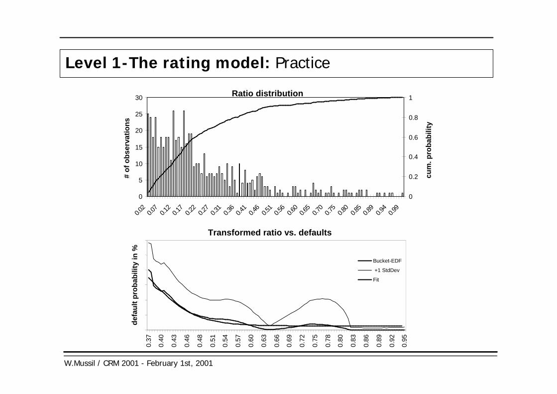
Level 1-The rating model: Practice

0

5

10

15

20

25

30

0.02

0.07

0.12

0.17

0.22

0.27

0.31

0.36

0.41

0.46

0.51

0.56

0.60

0.65

0.70

0.75

0.80

0.85

0.89

0.94

0.99

0

0.2

0.4

0.6

0.8

1Ratio distribution

Transformed ratio vs. defaults

# of

obs

erva

tions

defa

ult p

roba

bilit

y in

%

cum

. pro

babi

lity

0.37

0.40

0.43

0.46

0.48

0.51

0.54

0.57

0.60

0.63

0.66

0.69

0.72

0.75

0.78

0.80

0.83

0.86

0.89

0.92

0.95

Bucket-EDF

+1 StdDev

Fit


STATISTICAL ANALYSIS:

Measure predictive power of single factors

Identify optimal weights for combining highly predictive and economically important factors (multi-linearregressions)

Compare various models withhigh discriminatory power,according to economic criteria

EXPERT DISCUSSIONS:

- Accounting Experts- Research Group- Risk Management- External benchmarks - Experience

. . . SINCE THERE EXISTS LIMITED DATA, EXPERT DISCUSSIONS PLAY AN ESSENTIAL ROLE

Level 1 - The rating model: Building processThe rating system should be the result of a combination ofstatistical analysis and expert discussions ...


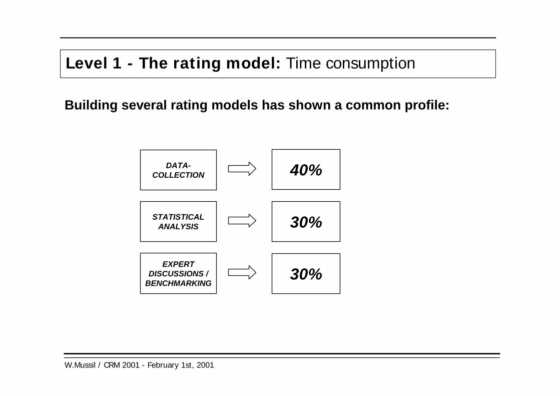
DATA-COLLECTION

STATISTICALANALYSIS

40%

Level 1 - The rating model: Time consumption

Building several rating models has shown a common profile:

EXPERTDISCUSSIONS /

BENCHMARKING

30%

30%


Level 1 - The rating model: Implementation

A) Building of IT-application:- centralized data warehouse in uniform format- modular system

- usage throughout the whole bank

B) Definition of "Rating Rules" (guideline)

C) Installation of rating-process

Time Horizon: 7 - 9 months


Level 2 - The portfolio model: Major steps

1) Specification of portfolio-model

2) Data collection

3) Parametrization

4) Prototype for reconciliation and structuring

5) Implementation and reporting


MODELSPEZIFICATION

DATACOLLECTION

20%

Level 2 - The portfolio model: Time consumption

Data collection and parametrization are the most important steps

EXPERTDISCUSSIONS

40%

10%

PARAMETRIZATION 30%


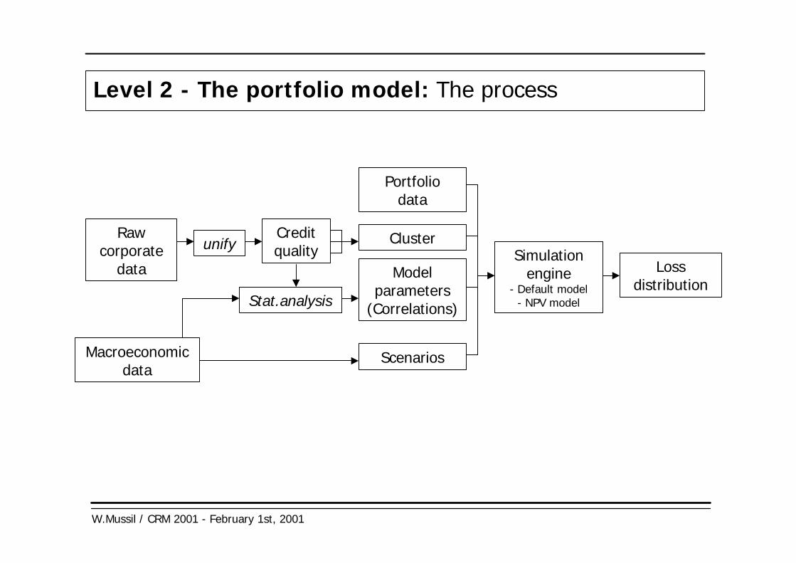
Level 2 - The portfolio model: The process

Portfoliodata

Rawcorporate

data

ClusterCreditqualityunify

Stat.analysis

Modelparameters

(Correlations)

Macroeconomicdata

Scenarios

Simulationengine

- Default model- NPV model

Lossdistribution


Level 2 - The portfolio model: Theory part 1

{ }ttp ii ≤= τPr)(

( )ii p1−=χ

- Start with the unconditional default probability of obligor i ...

... and transform it into an unconditional credit quality

- A change in orthogonal economic factor returns mj results in a change in credit quality ...

... which leads to a conditional default probability for each scenario

, with τi time of default

∑

∑−=

⋅+⋅==

2

1

1

]1,0[~,;)())(|(

iji

ii

M

jjiji Niidmtmtmt

βσ

εεσβδ

{ }

⋅−=≤= ∑

i

iiii

tmtmttmtp

σβχ

τ )()(|Pr))(|(

Φ

Φ


Level 2 - The portfolio model: Clustering

Comp 1

Comp 2

Comp n

.

.

.

.

.

.

.

.

Time serie for each company

Cluster 1

Cluster 2

Cluster m

.

.

.

.

C_1

C_2

C_m

Time serie for each cluster

Transformation

Grouping

- Grouping companies into clusters reduces complexity dramatically


Level 2 - The portfolio model: Macroeconomic factors

-2.5

-2.0

-1.5

-1.0

-0.5

0.0

0.5

1.0

1.5

2.0

2.5

3.0

Dec

-91

Jun-

92

Dec

-92

Jun-

93

Dec

-93

Jun-

94

Dec

-94

Jun-

95

Dec

-95

Jun-

96

Dec

-96

Jun-

97

Dec

-97

Actual

Predicted

Change in Credit Quality

Clusters responded well to the macro-economy


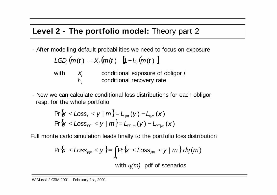
Level 2 - The portfolio model: Theory part 2

( ) ( ) ( )[ ])(1)()( tmtmXtmLGD iii η−⋅=- After modelling default probabilities we need to focus on exposure

with Xi conditional exposure of obligor iηi conditional recovery rate

- Now we can calculate conditional loss distributions for each obligor resp. for the whole portfolio

Full monte carlo simulation leads finally to the portfolio loss distribution

{ } )()(|Pr || xLyLmyLossx mimii −=<<{ } )()(|Pr || xLyLmyLossx mPFmPFPF −=<<

with θ(m) pdf of scenarios

{ } { }∫ <<=<<m

PFPF mdmyLossxyLossx )(|PrPr θ


Level 2 - The portfolio model: Simulation Framework

INPUTDATA

CLIENT /CLUSTERCHARACTERISTICS

• Exposure• Colleterals• Margin• Rating

• Factorweights

FACTOR-CORRELATIONS

MONTE-CARLO SIMULATION

SZENARIO 1PORTFOLIO-REACTION

T O SZENARIO

DEquityDFX

DUnemp

==••=

-20%+5%

+2%

SZENARIO 2

SZENARIO 3

•

•

SZENARIO N*

DEquityDFX

DUnemp

==••=

+15%+0.5%

-0.5%

% C hange in Value, % Losses

Probability Density

•

••

Probability Density

% C hange in Value, % Losses

The loss distribution is generated with a Monte-Carlo-Simulation of theunderlying macro factors

5.00%0.00%-5.00%-10.00%

SIMULATED LOSS- &NPV-DISTRIBUTION

%NPV-Change, % Loss

Probability

Loss

NPV


Sidestep - Using simulation models

To determine complete loss distribution:

- Usually calculation of 10.000s scenarios necessary (even with sophisticated sampling techniques)

⇒ compared to analytical solutions a little more time consuming

But: - Calculation can easily be "distributed"- Results are much more transparent- Illiquid portfolios can be modelled- Much higher flexibility



Using intranet-technology increases speed enormously...

Client 1 Virtual parallel computing

Client 4

Client 3

Client 2

Server 2

C1

C4

C2

C3

Server 1



- A Client-Server-Client concept coordinates calculations throughout the whole network

Client 1

Client 4

Client 3

Client 2

Server 2

C1

C4

C2

C3

Server 1



Each scenario leads to a conditional expected and unexpected loss


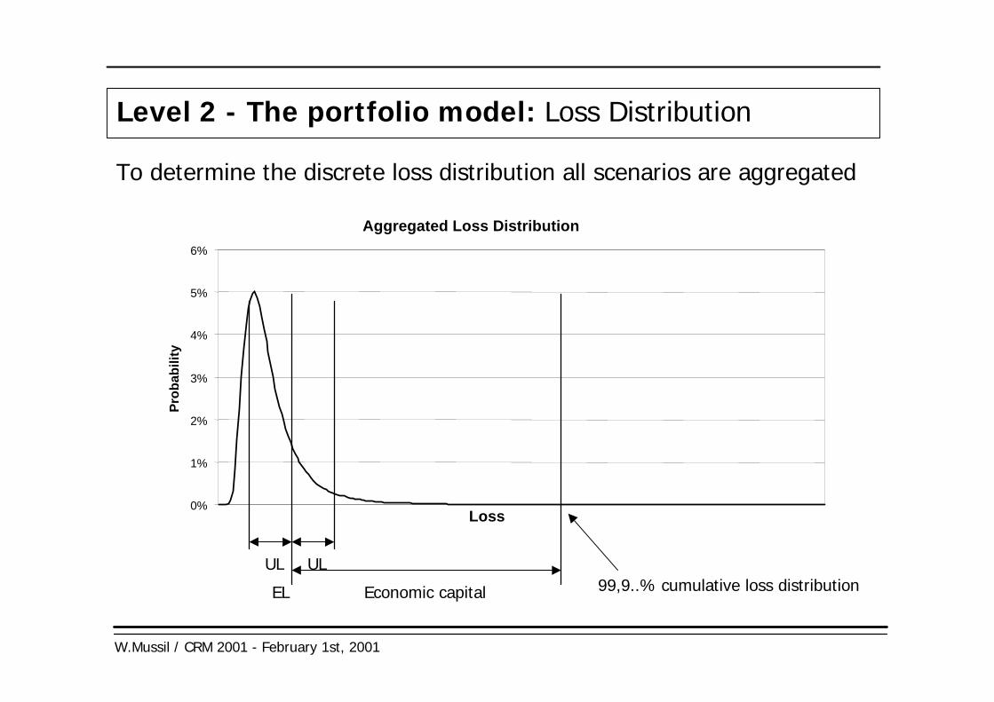
Level 2 - The portfolio model: Loss Distribution

To determine the discrete loss distribution all scenarios are aggregated

ELULUL

Economic capital 99,9..% cumulative loss distribution

Aggregated Loss Distribution

0%

1%

2%

3%

4%

5%

6%

Pro

babi

lity

Loss


Level 2 - The portfolio model: Sensitivity Analysis

Dramatic changes in macro-economic factors can result in extremelyhigh losses.

Conditional Loss x.x%Probability 0.25% (1x all 400 years)

Loss

S&P +xx%Trade-weighted EURO +xx%Raw materials index -xx%EURO ST-IR +x,x% absolut


Parameter effects: EDF

Sample calculations help to point out influences of parametrization...

0,0%

0,2%

0,4%

0,6%

0,8%

1,0%

1,2%

1,4%

1,6%

0% 1% 2% 3% 4% 5% 6% 7%

EDF -10%

EDF +10%base case

EL UL Capital AA1,49% 0,82% 6,08%1,66% 0,88% 6,39%1,83% 0,93% 6,66%

Sample portfolio size: 300 Mrd ATS


Parameter effects: Correlation vs. stochastic severity

Changes in correlation also have high impact on UL and capital ...

avg rho asset UL AA -10% rel.chg 17% 0,83% 5,85%base case 19% 0,88% 6,39% +10% rel.chg 21% 0,93% 6,93%high level 50% 2,68% 26,63%even higher level 80% 4,03% 42,65%

σSEV UL AA

0% 0,880% 6,39%30% 0,882% 6,39%50% 0,885% 6,41%

... but modelling volatility of severity has only small effects


Portfolio Management: RAROC I

xx%

xx%

xx%

xx%

Ind A

Ind B

Ind C

Ind E

Ind D

Ind L

Ind KInd JInd HInd GInd F Ind I

RAROC

Economic Capital (ATS bn)

Analysis of different industry-segments shows us clearly the loss leaders.


Portfolio Management: RAROC II

xx%

xx%

xx%

Capital (ATS bn)

RAROC %

R1 R2 R3 R4 R5 RATING

Risk adjusted profitability looks similar across and within rating classes.


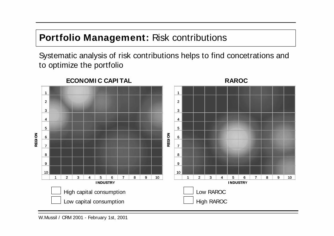
Portfolio Management: Risk contributions

Systematic analysis of risk contributions helps to find concetrations andto optimize the portfolio

1

2

3

4

5

6

7

8

9

101 2 3 4 5 6 7 8 9 10

INDUSTR

REGI

ON

1

2

3

4

5

6

7

8

9

101 2 3 4 5 6 7 8 9 10

INDUSTRY

REGI

ON

ECONOMIC CAPITAL

High capital consumptionLow capital consumption

1

2

3

4

5

6

7

8

9

101 2 3 4 5 6 7 8 9 10

INDUSTR

REGI

ON

1

2

3

4

5

6

7

8

9

101 2 3 4 5 6 7 8 9 10

INDUSTRY

REGI

ON

RAROC

Low RAROCHigh RAROC


Portfolio Management: A „real“ sample picture

Sample snapshot of BA - credit risk portfolio application


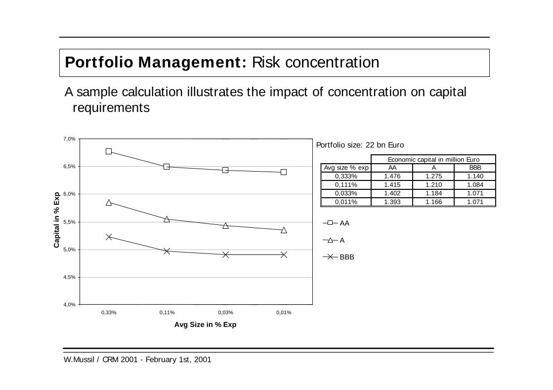
A sample calculation illustrates the impact of concentration on capital requirements

Portfolio Management: Risk concentration

4,0%

4,5%

5,0%

5,5%

6,0%

6,5%

7,0%

0,33% 0,11% 0,03% 0,01%

Avg Size in % Exp

Cap

ital i

n %

Exp

AA

A

BBB

Avg size % exp AA A BBB

0,111% 1.415 1.210 1.0840,033% 1.402 1.184 1.0710,011% 1.393 1.166 1.071

Economic capital in million Euro

0,333% 1.476 1.275 1.140

Portfolio size: 22 bn Euro


0,01% 0,03% 0,1% 0,3%1% 3%

0%

1%

10%

0x%

1x%

2x%

3x%

4x%

5x%

Margin

% Exposure

EDF

To reach the same level of RAROC concentration effects need to beconsidered in pricing

Portfolio Management: Pricing


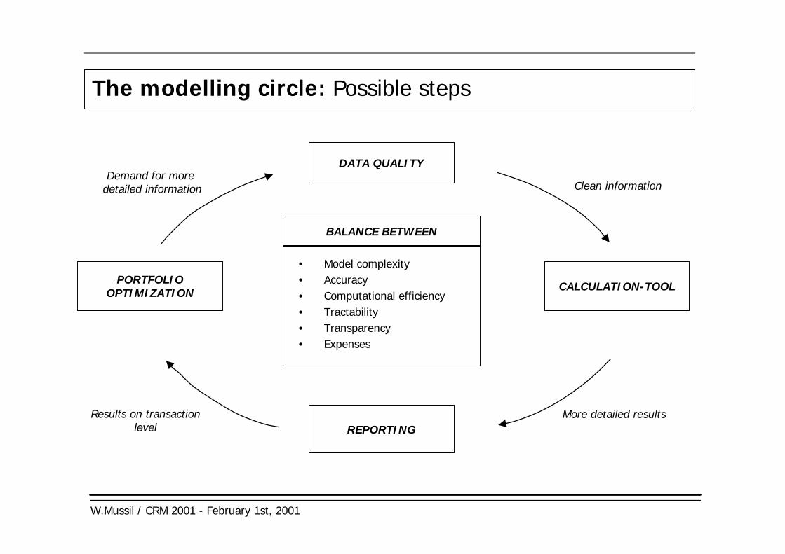
The modelling circle: Possible steps

PORTFOLIOOPTIMIZATION

DATA QUALITY

CALCULATION-TOOL

REPORTING

Clean information

More detailed resultsResults on transactionlevel

Demand for more detailed information

BALANCE BETWEEN

• Model complexity• Accuracy• Computational efficiency• Tractability• Transparency• Expenses


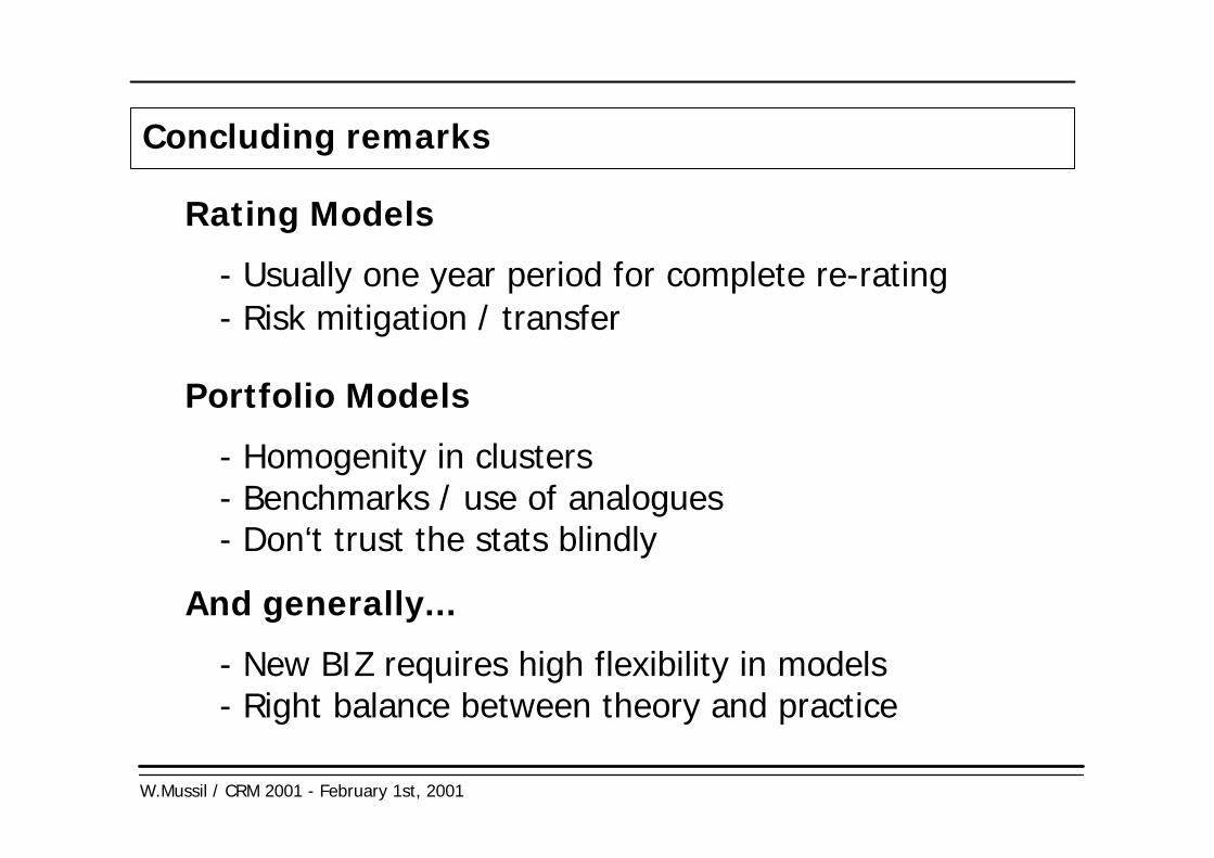
Concluding remarks

Rating Models- Usually one year period for complete re-rating- Risk mitigation / transfer

Portfolio Models- Homogenity in clusters- Benchmarks / use of analogues- Don‘t trust the stats blindly

And generally...- New BIZ requires high flexibility in models- Right balance between theory and practice

credit risk modelling and analysis in practice · credit risk modelling and analysis in practice...

Documents