Electronic copy available at: http://ssrn.com/abstract=2022279

Credit Lines as Monitored Liquidity Insurance: Theoryand Evidence*

Viral Acharyaa;y, Heitor Almeidab, Filippo Ippolitoc, Ander Perezd

a New York University, CEPR & NBER, 44 West Fourth Street, New York, NY 10012-1126, USAb University of Illinois & NBER, 4037 BIF, 515 East Gregory Drive, Champaign, IL, 61820, USAc, d Universitat Pompeu Fabra & Barcelona GSE, Ramon Trias Fargas, 25-27, 08005 Barcelona, Spain

Abstract

We propose and test a theory of corporate liquidity management in which credit lines provided bybanks to �rms are a form of monitored liquidity insurance. Bank monitoring and resulting credit linerevocations help control illiquidity-seeking behavior by �rms. Firms with high liquidity risk are likelyto use cash rather than credit lines for liquidity management because the cost of monitored liquidityinsurance increases with liquidity risk. We exploit a quasi-experiment around the downgrade ofGeneral Motors (GM) and Ford in 2005 and �nd that �rms that experienced an exogenous increasein liquidity risk (speci�cally, �rms that were rated and that relied on bonds for �nancing in thepre-downgrade period) moved out of credit lines and into cash holdings in the aftermath of thedowngrade. We also �nd support for the model�s novel empirical implication that �rms with lowhedging needs (high correlation between cash �ows and investment opportunities) are more likelyto use credit lines relative to cash, and are also less likely to face covenants and revocations whenusing credit lines.

Key words: Liquidity management, cash holdings, liquidity risk, covenants, loan commitments, creditline revocationJEL classi�cation: G21, G31, G32, E22, E5.

* We are grateful to Igor Cunha and Ping Liu for excellent research assistance and for comments from FrancoisDeGeorge (discussant) and seminar participants at the European Finance Association (EFA) Meetings, 2012,the European Central Bank, Georgia State University, ESADE, la Caixa, Universidade Nova de Lisboa,University of Technology Sydney and University of New South Wales for comments and suggestions.y Corresponding author. Email addresses: vacharya@stern.nyu.edu (V. Acharya), halmeida@illinois.edu (H.Almeida), �lippo.ippolito@upf.edu (F. Ippolito), ander.perez@upf.edu (A. Perez)

Electronic copy available at: http://ssrn.com/abstract=2022279

1 Introduction

Theory suggests that the main di¤erence between a credit line and standard debt is that a

credit line allows the �rm to access pre-committed debt capacity (e.g., Holmstrom and Tirole

(1997, 1998) and Shockley and Thakor (1997)). This pre-commitment creates value for credit

lines as a corporate liquidity management tool, in that they help insulate the corporation

from negative shocks that may hinder access to capital markets. In particular, credit lines

can be an e¤ective, and likely cheaper substitute for corporate cash holdings. Nevertheless, the

results in Su� (2009) challenge the notion that credit lines have perfect commitment. Access

to credit lines is often restricted precisely when the �rm needs it most, that is, following

negative pro�tability shocks that cause contractual covenant violations. In addition, the

survey evidence in Lins, Servaes and Tufano (2010) suggests that corporate CFOs do not

always use credit lines as precautionary savings against negative pro�tability shocks, but also

to help fund future growth opportunities.

We propose and test a theory of corporate liquidity management that bridges the gap

between existing theory and empirical evidence on credit lines. This theory explains how

credit line revocation following negative pro�tability shocks can be optimal, and it shows

when the presence of future growth opportunities may induce �rms to use credit lines in their

liquidity management. The theory generates empirical predictions that we test using a novel

dataset on credit lines, and a new identi�cation strategy.

In the model, a fully committed credit line (that is, full and irrevocable liquidity insurance)

creates the following problem. While it protects �rms from value-destroying pro�tability

shocks, once full insurance is in place �rms may gain incentives to engage in risky investments

that increase the risk of liquidity shocks (�illiquidity transformation�). Bank-provided credit

lines can help eliminate the �rm�s incentive to engage in illiquidity transformation, because

the bank retains the right (through credit line covenants, for example) to revoke access to the

credit line if it obtains a signal that the �rm may have engaged in illiquidity transformation.

Crucially, bank monitoring and line revocation tend to happen in the same states in which the

�rm needs the credit line the most (liquidity-shock states). This coincidence arises because

credit line drawdowns are negative NPV loans for the bank. Thus, the bank�s incentive

to monitor is strongest precisely when the �rm attempts to draw on the credit line. And,

in this way, credit line revocation provides incentives both for the �rm to avoid illiquidity

transformation, and for the bank to pay monitoring costs.

In this framework, the cost of credit line-provided liquidity insurance arises not only from

direct monitoring costs, but also because credit line revocations cause the �rm to pass on

1

Electronic copy available at: http://ssrn.com/abstract=2022279

valuable investments. In equilibrium, �rms may then choose to switch to cash holdings if the

cost of credit lines is too high. In particular, the model points to an important determinant

of the choice between cash and credit lines - the �rm�s total liquidity risk. Firms with greater

liquidity risk are monitored more often, causing direct and indirect monitoring costs (i.e.,

expected costs of credit line revocation) to increase, and as a result are particularly likely to

forego monitored liquidity insurance and to switch to self-insurance (cash holdings).

We extend the model to allow �rms to demand liquidity not only to absorb negative prof-

itability shocks, but also to pursue additional investment opportunities. The �nancing of

future investments interacts with liquidity shock insurance through two channels. First, the

cost of credit line revocation increases because credit line revocation both limits the contin-

uation of existing projects, and stops the �rm from undertaking new investments. Second,

future growth opportunities may provide incentives for �rms to avoid illiquidity transforma-

tion independently of monitoring. The �rst channel is particularly relevant for �rms that

tend to have investment opportunities in states with low cash �ows (in which credit lines are

likely to be revoked). The second channel is particularly relevant for �rms that tend to have

investment opportunities in high cash �ow states (whose probability decreases with illiquid-

ity transformation). This set up implies that �rms with low hedging needs (high correlation

between cash �ows and investment opportunities) are less likely to use cash relative to credit

lines, and are also less likely to require credit line covenants and revocation when using credit

lines for liquidity insurance.

Overall, our model provides two sets of empirically testable predictions, one set dealing

with the relationship between liquidity risk and liquidity management, and another set dealing

with the relationship between hedging needs, liquidity management, and credit line covenants

and revocations. We test these predictions using a novel dataset on credit lines from Capital

IQ (CIQ). The data cover a large sample of �rms in the United States for the period of 2002

to 2011. CIQ compiles detailed information on capital structure and debt structure by going

through �nancial footnotes contained in �rms� 10-K Securities and Exchange Commission

(SEC) �lings. In particular, CIQ contains detailed information on the drawn and undrawn

portions of lines of credit.

We test the implication that an increase in liquidity risk decreases reliance on credit lines

by exploiting a quasi-experiment: the downgrade of General Motors (GM) and Ford in 2005.

The downgrade came as an exogenous and unexpected shock, especially for �rms not in the

auto sector. Acharya, Schaefer and Zhang (2008) examine the GM-Ford downgrade in detail,

and show that it led to a market-wide sell-o¤ of the corporate bonds issued by these two �rms.

The downgrade had a signi�cant impact on inventory risk faced by �nancial intermediaries

2

that operated as market makers for the securities issued by the two auto makers. The resulting

e¤ect on corporate bond prices went beyond the bonds of GM and Ford and of other producers

in the auto sector, creating a widespread increase in liquidity risk that a¤ected �rms that relied

on publicly-traded bonds for their �nancing.

Consistent with the model�s predictions, we �nd that �treated� �rms that experienced

an exogenous increase in liquidity risk due to the GM-Ford downgrade �speci�cally, �rms

that were rated and that relied on bonds for �nancing in the pre-downgrade period �moved

out of credit lines and into cash holdings in the aftermath of the downgrade, relative to the

set of �control��rms. More speci�cally, we �nd that while "treated" �rms had on average

around 5% less cash holdings as a share of total liquidity relative to "control" �rms before the

GM-Ford downgrade, following the downgrade their cash holdings were on average around

2% higher as a share of total liquidity relative to "control" �rms. A placebo test in a period

outside of the downgrade episode reveals no such e¤ect. Further, we �nd that there is both

an increase in cash holdings and a decrease in credit line usage for the �treated��rms relative

to the �control��rms.

Next, we provide novel evidence linking corporate hedging needs to liquidity management

and credit line contracting. Following existing literature (Acharya, Almeida and Campello

(2007) and Duchin (2010)), we measure hedging needs by correlating �rm cash �ows with in-

vestment opportunities. We measure investment opportunities using two alternative industry-

level proxies, median industry annual investment activities and median industry Tobin�s Q.

In addition we collect information from LPC Dealscan on covenants attached to new credit

lines issued to the �rms in our sample.

In line with the predictions of our model, we �nd that low-hedging needs �rms (those with

the highest correlations between cash �ows and investment opportunities) are the most likely

to use credit lines. Depending on the measure chosen, moving from the bottom quintile to

the top quintile of hedging-needs is associated on average with a decrease of between 17% and

19% in the probability of having a line of credit, holding other variables constant. The credit

lines of low hedging-needs �rms are also less likely to contain covenants, and to be revoked

by banks. These �ndings support the model�s implications that credit lines are less costly for

low-hedging needs �rms, and that for such �rms, the credit line provider (the bank) is less

likely to retain revocation rights through covenants and to exercise them. In particular, these

�ndings stem uniquely from the feature of our model that �rms taking out lines of credit are

monitored by banks that provide the lines by inclusion of contract terms such as covenants and

by invoking them ex post; the high expected cost of monitoring and the ex-post revocation

costs for high-hedging needs �rms (which face a greater illiquidity transformation problem)

3

induce these �rms in equilibrium to rely more on cash rather than on lines of credit.

While we see the new identi�cation strategy for the liquidity risk tests and the hedging

needs tests (which together provide support for lines of credit being a form of monitored

�nance) as the main empirical contributions of the paper, we show that our results are also

consistent with existing empirical evidence. Our main goal is to show that the Capital IQ data

delivers results that closely resemble those obtained with other datasets. For example, Capital

IQ data con�rm earlier �ndings that pro�table, safer, low Q and high tangibility �rms are

more likely to have credit lines and less likely to use cash for liquidity management. Credit line

users tend to have higher bond ratings, and are more likely to have a rating when compared to

�rms that use cash for liquidity management. We also con�rm Su��s (2009) �nding that credit

lines tend to get revoked following decreases in pro�tability. In addition, we �nd evidence

that credit line drawdowns are relatively infrequent relative to cash reductions in situations in

which �rms are likely to have a liquidity need, which we de�ne as a year in which pro�tability

is negative. For instance, the likelihood of a credit line drawdown to fund a liquidity shock

(among credit line users) is close to 10 times lower than the likelihood of a reduction in cash

holdings to fund a similar liquidity shock among cash users. This result shows that the ex-post

usage of credit lines and cash to meet liquidity needs is consistent with ex-ante di¤erences in

liquidity risk exposure across �rms.

Our evidence is also related to Su� (2009)�s result that �rms with low pro�tability and

high cash �ow risk are less likely to use credit lines and more likely to use cash for liquidity

management because they face a greater risk of covenant violation and credit line revocation.1

Our theory and tests provide the new insight that credit line revocation following negative

pro�tability shocks can be an optimal way to incentivize �rms to not strategically increase

liquidity risk of projects and banks to monitor �rms to contain the illiquidity transformation

problem.

Our �ndings on the role of hedging needs for liquidity management are related to those in

Disatnik, Duchin and Schmidt (2010). They �nd that �rms that use more derivatives-based

hedging are also more likely to use credit lines to manage liquidity risk, because derivatives

hedging reduces the risk of covenant violations. Our analysis di¤ers in several dimensions.

First, on the theoretical side we focus both on the management of liquidity risk and the funding

of future investment opportunities. Second, we use an industry-level proxy for hedging needs

rather than observed derivatives hedging, which is endogenously determined by the �rm.

Third, we provide evidence that hedging needs are related not only to observed liquidity

1The growing empirical literature on the role of credit lines in corporate �nance also includes Yun (2009),Campello, Giambona, Graham, and Harvey (2010), and Acharya, Almeida and Campello (2012).

4

policies, but also to features of credit line contracts such as covenants and realized credit line

revocations.

We start in the next section by introducing the benchmark model in which credit line

revocation works as an incentive device for the �rm to pre-commit to a liquid investment

choice. The basic model (Section 2.1) assumes that �rms demand liquidity for bad states of

the world, to survive liquidity shocks. In Section 2.3 we extend the model to consider the

�nancing of future investment opportunities, and how this interacts with liquidity insurance

provision. Section 3 summarizes the empirical implications of the model. Section 4 introduces

and presents our empirical analysis, and Section 5 concludes the paper.

2 The model

Our model introduces two innovations to the standard liquidity management model of Holm-

strom and Tirole (1998). First, we allow the �rm to engage in illiquidity-seeking behavior

after acquiring insurance against liquidity shocks, to explore the role of credit line revocation

as a monitoring mechanism. Second, we introduce a future investment opportunity whose

�nancing must be planned for. The correlation between the probability of arrival of this in-

vestment opportunity and short-term cash �ow varies across �rms. This innovation allows us

to characterize the impact of hedging needs on the �rm�s liquidity policy.

2.1 Basic structure

The timing of the model is depicted in Figure 1. At the initial date (date 0), each �rm has

access to an investment project that requires �xed investment I at date 0 and an additional

investment at date 1, of uncertain size (the �rm�s liquidity need). The date-1 liquidity need

can be either equal to �, with probability b�, or 0, with probability (1� b�). We can interpretstate b� (1� b�) as a state in which the �rm produces low (high) cash �ow at date-1.2

figure 1 About Here

In state b�, a �rm will only continue its date-0 investment until date 2 if it can meet its

date-1 liquidity need. Otherwise the �rm is liquidated and the project produces nothing. If

the �rm continues, it produces total expected date-2 cash �ow equal to b�1 from the original

project. As in Holmstrom and Tirole (1998), the basic friction in this model is that some

2To see this, let the date-0 investment produce a date-1 cash �ow equal to er, which is random. Thecash �ow er can be either equal to r, with probability (1 � b�), or 0, with probability b�. The required date-1investment is equal to I1. If we let r = I1, we obtain the set up above with � = I1.

5

of this expected cash �ow is not pledgeable to outside investors. In short, we assume that

conditional on continuation, the original project produces pledgeable income equal to b�0 < b�1.In the appendix we describe a moral hazard structure (identical to that in Holmstrom and

Tirole) that generates limited pledgeability.

If the �rm continues, it also has access at date-1 to an additional investment opportunity

that arrives with probability �. This date-1 investment requires an investment of � and

produces a date-2 cash �ow of �� . For simplicity, we assume that this date-2 cash �ow

generates zero pledgeable income (this assumption can be easily relaxed). The probability of

arrival of the new investment opportunity depends on the date-1 state. It is equal to � = �H

in state (1� b�), and � = �L in state b�. Notice that the key di¤erence between the liquidityneed �, and the investment opportunity � is that � can arrive in both states of the world,

whereas the liquidity need � arises only when �rm cash �ows are low (state �0). This set up

allows us to characterize a �rm�s hedging needs. A �rm has low hedging needs if �H is high

and �L is low (investment opportunities tend to arrive in high cash �ow states).

The probability b� is endogenous. Speci�cally, b� is either equal to �, or equal to �0 > �.The manager chooses the probability b� after the initial investment has been made. The choiceof probability is unobservable to outside parties at date-1, who can only observe whether or

not the �rm has a liquidity need at date-1 (that is, � is observable). There is no discounting.

2.2 Credit line revocation as a monitoring mechanism

In this section, we show how credit line revocation by banks can be modeled as an optimal

monitoring mechanism when the �rm may engage in illiquidity-seeking behavior after acquir-

ing insurance through a credit line against its liquidity risk. In order to do so, we assume that

�rms have no additional investment opportunity at date 1 and focus on the usage of credit

lines to manage the date-1 liquidity shock. That is, we assume for now that � = 0.

2.2.1 Illiquidity transformation and bank monitoring

Since there is no additional investment opportunity at date-1, the only role of liquidity man-

agement is to ensure that the �rm can fund its liquidity need at date-1. In order to generate

a role for liquidity management we assume that:

b�0 < � < b�1. (1)

Since b�0 < �, the �rm does not generate enough pledgeable income in the bad state of the

world to fund the liquidity shock, though continuation is positive NPV (� < b�1).6

The manager�s choice of b� impacts the project�s cash �ows and pledgeable income in thefollowing way. If the manager chooses b� = �

0, the date-2 cash �ow b�1 is equal to �01. If

the manager chooses b� = � < �0, the date-2 cash �ow is �1 < �

01. This structure allows us

to interpret the choice of b� = �0 as the �illiquidity transformation�by the manager, since itresults in a high date-2 cash �ow conditional on continuation, but also on a greater probability

of a liquidity shock at date-1. We make the following additional assumptions:

(1� �)�1 < I < �1 � ��, (2)

(1� �0)�01 < I < �0

1 � �0�, (3)

�0 = �0

0, and (4)

�0 � �0� > I: (5)

The �rst and second assumptions mean that both the illiquid and the liquid projects have

positive NPV, but only if the �rm can continue the projects with positive probability in the

liquidity state at date 1. The third assumption is made for simplicity and to economize

on notation. It says that both the liquid and the illiquid project produce the same ex-post

pledgeable income �0.3 Recall that since the liquid project requires a liquidity infusion with

lower probability, ex-ante pledgeable income is larger for the liquid project. The fourth

assumption then means that even the illiquid project generates enough pledgeable income to

fund the initial investment (and thus the illiquid project is also feasible).

The �rm can manage its liquidity either using a bank credit line or cash holdings. As in

Holmstrom and Tirole (1998), the �rm holds cash by buying a riskless, liquid security (such as

a Treasury bond) at date-0. The price of the bond is equal to q, which we take as exogenous.

Holmstrom and Tirole endogenize the cost of cash and show that if the demand for liquid

securities is high enough the �rm may need to pay a liquidity premium to transfer cash across

time (that is, q > 1 in equilibrium). In what follows we assume that q = 1, such that there is

no liquidity premium. We note, however, that the model implications also hold when q > 1.

In Section 3 we discuss the implications of the liquidity premium for the model predictions.

The credit line works similarly to an insurance contract. The �rm pays a commitment

fee y to the bank in the states in which it does not need additional liquidity (state 1� b�) in3In the moral hazard framework of the appendix, this condition is a consequence of the assumption that

illiquidity transformation increases both the project�s veri�able cash �ow and private bene�t in a way thatleaves pledgeable income constant. Please refer to the appendix.

7

exchange for the right to draw on additional funds (up to a maximum equal to w) in stateb�.4 We assume that the bank can provide the credit line at zero deadweight cost, that is, thebank can o¤er contracts such that (1�b�)y = b�w ( (e.g., actuarially fair insurance). As shownby Acharya, Almeida and Campello (2012), the bank should be able to o¤er fair insurance to

�rms that have idiosyncratic liquidity risk, but may need to increase the cost of credit line

provision if liquidity risk is correlated across �rms. In Section 3 we discuss the impact of such

costs for the model implications.

In order to understand the role for credit line revocation as a monitoring mechanism,

consider a speci�c case in which the �rm would ideally like to choose the liquid investment

(that is, �1 � �� > �01 � �

0�). And suppose that the �rm opened a credit line with the bank

to achieve this goal. The problem that the �rm faces in this case is that, once it has written

the initial contract to fund the investment and insure liquidity, the �rm will generally have

incentives to shift the funds into the illiquid investment (�illiquidity transformation�) because

the illiquid project produces higher payo¤ conditional on success, �01 > �1. Because the �rm

is fully insured against the liquidity shock, this gain in expected payo¤ comes at the expense

of the bank.

Thus, to avoid illiquidity transformation the �rm may need a commitment device. This

creates a role for monitored liquidity insurance. We assume that the monitor (the bank) can

pay a cost c at date-1 to receive a signal s that gives information about the probability chosen

by the manager. Speci�cally we have that:

Prob(s = s0=b� = �) = � < 1 (6)

Prob(s = s0=b� = �0) = 1.

That is, if the �rm chooses b� = �0, bank monitoring will reveal that the �rm made the wrongchoice. But the bank receives an imperfect signal in case the �rm makes the correct choice.

This signal s is veri�able, so the bank can write contracts that are contingent on s. In

particular, the bank can deny additional funding at date-1 if it observes a signal s = s0, but

still provide it if does not observe s = s0. This suggests the following strategy. Conditional

on the �rm reporting a liquidity shock �, the bank can monitor to verify that the �rm made

the correct choice of �. If the bank draws a signal s = s0, then it will be optimal for the bank

to deny additional funding since the �rm�s pledgeable income is �0 < �. If the bank does

4In this model the �rm does not need to repay the credit line drawdown w, that is, the drawdown ofthe credit line generates no liability. More generally, we can interpret w as the di¤erence between the creditline drawdown, and the present value of the repayments from the �rm to the bank. As discussed by Tirole(2006), the key insurance feature of the credit line is that it forces the bank to make loans that are (ex-post)negative-NPV for the bank. The bank breaks even through commitment fees y.

8

not monitor or if it does not draw a negative signal s = s0, then it provides funding for the

liquidity shock � (this commitment can be guaranteed by a contract that binds the bank to

�nance the date-1 investment unless it obtains the negative signal s = s0). Figure 2 depicts

the decision tree for the bank, assuming that the �rm has chosen b� = �.figure 2 About Here

In order to make sure that both the bank and the �rm have the correct incentives under

the monitored credit line we make the following assumptions:

�(�� �0) > c; (7)

and

[1� �+ �(1� �)] (�1 � �0) > (1� �0)(�

0

1 � �0) : (8)

Condition 7 ensures that the bank has incentives to pay the monitoring cost, if the �rm

is expected to draw on the credit line, since the credit line drawdown results in a loss of

� � �0 for the bank. Notice that this loss arises because the credit line allows the �rm to

access more funding than what its pledgeable income allows. In other words, the insurance

role of the credit line and bank incentives to monitor are inherently linked. In particular, the

bank does not have incentives to monitor if the �rm does not report a liquidity shock. Thus,

this framework helps explain why credit line revocation may happen precisely in states of the

world when the �rm needs the credit line the most.

We can now state our �rst result in the following proposition, which we prove in the

Appendix:

Proposition 1 Given assumptions 1 to 8, the �rm can implement the liquid investment

(b� = �) by opening a monitored credit line of size � � �0 and commitment fee equal toy = � (1��)(���0)+c

(1��) with the bank. In addition, the �rm raises enough external �nancing at

date-0 to fund the initial investment I. The bank can revoke access to the credit line at date-1

if it monitors the �rm (at a cost c) and obtains a signal s = s0. The �rm�s payo¤ under the

monitored credit line is ULC = �1 � ��� I � � [c+ �(�1 � �)].

The proof is in the appendix. Notice that in the absence of credit line revocation, the

�rm�s payo¤ under the illiquid project after the initial contract is sunk would be (�01 � �0)

which is greater than the payo¤ under the liquid investment (�1 � �0). Thus, revocationis essential to induce the choice of the liquid investment.5 Given assumption 7, the bank

5In particular, this result implies that the �rm cannot use cash to implement liquidity management for theliquid project choice.

9

has incentives to monitor in equilibrium. In words, it is incentive compatible for the bank

to monitor even when the bank anticipates that the �rm has made the correct choice and

picked b� = �. Incentive compatibility is preserved because of the �negative NPV� feature

of the date-1 loan. In other words, the bank loses money when the �rm draws on the credit

line. Thus, the optimal contract can rely on the bank�s incentives to deny access to liquidity

insurance (the credit line) in order to induce good behavior by the �rm. Given that the �rm

expects monitoring, condition 8 ensures that �rm has incentives to make the correct choice

of b�. Figure 3 depicts the �rm�s choice of b�, given the bank�s monitoring strategy:figure 3 About Here

The �rm�s payo¤ under the monitored credit line is then:

ULC = �1 � ��� I � � [c+ �(�1 � �)] . (9)

The term � [c+ �(�1 � �)] captures the e¤ect of monitoring on the �rm�s payo¤. Thedirect monitoring costs reduce the �rm�s ex-ante payo¤. In addition, the �rm is liquidated

in state �� resulting in a loss of value (�1 � �). As it is clear from this expression, the loss

in value created by monitoring increases with the probability of the liquidity shock �. ULC

is the �rm�s maximum possible payo¤ if it chooses to manage its liquidity using a monitored

credit line. Given the analysis above, the only possible alternative for the �rm is to pick the

illiquid investment instead. In that case, we have the following result:

Proposition 2 The �rm can implement the illiquid investment (b� = �0) by holding an

amount of cash equal to (� � �0). The �rm raises enough external �nancing at date-0 to

fund the initial investment I and the cash balance, and continues the project at date 1 with

probability equal to 1. The �rm�s payo¤ under cash management is UC = �01 � �

0�� I.

The proof is in the appendix. While cash is not a good option to implement the liquid

project choice, it allows the �rm to implement the illiquid one. In particular, cash is a better

alternative for the �rm in this case than a non-monitored credit line. The problem with the

credit line alternative in this case is that monitoring is conditionally e¢ cient for the bank

(�(�� �0) > c). Thus, the bank will always have incentives to monitor when the �rm reportsa liquidity shock. Thus, unless the bank can perfectly commit not to monitor, the �rm risks

being liquidated with probability one in state �0. By condition 3, it is then not worth investing

in the project. Thus, the �rm pays the liquidity premium as a way of self-insuring against a

liquidity shock that happens with high probability at date 1.

The next result follows from Propositions 1 and 2:

10

Corollary 1 The �rm chooses the monitored credit line when ULC > max(0; UC) and it

chooses cash holdings when UC > max(0; ULC). If max(ULC ; UC) < 0, the project never

starts.

This corollary suggests that cash-based liquidity management will tend to be associated

with illiquid projects that require frequent liquidity infusions. Firms that endogenously choose

to invest in projects with high liquidity risk will �nd it optimal to self-insure against such

shocks, while �rms that choose to invest in projects with low liquidity risk manage liquidity

through a monitored credit line to ensure that they do not engage in illiquidity transformation

after the bank has provided liquidity insurance. In this sense, the model generates an equilib-

rium relationship between liquidity risk and liquidity management - �rms with high liquidity

risk manage liquidity through cash holdings. We next show that the link between liquidity

risk and liquidity management extends to a case in which �rms are ex-ante heterogeneous

with respect to liquidity risk.

2.2.2 Introducing heterogeneity in liquidity risk

Suppose that there are now two types of �rms that we call L and H. Firm L has lower

liquidity risk than �rm H irrespective of project choice, that is, b�L < b�H (which is equivalentto saying that �L < �H and �

0

L < �0

H). This di¤erence in liquidity risk can be interpreted as

arising from �rm characteristics such as the risk of the underlying business and the correlation

between cash �ows and investment needs. Speci�cally we make the following assumption:

�0

j = �j + t; for j = L;H : (10)

This assumption means that the e¤ect of illiquidity transformation on the probability of the

liquidity shock is the same for both types of �rm. As we show below, this assumption is

su¢ cient but not necessary for our results - all that is needed is that the potential increase

in illiquidity risk is not much larger for �rms of type H.

Given this assumption, the following result (which is proved in the appendix) follows from

the analysis in the previous section:

Proposition 3 Firms with low liquidity risk (type L) are more likely to choose credit lines for

liquidity management, while �rms with high liquidity risk (type H) are more likely to choose

cash.

The intuition for this result is straightforward. As the probability of the liquidity shock

increases, monitoring becomes increasingly expensive due to the direct monitoring cost and

11

revocation of credit line access. Thus, �rms with high liquidity risk prefer to avoid monitored

liquidity insurance and use cash for liquidity management.

2.2.3 Pledgeable income and liquidity risk

Proposition 3 characterizes the impact of liquidity risk on the �rm�s choice between cash and

credit lines. In the model above the probability � is an exogenous parameter that establishes

the probability that the �rm will su¤er a liquidity shortfall. In terms of real world data, the

probability � should be a function of variables such as the �rm�s cash �ow risk and the �rm�s

ability to raise external �nance. The cash �ow risk interpretation directly matches the model

presented above (see footnote 2). In the model the ability to raise external funds is captured

by the parameter �0. However, there is no link between �0 and � in the model.

As it turns out, the lack of link between liquidity risk and pledgeable income in the model is

an arti�cial feature that is caused by the binomial structure of the model. It is straightforward

to extend the model to a more general case in which the date-1 liquidity shock b� can assumevalues in a range [0; �max] according to a distribution function bF (:).6 This extension allowsus to derive implications relating pledgeable income and the choice between cash and credit

lines.

In this version of the model, illiquidity transformation can be modeled as a shift in the

distribution function bF (:), which also a¤ects the expected project payo¤ b�1. Speci�cally, weassume that the liquid project is represented by a function F (:), and an expected payo¤ �1,

while the illiquid project is represented by a function F0(:) � F (:) for all �, and an expected

payo¤ �01 > �1. The former condition means that the probability that � is below any given

value �X is greater under the liquid project choice. That is, the illiquid project shifts mass

towards high levels of the liquidity shock. As in the model above, we assume that illiquidity

transformation does not a¤ect date-1 pledgeable income �0.

The main result, which we prove in the appendix, is that a decrease in pledgeable income

�0 makes it more likely that the �rm will choose cash instead of the credit line. The intuition

for this result is that a decrease in pledgeable income increases the �rm�s liquidity risk (the

probability that it will require liquidity infusions from the credit line), and consequently the

monitoring cost of the credit line. As pledgeable income decreases, the bank�s incentive to

monitor the �rm increases, increasing direct and indirect monitoring costs. Thus, this model

extension generates the implication that an increase in liquidity risk that is due to a reduction

in pledgeable income makes it more likely that �rms will choose cash rather than credit lines.

6We assume that �max < �1, so that date-1 continuation is e¢ cient for all values of the liquidity shock.

12

2.3 Liquidity management and hedging needs

We now reintroduce the date-1 investment opportunity into the model, to analyze the link

between hedging needs and liquidity management.

2.3.1 Basic framework

As depicted in Figure 1, we assume that the probability of the arrival of the investment

opportunity in the high cash �ow state (1�b�) is equal to � = �H in state (1�b�), and � = �Lin state b� (see Figure 1). To economize on notation denote the following quantities:

(1� �)�H + ��L � � (11)

(1� �0)�H + �0�L � �0

We maintain the basic assumptions of Section 2.2.1 (Equations 1, 2, 3, 4, 6, 7 and 8). In

addition, we make the following assumptions:

�� > � . (12)

I + ��+ �� � �0. (13)

(1� �0)(�01 + �H (�� � �)) < I (14)

The �rst condition means that the new growth opportunity is positive NPV. The second

condition means that the �rm has enough pledgeable income to fund both the initial invest-

ment (cost I + ��) and the new opportunity, at expected cost �� . The third condition states

that the total NPV of the �rm�s investments is negative if the �rm is liquidated in the low

cash �ow state, for the illiquid investment choice.

Notice that in this version of the model the �rms must �nance both the liquidity shock

�, and the new growth opportunity � . The key aspect to analyze is how the presence of the

growth opportunity changes the �rm�s incentive to engage in illiquidity transformation of the

original project. In order to characterize this, assume that the �rm has access to perfectly

committed liquidity insurance. Assume for now that all feasibility conditions are obeyed.

Under the liquid choice the �rm�s payo¤ (post initial contracting) is:

Ub = �1 � I � ��� �� + ��� . (15)

Recall that the payo¤ of the new investment opportunity is not pledgeable by assumption. If

the �rm deviates the investment into the illiquid project, the payo¤ is:

U0

b = �0

1 � I � ��� �� + �0�� . (16)

13

Perfectly committed liquidity insurance is feasible if Ub > U0b, which is equivalent to:

�0

1 � �1 � (�H � �L)(�0 � �)�� . (17)

Intuitively, illiquidity transformation is less desirable when �H > �L, because it reduces the

likelihood that the �rm can take advantage of the investment opportunity in the high cash

�ow state. If this condition holds, then monitoring is not required and the �rm can manage its

liquidity using a fully committed credit line (which dominates cash if the liquidity premium

is positive).

On the other hand, if this condition does not hold, then monitoring is required for the �rm

to be able to implement the liquid project choice. In this case, bank monitoring is identical

to the previous model. In particular, the bank has incentives to monitor the �rm in the low

cash �ow state by condition 7.7

The next proposition characterizes the payo¤s if condition 17 is not obeyed.

Proposition 4 If condition 17 does not hold, and under assumptions 12, 13 and 14, the

�rm can always implement the liquid project with a monitored credit line of size � + � � �0.The associated payo¤ is ULC� = �1 � ��� I + �(�� � �)� �

�c+ �

��1 � �+ �L(�� � �)

��. If

�0� �0�� I � �0� > 0, then the �rm can implement the illiquid project by holding an amount

of cash equal to C = �+ � � �0. The associated payo¤ is UC� = �01 � �

0�� I + �0(�� � �).

As for the other results, the detailed proof is in the appendix. As in the basic model,

the �rm chooses the credit line (cash) when ULC� is greater (lower) than UC� . The di¤erence

between ULC� and UC� is given by:

UC� � ULC� = �0

1 � �1 � (�0 � �)�+ �

�c+ �

��1 � �+ �L(�� � �)

��+ (18)

+(�0 � �)(�� � �)

2.3.2 Introducing heterogeneity in hedging needs

We now allow �rms to vary with respect to their correlation between date-1 cash �ows and

the investment opportunity � . Speci�cally, we compare two types of �rms. A �rm with

low hedging needs (LHN) has �H > �L, and consequently �0 � � < 0 (notice that �0 � � =

7The only question is whether the bank may also monitor the �rm in the high cash �ow state, in the casein which � > �0. In this case, the �rm can use the credit line to help �nance the new growth opportunity.Provided that �(� � �0) > c, the bank would have incentives to monitor and deny access to the credit line. Inthis case, monitoring would happen both in the high and in the low cash �ow states. However, this monitoringis wasteful because monitoring in the low cash �ow state is su¢ cient to provide incentives to the �rm (seethe proof to Proposition 4). Excessive monitoring can be avoided through a covenant that restricts credit linerevocation to the state of the world in which the �rm has low cash �ow.

14

�(�H��L)(�0��)). This �rm has a greater probability of having the investment opportunity� in the high cash �ow state (1�b�). A �rm with high hedging needs (HHN) has �H = �L � �,or the same probability of the investment opportunity in both states. We let � = � > �L, so

that the expected arrival of the investment opportunity is identical for the two types of �rms.

This set up also implies that �0= � for the high hedging-needs �rm. We now state our main

results about hedging needs:

Proposition 5 The �rm with low hedging needs is more likely to use credit lines for liquidity

management, when compared to the �rm with high hedging needs. That is, (UC� �ULC� )HHN >

(UC� �ULC� )LHN . Thus, if (UC� �ULC� )HHN is lower than zero, then (UC� �ULC� )LHN must be

lower than zero.

The proof is in the appendix. There are two e¤ects that di¤erentiate low and high hedging-

needs �rms. First, the �rm with high hedging needs faces a greater cost of using the monitored

credit line because its investment opportunities tend to be concentrated in states with low

cash �ow (in which the credit line is likely to be revoked). This e¤ect is captured by the

term ��c+ �

��1 � �+ �L(�� � �)

��in Equation 18 which picks up the cost of the monitored

credit line. In state �; the �rm loses access to the investment opportunity with probability

��L which is increasing in �L. Since �L is greater for the �rm with high hedging needs, it is

more likely to switch to cash holdings when compared to the low hedging-needs �rm. Second,

the �rm with low hedging needs has a greater incentive to avoid the low cash �ow state

because its investment opportunities are positively correlated with cash �ows. In Equation

18, the term (�0 � �)(�� � �) is negative for a �rm with low hedging needs. In contrast, this

term is zero for a �rm with high hedging needs (its investments are uncorrelated with cash

�ows). This e¤ect increases the bene�t of the liquid investment and the monitored credit line

for the �rm with low hedging needs.

The second result has to do with the contractual structure of credit lines:

Proposition 6 Suppose that (UC� � ULC� )HHN < 0, so that the �rm with high hedging needs

�nds it optimal to use credit lines. The credit line for the �rm with high hedging needs cannot

be perfectly committed. In contrast, the �rm with low hedging needs (which also chooses credit

lines according to Proposition 5) can have a perfectly committed credit line when condition 17

holds.

For the �rm with high hedging needs, condition 17 cannot hold because �H = �L. In

contrast, the �rm with low hedging needs may not require the threat of credit line revocation

15

in order to invest in the liquid project if condition 17 holds. This result arises from the

incentive e¤ect mentioned above, the �rm with low hedging needs has a greater incentive to

avoid the low cash �ow state because its investment opportunities are positively correlated

with cash �ows.

2.3.3 Discussion

The impact of hedging needs on liquidity policy arises from two distinct e¤ects. First, the �rm

with high hedging needs faces a greater cost of using monitored liquidity insurance, because

its investment opportunities tend to be concentrated in the same states in which the credit

line is likely to be revoked. Second, the �rm with low hedging needs has increased incentives

to avoid illiquidity transformation (which increases the probability that the original project

has low short-term cash �ow), because its investment opportunities tend to arrive in states

with high cash �ows (an incentive e¤ect).

However, there is a potential countervailing e¤ect that may impact the incentive e¤ect.

In the model above, illiquidity transformation increases the (long-term) payo¤ of the original

investment but has no e¤ect on the expected payo¤ of the new investment opportunities.

However, it is reasonable to expect that illiquidity transformation may also increase the

expected payo¤ of the new investment opportunity. One way to capture this e¤ect in the

model above is to allow the probability of arrival of the new investment opportunity (�H) to

increase in state (1��0), the state in which illiquidity transformation is successful (see Figure1). Let this probability be equal to �

0H > �H . In that case, condition 17 becomes:

�0

1 � �1 �h(�H � �L)(�0 � �)� (1� �0)(�0H � �H)

i�� (19)

The bottom line is that this additional e¤ect makes it less likely that condition 17 holds, by

increasing the incentive to engage illiquidity transformation. Thus, the result on Proposition

6 is less likely to hold: �rms with low hedging needs are more likely to require credit line

covenants in this case.

Nevertheless, notice that the result on Proposition 5 is robust to this model change because

it also relies on a distinct e¤ect: the greater monitoring cost for the high hedging-needs �rm

that arises from the fact that its investment opportunities are concentrated in high cash �ow

states.

16

3 Empirical implications

The �rst set of empirical predictions of the model focuses on the role of revocations of lines

of credit as a monitoring mechanism to prevent illiquidity transformation by �rms, and the

implications of this monitoring mechanism for optimal liquidity management. The key impli-

cation that we test is that:

1. Firms with low liquidity risk are more likely to use credit lines rather than cash for

liquidity management, when compared to �rms with high liquidity risk.

Firms that face a high risk of facing credit line revocation (those with high liquidity risk)

�nd it more costly to employ monitored liquidity insurance and switch to cash holdings.8 A

natural determinant of �rm�s liquidity risk is the variability in �rm cash �ows. Firms with

greater cash �ow variance face a higher risk of facing liquidity shortfalls. This line of reasoning

suggests the following implication:

1.1 Firms with low cash �ow risk are more likely to use credit lines rather than cash for

liquidity management, when compared to �rms with high liquidity risk.

In addition, the model also relates liquidity risk to pledgeable income. For a given level

of cash �ow risk, �rms that have higher pledgeable income face a lower risk of facing future

liquidity shortfalls. Thus, the model also delivers the following implication:

1.2 Firms with high pledgeable income are more likely to use credit lines rather than cash

for liquidity management, when compared to �rms with low pledgeable income.

Pledgeable income is a direct function of the �rm�s ability to raise external funds. Credit

ratings should capture heterogeneity in pledgeable income, to the extent that they capture the

ease of accessing public bond markets. The model would thus predict that rated �rms should

be more likely to use credit lines than non-rated �rms, and �rms with high credit ratings

should be more likely to use credit lines than �rms with low credit ratings. An alternative

proxy for pledgeable income is the tangibility of �rm�s assets. Firms with more tangible assets

8As discussed in Section 2.2.1, this implication is derived under the assumptions that the �rm can carrycash without incurring a liquidity premium and that the bank can provide actuarially fair liquidity insurancethrough credit lines. However, we note that this implication would continue to hold if we had introducedliquidity premia and costly credit line provision in the model. The key point to note is that these costsare independent of the liquidity risk mechanism. For example, having a positive liquidity premium wouldmake it less likely that a �rm would use cash (for a given amount of liquidity risk), but does not change thecomparative statics on liquidity risk itself.

17

should be more likely to use credit lines for liquidity management. Finally, one may argue

that �rm size is correlated with pledgeable income. Larger �rms are more transparent and

have easier access to external �nance.

These implications are broadly consistent with other results reported in the literature.

The standard approach in the existing empirical literature is to examine the cross-sectional

association between �rm-level variables (such as cash �ow risk, credit ratings and tangibility)

and corporate liquidity policy.9

Nevertheless, these existing tests su¤er from the usual limitations associated with cross-

sectional regressions. Unobservable �rm-level variation can make it di¢ cult to interpret the

coe¢ cients on standard proxies for liquidity risk. For example, some �rms may not have

access to bank-provided insurance due to lack of reputation and track record. These �rms

are also likely to have lower credit ratings and to be riskier than other �rms. In this case, a

negative correlation between liquidity risk proxies and credit line usage cannot be interpreted

as evidence that liquidity risk causes �rms to switch to cash holdings. Reverse causality is

also a possibility. To wit, �rms may have high credit ratings because they have access to

credit line insurance.

In order to provide evidence that liquidity risk causes �rms to switch from credit lines

to cash-based liquidity insurance, one would like to trace the e¤ects of a shock that changes

the liquidity risk (but not other fundamentals) of a group of �rms, while leaving other �rms

una¤ected. It is very di¢ cult to think of a shock that changes cash �ow risk without a¤ecting

other fundamentals such as the productivity of investment. Shocks that a¤ect the ability

of a group of �rms to raise external funds, while arguably leaving fundamentals una¤ected,

provide a more suitable setting for a test of Implication 1.

We develop an empirical methodology that relies on a quasi-natural experiment to test the

implication that liquidity risk causes changes in liquidity policy. In 2005, the rating of GM and

Ford was reduced from above to below investment grade. Due to their importance as issuers

in the public bond market, the downgrade had an impact on the liquidity of the bond market

as a whole. Firms that depended on bond �nancing and needed �nancing became suddenly

exposed to the e¤ects of the downgrade, and found it more di¢ cult to raise debt in the form

of bonds. Firms that were rated and for which bonds represented a higher percentage of their

outstanding debt were arguably more exposed to the liquidity shock that hit the market in

the follow up of the downgrade. Notably, the �rms that were most a¤ected by this shock

9Standard datasets that contain information on credit lines are typically short in the time dimension. Forexample, Su��s (2009) data encompasses the period of 1996 to 2003. Thus, most of the variation drivingexisting results in the literature is cross-sectional.

18

were well-established, mature �rms that have good access to bank �nancing. And for many of

these �rms (notably those outside of the auto sector), fundamentals were likely not a¤ected

by the bond market shock. In this sense, evidence that bond-reliant �rms switch from credit

lines to cash in the aftermath of the GM-Ford crisis is consistent with the hypothesis that

liquidity risk causes �rms to change their liquidity policy.10

The second set of empirical implications of the model relates to the relationship between

credit lines, hedging needs, covenants and revocations. Our Proposition 5 states that �rms

with low hedging needs are more likely to use credit lines for liquidity management, when

compared to �rms with high hedging needs. An empirical proxy for the �rm�s hedging needs

is the correlation between cash �ows and investment opportunities (as in Acharya, Almeida

and Campello (2007)). The following empirical prediction stems from the model:

2. Firms with a high correlation between cash �ows and investment opportunities (low

hedging-needs �rms) should be more likely to use credit lines rather than cash for liquidity

management, when compared to �rms with high a low correlation (high hedging-needs

�rms).

Our model also has predictions for the relationship between hedging needs and covenants in

credit line contracts. The presence of a future investment opportunity may provide incentives

for �rms to avoid illiquidity transformation independently of monitoring, and these incentives

are stronger for �rms whose investment opportunities tend to arrive in high cash �ow states

(low hedging-needs �rms). Because of this di¤erential incentive e¤ect, we have:

3. Credit lines for low hedging-needs �rms are less likely to contain covenants than credit

lines for high hedging-needs �rms:

Because low-hedging needs �rms can access credit lines that contain less contractual re-

strictions, we should have that:

4. Low hedging-needs �rms are less likely to face revocation of bank credit lines than high

hedging-needs �rms.

We also use our data to track down the following predictions about other characteristics of

the monitoring mechanism which according to the theory is behind the empirical relationship

between liquidity risk and liquidity management:

10Deadweight costs of credit line provision by banks (which are absent from the model) could have ampli�edthis e¤ect, because banks themselves faced greater costs of borrowing from the bond market in the aftermathof the GM-Ford crisis.

19

5. Credit line contracts contain covenants contingent on �rm pro�tability, and access to

credit lines is sometimes restricted when �rm pro�tability decreases.

In the model, this pattern is part of an optimal liquidity management policy that discour-

ages credit line users from engaging in illiquidity transformation. In particular, the model

explains why credit line revocation is concentrated in states in which the �rm reports negative

pro�tability shocks. Such shocks increase the demand for credit line insurance, and thus the

bank�s incentives to monitor in order to avoid credit line drawdowns by the �rm.

Existing evidence on the frequency of credit line revocations is mixed. Some papers report

signi�cant revocation following covenant violations that are triggered by declines in pro�tabil-

ity (e.g., Su�, 2009), while other papers argue that revocations are infrequent (Barakova and

Parthasarathy, 2012, Berrospide, Meisenzahl, and Sullivan, 2012). We use the Capital IQ data

to provide additional large sample evidence on the frequency and magnitude of revocations.

The revocability of credit line access is not incompatible with credit lines�role as liquidity

insurance. If revocation does not occur, a �rm facing a liquidity shock may draw down on

the credit line to meet the shortage of liquidity:

6. Credit line drawdowns are more likely to happen following decreases in �rm pro�tability.

Thus, both drawdowns and revocations should be more likely in low pro�tability states.

In addition, if credit line users have low liquidity risk when compared to �rms that employ

cash, the following implication should also hold:

7. Credit line drawdowns are relatively infrequent, so that credit line drawdowns to meet

liquidity needs are signi�cantly less frequent that reductions in cash holdings to meet

liquidity needs.

The ex-post usage of credit lines and cash to meet liquidity needs should be consistent

with ex-ante di¤erences in liquidity risk exposure across �rms. We use our data to verify

whether these predicted patterns are consistent with data on real world credit lines.

4 Empirical tests

In this section we present our empirical analysis.

20

4.1 Sample Construction and Description

We obtain �rm-level data from the Capital IQ (CIQ) and Compustat databases for the period

of 2002-2011. We restrict ourselves to U.S. �rms covered on both databases and traded on

AMEX, NASDAQ, or NYSE. We remove utilities (SIC codes 4900-4999) and �nancial �rms

(SIC codes 6000-6999). Following Bates, Kahle and Stulz (2009), we further remove �rm-

years with negative revenues, and negative or missing assets, obtaining in the end a sample

of 32,671 �rm-years involving 4,741 unique �rms.

CIQ compiles detailed information on capital structure and debt structure by going through

�nancial footnotes contained in �rms�10-K Securities and Exchange Commission (SEC) �l-

ings. Most importantly for our purposes, �rms provide detailed information on the drawn and

undrawn portions of their lines of credit in the liquidity and capital resources section under

the management discussion, or in the �nancial footnotes explaining debt obligations, and CIQ

compiles this data. We use the information of CIQ to construct a dummy for the presence of a

credit line, which is equal to one if the �rm has a positive amount of undrawn credit reported

in the 10-K. Following Su� (2009) we also construct a measure of the amount of undrawn

credit expressed as a percentage of net book assets. Following Lemmon, Roberts and Zender

(2008), we compute a set of �rm characteristics such as pro�tability, market-to-book (M/B)

and tangibility. We also compute �rm�year rating as the average monthly rating by S&P

(item 280), after converting the S&P rating into numbers. Credit spread is the spread on

U.S. corporate bond yields between Moody�s AAA and BAA provided by Datastream, based

on averages of seasoned issues. We compute the �rm�s asset (unlevered) beta, calculated from

equity (levered) betas and a Merton-KMV formula as in Acharya, Almeida and Campello

(2012). Finally, following standard procedures, all variables are winsorized at the 0.5% level

in both tails of the distribution. See the appendix for a complete set of de�nitions.

4.2 Descriptive Statistics

Table 1 provides univariate evidence on the di¤erences in �rm characteristics across the sam-

ples of �rms with and without a line of credit. In column 1 we report mean and median values

for the entire sample, while column 2 and 3 contain values for the sub-samples of �rms with

and without a line of credit, respectively.

Table 1 allows for a broad comparison of �rms with and without a line of credit. The

main picture that emerges from the table is that the sample of �rms with a line of credit is

signi�cantly di¤erent from the rest along all the dimensions reported in the table. Firms with

a line of credit are more pro�table, more leveraged, are more likely to pay dividends, have

21

lower beta, and are more likely to be rated. These �rms also invest more in working capital

and capex, but have lower R&D expenses. Overall, these characteristics suggest that �rms

with a line of credit are more established, mature �rms with fewer growth opportunities and

more stable cash �ows. Table 1 is also informative on the relative sizes of lines of credit and

cash across the two samples. Focusing on �rms with a line of credit, column 2 shows that

average cash holdings are larger than average credit lines, both as a percentage of net book

value assets (35% versus 15.6%). However, the magnitude of the ratio for cash and credit

lines is similar if we divide by the market value of assets, respectively 9.3% and 9.6%.

table 1 About Here

Several of our model�s predictions are consistent with this univariate evidence. Firms that

use credit lines for liquidity management have more tangible assets, and higher credit ratings

than those that use cash for liquidity management. This evidence is also in line with that

reported in previous literature.11

Figure 4 illustrates the distribution of pro�tability and cash �ows over assets for �rms

with and without a line of credit (LC �rms and cash �rms, respectively). The �gure shows

that �rms that use cash have a higher probability of having low pro�tability and low cash

�ows than �rms that use credit lines.

figure 4 About Here

4.3 Implication 1: Liquidity risk and liquidity management

One of the main predictions of the model is that �rms that use credit lines for liquidity man-

agement should have low liquidity risk relative to those that rely mostly on cash holdings. To

identify the causal link from liquidity risk to liquidity management, we examine the evolution

of liquidity ratios during the downgrade to junk status of General Motors Corp. (GM) and

Ford Motor Co. (Ford) that occurred in the spring of 2005.

In May 2005 Standard and Poor�s downgraded the ratings of bonds issued by GM and

GMAC, its �nancial arm, from BBB- to BB, two notches below investment grade. Similarly,

Ford and FMCC, its �nancial subsidiary, had their rating reduced from BBB- to BB+, one

notch below investment grade. According to Acharya, Schaefer and Zhang (2008), as a �rst

order e¤ect the downgrade led to a market-wide sell-o¤ of the corporate bonds issued by these

11In Table A1 in the appendix, we provide multivariate evidence on the relationship between credit lineusage and �rm characteristics. The patterns that we uncover using Capital IQ data are very similar to thosereported in existing literature.

22

two �rms. It also had a signi�cant impact on inventory risk faced by �nancial intermediaries

that operated as market makers for the securities issued by the two auto makers. The e¤ect

of the downgrade went beyond the bond markets of GM and Ford and of other producers in

the auto sector, and was perceived at the time to be potentially long-lasting. Because of their

size and their importance in the debt markets, the credit deterioration of the two giant auto

makers a¤ected the functioning of corporate-bond markets as a whole. Acharya, Schaefer and

Zhang document that simultaneously with the downgrade, there was excess comovement in

the �xed-income securities of all industries, not just in those of auto �rms.

In an article appeared on May 12th, 2005 The Economist observes that �...the most obvious

instances of this [rising interest rates on American companies�bonds] have been the bonds of

two giant carmakers, General Motors and Ford, which Standard & Poor�s (S&P), a rating

agency, downgraded to junk status on May 5th. However, the malaise in the market for

corporate debt goes far wider than these two big names....Several planned bond issues have been

postponed because investors are becoming more demanding. Plenty of companies besides GM

and Ford have been marked down.�All of this happened in the context of a booming economy,

and the same article comments that �By many measures, America�s economy continues in

strikingly good health�. The last statement suggests that the e¤ect of the GM-Ford downgrade

was a shock primarily to the corporate bond market rather than to the economy at large.

The downgrade of GM-Ford o¤ers an opportunity to identify the e¤ects of liquidity risk on

liquidity policy. Our empirical strategy is to examine whether �rms that faced a larger increase

in liquidity risk (�rms who are heavily �nanced by publicly-traded bonds, the treatment group)

increased their cash holdings, as a share of total liquidity, more than the rest of the �rms

(control group).

In setting up the empirical tests it is worth making several remarks. First, the GM-Ford

event mainly had e¤ects on publicly-traded bonds and to a signi�cantly smaller extent on

privately traded bonds, which suggests that the treatment group should be chosen on the

basis of ratings. Second, although GM and Ford were originally investment grade, the e¤ect

of their downgrade could have been felt both by investment grade and speculative grade

�rms.12 Thus, the treatment �rms should include both groups. Finally, during the liquidity

crisis associated with the GM-Ford downgrade some �rms who could not raise funds in bond

markets might have used their existing cash holdings to meet their liquidity needs. This might

mean that the e¤ect that we are trying to capture in this test, �i.e., increased cash holdings12Mutual funds and other �nancial intermediaries specialized in investment grade bonds reallocated their

portfolios away from GM and Ford bonds into other issuers. At the same time, �nancial intermediariesspecialized in speculative bonds reallocated their portfolios into GM and Ford bonds, reducing the weight ofother issuers.

23

in the face of higher future liquidity risk�; is harder to identify.We conduct a di¤erence-in-di¤erence analysis in a regression framework. In our main

speci�cation, the crisis period lasts from December 2004 to May 2005.13 For all observations

that occur during the crisis period the variable crisisi;t takes the value of 1, and 0 otherwise.

To identify the treatment �rms, we sort �rms according to whether they were rated or not

in �scal year 2003, and this information is captured by treatmenti. We exclude from the

analysis all �rms with a rating below B- as they are too close to default. To focus only on a

�pure�liquidity risk event, and to exclude possible supply e¤ects, we drop all �rm-years for

which reporting occurred after May 2005. In other words, we include only �rm-years for which

reporting occurred during any month of the �scal years 2002-2004 (according to Compustat

May 2005 belongs to �scal year 2004). Finally, we require all �rms to have data for every

period in �scal years 2003-2005. Our base speci�cation is as follows:�cash

cash+ undrawn

�i;t

= �0 + �1crisisi;t + �2treatmenti + �3(crisisi;t � treatmenti)

+firm controlsi;t + industry meani;t + "i;t

The coe¢ cient of interest is �3, which captures the estimate of the di¤erence-in-di¤erence. We

expect �3 to be positive. For robustness, we also construct a placebo crisis which is de�ned

as the period that goes from December 2003 to May 2004. For this exercise, we classify �rms

as being in the treatment group depending on whether they were rated in �scal year 2002.

Table 2 illustrates the results of our analysis. Our base speci�cation is performed in

columns 1 and 4, respectively for the (true) crisis period and for the placebo crisis. In columns

2 and 5, we provide a re�ned speci�cation, in which �rms enter the treatment group if they

satisfy the requirements of the base speci�cation (having a rating (B- or better) in 2003 for the

true crisis, and in 2002 for the placebo crisis), and for which senior and subordinated bonds

represent more than 50% of outstanding debt (Compustat items dlc + dltt). In columns 3

and 6, we raise the threshold of bonds to represent more than 70% of debt outstanding. We

expect �rms with a higher percentage of bond �nancing to be more exposed to the liquidity

e¤ects of the GM-Ford downgrade.

Table 2 About Here

13The crisis began with the downgrade of GM and GMAC by S&P and Moody�s in October 2004. In March2005 GM issued a pro�t warning, and was subsequently downgraded by Fitch and Moody�s. In April 2005Ford issued a pro�t warning which subsequently led to its downgrade by all three rating agencies. In May2005 both automakers were excluded from Merrill�s and Lehman�s investment-grade indices. See Acharya,Schaefer and Zhang (2008) for a detailed timetable of the events.

24

Column 1 shows that �rms with a rating had on average around 4% less cash as a share of

total liquidity relative to control �rms before the crisis period, but this di¤erence decreased

in absolute terms during the crisis to approximately 2%. This evidence is even more striking

for �rms that relied more heavily on bonds (columns 2 and 3) who had on average around

5% less cash as a share of total liquidity relative to control �rms before the crisis period, and

saw this di¤erence decrease in absolute terms around 7% during the crisis to end up with a

higher ratio than the control group. These results are in line with our prediction that �rms

that relied on bonds shifted from lines of credit to cash, as a result of an increase in liquidity

risk.

The results for the placebo crisis in columns 4-6 show that the di¤erence in the liquidity

ratio between treated and control �rms did not vary signi�cantly between the pre-crisis and

the placebo crisis period, adding robustness to the mechanism proposed in our theory. In

Table A2 of the appendix we perform further robustness checks. In columns 1-3 of Table A2

we replicate the analysis of columns 1-3 of Table 2 carrying out a sorting based on being rated

in 2002 rather than in 2003. In columns 4-6 of Table A2 we extend the crisis period to include

also June 2005. In both robustness checks, results are una¤ected.

In Table 3 we replicate the analysis of Table 2 using as dependent variables, respectively,

cash and undrawn credit lines, both computed as a percentage of net assets. This analysis

allows us to identify which margins were at work during the GM-Ford crisis. We �nd that

while cash holdings decreased around 2% on average in the control group during the crisis,

they remained essentially unchanged for treatment �rms (columns 1-3). This evidence is

consistent with our interpretation of the GM-Ford event as a rise in future liquidity risk

rather than as a current liquidity shock. Under the liquidity shock interpretation, treatment

�rms would have been expected to decrease their cash as a percentage of assets during the

crisis period.

Table 3 About Here

In columns 4-6 of Table 3 we �nd that undrawn credit lines did not vary for the control

group, while they decreased by around 1% as a percentage of assets during the crisis for the

treated group. This last evidence could suggest that treatment �rms drew down on their

outstanding credit lines, or opened less or smaller credit lines, both possibly as a result of

increased liquidity risk and both consistent with our theoretical predictions. It could also

mean, however, that treatment �rms faced a restriction in access to credit lines during the

GM-Ford event that did not a¤ect control �rms as much. While this mechanism is not

inconsistent with our model, it suggests that the downgrade a¤ected the liquidity of banks,

25

who reacted by revoking their outstanding credit lines. Likely, revocations occurred at a faster

rate for treated �rms because their liquidity position had deteriorated more. Alternatively,

treatment �rms may have violated some of the covenants associated with their credit lines,

and these violations may have led to a revocation of the line. In Table A3 of the Appendix we

show that treatment �rms were not exposed to an increase in revocations of credit lines during

the crisis months relative to control �rms, and that treatment �rms did not su¤er an increase

in covenant violations relative to control �rms.14 This evidence suggests that bank credit line

revocations were not behind the decrease in undrawn credit experienced by treatment �rms

in the aftermath of the GM-Ford downgrade.15

4.4 Liquidity management and hedging needs

In this section we test the predictions of the model regarding the relationship between hedging

needs and a �rm�s liquidity policy. Hedging needs are de�ned as the correlation between

investment opportunities and �rm-level cash �ows, and are calculated at the 3-digit SIC code

industry level. To estimate investment opportunities, we build on Acharya, Almeida and

Campello (2007) and Duchin (2010) and construct the following measures (for de�nitions of

variables see the Appendix):

1. Median industry annual investing activities;

2. Median industry market-to-book ratio (Tobin�s Q).

We use industry-level variables to mitigate the possibility that cash �ows are endogenously

related with investment and therefore with Tobin�s Q. To further address this issue, we cal-

culate industry-level investment opportunities using only data for �nancially unconstrained

�rms. Firms are de�ned to be �nancially unconstrained if they pay dividends, have assets

above $500m and rating above B+.

4.4.1 Implication 2: Hedging needs and the use of lines of credit

We �rst test the empirical prediction that low hedging needs �rms are more likely to use

lines of credit instead of cash for liquidity management, when compared to high hedging needs

14We collect data on covenant violations from Nini, Smith and Su� (2010).15One possible concern is that our treatment group might have su¤ered a deterioration of their funding

ability during the same period but for reasons that had nothing to do with the exogenous shock that was theGM-Ford downgrade. If this was the case, then it is likely that it was re�ected in a large number of creditrating downgrades in our treatment group. To deal with this concern, we �rst explore whether there was anunusually large number of downgrades in the treatment group during this period, and this was not the casewhen compared to two placebo periods one year before and two years after the GM-Ford event. In unreportedresults, we also con�rm that our main evidence of Table 2 is robust to removing from the treatment groupthose �rms that su¤ered a credit rating downgrade during the GM-Ford downgrade period.

26

�rms. Table 4 compares several measures of liquidity policy by sorting �rms into high and low

hedging needs categories. The table displays the di¤erences in the presence of a line of credit,

the amount of undrawn credit as a share of net assets, the share of undrawn credit in total

liquidity, and total revolving credit over net assets. In Panel A we calculate the raw statistics

for the four liquidity variables across the sample of high and low hedging needs �rms. In

Panel B we relate hedging needs with the residuals obtained from regressions in which we

control for a set of �rm characteristics. By looking at regression residuals, rather than at the

raw variables, we can evaluate the relationship between hedging needs and our four liquidity

variables after controlling for �rm characteristics.

Table 4 About Here

The evidence of Table 4 is consistent with the prediction of the model. Using the measure

of hedging needs based on industry median investment activities, Panel A shows that the

percentage of �rms with a credit line is 84.8% among �rms with low hedging needs, while it is

only 57.3% for �rms with high hedging needs. Low hedging needs �rms have more undrawn

credit both as a percentage of assets (12.7%) and as a percentage of total liquidity (53.6%),

than high hedging needs �rms (respectively 8.2% and 26.7%). Low hedging needs �rm also

have a higher percentage of revolving credit as a percentage of net assets (4.2%) than high

hedging needs �rms (2.2%). Panel B shows that, depending on the measure chosen, moving

from the bottom quintile to the top quintile of hedging-needs is associated on average with

a decrease of between 17.1% and 18.8% in the probability of having a line of credit, holding

other variables constant.

4.4.2 Implication 3: Hedging needs and the use of covenants

Table 5 estimates the relationship between the covenants attached to credit lines and hedging

needs. We obtain data on covenants from LPC Dealscan and examine all the covenants on

credit lines for the �rms in our sample during the period 2002-2008. In most cases, �rms

are granted several new credit line facilities in the same year. For these cases we report the

median number of covenants across facilities.

We use four measures of covenant intensity. The �rst measure of covenant intensity is

based on the covenant index of Drucker and Puri (2009) which is computed as the sum of all

the covenants included in a loan agreement. Our second measure is borrowed from Demiroglu

and James (2010), and it is itself based on the covenant intensity index originally introduced

by Bradley and Roberts (2004). This index consists of covenants that limit the actions of

the borrower, or give lenders rights that are contingent on adverse future events. The index

27

is composed of six types of covenants: asset sales sweeps, collateral releases, debt issuance

sweeps, dividend restrictions, a dummy for �nancial covenants, and equity issuance sweeps.

Our third measure of covenant intensity focuses on the covenants that relate directly to cash

�ows. These covenants primarily require minimum pro�tability levels, minimum interest

coverage ratios, and restrictions on cash �ow usage. Our fourth measure of covenant intensity

is based on the presence of sweeps, such as asset sale sweeps, debt issuance sweeps, and excess

cash-�ow sweeps. These covenants impose restrictions on managers�payout and reinvestment

policy, giving preference to debt reimbursement over other possible uses of cash �ows.

Table 5 About Here

In Table 5 we run a set of Poisson regressions using our four covenant intensity measures

as dependent variables. Among the explanatory variables, the variables of main interest are

the two hedging measures already employed in Table 4, the �rst one based on investment

activities and the second one on Tobin�s Q. We also control for a set of variables identi�ed by

Demiroglu and James (2010) as relevant for the use of covenants.

According to our model, we should expect a positive relationship between the intensity

of covenants and hedging needs, meaning that credit lines for low hedging needs �rms tend

to carry fewer covenants. The evidence provided in Table 5 suggests that this is the case, as

covenants are less prevalent for �rms that have high correlation between cash �ows and invest-

ment opportunities (low hedging needs �rms). Focusing on the covenant intensity measure

most relevant to the type of bank monitoring described in our model, the cash �ow covenant

index, Column 5 shows that, for the hedging needs measure based on investment activities, an

increase by two standard deviations in the hedging variable (0.239), i.e. an increase in corre-

lation between cash �ows and investment opportunities, is associated on average with having

16% (= 1� e�0:742�0:239) less covenants, holding the other variables in the model constant.

4.4.3 Implication 4: Hedging needs and credit line revocations

To test the implication that low hedging-needs �rms are less likely to face revocation of credit

lines, we limit the sample to �rms that have undrawn credit available under a credit line in

period t� 1, and study whether access to the line of credit is restricted during period t. Weconsider a full revocation to occur in period t when a �rm has a positive amount of undrawn

credit in period t� 1 and none in period t, and the amount of drawn credit has not increasedbetween the two periods. For robustness, we also consider partial revocations by examining

28

losses of at least 50% of undrawn credit over one year.16At the univariate level, the annual

frequency of revocations is 4.1% and that of a reduction in credit lines greater than 50%

is 7.9%. In the subsample of �rms with negative pro�ts, these percentages are respectively

15.3% and 23.5%.17

Table 6 About Here

Table 6 provides evidence on the relationship between revocations of credit lines and

hedging needs, controlling for a set of key �rm characteristics. The evidence reported is

consistent with our theory. Column 1 shows that an increase by two standard deviations

(0.239) in the hedging variable based on investing activities, i.e. a decrease in hedging needs,

is associated on average with a decrease of 0.6% (= �0:023 � 0:239) in the probability offacing a revocation, holding other variables constant. This e¤ect is stronger (a decrease of

1%) for the hedging needs measure based Tobin�s Q (column 2). The evidence for partial

revocations is less strong, suggesting that the e¤ect of hedging needs on the probability of

revocations is mainly associated with full revocations.

4.4.4 Implications 5-7: Pro�tability, revocations and drawdowns

With respect to the relationship between pro�tability and revocations, columns 1-4 of Table

6 shows that access to undrawn credit depends positively on pro�tability.18 A two standard

deviations increase in pro�tability (0.24) is associated with an decrease of 1.2% (= �0:050�0:24) in the probability of facing a full revocation (column 1), and a 2.7% (= �0:112� 0:24)decrease in the probability of facing a revocation of at least 50% of undrawn credit (column

3).

Table 6 also provides evidence on the relationship between credit line drawdowns and

pro�tability. The evidence above on the revocability of credit line access is not incompatible

16As �rms typically hold lines of credit with more than one bank, our measure of partial revocations maycapture full revocations of individual lines.17Both our measures of revocations, full and partial, might overestimate true revocations because they treat

voluntary non-renovations of credit lines as revocations. However, two reasons suggest that this overestimationmight be small, particularly for full revocations. First, undrawn credit lines are not very expensive; annualfees on the undrawn portions of credit lines are around 25 basis points on average (Su� (2009)). Second, �rmsmay be unwilling to lose their credit lines as it may send a negative signal to investors.18For each regression speci�cation we provide several di¤erent de�nitions of pro�tability: the standard

de�nition of pro�tability computed as operating income before depreciation, scaled by assets (reported inTable 6); a dummy for pro�tability being positive; a dummy for pro�tability being above 5%; the changein pro�tability, measured as the di¤erence between pro�tability in year t minus pro�tability in year t � 1;and one variable for the positive changes in pro�tability (increases in pro�tability) and one for the negativechanges (decreases in pro�tability). Results (unreported) are qualitatively una¤ected for these other measuresof pro�tability.

29

with credit lines�role as liquidity insurance and if revocation does not occur, a �rm facing a

liquidity shock may draw down on the credit line to meet the shortage of liquidity. To see if

this is the case, in columns 5 and 6 of Table 6, we regress the annual variation in revolving

credit on pro�tability. The regression shows a negative and signi�cant relationship between

pro�tability and variations in total drawn lines of credit, as predicted by our model. This

evidence shows that an increase in revolving credit is associated with a drop in pro�tability,

and it suggests that credit lines are employed by �rms to withstand liquidity shocks resulting

from a shortfall in cash �ows.19

Implication 7 says that �rms that use credit lines for liquidity management should be less

likely to draw on credit lines to meet liquidity needs, when compared to �rms that rely on cash

holdings. We �rst test this prediction by comparing the frequency of low pro�t realizations for

�rms with and without a credit line. In particular, we compare the frequency of pro�tability

being below 0% and 5%. The evidence, reported in Panel A of Table 7, shows that on average

credit line users are signi�cantly less likely to face a negative or low pro�tability shock.

table 7 About Here

Next, we examine the probability that �rms with and without credit lines use their liquidity

to meet a shortfall in cash �ows. For this purpose, we construct a new variable which is

a dummy that takes the value of one when a drawdown occurs during a period in which

pro�tability is negative. We then calculate the frequency of this event (liquidity event) in

the sample of �rms with a line of credit. To compare this with �rms that do not use credit

lines, we calculate a similar variable for cash drawdowns, and compare both frequencies. The

evidence is reported in Panel B of Table 7. In line with the empirical prediction of the model,

liquidity events associated with drawdowns of credit lines are signi�cantly less frequent than

liquidity events associated with reductions in cash holdings.

5 Conclusions

Recent empirical evidence on corporate liquidity management suggests that bank credit lines

do not o¤er fully committed liquidity insurance, and that they are used not only for precau-

tionary motives, but also to �nance future growth opportunities. In this paper, we propose

19For robustness, we also run unreported tests in which we restrict variations in revolving credit to bepositive. In this way, we can better isolate the variations in revolving credit that arise from a drawdown, fromthe variations that arise from repayments. We also run a speci�cation in which the dependent variable takesvalue zero if the change in revolving credit is non-positive. The results obtained in these additional regressionscon�rm the above results.

30

and test a theory of corporate liquidity management that is consistent with these �ndings.

We argue that a corporate credit line can be understood as a form of monitored liquidity

insurance, which controls illiquidity-seeking behavior by �rms through bank monitoring and

credit line revocation. In addition, we allow �rms to demand liquidity not only to hedge

against negative pro�tability shocks, but to help �nance future growth opportunities. We

show that bank monitoring is more costly for �rms that have greater arrival of growth oppor-

tunities in states in which cash �ows are low (high hedging-needs �rms). Such �rms �nd it

more bene�cial to move to cash holdings, in order to avoid revocation costs associated with

credit lines.

We use a novel dataset on corporate credit lines to provide empirical evidence that is

consistent with the predictions of the model. The evidence suggests that credit line users

have lower liquidity risk than �rms that use cash for liquidity management. The causality

from liquidity risk to liquidity management is supported by our tests that exploit a quasi-

natural experiment that occurred with the downgrade of General Motors and Ford in 2005,

which adversely a¤ected bond-market �nancing conditions, and induced �rms relying on bond

�nancing to move away from credit lines into cash holdings. In addition, we also �nd evidence

that �rms with high hedging needs are more likely to use cash rather than credit lines for

liquidity management. These �rms also face more covenants and credit line revocations when

they do use credit lines, when compared to �rms with low hedging needs.

There are several interesting avenues for shedding further light on the relationship between

illiquidity transformation and bank monitoring. One is the empirical relationship between the

ex-post reported purpose of line of credit draw-downs and the presence of covenants. Credit

lines designated and primarily used for activities with low illiquidity-seeking risk, such as

working capital management, may re�ect fewer features of monitored insurance than credit

lines used for activities with high illiquidity-seeking risk, such as mergers and acquisitions.

Another avenue is to study carefully the aftermath of a covenant violation for a �rm�s line

of credit, and in particular, the factors that determine whether covenants are waived by

banks providing the credit line or whether they instead generate credit revocations. Finally,

material adverse clauses (MACs) are another way through which banks may employ their

monitoring information. While invoked infrequently, the o¤-equilibrium threat of MACs could

have signi�cant impact on �rm incentives to engage in illiquidity-seeking activities.

31

ReferencesAcharya, V., H. Almeida, and M. Campello, 2007, �Is Cash Negative Debt? A Hedging

Perspective on Corporate Financial Policies,�Journal of Financial Intermediation 16,515-554.

Acharya, V., H. Almeida, and M. Campello, 2012, �Aggregate Risk and the Choice BetweenCash and Credit Lines,�Journal of Finance, forthcoming.

Acharya, V., S. Schaefer, and Y. Zhang, 2008, �Liquidity Risk and Correlation Risk: AClinical Study of the General Motors and Ford Downgrade of May 2005,�WorkingPaper.

Barakova, I. and H. Parthasarathy, 2012, "How committed are bank corporate line commit-ments?," Working paper, O¢ ce of the Comptroller of the Currency.

Bates, T. W., K. M. Kahle, and R. M. Stulz, 2009. �Why Do U.S. Firms Hold So MuchMore Cash than They Used To?,�Journal of Finance 64(5), 1985-2021.

Berrospide, J. M., R. R. Meisenzahl, and B. D. Sullivan, 2012, "Credit Line Use and Avail-ability in the Financial Crisis: The Importance of Hedging," Working paper, FederalReserve Board.

Bradley, M., and M. R. Roberts, 2004. The Structure and Pricing of Corporate DebtCovenants. Working Paper, Duke University.

Campello, M., E. Giambona, J. Graham, and C. Harvey, 2010, �Liquidity Management andCorporate Investment During a Financial Crisis,�Working Paper, University of Illinois,University of Amsterdam, and Duke University.

Demiroglu, C., and C. James, 2010, �The information content of bank loan covenants,�Review of Financial Studies, 23 (10), 3700-3737.

Disatnik, D., R. Duchin and B. Schmidt, 2010, �Cash Flow Hedging and Liquidity Choices,�Working Paper, Tel Aviv University, Michigan University, and Emory University.

Drucker, S., and M. Puri, 2009, �On Loan Sales, Loan Contracting, and Lending Relation-ships,�Review of Financial Studies 22(7), 2635-2672.

Duchin, R., 2010, �Cash Holdings and Corporate Diversi�cation,� Journal of Finance 65,955-992.

Holmstrom, B., and J. Tirole, 1997, �Financial Intermediation, Loanable Funds, and theReal Sector,�Quarterly Journal of Economics 112, 663-691.

Holmstrom, B., and J. Tirole, 1998, �Private and Public Supply of Liquidity,� Journal ofPolitical Economy 106, 1�40.

Lemmon, M. L., M. R. Roberts, and J. F. Zender, 2008, �Back to the Beginning: Persistenceand the Cross-Section of Corporate Capital Structure,�Journal of Finance 63(4), 1575-1608.

32

Lins, K., H. Servaes, and P. Tufano, 2010, �What Drives Corporate Liquidity? An Interna-tional Survey of Strategic Cash and Lines of Credit,�forthcoming, Journal of FinancialEconomics.

Nini, G., D. C. Smith, and A. Su�, 2010, �Creditor Control Rights and Firm InvestmentPolicy�, Working Paper.

Shockley, R., and A. Thakor, 1997, �Bank Loan Commitment Contracts: Data, Theory andTests,�Journal of Money, Credit and Banking 29, 517-534.

Su�, A., 2009, �Bank Lines of Credit in Corporate Finance: An Empirical Analysis,�Reviewof Financial Studies 22, 1057-1088.

Tirole, J., 2006, The Theory of Corporate Finance, Princeton University Press.

Yun, H., 2009, �The Choice of Corporate Liquidity and Corporate Governance,�Review ofFinancial Studies, forthcoming.

33

6 AppendixIn this theoretical appendix we provide proofs and develop some of the arguments in the mainbody of the paper in greater detail.

6.1 Moral hazard and pledgeability

In order to see how moral hazard generates limited pledgeability, consider the following setup. If the �rm continues until date-2, the investment produces a date-2 cash �ow bR whichobtains with probability p. With probability 1 � p, the investment produces nothing. Theprobability of success depends on the input of speci�c human capital by the �rms�managers.If the managers exert high e¤ort, the probability of success is equal to pG. Otherwise, theprobability is pB, but the managers consume a private bene�t equal to bB. While the cash �owbR is veri�able, the managerial e¤ort and the private bene�t are neither veri�able nor con-tractible. Because of the moral hazard due to this private bene�t, managers must keep a highenough stake in the project to be induced to exert e¤ort. We assume that the investment isnegative NPV if the managers do not exert e¤ort, implying the following incentive constraint:

pG bRM � pB bRM + bB, or (20)

bRM �bB�p,

where bRM is the managers�compensation and �p = pG � pB. This moral hazard problemimplies that the �rms�cash �ows cannot be pledged in their entirety to outside investors. Inparticular, we have that:

b�0 � pG( bR� bB�p) < b�1 � pG bR. (21)

The manager�s choice of b� impacts the project�s cash �ows and private bene�ts in thefollowing way. If the manager chooses the illiquid project (b� = �0), we have that bR = R0

andbB = B0. If the manager chooses the liquid project (b� = �), we have that bR = R and bB = B.

Finally, we have that R0> R and B

0> B. Thus, the illiquid project produces a higher cash

�ow when it is successful, and a higher associated private bene�t. We make the followingassumption:

�0

0 � pG(R0 � B

0

�p) = �0 � pG(R�

B

�p). (22)

Thus, bR and bB change in a way that leaves �0 constant.6.2 Proof of proposition 1

First, we show that the bank has incentives to monitor and deny access to the credit line ifs = s

0, given that the �rm follows the equilibrium strategy (b� = �). Then, we show that the

�rm indeed has incentives to pick b� = �, and that the ex-ante feasibility constraint is obeyed.Conditional on the liquidity shock, if the bank does not monitor it must honor the credit

line and its payo¤ is �(���0) (see Figure 2 for the timeline that refers to bank�s actions). This

34

is because the maximum expected payment that the bank can extract in state L is cappedby pledgeable income �0. In other words, if the date-2 liability generated by the credit lineis DLC , then it must be the case that pGDLC � �0. If the bank does monitor, it obtains asignal s = s

0with probability � and it can deny access to the credit line. Its payo¤ is then

�(1 � �)(� � �0) � c. So as long as �(� � �0) > c (equation 7), it is incentive compatiblefor the bank to monitor even when the bank anticipates that the �rm has made the correctchoice and picked b� = �. Incentive compatibility is preserved because of the �negative NPV�feature of the date-1 loan. In terms of a credit line, the bank loses money when the �rmdraws on the credit line. Thus, the optimal contract can rely on the bank�s incentives to denyaccess to liquidity insurance (the credit line) in order to induce good behavior by the �rm.Given that the bank is expected to monitor, if the �rm chooses the right project its payo¤

(after the initial contract is written) is:

Ub = [1� �+ �(1� �)] (�1 � �0). (23)

The �rm earns the rent �1 � �0 upon continuation, but continuation only occurs with prob-ability (1 � �) in state � (see Figure 1 for an illustration). If the borrower deviates fromthe equilibrium strategy and chooses �

0instead, the �rm is liquidated with probability one in

state �0and the payo¤ is:

U0

b = (1� �0)(�

0

1 � �0) (24)

So if equation 8 holds, the borrower has the incentive to choose the correct project.Finally, we show that the �rm generates enough pledgeable income to fund the initial

investment and the credit line, taking into account the monitoring technology. Since y =� (1��)(���0)+c

(1��) , the bank breaks even on the credit line (including the monitoring cost c). LetD represent the additional payment that is promised to investors at date-2 (conditional onsuccess). Limited pledgeability requires y+pGD � �0. To fund the initial investment, it mustbe that (1� �)pGD � I. Putting these conditions together we obtain:

I + �(1� �)�+ �c � (1� ��)�0. (25)

The bank must now fund the monitoring cost c with probability �. The �rm is liquidatedwith probability ��, and the credit line is used with probability �(1��). Since �(���0) > c,it can be shown that this condition is implied by that above (�0 � �

0� > I). Intuitively,

monitoring is increasing equilibrium pledgeable income for the bank.

6.3 Proof of proposition 2

Since the �rm holds cash equal to (���0), it can continue the project in state �0in date 1. It

returns the cash to investors in state (1 � �0). Thus, investors�date-0 break even constraintis:

I � (1� �0)(pGDC + �� �0),and limited pledgeability requires that pGDC � �0. These two constraints imply that thisstrategy is feasible when �0� �

0�� I > 0, which holds by assumption 5. The resulting payo¤

is the NPV of the illiquid investment, UC = �01 � �

0�� I.

35

6.4 Proof of proposition 3

As explained in Corollary 1, the choice between cash and credit lines is driven by the di¤erencebetween UC and ULC . For �rms of type L:

(UC � ULC)L = �0

1 � �0

L�� �1 + �L�+ �L [c+ �(�1 � �)] == �

0

1 � �1 + �L [c+ �(�1 � �)]� t�

Similarly, for �rms of type H:

(UC � ULC)H = �0

1 � �1 + �H [c+ �(�1 � �)]� t�.

Thus, we have that:

(UC � ULC)H � (UC � ULC)L = (�H � �L) [c+ �(�1 � �)] > 0. (26)

Thus, the di¤erence in payo¤s is larger for �rms of type H which are then more likely tochoose cash.Finally, notice that if we eliminate assumption 10, there would be an additional term in

equation 26 equal to [(�0

L � �L)� (�0

H � �H)]�. Thus, as long as the di¤erence (�0

H � �H) isnot signi�cantly larger than (�

0

L � �L) the result will continue to hold.

6.5 Model extension of Section 2.2.3

In this case the optimal liquidity policy is to establish a cuto¤ �� below which the �rm isallowed to continue the project in date-1 (see Tirole (2006), p. 201-204). The cuto¤ �� isalways greater or equal to the pledgeable income �0, since for � < �0 continuation bene�tsboth outside investors and the �rm. In order to be able to pay for liquidity shocks above�0, the �rm must have access to pre-committed liquidity sources such as cash or credit lines.Increasing the cuto¤up to �� = b�1 maximizes the NPV of the project, but may not be feasible.In what follows we assume that the �rm can �nance the NPV-maximizing cuto¤s for boththe liquid and the illiquid project:

I +

�01Z

0

�f0(�)d� � F 0

(�0

1)�0. (27)

This condition ensures that the �rm can fund the NPV-maximizing cuto¤ if it chooses theliquid project as well (in this case the value-maximizing cuto¤ is �� = �1). The liquid projecthas greater date-0 expected pledgeable income since �

01 > �1 and F (:) � F

0(:) for all �, and

because date-1 pledgeable income (�0) is the same for both projects. In other words, bothprojects produce the same pledgeable income contingent on continuation (�0), but the illiquidproject requires liquidity infusions with greater probability at date-1.The monitoring technology is identical to the model above. For this version of the model

we have:

Prob(s = s0= bF = F ) = � < 1 (28)

Prob(s = s0= bF = F 0

) = 1.

36

As in the model above, the bank monitors after the �rm reports a given liquidity shock � andattempts to draw on the credit line if � > �0.We also make the following assumptions:

F0(�1)(�

0

1 � �0) > F (�1)(�1 � �0), (29)

�(�1 � �0) � c, and (30)�F (�0 +

c

�) + (1� �)(F (�1)� F (�0 +

c

�))

�(�1 � �0) > F

0(�0 +

c

�)(�

0

1 � �0). (31)

The �rst assumption (condition 29) creates a role for monitoring. In order to see this,suppose that the �rm wishes to implement the liquid project. Since �� = �1 is feasible, the�rm would open a credit line of size �1 � �0, and use it to fund liquidity shocks above �0 andup to �1. Conditional on having started the project and secured a fully committed creditline, the �rm�s payo¤ is then F (�1)(�1 � �0), while the payo¤ from deviating to the illiquidproject is F

0(�1)(�

01 � �0). Thus, as long as condition 29 holds, the �rm cannot access fully

committed liquidity insurance. Notice that the �rm will be liquidated for � > �1 even whenit deviates to the illiquid project, since its credit line is of size �1 � �0.The second assumption (condition 30) assures that the bank has incentives to monitor. In

particular, the bank will monitor if and only if �(�� �0) > c. Thus, there is a minimum levelof the liquidity shock � that will induce bank monitoring. This is such that:

�(�min � �0) = c. (32)

Assumption 30 assures that �min � �1. Firm and bank strategies are as follows (as a functionof �): if � < �0, the �rm can continue the project without drawing on the credit line. If �0 �� � �min, the �rm draws on the credit line and the bank does not monitor. If �min < � � �1,the bank will monitor in equilibrium and may revoke the credit line. Finally, if �1 < � the �rmhas no incentive to draw on the credit line because it is not su¢ cient to �nance continuation.The third assumption (condition 31) assures that bank monitoring is su¢ cient to induce

the �rm not to deviate to the illiquid project once the credit line is in place (see the proof toProposition 7). The �rm�s ex-ante payo¤ under the monitored credit line is:

ULC = F (�1)�1 � I ��1Z0

�f(�)d���1Z

�min

[c+ �(�1 � �)] f(�)d�. (33)

The expression F (�1)�1� I��1R0

�f(�)d� represents the �rm�s liquid project payo¤ under fully

committed liquidity insurance. The term�1R

�min

[c+ �(�1 � �)] f(�)d� represents the monitoring

cost. If �min < � < �1, the bank monitors (at cost c), and the credit line is revoked withprobability �, implying a value loss �1 � � for each �.The �rm�s alternative is to use cash, and to invest in the illiquid project. In this case, the

payo¤ is:

UC = F0(�

0

1)�0

1 � I ��01Z

0

�f0(�)d� (34)

37

Condition 27 ensures that both payo¤s are achievable. As in the previous model, the �rmchooses cash when UC � ULC , and the credit line otherwise. The main result of this extensionis as follows:

Proposition 7 Under assumptions 27, 29, 30, and 31, a decrease in pledgeable income �0makes it more likely that the �rm will choose cash instead of the credit line. That is, ULC�UCis increasing in �0.

Given the bank�s monitoring strategy, the �rm�s payo¤ conditional on having started aproject and secured a credit line of size �1 � �0 is:

[F (�min) + (1� �)(F (�1)� F (�min))] (�1 � �0) (35)

If � < �min, the �rm can continue the project with probability one because the bank doesnot monitor. If �min < � < �1, then the bank monitors and revokes the credit line withprobability �.If the �rm deviates to the illiquid project, the payo¤ is:

F0(�min)(�

0

1 � �0). (36)

In this case the bank revokes the credit line with probability one if � > �min.As long as [F (�min) + (1� �)(F (�1)� F (�min))] (�1��0) > F

0(�min)(�

01��0), the �rm can

implement the liquid project using a monitored credit line.The monitored credit line is feasible if:

I +

�1Z0

�f(�)d� � F (�1)�0 +�1Z

�min

[�(�� �0)� c] f(�)d� (37)

This condition is implied by equation 27 above, since the expression�1R

�min

[�(�� �0)� c] f(�)d�

is positive, and because �01 > �1 and F (:) � F

0(:) for all �. Thus, the payo¤ under the credit

line is given by equation 33.

The feasibility condition for the cash solution is I+�01R0

�f0(�)d� � F 0

(�01)�0, which is exactly

condition 27. In this case the �rm holds an amount of cash equal to �01 � �0, and uses it to

fund liquidity shocks up to �01 at date 1. Thus, the payo¤ is given by equation 34.

To derive the comparative statics, notice that the expression UC does not depend on �0.In contrast, ULC is increasing in �min, which is increasing in �0 by equation 32. Thus, thedi¤erence UC � ULC decreases in �0.

6.6 Proof of proposition 4

Under monitoring we have:

Ub = (1� �)(�1 � �0 + �H�� ) + �(1� �)(�1 � �0 + �L�� ) (38)

38

U0

b = (1� �0)(�

0

1 � �0 + �H�� ) (39)

which is equivalent to:

[1� �+ �(1� �)] (�1 � �0) + (�0 � �)�H�� + �(1� �)�L�� > (1� �0)(�01 � �0): (40)

Notice that this condition must hold under assumption 8. The feasibility condition is:

I + � [(1� �)�+ c] +�(1� �)�H + �(1� �)�L

�� � (1� ��)�0, (41)

which is implied by equations 13 and 7 (bank monitoring increases pledgeable income andrelaxes the feasibility constraint, as in the basic model). Finally, the ex-ante payo¤ is:

ULC� = �1 � ��� I + �(�� � �)� ��c+ �

��1 � �+ �L(�� � �)

��. (42)

The alternative for the �rm is to implement the illiquid project. As in the basic model,given equation 14 the �rm must make sure that it is able to continue the project in the lowcash �ow state �

0, even taking into account the additional investment opportunity. Since

the credit line would expose the �rm to liquidation risk in that state, the optimal way to doso is to use cash holdings. To be able to fund both the liquidity shock and the investmentopportunity, the �rm must hold an amount of cash equal to C = � + � � �0. This level ofcash holdings is feasible if:

�0 � �0�� I � �0� > 0. (43)

Assuming that this condition holds, the associated payo¤ is:

UC� = �0

1 � �0�� I + �0(�� � �): (44)

6.7 Proof of proposition 5

Using Equation 18, the di¤erence in payo¤s for the �rm with high hedging needs can bewritten as:

(UC� � ULC� )HHN = K + ��(�� � �),

where K = �01 � �1 � (�

0 � �)� + � [c+ � (�1 � �)] is a term that does not depend on �.Similarly, the di¤erence in payo¤s for the �rm with low hedging needs can be written as:

(UC� � ULC� )LHN = K + ��L(�� � �) + (�0 � �)(�� � �).

Since �L < � and �0 � � > 0, it follows that (UC� � ULC� )LHN < (U

C� � ULC� )HHN .

39

Figure 1 Timeline of Model

Figure 1a

Date− 0

Initialcontractis written:Firminvests I

Date− 1

Managerchooses λ̂

Liquidityshockrealizes

Bankdecideswhether tomonitor

Bank cutscredit lineor not

Firm meetsliquidityneed; or itis liquidated

Investmentopportunityrealizes

Firmdecideswhether toinvest

Date− 2

Payoffs arerealized

Figure 1b

I

ρ

0 ρ1

PayoffsInvestmentopportunity

Liquidityneed

1 − VL

γ ρ1 + ργ

VLλ̂

0

0 ρ1

1 − VH

γ ρ1 + ργ

VH

1 −λ̂

Figure 2 Bank’s decision tree and payoffs

Firm reports ρ

Bank cuts credit line;Bank’s payoff= 0

µ

Bank must honor credit line.Bank’s payoff= −(ρ− ρ0)

1 − µMonitoring cost= c

Bank must honor credit line.Bank’s payoff= −(ρ− ρ0)

No monitoring

Figure 3 Firm’s choice of λ and payoffs

Figure 3a Liquid Project: λ̂ = λ

Firm’s payoff = 0;Credit line is cut

µ

Firm’s payoff= ρ1 − ρ0

1 −µ

λ

Firm’s payoff= ρ1 − ρ0

1 −λ

Figure 3b Illiquid Project: λ̂ = λ′

Firm’s payoff = 0;Credit line is cut

λ ′

Firm’s payoff= ρ′1 − ρ0

1 −λ′

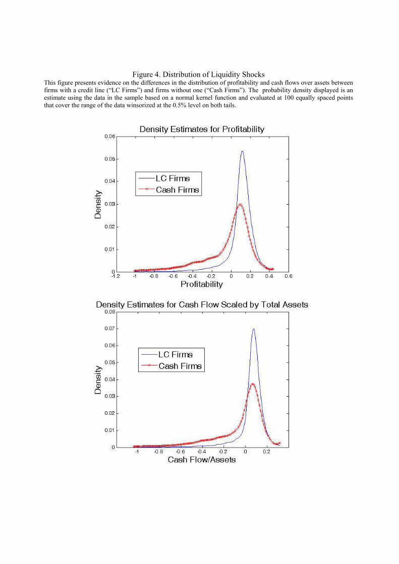
Figure 4. Distribution of Liquidity Shocks This figure presents evidence on the differences in the distribution of profitability and cash flows over assets between firms with a credit line (“LC Firms”) and firms without one (“Cash Firms”). The probability density displayed is an estimate using the data in the sample based on a normal kernel function and evaluated at 100 equally spaced points that cover the range of the data winsorized at the 0.5% level on both tails.

Table 1. Comparison of Firms with and without Credit Lines This table provides summary statistics for the entire sample and for the restricted samples of firms with and without a credit line. The entire sample consists of non-utilities (excluding SIC codes 4900-4949) and non-financials (excluding SIC codes 6000-6999) U.S. firms covered by both Capital IQ and Compustat from 2002 to 2011. We have removed firm- years with 1) negative revenues, and 2) negative or missing assets. After the above filters, the sample consists of 32,671 firm-year observations involving 4,741 unique firms. In this table, “size” is measured as the book value of assets. All variables are winsorized at the 0.5% in both tails of the distribution. The last two columns test for differences between samples with and without undrawn credit using the unequal variances t-test and the two-sample Wilcoxon rank-sum (Mann-Whitney) test. (1) (2) (3) (4) (5) Entire Sample Sample of

Firms with a Credit Line

Sample of Firms without a

Credit Line

Test of Difference with vs. without a Credit Line

Mean [Median]

Mean [Median]

Mean [Median]

t-test p-value

MW p-value

Cash/ Net At 0.657

[0.147] 0.350

[0.094] 1.517

[0.576] 45.658 (0.000)

80.044 (0.000)

Credit Lines/Net At 0.106 [0.071]

0.156 [0.124]

Cash/ Net At (market value)

0.115 [0.054]

0.093 [0.043]

0.185 [0.100]

33.527 (0.000)

50.649 (0.000)

Credit Lines/Net At (market value)

0.067 [0.041]

0.096 [0.071]

Profitability 0.059 [0.107]

0.097 [0.119]

-0.048 [0.045]

-46.411 (0.000)

-52.245 (0.000)

Size 2181.0 [317.2]

2618.9 [453.8]

952.8 [118.5]

-30.560 (0.000)

-55.191 (0.000)

Book Leverage 0.211 [0.152]

0.232 [0.192]

0.151 [0.017]

-30.678 (0.000)

-49.071 (0.000)

M/B 1.728 [1.232]

1.576 [1.152]

2.195 [1.582]

28.841 (0.000)

32.753 (0.000)

Tangibility 0.248 [0.167]

0.273 [0.197]

0.177 [0.094]

-39.567 (0.000)

-47.168 (0.000)

NWC/At 0.050 [0.042]

0.076 [0.064]

-0.019 [-0.015]

-43.110 (0.000)

-44.129 (0.000)

Capex/At 0.054 [0.033]

0.057 [0.036]

0.045 [0.023]

-16.503 (0.000)

-32.671 (0.000)

R&D/Sales 0.370 [0.005]

0.136 [0.000]

1.034 [0.106]

29.731 (0.000)

63.398 (0.000)

Dividend Payer 0.275 [0.000]

0.330 [0.000]

0.117 [0.000]

-49.989 (0.000)

-40.888 (0.000)

Beta KMV 1.245 [1.099]

1.176 [1.054]

1.419 [1.247]

13.428 (0.000)

12.227 (0.000)

Rating Dummy 0.265 [0.000]

0.327 [0.000]

0.092 [0.000]

-59.701 (0.000)

-46.715 (0.000)

Observations 32671 22186 10485

Table 2. The Effect of the GM-Ford Crisis on Liquidity Components This table presents estimates of how the difference in average cash-to-total-liquidity ratios between “treated” and “control” firms changed in the GM-Ford downgrade event period (the “Crisis Period”) relative to the preceding period, which ranges from June 2003 until the start of the crisis. The crisis period is defined as the period that goes from December 2004 to May 2005 (columns 1-3). In columns 4-6 we provide a robustness check using a placebo crisis (December 2003 to May 2004), and in which the preceding period starts in June 2002. In the main test we include only firm-years for which reporting occurred during any month of the fiscal years 2003-2004. We require all firms to have data for the fiscal years 2003-2005. In columns 1 and 4, the treatment group includes firms with a rating (B- or better) in 2003 and 2002 respectively. In columns 2 and 5, the treatment group includes firms with a rating (B- or better) in 2003 and 2002 respectively and with senior and subordinated bonds representing more than 50% of debt. In columns 3 and 6, the treatment group includes firms with a rating (B- or better) in 2003 and 2002 respectively and with senior and subordinated bonds representing more than 70% of debt.

Variable: Cash / (Cash + Credit Lines) GM-Ford Crisis

December 2004-May 2005 Placebo Crisis

December 2003-May 2004 (1) (2) (3) (4) (5) (6)

Rated 2003 Rated 2003 with bonds

>50% of debt

Rated 2003 with bonds

>70% of debt

Rated 2002 Rated 2002 with bonds

>50% of debt

Rated 2002 with bonds >70% of

debt Crisis Dummy -0.012 -0.021*** -0.019*** -0.047*** -0.053*** -0.056*** (0.008) (0.008) (0.007) (0.007) (0.007) (0.007) Treatment Dummy -0.039** -0.051*** -0.049*** -0.013 -0.021 -0.026 (0.018) (0.018) (0.018) (0.018) (0.018) (0.018) Treatment*Crisis 0.022* 0.065*** 0.071*** -0.018 0.001 0.022

(0.013) (0.015) (0.015) (0.013) (0.015) (0.016) Profitability -0.061* -0.059* -0.060* -0.061** -0.061* -0.060* (0.034) (0.034) (0.034) (0.031) (0.031) (0.031) Size -0.014*** -0.014*** -0.014*** -0.017*** -0.016*** -0.017*** (0.004) (0.004) (0.004) (0.004) (0.004) (0.004) Book Leverage -0.365*** -0.363*** -0.362*** -0.339*** -0.339*** -0.337*** (0.033) (0.033) (0.033) (0.031) (0.031) (0.031) M/B 0.023*** 0.023*** 0.023*** 0.019*** 0.019*** 0.020*** (0.003) (0.003) (0.003) (0.003) (0.003) (0.003) Tangibility -0.208*** -0.211*** -0.210*** -0.210*** -0.210*** -0.211*** (0.038) (0.038) (0.038) (0.037) (0.037) (0.037) NWC/Assets -0.659*** -0.659*** -0.659*** -0.514*** -0.514*** -0.514*** (0.034) (0.034) (0.034) (0.033) (0.033) (0.033) Capex/Assets -0.192 -0.190 -0.195 -0.072 -0.073 -0.071 (0.128) (0.128) (0.128) (0.133) (0.133) (0.133) R&D/Sales -0.001 -0.001 -0.001 0.000 0.000 0.000 (0.001) (0.001) (0.001) (0.001) (0.001) (0.001) Dividend Payer -0.055*** -0.056*** -0.057*** -0.048*** -0.048*** -0.049*** (0.013) (0.013) (0.013) (0.014) (0.014) (0.014) CF Volatility -0.035 -0.044 -0.043 -0.095 -0.093 -0.094 (0.184) (0.184) (0.184) (0.163) (0.163) (0.163) Beta KMV 0.023*** 0.024*** 0.023*** 0.020*** 0.020*** 0.019*** (0.003) (0.003) (0.003) (0.003) (0.003) (0.003) Ind. Mean Cash Ratio 0.393*** 0.391*** 0.391*** 0.361*** 0.362*** 0.361***

(0.043) (0.043) (0.043) (0.043) (0.043) (0.043) Observations 4,705 4,705 4,705 4,775 4,775 4,775 R-squared 0.444 0.445 0.446 0.357 0.357 0.357

Table 3. Cash vs. Credit Line Margins over the GM-Ford Crisis This table examines the cash and credit line margins during the GM-Ford downgrade crisis. The crisis period is defined as the period that goes from December 2004 to May 2005. We include only firm-years for which reporting occurred during any month of the fiscal years 2002-2004, or in June 2005. We require all firms to have data for the fiscal years 2003-2005. In columns 1 and 4, the treatment group includes firms with a rating (B- or better) in 2003. In columns 2 and 5, the treatment group includes firms with a rating (B- or better) in 2003 and with senior and subordinated bonds representing more than 50% of debt. In columns 3 and 6, the treatment group includes firms with a rating (B- or better) in 2003 and with senior and subordinated bonds representing more than 70% of debt.

Cash / Net Assets Credit Lines/ Net Assets GM-Ford Crisis

December 2004-May 2005 GM-Ford Crisis

December 2004-May 2005 (1) (2) (3) (4) (5) (6)

Rated 2003 Rated 2003 with bonds

>50% of debt

Rated 2003 with bonds

>70% of debt

Rated 2003 Rated 2003 with bonds

>50% of debt

Rated 2003 with bonds

>70% of debt Crisis Dummy -0.021*** -0.023*** -0.022*** -0.001 -0.001 -0.002 (0.004) (0.004) (0.004) (0.003) (0.003) (0.003) Treatment Dummy -0.001 -0.004 -0.002 0.009 0.009 0.008 (0.006) (0.006) (0.006) (0.006) (0.006) (0.006) Treatment*Crisis 0.015*** 0.025*** 0.026*** -0.010* -0.010** -0.007

(0.005) (0.005) (0.005) (0.005) (0.005) (0.006) Profitability 0.007 0.008 0.007 0.080*** 0.080*** 0.080*** (0.023) (0.023) (0.023) (0.014) (0.014) (0.014) Size -0.015*** -0.015*** -0.015*** -0.001 -0.001 -0.001 (0.002) (0.002) (0.002) (0.001) (0.001) (0.001) Book Leverage -0.144*** -0.144*** -0.143*** 0.037*** 0.037*** 0.037*** (0.014) (0.014) (0.014) (0.011) (0.011) (0.011) M/B 0.021*** 0.021*** 0.021*** -0.001 -0.001 -0.001 (0.002) (0.002) (0.002) (0.001) (0.001) (0.001) Tangibility -0.156*** -0.157*** -0.157*** -0.013 -0.013 -0.013 (0.013) (0.013) (0.013) (0.012) (0.012) (0.012) NWC/Assets -0.222*** -0.222*** -0.222*** 0.173*** 0.173*** 0.173*** (0.015) (0.015) (0.015) (0.014) (0.014) (0.014) Capex/Assets -0.064 -0.064 -0.066 0.082* 0.083* 0.083* (0.049) (0.049) (0.049) (0.046) (0.046) (0.046) R&D/Sales 0.000 0.000 0.000 0.000 0.000 0.000 (0.001) (0.001) (0.001) (0.000) (0.000) (0.000) Dividend Payer -0.007* -0.008* -0.008* 0.027*** 0.027*** 0.027*** (0.004) (0.004) (0.004) (0.005) (0.005) (0.005) CF Volatility 0.571*** 0.568*** 0.569*** 0.236*** 0.237*** 0.236*** (0.114) (0.114) (0.114) (0.082) (0.083) (0.083) Beta KMV 0.004*** 0.004*** 0.004*** -0.004*** -0.004*** -0.004*** (0.002) (0.002) (0.002) (0.001) (0.001) (0.001) Ind. Mean Cash Ratio 0.041*** 0.040*** 0.040*** -0.080*** -0.079*** -0.079***

(0.015) (0.015) (0.015) (0.015) (0.015) (0.015) Observations 4,689 4,689 4,689 4,707 4,707 4,707 R-squared 0.429 0.430 0.430 0.194 0.194 0.193

Table 4. Credit Line Usage across Top and Bottom Quintiles of Hedging Needs This table provides summary statistics across groups of high versus low correlation of investment opportunities and cash-flow (low and high hedging needs, respectively). Hedging needs are calculated at the 3-digit SIC code industry level as the correlation between firm-level cash flow and the mean industry annual investment activities (Hedging Investment Activities, item 311 + 46), and the median industry Tobin’s Q (Hedging Tobin’s Q). High (low) hedging needs firms are those with a correlation in the bottom (top) quintile. Total liquidity is cash and short-term investments plus undrawn credit. In Panel A we examine the relationship between hedging needs and liquidity variables. In Panel B we examine the relationship between hedging needs and the residuals of regressions in which the dependent variables are the liquidity variables and in which we control for the following firm characteristics: profitability, size, book leverage, M/B, tangibility, NWC/assets, capex/assets, R&D/sales, dividend payer dummy, CF volatility, beta KMV, and rating. In both panels we include a test for differences between samples with high and low hedging needs using the unequal variances t-test.

Panel A Variable: Mean (Median)

Presence of a Credit Line (Dummy)

Undrawn Credit / Net Assets

Undrawn Credit / Total Liquidity

Revolving Credit /Net Assets

Industry median Invest. Activities

High hedging needs 0.573 0.082 0.267 0.022

N= 6288   (1.000) (0.029) (0.109) (0.000)

Low hedging needs 0.848 0.127 0.536 0.042

N= 6568   (1.000) (0.105) (0.587) (0.000)

t-test 35.919 21.081 46.402 16.362

(p-value) (0.000) (0.000) (0.000) (0.000)

Industry median Tobin’s Q

High hedging needs 0.595 0.087 0.289 0.021

N= 6488   (1.000) (0.037) (0.151) (0.000)

Low hedging needs 0.831 0.133 0.544 0.054

N=6657 (1.000) (0.107) (0.616) (0.000)

t-test 30.821 20.761 42.933 24.063

(p-value) (0.000) (0.000) (0.000) (0.000)

Panel B Residuals: Mean (Median)

Presence of a Credit Line (Dummy)

Undrawn Credit / Net Assets

Undrawn Credit / Total Liquidity

Revolving Credit /Net Assets

Industry median Invest. Activities

High hedging needs 0.056 0.006 0.250 0.022

N= 6288   (0.366) (-0.024) (0.088) (0.000)

Low hedging needs 0.244 0.022 0.512 0.042

N= 6568   (0.389) (0.000) (0.554) (0.000)

t-test 9.839 6.765 45.716 16.362

(p-value) (0.000) (0.000) (0.000) (0.000)

Industry median Tobin’s Q

High hedging needs 0.055 0.009 0.271 0.021

N= 6488 (0.360) (-0.020) (0.117) (0.000)

Low hedging needs 0.226 0.030 0.526 0.054

N=6657 (0.369) (0.004) (0.587) (0.000)

t-test 9.058 8.479 43.387 24.063

(p-value) (0.000) (0.000) (0.000) (0.000)

Table 5. Hedging Needs and Covenants on Credit Lines This table estimates the relationship between hedging needs and the use of covenants on credit lines using a Poisson specification. Hedging needs are calculated at the 3-digit SIC code industry level as the correlation between firm-level cash flow and the mean industry annual investment activities (Hedging Investment Activities, item 311 + 46), and the median industry Tobin’s Q (Hedging Tobin’s Q). We obtain data on covenants from LPC Dealscan. We list all the covenants attached to credit lines for the firms in our sample during the period 2002-2008. In most cases, firms are granted several new credit line facilities in the same year. For these cases we report the median number of covenant across facilities. General Purpose LC is a dummy that takes value 1 if the stated purpose of the line of credit is “General Corporate Purposes”, as reported in LPC Dealscan. When firms are granted several new credit line facilities in the same year we report the median value. All regressions include year fixed effects. Robust standard errors clustered at the firm level are reported in parentheses. ***, **, and * denote statistical significance at the 1%, 5%, and 10% levels, respectively. (1) (2) (3) (4) (5) (6) (7) (8)

Covenant Index Covenant Index Covenant Index Covenant Index

Drucker and Puri (2010) Demiroglu and James (2010) Only CF Covenants Only Sweeps

Hedging Inv. Activities -0.274*** -0.168* -0.742*** -0.407*** (0.082) (0.094) (0.130) (0.146)

Hedging Tobin’s Q -0.232*** -0.069 -0.602*** -0.505*** (0.076) (0.087) (0.124) (0.139)

Profitability 0.224** 0.219* -0.146 -0.158 0.264 0.244 -0.256 -0.247 (0.112) (0.112) (0.122) (0.122) (0.177) (0.177) (0.196) (0.197)

Size -0.238*** -0.240*** -0.242*** -0.243*** -0.273*** -0.277*** -0.361*** -0.362*** (0.008) (0.008) (0.010) (0.010) (0.013) (0.013) (0.015) (0.015)

Book Leverage 0.716*** 0.718*** 0.737*** 0.740*** 0.774*** 0.778*** 1.418*** 1.415*** (0.046) (0.046) (0.053) (0.053) (0.071) (0.071) (0.075) (0.075)

MB -0.103*** -0.101*** -0.138*** -0.136*** -0.108*** -0.103*** -0.201*** -0.200*** (0.012) (0.012) (0.014) (0.014) (0.019) (0.019) (0.024) (0.024)

Rated 0.146*** 0.147*** 0.128*** 0.127*** 0.117*** 0.120*** 0.339*** 0.346*** (0.026) (0.027) (0.030) (0.030) (0.042) (0.042) (0.047) (0.047)

CF Volatility -1.906*** -1.873*** -1.419** -1.416** -1.661* -1.587* -1.741 -1.670 (0.590) (0.590) (0.650) (0.651) (0.913) (0.913) (1.069) (1.068)

General Purpose LC -0.225*** -0.226*** -0.249*** -0.250*** -0.212*** -0.214*** -0.394*** -0.395*** (0.020) (0.020) (0.023) (0.023) (0.032) (0.032) (0.035) (0.035)

Ln(Maturity) of LC 0.407*** 0.407*** 0.476*** 0.476*** 0.469*** 0.469*** 0.751*** 0.750*** (0.022) (0.022) (0.026) (0.026) (0.036) (0.036) (0.045) (0.045)

Facility Amount/At -0.629*** -0.628*** -0.241*** -0.249*** -0.864*** -0.868*** -1.330*** -1.308*** (0.073) (0.073) (0.080) (0.080) (0.116) (0.117) (0.136) (0.136)

Observations 4,637 4,637 4,637 4,637 4,637 4,637 4,637 4,637 Pseudo R2 0.098 0.098 0.101 0.101 0.084 0.083 0.139 0.139

Table 6. Revocations and Drawdowns This table presents Probit (marginal effects dF/dx) and OLS regression results for the contemporaneous relationship between restriction of access to credit lines, profitability and hedging needs (columns 1-4), and for the relationship between drawdown of credit lines, profitability and hedging needs (columns 5-6). In columns 1-2 the dependent variable is a dummy for a full revocation of the credit line. In columns 3-4 the dependent variable is a dummy for a decrease in undrawn credit greater than 50% of the outstanding amount. In columns 5-6 the dependent variable is the annual change in drawn credit lines as a percentage of total assets. Hedging needs are calculated at the 3-digit SIC code industry level as the correlation between firm-level cash flow and the mean industry annual investment activities (Hedging Investment Activities, item 311 + 46), and the median industry Tobin’s Q (Hedging Tobin’s Q). Year, Rating and Exchange fixed effects included. Rating fixed effects are based on 22 rating dummies and the unrated dummy. Robust standard errors clustered at the firm level are reported in parentheses. ***, **, and * denote statistical significance at the 1%, 5%, and 10% levels. All regressions include a constant term (unreported).

(1) (2) (3) (4) (5) (6) Full Revocation

of Credit Line (Dummy)

Full or Partial (>50%) Revocation of Credit Line

(Dummy)

Drawdown of Credit Lines

Hedging Inv Act -0.023** -0.034* -0.001 (0.011) (0.019) (0.004) Hedging Tobin’s Q -0.040*** -0.027 0.009*** (0.012) (0.018) (0.004) Profitability -0.050*** -0.048*** -0.112*** -0.110*** -0.024*** -0.024*** (0.010) (0.010) (0.018) (0.018) (0.007) (0.007) Size -0.001 -0.001 -0.002 -0.002 0.001 0.001 (0.001) (0.001) (0.002) (0.002) (0.000) (0.000) Book Leverage -0.037*** -0.036*** -0.047*** -0.048*** 0.046*** 0.046*** (0.008) (0.008) (0.013) (0.013) (0.005) (0.005) M/B 0.003*** 0.003*** 0.003* 0.003* -0.001* -0.001 (0.001) (0.001) (0.002) (0.002) (0.001) (0.001) Tangibility -0.017** -0.017** -0.003 -0.006 -0.025*** -0.027*** (0.009) (0.009) (0.014) (0.013) (0.004) (0.004) NWC/Assets -0.070*** -0.067*** -0.141*** -0.143*** -0.004 -0.006 (0.008) (0.008) (0.014) (0.014) (0.004) (0.004) Capex/Assets -0.039 -0.033 -0.235*** -0.232*** 0.176*** 0.176*** (0.032) (0.031) (0.054) (0.054) (0.020) (0.020) R&D/Sales 0.001 0.001 -0.002 -0.001 -0.002 -0.002 (0.002) (0.002) (0.003) (0.003) (0.001) (0.001) Div. Payer Dummy -0.014*** -0.014*** -0.019*** -0.020*** 0.005*** 0.005*** (0.003) (0.003) (0.005) (0.005) (0.001) (0.001) CF Volatility 0.064 0.072 0.341*** 0.347*** -0.239*** -0.243*** (0.053) (0.053) (0.087) (0.087) (0.031) (0.032) Beta KMV 0.002* 0.002* 0.002 0.002 0.000 0.000 (0.001) (0.001) (0.002) (0.002) (0.001) (0.001) Observations 15,116 15,116 15,129 15,129 15,176 15,176 R-squared 0.141 0.143 0.0930 0.0928 0.059 0.059

Table 7. Probability of a Liquidity Event This table examines the probability of a drawdown in credit lines or a reduction in cash associated with a drop in profitability. In Panel A, we compute the probability of profitability falling below 0% and 5%, respectively for firms with and without a credit line. In Panel B, we define liquidity events as follows: for credit line drawdowns, a liquidity event occurs if there is an increase in drawn revolving credit (ΔRC>0) while profitability is negative; for cash, a liquidity event occurs if there is a reduction in cash (ΔCash and ST Investments<0) while profitability is negative. The probability of a liquidity event for credit lines is computed as the ratio of credit line liquidity events divided by the number of firm-years with a credit line. The probability of a liquidity event for cash is computed as the ratio of cash liquidity events divided by the number of firm years without a credit line. Panel A: Probability of a negative cash flow shock

With Credit Line

W/out Credit Line t-stat p-value wilcoxon p-value

Probability of Profits < 0% 0.128 0.368 52.644 (0.000) 59.627 (0.000)

Probability of Profits < 5% 0.203 0.476 55.001 (0.000) 58.113 (0.000)

Panel B: Probability of a liquidity event

Credit Line Cash t-stat p-value wilcoxon p-value

Probability of a Liquidity Event 0.016 0.185 40.494 (0.000) 58.691 (0.000)

Probability of a Liquidity Event > 0.5% of Assets 0.014 0.179 39.726 (0.000) 57.833 (0.000)

Tables for the Appendix

Table A1. Access to Credit Lines This table relates firm characteristics to various liquidity measures. In column (1) and (2) we run Probit regressions (marginal effects dF/dx) for the presence of a credit line, where the dependent variable is a dummy that takes value one, if the firm has an undrawn credit line. Column (1) is for all the firms in the sample, while column (2) is for the sub-sample of rated firms (>CCC). In columns (3) and (4) we run OLS regressions for cash and short-term investments as a percentage of total liquidity. Total liquidity is computed as cash and short-term investments plus undrawn credit. Column (3) is for sub-sample of rated firms (>CCC), while column (4) is for the sub-sample of rated firms that have a credit line. In column (5) we run an OLS regression for cash and short-term investments as a percentage of total assets, on the sub-sample of rated firms (>CCC) with a credit line. Year and Exchange fixed effects included. Robust standard errors clustered at the firm level are reported in parentheses. ***, **, and * denote statistical significance at the 1%, 5%, and 10% levels, respectively.

(1) (2) (3) (4) (5) Presence of a Credit Line

(Dummy) Cash/

Total Liquidity Cash/

Net Assets All Firms Rated Rated Rated with a LC Rated with a LC Profitability 0.362*** 0.116* -0.190** 0.041 -0.078 (0.041) (0.069) (0.086) (0.087) (0.080) Size 0.002 -0.013** 0.048*** 0.041*** -0.003 (0.005) (0.006) (0.007) (0.007) (0.004) Book Leverage 0.271*** 0.080*** -0.338*** -0.314*** -0.202*** (0.034) (0.028) (0.037) (0.035) (0.032) M/B -0.035*** -0.029*** 0.082*** 0.055*** 0.061*** (0.005) (0.006) (0.009) (0.009) (0.011) Tangibility 0.201*** 0.043 -0.156*** -0.093*** -0.119*** (0.039) (0.032) (0.038) (0.034) (0.018) NWC/Assets 0.504*** 0.134*** -0.430*** -0.410*** -0.286*** (0.036) (0.043) (0.056) (0.053) (0.036) Capex/Assets 0.210* 0.015 -0.553*** -0.637*** -0.126*** (0.126) (0.123) (0.137) (0.115) (0.043) R&D/Sales -0.023** -0.304*** 0.037* 0.878*** 0.555*** (0.009) (0.084) (0.022) (0.155) (0.159) Div. Payer Dum. 0.076*** 0.015 -0.071*** -0.058*** -0.006 (0.015) (0.011) (0.015) (0.014) (0.008) CF Volatility -2.172*** -0.977** 3.591*** 2.948*** 1.059*** (0.555) (0.382) (0.537) (0.596) (0.323) Beta KMV -0.004 0.002 0.029*** 0.031*** 0.017*** (0.003) (0.004) (0.005) (0.005) (0.003) Rating -0.009*** -0.012*** 0.019*** 0.017*** 0.008*** (0.001) (0.003) (0.004) (0.003) (0.002) Observations 23,653 6,848 6,839 6,166 6,172 R-squared 0.272 0.259 0.287 0.286 0.239

Table A2. Robustness Tests on GM-Ford Crisis This table presents two robustness checks for our tests on the GM-Ford crisis (Table 2). In column 1-3 we sort firms conditional on having a rating in 2002 (rather than 2003 as in the main table). In columns 4-6 we include June 2005 in the crisis period.

Variable: Cash / (Cash + Undrawn) Sorting in 2002

December 2004-May 2005 Alternative Definition of Crisis

December 2004-June 2005 (1) (2) (3) (4) (5) (6)

Rated 2002 Rated 2002 with bonds

>50% of debt

Rated 2002 with bonds

>70% of debt

Rated 2003 Rated 2003 with bonds

>50% of debt

Rated 2003 with bonds

>70% of debt Crisis Dummy -0.012 -0.020*** -0.018** -0.015** -0.024*** -0.022*** (0.008) (0.007) (0.007) (0.007) (0.007) (0.006) Treatment Dummy -0.041** -0.052*** -0.050*** -0.041** -0.053*** -0.051*** (0.018) (0.018) (0.018) (0.018) (0.018) (0.018) Treatment*Crisis 0.024* 0.065*** 0.069*** 0.024** 0.065*** 0.072***

(0.013) (0.015) (0.016) (0.011) (0.014) (0.015) Profitability -0.061* -0.059* -0.060* -0.061* -0.060* -0.060* (0.034) (0.034) (0.034) (0.034) (0.034) (0.034) Size -0.014*** -0.014*** -0.014*** -0.014*** -0.014*** -0.014*** (0.004) (0.004) (0.004) (0.004) (0.004) (0.004) Book Leverage -0.365*** -0.364*** -0.363*** -0.365*** -0.363*** -0.361*** (0.033) (0.033) (0.033) (0.033) (0.033) (0.033) M/B 0.023*** 0.023*** 0.023*** 0.023*** 0.023*** 0.023*** (0.003) (0.003) (0.003) (0.003) (0.003) (0.003) Tangibility -0.206*** -0.209*** -0.208*** -0.209*** -0.212*** -0.211*** (0.038) (0.038) (0.038) (0.038) (0.038) (0.038) NWC/Assets -0.660*** -0.660*** -0.660*** -0.659*** -0.659*** -0.659*** (0.034) (0.034) (0.034) (0.034) (0.034) (0.034) Capex/Assets -0.198 -0.194 -0.201 -0.188 -0.185 -0.190 (0.128) (0.128) (0.128) (0.128) (0.128) (0.128) R&D/Sales -0.001 -0.001 -0.001 -0.001 -0.001 -0.001 (0.001) (0.001) (0.001) (0.001) (0.001) (0.001) Dividend Payer -0.055*** -0.056*** -0.056*** -0.055*** -0.056*** -0.056*** (0.013) (0.013) (0.013) (0.013) (0.013) (0.013) CF Volatility -0.031 -0.040 -0.039 -0.042 -0.052 -0.052 (0.184) (0.184) (0.184) (0.184) (0.184) (0.184) Beta KMV 0.023*** 0.024*** 0.023*** 0.023*** 0.024*** 0.024*** (0.003) (0.003) (0.003) (0.003) (0.003) (0.003) Ind. Mean Cash Ratio 0.394*** 0.393*** 0.393*** 0.393*** 0.392*** 0.392***

(0.043) (0.043) (0.043) (0.043) (0.043) (0.043) Observations 4,705 4,705 4,705 4,705 4,705 4,705 R-squared 0.444 0.445 0.445 0.444 0.445 0.446

Table A3. Exogeneity Checks on the GM-Ford Event This table examines possible liquidity shocks associated with the GM-Ford downgrade. Columns 1-3 examine the restriction of access to credit lines in association with the GM-Ford event. Columns 4-6 examine covenant violations associated with the GM-Ford event. The crisis period is defined as the period that goes from December 2004 to May 2005. We include only firm-years for which reporting occurred during any month of the fiscal years 2002-2004, or in June 2005. We require all firms to have data for the fiscal years 2003-2005 and to have an outstanding credit line. Depending on the column, the treatment group includes firms with a rating (B- or better) in 2003 and with senior and subordinated bonds representing more than 50% or 70% of debt. Robust standard errors clustered at the firm level are reported in parentheses. ***, **, and * denote statistical significance at the 1%, 5%, and 10% levels. All regressions include a constant term (unreported). (1) (2) (3) (4) (5) (6)

Revocation of Credit Line (Dummy)

Covenant Violation (Dummy)

Rated 2003 Rated 2003 with bonds

>50% of debt

Rated 2003 with bonds

>70% of debt

Rated 2003 Rated 2003 with bonds

>50% of debt

Rated 2003 with bonds

>70% of debt

Crisis Dummy 0.063 0.062 0.074 0.068 0.034 0.008 (0.158) (0.152) (0.150) (0.118) (0.107) (0.105) Treatment Dummy -0.364 -0.374 -0.282 -0.134 -0.252 -0.345** (0.418) (0.321) (0.270) (0.214) (0.165) (0.152) Treatment*Crisis 0.182 0.246 0.125 -0.321 -0.218 -0.076

(0.436) (0.337) (0.308) (0.230) (0.189) (0.181) Profitability 0.254 0.263 0.257 -1.904*** -1.909*** -1.905*** (0.373) (0.371) (0.373) (0.467) (0.468) (0.470) Size -0.064 -0.065 -0.064 -0.068* -0.065* -0.066* (0.058) (0.058) (0.058) (0.036) (0.036) (0.036) Book Leverage -0.168 -0.168 -0.161 1.361*** 1.351*** 1.352*** (0.478) (0.480) (0.479) (0.242) (0.241) (0.241) M/B 0.029 0.029 0.029 -0.367*** -0.367*** -0.367*** (0.036) (0.036) (0.036) (0.066) (0.066) (0.067) Tangibility -0.486 -0.500 -0.482 -0.086 -0.068 -0.083 (0.637) (0.637) (0.636) (0.305) (0.305) (0.303) NWC/Assets -1.877*** -1.883*** -1.881*** -0.351 -0.347 -0.353 (0.435) (0.436) (0.435) (0.304) (0.305) (0.305) Capex/Assets 0.464 0.453 0.437 0.113 0.087 0.086 (2.002) (2.006) (1.999) (1.046) (1.041) (1.042) R&D/Sales -0.025 -0.024 -0.025 -1.141 -1.092 -1.106 (0.017) (0.017) (0.018) (0.800) (0.785) (0.790) Dividend Payer -0.321* -0.325* -0.322* -0.227** -0.228** -0.229** (0.188) (0.187) (0.187) (0.106) (0.106) (0.106) CF Volatility 1.193 1.210 1.190 7.514*** 7.580*** 7.558*** (2.818) (2.814) (2.816) (2.338) (2.339) (2.344) Beta KMV 0.141*** 0.141*** 0.140*** -0.022 -0.021 -0.020 (0.046) (0.047) (0.046) (0.035) (0.035) (0.035) Ind. Mean Cash Ratio 1.633*** 1.621*** 1.633*** 0.471 0.452 0.449

(0.518) (0.516) (0.520) (0.326) (0.325) (0.324) Observations 1,803 1,803 1,803 1,803 1,803 1,803(Pseudo) R-2 0.211 0.211 0.211 0.172 0.171 0.171

Description of Variables Variable Construction Beta KMV Firm's asset (unlevered) beta, calculated from equity (levered) betas and a Merton-KMV formula as in Acharya,

Almeida and Campello (2010) Book Leverage Total Debt / Total Assets (6) BV Equity Total Assets (6) – Total Liabilities (181) – Deferred Taxes and Investment Tax Credit (35) – Preferred Stock Capex/Assets Capital Expenditures (128)/ Total Assets (6) Cash Flow/Assets (Operating Income Before Depreciation (13) – Interest Expense (15) – Income Taxes (16) – Dividends (21)) / Total

Assets (6) Cash Ratio Cash and Short-Term Investments (1) / (Cash and Short-Term Investments (1) +(Undrawn) Credit Lines (CapitalIQ)) Cash/Net Assets Cash and Short-Term Investments (1) / Net Assets Cash/Net Assets (market value)

Cash and Short-Term Investments (1) / (Total Assets (6)- BV Equity + Market Value of Equity - Cash and Short-Term Investments (1))

CF Volatility Standard Deviation of Operating Income Before Depreciation (13) over Previous 12 Quarters Scaled by Total Assets (6)

Covenant Index (Demiroglu and James (2010))

Sum of the following covenants: Collateral Release, Dividend Restrictions, Dummy Financial Covenants, Asset Sales Sweep, Equity Issuance Sweep, Debt Issuance Sweep. Where Dummy Financial Covenants equals one is at least two of the following covenants are included: Debt/Tangible Assets, Max Capex, Max Debt/Assets, Max Debt/Ebitda, Max Debt/Equity, Max Leverage, Max Senior Debt/Ebitda, Max Senior Leverage, Min Change Interest Coverage, Min Current Ratio, Min Debt Coverage, Min Ebitda, Min Equity/Asset, Min Fixed Charge, Min Interest Coverage, Min Net Worth/Assets, Min Quick Ratio, Net Worth, Other Ratio, Other, Tangible Net Worth.

Covenant Index (Drucker and Puri (2010)

Sum of following covenants: % Of Excess CF, % Of Net Income, Asset Sales Sweep, Collateral Release, Debt Issuance Sweep, Dividend Restrictions, Equity Issuance Sweep, Excess CF Sweep, Insurance Proceeds Sweep, Max Capex , Max Debt/Assets, Max Debt/Ebitda, Max Debt/Equity, Max Debt/Tangible Assets, Max Leverage, Max Senior Debt/Ebitda, Max Senior Leverage, Min Change Interest Coverage, Min Current Ratio, Min Debt Coverage, Min Ebitda, Min Equity/Asset, Min Fixed Charge, Min Interest Coverage, Min Net Worth/Assets, Min Quick Ratio, Net Worth, Other, Other Ratio, Tangible Net Worth.

Covenant Index (Only CF Covenants)

Sum of following covenants: % Of Excess CF, % Of Net Income, Excess CF Sweep, Max Capex, Max Debt/Ebitda, Max Senior Debt/Ebitda, Min Change Interest Coverage, Min Ebitda.

Covenant Index (Only Sweeps)

Sum of following covenants: Asset Sales Sweep, Debt Issuance Sweep, Equity Issuance Sweep, Excess CF Sweep, Insurance Proceeds Sweep.

Credit Lines/Net Assets (Undrawn) Credit Lines (CapitalIQ)/ Net Assets Credit Lines/Net Assets (market value)

(Undrawn) Credit Lines (CapitalIQ) / (Total Assets (6)- BV Equity + Market Value of Equity - Cash and Short-Term Investments (1))

Dividend Payer Dummy A dummy variable that takes the value of one if common stock dividends (21) are positive, and zero otherwise Full (Partial) Revocation of Credit Line (Dummy)

Takes value 1 in period t if a firm has available undrawn credit in t-1 and no available undrawn credit in t, and drawn credit has not increased between t-1 and t. Partial revocations are those in which undrawn credit availability decreases by 30% or more.

Hedging based on investment Activities

Correlation between three-digit median industry investment activities adjusted for R&D expenses (item 311 + 46) and the firm-year cash flows measured as in Acharya, Almeida and Campello (2007). The three-digit median industry investment activities is computed on the sample of unconstrained firms, defined as firms that pay dividends, have assets above $500m and rating above B+.

Hedging based on Tobin’s Q

Correlation between three-digit median industry market-to-book and the firm-year cash flows measured as in Acharya, Almeida and Campello (2007). The three-digit median industry market-to-book is computed on the sample of unconstrained firms, defined as firms that pay dividends, have assets above $500m and rating above B+.

Industry Mean Cash Ratio

Mean cash ratio at the two digit SIC code

M/B (Market Value of Equity + Total Debt + Preferred Stock Liquidating Value (10) – Deferred Taxes and Investment Tax Credit (35)) / Total Assets (6)

Market Value of Equity Stock Price (199) × Common Shares Used to Calculate EPS (54) Net Assets Assets (item 6) minus Cash and Short-Term Investments (1) ) NWC/ Assets (Working Capital (179) - Cash and Short-Term Investments (1))/ Total Assets (6) Preferred Stock Max[Preferred Stock Liquidating Value (10), Preferred Stock Redemption Value (56), Preferred Stock Carrying Value

(130)] Profitability Operating Income Before Depreciation (13) / Total Assets (6) R&D/Sales Research and Development Expenses (46) / Sales (12) Rated A dummy variable that takes the value of one if the firm is rated by the S&P, and zero otherwise Rating Monthly S&P ratings (280). Takes 23 values: 1 = "AAA", 2="AA+", 3="AA", 4="AA-", 5="A+", 6="A", 7="A-",

8="BBB+", 9="BBB", 10="BBB-", 11="BB+", 12="BB", 13="BB-", 14="B+", 15="B", 16="B-", 17="CCC+", 18="CCC", 19="CCC-", 20="CC", 21="SD", 22="D", 23= Unrated

Revolving Credit / Net Assets

Revolving Credit (CapitalIQ)/ Net Assets

Size Logarithm of Revenues (12) Tangibility Net Property, Plant, and Equipment (8) / Total Assets (6) Total Debt Debt in Current Liabilities (34) + Long-Term Debt (9)