Electronic copy available at: http://ssrn.com/abstract=1770066

Credit Default Swaps, Firm Financing and the Economy ∗

Murillo Campello

Cornell University and NBER

campello@cornell.edu

Rafael Matta

University of Amsterdam

matta@uva.nl

August 30, 2013

Abstract

This paper develops a model of CDS demand when investment is subject to economic fluctuations

and verification is imperfect. We show that CDS overinsurance (insurance in excess of renegotiation

proceeds) is procyclical and allows for greater financing of firms with positive NPV projects. In bad

times, CDS overinsurance triggers the early liquidation of firms with low continuation values. Our

analysis explains the optimality of CDS contracting and reconciles evidence showing that CDSs are

most beneficial for firms that are safer and have higher continuation values. The model generates a

number of empirical predictions and provides insights on the regulation of CDS markets.

Keywords: CDS, Bankruptcy, Moral Hazard, Financing Efficiency, Regulation.

JEL: G33, D86, D61.

∗We thank Viral Acharya, Heitor Almeida, Ola Bengtsson, Dan Bernhardt, Charlie Calomiris, Diemo Dietrich, ErasmoGiambona, Charlie Kahn, and seminar participants at the University of Illinois for their comments and suggestions.

Electronic copy available at: http://ssrn.com/abstract=1770066

Credit Default Swaps, Firm Financing and the Economy

August 30, 2013

Abstract

This paper develops a model of CDS demand when investment is subject to economic fluctuations

and verification is imperfect. We show that CDS overinsurance (insurance in excess of renegotiation

proceeds) is procyclical and allows for greater financing of firms with positive NPV projects. In bad

times, CDS overinsurance triggers the early liquidation of firms with low continuation values. Our

analysis explains the optimality of CDS contracting and reconciles evidence showing that CDSs are

most beneficial for firms that are safer and have higher continuation values. The model generates a

number of empirical predictions and provides insights on the regulation of CDS markets.

Keywords: CDS, Bankruptcy, Moral Hazard, Financing Efficiency, Regulation.

JEL: G33, D86, D61.

“Some derivatives ought not to be allowed to be traded at all. I have in mind credit default swaps.The more I’ve heard about them, the more I’ve realized they’re truly toxic.”

— George Soros, June 2009.

1 Introduction

The 2000s witnessed a formidable growth in the market for credit default swaps. According to the In-

ternational Swaps and Derivatives Association (ISDA), the outstanding amount of CDS contracts grew

from $3 trillion in 2003 to a peak of $62 trillion in 2007. The 2008–9 crisis brought attention to these

contracts, and there is ongoing debate about whether CDSs contributed to the crisis and how to regulate

CDS markets.1 Surprisingly, however, little is known about why CDSs exist in the first place. We know

little about the role of CDSs in financial markets, what contracting inefficiencies they address, or whether

they affect the availability of credit in the economy. Understanding these issues should strike anyone as

an important step for improving financial architecture and regulation over the next decade.

A CDS is a bilateral agreement between a debt protection seller and a debt protection buyer. The

buyer makes periodic payments to the seller in exchange for compensation in the event a borrower

defaults on its debt. Notably, Hu and Black (2008a,b) argue that CDSs can give rise to the empty

creditor problem. Simply put, lenders protected by CDS might have low incentives to participate in out-

of-court restructurings of distressed firms since formal default triggers immediate compensation for their

exposure. The incentives to engage in restructuring could be even lower if lenders “overinsure;” that is,

their protection payoff surpasses the amount of debt that can be recovered in default. In these cases,

lenders might collect large profits from bankruptcy. CDS-insured lenders might thus force distressed firms

into bankruptcy even when continuation would be optimal.2

The introduction of CDS contracts may alter the dynamics of corporate financing since optimal lend-

ing decisions are influenced by expected distress outcomes. While there is growing interest in the impact

of CDSs on creditor–borrower relations, the literature lacks a model that examines important questions

about these contracts. How do firm characteristics such as risk and size influence CDS contracting?

How do CDSs affect borrowers’ incentives to avoid bankruptcy? How do economic conditions affect the

demand for CDSs? Do CDS markets affect the availability of credit in the economy?

1Title VII of Dodd-Frank Act (HR #4173) gives the SEC regulatory authority over swaps, including CDSs. TheAct requires the reporting of trades, sets position limits, imposes margin requirements, and moves swaps away fromover-the-counter markets into organized exchanges.

2Numerous accounts blame overinsured CDS lenders for blocking out-of-court restructurings of high profile firms duringthe Financial Crisis. In 2009 alone, companies in that category included Six Flags, Harrah’s, GM, Chrysler, Unisys, R. H.Donnelley, Abitibi Bowater, Marconi, and Lyondell Basell.

1

This paper develops a model of CDS contracting when investment is subject to changes in economic

conditions and verification is imperfect. To our knowledge, this is the first study to examine the optimal

demand for CDS in a setting that incorporates these real-world complexities (we discuss the existing

literature shortly). Creditors choose the amount of CDS protection to modulate their economic exposure

to borrowers and our analysis shows how this choice is made, describing its larger economic consequences.

The rich setup in which we analyze CDS contracting in this paper leads to a number of novel empirical

predictions and helps explain reported empirical regularities.

In a nutshell, our model shows that CDS overinsurance is associated with the implementation of

policies that maximize the likelihood that projects succeed and alleviate the empty creditor problem.

Our model also shows that CDS overinsurance is associated with safer firms and is procyclical (more

pronounced in booms). Indeed, our study suggests that CDS contracts may have emerged and become

popular in the early 2000s precisely by virtue of its overinsurance capabilities. It additionally shows

that CDS contracts can boost the availability of credit in the economy. Our paper shows that while

CDSs facilitate borrowing by credit-constrained firms, CDSs will also be associated with their demise in

bad times, leading to the “appearance” that CDSs aggravate the impact of economic downturns. As we

discuss below, proposed regulatory changes that prohibit lenders to overinsure via CDS may have the

adverse consequence of reducing the availability of credit when firms most need it.

Let us provide context to our framework and discuss the implications of our analysis. In credit mar-

kets lenders have to design contracts that account for commitment issues, moral hazard problems, and

inefficient restructuring protocols. Our analysis of CDS contracting incorporates these features. In the

model, borrowers face a limited commitment problem in that they cannot commit to pay out cash flows

from their projects. In effect, borrowers can divert cash flows and strategically trigger debt renegotiation

even when projects succeed. Moreover, the amount of effort that borrowers dedicate to their projects is

unobservable, even though that effort affects cash flows. Finally, we allow for restructuring to be a costly

process that can dissipate enterprise value.

As is standard in contracting problems, lenders can refuse to renegotiate contracts in default and force

firms into liquidation; else they can engage in out-of-court restructurings and bargain over the portion of

firm continuation values that can be verified. In the presence of CDS contracts, however, they have an

alternative course of action: lenders can insure against strategic renegotiation. In essence, CDSs trigger

an insurance payment by a third party if a “credit event” occurs.3 As we demonstrate, the innovation

3As desfined by the ISDA, credit events include default, debt acceleration, failure to pay, repudiation/moratorium, andbankruptcy. The standard CDS contract does not recognize out-of-court restructuring as a credit event.

2

brought about by CDSs is that they can be uniquely used to strengthen lenders’ bargaining position by:

(1) increasing debt repayments when investments succeed and (2) increasing lenders’ share of proceeds

in default states. Differently put, CDSs can be used to modulate whether lenders will have a stronger

bargaining position when projects succeed or when they fail. To describe this tradeoff concretely, let’s

discuss how it works under different degrees of CDS insurance.

If lenders buy CDS protection beyond the maximum amount they can receive in restructurings (i.e.,

lenders “overinsure” or have so-called “negative net economic ownership”), they pre-commit to forcing

defaulting borrowers into bankruptcy. Intuitively, the mechanism works somewhat similarly to standard

insurance. CDSs resemble actuarially fairly-priced policies and overinsurance increases both the like-

lihood that the insured party will require payoffs (immediate compensation for credit events) and the

associated insurance premia (CDS fees).4 Once a credit event happens, the one-time payoff from seeking

immediate borrower liquidation is large enough to commit CDS-protected lenders with that course of

action. As a result, borrowers are prevented from capturing rents from default–continuation strategies.

This not only discourages borrowers from defaulting strategically, but also incentivizes them to exert

high effort, increasing the likelihood that investments succeed. By altering the dynamics of renegotia-

tions and heightening borrowers’ incentives, overinsured lenders maximize regular debt repayments in

good investment states (e.g., extraction of higher “debt coupons”).

If lenders buy an amount of CDS protection that equals the maximum payoff under restructuring

(“zero net economic ownership”), they do not commit to unconditional liquidation in default states.5

Instead, they position themselves so as to bargain over surpluses stemming from out-of-court renegotia-

tions. Although zero net economic ownership maximizes the amount of debt repayment consistent with

no liquidation, it leaves some surplus for borrowers when the verification of funds in default states is

imperfect. Because “just-insured” lenders are relatively less inclined to call for bankruptcy if borrowers

default, they pay lower fees for their CDS insurance. At the same time, because borrowers retain a frac-

tion of restructuring values and know forced liquidation is less likely to happen, they are more prone to

strategically default. This dynamic determines the tradeoffs faced by just-insured lenders. These lenders

forego debt repayment surpluses that are extracted when investments succeed in exchange for higher

renegotiation proceeds when investments fail.

4As in any competitive market, the insurance premium schedule is such that, in expectation, the insured party does notmake an economic profit (e.g., higher insurance payoffs are associated with higher premia).

5For completeness, in the law and economics literature “positive net economic ownership” refers to the case in whichlenders do not completely hedge their economic exposure to borrowers (see Hu and Black (2007)). We will later discusscurrent proposals mandating that lenders maintain such positions in CDS markets.

3

In this setting, the optimal degree of CDS insurance will be a function of tradeoffs between continu-

ation and liquidation values, as well as the probability of investment success. To wit, when values under

out-of-court restructuring and liquidation are similar, lenders expect to get the same payoff should firms

become distressed. Given a similar bad state payoff, it is not worth it for lenders to position themselves

so as to bargain over firm continuation. Instead, lenders are inclined to overinsure in order to maximize

gains from good investment states. When continuation values are higher than liquidation values, on the

other hand, lenders face a more difficult problem. In this case, as we discuss next, they need to weigh in

the likelihood that projects succeed.

When investments are likely to succeed (“boom periods”), the probability that borrowers are in dis-

tress is small. Lenders’ payoffs will come mostly from regular debt repayments. To maximize those

payoffs, lenders will prefer to take negative net economic ownerships (overinsure with CDS). CDS overin-

surance will then maximize debt repayments consistent with borrowers exerting high effort to make their

firms profitable. Conditional on distress, however, firms with CDS-overinsured lenders will be promptly

liquidated — the empty creditor problem is pronounced in booms.

If the probability of investment failure is higher (“busts”), lenders’ expected payoffs lean more towards

outcomes associated with default (out-of-court restructuring and liquidation values). If continuation val-

ues are higher than liquidation values, lenders will be inclined to have zero net economic ownership —

the empty creditor problem is reduced. In this scenario, zero net economic ownership reduces borrowers’

payoffs when their firms are in distress (as lenders stand to capture restructuring surpluses). This, in

turn, prompts borrowers to exert high effort to make their investments more likely to succeed. On the

flip side, if continuation values are low and approximate liquidation values, the gains from renegotiation

decline. Lenders will then be more inclined to overinsure. Notably, because investments are more likely

to fail in bad states, this dynamic might lead one to “too often” observe CDS-insured lenders forcing

firms with low continuation values into bankruptcy during busts.

The endogenous link between the demand for CDS and the state of the economy described by our

model is new to the literature.6 The implications of a contracting framework that allows for complexities

such as commitment and moral hazard problems stand in contrast to the extant notion that CDSs are

harmful for allowing lenders to have negative economic ownership in the firms they finance. Additional

model analysis shows that, in booms, CDS overinsurance increases financing to levels that exceed financing

6In the existing literature, Bolton and Oehmke (2011) do not consider the impact of investment success on the demandfor CDS (CDS contracting in their paper ignores the state of the economy and borrower effort), while Arping (2004) doesnot consider the incentives of lenders to overinsure with CDS.

4

in economies where lender ownership is constrained to be non-negative. In busts, CDSs increase funding

to levels that, at a minimum, equal those in economies where lender ownership is constrained to be non-

negative. Naturally, there are more investment failures in downturns and, observationally, there are more

bankruptcies being pushed forward by lenders that are CDS insured during those times. In the absence of

a benchmark, however, that casual observation is uninformative about the role played by CDSs in busts.

The theory we propose has several empirical implications and sheds light on recent attempts to find

evidence on the empty creditor hypothesis. We show, for example, that CDSs are more beneficial for firms

that are safer and have higher continuation values. This result is surprising as one might expect riskier

firms to benefit the most from the existence of CDS insurance. Consistent with our model, recent studies

by Ashcraft and Santos (2009) and Hirtle (2009) find that safer, larger firms have benefited the most from

CDS contracts (for example, by paying lower interest on their bank loans once CDSs are written on their

bonds). Our theory also predicts that the beneficial effects of CDSs on firm financing are present even

when aggregate credit is tight. Consistent with this prediction, Saretto and Tookes (2013) find that CDSs

increased corporate leverage and debt maturity even during the 2008–9 crisis. Our model further implies

that the empty credit problem is procyclical; that is, the conditional probability of CDS-led liquidation

given that a firm is in distress is higher (lower) in booms (busts). As such, the model reconciles results

from empirical studies looking at the role of CDSs in influencing the choice between restructuring and

bankruptcy during recent contractions, including the Financial Crisis (e.g., Mengle (2009), Aspeli and

Iden (2010), and Bedendo et al. (2010)).

Our analysis has direct implications for the debate about the optimal regulation of CDS markets. Hu

and Black (2008a,b) argue that voting in restructuring decisions should be limited to lenders with posi-

tive net economic ownerships. We argue, in turn, that this constraint would destroy the ex ante benefits

of CDSs. Bolton and Oehmke (2011) suggest that eliminating negative net economic ownerships (CDS

overinsurance) would increase efficiency since this would reduce the risk of breakdowns in restructurings.

In contrast to their recommendation, we show that banning overinsurance is undesirable in a world where

economic fluctuations affect investment prospects. Indeed, we show that imposing strict limits on CDS

positions may end up reducing firms’ credit capacity when they most need it.

Our paper is related to an infant literature on links between CDSs and creditor–borrower relations.

Most papers in this literature focus on the effect of CDSs on adverse selection and moral hazard problems.

Duffee and Zhou (2001) show that CDSs can alleviate “lemons problems” in credit risk-transfer markets.

Parlour and Winton (2008) show how loan sales and CDSs might jointly emerge in equilibrium, charac-

5

terizing risk-transfer efficiency. Parlour and Plantin (2008) further investigate the effect of CDS markets

on banks’ incentive to monitor (see also Morrison (2005)). Arping (2004) shows that CDSs increase the

commitment of lenders to terminate projects in the presence of moral hazard. Bolton and Oehmke (2011)

show that CDSs help reduce strategic renegotiations. Creditors in their model disregard payoffs associ-

ated with non-default states and optimal CDS insurance is independent of investment prospects. The

aforementioned papers do not examine the interplay between the empty creditor problem, the probability

of investment success (state of the economy and effort), and the demand for CDS.

The remainder of the paper is organized as follows. Section 2 describes the model setup. In Section

3, we analyze the consequences of CDS contracting on renegotiation and liquidation outcomes. Section 4

characterizes the interplay between CDS contracts, debt repayments, and economic conditions. Section

5 abstracts away from exogenous economic conditions and examines the effect of CDS contracts on bor-

rowers’ effort choices. We present a set of empirical implications in Section 7. Section 8 concludes the

paper. All proofs not discussed in are in the Appendix.

2 Model Setup

There are three risk neutral players: a borrower, a lender, and a competitive CDS provider. The game

is played in three periods t = 0, 1, 2 and there is no discounting. The borrower is penniless, but endowed

with a project. He turns to a lender to fund the project.

The time line and structure of the game is depicted in Figure 1. The project needs I > 0 units of

investment in t = 0 and generates outcome o1 ∈ {0, y1} in t = 1 if funded. In the event the project is

not liquidated in t = 1, it also generates outcome o2 = y2 in t = 2. Following Hart and Moore (1994,

1998) and Bolton and Scharfstein (1990, 1996), we assume that o1 and o2 are non-verifiable in t = 0. We

assume that the lender can make y2 verifiable in t = 1. However, we adopt the assumption in Calomiris

and Kahn (1991) and Krasa and Villamil (2000) that the verification technology is imperfect, that is, an

amount (1− δ) y2 of the continuation outcome cannot be verified by an outside court and remains with

the borrower. As will be clear when we examine the lender’s demand for CDS, this assumption creates a

“discontinuity” whereby the lender commits to always liquidate the borrower. This condition allows us

to link the demand for CDS to the state of the economy. We also assume that verification is costly such

that the lender has to pay (1− λ) δy2 in order to verify δy2.7

7There could be uncertainty regarding the continuation outcome o2 (as in Bolton and Oehmke (2011)). Our results,however, are qualitatively similar in the presence of uncertainty.

6

Figure 1: Timing of the Game.

The distribution of the short-term outcome o1 depends on the state of the economy s ∈ {l, h}, where

h and l represent “booms” and “busts”, respectively. The economy is in a boom with probability q and

in a bust with probability 1 − q. The probability that o1 = y1 is ph = p + τ in a boom and pl = p in

a bust. Therefore, the distribution of the short-term outcome is more favorable (in terms of first-order

stochastic dominance) in periods of economic expansion. We assume that the state of the economy can

be verified. As a consequence, while a contract written in t = 0 with repayments due in t = 1 cannot

depend on the realized short-term outcome, it can be contingent on the state of the economy. The lender

makes a take-it-or-leave-it offer to the borrower in the beginning of t = 0 with repayments given by Rs.8

After a contract is signed, the state of the economy is observed by all players. With this information,

the lender decides whether to buy a CDS. If the lender buys a CDS, she chooses the repayment that

accrues if a “credit event” occurs in t = 1, and pays the correspondent fee f to the CDS provider. We

8Our results remain the same if the state of the economy is non-verifiable and the lender cannot commit not to offera new contract upon observing the state. In this case, Rh would denote the face value of debt agreed upon in t = 0and Rl would correspond to the renegotiated repayment after the realization of the state. As we show in the equilibriumanalysis, Rl < Rh, implying debt-forgiveness in busts. This result is supported by empirical evidence, which shows thatdebt renegotiations are frequent and driven by macroeconomic fluctuations (see Roberts and Sufi (2009)).

7

model the payment received by the lender in the event of liquidation according to practice in the CDS

market. The lender retains the liquidation value of the investment (interpreted as proceeds from Chapter

11) βI, where 0 < β < 1. In addition, she also receives the compensation amount π. Since the CDS

market is competitive, the premium f is fairly priced. A credit event is said to occur if the borrower is

formally in default; that is, if the borrower does not repay the lender and the latter refuses to engage in

a voluntary debt renegotiation.

At the beginning of t = 1, outcome o1 is realized. If the borrower repays the lender, then no default

occurs. In this case, the project continues and generates outcome o2 = y2 in t = 2. The borrower’s payoff

is y1 −Rs + y2 and the lender receives Rs.

If the borrower does not repay, the lender can either engage in renegotiation or force liquidation. If the

lender refuses to renegotiate, the borrower defaults on his debt. The project is liquidated and the lender

receives L (π) ≡ βI +π, while the borrower receives o1. If the lender adheres to a renegotiation schedule,

both the lender and the borrower bargain over the value y2 ≡ λδy2 in t = 2. In this case, the lender receives

x and the borrower receives o1 + (1− δ) y2 + y2 − x, where x is the outcome of the renegotiation game.

The borrower may choose to strategically renegotiate (i.e., to not repay the lender even when o1 = y1)

if the lender cannot credibly commit to liquidate and the borrower’s payoff under renegotiation is suf-

ficiently high. However, CDSs increase the lender’s payoff under liquidation, which makes the lender’s

threat to liquidate more credible. As we show below, CDSs also increase the lender’s bargaining position

under renegotiation, hence her share of the project’s continuation value y2. The amount of CDS insurance

bought by the lender can be used as a way of strengthening her bargaining power when the project is

not liquidated, or as a liquidation commitment device.

3 CDS, Renegotiation, and Default

We start our equilibrium analysis by investigating the outcome that would prevail when the borrower

triggers renegotiation and the lender accepts to renegotiate. We use a standard Nash-bargaining solution

concept where the borrower and the lender disagreement payoffs are 0 and L (π), respectively. According

to this concept, the bargaining outcome will be given by

x (L (π)) =1

2y2 +

1

2L (π) . (1)

From equation (1) one can see that the lender’s (gross) economic ownership — her share of the contin-

8

uation value — is increasing in both the amount of CDS protection π and liquidation value βI.9

For the purpose of our analysis, we assume that x (L (0)) > L (0). This implies that the lender prefers

renegotiation to liquidation and that liquidation is ex post inefficient. Given the outcome of renegotiation,

the lender refuses to renegotiate if L (π) > x (L (π)) and engages in renegotiation if L (π) ≤ x (L (π)).

We note that an increase in L (π) not only directly affects the threat point of liquidation (one-to-one),

but also the renegotiation outcome (also in a linear fashion, but with slope smaller than one). Therefore,

there exists a unique threshold of L (π∗) such that the lender is indifferent between liquidation and rene-

gotiation. We assume that the lender renegotiates if she is indifferent between the payoff of renegotiation

and that of bankruptcy. This leads to the following proposition.

Proposition 1. Suppose the borrower triggers renegotiation. The lender refuses to renegotiate if L (π) >

L (π∗) and engages in renegotiation if L (π) ≤ L (π∗) , where L (π∗) = y2.

Proposition 1 says that the lender’s maximum payoff consistent with renegotiation is attained when

she buys credit protection in the amount of π = π∗. Although CDS protection above π∗ increases the

lender’s economic ownership, it reduces her interest to renegotiate and results in default. The reason

is that the lender’s incentive to renegotiate is dictated by her net economic ownership. The lender’s

net economic ownership is a combination of her share of the continuation value and her payoff under

bankruptcy.10 Accordingly, credit protection above π∗ builds up negative net economic ownership, while

credit protection below that amount results in positive net economic ownership. If the lender’s CDS

protection is equal to π∗, she has zero net economic ownership.

For credit protection values at most as high as π∗, the lender builds up non-negative net economic

ownership and engages in renegotiation. In this case, the maximum renegotiation payoff is given by y2.

Credit protection in excess of π∗ results in negative net economic ownership, in which case the lender

refuses to renegotiate and forces the borrower into bankruptcy.

We now derive the borrower’s decision to call for strategic renegotiation given that the project suc-

ceeds (o1 = y1). If the borrower repays the lender, his payoff is y1 − Rs + y2. This payoff needs to

be compared to that when he does not repay the lender. In this case, if the lender renegotiates, the

borrower’s payoff is y1 + (1− δ) y2 + y2 − x (L (π)). If the lender does not renegotiate, the borrower’s

payoff is y1. We assume that the borrower does not call for renegotiation when he is indifferent between

9Hu and Black (2007) define economic ownership as “...the economic return on shares, which can be achieved directly byholding shares or indirectly by holding a coupled asset.”

10Hu and Black (2007) define net economic ownership as “...a person’s combined economic ownership of host companyshares and coupled assets, and can be positive, zero, or negative.”

9

diverting the realized cash flow and reporting the true outcome.

Intuitively, the borrower triggers strategic renegotiation if the face value of debt Rs exceeds a thresh-

old. The game is solved backwards and if the lender is expected to renegotiate, the borrower triggers

renegotiation if Rs > δy2 − y2 + x (L (π)). If the lender is expected to liquidate, the borrower triggers

renegotiation if Rs > y2. We summarize this result in the following proposition.

Proposition 2. Suppose the project succeeds. Then:

(1) If the lender has non-negative net economic ownership, the borrower triggers renegotiation if and

only if Rs > δ (1− λ) y2 + x (L (π)).

(2) If the lender has negative net economic ownership, the borrower triggers renegotiation if and only

if Rs > y2.

Proposition 2 states that, as long as the lender has positive net economic ownership, i.e., π < π∗, an

increase in π (and hence L (π)) reduces the borrower’s incentive to strategically trigger renegotiation. In

other words, an increase in the amount of CDS protection continuously increases the threshold value for

repayment Rs. At π = π∗ (zero net economic ownership), the threshold value for Rs hits a discontinuity

as the lender’s economic ownership becomes negative. The proposition implies that one needs to consider

only the following two cases in the analysis of optimal CDS demand: (1) the lender has zero net economic

ownership, i.e., π = π∗; or (2) the lender has negative net economic ownership, i.e., π > π∗. By choosing

the amount of CDS protection, π, the lender modulates her net economic ownership in the firm.

4 Credit Default Swaps, Debt Repayments, and the Economy

In the last section we identified the key tradeoff faced by the lender in our CDS model. Although overin-

surance allows the lender to receive higher debt repayments when investment is successful, it comes at the

cost of triggering bankruptcy when investment fails. Bankruptcy gives the lender the liquidation value

βI, which is smaller than her share of the continuation value under renegotiation, δλy2. An important

factor influencing this tradeoff is the state of the economy. In this section we study how the lender

chooses the optimal level of credit protection over the economic cycle. We then characterize the optimal

repayments established in the contract.

10

4.1 Credit Default Swaps and Debt Repayments

It might be possible for the lender to sustain a higher debt repayment without strategic renegotiation. This

would likely require the lender to overinsure. The drawback of this strategy is that overinsurance leads to

liquidation, which provides a lower payoff ex ante compared to renegotiation. Therefore, the lender is more

willing to overinsure provided that the probability of project success is sufficiently high. Since the lender’s

payoff in booms relies more heavily on the repayment Rh rather than on distress outcomes (distress is

less often in economic upturns), CDS-overinsurance becomes more attractive in economic expansions.

Proposition 3 characterizes the lender’s optimal decision regarding the level of CDS protection.

Proposition 3. The lender’s net economic ownership is determined as follows:

(1) For Rs > y2, the lender chooses to have zero net economic ownership.

(2) For Rs ∈ (δy2, y2], the lender chooses to have negative net economic ownership if and only if

Rs >δλy2 − βI (1− ps)

ps.

(3) For Rs ≤ δy2, the lender chooses to have zero net economic ownership.

According to Proposition 3, the lender does not overinsure if she chooses Rs > y2. The reason is that

a repayment Rs > y2 causes the borrower to trigger strategic renegotiation, implying that renegotiation

takes place independent of the outcome o1. If the lender overinsures, she refuses to renegotiate and the

borrower defaults. The payoff of the lender is βI. If the lender does not build up negative economic

ownership, her payoff is y2 > βI. Therefore, the lender is better off without overinsurance.

If the lender chooses Rs ∈ (δy2, y2], then Proposition 3 shows that overinsurance is attractive for

the lender provided that she is able to receive a high debt repayment. In this case, if the lender chooses

π = π∗, renegotiation is always triggered and the lender’s payoff is given by δλy2. If the lender overinsures,

she receives Rs when the project succeeds and receives βI when the project fails. Therefore, the repay-

ment Rs must be high enough so as to compensate for foregone renegotiation proceeds. This translates

into the requirement that Rs >δλy2−βI(1−ps)

ps. Since the right-hand-side of the inequality is decreasing

in ps, the lower the repayment must be in other to compensate her for the loan in booms. Another

important observation is that the higher the recovery value βI, the smaller the repayment necessary to

induce overinsurance.

11

A repayment Rs ≤ δy2 is insufficient to induce overinsurance. In this situation, zero net economic own-

ership is enough to avoid strategic renegotiation. Accordingly, overinsurance only decreases the lender’s

payoff since foregone renegotiation proceeds are higher than bankruptcy proceeds.

4.2 Credit Default Swaps and the State of the Economy

The analysis in the preceding subsection shows the possibility for both zero and negative net economic

ownership for Rs ∈ (δy2, y2]. However, the lender optimally chooses a repayment in this range only

if it results in overinsurance. This result follows from the fact that, if she chooses zero net economic

ownership, then a repayment in this range is strictly dominated by a repayment of Rs = δy2. To see this

point, note that if the lender chooses Rs ∈ (δy2, y2], then renegotiation is always triggered and her payoff

is y2. If the lender chooses Rs = δy2, then the borrower does not call for strategic renegotiation and the

lender’s payoff in state s is

Πs (δy2) ≡ [psδ + (1− ps) δλ] y2, (2)

which is strictly greater than y2.

Two results follow from the preceding analysis. First, the lender chooses Rs ∈ (δy2, y2] only if she

overinsures. Second, the lender never chooses Rs > y2. We are thus able to characterize the lender’s debt

repayment choice. We simply need to compare repayments Rs ∈ (δy2, y2] with those Rs ≤ δy2. Since

for each given range the lender’s payoff is increasing in the repayment, the lender optimally chooses the

upper bound as the repayment. Therefore, we need to compare (2) with the following:

Πs (y2) ≡ (1− ps)βI + psy2, (3)

This leads us to the first main result of our paper, which is formalized below.

Proposition 4. Let R∗s be the optimal repayment in state s and p ≡ δλy2−βI

[1−δ(1−λ)]y2−βI . Then R∗s = y2 if

ps > p and R∗s = δy2 if otherwise. That is, debt repayments are procyclical and the lender’s net economic

ownership is countercyclical. In addition, the lower the continuation value y2, the higher the liquidation

value βI, the higher the renegotiation costs (lower δλ), and the safer the borrower (higher p), the more

likely the lender is to overinsure.

Proposition 4 results from the lender’s fundamental tradeoff. On one hand, if the lender chooses the

high debt repayment y2, then negative net economic ownership is required in order to preclude strategic

default. However, since CDSs are fairly priced — thus are zero-profit investments ex ante — this overin-

12

surance implies liquidation and a low payoff to the lender in the event of default. On the other hand, if the

lender chooses the low debt repayment δy2, zero net economic ownership is sufficient to discourage strate-

gic default. In this case, CDSs yield the highest surplus in renegotiation consistent with no liquidation.

In booms, the lender’s payoff leans more heavily on that repayments rather than on distress outcomes.

In this case, a high debt repayment associated with overinsurance becomes more attractive. This implies

that the empty creditor problem is procyclical. To wit, higher probabilities of successful investments

strengthen the beneficial effects of CDSs on limited commitment problems. This boosts the income that

can be pledged to lenders, increasing firm debt capacity. As a result, a larger number of projects with

positive NPV receive financing. Because the probabilities of investment failure are smaller in booms, the

appearance of the empty creditor problem is reduced during those times.

The countercyclicality of net economic ownership is a positive feature of CDS markets; however, these

markets still present inefficiencies. The reason is that lenders might overinsure even the project can be

financed with zero net economic ownership. The exact cases when this occurs along with the effect of

policies that constraint CDS positions are examined in the next subsection.

4.3 Efficiency and Regulatory Constraints on CDS Markets

In our model, efficiency requires no strategic renegotiation and no liquidation given default. To see this,

suppose the realized outcome is o1 = y1. If the borrower does not call for renegotiation, then total welfare

is y1+y2. If a strategic renegotiation process takes place, then total welfare is y1+(1− δ) y2+y2 < y1+y2.

Accordingly, strategic renegotiation is inefficient. Failure to renegotiate when o1 = 0 is also inefficient.

Total welfare under renegotiation is (1− δ) y2 + y2. However, if the lender refuses to engage in renegoti-

ation, the lender defaults and total welfare is βI < (1− δ) y2 + y2.

Since strategic renegotiation does not occur in equilibrium, inefficiency issues are related to liquida-

tion following default. Zero net economic ownership does not cause liquidation and increases the lender’s

payoff, allowing for funding of projects with larger investment requirements. Therefore, zero net eco-

nomic ownership is always efficient. This result questions the reform proposals made by Hu and Black

(2008a,b), who argue that lenders’ CDS positions should be limited to positive net economic ownerships.

Under that proposed reform, our model says that restructuring proceeds would be inefficiently reduced

when zero net economic ownership is optimal.

The results in the last subsection state that overinsurance does arise, which causes liquidation. It

follows that overinsurance is inefficient ex post. This does not imply, however, that overinsurance is ex

13

ante inefficient. If overinsurance provides the lender with a higher payoff than that obtained with zero

net economic ownership, it might be that a project can be financed only if the lender overinsures. It

follows that proposals to restrict net economic ownership to be non-negative improve welfare if and only

if the project can be financed with zero net economic ownership.

Let us define Π (Rh, Rl) ≡ qΠh (Rh) + (1− q) Πl (Rl). A project can be financed with zero net eco-

nomic ownership if and only if I ≤ Π (δy2, δy2). With this benchmark, we characterize efficiency in the

CDS market as well as welfare-improving features of restrictions on CDS positions.

Proposition 5. Suppose the project is financed. The following results hold regarding efficiency and

intervention in CDS markets:

(1) For p ≥ 1, there is no overinsurance (inefficiency) and restricting net economic ownership to be

nonnegative is innocuous.

(2) For p < p ≤ 1, overinsurance (restricting net economic ownership to be nonnegative) is efficient

(inefficient) if and only if Π (δy2, δy2) < I ≤ Π (y2, y2).

(3) For p ≤ p < 1:

(i) if τ ≤ p − p, there is no overinsurance (inefficiency) and restricting net economic ownership

to be nonnegative is innocuous;

(ii) if τ > p− p, overinsurance (restricting net economic ownership to be nonnegative) is efficient

(inefficient) if and only if Π (δy2, δy2) < I ≤ Π (y2, δy2).

(4) Zero net economic ownership (restricting net economic ownership to be positive) is efficient (inef-

ficient).

Proposition 5 is the second major finding of our paper. The first result of Proposition 5 states that

overinsurance does not occur for firms with low renegotiation costs, high continuation values, and low

liquidation proceeds. The second and third results say that, if the previous features do not hold, then

overinsurance occurs only if firms are sufficiently safe or if the economy is in a boom period. In essence,

Proposition 5 says that overinsurance is more likely the smaller is the expected ex post inefficiency as-

sociated with it. That is, overinsurance is used when it allows for profitable projects to be financed and

the costs of liquidation upon default are small.

14

Putting these results together, our analysis reveals the striking result that the empty creditor prob-

lem is procyclical. Although CDS overinsurance leads to bankruptcy when the borrower is distressed,

the incidence of overinsurance is higher in booms, when the probability of distress is small. Notably, the

dynamics of the demand for CDS over the business cycle works so as to minimize the empty creditor

problem. This makes the task of designing policies — especially those that limit CDS positions — to

reduce the empty creditor problem particularly challenging.

5 Credit Default Swaps, Debt Repayments, and Effort

In the last section we identified the key tradeoff faced by the lender in our CDS model. Although overin-

surance allows the lender to receive higher debt repayments when investment is successful, it comes at

the cost of triggering bankruptcy when investment fails. Bankruptcy gives the lender the liquidation

value βI, which is smaller than her share of the continuation value under renegotiation, δλy2. To our

knowledge, we are the first to link CDS demand to the probability that investment succeeds.

As a result of this new linkage, we are in a position to investigate the effect that CDSs have on the

incentives of borrowers to make their investments profitable. Since the borrower’s choice of effort affects

the probability that investment succeeds, it is an important factor influencing the tradeoff highlighted

in the previous paragraph. Instead of examining the effect of exogenous economic conditions on CDS

demand, in this section we study how CDSs influences the borrower’s effort choice, hence investment

success. Therefore, we abstract away from changes in the state of the economy.

To formalize ideas, the distribution of the short-term outcome o1 now depends on the borrower’s effort

level, which is chosen after the contract is signed and before the lender buys CDSs. Since the effort level

is non-observable, the contract is simply specified by debt repayment R1. The borrower chooses either

to exert high effort, eH , or low effort, eL. The probability that o1 = y1 is pH if the borrower chooses

e = eH , and pL if the borrower chooses e = eL, where pH > pL. If the borrower chooses eL, he derives a

private benefit B > 0. Effort choices are not observed by the lender, who has belief µ that the borrower

chooses e = eH . Everything else in the model remains unchanged

We first study how the lender chooses an optimal level of credit protection given that she does not

observe the borrower’s effort choice. We then analyze how the lender’s choice of debt repayment affects

the equilibrium of this CDS–Effort subgame.

15

5.1 The CDS–Effort Subgame

In this subsection we characterize the equilibria of the CDS-Effort subgame. First, we derive the lender’s

optimal CDS demand given her expectation regarding the borrower’s effort choice. Next, we determine

the borrower’s best effort choice given the lender’s choice of CDS protection. Finally, we combine both

the lender’s and the borrower’s best responses in order to find the equilibria.

If the borrower chooses high effort, he increases the probability that the project succeeds. This weights

the lender’s expected payoff more towards the repayment R1, making CDS-overinsurance more attrac-

tive given the greater bargaining power this position entails. The problem is that the lender does not

observe the borrower’s effort level and must make her decision on the amount of CDS under uncertainty.

Proposition 6, which is a variant of Proposition 3, characterizes the lender’s optimal decision regarding

the level of CDS protection.

Proposition 6. The lender’s net economic ownership is determined as follows:

(1) For R1 > y2, the lender chooses to have zero net economic ownership.

(2) For R1 ∈ (δy2, y2],

(i) the lender chooses to have negative net economic ownership if

R1 > R (µ) ≡ δλy2 − βI [µ (1− pH) + (1− µ) (1− pL)]

µpH + (1− µ) pL,

(ii) the lender chooses to have zero net economic ownership if R1 ≤ R (µ).

(3) For R1 ≤ δy2, the lender chooses to have zero net economic ownership.

According to Proposition 6, the lender does not overinsure if she chooses R1 > y2. The reason is that

a repayment R1 > y2 causes the borrower to trigger strategic renegotiation, implying that renegotiation

takes place independent of the outcome o1. If the lender overinsures, she refuses to renegotiate and the

borrower defaults. The payoff of the lender is βI. If the lender does not build up negative economic

ownership, her payoff is y2 > βI. Therefore, the lender is better off without overinsurance.

If the lender chooses R1 ∈ (δy2, y2], then Proposition 6 shows that overinsurance is attractive for the

lender provided that she is able to receive a high debt repayment. In this case, if the lender chooses

π = π∗, renegotiation is always triggered and the lender’s payoff is given by δλy2. If the lender overin-

sures, she receives R1 when the project succeeds and receives βI when the project fails. Given the

16

lender’s expected probability of success µpH + (1− µ) pL, the repayment R1 must be high enough so as

to compensate for foregone renegotiation proceeds. This translates into the requirement that R1 > R (µ).

Since R (µ) is decreasing in µ, the more the lender believes the borrower is exerting low effort, the higher

the repayment must be in other to compensate her for the loan. Another important observation is that

the higher the recovery value βI, the smaller the repayment necessary to induce overinsurance.

A repayment R1 ≤ δy2 is insufficient to induce overinsurance. In this situation, zero net economic own-

ership is enough to avoid strategic renegotiation. Accordingly, overinsurance only decreases the lender’s

payoff since foregone renegotiation proceeds are higher than bankruptcy proceeds.

Proposition 6 described the lender’s best choices of CDS insurance given her beliefs about the bor-

rower’s effort choice. To find the equilibria of this subgame, we need to derive the borrower’s effort choices

given the lender’s amount of insurance. This is given by Proposition 7.

Proposition 7. Let ∆ ≡ y1 − B(pH−pL) . The borrower’s choice of effort is determined as follows:

(1) For R1 > y2, the borrower chooses high effort if and only if y1 (pH − pL) ≥ B.

(2) For R1 ∈ (δy, y2],

(i) if the lender has negative net economic ownership, the borrower chooses high effort if and only

if R1 ≡ y2 + ∆ ≥ R1,

(ii) if the lender has non-negative net economic ownership, the borrower chooses high effort if and

only if y1 (pH − pL) ≥ B.

(3) For R1 ≤ δy2, the borrower chooses high effort if and only if

R1 ≡ δy2 + ∆ ≥ R1.

We assume that it is optimal to implement high effort in the absence of strategic default and liquidation

given default. In this efficient world, investment I should be made if and only if

Π ≡ max {pH (y1 + y2) + (1− pH) [(1− λ) y2 + y2] , pL (y1 + y2) + (1− pL) [(1− λ) y2 + y2] +B} ≥ I.

(4)

Conditional on the project having positive NPV, i.e., Π > 0, high effort should be induced if and only if

y1 (pH − pL) + δ (1− λ) y2 ≥ B. Along with this assumption, we also assume that y1 (pH − pL) < B.11

11If we assume otherwise, then according to Proposition 7 it would follow that high effort is always implemented.

17

These two assumptions imply that verification costs are sufficiently high such that it is optimal do induce

high effort in order to avoid those costs.

It follows from Proposition 7 that, if the lender has zero net economic ownership, the borrower’s

compensation in the event the project succeeds must be sufficiently high to induce him to exert high

effort. Alternatively, if the lender chooses a debt repayment that is sufficiently high, then she must build

up negative net economic ownership to induce high effort. If the lender overinsures, she can credibly

threat to reject renegotiation and force the borrower into bankruptcy. This reduces the borrower’s payoff

when investment fails and creates a compensation scheme that induces high effort.

Proposition 8 characterizes the equilibria of the CDS–Effort subgame. While the proposition seems

fairly involved, it reveals a number of economically interesting results. We discuss them in turn.

Proposition 8. Let R (0) ∈ (δy2, y2). The equilibria of the CDS–Effort subgame are determined as

follows:

(1) For R1 > y2, the lender chooses zero net economic ownership and the borrower chooses low effort.

(2) Let R1 ∈ (δy2, y2].

(i) For R1 ∈ (R (0) , y2]: (a) if R1 > R1, the lender chooses negative net economic ownership

and the borrower chooses low effort; (b) if R1 ≤ R1, the lender chooses negative net economic

ownership and the borrower chooses high effort.

(ii) For R1 ∈ (δy2, R (0)]: (a) if R1 > R1, the lender chooses zero net economic ownership and

the borrower chooses low effort; (b) if R1 ≤ R1, there is one equilibrium in which the lender

chooses negative net economic ownership and the borrower chooses high effort, and another in

which the lender chooses zero net economic ownership and the borrower chooses low effort.

(3) For R1 ≤ δy2:

(i) if R1 > R1, the lender chooses zero net economic ownership and the borrower chooses low effort;

(ii) if R1 ≤ R1, the lender chooses zero net economic ownership and the borrower chooses high

effort.

If the lender charges a repayment that is too high (i.e., R1 > y2), then she chooses to have zero

net economic ownership. According to Proposition 8, this debt repayment is insufficient to induce the

borrower to exert high effort. If the lender chooses a debt repayment below R1 ≤ δy2, then she also

18

prefers a zero net economic ownership position. The reason is that the lender receives δR1 when the

project succeeds under both negative and zero net economic ownerships. On the other hand, if the lender

overinsures and the project fails, she receives the liquidation value βI, as opposed to the renegotiation

surplus y2 > βI. The borrower’s effort choice depends on his payoff when the project succeeds. If the

repayment chosen by the lender is above R1, then the borrower exerts low effort and derives benefit B. If

the lender’s repayment is sufficiently low (R1 ≤ R1), then the borrower has enough incentives to choose

high effort in order to increase the project’s probability of success.

The analysis is slightly more involved when the lender’s choice of debt repayment lies in the interval

(δy2, y2]. If the debt repayment is sufficiently high (R1 > R (0)), the lender prefers to overinsure. This

result follows from the fact that the debt repayment received when the project succeeds is large enough

so as to compensate for the foregone renegotiation proceeds when the project fails. If the debt repayment

is such that R1 < R1 ≤ R (0), the lender chooses zero net economic ownership. The intuition for nonexis-

tence of an equilibrium with overinsurance is as follows. Proposition 7 says the lender overinsures if and

only if her belief that the borrower chooses high effort is sufficiently high, such that R1 > R (µ). Proposi-

tion 8 says that for R1 > R1, the borrower’s optimal choice of effort is eL, which implies that the lender’s

updated belief is µ = 0. However, because R1 ≤ R (0) the lender is better off without overinsurance.

If R1 ≤ R1 ≤ R (0), then there are two equilibria. On the one hand, if the lender anticipates that

the borrower will choose high effort (i.e., R1 > R (µ)), then according the Proposition 6 she overinsures.

From Proposition 7 we know that overinsurance induces the borrower to exert high effort, which re-

sults in µ = 1. This reinforces the lender’s willingness to assume a negative net economic ownership as

R1 > R (µ) ≥ R (1). On the other hand, if the lender anticipates the borrower will choose low effort,

then R1 ≤ R (µ). Proposition 6 says that the lender chooses to have zero net economic ownership and

Proposition 7 implies that he borrower chooses low effort. Accordingly, the lender’s updated belief is

µ = 0, which confirms her decision to not overinsure since R1 ≤ R (µ) ≤ R (0).

Proposition 8 shows, in essence, that the lender can choose a debt repayment schedule from two

different sets. If she chooses a repayment from the set of low values, then just-insurance is enough to

avoid strategic default. On the other hand, to achieve the same outcome when choosing from the set with

high values, she must overinsure. Regardless of the set from which the lender chooses the repayment, she

needs to select a value that is sufficiently small (within the relevant range) in order to induce high effort.

19

5.2 Debt Repayment and Effort

The analysis in the preceding subsection shows the possibility for equilibria with both zero and negative

net economic ownership in the CDS–Effort subgame for R1 ∈ (δy2, y2]. In particular, equilibria with zero

net economic ownership occur when R1 ∈ (δy2, R (0)]. However, the lender chooses a repayment in this

range only if R1 ≤ R1 and the equilibrium played is one that results in overinsurance. This result follows

from the fact that if the equilibrium for R1 ∈ (δy2, R (0)] involves zero net economic ownership and low

effort, then a repayment in this range is strictly dominated by a repayment of R1 = δy2. To see this

point, note that if the lender chooses R1 ∈ (δy2, R (0)], then renegotiation is always triggered and her

payoff is y2. If the lender chooses R1 = δy2, then the borrower does not call for strategic renegotiation

and the lender’s payoff is

Π (δy2) ≡ [pLδ + (1− pL) δλ] y2, (5)

which is strictly greater than y2.

As a consequence of the preceding analysis, the lender chooses R1 ∈ (δy2, y2] only if she overinsures.

The lender’s dilemma within this range is whether to choose a low repaymentR1 ≤ R1 consistent with high

effort, or require a high repayment R1 > R1 at the expense of inducing low effort. To streamline our subse-

quent analysis, we assume that the equilibrium played in (ii)(b) of Proposition 8 is the one that results in

negative net economic ownership.12 We are then able to characterize the lender’s debt repayment choice.

If the lender chooses R1 ≤ δy2, then she faces a tradeoff between (1) requiring a repayment that is

consistent with the borrower exerting high effort, and (2) demanding a higher repayment that induces

the borrower to choose low effort and increases the probability of failure and renegotiation. If the lender

chooses the former, her payoff is given by:

Π(R1

)≡ pH∆ + [pHδ + (1− pH) δλ] y2. (6)

If the lender chooses R1 ∈ (δy2, y2], she faces a similar tradeoff. In particular, when the lender chooses

R1 = y2, her payoff is

Π (y2) ≡ (1− pL)βI + pLy2, (7)

12If the equilibrium played is the one that results in zero net economic ownership, then if R1 ≤ R (0), the lender choosesR1 ∈ (δy2, y2] only if R1 > R1 (i.e., only if she induces low effort).

20

while if she chooses R1 = R1, her payoff is

Π(R1

)≡ pH∆ + (1− pH)βI + pHy2. (8)

Proposition 9 derives the conditions under which the lender chooses to induce high effort.

Proposition 9. The level of effort induced by the lender is determined as follows:

(1) For R1 ∈ (δy2, y2], the lender chooses R1 = R1 over R1 = y2 if and only if

y2 ≥ y2 ≡ −pH

pH − pL∆ + βI.

(2) For R1 ≤ δy2, the lender chooses R1 = R1 over R1 = δy2 if and only if

y2 ≥ y2 ≡ −pH

δ (pH − pL) (1− λ)∆.

Proposition 9 shows that, within a given range, it is optimal for the lender to induce high effort if and

only if the project’s continuation value is sufficiently large. Since there is no strategic renegotiation in

equilibrium, the lender’s payoff is partially dependent upon the debt repayment received when the project

succeeds. Recall, Proposition 2 showed that the higher the project’s continuation value, the higher the

debt repayment consistent with no strategic renegotiation. The probability that the project succeeds is

thus partially dependent upon the effort that the borrower chooses. In order for the lender to increase the

probability of success, she must give up some debt repayment to induce the borrower to exert high effort.

At the same time, increases in the project’s continuation value improve the tradeoff terms in favor

of inducing high effort. A higher probability of success makes the lender’s payoff more sensitive to the

continuation value. As Proposition 7 showed, higher continuation values increase the debt repayment

consistent with the borrower exerting high effort. Proposition 9 shows that for large enough continuation

values, the lender prefers to induce the borrower to exert high effort.

5.3 CDSs and Effort

Although Proposition 9 describes the lender’s tradeoff between payoffs associated with debt repayment

and investment failure, it does not shed light on the lender’s choice to have zero or negative net economic

ownership — the demand for CDS. We describe this choice in turn.

21

The lender overinsures if she chooses a debt repayment in the range (δy2, y2], and assumes a zero net

economic ownership if she chooses a debt repayment such that R1 ≤ δy2. Proposition 10 characterizes

the lender’s optimal repayment choice when the liquidation value is sufficiently small. A more complete

characterization is given in the Appendix.

Proposition 10. Let c (p) = δλ + δ (1− λ) p. If βI is sufficiently small, the lender’s repayment choice

is characterized by cutoffs y∗2 < y2 < y∗∗2 < y2 ≤ y∗∗∗2 such that:

(1) If pH > pL ≥ c (pH) > c (pL), the lender chooses

R1 =

y2, for y2 < y2

R1, for y2 ≥ y2

.

(2) If pH ≥ c (pH) > c (pL) > pL, the lender chooses

R1 =

y2, for y2 < y∗2

δy2, for y2 ∈ [y∗2, y∗∗2 )

R1, for y2 ≥ y∗∗2

.

(3) If c (pH) > pH > c (pL) > pL, the lender chooses

R1 =

y2, for y2 < y∗2

δy2, for y2 ∈ [y∗2, y∗∗2 )

R1, for y2 ∈ [y∗∗2 , y∗∗∗2 )

R1, for y2 ≥ y∗∗∗2

.

(4) If c (pH) > c (pL) ≥ pH > pL, the lender chooses

R1 =

y2, for y2 < y∗2

δy2, for y2 ∈ [y∗2, y2)

R1, for y2 ≥ y2

.

Proposition 10 describes an important tradeoff faced by the lender in our model. If the lender chooses

to have negative net economic ownership, she refuses to renegotiate in default and forces the borrower

into bankruptcy. This maximizes debt repayments when investment is successful, but reduces the payoff

22

to the liquidation value of the project when the borrower enters distress. If the lender chooses to have

zero net economic ownership, she gives up some debt repayment in the event investment succeeds in

exchange for maximum renegotiation proceeds in the event it fails. These dynamics are determined by

the probability of investment success pH and pL and project’s continuation value.

The first result of Proposition 10 states that, if pH > pL ≥ c (pH) > c (pL), then the lender’s payoff

leans more heavily towards outcomes associated with investment success (a portion of the project’s cash

flows). As a result, the extra debt repayment extracted when the project succeeds compensates for the

forgone renegotiation proceeds when the project fails.

The second result from Proposition 10 says that, when economic conditions are such that pH ≥

c (pH) > c (pL) > pL, there is a range of continuation values for which the lender prefers not to overin-

sure. If the continuation value is low, the tradeoff faced by the lender disappears. The lender’s payoffs

when the project fails are approximately the same regardless of her net economic ownership. Therefore,

the lender overinsures to maximize her payoff (debt repayment) in the event the project succeeds. In

addition, the continuation value is insufficient for high effort to be optimal and the resulting probability

of success is pL. As the continuation value increases, the opportunity cost of overinsurance also increases.

Since the probability of success is still relatively low, expected forgone proceeds from renegotiation are

sizeable. Accordingly, it becomes optimal for the lender to have zero net economic ownership. On the

other hand, if the continuation value is sufficiently high, then inducing the borrower to exert high effort is

attractive for the lender. In this case, overinsurance becomes optimal as it increases the debt repayment

consistent with high effort.

Another implication of Proposition 10 is that overinsurance is more likely to be associated with firms

that are safer (higher probability of investment success) and larger (higher continuation values). Along

with the fact that the main difference between CDS and standard insurance is that CDS allows for

protection beyond economic interest, Proposition 10 helps characterize the types of CDS positions we

often observe: CDS are written on safer, larger firms and many times leave lenders “overinsured” in their

exposures to firms they lend to.

Proposition 10 also shows that the lender prefers to overinsure when continuation values are low. On

the other hand, if c (pH) > c (pL) ≥ pH > pL, the lender chooses to have zero net economic ownership

for continuation values that are large. The reason is that, in this case, the lender’s payoff is weighted

more towards outcomes associated with project failure. This increases the expected forgone renegotiation

proceeds and the opportunity cost under negative net economic ownership.

23

The fourth result of Proposition 10 affirms that, when the continuation value is sufficiently low, the

lender’s payoff when the project fails is the same regardless of her net economic ownership. Thus, the

lender prefers overinsurance in order to maximize her payoff in the event the project succeeds. Since the

continuation value is low, inducing high effort is not optimal for the lender. Increasing the continuation

value raises the attractiveness of inducing the borrower to exert high effort. As a result, the lender chooses

to overinsure and to induce high effort. At high continuation values, in contrast, the tradeoff between

debt repayment and renegotiation proceeds faced by the lender is sizeable. Because the probability of

success is low, the opportunity cost of overinsurance is large and it becomes optimal for the lender to

have zero net economic ownership.

These results suggest that, for riskier firms, CDS overinsurance emerges where credit constraints are

most likely to bind. Indeed, CDS overinsurance eases the financing of profitable projects with relatively

low continuation values, projects that would likely be underfunded (“financially constrained”) in tight

credit markets without CDS contracts. On the flip side, the lender does not overinsure when project con-

tinuation values are high. This optimal CDS policy reduces the empty creditor problem exactly when its

drawback is potentially sizeable; that is, when the probability of distress is high. Importantly, zero net eco-

nomic ownership does not come at the cost of leaving profitable firms underfunded since, in expectation,

firms with high continuation values would likely receive funding even in the absence CDS overinsurance.

5.4 Efficiency and Regulatory Constraints on CDS Markets

From a welfare standpoint, it is important to characterize the efficiency gains associated with the ex-

istence of CDS contracts. It is also important to understand how constraints on CDSs — in especial,

constraints on CDS overinsurance — may affect credit markets and firms. The analysis of this section

considers these issues and sheds light on the economic effects of proposed regulatory changes in CDS

markets. The comparison benchmark we use is the equilibrium that obtains in the absence of CDSs.

5.4.1 Equilibrium without CDS Markets

Proposition 2 shows that in the absence of CDSs the maximum repayment consistent with no strategic

default is given by R1 = δ (1− λ) y2 +x (L (0)). In order to implement high effort, the repayment chosen

24

by the lender must be such that

pH (y1 −R1 + y2) + (1− pH) [(1− δ) y2 + y2 − x (L (0))] ≥

pL (y1 −R1 + y2) + (1− pL) [(1− δ) y2 + y2 − x (L (0))] +B.

At the same time, the lender chooses to induce high effort if and only if

pH [δ (1− λ) y2 + x (L (0)) + ∆] + (1− pH) [x (L (0))] ≥

pL [δ (1− λ) y2 + x (L (0))] + (1− pL) [x (L (0))] ,

which holds if and only if y2 ≥ y2.

It follows that the borrower’s effort in the absence of CDSs is similar to the effort level that obtains

when CDS overinsurance is not allowed. This result is important in order to examine the efficiency

properties of CDSs as well as proposals to cap CDS insurance.

5.4.2 Efficiency

In our model, efficiency requires: (1) no strategic renegotiation, (2) no liquidation given default, and (3)

implementation of high effort. To see this, suppose the realized outcome is o1 = y1. If the borrower does

not call for renegotiation (i.e., o1 = y1), then total welfare is y1 + y2. If a strategic renegotiation process

takes place (o1 = 0), then total welfare is y1 + (1− δ) y2 + y2 < y1 + y2. Accordingly, strategic renegotia-

tion is inefficient. Failure to renegotiate when o1 = 0 is also inefficient. Total welfare under renegotiation

is (1− δ) y2 + y2. However, if the lender refuses to engage in renegotiation, the lender defaults and total

welfare is βI < (1− δ) y2 + y2. Finally, implementation of high effort is efficient under the assumption

that y1 (pH − pL) + δ (1− λ) y2 ≥ B.

In order to assess the efficiency properties of CDS contracts, we need to examine the equilibrium

levels of effort and insurance as functions of the project’s continuation value and probability of success.

We can use Proposition 10 to compile a table that helps illustrate the problem.

Table 1 shows the equilibrium levels of CDS insurance (overinsurance vs. no-overinsurance) and effort

(low vs. high) for various combinations of investment success probability and continuation values. Each

entry has the CDS–Effort equilibrium outcome that obtains for a continuation value that is lower than the

level specified in the column heading. One can readily see from the table that overinsurance is increasing

25

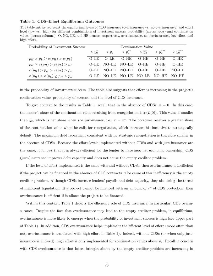
Table 1. CDS–Effort Equilibrium Outcomes

The table entries represent the equilibrium levels of CDS insurance (overinsurance vs. no-overinsurance) and effortlevel (low vs. high) for different combinations of investment success probability (across rows) and continuationvalues (across columns). O, NO, LE, and HE denote, respectively, overinsurance, no-overinsurance, low effort, andhigh effort.

Probability of Investment Success Continuation Value< y∗2 < y2 < y∗∗2 < y2 < y∗∗∗2 > y∗∗∗2

pH > pL ≥ c (pH) > c (pL) O–LE O–LE O–HE O–HE O–HE O–HE

pH ≥ c (pH) > c (pL) > pL O–LE NO–LE NO–LE O–HE O–HE O–HE

c (pH) > pH > c (pL) > pL O–LE NO–LE NO–LE O–HE O–HE NO–HE

c (pH) > c (pL) ≥ pH > pL O–LE NO–LE NO–LE NO–LE NO–HE NO–HE

in the probability of investment success. The table also suggests that effort is increasing in the project’s

continuation value, probability of success, and the level of CDS insurance.

To give context to the results in Table 1, recall that in the absence of CDSs, π = 0. In this case,

the lender’s share of the continuation value resulting from renegotiation is x (L(0)). This value is smaller

than y2, which is her share when she just-insures, i.e., π = π∗. The borrower receives a greater share

of the continuation value when he calls for renegotiation, which increases his incentive to strategically

default. The maximum debt repayment consistent with no strategic renegotiation is therefore smaller in

the absence of CDSs. Because the effort levels implemented without CDSs and with just-insurance are

the same, it follows that it is always efficient for the lender to have zero net economic ownership. CDS

(just-)insurance improves debt capacity and does not cause the empty creditor problem.

If the level of effort implemented is the same with and without CDSs, then overinsurance is inefficient

if the project can be financed in the absence of CDS contracts. The cause of this inefficiency is the empty

creditor problem. Although CDSs increase lenders’ payoffs and debt capacity, they also bring the threat

of inefficient liquidation. If a project cannot be financed with an amount of π∗ of CDS protection, then

overinsurance is efficient if it allows the project to be financed.

Within this context, Table 1 depicts the efficiency role of CDS insurance; in particular, CDS overin-

surance. Despite the fact that overinsurance may lead to the empty creditor problem, in equilibrium,

overinsurance is more likely to emerge when the probability of investment success is high (see upper part

of Table 1). In addition, CDS overinsurance helps implement the efficient level of effort (more often than

not, overinsurance is associated with high effort in Table 1). Indeed, without CDSs (or when only just-

insurance is allowed), high effort is only implemented for continuation values above y2. Recall, a concern

with CDS overinsurance is that losses brought about by the empty creditor problem are increasing in

26

continuation values. However, Table 1 shows that this effect is partially offset by the fact that effort is

also increasing in continuation values, which reduce the probability of inefficient liquidation.

Finally, note that the inefficiency of empty creditors is higher when the verification cost is lower (λ

is higher), which results in higher forgone renegotiation proceeds. However, from Proposition 10 one can

see that the cutoffs c (p∗), c (pH), and c (pL) are increasing in λ. This makes the equilibria depicted in

the lower part Table 1 more likely to obtain, implying less overinsurance.13

5.4.3 Constraints on CDS

According to the analysis of the last subsection, it is efficient for the lender to have zero net economic

ownership. This result questions the reform proposals supporting that lenders’ CDS positions should be

limited to positive net economic ownerships (e.g., Hu and Black (2008a,b)). Under that proposed re-

form, our model says that restructuring proceeds would be inefficiently reduced when zero net economic

ownership is optimal.

If the level of effort implemented under both zero and negative net economic ownerships are the same,

then overinsurance is inefficient if the project can be financed with just-insurance. If this is the case, pro-

posals to restrict net economic ownership to be non-negative would increase welfare (Bolton and Oehmke

(2011)). However, as pointed by our model, overinsurance minimizes agency problems by allowing the

implementation of high effort. When this happens, the gains brought about by overinsurance in terms

of higher probability of success can offset the losses caused by the empty creditor problem. Our analysis

suggests that banning CDS overinsurance may thus be unwarranted.

To characterize this latter point, we need to start by considering equilibria that result in overinsurance

and high effort in the absence of constraints on CDSs. These equilibria must then lead to low effort if we

ban CDS overinsurance. These scenarios are described in Table 1 by the outcomes with overinsurance and

continuation values above y2 and below y2. Total welfare with negative net economic ownership is given by

W− ≡ pH (y1 + y2) + (1− pH)βI, (9)

while welfare with zero net economic ownership is equal to

W0 ≡ pL (y1 + y2) + (1− pL) [1− δ (1− λ)] y2. (10)

13Although not depicted in Table 1, note that the expected inefficiency of CDS overinsurance is reduced by a betterverification technology (higher δ) and a higher recovery rate (β). The former implies higher verification costs and reducesthe proceeds from renegotiation, while the latter increases the proceeds from liquidation.

27

Since W− > W0 for pH sufficiently high, and W− < W0 for pH close to pL, there exists a cutoff

p∗H > pL such that for pH > p∗H it holds that W− > W0, and for pH < p∗H we have W− < W0. This result

says that a policy to cap net economic ownership to be nonnegative can reduce welfare. This and other

results derived in this section are summarized in Proposition 8.

Proposition 11. The following results hold regarding intervention and efficiency in CDS markets:

(1) For continuation values below y2 and above y2, overinsurance (restricting net economic ownership

to be nonnegative) is inefficient (efficient) if and only if the project can be financed without overin-

surance. The inefficiency (efficiency) of overinsurance is increasing (decreasing) in the projects’

continuation value and decreasing in its probability of success.

(2) For continuation values between y2 and y2, there exists a cutoff p∗H > pL such that overinsurance

(restricting net economic ownership to be nonnegative) is inefficient (efficient) if and only if pH <

p∗H .

(3) Just-insurance (restricting net economic ownership to be positive) is efficient (inefficient).

Proposition 11 shows that for continuation values that are either sufficiently high or small enough,

CDS markets can be inefficient if they lead to overinsurance and if projects can be financed without

CDSs. However, the inefficiency caused by the empty creditor problem is likely to be small in these cases.

High continuation values are associated with high effort and high probability of success, which reduces

the probability of default and liquidation.

For low continuation values, the inefficiency of empty creditors is reduced since forgone renegotiation

proceeds under liquidation are small. Our results suggest that constraining the lender’s net economic own-

ership to be nonnegative is unlikely to reduce the inefficiencies caused by the empty creditor problem. If

along with these results one also considers that CDSs increase lenders’ payoffs and debt capacity, then one

might conclude that not allowing for negative net economic ownership can be harmful. In fact, when the

probability of success is low, overinsurance only occurs for borrowers with low continuation values (ineffi-

ciency due to empty creditors is small). Accordingly, policies constraining CDSs are not only unlikely to

reduce the empty creditor problem, but also likely to reduce credit availability when firms need it the most.

For continuation values in the intermediary range, not allowing for CDS overinsurance can be inef-

ficient whether or not projects can be financed by overinsured creditors. Since overinsurance minimizes

the moral hazard problem and helps the implementation of high effort, it increases projects’ payoffs. This

28

is particularly true when agency problems are severe and the state of the economy is such that projects

are likely to succeed (“booms”). Our model thus casts doubt on the benefits of capping CDS insurance.

The results of this section characterize the role CDSs play in borrower–creditor relations and their

impact on the availability of credit. The analysis also discusses implications for optimal regulation. To

sum up, although CDS overinsurance may cause the empty creditor problem, our model shows that

overinsurance is more likely to be observed when expected inefficiencies associated with empty creditors

are lowest. In addition, we show that the efficient effort levels are generally induced along with overin-

surance, further reducing the probability of default and inefficient liquidation. The model implies that

these effects have an impact on credit availability, suggesting that they need to be more fully appreciated

by researchers in the field and policymakers.

6 Empirical Implications

We dedicate this section to the discussion of model implications. We do so presenting a non-exhaustive

list of testable empirical predictions, some of which are summarized in Table 1. We propose that examin-

ing these predictions would deepen our understanding of the CDS markets and their impact on corporate

financing and economic efficiency.

Implication #1: The incidence of negative net economic ownership is decreasing in firm risk.

This implication follows from the fact that safe firms have high probability of success, which implies

that lenders’ payoff lean more heavily on outcomes associated with investment success. As a result, the

extra debt repayment extracted when the project succeeds compensates for the forgone renegotiation

proceeds when the project fails.

Figure 2 provides evidence consistent with this implication. The figure plots the sum of the net par

amount of CDS protection bought by net buyers against reference entity risk, inversely represented by

the Altman Z-score. CDS notional amounts are in US dollars and are provided by the Deposit Trust

and Clearing Corporation (DTCC) for the thousand largest worldwide reference entities. The Altman

Z-score is calculated using data from Compustat and CRSP. The graph shows a significant and negative

correlation between CDS protection and firm risk.

Implication #2: Net economic ownership is countercyclical.

This implication is driven by firms for which the probability of investment success is closely tied to

economic conditions (“cyclical firms”). Booms result in higher probability of success, strengthening the

29

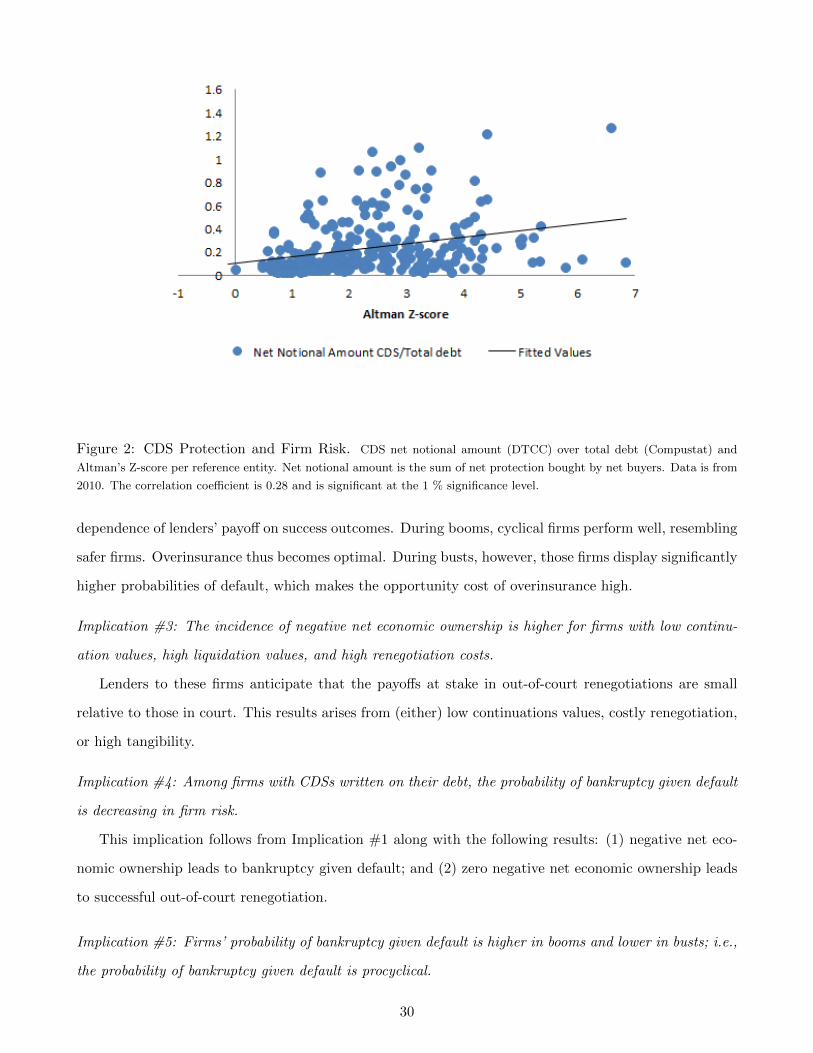
Figure 2: CDS Protection and Firm Risk. CDS net notional amount (DTCC) over total debt (Compustat) and

Altman’s Z-score per reference entity. Net notional amount is the sum of net protection bought by net buyers. Data is from

2010. The correlation coefficient is 0.28 and is significant at the 1 % significance level.

dependence of lenders’ payoff on success outcomes. During booms, cyclical firms perform well, resembling

safer firms. Overinsurance thus becomes optimal. During busts, however, those firms display significantly

higher probabilities of default, which makes the opportunity cost of overinsurance high.

Implication #3: The incidence of negative net economic ownership is higher for firms with low continu-

ation values, high liquidation values, and high renegotiation costs.

Lenders to these firms anticipate that the payoffs at stake in out-of-court renegotiations are small

relative to those in court. This results arises from (either) low continuations values, costly renegotiation,

or high tangibility.

Implication #4: Among firms with CDSs written on their debt, the probability of bankruptcy given default

is decreasing in firm risk.

This implication follows from Implication #1 along with the following results: (1) negative net eco-

nomic ownership leads to bankruptcy given default; and (2) zero negative net economic ownership leads

to successful out-of-court renegotiation.

Implication #5: Firms’ probability of bankruptcy given default is higher in booms and lower in busts; i.e.,

the probability of bankruptcy given default is procyclical.

30

This implication is a corollary of Implication #4 and suggests that CDS-led bankruptcy (out-of-court

restructuring) probabilities given distress are higher (lower) in booms. The opposite holds for busts.

Simply put, the empty creditor problem is procyclical.

Implication #6: Among firms with CDSs written on their debt, the incidence of agency costs is smaller

for firms with higher probability of success.

This implication follows from the fact that negative net economic ownership minimizes managers’

payoffs under default. The latter implies that managers have higher incentives to avoid default by im-

plementing high effort, hence increasing the probability of success.

While our model’s predictions are new and have not been directly taken to the data, some reported

empirical regularities are consistent with our theory. We argue, for example, that CDSs are more ben-

eficial for firms that are safer and have higher continuation values. This result is interesting and stands

in contrast to common intuition that riskier firms would benefit the most from the existence of CDS

markets. Consistent with our theory, however, recent studies by Ashcraft and Santos (2009) and Hirtle

(2009) find that safer and larger firms have benefited the most from CDS contracts (for example, by

paying lower spreads on their bank loans). Song and Uzmanoglu (2010) explore the Financial Crisis and

find evidence that firms associated with safer banks (typically safer firms) observed smaller CDS spreads

in the 2008–9 period.

Another unintuitive prediction of our model is the procyclicality of the empty creditor problem. This

implies that the conditional probability of CDS-led bankruptcy given that a firm is in distress is higher

in booms. Interestingly, starting with the prior that CDSs aggravate the empty credit problems in busts

— the opposite of our model’s prediction — Bedendo et al. (2010) fail to find evidence that the CDS

contracting leads to a higher incidence of bankruptcies (relative to out-of-court restructurings) during

the Financial Crisis (see also Mengle (2009) and Aspeli and Iden (2010)).

A number of other predictions listed above can be directly taken to the data. Empirical research on

CDS is still in its infancy and this strikes us as setting in which models describing rich sets of creditor–

borrower relations are particularly useful in guiding empirical work.

7 Concluding Remarks

Financial innovation is the hallmark of capital markets in developed economies. At the same time, fi-

nancial innovations have also preceded virtually all major economic crises in history (see Kindleberger

31

(2000)). The 2008–9 crisis has brought renewed interest in innovation and regulation of financial markets.

A great deal of attention, in particular, has been given to CDS contracts as these derivatives seemed to

play a role in the demise of numerous banks and industrial firms during the crisis. Examples range from

Lehman Brothers to GM and Six Flags. We argue that while we might have observed a high degree of

association between bankruptcies and CDS contracts during the crisis, it is hard to conclude that CDSs

led to excessive, inefficient liquidation in that period. To draw that inference, one needs a benchmark

model describing the connections between CDS contracting and the economy.

We develop a model of optimal CDS contracting when investment is subject to moral hazard and

wealth verification is imperfect. To our knowledge, this model is the first to show how lenders choose

between debt payments and restructuring proceeds — accounting for the state of the economy — when

selecting the optimal amount of CDS protection. Counter to previous arguments in the literature, we

show that CDS overinsurance is more likely to occur in booms, when it boosts firm debt capacity and

increases the number of projects with positive NPV that receive funding. CDS contracts alleviate credit

rationing during recessions, but in those times CDS overinsurance may prompt the liquidation of firms

with less promising prospects (firms that would likely be rationed in the absence of CDS). Our model

demonstrates that the empty creditor problem is procyclical. Moreover, it implies that the casual ob-

servation that CDS contracts are associated with bankruptcies in the crisis does not imply that those

contracts harm financial efficiency.

A number of recent proposals aim at constraining the amount and ownership of CDS contracts on a

firm’s debt. Most notably, they suggest that the degree CDS-based insurance should be lower than —

or, at a maximum, equal to — the amount of economic exposure of lenders. Our paper cautions about

the potential effects of these proposals on the availability of credit and on financing efficiency. Complex

contracts such as CDSs are inexorably linked to the forms of financing arrangements we will be seeing in

future years, as financial markets become more sophisticated and integrated. One has to be careful about

imposing constraints on the markets for these contracts at an early stage of their development. At the

same time, one needs to better understand how these contracts work and the types of inefficiencies they

address. In this way, one might be able to more fully benefit from what these contracts have to offer.

32

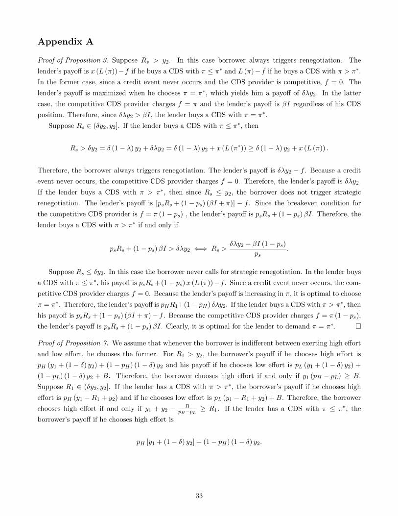
Appendix A

Proof of Proposition 3. Suppose Rs > y2. In this case borrower always triggers renegotiation. The

lender’s payoff is x (L (π))−f if he buys a CDS with π ≤ π∗ and L (π)−f if he buys a CDS with π > π∗.

In the former case, since a credit event never occurs and the CDS provider is competitive, f = 0. The

lender’s payoff is maximized when he chooses π = π∗, which yields him a payoff of δλy2. In the latter

case, the competitive CDS provider charges f = π and the lender’s payoff is βI regardless of his CDS

position. Therefore, since δλy2 > βI, the lender buys a CDS with π = π∗.

Suppose Rs ∈ (δy2, y2]. If the lender buys a CDS with π ≤ π∗, then

Rs > δy2 = δ (1− λ) y2 + δλy2 = δ (1− λ) y2 + x (L (π∗)) ≥ δ (1− λ) y2 + x (L (π)) .

Therefore, the borrower always triggers renegotiation. The lender’s payoff is δλy2 − f . Because a credit

event never occurs, the competitive CDS provider charges f = 0. Therefore, the lender’s payoff is δλy2.

If the lender buys a CDS with π > π∗, then since Rs ≤ y2, the borrower does not trigger strategic

renegotiation. The lender’s payoff is [psRs + (1− ps) (βI + π)] − f . Since the breakeven condition for

the competitive CDS provider is f = π (1− ps) , the lender’s payoff is psRs + (1− ps)βI. Therefore, the

lender buys a CDS with π > π∗ if and only if

psRs + (1− ps)βI > δλy2 ⇐⇒ Rs >δλy2 − βI (1− ps)

ps.

Suppose Rs ≤ δy2. In this case the borrower never calls for strategic renegotiation. In the lender buys

a CDS with π ≤ π∗, his payoff is psRs+(1− ps)x (L (π))−f . Since a credit event never occurs, the com-

petitive CDS provider charges f = 0. Because the lender’s payoff is increasing in π, it is optimal to choose

π = π∗. Therefore, the lender’s payoff is pHR1+(1− pH) δλy2. If the lender buys a CDS with π > π∗, then

his payoff is psRs + (1− ps) (βI + π)− f . Because the competitive CDS provider charges f = π (1− ps),the lender’s payoff is psRs + (1− ps)βI. Clearly, it is optimal for the lender to demand π = π∗.

Proof of Proposition 7. We assume that whenever the borrower is indifferent between exerting high effort

and low effort, he chooses the former. For R1 > y2, the borrower’s payoff if he chooses high effort is

pH (y1 + (1− δ) y2) + (1− pH) (1− δ) y2 and his payoff if he chooses low effort is pL (y1 + (1− δ) y2) +

(1− pL) (1− δ) y2 + B. Therefore, the borrower chooses high effort if and only if y1 (pH − pL) ≥ B.

Suppose R1 ∈ (δy2, y2]. If the lender has a CDS with π > π∗, the borrower’s payoff if he chooses high

effort is pH (y1 −R1 + y2) and if he chooses low effort is pL (y1 −R1 + y2) +B. Therefore, the borrower

chooses high effort if and only if y1 + y2 − BpH−pL ≥ R1. If the lender has a CDS with π ≤ π∗, the

borrower’s payoff if he chooses high effort is

pH [y1 + (1− δ) y2] + (1− pH) (1− δ) y2.

33

The borrower’s payoff if he chooses low effort is

pL [y1 + (1− δ) y2] + (1− pL) (1− δ) y2 +B.

Therefore, the borrower chooses high effort if and only if y1 (pH − pL) ≥ B. Suppose R1 ≤ δy2. The

borrower’s payoff is he chooses high effort is

pH [y1 −R1 + y2] + (1− pH) (1− δ) y2.

The borrower’s payoff is he chooses low effort is

pL [y1 −R1 + y2] + (1− pL) (1− δ) y2 +B.

Therefore, the borrower chooses high effort if and only if

y1 + δy2 −B

pH − pL≥ R1,

which concludes the proof.

Proof of Proposition 8. One must note that (1) and (3) follow directly from Propositions 4 and 5. For

(2), let R1 ∈ (R (0) , y2]. One must note that R1 > R (0) ≥ R (µ), which implies that the lender buys

a CDS with π > π∗. If R1 > R1, then the borrower chooses eL, which implies µ = 0. Therefore

(π > π∗, e = eL, µ = 0) is the unique equilibrium of the CDS–Effort game, which establishes (a). If

R1 ≤ R1, then the borrower chooses eH and we have µ = 1. As a result, R1 > R (0) ≥ R (1) and

(π > π∗, e = eH , µ = 1) is the unique equilibrium of the CDS–Effort game, which establishes (b).

Let R1 ∈ (δy2, R (0)]. Suppose R1 > R1. If µ is such that R1 > R (µ), the lender chooses π > π∗.

The borrower chooses eL, which implies µ = 0. But then we have a contradiction since R1 ≤ R (0) and

choosing π = π∗ is optimal for the lender. If µ is such that R1 ≤ R (µ), the lender chooses π = π∗. The

borrower chooses eL, which implies µ = 0. Therefore, R1 ≤ R (µ) ≤ R (0) and (π = π∗, e = eL, µ = 0) is

the unique equilibrium of the CDS–Effort game.

Suppose R1 ≤ R1. If µ is such that R1 > R (µ), the lender chooses π > π∗. The borrower chooses eH ,

which implies µ = 1. Therefore, R1 > R (µ) ≥ R (1) and (π > π∗, e = eH , µ = 1) is an equilibrium. If µ

is such that R1 ≤ R (µ), the lender chooses π = π∗. As a consequence, the borrower chooses eL, which

implies µ = 0. Therefore, R1 ≤ R (µ) ≤ R (0) and (π = π∗, e = eL, µ = 0) is an equilibrium.

Proof of Proposition 9. Suppose R1 is such that R1 ≤ δy2. Without loss of generality, let R1 ∈ [0, δy2]. If

the lender chooses R1 = R1, then the borrower chooses eH , the lender buys a CDS with π = π∗, and con-

sistency of beliefs implies µ = 1. We know that the borrower does not call for strategic renegotiation. The

lender’s expected payoff is pHR1 + (1− pH) δλy2. If the lender chooses δy2 = R1, the borrower chooses

eL, the lender buys a CDS with π = π∗, and consistency of beliefs implies µ = 0. We know that the

34

borrower does not call for strategic renegotiation. The lender’s expected payoff is pLR1 + (1− pL) δλy2.

The lender chooses R1 = R1 if and only if y2 ≥ y2 ≡ − pHδ(pH−pL)(1−λ)∆.

Suppose he chooses R1 ∈ (δy2, y2]. If the lender chooses R1 = R1, then the borrower chooses eH , the

lender buys a CDS with π > π∗, and consistency of beliefs implies µ = 1. The borrower does not trigger

strategic renegotiation. The lender’s expected payoff is pHR1+(1− pH)βI. If the lender chooses R1 = y2,

then the borrower chooses eL, the lender buys a CDS with π > π∗, and consistency of beliefs implies µ = 0.

The borrower does not call for strategic renegotiation. The lender expected payoff is pLy2 + (1− pL)βI.

The lender chooses R1 = R1 if and only if pHR1 + (1− pH)βI ≥ pLy2 + (1− pL)βI ⇐⇒ y2 ≥ y2 ≡− pHpH−pL ∆ + βI. If R1 > y2 then the borrower chooses eL, the lender buys a CDS with π = π∗, and

consistency of beliefs implies µ = 0. The borrower triggers strategic renegotiation. The lender’s payoff is

δλy2.

Proof of Proposition 10. We have max{

Π (y2) ,Π(R1

)}= Π (y2) and max

{Π (δy2) ,Π

(R1

)}= Π (δy2)

for y2 < y2. Since Π (y2) > Π (δy2) for y2 small, there exists y∗2 such that Π (y∗2) = Π (δy∗2) if and only

if the slope of Π (δy2) is higher than that of Π (y2). This is true if and only if c (pL) > pL. In this

case, direct calculations show that y∗2 < y2 if and only if the liquidation value is sufficiently small, i.e.,

βI < −pH∆[c(pL)−pL](pH−pL)[1−c(pL)] . We also have that max

{Π (y2) ,Π

(R1

)}= Π

(R1

)and max

{Π (δy2) ,Π

(R1

)}=

Π (δy2) for y2 ≤ y2 < y2. Since Π (δy2) > Π(R1

)for y2 small, there exists y∗∗2 such that Π (δy∗∗2 ) = Π

(R1

)if and only if the slope of Π

(R1

)is higher than that of Π (δy2). This is true if and only if pH > c (pL).

Finally, we have that max{

Π (y2) ,Π(R1

)}= Π

(R1

)and max

{Π (δy2) ,Π

(R1

)}= Π

(R1

)for y2 ≥ y2.

Since Π(R1

)> Π

(R1

)for y2 small, there exists y∗∗∗2 such that Π

(R1

)= Π

(R1

)if and only if the slope

of Π(R1

)is higher than that of Π

(R1

). This is true if and only if c (pH) > pH .

Case 1 (pH > pL ≥ c (pH) > c (pL)): In this case, the lender chooses R1 = y2 for y2 < y2 and

R1 = R1 for y2 ≥ y2. It must follow that R1 = R1 for y2 ≤ y2 < y2. To see this, suppose otherwise, i.e.,

y∗∗2 is such that either y∗∗2 ≥ y2 or y2 < y∗∗2 < y2. If the latter holds then, because Π (y2) > Π (δy2) for

all y2, we have Π (y2) > Π (δy2) > Π(R1

)for y2 < y2 < y∗∗2 . But this contradicts the definition of y2.

If the former holds then, because Π(R1

)> Π

(R1

)for all y2, we have Π (δy2) ≥ Π

(R1

)> Π

(R1

)for

y2 ≤ y2 ≤ y∗∗2 . This contradicts the definition of y2.

Case 2 (pH ≥ c (pH) > pL ≥ c (pL)): The analysis is the same as in case Case 1.

Case 3 (pH ≥ c (pH) > c (pL) > pL): In this case, the lender chooses R1 = R1 for y2 ≥ y2. There are

two cases to consider: (1) y∗2 ≥ y2 and (2) y∗2 < y2. If (1) holds, then we are back to Cases 1 and 2 as R1 =

y2 for y2 < y2 and R1 = R1 for y2 ≤ y2 < y2. The former follows by assumption since Π (y2) > Π (δy2) for

all y2 such that y2 < y2, which establishes. For the latter, suppose otherwise, i.e., y∗∗2 > y2. First, let y2 <

y∗∗2 < y2. If y∗2 is such that y2 ≤ y∗2 < y∗∗2 , then we have Π (y2) ≥ Π (δy2) > Π(R1

)for y2 ≤ y2 ≤ y∗2, which

contradicts the definition of y2. If y∗2 ≥ y∗∗2 , then we have Π (y2) > Π (δy2) > Π(R1

)for y2 < y2 < y∗∗2 ,

which also contradicts the definition of y2. Second, let y∗∗2 ≥ y2. In this case, because Π (y2) > Π (δy2)

for all y2, we have Π (δy2) ≥ Π(R1

)> Π

(R1

)for y2 ≤ y2 ≤ y∗∗2 , which contradicts the definition of y2.

If (2) holds, then R1 = y2 for y2 < y∗2 and R1 = δy2 for y∗2 ≤ y2 < y2. This implies y2 < y∗∗2 < y2

such that R1 = δy2 for y2 ≤ y2 < y∗∗2 and R1 = R1 for y∗∗2 ≤ y2 < y2. To see this, suppose otherwise.

i.e., either y∗∗2 ≥ y2 or y∗∗2 < y2. If y∗∗2 ≥ y2 then, since Π(R1

)> Π

(R1

)for all y2, we have that

Π (δy2) ≥ Π(R1

)> Π

(R1

)for y2 ≤ y2 ≤ y∗∗2 , which contradicts the definition of y2. If y∗∗2 < y2, then we

35

have that Π(R1

)> Π (δy2) > Π (y2) for y∗∗2 < y2 < y2, which contradicts the definition of y2.

Case 4 (c (pH) > c (pL) ≥ pH > pL): In this case, the lender chooses R1 = δy2 for y2 ≤ y2 < y2.

This implies that y∗∗∗2 ≤ y2. To see this, suppose otherwise, i.e., y∗∗∗2 > y2. Since Π (δy2) > Π(R1

)for all y2, we have that Π (δy2) > Π

(R1

)> Π

(R1

)for y2 ≤ y2 < y∗∗∗2 . But this contradicts the def-

inition of y2. Therefore, it follows that y∗∗∗2 ≤ y2, which implies that R1 = R1 for y2 ≥ y2. Finally,

it must be that y∗2 < y2. To see this, suppose otherwise, i.e., y∗2 ≥ y2. If y∗2 < y2, then we have that

Π (y2) ≥ Π (δy2) > Π(R1

)for y2 ≤ y2 ≤ y∗2, which contradicts the definition of y2. If y∗2 ≥ y2, then

Π (y2) ≥ Π (δy2) > Π(R1

)for y2 ≤ y2 < y2, which also contradicts the definition of y2.

Case 5 (c (pH) > pH > pL ≥ c (pL)): This case is impossible. To see this note that, by the definition

of c (p), p ≥ c (p) if and only if p ≥ δλ + δ (1− λ) p, which is true if and only if p ≥ δλ1−δ(1−λ) . But this

implies that pL ≥ δλ1−δ(1−λ) > pH , which contradicts the assumption that pH > pL.

Case 6 (c (pH) > pH > c (pL) > pL): There are two cases to consider: (1) y∗2 ≥ y2 and (2) y∗2 < y2.

If (1) holds, then from Case 3 we know that R1 = y2 for y2 < y2 and R1 = R1 for y2 ≤ y2 < y2. It also

follows that y∗∗∗2 ≥ y2. To see this, suppose otherwise, i.e., y∗∗∗2 < y2. If y∗∗∗2 ≥ y2, then we have that

Π(R1

)≥ Π

(R1

)> Π (δy2) for y∗∗∗2 ≤ y2 < y2, which contradicts the definition of y2. If y∗∗∗2 < y2, then

Π(R1

)≥ Π

(R1

)> Π (δy2) for y2 ≤ y2 < y2, which also contradicts the definition of y2.

If Case 2 holds, then from Case 3 we know that R1 = y2 for y2 < y∗2 and R1 = δy2 for y∗2 ≤ y2 < y2.

If y∗∗2 ≥ y2, then the lender chooses R1 = δy2 for y2 ≤ y2 < y2. This implies that we are back to Case

4, from which it follows that y∗∗∗2 ≤ y2 and the lender chooses R1 = R1 for y2 ≥ y2. If y∗∗2 < y2, then

it must be that y2 < y∗∗2 < y2. To see this, suppose otherwise, i.e., y∗∗2 ≤ y2. For y∗∗2 > y∗2, it follows

that Π(R1

)≥ Π (δy2) > Π (y2) for y∗∗2 ≤ y2 ≤ y2, which contradicts the definition of y2. For y∗∗2 ≤ y∗2,

it follows that Π(R1

)> Π (δy2) > Π (y2) for y∗2 < y2 < y2, which also contradicts the definition of y2.

Therefore, the lender chooses R1 = δy2 for y2 ≤ y2 < y∗∗2 and R1 = R1 for y∗∗2 ≤ y2 < y2. Finally, it

follows that y∗∗∗2 ≥ y2. To see this suppose otherwise, i.e., y∗∗∗2 < y2. If y∗∗∗2 ≥ y∗∗2 , then we have that

Π(R1

)> Π

(R1

)> Π (δy2) for y∗∗∗2 < y2 < y2, which contradicts the definition of y2. If y∗∗∗2 < y∗∗2 , then

we have that Π(R1

)> Π

(R1

)≥ Π (δy2) for y∗∗2 ≤ y2 < y2, which also contradicts the definition of y2.

36

References

[1] Arping, S., 2004, “Credit Protection and Lending Relationships,” Working Paper, University ofAmsterdam.

[2] Ashcraft, A., and J. Santos, 2009, “Has the CDS Market Lowered the Cost of Corporate Debt?”Journal of Monetary Economics 56, 514–523.

[3] Aspeli, N., and K. Iden, 2010, “The Empty Creditor Hypothesis: An Empirical Study of the Effectsof Credit Insurance on the Choice between Bankruptcy and Private Restructuring,” Master Thesis,Norwegian School of Economics and Business Administration.

[4] Bedendo, M., L. Cathcart, and L. El-Jahel, 2010, “In- and Out-of-Court Debt Restructuring in thePresence of Credit Default Swaps,” Working Paper, Imperial College.

[5] Bolton, P., and M. Oehmke, 2011, “Credit Default Swaps and The Empty Creditor Problem,” Reviewof Financial Studies 24, 2617–2655.

[6] Bolton, P., and D. Scharfstein, 1990, “A Theory of Predation Based on Agency Problems in FinancialContracting,” American Economic Review 80, 93–106.

[7] Calomiris, C., and C. Kahn (1991), “The Role of Demandable Debt in Structuring Optimal BankingArrangements,” American Economic Review 81, 497–513.

[8] Diamond, D., and R. Rajan, 2001, “Liquidity Risk, Liquidity Creation, and Financial Fragility: ATheory of Banking,” Journal of Political Economy 109, 287–327.

[9] Duffee, G. R., and C. Zhou, 2001, “Credit Derivatives in Banking: Useful Tools for Managing Risk?”Journal of Monetary Economics 48, 25–54.

[10] Hart, O., and J. Moore, 1994, “A Theory of Debt Based on the Inalienability of Human Capital,”Quarterly Journal of Economics 109, 841–879.

[11] Hart, O., and J. Moore, 1998, “Default and Renegotiation: A Dynamic Model of Debt,” QuarterlyJournal of Economics 113, 1–41.

[12] Hu, H., and B. Black, 2007, “Hedge Funds, Insiders, and the Decoupling of Economic and VotingOwnership: Empty Voting and Hidden (Morphable) Ownership,” Journal of Corporate Finance 13,343–367.

[13] Hu, H., and B. Black, 2008a, “Debt, Equity, and Hybrid Decoupling: Governance and Systemic RiskImplications,” European Financial Management 14, 663–709.

[14] Hu, H., and B. Black, 2008b, “Equity and Debt Decoupling and Empty Voting II: Importance andExtensions,” University of Pennsylvania Law Review 156, 625–739.

[15] Hirtle, B., 2009, “Credit Derivatives and Bank Credit Supply,” Journal of Financial Intermediation18, 125–150.

[16] Kindleberger, C., 2000, Manias, Panics, and Crashes: A History of Financial Crises, John Wiley &Sons, Inc., New York.

[17] Krasa, S., and A. Villamil, 2000, “Optimal Contracts When Enforcement is a Decision Variable,”Econometrica 68, 119–134.

[18] Mengle, D., 2009, “The Empty Creditor Hypothesis,” International Swaps and Derivatives Associa-tion (ISDA) Research Notes No. 3.

[19] Morrison, A. C., 2005, “Credit Derivatives, Disintermediation, and Investment Decisions,” Journalof Business 78, 621–647.

37

[20] Parlour, C. A., and G. Plantin, 2008, “Loan Sales and Relationship Banking,” Journal of Finance63, 1291–1314.

[21] Parlour, C., and A. Winton, 2008, “Laying off Credit Risk: Loan Sales versus Credit Default Swaps,”Working Paper, University of California at Berkeley.

[22] Saretto, A., and H. Tookes, 2013, “Corporate Leverage, Debt Maturity and Credit Default Swaps:The Role of Credit Supply,” Review of Financial Studies 26, 1190–1247.

[23] Roberts, M., and A. Sufi, 2009, “Renegotiation of Financial Contracts: Evidence from Private CreditAgreements, ” Journal of Financial Economics 93, 159–184. University.

[24] Song, W., and C. Uzmanoglu , 2010, “Systemic Risk Channel: Banking Relationship Spillover in theCredit Default Swaps and Stock Markets,” Working Paper, Louisiana State University.

38