Credit-Based Flow Control for ATM Networks:Credit Update Protocol, Adaptive Credit Allocation, and Statistical Multiplexing

H. T. Kungl, Trevor Blackwelll) 2 and Alan Chapman2

lDivision of Applied Sciences, Harvard University, 29 Oxford Street, Cambridge, MA 02138, USA

2Be11-Northem Research, P.O.Box 3511, Station C, Ottawa, Ontario KIY 4H7, Canada

Abstract

This paper presents three new results concerning credit-based

jlow control for ATIU network: (1) a simple and robust credit

up~te pro@col (CUP) suited for relatively inexpensive hardwareiso+are implementation; (2) automatic adaptation of credit bufjer

allocation for virtual circuits (VCS) sharing the same bujfer pool;

(3) use of credit- based$ow control to improve the effectiveness of

statistical multipltning in mim”mizing switch memory. These results

hme been substantiated by anulysis, simulation and implementa-

tion.

1. Introduction

Flow control is essential for asynchronous transfer mode

(ATM) networks [1] in providing “best-effort” services, or ABR

(Available Bit Rate) services in the ATM Forum terminology. With

proper flow control, computer users would be able to use an ATM

network in the same way as they have been using conventional

LANs, namely, they can use the network at any time without first

negotiating a “traffic contract” with the network. Any one user

would be able to acquire as much network resources as are avail-

able at any given momen~ and all users compete equally for the

available bandwidth.

An efficient way of implementing flow-controlled ATM

networks is through the use of credit-based, per VC, link-by-link

flow control [11]. This paper gives several new results related to

the credh-baaed flow control. All the VCS are assumed to be under

“best-effort” or ABR services, unless stated otherwise.

The organization of the paper is as follows: Fks4 motivations

for per VC, link-by-link flow con~ol are given. This is followed by

an overview of the credit-based flow control approach and a

summary of its advantages. Then three main results of this results

are preserttetb

This research was supported in part by BNR, and in part by the

Advanced Research Projects Agency (DOD) monitored by ARPA/

CMO under Contract MDA972-90-C-O035 and by AFMC under

Conhact F19628-92-C-0116.

Permission to co y without fee all or part of this material is1!granted provided t at the copies are not made or distributed for

direct commercial advanta$e, the ACM copyright notice and thetitle of the publication and Its date appear{ and notice is giventhat copying is by permission of the Association of ComputingMachinery. To copy otherwise, or to republish, requires a feeand/or specific permission.SIGCOMM 94 -8/94 London England UK@ 1994 ACM 0-89791 -682-4/94/0008..$3.50

.

.

.

In Section 5, we describe a credit update protocol (CUP),

which allows relatively simple hardware/softwme implemen-

tation and is robust against transient errors.

In Section 6, we describe an adaptive credit allocation scheme

where a number of VCS can dynamically share the same buffer

pool while still guaranteeing no data loss due to congestion

and ensuring high link utilization. The credit buffer allocated

to an individual VC will adjust automatically according to the

actuat bandwidth usage of the VC. There are two advantages

of this adaptation capability. First, since the credit buffer size

can be derived automatically, there is no need for the user or

the system to specify it. This significantly eases the use and

implementation of “best-effort” or ABR services. Second,

since inactive VCS can automatically yield their unused buffer

space to other active ones, the total buffer size required by the

flow-controlled VCS at the node can be minimized. Irtpractice,

the total buffer for all the VCS need not be Lwger than a small

multiple of the product of the link bandwidth and round-trip

link propagation delay. We present simulation results demon-

strating the effectiveness of this adaptive credit scheme.

In Section 7, we note that credh-based flow control can help

statistical multiplexing in minimizing switch memory. This

result is especially useful for WAN switches which may have

to depend on statistical multiplexing to reduce the odterwise

large memory required to cover large propagation delays.

Credh-baaed flow control can help because it will automati-

cally lirrth burst sizes to be no more than the allocated credit

size, thereby improving the effectiveness of statistical multi-

plexing. We present simulation results demonstrating signifi-

cant memory reduction while achieving zero or low rate of cell

loss. The approach is particularly attractive for tiaffic with

large bursts for which statistical multiplexing without flow

control would perform poorly.

These three results are complementary. CUP provides a base-

line, efficient and robust protocol for implementing credit-based

flow wntrol. Adaptive credit allocation allows efficient sharing of

a given buffer pool between multiple VCS, and eases the use of

credit-based flow control. Improved statistical multiplexing due to

credit-based flow control will allow a switch memory of the same

size to serve an expanded number of VCS and to handle links of

increased propagation delays.

Aversion of the proposed credh-based flow control scheme has

been implemented on an experimental Am switch with 622-

101

Mbps ports, currently under joint development by BNR and

Harvard. This switch will be operational in fall 1994.

2. Why Per VC Link-by-Link Flow Control?

The Flow-Controlled Virtual Connections (FCVC) approach

[11], using per VC, link-by-link flow control, is different from

other propmtls on congestion control (see, e.g., [2, 8, 15]). Our

interest in FCVC is primarily due to its effectiveness in maxi-

mizing network utilization, controlling wngestion, and imple-

menting “best-effort” or ABR services.

2.1. Maximizing Network Utilization

FCVC provides effective means of using fill-in traffic to maxi-

mize network utilization, as depicted in Figure 1. Using FCVC,

best-effort traffic can effectively M in bandwidth slack left by

scheduled traffic with guaranteed bandwidth and latency such as

video and audio. In the fill-in process, various scheduling policies

can be employed. For example, high-priority best-effort traffic can

be used in the fill in before the low-priority one.

Fill in “Best-Effort” Traffic

Time “Figure 1: Fill in bandwidth slacks with “best-effort” trafiic

For effective traffic M in, fast congestion feedback for indi-

vidual VCS is needed. Measurements have shown that data [6, 13]

and video [7] traffic often exhibit large bandwidth variations even

over time intervals SSsmall 55 10 milliseconds. Whh the emerg-

ence of very high-bandwidth traffic sources such as high-speed

host computers with 800-Mbps HIPPI network [3] interfaces,

networks will experience further increases in load fluctuations

[10]. To utilize slack bandwidth in the presence of highly bursty

traftic, fast congestion feedback is necessary.

To illustrate the need of fast feedback or flow control for effec-

tive fill in, wnsider a simple case of maxtilzing the utilization of

a iii. As depicted in Figure 2, there are multiple VCS from the

sender to the receiver sharing the link. The VC scheduler at the

sender selects (when possible), for each cell cycle, a VC from

which a cell will Ix transmitted over the link. It is intuitively clear

how the scheduler should work that is, after satisfying VCS of

guaranteed performance, the scheduler will select other VCS (“fill-

irt” VCS), with high priority ones first, to fill in the available band-

width of the link.

However, two additional wndltions (both requiring fast flow

control) must be satisfied in order to achieve effective fill in:

● FirsL data to be used for fill in must be “drawn” to the sender

in time. That is, these fill-in VCS should try to hold in their

buffers at the sender a number of cells that are ready to be

forwarded. There should be sufficiently many of these cells so

that they can fill in slack bandwidth at a high rate as soon as

the bandwidth bewmes available. Note that how long these

cells will stay at the sender depends on the load of other VCS.

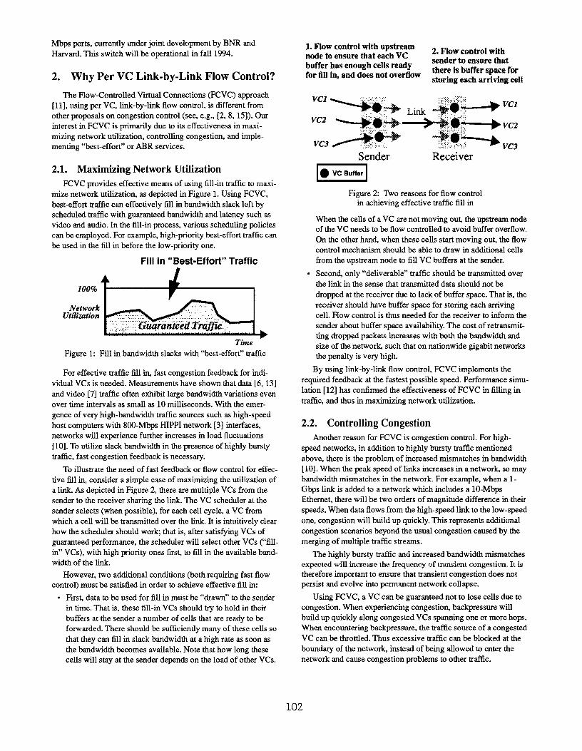
L Flow control with upstreamnode to ettsure that each VC

2. Flow COilti’01 with

tmffer has enough cells readysender to ensttre thatthere is buffer space for

for fill in, md does tmt overflow tirkg ~ch ~tivhg cell

‘“1 ~~h Link $@~ ‘C2

‘=2 +w-’&+:@;&+vc2%&,+vc,

““3 &;#”-@ .:,,,,,:,:,,,:

Sender Receiver

.

kx2!ElFigure 2: Two reasons for flow control

in achieving effective trat%c fill in

When the cells of a VC are not moving ou~ the upslrearn node

of the VC needs to be flow controlled to avoid buffer overflow.

On the other hand, when these cells start moving out, the flow

control mechanism should be able to draw in additional cells

from the upstream node to fill VC buffers at the sender.

Second only “deliverable” traffic should be tmnsmitted over

the link in the sense that transmitted data should not be

dropped at the receiver due to lack of buffer space. That is, tbe

receiver should have buffer space for storing each arriving

cell. Flow control is thus needed for the receiver to inform the

sender about buffer space availability. The cost of retransmit-

ting dropped packets increases with both the bandwidth and

size of the networh such that on nationwide gigabit networks

the penalty is very high.

By using link-by-link flow control, FCVC implements the

required feedback at the fastest possible speed. Performance simu-

lation [12] has wnfirrned the effectiveness of FCVC in filling in

traflic, and thus in maximizing network utilization.

2.2. Controlling Congestion

Another reason for FCVC is wngestion wntrol. For high-

speed networks, in addition to highly bursty traffic mentioned

above, there is the problem of increased mismatches in bandwidth

[10]. When the peak speed of links increases in a network so may

bandwidth mismatches in the network. For example, when a 1-

Gbps link is added to a network which includes a 10-Mbps

Ethernet, there will be two orders of magnitude difference in their

speeds. When data flows from the high-speed link to the low-speed

one, congestion will build up quickly. This represents additional

congestion scenarios beyond the usual wngestion caused by the

merging of multiple traffic s~esrns.

The highly bursty tnffic and increased bandwidth mismatches

expected will increase the frequency of mmsient congestion. It is

therefore important to ensure that transient congestion does not

persist and evolve into permanent network collapse.

Using FCVC, a VC can be guaranteed not to lose cells due to

congestion. When experiencing congestion, backpressure will

build up quickly along wngested VCS spanning one or more hops.

When encountering backpressure, the &affIc source of a congested

VC can be throttled. Thus excessive traffic can be blocked at the

boundary of the network, instead of being allowed to enter the

network and cause congestion problems to other traffic.

102

By using “per VC” flow control, FCVC allows multiple VCS

over the same physical link to operate at different speeds,

depending on their individual congestion status. In particular,

congested VCS cannot block other VCS which are not congested.

The throttling feahtre on individual VCS, enabled by FCVC, is

especially useful for implementing high-performance, reliable

multicast VCS. At any mukicasting point involving more than a

few ports, the delay before a cell is forwarded out all the ports cart

fluctuate greatly. It is therefore essential for reliable multicast VCS

to throttle in order to accommodate the inherent high wwiations in

their transmission speeds. Thus, the credit value can be based on

the slowest port (the one with the largest queue) to ensure that no

buffer will be overrun. Of course, in practice a “relatively” reliable

multicast which allows some sort of time-out on blocked multi-

casting ports will be implemented so that an blocked port will not

hold up the whole multicast VC for an unbounded amount of time.

2.3. Implementing “Best-Effort” or ABR Services

Flow control will enable services for hosts with high-speed

network access links operating, for example, at 155 Mbps. For

instance, these hosts can be offered anew kmd of data cotnmunica-

tions service, which maybe called a “gr=dy” service, where the

network will accept as much traffic as it has available bandwidth at

any instant from VCS under this service. FCVC can throttle these

VCS on a per VC basis when the network load becomes too high,

and also speed them up when the load clears. This is exactly the

traditional “best-effort” service typical for hosts in LAN environ-

ments. There will be no requirements for predefmed service

contract parameters, which are difficult to set.

3. Credit-Based Flow Control

Flow control based on credits is ,an efficient way of imple-

menting per VC link-by-link flow control. A credit-based flow

control method generally works over each flow-controlled VC link

as follows (see Figure 3). Before forwarding any data cell over the

~ the sender needs to receive credits for the VC via credit cells

sent by the receiver. At various times, the receiver sends credit

cells to the sender indicating availability of buffer space for

receiving data cells of the VC. After having received credits, the

sender is eligible to forward some number of data cells of the VC

to the receiver according to the received credit information. Each

time the sender forwards a data cell of a VC, it decrements its

current credit Mance for the VC by one.

~-o

H- ...? ‘“’3,,*=- “*? ‘:v+k’ch 2

/

,,, ,,,,,’,

A%EID.@!!l!l~~ :..“cl /%- ‘* ., ,;,:,,

.::; Switch 1,,,.,:?l,,, ,,,.,,,,,,.,,,-..,,.,..,,, ,,,,,:,,,,,, ,,.,,,,,,,.,,,,,,,,, ..::.

VC2:*W,,,,,,,,,,,,,,,,.,,.,,,,,,,,,.,.

~h

,,,,.,,,,,,,,,,,,,,,,,,,,,,..*,,, .,.,,., ,,~;t ~“ lmltlW’?Jy&.’.,,,,, :

h..’ :~”Hast 2‘* *:”,,,. .,,

F@re 3: Credit-based flow control

applied to each link of a VC

4. The iV23 Scheme: A Credit-Based FlowControl Scheme

The “N23 Scheme” is a specific scheme for implementing

credh-bssed flow control over a link. (The method is called N23

for reasons to be explained later.) This section provides an easy-to-

understand, theoretical definition of the N23 Scheme. It is import-

ant to note thag in practice, other functionally equivalent methods

allowing easy and robust irnplementatio~ such as the CUP scheme

described in Section 5, will likely be used.

As depicted in Figure 4 the receiver is eligible to send a credit

cell (with credit vahte denoted by Cl or C2) to the sender, for a

VC, each time after it has forwardedN2 data cells of the VC (to the

receiver’s downstream node) since the previous credit cell for the

same VC was sent. The Crtiit cell will a@.tt a credt value for

the VC equal to the number of unoccupied cell slots in the

combined area consisting of the N2 and N3 mnes.

Eza

# cdl.

‘

Figure 4 N23 Scheme for implementingcredit-based flow over a link

Upon receiving a credit cell with credit value C for a VC, the

sender is permitted to forward up to C — E data cells of the VC

before the next successfully transmitted credit cell for the VC is

received, where E is defined by Equation (2). Specifically, the

sender maintains a coun~ called Credit_Balance, for the VC.

Initially, Credi_Bahutce is set to be VC’S credit allocation, N2 +

N3. Each time the sender forwards a data cell of the VC (to the

receiver), it decrements the Credit_Balance by one. It stops

forwarding data cells (only of this VC) when the Credit.Balance

reaches xero, and will be eligible to forward data cells (of this VC)

again when receiving anew credit cell (for this VC) resulting in a

positive value of C — E.

More precisely, when receiving a credit cell for a VC, the

sender will immediately update its Credit_Balance for the VC

using:

Credit_Balance = Credit value in the newly received

credit cell — E (1)

where

E = #of data cells the sender has forwarded over the VC

for the past time period of RZT (2)

103

and

RZT = Round-trip time of the link expressed in number of cell

cycles, including the processing delays at sender

and receiver (3)

Note that here, only the RZT of links connected to a given switch is

relevant. Papers proposing end-tc-end flow control schemes [17]define RZT to mean the round-trip time of the entire network

crossed by a VC, which can be not only orders of magnitude

larger, but depcn&nt on network congestion. Thus when we reportmemory requirements as a function of RT7’, this implies a much

smaller memory than a similar-looking formula in art end-to-endpaper. One advantage of link-by-link credit-based flow control inproviding ABR service is that LAN switches having only short

links can have small, inexpensive memories, whereas with end-to-

end schemes, every switch must have memory proportional to thenetwork diameter.

The subtraction in Equation (1) takes care of in-flight cells from

the sender to the receiver which the receiver had not seen when thecredit cell was sent. Thus Equation (1) gives the correct new

Credit_Balance.

The N2 value can be a design or engineering choice. Suppose

that x is the number of credit transactions a credit cell can incoqx-

rate. me 48-byte payload of a credit cell can easily hold at least

six credit transactions. So we can assume that x z 6.) Then the

bandwidth overhead of transmitting credit cells is no more that 100

/(N2.x+ l)percent. IfN2 = 1 orN2 = 10 for all VCs, then the

bandwidth overhead is at most 14.3% or 1.64~0, respectively,

assuming x ~ 6. The larger N2 is, the less the bandwidth overhead

is but the more buffer each VC will use.

The value of N2 can also be set on a per VC basis artd

computed adaptively (see Section 6.3). For example, an adaptive

N2 scheme could give large N2 values only to VCS of kwge band-

wid~ in order to minimize memory usage.

The N3 value for a VC is determined by its bandwidth require-

ment. Let

Bvc = Targeted average bandwidth of the VC over time RZT,

expressed as a percentage of the link bandwidth (4)

Then it can be shown [11] that to prevent data and credit

undertlow, it suffices to choose N3 to be:

N3 = BVC . RTT (5)

By increasing the N3 value, the VC can transport data cells at a

proportionally higher bandwidth. (Section 6 shows how the N3value of a VC can adapt automatically to the actual bandwidthusage of the VC.)

Because the new Credh_Balance is computed by subtracting

the number of in-flight cells, .!?, from the received credi~ there is

no need for the receiver to reserve a buffer space (called the Nl

zone in [11]) to hold these cells. The method is thus named N23 as

it only needs buffer space for the N2 and N3 zones.

Below are some important properties of the N23 Scheme [11]:

P1 There is no data overflow, as long as corrupted credit cells

can be detected by the CRC in each credh cell [11].

1~ ~i5 P+r, the b~dwidth of a VC is hvays expess~ m a P~-

centage of the bandwidth of the link in question, and delays ortimes are given in number of cell cycles.

P2

P3

P4

P5

5.

There is no data underflow and no credit underliow insustaining a VC’s targeted bandwidth as long as there me no

corrupted credit cells. This means that when there are no

hmdware errors which corrupt credit cells, the VC never has

to wait for data or credks due to the round-trip link delay

associated with the flow control feedback loop. l%at is, the

flow control mechanism itself will never prevent a VC from

sustaining its targeted bandwidth.

Corrupted credit cells, which are detected by the CRC and

discarded, could cause some delay for the affected VC due

to data or credh underflow, but no further harm. The delay is

no more than, and can be much less than, the usual time-out

period for recognizing errors plus the round-trip link delay

required to recover from them. In fact, any possible effect of

a corrupted credit cell will disappear after the successful

delivery of the next credh cell for the same VC. The

receiver sends the next credit cell either automatically (i.e.,

after addhional N2 cells have been forwarded) or as part of

a background audit process (see Section 5). In this sense the

flow control scheme is robust and self-healing. Note that

credit cells are “idempotent” with respect to the sender in

that multiple receipts of credh cells, possibly including

redundant ones, from the receiver will never cause harm.

Transmitting credit cells at any low bandwidth is

possible. By increasing the size of the VC buffer (i.e., the

N2 value), the required bandwidth for transmitting credit

cells decreases proportionally.

The average bandwidth achievable by a flow-controlled

VC over time RIT is bounded above by (N2 +N3) / (RIT +

N2).

Credit Update Protocol (CUP)

This section describes a protocol, called Credh Update

Protocol (CUP), for implementing the N23 Scheme. The method is

easy to implement because it only requires the hardware to count

cell arrivals, departures, and drops. In particular, credit update

does not require estimating the buffer fill of the VC at the receiver,

nor the quantity RTi” or E at the sender, which a straightforward

implementation of Equation (1) would require.

Consider per VC flow control over a link. For each flow-

controlled VC the sender keeps a running total V~ of all the data

cells it has forwarded and the receiver keeps a running total Vr of

all the data cells it has forwarded or dropped. The receiver will

enclose the up-todate vahre of Vr in each transmitted credit cell

for the VC2. When the sender receives the credit cell with value V.

it will update the Credit_B dance for the VC by:

Credit_Balance = N2 + N3 - (V. - V,) (6)

Note that

v$-vr=BF+E (7)

where BF (i.e., “buffer till”) is the number of cells in the VC buffer

when the credit cell departs from the receiver, and E is the quantitydefied by Equation (2) when the credit cell arrives at the sender.

2 A wraparound count can be used to store the V value. ‘he countneed only be large enough to represent the value of several times(N2 + N3). The same holds for the U value defined below.

104

Since the credit value in the newly received credit cell, in Equation

(l), is N2 +N3 - l?F, we S* that Credit_Balance computed by

either Equation (1) or (6) is the same. Thus we can use Equation

(6) for the implementation of the N23 scheme.

Equation (6) can also be explained directly. Note that N2 + N3

is the allocated credit for the VC and VJ - Vr is number of cells that

can be in flight or in the VC buffer at the receiver. Thus the Credit_

Balance is N2 + N3 - (V. - V,), which is exactly what Equation (6)

computes. It is easy to see that the scheme is robust against a lost

credit cell, in the sense that repair takes place automatically at the

arrival of the next successfully transmitted credit cell of the same

Vc.

Additional steps are required to provide protection against

possible loss of data cells. Without these steps, the sender’s

Credit_Bahmce for a VC would be forever lower by one additional

count each time a data cell of the VC is lost in the link when trans-

mitting from the sender to the receiver.

To provide protection against possible loss of data cells, each

node will keep another running total U of all the data cells it has

received for each flow-controlled VC. For each of these VCS, the

sender will send a Credit-Check cell or “CC cell” periodically at

some interval, which is an engineering choice. The sender encloses

in the CC cell the current V~ value for the VC. The receiver, upon

receiving tie CC cell, immediately computes:

#Lost_Data_Cells = V. - U,

where UF is the current U vahre for the VC at the receiver. If

#Lost_Data_Cells is greater than zero, the receiver will perform

the following recovery for the VC:

U,= U,+ #1.xrst_Data_Cells

V,= Vr + #Lost_Data_Cells

and will also send a credit cell with the new Vr vahre to the sender.

(Note that to prevent false indication of cells lost on the next linkwhen a CC cell is next generated, the receiver may use anadditional count.) The receiver need not perform these recovery

operations right away - the receiver can continue receiving

additional data cells for the VC before the recovery is complete.Note that for a given VC, #1.mst_Data_Cells can never be more

thanN2 +N3.

6. Adaptive Credit Allocation

We describe adaptive credit allocation which allows a number

of VCS to share the same buffer pool dynamically. The credit aUo-

cation for each VC, i.e., the value of N2 + N3, will adapt to its

actual bandwidth usage. Using this scheme a VC will automati-

cally decrease its N2 + N3 value, if the VC does not have sufficient

data to forward or is back-pressured because of downstream

congestion. The freed up buffer space will automatically be

assigned to other VCS which have data to forward and are not

congested.

6.1. Basic Adaptation Concepts

6.1.1. “Dividing a Pie”

The problem of allocating credits between the VCS shining the

same buffer pool is We that of dividing a pie. Figure 5 depicts this

analogy.

,

●

✎

The size of the pie corresponds to that of the shared buffer

pool. To allow fast ramp up of bandwidth for individual VCS,

we assume that the size of the shared buffer pool is p . RTT for

some constant p >1.

Each partition of the pie corresponds to the allocated credit for

a VC.

The shaded area in each partition (Figure 5 (a)) represents the

operating credit of the ccmesponding VC, which is the size of

the credit buffer required to sustain the current operating

bandwidth realized by the VC. That is,

Operating Credh = Operating Bandwidth. RZT

The relative ratios between the operating credits indicate the

relative bandwidth usages between the VCS over some measure-

ment timeinterval (MIT). To simplify discussio~ we assume for

the rest of Section 6 that MTI (given in cell cycles) is RTT.

However, larger values (2 or 3 times RZT) are probably more

appropriate.

6.1.2. Credit Allocation Based on Relative Bandwidth

Usage of VCS

Figure 5 depicts how, in our adaptive scheme, credit allocation

adapts to actual bandwidth usages of individual VCS. Figure 5 (a)

depicts the original credit allocation between three VCS. The oper-

ating credits (denoted by shaded regions) of the VCS and their rela-

tive ratios are shown. Note horn Figure 5 (a) that the ratios

between the operating credits are not consistent with those

between the allocated credits. Figure 5 (b) shows a new credit allo-

cation which is consistent to the relative operating credits or band-

widths of the VCS, where p‘ is the ratio of the pie over the sum of

all shaded areas, Note that since the total operating bandwidth over

all the VCS must be no more than 100%, the total size of all shaded

areas is no more than RZT. Thii implies that p’ ~ p.

(a) Original Credit Allocation (b) New Credit Allocation

Figure 5: Adaptation of credit allocation: (a) original creditallocation for three VCS, which is inconsistent with the

relative ratios (1:2:2) of the VCS’ operating credhs denoted by

shaded areas; and (b) new credit allocation which is consistentwith the ratios of operating credits or bandwidths of the VCS

6.1.3. How Adaptive Credit Allocation Works

A key idea of the adaptive scheme described above is its use of

relative bandwidth usages in determirtiig new credit allocation

(Figure 5). The credit allocation of each VC is always strictly

larger than the VC’S operating credit by a factor of p’ > p >1. As

explained below, this will give sufficient headroom for each VC to

ramp up its credit allocation rapidly. Note that the relative ratios

between operating bandwidths of VCS are exactly the same as the

relative ratios between their operating credhs. Bandwidth usages

105

can be easily obtained by counting cell departures for individual

VCS over some MT1. (This counting facility is already present in

some switches for other purposes.)

Figure 6 depicts a 3-VC example with P = 2 and R7T = 100.

Initially VC1, VC2 and VC3 operate at 109’o, 10% and 80%,

respectively, of the link bandwidth. Since p =2, the initial credit

allocation for VC1, VC2 and VC3 is 20,20 and 160, respectively.

Suppose now that VC1 has an increased amount of data to forward

and is not congested downstream, while the offered load for VC2

and VC3 will remain the same. Assume that the three VCS are

scheduled fairly. Then as Figure 6 shows, after three rounds of

credit allocation, VC 1 can reach its target bandwidth targe~ i.e.,

45% of the link bandwidth. Notice the allocated bandwidth or

credh for VC 1 doubles after each round.

Ist Allocation 3rd Allocation

Figure 6: Suppose that p = 2. The allocated credit or

bandwidth for VCI doubles after each round of creditallocation until the target bandwidth is reached

6.1.4. Proof of Exponential Ramp Up

We give an analysis for the fast ramp-up result illustrated by

the example in Section 6.1.3. The following notations are used:

● X = Current operating bandwidth of the VC which is ramping

up. ~ VC is VC 1 in Figure 6.)X is expressed as apercentage of the link bandwidth. Thus the operating credit for

the VC is X. RZT.

Q C = Total operating bandwidth of all the other VCS. (These are

VC2 and VC3 in Figure 6.) C is expressed as a percentage of

the link bandwidth. Thus C +X <1.

Suppose that the total allocated credit among all VCS is p .

RZT. Then the allocated credit of the ramping up VC will be p -

RZT. X / (C + X) at the end of the current MT]. According to the

adaptive algorithm the operating bandwidth of the VC will be P .X

/(C +X) for the next MTI. This implies after the current MT], the

bandwidth of the VC will be ramped up by a factor OE

[P”x/(c+x)l /x= P/(c+x)2P (8)

Thus the adaptive scheme can ramp up the bandwidth of a VC atan exponential rate, i.e., after the i-th round of credit allocation, theVC’S credh can be as high asp’ times its initial credit.

6.1.5. Discussion

The above analysis assumes that when credit reallocation takes

place, the entire shared pool is not occupied by cells and will not

be occupied by in-flight cells. To remove this assumption, the

“pie” to be divided during reallocation should just consist of the

shared buffer pool minus these cells.

It could be the case that the new credh allocation for a VC is

smaller than its current used credit. In this situation the new credit

allocation will not take full effect until enough data cells have

departed from the receiver and the used credh is no longer larger

than the new credh allocation.

When a sender or receiver decides give some N3 value to a

particular VC, it does not know the conditions the VC will

encounter through the rest of the network. Thus, sometimes it will

give a large N3 to a VC that later becomes blocked. Cells from this

VC will continue to occupy memory in the reaiver for some

period of time.

This problem can be mitigated in a few ways. Fust, we guar-

antee every VC a minimum credit value of one or morq so that no

VC can ever be totally blocked by the credit allocation policy. This

ensures freedom from deadlock, and that all VC queues occupying

memory will eventually drain. Second we can vary the aggres-

siveness of the adaptive algorithm depending on the available

memory. The p and a values can be reduced as N3Swn approaches

N3T (see Section 6.2). Thus under light network load, it will ramp

up N3 values quickly to achieve low delay, and when congestion

develops it will only give large N3 values to VCS which have

demonstrated high rates for a longer period. Third, we can make

the receiver memory size large. If the memory is 20*RZ7’, then 20

full-speed VCS would have to become blocked before the memory

fills up.

6.2. Sender-Oriented Adaptation

The adaptive credh allocation can be implemented at the sen&r

or receiver. This section describes a sender-oriented adaptive

scheme.

As &picted by Figure 7, a number of VCS from the sender

share the same buffer pool at the receiver. The sender will dynasti-

cally adjust the N3 value for each VC to reflect its actual band-

width usage at a given time.

Vcl

VC2

VC3Sender

m Receiver

Figure 7: Sender-oriented adaptation

The N3 adjustment algorithm is run periodically. Assuming a

fixed N2 value for all the VCS, the algorithm cycles through them;

for every iteration of the algorithm, the N3 of a single VC is

updated. A good implementation would service the more active

VCS more frequently. The number N3T, which stands for “N3

Total”, represents the size of the memory that these VCS share in

the receiver less N2 . A with A being the totat number of these

VCS. The value of N3T may be statically configure~ or dynami-

106

tally varied by some other protocol using relatively large time

constants.

The adaptive algorithm computes a target N3 for a VC as a

fraction of P . RZ7’, proportional to the VC’S fraction of egress

traflic on the link. The value is limited by a minimum and

maximum value to prevent N3 going to zero for inactive VCS, and

to prevent any VC from exceeding a limit. The algorithm ensures

that two properties always hold

● The total N3 for all VCS is no greater than N3T.

● The number of cells of a given VC actually present in the

receiver’s memory is no more than the N2 + N3 for that VC.

The second property is ensured by never decreasing a VC’S N3

such that its current credit amount becomes negative. The combi-

nation of these properties ensures that the memory use in the

downstream node is bounded by N3T + N2 . A.

Both the aggregate link bandwidth, and operating bandwidth of

individual VCS are measured by counting the number of cells over

a period MTI, typically a few round-trip link times.

The parameter a defines a single pole low-pass IIR filter, which

insulates target N3 values from noise in the egress traffic. In our

simulations we set a close to 1, but lower values may improve

performance for haffic sources expected to be fairly smooth.

The implemented code handles multicsst VCS; however to

simplify the discussion a single input and output port is assumed.

To make its operation clearer, computation with real numbers is

assumed. However, it can be implemented efficiently (as in our

simulator) using only integer representations.

Sender-Oriented Adaptive Algorithm

VCID:= a VC to adjustbandwidthFraction := # cells sent for the given VC, divided by the

total number of flow-controlled cells sentover the last K cell times

targetN3x := bandwidth Fraction ● RTT * ptargetN3 := a*targetN3x + (l-a)VargetN3

limit targetN3 to be:no less than minN3 (minN3 >= 1)no more than maxN3 (maxN3 <= RIT)

targetDelta:= targetN3 - N3[vcID]limit targetDelta to be:

no less than (O-creditAmount[vclD])no more than (N3T - N3Sum)

increase N3[vcID] by targetDeltaincrease N3Sum by targetDeltaincrease creditAmount[vcl D] by targetDelta

We note some properties of the adaptive scheme that make it

easy to implement. It requires no communication beyond the credit

messages specified for the CUP scheme in Section 5. The sending

node only needs to know how much memory it is allowed to use in

the receiving node. We expect that much can be done to tune this

algorithm for optimum performance in various networking c0n6g-

urations.

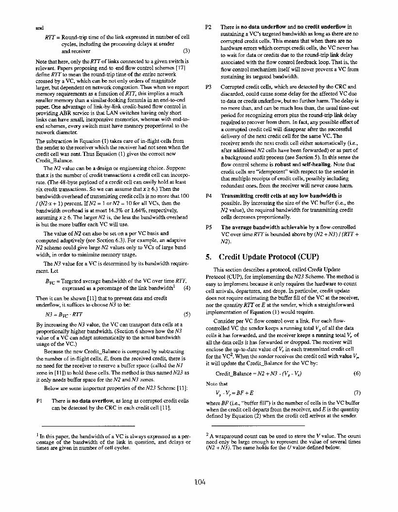
6.3. Receiver-Oriented Adaptation

Adaptive credit allocation can also be done at the receiver. A

receiver-oriented adaptation, described in this section, is natural

for the case where a common buffer pool in a switch is shared by

VCS from multiple input links. Figure 8 depicts such a scenario

the buffer pool at output port p of switch R is shared by four VCS

from two switch S1 and S2. Note that the rezeiver (R) can observe

the bandwidth usage of the VCS from all the senders (S1 and S2).

In contrast, each sender can only observe the bandwidth usage of

those VCS going out from the same sender. Therefore, it is natural

to use receiver-oriented adaptation in this case.

Receiver-Oriented

SI

Figure 8: Receiver-oriented adaptation

The receiver dynamically changes the credit allocation to a VC

based on its relative bandwidth usage of the VC on the outgoing

link. The increase or decrease of the credh allocation will be

reflected by the Vr value (see Section 5) in the next credit cell sent

by the receiver for the VC. That is, V, will increase or decrease in

the same way as the credit allocation.

Suppose that the round-trip times (RZT1 and J?ZT2) of the two

links connecting R to S1 and S2 have different values. Then an

adaptive scheme should allow for adjusting credit allocations

based on the relative bandwidth usage of a VC weighted by the

VC’S RTT. The size of the buffer pool at the receiver should be

related to p . RTT=, where RZT@ is the maximum R7T value

for all the links, and as defined in Section 6, p >1 is a small

constant.

There two important features of the receiver-oriented adapta-

tion:

.

●

As noted above, the size of the buffer pool at the receiver is

related to k?-, independent of the number of input links

sharing the same buffer.

In addition to the N3 adaptation, the N2 value of each VC can

also be adaptive. This works naturally for the receiver-oriented

adaptation as only the receiver needs to use N2 values and thus

can conveniently change them locally as it wishes. For a given

credit allocation of a VC, the allocation can simply be split

between N2 and N3 according to some policy. For example,

N2 can be given to be one half, or some other proportion, of

the allocated credit. This allows only those VCS of large band-

width usages to use large N2 values, so that the bandwidth

overhead of transmitting credit cells can be minimized while

still keeping the total N2 zones of all the VCS relatively small.

In general, an inactive VC can be given an N2 value of 1. The

N2 value will increases as VC’S bandwidth ramps up. Thus the

total allocated memory for all VCS can be as small asP . RTT_ + #l VCS.

The ramp up for the receiver-oriented adaptation over a link

will be delayed by about KIT, compared to the sender-oriented

adaptation. However, for a multiple-hop connection while a VC is

107

ramping upon one link, it can also start ramping up the next link as

soon as data that have caused the ramp up on the fist link begin to

reach the second link. Thus, the total extra delay in the receiver-

oriented adaptation is expected to be only about one RTT ca-re-

sponding to that hop which has the largest RTT value. TMS has

been validated by simulation results, which will be reported in

another paper.

7. Flow-Controlled Statistical Multiplexingfor Minimizing Switch Memory

For the N23 Scheme, or any other similar credh-based flow

control method, the total amount of memory required to allow all

the VCS to reach their desired peak bandwidth can be large, espe-

cially for WANS where propagation delays are large. However if

we allow some (very) small probability of cell loss, then the

memory size can be significantly reduced by statistical multi-

plexing. It will be shown that credit-based flow control will

improve the effectiveness of statistical multiplexing.

We use the notion of “virtual memo~” to describe the concept

of using statistical multiplexing in reducing the size of the “real

memory” of a switch. This is depicted in Figure 9.

D:.Virtual

Memory

Figure 9: “Viial memory” for credh allocation and“real memory” for storing data cells

● VC’S buffer (the N2 and N3 imeas) for supporting credit-based

flow control is allocated from the virtual memory of the

switch.

● Buffer space actually occupied by data cells at any given time

(shaded area) is allocated from the real memory of the switch.

When the real memory is overflowed, data cells will be

dropped. The real memory is sized for low cell loss.

There are advantages of using a virtual memory substantially

larger than the real memory. These include fast bandwidth ramp up

in adaptive credit allocation, and increased number of admitted

flow-controlled VCS.

There are reasons to expect that this virtual memory approach

based on statistical multiplexing can be effective. Obviously, an

inactive VC with no data cells to forward will not consume any

real memory. Even an active VC, un&r a non-congestion situation,

will occupy at most one cell in the real memory at any time, inde-

pendently of the VC’S bandwidth As long as data is flowing on the

links, then one RTT worth of data is included in the N2 + N3

values, but never occupies switch memory.

It is well known that statistical multiplexing is expected to be

effective when a large number of VCS of relatively small average

bandwidths and small bursts share a real memory. Using the N23

credit-based flow control, bursts will be txmn&d by N2 + N3 cells.

Using N2 = 10 and a relatively small value for N3, we can ensure

that the carried traffic will have small bursts and therefore the use

of statistical multiplexing in minimizing memoty will work well.

The is validated by the simulation results in the next section.

In summary, suppose that there are A flow controlled VCS, and

they use the same N2 and N3 values. If the flow control mechanism

needs to guarantee that there is never any cell loss due to conges-

tion, then M must be at least A*(N2+N3). However, if some non-

zero probability of cell loss is acceptable, then M can be much

smaller than A*(N2+N3).

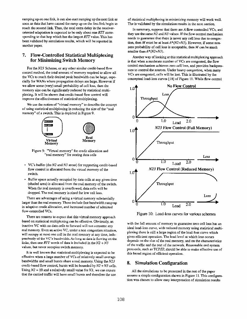
Another way of looking at this statistical multiplexing approach

is that when a moderate number of VCS are congested, the flow

control mechanism achieves zero cell loss, and provides backpres-

sure to control the sources. Under heavy congestion when many

VCS are congested, cells will be lost- This is illustrated by the

conceptual load-loss curves [18] of Figure 11. While flow control

1.04No F1OW Control

Loss

Throughput

o0 1.0

t

N23 Flow Control (Full Memory)1.0

Loss

ad 2:0 ~

t

N23 Flow Control (Reduced Memory)1.0

1/ Throughput

LQss 1

1:0 Load 2:0

Figure 10 Load-loss curves for various schemes

with the full amount of memory to guarantee zero cell loss has an

ideal load-loss curve, with reduced memo~ using statistical muh.i-

plexing there is still a large region of the load-loss curve which

gives efficient operation. The load level at which loss occursdepends on the size of the real memory, and on the chmacteristics

of the traffic and the rest of the network. Reasonable end system

protocols, such as TCP/IP, should be able to make effective use of

this broad region of efficient operation.

8. Simulation Configuration

All the simulations to be presented in the rest of the paper

assume a simple configuration shown in Figure 11. This configura-

tion was chosen to allow easy interpretation of simulation results

108

and also it is sufficiently general to cover most of the key issues we

want to address.

There areN VCS originating from some number of source hosts

(indicated by shaded rectangles) and passing through two switches

(indicated by shaded circles). There are several VCS on each input

port of Switch-1, and all the VCS depart from the same output port

of Switch 2. Thus congestion is expected at this output port. (In

Figure 11, each solid bar indicates a switch input or output port.)

All the VCS will share the same M-cell memory in Switch-1.

(Switch-1 is referred to as “the switch” in the rest of the paper,

unless otherwise stated explicitly.) We assume a simple output

buffered switch where VCS can be individually scheduled and

accessed at each output port

Host

8.1.

Al.

A2.

8.2.

B:

Figure 11: Simulation configuration

Simulation Assumptions

The N VCS have identical load involving B-cd

bursts. The inter-burst times are exponentially

distributed such that the average offered load of

each VC is (ToM Offered Load)/iV of the link

bandwidth.

The switch memory, shared by all the N VCS, has

M = ~N*B cells where ~ <1 is the “Memory

Reduction Factor” due to statistical multiplexing.

(A goal of a statistical multiplexing method in

minimizing M would be to achieve a small value

of ~ for a wide range of B and N values.)

RTZ

F

L:M

Notations

VC burst size (# cells)

Link round-trip time between each host and

the switch (# cells)Total offered load (% of the link bandwidth of the switch

output port)

Cell loss rate (%)Size of switch memory (# cells)

MMU Maximum observed memory usage (# cells) for a giventraftic load over the length of the simulation

N Number of VCSE Simulated time (# cell cycles)

a Memory Reduction Factor

9. Simulation Suite A: Performance as aFunction of Allocated Credit Size

The Suite A simulations show how throughput, delay, and loss

rates are affected by the N3 parameter. Clearly, a VC with larger

N3 will have higher throughput and lower delay than a VC with

lower N3, because it will be blocked less often due to lack of

credit.

In the following two series of simulations, with 100 and 200

VCS respectively, we show the loss rate, memory usage, average

delay, and link utilization as a function of the VC’S N3 value.

We also take different approaches to showing memory require-

ments in the two series. Simulation Al shows the number of

dropped cells with a fixed size memory. Simulation A2 shows the

maximum memory required so that no cells were dropped over the

simulation interval. Note that in both simulations, 4,800 cell times

of the delay is due to link propagation time.

9.1. Simulation Al (Figure 12)

B (VC burst size)= 172RTT (Link round-trip time)= 3,200F (Total offered load)= 95%

M (Switch memory size)= 4096N (Number of VCS) = 100T (Simulated time)= 1,000,000

N2 = 10

25000 — — 100%

20000 , , so%

15000 , , 60%

1000O , , a%

5000 ,

0

Figure 12: Link utilization, # cell delays and # droppedcells as function of N3 values on the horizontal axis

(Simulation Al)

9.2. Simulation A2 (Figure 13)

B (VC burst size)= 172

RIT (Link round-trip time)= 3,200

F (Total offered load)= 95%M (Switch memory size)= Unlimited

N (Number of VCS) = 200T (Simulated Time)= 1,000,000N2 = 10

10. Simulation Suite B: Comparing FC AndNon FC Statistical Multiplexing

The suite B simulations show the memory use characteristics of

flow-controlled (FC) vs. non flow-controlled (non FC) traffic.

Simulating switches with unlimited memory, we report two values:

minimum memory such that the loss rate with FC was very low

(no cells lost in a 1 million cell simulation), and minimum memory

to achieve low cell loss without flow control.

109

25000, 1100%

20000 , , 80%

15000 , , 60%

1000O ,

5000 ~

Figure 13: Link utilization, # cell delays, and maximummemory usage (MMU) as function of N3 values

(Simulation A2)

10.1. Theory to Be Validated

T1. For the same N and 1?,flow control can sigrtifi-

cantly lower B while achieving the same

throughput and the same rate of cell loss.

10.2. Simulation B1

B (VC burst size)= 172 (corresponding to an 8K-Byteblock in a datagrarn protocol such as NFS)

RIT (Link round-trip time)= 3,200(approximately one-way 225km for the OC-12 rate,or 900km for the OC-3 rate)

F (Tottd offered load)= 95%N (Number of VCS) = 100T (Simulated time)= 1,000,000

N2 = 10

N3 = 48 (hence peak rate is 1.5% of link rate)In the both FC and non-FC cases the average utilization of the

output port was about 95~0.

FC Non FC

3250 Cells o Small (i.e., L<. 1%)

~ Value

2% > 19~o

Table 1: Comparing cell loss rates for FC and non FC

statistical multiplexing at two memory sizes

(Simulation B 1)

Note that the above results of simulation B 1 summarized in

Table 1 validate theory T1 in Section 10.1.

By analysis one can expect that for multi-switch configurations

flow control is just as effective as for the single-switch case, as far

as minimizing switch memory by statistical multiplexing is

concerned. This has been confirmed by our multi-switch simula-

tions, which are not reported here.

11. Simulation Suite C: Adaptive CreditAllocation

The suite C simulations shows the effect of the adaptive N3

algorithm, described in Section 6, on delay and memory usage.

11.1. Simulation Cl

1?(VC burst size)= 172

RZT (Link round-trip time)= 3,200F (Total offered load)= 95%

M (Switch memory size)= Unlimited

N (Number of VCS) = 100T (Simulated time)= 1,000,000 cell periods

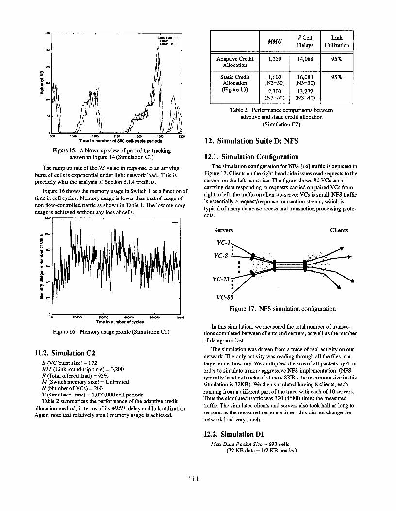
Figure 14 plots the N3 values of a representative VC against

iterations of the adaptive credit algorithm - one iteration is 500 cell

cycles. The N3 values change rapidly to adapt to offered load

changes. Note that changes of the N3 vahtes at Switch-1 closely

track those at the source host, and those at Switch-2 closely track

those at Switch-1. (The three traces are so close that they almost

coincide in Figure 14.) A blown up version of part of this tracking

is shown in Figure 15.

s iOst—!.l —! -2 ....-

Ill,.0 2W *O WO MO 1~ 1?00 14S0 1600 1800 .-.

Time in number of WJ-cell-cycle periods

Figure 14: Changes of the N3 at the source hos~Switch-1 and Switch-2 track each other closely

(Simulation Cl)

Notice that the N3 values of consecutive switches track each

other with only a short delay. As can be seen in Figure 15, a switch

lags behind the switch upstream by no more than 5,000 cell cycles.

‘Ilk reaction time is only a little more than a roundtrip time (3,200

here).

The peak N3 reached in response to a burst is about equal to the

burst size (172) in most cases. Figure 14 shows that it never

exceeds twice the burst size for this particular set of parameters.

The adaptive N3 can reach values much higher than would be

practical for a statically defined N3. This allows the switch to clear

the burst through as quickly as possible, reducing delay.

110

I2.&emd —

!Awa.l ---awldl .2...

‘m )1

1

Figure 15: A blown up view of part of the trackingshown in Figure 14 (Simulation Cl )

The ramp up rate of the N3 value in response to an arriving

burst of cells is exponential under light network load., This is

precisely what the analysis of Section 6.1.4 predicts.

Figure 16 shows the memory usage in Switch- 1 as a function of

time in cell cycles. Memory usage is lower than that of usage of

non flow-controlled traffic as shown in Table 1. The low memory

usage is achieved without any loss of cells.Im

I—

01 Io ZoumO - m 8x1000 1e+cm

Tm in numb of cycles

Flgore 16: Memory usage profile (Simulation Cl)

11.2. Simulation C2

B (VC burst size)= 172RTT (Link round-hip time)= 3,200F (Total offered load)= 95%

M (Switch memory size)= UnlimitedN (Number of VCS) = 200T (Simulated time). 1,000,000 cell periods

Table 2 summarizes (he performance of the adaptive credit

allocation method, in terms of its MkfU, delay and link ut~lzation.

Again, note that relatively small memory usage is achieved.

MMU# Cell Link

Delays Utilization

Adaptive Credit 1,150 14,088 95%Allocation

~Table 2 Performance comparisons between

adaptive and static credh allocation

(Simulation C2)

12. Simulation Suite D: NFS

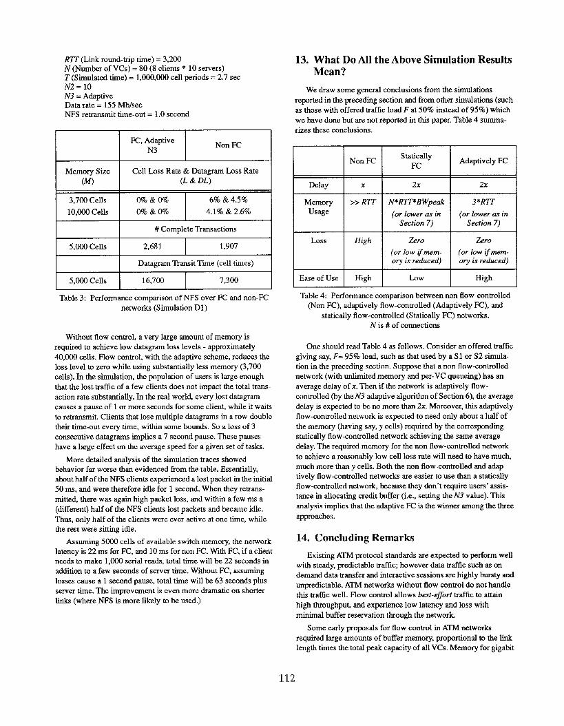
12.1. Simulation Configuration

The simulation configuration for NFS [16] traffic is depicted in

Figure 17. Clients on the right-hand side issues read requests to the

servers on the left-hand side. The figore shows 80 VCS each

carrying data responding to requests carried on paired VCS from

right to lefg the traffic on client-to-server VCS is small. NFS traffic

is essentially a requestiesponse transaction stream, which is

typical of many database access and transaction processing proto-

cols.

Servers Clients

Vc-1,

VC-8

VC-73

VC-80

Figure 17: NFS simulation configuration

In this simulation, we measured the total number of transac-

tions completed between clients and servers, as well as the number

of datagrsms lost.

The simulation was driven horn a trace of real activity on our

network. The only activity was reading through all the files in a

large home duectory. We multiplied the size of all packets by 4, in

order to simulate a more aggressive NFS implementation. (NFS

typically handles blocks of at most 8KB - the maximum size in this

simulation is 32KB). We then simulated having 8 clients, each

running from a different pmt of the trace with each of 10 servers.

Thus the simulated traffic was 320 (4*80) times the measured

traffic. The simulated clients and servers also took half as long to

respond as the measured response time - this did not change the

network load very much.

12.2. Simulation D1

Max Data Packet Size = 693 cells(32 KB data+ 1/2 KB header)

111

I

R7T (Link round-trip time)= 3,200N (Number of VCS) = 80 (8 clients * 10 servers)T (Simulated time)= 1,000,000 cell periods= 2.7 swN2 = 10

N3 = AdaptiveData rate = 155 Mb/see

NFS retransmit time-out= 1.0 second

I FC, Adaptive

N3 I Non FC II

Memory Size Cell Loss Rate & Datagratn Loss Rate

(M) (L& DL)

3,700 Cells o% & (370 6% & 4.5%

10,000 Cells (w. &o% 4.1% & 2.6%

# Complete Transactions

I 5,000ceIk I 2,681 I 1,907I

Datagram Transit Time (cell times)

5,000 Cells 16,700 7,300

Table 3: Performance comparison of NFS over FC and non-FC

networks (Simulation D 1)

Without flow control, a very large amount of memory is

required to achieve low datagram loss levels - approximately

40,000 cells. Flow con~ol, with the adaptive scheme, reduces the

loss level to zero while using substantially less memory (3,700

cells). In the simulation, the population of users is large enough

that the lost traffic of a few clients does not impact the total trsm-

action rate substantially. In the real world every lost datagram

causes a pause of 1 or more seconds for some client, while it waits

to retransmit. Clients that lose multiple datagrams in a row double

their time-out every time, within some bounds. So a loss of 3

consecutive datagrams implies a 7 second pause. These pauses

have a lsrge effect on the average speed for a given set of tasks.

More detailed analysis of the simulation traces showed

behavior far worse than evidenced from the table. Essentially,

about half of the NFS clients experienced a lost packet in the initial

50 ms, and were therefore idle for 1 second. When they retrans-

mitted, there was again high packet loss, and within a few ms a

(different) half of the NFS clients lost packets and became idle.

Thus, only half of the clients were ever active at one time, while

the rest were sitting idle.

Assuming 5000 cells of available switch memory, the network

latency is 22 ms for FC, and 10 ms for non FC. With FC, if a client

needs to make 1,000 serial reads, total time will be 22 seconds in

addition to a few seconds of server time. Without FC, assuming

losses cause a 1 second pause, total time will be 63 seconds plus

server time. The improvement is even more dramatic on shorter

links (where NFS is more likely to be used.)

13. What Do All the Above Simulation ResultsMean?

We draw some general conclusions horn the simulations

reported in the preceding section and from other simulations (such

as those with offered traflic load Fat 50% instead of 95~o) which

we have done but are not reported in this paper. Table 4 summar-

izes these conclusions.

INon FC I statically

FC I Adaptively FC

1 I 1

I Delay x 2x 2x

Memory >> RTT N*RTT*BWpeak 3*RW

Usage (or lower as in (or lower as inSection 7) Sectwn 7)

Loss High Zero Zero

(or low ifmem- (or lbw ifmem-ory is reduced) ory is reduced)

I Ease of Use I High I Low I High

Table 4: Performance comparison between non flow-con~olled

(Non FC), adaptively flow-controlled (Adaptively FC), and

statically flow-controlled (Statically FC) networks.

N is # of connections

One should read Table 4 as follows. Consider an offered traffic

giving say, F= %~. load, such as that used by a S1 or S2 sittmla-

tion in the preceding section. Suppse that a non flow-controlled

network (with unlimited memory and per-VC queueing) has an

average delay of x. Then if the network is adaptively flow-

controlled (by the N3 adaptive algorithm of Section 6), the average

delay is ex~cted to be no more than 2x. Moreover, this adaptively

flow-controlled network is expected to need only about a half of

the memory (having say, y cells) required by the correspding

statically flow-controlled network achieving the same average

delay. The required memory for the non flow-mntrolled network

to achieve a reasonably low cell loss rate will need to have much,

much more than y cells. Both the non flow-controlled and adap-

tively flow-controlled networks are easier to use than a statically

flow-con~olled network, because they don’t require users’ assis-

tance in allocating credit buffer (i.e., setting the N3 value). This

analysis implies that the adaptive FC is the winner among the three

approaches.

14. Concluding Remarks

Existing ATM protocol standards are expected to perform well

with steady, predictable traftic; however data traffic such as on

demand data transfer and interactive sessions are highly bursty and

unpredictable. ATM networks without flow control do not handle

thii traffic well. Flow control allows best-ejj$ort traffic to attain

high throttghptt~ and experience low latency and loss with

mirtiial buffer reservation through the network

Some early propsals for flow con~ol in ATM networks

required large amounts of buffer memory, proportional to the link

length times the total peak capacity of all VCS. Memory for gigabit

112

ATM switches can be expensive due to the high bandwidth

involved. Although these flow control proposals, without

employing techniques of this paper, could be practical for LANs

with small link propagation delays, the large memory requirements

created many difficulties for ATM WANS:

● Hosts had to make accurate estimates of how much bandwidth

they would require, in order to request an appropriate credit

buffer size (i.e., wme N3-equivalent value).

● Idle VCS consumed significant switch resources. Attempting

to deactivate idle VCS imposed significant protocol overheads

on the hosts and switches.

● Traffic requiring large peak bandwidths but with low average

bandwidth (X Window System connections, for example) used

network resources very inefficiently

The results reported in this paper improve this situation in two

ways. First, we have shown that much smaller memories can

provide zero or low loss rates through statistical multiplexing - in

fact the use of flow control cart reduce total switch memory

requirements for bursty traffic.

Second, the adaptive credit allocation protocol eliminates the

need for hosts to estimate their traffic requirements, and allows

highly bursty, variable traffic sources to use network resources

efficiently. Am cart be as simple and efficient for computer

communications as TCP over IF networks.

our initial flow-controlled switches designs required substan-

tial hardware support for credit mattagement. Many aspects of

credit cell management required sub-microsecond processing. The

CUP method described in this paper, however, is designed with a

sof~are implementation in mind.

A “Credit Card” added as an overlay on a conventional ATM

switch can run the credk protocol in software. Because the N2 is

used to reduce the credit processing, the software only needs to

process about 1 event for every tens of cells of flow-controlled

traffic (see Section 4), requiring perhaps 10 memory references

Our reference architecture, used for all simulations reported

here, is designed so that delays in processing by the software will

only result in a slight degradation in total throughput of flow-

controlled cells, but will never produce incorrect behavior such as

dropping cells.

In our reference implementation, all the machinery required for

flow control runs only at the link rate (not a multiple thereof, as do

many parts of ATM switches). It requires only the following

switch features above the features common to any ATM switch

●

✎

✎

A Credit Card, containing a fast microcontroller, capable of

sending and receiving cells at the nominal link rate. It might

replace a port cssd in a backplane-style switch, and it can be

the same engine that runs connection setup processing.

Egress, ingress, and drop counters for each VC, readable by

the Credh Card. (Some ATM switches already have these

counters).

Per-VC credit counters on each port card, which are decre-

mented when a cell is sent. The scheduler must not send cells

for VCS with no credit.

● Per-VC N2 counters on each port card which are decremented

for every cell sent. When a counter reaches zero, the ID

number of that VC is enqueued in a FIFO, readable by the

Credit Card. This ID signals the Credit Card to send a credit

cell.

The adaptive credit allocation protocol used in our simulations

is still at art early stage of development. We suspect that many

interesting algorithms will be developed that can irtqxove perfor-

mance substantially over the results we have shown. This effort

will be aided by the nature of CUP:

.

.

The implementation of the tdgorithtn as softsvare allows easy

experimentation and sophisticated algorithms.

The basic credit cell prirtitive, and the lost data cell recovery

message, are the ordy protocol elemerm required between

switches. Simple and easy to standardwe, the CUP protocol

will allow switch manufacturers to develop new and better

adaptive algorithms to optimize throughput of their switches.

CUP makes a uniform flow control possible on both LAN and

WAN ATM networks, and is simple enough that it can be easily

standardized for heterogeneous networks. We have shown that

using flow control can reduce memory requirements, and adaptive

credit allocation can reduce them still further, while also sirttpli-

fying connection setup. We think CUP is the right foundation on

which to provide best-effort capabilities in ATM networks.

References

[1]

[2]

[3]

[4]

[5]

[6]

[7]

[8]

[9]

ATM Forum, “ATM User-Network Interface Specification;Version 3.0, Prentice Hall, Englewood Cliffs, New Jersey,1993.

“ISDN - Core Aspects of Frame Protocol for Use with Frame

Relay Bearer Service,” ANSI T1.618-1991.

“High-Performance Parallel Interface - Mechanical, Elec-

trical and Signaling Protocol Specification (HIPPI-PH)”,

ANSI X3.183-1991.

S. Borkar, R. Cohn, G. Cox, T. Gross, H. T. Kung, M. Lam,M. Levine, M. Wne, C. Peterson, J. Susman, J. Sutton, J.

Urbanski and J. Webb, “Integrating Systolic and Memory

Communication in iWarp,” Conference Proceedings of the17th Annual International Symposium on Computer Architec-ture, Seattle, Washington, June 1990, pp. 70-81.

A. Demers, S. Keshav, and S. Shenker, “Analysis and Sirmtla-tion of a Fair Queueing Algorithm,” Proc. SIGCOMM ’89

Symposium on Communications Architectures and Protocols,

pp.1-12.

H. J. Fowler and W. E. I-eland, “Local Area Network TrafficChmacteristics, with Implications for Broadband NetworkCongestion ?vlartagement,” IEEE J. on Selected Areas in

Cornmurt., vol. 9, no. 7, pp. 1139-1149, Sep. 1991.

M. W. Garrett, “Statistical Analysis of a Long Trace of Vari-able Bit Rate Video Traffic,” Chapter IV of Ph.D. Thesis,

Columbia University, 1993.

V. Jacobson, “Congestion Avoidance and Control,” Proc.SIGCOMM ’88 Symposium on Communications Architec-

tures and Protocols, Aug. 1988.

M. G. H. Katevcnis, “Fast Switching and Fair Control ofCongested Flow in Broadband Networks,” IEEE J. on

113

Selected Areas in Commun., vol. SAC-5, no. 8, pp. 1315-

1326, Oct. 1987.

[10] H. T. Kung, “Gigabit Local Area Networks: A SystemsPerspective,” IEEE Communications Magazine, 30 (1992),

pp. 79-89.

[11] H. T. Kung and A. Chapman, ‘“The FCVC (Flow-ControlledVitua.1 Channels) Proposal for ATM Networks,” Version 2.0,

1993. A summary appears in Proc. 1993 International Con$on Network Protocols, San Francisco, California, October 19-22, 1993, pp. 116-127. (Postscript files of this and otherrelated papers by rhe authors and their colleagues are avail-able via anonymous lTP horn virtual.harvard. edudpubihtk.)

[12] H.T. Kung, R. Morris, T. Charuhas, and D. Lin, “Use of Link-by-Link Flow Control in Maximizing ATM Networks Perfor-

mance: Simulation Results,” Proc. IEEE Hot InterconnectsSymposium, ’93 Palo Alto, Cahfomi% Aug. 1993.

[13] W. E. Leland, M. S. Taqqu, W. Wilinger and D. V. Wilson,

“On the Self-Similar Nature of Ethernet Traffic,” Proc.SIGCOMM ’93 Symposium on Communications Architec-tures and Protocols, 1993.

[14] A. Parekh and R. G. Gallager, “Generalized Processor

Sharing Approach to Flow Control in Integrated Services

Networks - The Mukiple Node Case,” IEEE INFOCOh4 ’93,San Francisco, Mar. 1993.

[15] K.K. Ramakrishnan and R. JairL “ABinary Feedback

Scheme for Congestion Avoidance in Computer Networks,”

ACM Transactions on Computer Systems, Vol. 8, No. 2, pp.

158-181, May 1990.

[16] Sun Microsystems. “NFS: Network File System Protocol

Specification, “ RFC 1094, Mm 1988.

[17] N. Ym and M. G. Hluchyj, “On Closed-Loop Rate Control forATM Cell Relay Networks,” submitted to IEEE Infocom

1994.

[18] C.L. Williamson D.L. Cheriton, “Load-Loss Curves: Supportfor Rate-Based Congestion Control in High-Speed Datagrarn

Networks,”, Proc. SIGCOMM ’91 Symposium on Communi-

cations Architectures and Protocols, pp. 17-28.

114