Microeconomic Evidence of Creative Destruction in Industrial and Developing Countries

By Eric Bartelsman, John Haltiwanger and Stefano Scarpetta1

This version: October 2004

Abstract

In this paper we provide an analysis of the process of creative destruction across 24 countriesand 2-digit industries over the past decade. We rely on a newly assembled dataset that draws from different micro data sources (business registers, census, or representative enterprisesurveys). The novelty of our approach is in the harmonisation of firm level data across countries, which enables international comparisons and the identification of country-specific factors as opposed to sectoral and time effects. All countries display a massive reallocation of resources, with the entry and exit of many firms in all markets, the failure of many newcomers and the expansion of successful ones. This process of creative destruction affects productivity directly,by reallocating resources towards more productive uses, but also indirectly through the effects of increased market contestability. There are also large differences across groups of countries. While entry and exit rates are fairly similar across industrial countries, post entry performance differs markedly between Europe and the U.S., a potential indication of the importance of barriers to firm growth as opposed to barriers to entry. Transition economies show an even more impressive process of creative destruction and, amongst them, those that have progressed the most towards a market economy show better outcomes from this process. Finally, Mexico shows large firm dynamics with many new firms entering the battle but also many failing rapidly, whileArgentina resembles more of Continental Europe with smaller flows and less impressive post-entry growth of successful firms.

JEL classification: L11, G33, D92,

Keywords: entry, exit, survival, firm size, productivity, micro data

1. Respectively: Free University Amsterdam and Tinbergen Institute; University of Maryland, U.S.Census Bureau, and NBER; The World Bank. We are grateful to the World Bank for financialsupport of this project and to Karin Bouwmeester, Helena Schweiger and Victor Sulla forexcellent research assistance. The views expressed in this paper are those of the authors and should not be held to represent those of the World Bank or its countries.

1

1. Introduction

A rapidly growing number of studies provide evidence of heterogeneity in firm behavior, even within narrowly-defined industries or markets (see Caves, 1998; Bartelsman andDoms, 2000; and Ahn, 2000 for surveys). In all countries studied, there is evidence that the population of firms undergo significant changes over time, both through resource reallocationbetween existing firms and the process of firm entry and exit. . For the study of productivity, therole of within-firm productivity growth vs. the productivity growth induced by the reallocation of resources from less productive to more productive businesses has been the focus of much recentresearch (see, e.g., Olley and Pakes (1996), Griliches and Regev (1995) and Foster, Haltiwanger and Krizan (2001,2002)). The impact of changing patterns of international trade on an economyis increasingly viewed through these lenses, with evolving trade relations changing the marketstructure and mix of businesses (e.g. Helpman, Melitz, and Yeaple, 2004). At the same time, the substantial churning of firms, along with the reallocation of labor across continuing firms, impliesthat workers and firms incur in significant search and other adjustment costs (see, e.g., Mortensen and Pissarides, 1999; and Caballero and Hammour, 2000). As such, the efficiency of an economyin dealing with such reallocation is important not only for the productivity dynamics of the economy, but also for the dynamics of the labor market and in particular of unemployment. For all of these reasons, firm-level dynamics appear to be crucial for the relative success of developedeconomies and also for the trajectories of transition and emerging economies as they develop and open up markets (see Eslava et. al., 2004; Roberts and Tybout, 1997; Aw, Chung and Roberts,2002; and Brown and Earle, 2004 for studies on Latin America, East Asia and transition economies, respectively).

Much useful work on these issues has proceeded on a country-by-country basis, using firm-level datasets for a specific country. But there also is a clear interest and need to combinedata from multiple countries. This allows in principle an assessment of how much of the observed dynamism at the micro level is due to industry-specific technological factors and marketcharacteristics, and how much is the results of different institutional and policy settings thatinfluence firm behavior and competitive forces in each market. In this paper, we do not specifically address the role of policy and institutions. Instead, we conduct exploratory dataanalysis exercises of the panel dataset exploiting the variation across countries, industries and time. The dataset, constructed through ‘distributed micro-data analysis’ as described in detail in Bartelsman, Scarpetta, and Haltiwanger (2004), includes indicators built up from (confidential) micro-level sources available to researchers in each of the countries included.2

We present evidence on the process of creative destruction in a selection of industrialized and developing economies. We focus on the distribution of firm-size over time, the frequency and size of firm entry and exit, the evolution of the (size) distribution of firms by entry-cohort. Further, we analyze the sources of productivity growth at the industry and aggregatelevels. We look at the contribution of firm entry and exit to productivity growth as well as at the contribution coming from the reallocation of resources across existing firm. Overall, we provide a comprehensive picture of the magnitude, characteristics and effectiveness of the creative

2. The approach to collecting and constructing harmonized firm-level data in this project differsfrom projects like the ICA project that use the same survey instrument in a number of countries.A discussion of the advantages and disadvantages of the alternative approaches as well as the relationship on key findings from the ICA dataset vs. the type of firm-level data used here isprovided in Haltiwanger and Schweiger (2004). Recent papers that have used the ICA data tostudy firm performance include Bastos and Nasir (2004), Dollar et. al. (2003), Hallward-Driemeier et al. (2003).

2

destruction process and, by exploiting the different dimensions of our data, we make the firstattempt at understanding the sources of the observed variations across countries and industries.Our country dataset includes 24 economies over a period covering most of the past decade; ten industrial countries, five Central and Eastern European countries in transition, and nine emergingeconomies in Latin America and East Asia. These countries differ significantly along differentdimensions including the underlying economic conditions and the policy and institutionalsettings.

The remainder of the paper is organized as follows. In Section 2, we briefly review the recent theory on the reasons behind firms’ heterogeneity and the importance of experimentationand learning by doing. In this section, we also discuss how policy and institutional settings mayinfluence firm heterogeneity. We argue that different policy settings may influence firm behavior in multiple ways and that several firm-level indicators are needed to assess how the differentpolicy choices ultimately affect economic efficiency. In Section 3, we provide a brief description of the data for 24 industrial, transition and emerging economies. We then turn to the empiricalevidence. In Section 4 we first present the distribution of firms by size; we then document the magnitude and key features of firm dynamics (entry and exit of firms) and, finally, we study postentry performance of different cohorts of new firms. In Section 5 we analyze the effectiveness ofcreative destruction for productivity growth. We distinguish between the productivitycontribution coming from the process of creative destruction (entry and exit of firms) to thatstemming from within-firm efficiency improvements and reallocation of resources acrossincumbents. In the final section, we draw some preliminary conclusions and propose a researchagenda to start exploring the links between policy and firm dynamics.

2. Firm heterogeneity, market structure and institutions

Stylized Facts

Over the past two decades, evidence has mounted suggesting sizable heterogeneity offirms across different interrelated dimensions, size, growth, market shares, life cycle etc. In particular, some regularities have been found in the growing empirical literature, including (see e.g. Sutton, 1997; Pakes and Ericson, 1998, Geroski, 1995 for surveys):3

1. Size and growth: The probability of survival tends to increase with firm (or plant) size; but, conditional on survival, the proportional rate of growth of a firm is decreasing in size (see Evans 1987a, 1987b; Dunne et al. 1988, 1989).

2. The firm life cycle: For any given size of firm, the proportional rate of growth is smaller the older the firm, but its survival probability is greater (see Foster et al. 2001; and the survey ofpost entry performance of firms in the International Journal of Industrial Organization,1995).

3. Shakeouts: The number of producers in a given market tends first to rise to a peak, and later to fall to some lower level. Entry rates tend to be higher for more recent industries but tendto decline as the industry matures (Klepper and Graddy, 1990; Klepper and Simons, 1993; Geroski, 1995).

3. Amongst others, see Aghion and Howitt (1992) and Caballero and Hammour (1994, 1996). Foster, Haltiwanger and Krizan (2001), Caves (1998) and Bartelsman and Doms (2000) offerfurther discussion of this literature.

3

4. Churning: There is a high pace of the reallocation of outputs and inputs across businesses that (i) is largely within narrowly defined sectors; (ii) differs substantially across sectors andfirm characteristics (e.g., much more churning amongst young and small businesses);and (iii)where entry and exit of businesses account for a substantial fraction of the variation and thepositive correlation between gross entry rates and gross exit rates across industries helps account for the differences in churning rates across sectors (e.g. Geroski, 1995, Ahn, 2000and Davis and Haltiwanger, 1999 for surveys of the literature).

5. Reallocation and Productivity: The pattern of reallocation is far from random. In well-developed market economies, the evidence is overwhelming that the pattern of reallocation is productivity enhancing. Accounting exercises show that a large fraction oftotal factor productivity and labor productivity growth at the industry level is accounted for by the reallocation of outputs and inputs from less productive to more productive businesses (see e.g. Olley and Pakes, 1996, Griliches and Regev, 1995, and Foster, Haltiwanger andKrizan, 2001, 2002)..

What are firms so heterogeneous?

These statistical regularities depict a story whereby entrant firms start business with a different initial size reflecting differences in their own perceived ability. Because of the inherent uncertainty in their potentials, even an entrant who is very successful, ex post, tends to begin witha smaller size at the initial stage of his life. This provides an explanation why small and youngsurvivors show rapid growth. Competition continuously separates winners and losers with unsuccessful firms exiting the market relatively rapidly, and successful survivors growing andadapting. The accumulation of experience and assets, in turn, strengthens survivors and lowersthe likelihood of failure.

Several theories have been developed to explain these observed patterns of firmdynamics survival and growth. They generally relate to the process of ‘creative destruction’(usually ascribed to Joseph Schumpeter). The distinguishing element of Schumpeter’s theory from ‘standard’ theories of firm behavior is that it recognizes heterogeneity amongst producers and that the continual shift in the composition of the population of firms through entry, exit,expansion and contraction is essential in developing and creating new processes, products andmarkets.

The first two regularities are consistent with one class of models of firm learningprocess, the passive learning model of Jovanovic (1982). In his model, a sequence of firms that do not know their own potential profitability enters the market. Only after entry does the firmstart to learn about the distribution of its own profitability based on noisy information from realized profits. By continually updating such learning, the firm decides to expand, contract, or toexit. One of the main implications of this model is that smaller and younger firms should havehigher and more variable growth rates.

Cabral (1995 and 2003) offers an alternative theoretical explanation for the observednegative relation between firm size and growth (the so called Gibrat’s law). His model assumesthat firms must incur a sunk cost in building production capacity. Since small entrants have a higher probability of exit than large firms, it is optimal for them to invest more gradually, andthus experience higher growth rates if successful, than larger entrants. Cabral also suggests thatfinancial constraints are an alternative for sunkness of capacity and technology investment. Since cash constraints are expected to be less binding after start up, cash constrained start-ups should expect higher-than-average growth rates.

4

Jovanovic and MacDonald (1994) propose a model that is consistent with the observedshakeout of firms as product markets mature. They postulate that at the beginning firms all use a common technology, but over time a new technology emerges which offers low unit costs buthigher level of output per firm. The transition to the new technology involves a shakeout of first generation firms, and the survival of a smaller number of firms which employ the new larger-scale technology. Klepper (1996) combines a stochastic growth process for firms who enter by developing some new products, with the idea that each firm spends some fixed amount to lower its unit costs. Assuming some imperfection in capital markets and inertia in sales, larger firmswill invest more on fixed costs for product innovation, and over time tend to displace smallerfirms generating the shakeout.

The presence of high turbulence in most markets is consistent with the active learning model developed by Ericson and Pakes (1995).4 In their model, a firm explores its economic environment actively and invests to enhance its profitability under competitive pressure from bothwithin and outside the industry. Its potential and actual profitability changes over time in response to the stochastic outcomes of the firm’s own investment, and those of other actors in the same market. The firm grows if successful, shrinks or exits if unsuccessful.

Vintage models of technological change also offer possible explanations for theobserved regularities in firm dynamics and performance. These models stress that new technology is often embodied in new capital which often requires a retooling process in existingplants (see e.g. Solow, 1960; Cooper, Haltiwanger and Power, 1997). Related to this idea aremodels (e.g. Caballero and Hammour, 1994; Mortensen and Pissarides, 1994; Campbell, 1997)that emphasize the potential role of entry and exit: if new technology can be better harnessed bynew firms, productivity growth will be dependent upon the entry of new units of production that displace outpaced establishments. Moreover, the existence of sunk costs implies that new firmsusing the “state-of-the-art” production technology coexist with older and less productive firms generating the observed heterogeneity.

In this paper, we look at harmonized firm-level data for several industrial, transition and developing countries to seek confirmation of the statistical regularities highlighted in previous studies and to assess the possible sources of firm heterogeneity exploiting cross sectoral and well as cross-country variations. As such, this is the first paper, to our knowledge, to exploit a cross-country sample beyond industrialized countries.

The Role of Market Structure and Institutions

It is tempting at first glance to hypothesize that countries -- and/or sectors -- where thecreative destructive process is distorted in some manner will have less churning and lowerproductivity levels and productivity growth rates. Indeed, it is not hard to take extreme versions of the models discussed in the prior section and generate just this prediction. That is, makingentry and exit (and adjustment more generally) prohibitively costly via distorted market structureand institutions will lead to a reduced pace of churning and lower productivity (see, e.g., Davisand Haltiwanger, 1999 for the illustration of this prediction in a calibration exercise using an extreme example where all reallocation is shutdown). Taken literally, this prediction can be tested by examining the variation by country, sector and year in our harmonized data and relating

4. Various empirical papers have attempted to identify passive and active learning processes. Forexample, using US data, Pakes and Ericson (1998) claim that manufacturing firms are moreconsistent with the active learning model whilst retailing firms are more consistent with thepassive learning model.

5

such variation to country, sector and year variations in institutions. Even more simply, the immediate temptation is to test this prediction implicitly by examining the rank ordering of firm turnover and productivity dynamics across countries and to match that rank ordering up withpriors about the rank ordering of market structure and institutions across countries.

However, further reflections suggest that the predictions regarding distortions in marketstructure and institutions are in fact not so clear. The reason is that distortions may affect the reallocation dynamics on different margins in a variety of ways. For example, artificially highbarriers to entry will lead to reduced firm turnover and to a less efficient allocation of resources.But given the high barrier to entry (and in turn the implied ability of marginal incumbents to increase survival probabilities), the average productivity of entrants will rise while the average productivity of incumbents and exiting businesses will fall. Similar predictions apply to policiesthat subsidize incumbents and/or restrict exit in some fashion. The point is that institutional distortions might yield a larger gap in productivity between entering and exiting businesses.

Alternatively, some types of distortions in market structure and institutions might makethe entry and exit process less rational (i.e., less driven by market fundamentals but more by random factors). Such randomness may be associated with either a higher or lower pace ofchurning. Pure randomness would, in principle, increase the pace of churning but the random factors might be correlated with other factors (e.g., firm size) and thus the impact would be to distort the relationship between churning and such factors with less clear predictions on the overall pace of churning. In any event, such randomness would imply less systematic differences between entering, exiting and incumbent businesses – in the extreme when all entry and exit is random there should be no differences between entering, exiting and incumbent businesses.

Another related problem is that a business climate that encourages more marketexperimentation might have a larger long run contribution but a smaller short run contributionfrom the creative destruction process. That is, the greater market experimentation may beassociated with more risk and uncertainty in the short run so that it is only after the trial and errorprocess of the experimentation has worked its way out (through learning and selection effects)that the productivity payoff is realized. Thus, a business climate that encourages marketexperimentation might have a lower short run contribution from entry and exit but a higher long run contribution from entry and exit.

In short, the gap between the productivity of entering and exiting businesses is not by itself sufficient to gauge the contribution or efficiency of the creative destruction process. In addition, different types of distortions might be acting simultaneously in a country. It might be that different policies act to subsidize incumbents (preferential treatment for incumbents), otherpolicies artificially increase the barriers to entry (poorly functioning financial markets and/orregulatory barriers), while other policies make exit more random for some types of businesses (e.g., poorly functioning financial markets for young and small businesses). As such, there mightbe too little churning on some dimensions and too much on others, the gap between entering andexiting businesses might be too large on some margins and too small on others.

All of these remarks suggest the need for both caution and creativity in using the firm demographic and productivity dynamic statistics that we analyze below. On the one hand,even this brief discussion makes clear that simple cross country comparisons on specific dimensions may be misleading or inadequate. On the other hand, this discussion suggests that creativity needs to be used to examine the connection between the churning and productivitydynamics along multiple dimensions. In like fashion, this discussion helps make clear why it is likely important to exploit variation beyond simple country variation but instead exploit variation

6

on additional dimensions like sector and size using difference-in-differences (e.g., exploiting differences in the cross-industry variation across countries).

As will become clear in our discussion of the data in the next section, limitations in the data in different dimensions across countries and compromises that were made to generate ‘comparable’ data, may hamper analysis of certain questions and generally suggest caution ininterpreting simple cross country differences. We now turn to a discussion of the data.

3. A new dataset of firm-level data from industrial and developing countries

The dataset used in the study was collected in various stages. Most recently, thefirm-level project organized by the World Bank collected indicators for 14 countries (Estonia, Hungary, Latvia, Romania, Slovenia; Argentina, Brazil, Chile, Colombia, Mexico, Venezuela, Indonesia, South Korea and Taiwan.(China)) An earlier OECD study collected indicators based on information on firms from: Canada, Denmark, Germany, Finland, France, Italy, theNetherlands, Portugal, United Kingdom and United States.

These projects made use of a common analytical framework and the data analysis and collection was conducted by active experts in each of the countries.5 The framework involves theharmonization, to the extent possible, of key concepts (e.g. entry, exit, or the definition of the unit of measurement) as well as the definition of common methodologies for studying firm-level data.The methodology for collecting the country/industry/time panel dataset built up from underlyingmicro-level datasets has been referred to as ‘distributed micro-data analysis’ (Bartelsman 2004).A detailed technical description of the dataset may be found in Bartelsman, Haltiwanger and Scarpetta (2004).

The distributed micro-data analysis was conducted for two separate analytical themes.The first set of analyses gathered data relating to firm demographics, such as entry and exit, jobsflows, size distribution and firm survival. The second theme gathered indicators of movements of firms and resources related to productivity, such as productivity contributions of entry/exit and other measures of resource reallocation. The synthetic indicators used in the analysis for these two themes are discussed in details in Box 1.

The analysis of firm demographics is based on business registers, census, social securitydatabases, or employment-based register containing information on both establishments and firms(see Table 1). Data for the analysis of productivity growth come more frequently from businesssurveys. Using these data, time-series indicators on firm demographics were generated for

5. In addition to the authors of this paper, the researchers involved in the distributed micro-dataanalysis network for the various projects are: John Baldwin (Canada); Tor Erickson (Denmark);Seppo Laaksonen, Mika Maliranta, and Satu Nurmi (Finland); Bruno Crépon and RichardDuhautois (France); Thorsten Schank (Germany); Fabiano Schivardi (Italy); KarinBouwmeester, Ellen Hoogenboom and Robert Sparrow (the Netherlands); Pedro Portugal Dias(Portugal); Ylva Heden (Sweden); Jonathan Haskel, Matthew Barnes, and Ralf Martin (UnitedKingdom); Ron Jarmin and Javier Miranda (United States); Gabriel Sánchez (Argentina), MarcMuendler and Adriana Schor (Brazil), Andrea Repetto (Chile), Maurice Kugler (Colombia and Venezuela), David Kaplan (Mexico), John Earle (Hungary and Romania), Mihails Hazans(Latvia), Raul Eamets and Jaan Maaso (Estonia), Mark Roberts (Korea, Indonesia and Taiwan(China)), Milan Vodopivec (Slovenia).

7

disaggregated sectors for each country. The classification into about 40 sectors (roughly the 2-digit level detail of ISIC Rev3) coincides with the OECD Structural Analysis (STAN) database.6

The other set of indicators in the dataset concerns productivity and its components. The data sources used for the analysis of productivity differ from those used for firm demographics in many countries. For productivity measures, data are needed on output, employment and possiblyother productive inputs such as intermediate materials and capital services. Using these sourcedata, indicators are calculated on labor productivity by industry and year, and on the decomposition of productivity growth into within-firm and reallocation components (see below).

Box 1 Main indicators available in the firm-level database

The use of annual data on firm dynamics implies a significant volatility in the resulting indicators. In orderto limit the possible impact of measurement problems, it was decided to use definitions of continuing,entering and exiting firms on the basis of three (rather than the usual two) time periods. Thus, thetabulations of firm demographics contained the following variables:

Entry: The number of firms entering a given industry in a given year. Also tabulated, where available,was the number of employees in entering firms. Entrant firms (and their employees) were thoseobserved as (out, in, in) the register in time (t – 1, t, t +1).

Exit: The number of firms that leave the register and the number of people employed in these firms.Exiting firms were those observed as (in, in, out) the register in time (t – 1, t, t +1).

One-year firms: The number of firms and employees in those firms that were present in the registerfor only one year. These firms were those observed as (out, in, out) the register in time (t – 1, t, t +1).

Continuing firms: The number of firms and employees that were in the register in a given year, as well as in the previous and subsequent year. These firms were observed as (in, in, in) the register intime (t – 1, t, t +1).

The above indicators were split into 8 firm-size classes including the class of firms withoutemployees.7 The data thus allow detailed comparisons of firm-size distributions between industries andcountries.

Firm survival: available data allow to track entering firms over time, This allows to calculate survivalprobabilities over the initial life of firms and to assess their changes in employment over time.

Decomposition of productivity growth: The database includes different types of productivitydecomposition for manufacturing industries and some service industries. Depending on the availability ofoutput and input measures, productivity data are available in the database with reference to laborproductivity, multifactor productivity using either gross output or value added as the indicator of output(see Bartelsman et al. 2004 for more details). In this paper, the analysis is limited to labor productivity,generally defined as deflated gross output per worker. Firm level nominal values of output are deflated atthe industry level

6. See www.oecd.org/data/stan.htm

7. For the OECD countries there are only 6 groups, with the groups between 1 and 20 combinedand the groups between 100 and 500 combined.

8

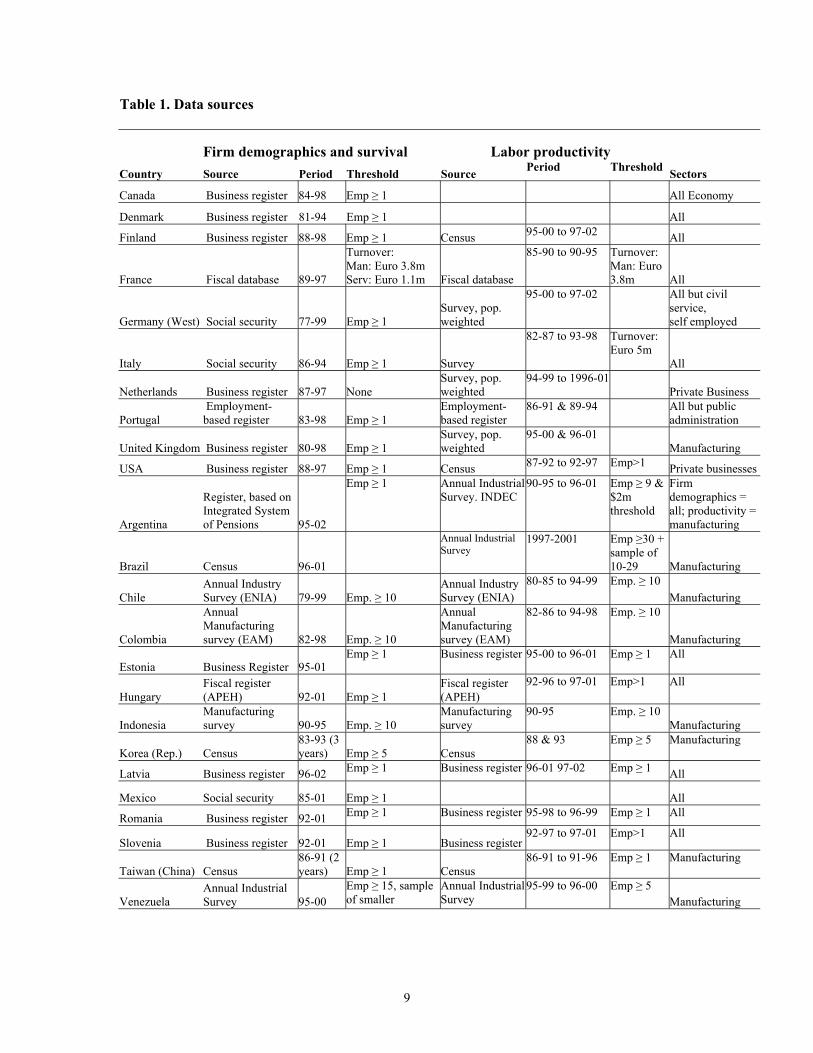
Table 1. Data sources

Firm demographics and survival Labor productivity Country Source Period Threshold Source Period Threshold Sectors

Canada Business register 84-98 Emp 1 All Economy

Denmark Business register 81-94 Emp 1 All

Finland Business register 88-98 Emp 1 Census 95-00 to 97-02 All

France Fiscal database 89-97

Turnover:Man: Euro 3.8mServ: Euro 1.1m Fiscal database

85-90 to 90-95 Turnover:Man: Euro3.8m All

Germany (West) Social security 77-99 Emp 1 Survey, pop.weighted

95-00 to 97-02 All but civilservice,self employed

Italy Social security 86-94 Emp 1 Survey

82-87 to 93-98 Turnover:Euro 5m

All

Netherlands Business register 87-97 NoneSurvey, pop.weighted

94-99 to 1996-01Private Business

Portugal Employment-based register 83-98 Emp 1

Employment-based register

86-91 & 89-94 All but publicadministration

United Kingdom Business register 80-98 Emp 1 Survey, pop.weighted

95-00 & 96-01 Manufacturing

USA Business register 88-97 Emp 1 Census 87-92 to 92-97 Emp>1 Private businesses

Argentina

Register, based onIntegrated Systemof Pensions 95-02

Emp 1 Annual Industrial Survey. INDEC

90-95 to 96-01 Emp 9 & $2mthreshold

Firmdemographics = all; productivity =manufacturing

Brazil Census 96-01

Annual IndustrialSurvey

1997-2001 Emp 30 + sample of 10-29 Manufacturing

ChileAnnual IndustrySurvey (ENIA) 79-99 Emp. 10

Annual IndustrySurvey (ENIA)

80-85 to 94-99 Emp. 10 Manufacturing

Colombia

AnnualManufacturingsurvey (EAM) 82-98 Emp. 10

AnnualManufacturingsurvey (EAM)

82-86 to 94-98 Emp. 10

Manufacturing

Estonia Business Register 95-01Emp 1 Business register 95-00 to 96-01 Emp 1 All

HungaryFiscal register(APEH) 92-01 Emp 1

Fiscal register(APEH)

92-96 to 97-01 Emp>1 All

IndonesiaManufacturingsurvey 90-95 Emp. 10

Manufacturingsurvey

90-95 Emp. 10 Manufacturing

Korea (Rep.) Census83-93 (3 years) Emp 5 Census

88 & 93 Emp 5 Manufacturing

Latvia Business register 96-02 Emp 1 Business register 96-01 97-02 Emp 1 All

Mexico Social security 85-01 Emp 1 All

Romania Business register 92-01 Emp 1 Business register 95-98 to 96-99 Emp 1 All

Slovenia Business register 92-01 Emp 1 Business register92-97 to 97-01 Emp>1 All

Taiwan (China) Census86-91 (2 years) Emp 1 Census

86-91 to 91-96 Emp 1 Manufacturing

VenezuelaAnnual Industrial Survey 95-00

Emp 15, sampleof smaller

Annual Industrial Survey

95-99 to 96-00 Emp 5 Manufacturing

9

4. Assessing the process of creative destruction

The distribution of firms by size: sectoral specialization or framework conditions

The first step in our analysis of creative destruction is to look at the distribution of firm by size across countries and industries. Firm size is an important dimension in our analysis for several reasons. As discussed above, small firms seem to be affected by greater churning, but also have greater potential for expansion. Thus, a distribution of firms skewed towards smallunits may imply higher entry and exit, but also greater post entry growth of successful firms.Alternatively, it may point to a sectoral specialization of the given country towards newerindustries, where churning tends to be larger and more firms experiment with differenttechnologies. However, as for all our firm-level indicators, any observed difference in one single indicator – like firm size -- cannot, per se, be taken to indicate differences in the magnitude or characteristics of creative destruction. The distribution of firm by size is likely to be influencedby the overall dimension of the internal market – especially for non-tradeables – as well as thebusiness environment in which firms operate that can discourage firm expansion (see below). So, the analysis of firm size should be taken as one of the aspects that together with the others on firmdemographics and the productivity decomposition will enable to identify a coherent story aboutcross-country differences in creative destruction.

It should be stressed at the outset that our analysis is affected by the different thresholdsused on firm size. For most countries the data cover all firms with at least one employee. But the cutoff size is 5 employees in South Korea and Venezuela (with a random sample of smaller),8 10employees in Chile, Colombia and Indonesia. Second, even amongst the countries for which data cover all firms with at least one employee, data may be at the establishment level instead of theplant level, and the definition of both may vary across countries. Third, data for some countries are based on other selection criteria, which might induce some bias in the results which cannot bedetermined a priori (e.g. in France data exclude firms with a turnover below a given threshold).Finally, from a sectoral perspective, community services and utilities are more difficult tocompare, given the important role of the public sector, whose coverage changes from country to country, and of regulation in these sectors.

Table 2 suggests that in all countries the population of firms is dominated by microunits (with less than 20 employees).9 They account for at least 80 per cent of the total firmpopulation. Their share in total employment is much lower and ranges from less than 15 percentin some transition economies (e.g. Romania) -- which still reflects the presence of large (formerlyor still) state-owned firms inherited from the central plan period -- to less than 20 percent in the United States and around 30 per cent or more in some small European economies.10

8. However, the enterprise survey in Venezuela is representative of all firms with at least 15employees, and only includes a random sample of firms below this threshold. In our analysis,we have used the data for Venezuela with reference to firms with 20+ employees, given the lackof coverage for the lover size classes.

9. For proper comparability, the Table excludes all countries for which the size threshold is 5 or 10employees instead of one.

10. The Table reports the share of firms with fewer than 20 employees over the total number offirms or total employment for the countries for which we have all firms with at least 1 employee.

10

Table 2. Small firms across broad sectors and countries, 1990s (firms with fewer than 20 employees as a percentage of total)

Totaleconomy

Non-AgricultureBusinessSector (1) Manufacturing

Totalservices

Totaleconomy

Non-AgricultureBusinessSector (1) Manufacturing

Totalservices

Industrial countriesDenmark 91.3 89.5 76.6 92.3 32.7 31.1 17.6 35.0France 82.1 82.3 77.9 82.0 15.9 16.0 19.9 13.6Italy 93.8 93.8 88.6 96.0 35.9 39.6 31.3 36.4Netherlands 96.3 96.5 88.3 97.1 31.8 36.8 18.3 32.9Finland 93.6 92.7 85.4 95.3 29.5 32.7 13.5 39.1West Germany 89.6 85.8 83.3 0.0 25.8 23.8 16.6 0.0Portugal 89.2 88.9 75.3 93.8 32.2 31.4 18.9 42.9UK 81.3 12.4USA 88.0 88.0 72.6 88.7 18.4 19.3 6.7 19.9Latin AmericaBrazil 82.4 17.7Mexico 90.1 90.0 82.8 92.2 23.2 24.5 13.9 28.5Argentina 90.0 89.4 82.1 91.2 27.7 27.7 21.3 27.7Transition economiesSlovenia 87.7 88.0 71.6 93.1 13.4 13.5 5.1 26.0Hungary 84.4 85.5 71.1 90.8 16.0 16.4 8.8 23.6Estonia 80.6 81.3 64.6 87.1 22.8 22.6 11.5 34.2Latvia 87.7 87.7 87.8 87.6 24.7 24.8 26.9 24.2Romania 90.9 91.5 77.1 95.6 12.9 12.8 4.2 31.6East AsiaKorea2 57.0 11.1Taiwan 82.5 26.6* Share of Employment with less than 20 employees(1) This aggregates excludes agriculture (ISIC 1-5) and community services (ISIC3: 75-79)(2) In Korea, data cover firms with 5 or more employees.

Firms Employment*

Average firm size in aggregate manufacturing or business services in some countries may largely result from a specialization towards industries with a small efficient scale. To assessthe role of sectoral specialization versus within sector differences we need a more disaggregatedanalysis based on a shift-and-share decomposition. The idea behind this technique is to determinehow much of the overall deviation of average size from a given benchmark (in our case the cross-country average) is due to country specialization in sectors with different underlyingtechnological and size characteristics and how much to the fact that average size within sectors tends to be different from that of the benchmark. For example, it could be that overall larger size of manufacturing in the United States is mostly due to the fact that the United States has aproductive structure specialized in sectors with large size. The decomposition exploits the following identity:

i ijijj ss , where js is the average firm size in manufacturing in country

j, sij is the average firm size in sub-sector i and ij is the share of firms in sub-sector i with respect to the total number of firms in manufacturing. Define now s as the overall mean in manufacturing across countries and i as the share of overall number of firms in sub-sector j.Then the difference between country j and overall mean can be decomposed as follows:

i iijiiji iiiijiii iji iii ijijj sssssssss ))(()()(

= + s + s [1]

The first term accounts for differences in the sectoral composition of firms, the second for cross-country differences in firm size within each sector and the last an interaction term,

11

which can be interpreted loosely as an indicator of covariance: if it is positive, size and sectoralcompositions deviate from the benchmark in the same direction.

The decomposition (Table 3) suggests that within sector differences generally play the most important role in explaining differences in overall size across countries: this component is much larger (in absolute terms) that the sectoral composition in many countries.11 The within-industry size component is particularly large in the United States, confirming the idea that a larger internal market tends to promote larger firms, but also in some transition economies (Sloveniaand especially Romania) where some very large firms of the central-plan period have survivedduring the transition. However, the sectoral composition also play an important role – similar to the within sector component – in some small European countries such as Denmark and Portugal but also in a relatively larger country like France and an emerging economy like Mexico. Theseresults suggest that both the size structure and the sectoral composition should be controlled for when analyzing firms dynamics and its effects on aggregate performance.

Table 3. Shift and share analysis of the determinants of firm size

CountrySectoral

composition

AverageSize ofFirms

Interactionbetween sectoralcomp. and size Total

Denmark 0.14 -0.03 -0.09 0.01France 0.08 -0.05 -0.05 -0.02Italy -0.02 -0.17 -0.01 -0.20Netherlands 0.01 -0.13 -0.04 -0.16Finland -0.02 -0.05 -0.02 -0.09Portugal -0.05 -0.04 0.02 -0.07UK -0.01 -0.02 -0.03 -0.06USA 0.00 0.42 -0.07 0.34Canada 0.01 0.03 -0.02 0.01Brazil 0.00 -0.08 -0.01 -0.09Mexico 0.06 -0.06 -0.02 -0.02Argentina 0.04 -0.14 -0.02 -0.12Slovenia 0.01 0.30 -0.07 0.24Hungary 0.01 0.14 -0.02 0.12Estonia -0.03 0.07 0.02 0.06Latvia -0.03 -0.20 0.04 -0.20Romania 0.08 0.97 -0.36 0.68Korea 0.04 0.12 0.02 0.18Taiwan 0.03 -0.14 -0.03 -0.14The Total represents the percentage deviation of average size from the cross-country average:the other columns decompose the total into sub-components

contribution coming from differences in:

The decomposition also suggests that the sectoral composition and differences withinsectors are not highly correlated: the interaction term is negative in most cases, and the sign of the sectoral composition and within sector terms is equal in only a few cases. These results do not support the hypothesis that if a country has an institutional setting that favors a certain size structure, say large firms, it is also characterized both by large firms within sector and a sectoralspecialization tilted towards productions naturally characterized by large firms (Davis and Henrekson, 1999).

11. In a sensitivity analysis, we have also replicated the decomposition for the sample of OECDcountries and the non-OECD countries (including also Hungary and Mexico) separately. Theresults are broadly unchanged in the two sub-samples. Moreover, we have replicated thedecomposition at a finer level of sectoral disaggregation and again the results are broadlyunchanged.

12

It is also interesting to look at the dispersion of firm by size within each sector of the economy and to see whether cross-country differences in the dispersion differ across sectors ofthe economy. Table 4 presents coefficient of variation of firm size, normalized by the overall cross-country coefficient of variation.12 If technological factors were predominant in determiningthe heterogeneity of firm size across countries, we should find that the values in the countrycolumns in Table 3 to be concentrated around one. If, on the contrary, the size differences wereexplained mainly by national factors inducing a consistent bias within sectors, then we would expect the countries with an overall value above (below) the average (i.e. in the “Total” category)to be characterized by values generally above (below) one in the sub-sectors. The first elementemerging from the table is that there are clear sectoral patterns which persist across countries. Service sector activities display greater within-industry dispersion in firm size. This is due to thehigher degree of aggregation of most service sectors compared with manufacturing and to the factthat in most service industries small businesses coexist with large multi-plant enterprises. Withinmanufacturing, high-tech industries (electrical equipment, motor vehicles) have a greater dispersion in firm size than other more traditional manufacturing activities.

From a country perspective, industrial economies seem to have a greater dispersion infirm size, within each sector, than the other countries. And within the industrial countries, the United States show a much larger dispersion in firm size, even controlling for the greater averagesize of firms: in total manufacturing the dispersion in the US is double that in the average ofindustrial countries (even controlling for differences in average size) and the differences are evenlarger in some high-tech industries such as those related to the information and communicationtechnology (ICT). Amongst transition economies, the transport sector still accounts for much ofthe overall variation being characterized by the presence of old state-owned firms together with new private (and generally smaller) ventures, while in the emerging economies of Latin Americaand especially East Asia the within-sector dispersion in firm size tend to be smaller than in theindustrial countries. Still, it is interesting that every country but Finland has at least one sector with greater dispersion than the cross-country average and every country but the U.S. has at least one sector (and typically many) with less dispersion than the cross-country average.

All in all, overall differences in average firm size are largely driven by within-sectordifferences, although in some countries sectoral specialization also plays a significant role. Smaller countries tend to have a size distribution skewed towards smaller firms, but the average size of firms as well as the dispersion within and across countries do not map precisely with theoverall dimension of the domestic market. The United States tend to have larger firms and wider dispersion within most industries. Other industrial countries, including France, UK, Portugal, also have relatively larger shares of large firms, but not necessarily large dispersion in firm sizewithin industries. Significant differences are also found across emerging and transition economies. While some common patterns can be identified amongst transition economies and can be easily linked to remaining elements of the central plan period, no single factor can bebrought to explain the observed cross-country differences in the other countries. Overall, these results point to the possible influence of differences in business environment conditions in shaping firm characteristics and the degree of heterogeneity of firms in the economy and further encourage us to continue our journey into the firm level analysis.

12. We use the coefficient of variation because the dispersion of size across industries or countries isnot independent from the average size: sectors (or countries) with larger size also tend to displayhigher standard deviations.

13

Table 4 Within-industry coefficient of variation of firm size(as a ratio to cross-country sectoral average)

cross-countryaverage Mexico Slovenia Hungary Korea Taiwan Estonia Brazil Latvia Romania Argentina

SectorsTotal economy 12.4 0.94 0.52 1.09 0.45 0.47 0.48 0.63 0.66 1.60 0.77Agriculture, Hunting, Forestry And Fishing 6.3 1.46 0.47 0.38 0.39 0.86 0.62Mining And Quarrying 5.7 0.71 0.60 0.56 0.84 1.62 0.39 0.67total manufacturing 7.5 0.78 0.49 0.66 0.74 0.77 0.40 1.04 0.64 1.29 0.68Food Products, Beverages And Tobacco 5.8 1.08 0.33 0.56 0.56 2.40 0.39 1.56 1.18 0.94Textiles, Textile Products, Leather And Footwear 4.0 1.06 0.89 0.68 1.06 0.83 0.63 1.74 0.91 1.17Wood And Products Of Wood And Cork 3.2 1.02 0.81 0.92 1.09 1.07 0.63 1.07 1.23 1.28Publishing, Printing And Reproduction Of Recorded Media 5.9 0.64 0.73 0.71 0.46 0.74 0.37 0.99 0.62 2.23 0.62Coke, Refined Petroleum Products And Nuclear Fuel 2.7 0.63 0.67 1.09 0.97 0.37 1.22 0.30 0.44 1.87Chemicals And Chemical Products 4.4 0.81 0.66 0.96 0.62 1.54 0.54 1.04 0.44 0.93 0.73Rubber And Plastics Products 3.9 0.72 1.34 0.76 0.75 1.13 0.41 0.99 0.50 1.45 0.69Other Non-Metallic Mineral Products 4.2 1.16 0.56 0.70 0.67 0.73 0.42 0.95 0.76 0.80 0.84Basic Metals 4.6 1.19 0.45 0.66 1.11 0.60 0.24 1.75 0.23 0.95 1.57Fabricated Metal Products, Except Machinery And Equipment 3.7 1.12 1.09 0.86 1.11 0.81 0.49 1.23 0.68 1.17 0.73Machinery And Equipment, N.E.C. 4.7 0.67 0.83 0.93 0.65 0.47 1.09 0.87 0.96 0.52Office, Accounting And Computing Machinery 5.3 0.27 0.77 0.49 0.77 0.22 0.79 0.46 0.90 0.25Electrical Machinery And Apparatus, Nec 5.1 0.60 1.35 0.59 1.00 0.62 1.19 0.28 0.70 0.53Radio, Television And Communication Equipment 5.3 0.54 0.67 1.09 0.85 0.84 0.65 0.66 0.85Medical, Precision And Optical Instruments 5.1 0.78 0.79 0.62 0.45 0.49 0.72 0.83 0.62 0.40Motor Vehicles, Trailers And Semi-Trailers 6.6 0.61 0.46 0.57 1.24 0.69 0.37 1.51 0.15 0.49 0.88Other Transport Equipment 5.6 0.79 0.39 0.48 1.33 1.18 0.50 1.24 0.31 0.43 0.63Manufacturing Nec; Recycling 4.1 1.18 0.63 0.63 1.04 0.70 0.79 0.97 0.50 1.04 0.52Electricity, Gas And Water Supply 5.8 1.69 0.26 0.43 1.15 0.52 1.10 0.84Construction 5.0 0.81 0.75 0.67 0.36 0.89 1.09 0.87Services 15.9 0.95 0.64 1.50 0.39 0.55 2.33 0.72---bus sector services 17.1 0.69 0.62 1.42 0.37 0.51 2.23 0.63Wholesale And Retail Trade; Restaurants And Hotels 10.0 0.79 0.55 0.68 0.23 0.47 0.80 1.04Transport And Storage And Communication 15.8 0.64 0.71 1.25 0.44 0.92 1.65 0.76Finance, Insurance, Real Estate And Business Services 11.8 1.19 0.58 0.95 0.25 0.59 0.45 0.73Community Social And Personal Services 9.3 1.92 0.41 0.62 0.23 0.85 1.11 1.25

(as a ratio to cross-country sectoral average)

cross-countryaverage Industrial Other countries France Italy Netherlands Finland Portugal UK USA

SectorsTotal economy 12.4 1.19 0.87 1.69 1.35 0.31 0.68 2.36Agriculture, Hunting, Forestry And Fishing 6.3 1.23 0.81 2.07 0.56 0.48 0.66 1.92Mining And Quarrying 5.7 1.31 0.68 1.26 1.24 0.97 0.31 0.52 3.55total manufacturing 7.5 1.28 0.74 1.04 2.18 1.19 0.49 0.48 1.03 2.83Food Products, Beverages And Tobacco 5.8 1.14 0.85 0.77 1.51 0.86 0.42 0.51 0.82 2.96Textiles, Textile Products, Leather And Footwear 4.0 1.04 0.96 0.67 0.93 0.98 0.55 0.67 1.15 2.32Wood And Products Of Wood And Cork 3.2 1.01 0.99 0.74 0.81 0.87 0.74 0.87 1.18 1.76Publishing, Printing And Reproduction Of Recorded Media 5.9 1.15 0.86 0.59 2.33 0.73 0.66 0.48 0.74 2.46Coke, Refined Petroleum Products And Nuclear Fuel 2.7 1.26 0.77 0.90 1.61 0.89 0.43 0.75 1.53 2.71Chemicals And Chemical Products 4.4 1.24 0.78 1.50 1.11 0.90 0.65 0.66 0.93 2.70Rubber And Plastics Products 3.9 1.11 0.90 0.83 1.82 0.64 0.48 0.49 0.95 2.52Other Non-Metallic Mineral Products 4.2 1.21 0.81 1.03 1.27 0.91 0.59 0.64 1.05 2.81Basic Metals 4.6 1.20 0.84 2.50 1.59 0.72 0.57 0.82 1.63Fabricated Metal Products, Except Machinery And Equipment 3.7 1.04 0.97 0.80 0.91 0.59 0.77 0.96 2.10Machinery And Equipment, N.E.C. 4.7 1.19 0.77 1.02 1.45 0.54 0.68 0.44 1.06 2.88Office, Accounting And Computing Machinery 5.3 1.46 0.53 2.00 1.49 0.58 0.20 1.16 3.63Electrical Machinery And Apparatus, Nec 5.1 1.22 0.74 1.28 1.35 0.78 0.67 1.01 0.99 2.21Radio, Television And Communication Equipment 5.3 1.25 0.69 1.26 1.86 2.21 0.48 0.58 1.38 2.07Medical, Precision And Optical Instruments 5.1 1.27 0.68 1.64 1.06 1.00 0.68 0.65 0.95 2.68Motor Vehicles, Trailers And Semi-Trailers 6.6 1.46 0.58 0.76 2.76 0.94 0.52 0.54 1.47 3.48Other Transport Equipment 5.6 1.44 0.59 1.16 1.74 1.88 1.00 0.70 1.61 2.57Manufacturing Nec; Recycling 4.1 1.19 0.82 1.46 0.77 1.66 0.55 0.51 0.96 2.66Electricity, Gas And Water Supply 5.8 1.09 0.91 0.52 3.14 0.26 0.44 0.73 1.68Construction 5.0 1.21 0.80 1.12 1.39 1.03 0.43 1.07 2.28Services 15.9 0.94 1.05 0.72 1.23 1.21 0.20 0.79 1.83---bus sector services 17.1 1.06 0.95 0.68 1.53 1.48 0.18 0.79 2.17Wholesale And Retail Trade; Restaurants And Hotels 10.0 1.35 0.68 0.93 0.96 1.17 0.21 0.49 4.20Transport And Storage And Communication 15.8 1.10 0.91 0.31 1.85 1.81 0.30 0.82 2.14Finance, Insurance, Real Estate And Business Services 11.8 1.26 0.76 0.89 1.85 2.31 0.23 0.85 2.36Community Social And Personal Services 9.3 0.94 1.04 0.87 1.16 1.03 0.50 1.32

14

The creative destruction process: gross and net firm flows

The second obvious step in our analysis is to look at the magnitude and characteristics of firm creation and destruction. Figure 1 shows entry and exit rates averaged over time (1989onwards) for the business sector and for manufacturing. Confirming one of the key regularities highlighted in the previous literature, the Figure point to a high degree of turbulence in allcountries. Many firms enter and exit most markets every year. Limiting the tabulations to firmswith at least 20 employees to maximize the country coverage, total firm turnover (entry plus exitrates)13 is in between 3-8 per cent in most industrial countries and more than 10 per cent in someof the transition economies. Extending the tabulations to also include micro units (1 to 19 employees) increases total turnover to between one-fifth and one-fourth of all firms. These dataconfirm previous findings that in all countries net entry (entry minus exit) is far less importantthan the gross flows of entry and exit that generate it. This suggests that the entry of new firms in the market is largely driven by a search process rather than augmenting the number of competitors in the market (a point also highlighted by Audretsch, 1995).

There are also interesting differences across countries. In transition economies firm entry largely out-paced firm exit, while more balanced patterns are found in other countries. Obviously this is related to the process of transition and is not sustainable over the longer run. Still it points to the fact that new firms not only displaced obsolete incumbents in the transition phase but alsofilled in new markets which were either nonexistent or poorly populated in the past. This is alsoreflected in the discrepancies between firm entry and exit across firm size. The Latin Americaregion shows a wide variety of experiences: while Mexico, Chile (manufacturing) and Venezuela(manufacturing) show vigorous firm turnover, Colombia and especially Argentina show less turbulence, closer to the values observed in some Continental European countries.

Figure 1. Firm turnover rates in broad sectors, 1990sPanel A: Manufacturing, firms with 20 or more employees

0

1

2

3

4

5

6

7

8

West G

erman

y

Argenti

na

Netherl

ands Ita

lyUSA

Portug

al

Colombia

Estonia

France

Denmark

Latvi

a

Finlan

d UKChil

e

Mex

ico

Sloven

iaBraz

il

Hunga

ry

Roman

ia

Firm Entry Firm Exit

13. The entry rate is defined as the number of new firms divided by the total number of incumbentand entrants firms producing in a given year; the exit rate is defined as the number of firmsexiting the market in a given year divided by the population of origin, i.e. the incumbents in theprevious year.

15

Panel B: Manufacturing, firms with at least 1 employee

0

5

10

15

20

25

West G

erman

y

Argenti

na Italy

Denmark

Netherl

ands

Canad

aUSA

Estonia

France

Finlan

d UK

Portug

al

Mex

icoBraz

il

Hunga

ry

Roman

ia

Sloven

iaLa

tvia

Firm Entry Firm Exit

Panel C: Total business sector, firms 20 or more employees

0

1

2

3

4

5

6

7

8

West G

erman

y

Netherl

ands Ita

ly

France

Portug

al

Estonia

Finlan

dLa

tvia

Argenti

na

Denmark USA

Sloven

ia

Hunga

ry

Mexico

Roman

ia

Firm Entry Firm Exit

Panel D: Total business sector, firms with at least 1 employee

0

5

10

15

20

25

West G

erman

yIta

ly

Denmark

Argenti

na

Netherl

ands

Canad

a

France

Estonia USA

Finlan

d

East G

erman

y

Portug

al

Mex

ico

Roman

ia

Hunga

ry

Sloven

iaLa

tvia

Firm Entry Firm Exit

16

Data for the transition economies clearly show the role of market forces in shaping firmdynamics (Figure 2). At the beginning of their transition to a market economy, both gross and netfirm flows were large compared to industrial and other emerging economies: in some of the transition economies a large fraction of firms were closed down and replaced by new smallventures, and this process accounted for more than 10 percent of total employment. As the transition moved forward gross and especially net flows declined to reach, at the end of the1990s, values fairly close to those observed in other countries.

Figure 2: The evolution of gross and net firm flows in transition economies, business sectorPanel A: Gross firm flows

Slovenia Hungary

Latvia Romania

0.005.00

10.0015.0020.0025.0030.0035.0040.0045.0050.00

92 93 94 95 96 97 98 99

Gross firm flows Net firm flows

0.005.00

10.0015.0020.0025.0030.0035.0040.0045.0050.00

94 95 96 97 98 99

Gross firm flows Net firm flows

0.005.00

10.0015.0020.0025.0030.0035.0040.0045.0050.00

94 95 96 97

Gross firm flows Net firm flows

0.005.00

10.0015.0020.0025.0030.0035.0040.0045.0050.00

94 95 96 97 98 99

Gross firm flows Net firm flows

Panel B: Employment-weighted firm flows Slovenia Hungary

Latvia Romania

-5.00

0.00

5.00

10.00

15.00

20.00

92 93 94 95 96 97 98 99

Gross weighted firm flows Net weighted firm flows

-1.001.003.005.007.009.00

11.0013.0015.00

94 95 96 97 98 99

Gross weighted firm flows Net weighted firm flows

-1.001.003.005.007.009.00

11.0013.0015.00

94 95 96 97

Gross weighted firm flows Net weighted firm flows

-1.001.003.005.007.009.00

11.0013.0015.00

94 95 96 97 98 99

Gross weighted firm flows Net weighted firm flows

17

The high turnover rates amongst small firms suggest that the process of entry and exit of firms involves a proportionally low number of workers. Indeed, including all firms with at least 1 employee suggests that less than 10 per cent of employment is, on average, involved in firm creation and destruction. The difference between un-weighted and employment-weighted firmturnover rates arises from the fact that both entrants and exiting firms are generally smaller than incumbents. For most countries, new firms are only 20 to 60 per cent the average size of incumbents (Figure 3).

Figure 3. Relative firm size of entering and exiting firms relative to the average incumbent

0

0.1

0.2

0.3

0.4

0.5

0.6

0.7

0.8

0.9

Canad

aUSA

Latvi

a

West G

erman

y

Sloven

ia

Roman

ia

Mex

ico

Hunga

ryBraz

il

Argenti

na

Portug

al

Estonia

Netherl

ands UK

France Ita

ly

Denmark

East G

erman

y

Finlan

d

Manufacturing Business Sector

The small size of entrants relative to the average incumbents is driven by different factors across countries.

o In Canada and especially the United States the small relative size of entrant it reflectsboth the large size of incumbents (see above) and the small average size of entrants compared to that in most other countries (in the United States, about 2.5 employees in thetotal economy and about 5 in manufacturing). In other words, entrant firms are further away from the efficient size in the United States than in most other countries for whichdata are available. There are a number of different possible explanations for this. First,the larger market of the United States may partly explain the larger average size of incumbents.14 Second, the wider gap between entry size and the minimum efficient size in the United States may reflect economic and institutional factors, e.g. the relatively lowentry and exit costs may increase incentives to start up relatively small businesses. Wewill return to this issue later.

o In the transition economies, new firms are substantially different from most of the existing firms that were drawn from the centrally-planned period. Indeed the net entry offirms (entry rate minus exit rate) is particularly large amongst micro units (20 or fewer

14 . Geographical considerations may also affect the average size of firms: firms with plantsspreading into different US states are recorded as single units, while establishments belonging tothe same firm but located in different EU states are recorded as separate units.

18

employees): during the centrally planned system there were relatively few of these microfirms which however exploded during the transition in most of business service activities.

Turnover rates vary significantly across sectors in each country. Table 5 presents thesectoral gross turnover rates (entry plus exit rates weighted by employment) normalized by theoverall cross-country average. As before, if technological factors were predominant indetermining the heterogeneity of firm dynamics across countries, we should find that the valuesin the country columns of Table 5 are concentrated around one. The first element to report is that the variability of turnover rates for the same industry across countries is comparable in magnitude to that across industry in each country.15 Turnover rates (especially if weighted byemployment) are somewhat higher in the service sector (especially in trade) than in manufacturing.16 However, in most countries, some high-tech industries with rapid technologicalchanges and market experimentation had relatively high entry rates in the 1990s (e.g. office,computing and equipments and radio, TV and communication). Transition, but also emergingeconomies in Latin America tend to have greater firm churning than in the industrial countries, onaverage. This result is dominated by some sector dominated by few firms (e.g. fuel and petroleum) as well as some traditional activity (e.g. construction) but also some high-techindustry exposed to intense competition and FDI (e.g. radio, TV and communication).

It is also interesting to compare entry and exit rates across sectors to test two competingtheories: one hypothesis is that entry and exit rates at the sectoral level are mostly driven by sectoral shocks. Sectors with positive profit shocks will have high entry and sectors with negative profit shocks will have high exit. If sectoral profit shocks are the predominant source of variation, then the cross-sectional correlation between entry and exit rates should be negative.Alternatively, entry and exit rates at the sectoral level might be driven by the within sector creative destruction process. A sector with a high dispersion of idiosyncratic shocks and/or low barriers to entry and exit will exhibit both high entry and high exit rates. If the creativedestruction process is the predominant factor driving entry and exit, then the cross-sectionalcorrelation of entry and exit should be positive.

In most of the industrial countries annual entry and exit rates are generally positivelycorrelated across industries (Table 6), confirming previous evidence (e.g. Geroski, 1991a;Baldwin and Gorecki, 1991). And the correlations are particularly strong when the entry and exitrates are weighted by employment. The table also presents the correlations between the averageentry and exit rates over the 1990s which account for the possibility that industry changes in entryand exit do not occur in the same year. Indeed, the correlations based on the average over the

15. Two sectors stand out as clear outliers: agriculture, where some countries have very highturnover rates in absolute and relative terms; and electricity, gas and water, where turnover is very low in some countries. This latter result is perhaps not surprising given that this industry isoften dominated by public utilities.

16 . In Italy and especially Finland, however, there appears to be only small differences in churningbetween manufacturing and services. In the case of Italy this is particularly evident for theemployment-weighted turnover and likely reflects the small differences in average size of firmsbetween manufacturing and services. For Finland, the high turnover in manufacturing is likelythe result of major restructuring, which took place in the aftermath of the deep recession of the early 1990s. The lower turnover rate in the French service sector compared with that in manufacturing is likely to depend on the existence of a size threshold in the French data, whichtends to be more binding in the service sector than in manufacturing. As an indication, theFrench data also suggest a higher average size of firms in the service sector than in manufacturing, in contrast with all other countries.

19

decade tend to be even stronger. Perhaps not surprisingly, entry and exit rates are loosely or evennegatively correlated in some of the transition economies where traditional manufacturing sectorsare losing ground while new service sectors are expanding and in some emerging economies(Colombia and Venezuela) where, again, rapid structural changes have occurred in the period observed by the data.

These finding suggests that entries and exits are largely part of a creative destructionprocess in which entry and exit reflects within sector reallocation reflecting idiosyncraticdifferences across firms within sectors.17 Taken at face value, there are a few countries withnegative correlations which might reflect a greater role for sectoral profitability shocks in those countries (and/or might reflect measurement error).

Table 5. Gross firm turnover across countries and sectors (employment-weighted flows)

(as a ratio to cross-country sectoral average)

cross-countryaverage Industrial

Othercountries Denmark France Italy Netherlands Finland

WestGermany Portugal UK USA

total economy 8.1 0.95 1.08 1.26 0.86 1.06 1.24 1.47 0.48 1.15 0.86Agriculture, Hunting, Forestry And Fishing 9.4 1.09 0.87 1.45 1.13 0.96 0.75 0.99 1.63 1.24Mining And Quarrying 7.1 0.87 1.21 0.80 1.48 1.40 0.47 1.78 0.13 0.98 0.80Total Manufacturing 7.1 1.00 1.00 1.19 1.45 1.20 1.17 1.67 0.35 1.10 1.58 0.50Food Products, Beverages And Tobacco 6.8 1.08 0.90 1.63 2.21 1.47 1.41 1.34 0.48 1.68 0.34Textiles, Textile Products, Leather And Footwear 8.3 1.02 0.97 1.37 1.34 1.23 1.47 1.30 0.41 1.14 1.47 0.85Wood And Products Of Wood And Cork 9.1 0.92 1.09 1.02 1.14 0.81 0.97 1.18 0.28 1.26 1.63 0.95Publishing, Printing And Reproduction Of Recorded Media 7.6 1.02 0.98 1.03 1.25 0.87 1.14 2.40 0.32 0.99 1.46 0.51Coke, Refined Petroleum Products And Nuclear Fuel 9.5 0.48 1.48 1.74 1.55 0.10 0.44 0.12Chemicals And Chemical Products 4.3 1.13 0.87 0.96 1.98 1.61 1.69 1.98 0.49 1.24 0.41Rubber And Plastics Products 6.3 0.96 1.04 1.06 1.36 0.99 1.52 1.55 0.40 1.31 0.65Other Non-Metallic Mineral Products 6.4 1.08 0.91 1.24 1.34 1.18 1.39 1.98 0.35 1.07 1.67 0.69Basic Metals 6.2 1.08 0.93 1.52 2.28 0.12 1.25 1.58 1.16 0.56Fabricated Metal Products, Except Machinery And Equipment 8.1 0.99 1.01 1.00 1.07 1.42 1.11 1.44 0.59Machinery And Equipment, N.E.C. 7.8 0.87 1.13 0.74 0.96 0.91 0.84 1.29 1.37 0.45Office, Accounting And Computing Machinery 12.5 0.93 1.07 1.13 1.12 1.36 3.96 1.52 0.18Electrical Machinery And Apparatus, Nec 6.8 1.12 0.88 1.21 1.25 1.21 2.26 0.68 1.60 0.42Radio, Television And Communication Equipment 9.0 0.88 1.13 1.11 0.98 0.31 1.08 1.37 1.40 0.43Medical, Precision And Optical Instruments 6.4 1.17 0.85 1.39 1.18 1.14 1.42 0.52 2.18 0.35Motor Vehicles, Trailers And Semi-Trailers 5.2 0.93 1.06 1.09 0.73 2.68 1.65 0.49 1.22 0.25Other Transport Equipment 9.7 1.01 0.99 0.77 1.21 1.59 1.84 1.50 1.37 0.11Manufacturing Nec; Recycling 9.0 0.90 1.10 1.02 1.51 1.00 0.69 1.16 0.40 0.79 1.53 0.72Electricity, Gas And Water Supply 5.7 1.04 0.94 0.18 1.72 5.16 2.96 1.23 0.13 0.02 0.14Construction 11.7 0.87 1.19 1.07 0.96 1.02 0.63 1.26 0.44 0.94 1.03Services 9.1 0.95 1.06 1.16 0.68 0.80 1.19 1.40 1.10 0.83Market Services 9.6 0.96 1.05 1.17 0.64 0.94 1.10 1.27 1.06 0.95Wholesale And Retail Trade; Restaurants And Hotels 10.5 0.91 1.11 1.05 0.78 0.98 0.78 1.07 1.06 0.89Transport And Storage And Communication 7.8 1.07 0.89 0.99 1.07 0.76 1.05 1.79 0.65 2.27 0.72Finance, Insurance, Real Estate And Business Services 9.6 0.96 1.05 1.35 0.51 0.87 1.54 1.30 0.72 1.05Community Social And Personal Services 8.7 0.77 1.24 1.00 0.73 0.60 1.29 1.07 0.53

17. Dunne et al. (1988) suggest that entry and exit rates are correlated with a lag in the UnitedStates. However, even then the entry rate in a given five-year period is positively correlated with exit rates in the following five years. For an extensive discussion on this issue see Caves (1998). Caves also signals that the correlation between entry and exit reverts to negative in early and latephases of products' life cycle,

20

(as a ratio to cross-country sectoral average)

cross-countryaverage Chile Colombia Mexico Slovenia Hungary Estonia Brazil Latvia Romania Argentina

total economy 8.1 1.16 1.08 1.16 1.16 0.91 0.99 1.00Agriculture, Hunting, Forestry And Fishing 9.4 0.79 1.05 0.72 1.20 0.73 0.93Mining And Quarrying 7.1 1.04 1.44 0.77 2.37 0.92 1.45 0.89Total Manufacturing 7.1 1.01 0.77 0.97 1.14 1.23 1.13 1.30 1.01 0.87 0.84Food Products, Beverages And Tobacco 6.8 1.08 0.68 0.85 0.48 1.41 0.95 1.57 0.86 0.89Textiles, Textile Products, Leather And Footwear 8.3 0.80 0.85 1.30 0.70 1.25 0.83 1.44 0.83 0.90Wood And Products Of Wood And Cork 9.1 1.33 1.00 1.24 0.84 1.29 0.96 1.37 0.79 0.89Publishing, Printing And Reproduction Of Recorded Media 7.6 0.82 0.66 1.01 1.24 1.18 0.84 1.33 1.16 0.99 0.81Coke, Refined Petroleum Products And Nuclear Fuel 9.5 0.74 0.27 1.00 6.60 0.02 8.08 0.37 4.58 0.91 0.11Chemicals And Chemical Products 4.3 1.51 0.80 0.80 0.38 0.48 1.17 1.26 0.97 0.81 0.79Rubber And Plastics Products 6.3 1.16 0.77 1.07 1.00 1.64 0.94 1.35 1.44 0.32 0.85Other Non-Metallic Mineral Products 6.4 0.95 0.69 1.02 0.85 1.51 0.88 1.23 1.16 0.30 0.66Basic Metals 6.2 0.69 0.46 0.73 1.56 1.72 0.98 0.71 1.57 0.35 0.76Fabricated Metal Products, Except Machinery And Equipment 8.1 0.85 0.63 1.20 1.31 1.50 0.72 1.16 1.16 0.52 0.91Machinery And Equipment, N.E.C. 7.8 0.77 0.90 2.15 1.12 0.75 0.94 1.15 1.04 0.86Office, Accounting And Computing Machinery 12.5 5.37 0.26 0.31 0.88 0.23 0.60 2.11 0.53 1.31Electrical Machinery And Apparatus, Nec 6.8 0.62 0.85 0.62 0.73 2.95 0.68 1.24 0.55 0.81Radio, Television And Communication Equipment 9.0 4.16 0.52 1.03 0.86 0.73 0.65 0.42 0.26 0.40Medical, Precision And Optical Instruments 6.4 0.69 1.13 0.66 1.00 0.88 1.21 1.07 0.41 0.87Motor Vehicles, Trailers And Semi-Trailers 5.2 0.99 0.81 0.57 2.33 0.82 0.56 1.58 1.53 0.83 0.73Other Transport Equipment 9.7 1.94 0.73 0.69 1.74 1.02 0.23 0.59 0.86 0.18 0.87Manufacturing Nec; Recycling 9.0 0.74 1.10 1.19 1.33 1.34 0.97 1.16 0.84 1.15 1.21Electricity, Gas And Water Supply 5.7 0.28 0.57 0.70 0.76 1.27 2.92 0.64Construction 11.7 2.31 0.72 1.11 0.88 0.60 0.46 1.27Services 9.1 1.08 1.10 1.16 1.10 0.82 1.19 0.90Market Services 9.6 1.18 0.99 1.08 1.04 0.76 1.10 1.04Wholesale And Retail Trade; Restaurants And Hotels 10.5 1.20 0.97 1.37 1.00 0.71 1.27 1.11Transport And Storage And Communication 7.8 1.11 0.96 0.43 0.88 0.78 0.91 0.98Finance, Insurance, Real Estate And Business Services 9.6 1.01 1.09 1.28 1.45 0.85 0.92 0.93Community Social And Personal Services 8.7 0.61 1.99 1.54 1.18 1.00 1.72 0.62

Table 6. Correlation between entry and exit rates across industries, 1990s

Observations =industry*year

Entry/ExitCorrelation

Entry/ExitCorrelation(Weighted)

Observations =industry

Entry/ExitCorrelation

Entry/ExitCorrelation(Weighted)

Denmark 85 0.3731* 0.6687* 17 0.5681* 0.8739*France 132 -0.2449* -0.1025 22 -0.5250* -0.2986Italy 125 0.0976 0.7999* 25 0.1011 0.6894*Netherlands 175 0.3131* 25 0.6702*Finland 175 0.2717* 0.4084* 23 0.2675 0.2413West Germany 130 0.6880* 0.6242* 13 0.7510* 0.7702*East Germany 56 0.0385 0.5599* 14 0.1855 0.7181*Portugal 124 -0.1239 0.5671* 25 0.3526 0.0331UK 105 0.2845* 0.6412* 15 0.4709 0.7389*USA 199 0.8801* 0.8167* 25 0.8132* 0.9513*Canada 168 0.5782* 0.7683* 21 0.8252* 0.9301*Venezuela 16 -0.3306 -0.1726Chile 128 0.6323* 0.5504* 18 0.0947 0.3741Colombia 129 0.0319 0.1595 18 0.4385 0.5527*Brazil 38 0.3472* 0.5068* 19 0.395 0.7880*Mexico 220 0.1882* 0.5441* 20 0.7756* 0.9159*Argentina 100 0.0582 0.4971* 25 0.3973* 0.7432*Slovenia 178 -0.05 0.7680* 25 -0.1602 0.4373*Hungary 145 0.2445* 0.5651* 25 0.1917 0.7793*Estonia 59 0.4977* 0.2874* 24 0.3344 0.4621*Latvia 98 -0.0609 0.1511 24 0.294 0.1772Romania 119 0.0826 0.1209 21 0.6098* 0.4066Correlations are based on a maximum of 25 industries in the business sector.* = Significant at 10% level.

Annual correlations Correlations on time averages

21

The post-entry performance of firms

The evidence provided in the previous section clearly indicates that firm dynamics (theentry and exit of firms) is not necessarily associated with changes in the size of the population of firms or in the number of products in the market but rather with continuous changes in thecharacteristics of firms in each market. In this context, what happens to firms subsequent to their entry seems at least as important as the entry process itself. Understanding the post-entryperformance sheds light on the market selection process that separates successful entrant firmsthat survive and prosper from others that stagnate and eventually exit. We examine the post-entryperformance of firms sequentially: we start by presenting simple survivor functions acrosscountries and main sectors and then move to non-parametric and semi-parametric analyses ofsurvival.

Figure 4 presents non-parametric (graphic) estimates of survivor rates for firms thatentered the market in the late 1980s and1990s. The survivor rate specifies the proportion of firmsfrom a cohort of entrants that still exist at a given age In the figure, the survival rates are averaged over different entry cohorts and do not take into account differences in the industry composition across countries.

Figure 4. Firm survival at different lifetimes, 1990s Panel A: Manufacturing

00.10.20.30.40.50.60.70.80.9

1

Mexico UK

Colombia

Argenti

na USA

Finlan

dIta

lyChil

e

Estonia

France

Netrhe

rland

s

West G

erman

y

Roman

ia

Hunga

ry

Portug

al

Latvi

a

Sloven

ia

age=2 age=4 age=7

22

Panel B: Total business sector

00.10.20.30.40.50.60.70.80.9

1

Mexico

Argenti

na USAIta

ly

Roman

ia

France

West G

erman

y

Finlan

d

Estonia

Hunga

ry

Portug

al

Netrhe

rland

sLa

tvia

Sloven

ia

age=2 age=4 age=7

Looking at cross-country differences in survivor rates, about 10 per cent (Slovenia) to more than 30 per cent (in Mexico) of entering firms fail within the first two years (Figure 4).Conditional on overcoming the initial years, the prospect of firms improves in the subsequentperiod: firms that remain in the business after the first two years have a 40 to 80 per cent chanceof surviving for five more years. Nevertheless, only about 30-50 percent of total entering firms in a given year survive beyond the seventh year in industrial and Latin American countries, while higher survival rates are found in transition economies.

For most countries, the rank ordering of survival is similar whether using a 2-year,4-year or 7-year horizon suggesting that there is an important country effect that impacts the survival function. However, there are a few interesting exceptions. The U.S. has relatively lowsurvival rates at the 2-year horizon but relatively higher survival rates at the 7-year horizon. Thispattern might reflect the relatively rapid cleansing of poorly performing firms in the U.S. In thenext section, we explore the productivity implications of the turnover patterns that we observe across countries and industries.

Table 7 provides details on the survival rates at age four across industries and countries.The structure of the Table is similar to that in Table 4 above: the first column presents thecross-country average survival rate for each industry; the second and third columns report the deviations from this average for industrial and other countries respectively; while the othercolumns present the deviations for each country individually. Notably, the variation across countries is more systematic than that across industries. Across industries, after four yearsbetween 60 and 80 percent of firms survive, while for example the survival rate in office andcomputing equipment deviates from 40 percent below to 40 percent above the cross-countryaverage of 70 percent. We will return to this in the parametric analysis of survival.

23

Table 7. Survival rate (4 years of age) across countries and industries(as a ratio to cross-country sectoral average)

cross-countryaverage Industrial

Othercountries Finland France UK

WestGermany Italy Netherlands Portugal USA

Mining And Quarrying 0.69 1.05 0.94 1.07 0.91 1.14 1.10 1.15 1.11 0.85Total Manufacturing 0.67 1.00 1.00 0.94 1.02 0.79 1.10 1.04 1.07 1.12 0.95Food Products, Beverages And Tobacco 0.69 1.02 0.98 0.92 1.10 0.69 1.10 1.08 1.01 1.35 0.91Textiles, Textile Products, Leather And Footwear 0.59 0.96 1.03 0.95 0.98 0.75 0.99 1.04 1.02 1.14 0.81Wood And Products Of Wood And Cork 0.64 1.04 0.97 0.95 1.10 0.86 1.12 1.09 1.19 1.04 0.99Publishing, Printing And Reproduction Of Recorded Media 0.69 0.98 1.01 0.97 0.92 0.82 1.04 1.03 1.03 1.13 0.94Coke, Refined Petroleum Products And Nuclear Fuel 0.73 1.05 0.96 1.05 1.05 0.67 1.20 1.23 1.13 1.37 0.79Chemicals And Chemical Products 0.69 1.02 0.99 0.89 0.96 0.88 1.09 1.11 1.04 1.14 1.01Rubber And Plastics Products 0.73 0.98 1.01 0.91 0.97 0.96 1.00 1.00 1.06 1.06 0.90Other Non-Metallic Mineral Products 0.68 1.02 0.98 0.96 1.08 0.76 1.11 1.10 1.08 1.16 0.97Basic Metals 0.69 0.99 1.01 0.94 0.85 1.08 1.15 1.01 0.93Fabricated Metal Products, Except Machinery And Equipment 0.69 1.01 0.99 0.95 0.90 1.05 1.08 1.12 1.00Machinery And Equipment, N.E.C. 0.73 1.01 0.99 0.96 1.03 0.70 1.00 1.09 1.29 0.99Office, Accounting And Computing Machinery 0.70 0.88 1.10 0.92 0.61 1.05 1.03 1.13 0.80Electrical Machinery And Apparatus, Nec 0.74 0.93 1.06 0.90 1.01 0.71 1.00 1.00 0.99 0.91Radio, Television And Communication Equipment 0.71 0.92 1.08 0.99 0.86 0.73 1.00 0.91 1.00 0.95Medical, Precision And Optical Instruments 0.77 0.96 1.04 1.03 0.88 0.70 0.92 1.08 1.15 0.95Motor Vehicles, Trailers And Semi-Trailers 0.70 0.99 1.01 0.87 1.03 0.72 1.08 1.05 1.29 0.92Other Transport Equipment 0.65 0.98 1.01 0.78 1.00 0.77 1.05 1.14 1.25 0.95Manufacturing Nec; Recycling 0.66 1.02 0.98 0.93 0.99 0.78 1.14 1.04 1.11 1.29 0.92Electricity, Gas And Water Supply 0.82 1.01 0.99 1.14 0.98 1.01 1.00 0.99 1.01 0.95Construction 0.64 1.07 0.94 1.00 1.00 1.10 1.03 1.18 1.18 0.98Market Services 0.66 1.02 0.98 0.99 0.96 1.01 1.02 1.14 1.09 0.96Wholesale And Retail Trade; Restaurants And Hotels 0.64 1.02 0.98 0.91 1.01 1.02 1.03 1.07 1.12 0.96Transport And Storage And Communication 0.66 0.98 1.02 1.22 1.05 1.00 1.04 1.07 0.45 0.94Finance, Insurance, Real Estate And Business Services 0.70 1.01 0.99 1.01 0.85 1.00 1.01 1.16 1.10 0.95Total non-agricultural business sector 0.65 1.02 0.99 1.00 0.99 0.82 1.05 1.04 1.16 1.13 0.97

(as a ratio to cross-country sectoral average)

cross-countryaverage Industrial

Othercountries Estonia Hungary Latvia Romania Slovenia Argentina Chile Colombia Mexico

Mining And Quarrying 0.69 1.05 0.94 0.49 1.11 0.98 1.40 0.84 0.69Total Manufacturing 0.67 1.00 1.00 1.05 1.10 1.11 1.09 1.22 0.89 1.04 0.87 0.76Food Products, Beverages And Tobacco 0.69 1.02 0.98 1.02 1.03 1.09 1.15 0.86 1.03 0.95 0.80Textiles, Textile Products, Leather And Footwear 0.59 0.96 1.03 1.19 1.21 1.30 1.20 0.91 1.08 0.87 0.80Wood And Products Of Wood And Cork 0.64 1.04 0.97 1.01 1.08 1.04 1.26 0.83 1.13 0.77 0.69Publishing, Printing And Reproduction Of Recorded Media 0.69 0.98 1.01 0.95 1.04 1.08 1.06 1.23 0.93 1.09 1.02 0.77Coke, Refined Petroleum Products And Nuclear Fuel 0.73 1.05 0.96 0.97 1.14 1.37 1.37 0.83 0.93 1.11 0.92Chemicals And Chemical Products 0.69 1.02 0.99 0.95 1.04 1.07 1.09 0.95 1.02 1.00 1.00 0.86Rubber And Plastics Products 0.73 0.98 1.01 1.14 1.10 1.12 1.05 1.20 0.94 1.02 0.90 0.81Other Non-Metallic Mineral Products 0.68 1.02 0.98 1.11 1.04 1.17 1.09 1.22 0.89 0.98 0.83 0.74Basic Metals 0.69 0.99 1.01 0.97 1.35 1.03 1.32 0.90 1.13 0.92 0.78Fabricated Metal Products, Except Machinery And Equipment 0.69 1.01 0.99 1.12 1.12 1.21 1.09 1.27 0.85 1.00 0.82 0.70Machinery And Equipment, N.E.C. 0.73 1.01 0.99 1.01 1.09 0.96 1.03 1.20 0.86 0.97 0.75Office, Accounting And Computing Machinery 0.70 0.88 1.10 1.42 1.16 1.10 1.02 1.22 0.60 1.42 1.42Electrical Machinery And Apparatus, Nec 0.74 0.93 1.06 1.02 1.06 1.05 1.10 1.13 0.93 1.14 0.98Radio, Television And Communication Equipment 0.71 0.92 1.08 0.95 1.07 1.27 1.07 1.22 0.86 1.06 1.04Medical, Precision And Optical Instruments 0.77 0.96 1.04 1.30 1.07 1.15 1.01 1.12 0.99 1.04 0.81Motor Vehicles, Trailers And Semi-Trailers 0.70 0.99 1.01 1.07 1.14 1.43 1.14 1.16 0.95 0.96 0.83 0.81Other Transport Equipment 0.65 0.98 1.01 1.37 1.13 1.43 1.21 1.06 0.83 0.88 0.88 0.76Manufacturing Nec; Recycling 0.66 1.02 0.98 1.05 1.11 1.20 1.11 1.17 0.89 1.07 0.78 0.70Electricity, Gas And Water Supply 0.82 1.01 0.99 0.95 0.98 1.12 1.05 1.06 0.95 0.88Construction 0.64 1.07 0.94 1.16 1.16 1.21 1.17 1.31 0.66 0.32Market Services 0.66 1.02 0.98 1.07 1.06 1.12 0.96 1.19 0.89 0.73Wholesale And Retail Trade; Restaurants And Hotels 0.64 1.02 0.98 1.06 1.07 1.13 0.98 1.20 0.87 0.74Transport And Storage And Communication 0.66 0.98 1.02 1.15 1.11 1.22 1.04 1.14 0.98 0.78Finance, Insurance, Real Estate And Business Services 0.70 1.01 0.99 1.06 1.06 1.13 1.00 1.20 0.91 0.75Total non-agricultural business sector 0.65 1.02 0.99 1.09 1.10 1.15 1.00 1.23 0.88 1.07 0.90 0.67

Each given cohort tends to increase in the initial years because failures are highlyconcentrated amongst its smallest units and because of the significant growth of survivors. These facts are best presented by looking at survival rates expressed in terms of total employment of a

24

given cohort and in terms of gains in average firm size amongst surviving firms (Figures 5 and 6).The time profile of the survivor function expressed in terms of employment is shifted upward andis flatter compared with the survival function of firms, due to the exit of predominantly smaller units. On average employment in a given cohort remains in the 80-120 per cent range of its initiallevel after the first two years of its life.

Figure 6 shows the evolution in average firm size of survivors as they age, corrected for possible changes in entry size of the actual survivors by age. In the Figure the average size ofsurvivors at different duration is compared with that at entry.18 The difference in post-entry behavior of firms in the United States19 compared with the West European countries is partiallydue to the larger gap between the size at entry and the average firm size of incumbents, i.e. there is a greater scope for expansion amongst young ventures in the US markets than in Europe. Inturn, the smaller relative size of entrants, can be taken to indicate a greater degree of experimentation, with firms starting small and, if successful, expanding rapidly to approach the minimum efficient scale.20

Latin American countries also offer a wide range of post-entry performance of firms. Argentina has very limited post-entry expansion of successful firms in manufacturing, while in Mexico selection of small firms is stronger than in all other countries, but post-entry growth of successful firms is also very strong, pointing to a strong market selection process but also strong rewards to successful new firms.

18. Given differences in data collection, the reference average size of entrants is that at duration onefor industrial countries and duration zero for other countries, but excluding firms with zeroemployment. The choice for the industrial countries is dictated by the fact that entrant firmsinclude zero-employee firms. This, however, may represent an over-correction as it eliminates employment growth in firms with positive employment at registration. Earlier estimates(Bartelsman, Scarpetta and Schivardi, 2003) which did not make this correction show largerincrease in surviving firms in some countries (e.g. the United States). In the United States, thetime when the firm is registered and when its employment is recorded differ giving rise to thepossibility that firms are recorded as having zero employees in the entry year and positiveemployment in the second year. However, recent work by Jarmin (2003), shows that even aftercorrecting for the zero-employee problem, the size expansion of entrant firms in the U.S. exceeds that in other industrial countries by a wide margin. The growth in firm size in theensuing years shows that the United States continues to perform much better than other OECD countries.

19. The results for the United States are consistent with the evidence in Audretsch (1995). He foundthat the four-year employment growth amongst surviving firms was about 90 per cent.

20. This greater experimentation of small firms in the US market may also contribute to explain theevidence of a lower than average productivity at entry, as discussed below.

25

Figure 5 Employment-based survival rates at different lifetimes, Total employment, 1990s Panel A: Manufacturing

0

0.2

0.4

0.6

0.8

1

1.2

1.4

1.6

1.8

Netrhe

rland

s

Colombia UK

Finlan

d

Argenti

na

France Ita

lyChil

e

West G

erman

yUSA

Sloven

ia

Portug

al

Roman

ia

Estonia

Hunga

ry

Mexico

Latvi

a

age=2 age=4 age=7

Panel B: Total Business sector

00.20.40.60.8

11.21.41.61.8

Argenti

na

Finlan

d

Netrhe

rland

sUSA

Mexico Ita

ly

France

West G

erman

y

Portug

al

Roman

ia

Sloven

ia

Hunga

ry

Estonia

Latvi

a

age=2 age=4 age=7

Transition economies show a different behavior from most other countries also on firm survival. They tend to show higher survivor rates and large post entry growth of successful firmswhich confirm the hypothesis that new firms enjoyed a period of relatively low marketcontestability especially in new low populated markets. Romania is obviously an outlier amongst transition economies: not only are failure rates higher than in the other countries, but even successful entrants have more limited opportunities of expanding.

26

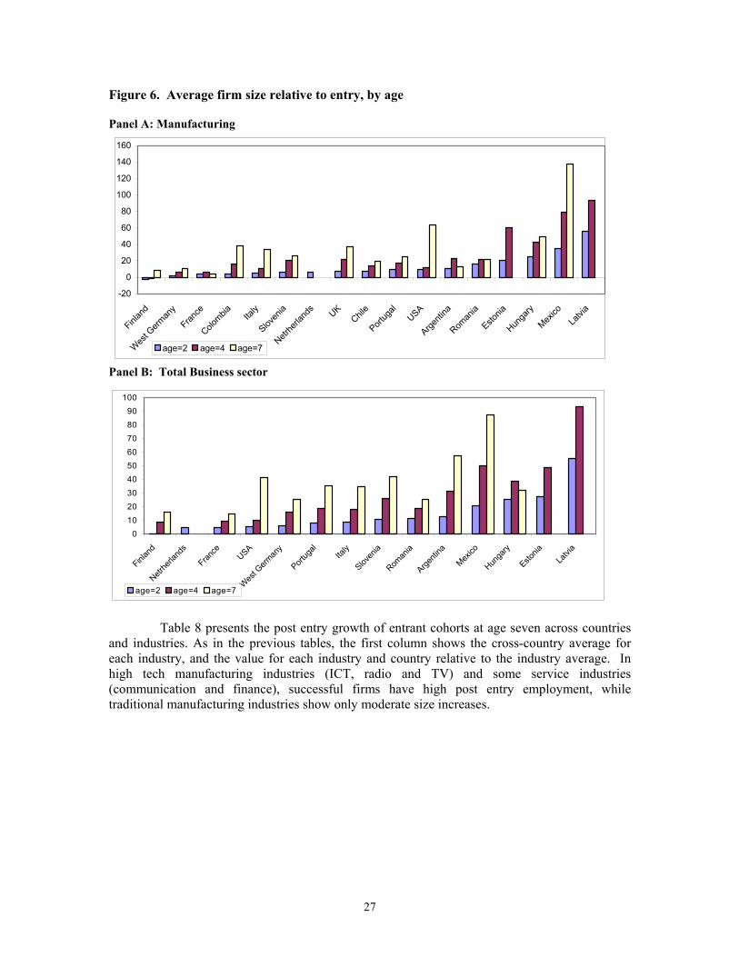
Figure 6. Average firm size relative to entry, by age

Panel A: Manufacturing

-20

0

20

40

60

80

100

120

140

160

Finlan

d

West G

erman

y

France

Colombia Ita

ly

Sloven

ia

Netrhe

rland

s UKChil

e

Portug

alUSA

Argenti

na

Roman

ia

Estonia

Hunga

ry

Mexico

Latvi

a

age=2 age=4 age=7

Panel B: Total Business sector

0102030405060708090

100

Finlan

d

Netrhe

rland

s

France

USA

West G

erman

y

Portug

alIta

ly

Sloven

ia

Roman

ia

Argenti

na

Mexico

Hunga

ry

Estonia

Latvi

a

age=2 age=4 age=7

Table 8 presents the post entry growth of entrant cohorts at age seven across countriesand industries. As in the previous tables, the first column shows the cross-country average for each industry, and the value for each industry and country relative to the industry average. In high tech manufacturing industries (ICT, radio and TV) and some service industries (communication and finance), successful firms have high post entry employment, while traditional manufacturing industries show only moderate size increases.

27

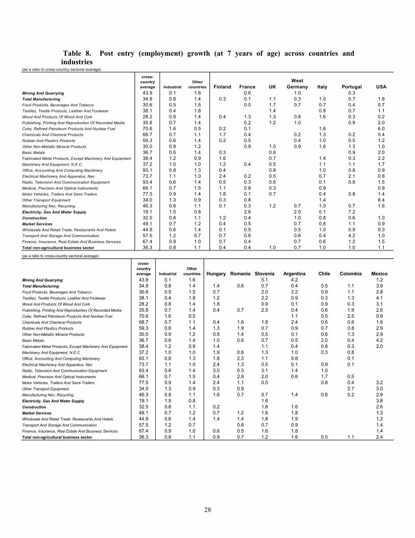
Table 8. Post entry (employment) growth (at 7 years of age) across countries andindustries

(as a ratio to cross-country sectoral average)

cross-countryaverage Industrial

Othercountries Finland France UK

WestGermany Italy Portugal USA

Mining And Quarrying 43.9 0.1 1.6 0.6 1.0 0.3Total Manufacturing 34.9 0.8 1.4 0.3 0.1 1.1 0.3 1.0 0.7 1.8Food Products, Beverages And Tobacco 30.6 0.5 1.5 0.0 1.7 0.7 0.7 0.4 0.7Textiles, Textile Products, Leather And Footwear 38.1 0.4 1.8 1.4 0.8 0.7 1.1Wood And Products Of Wood And Cork 28.2 0.8 1.4 0.4 1.3 1.3 0.8 1.6 0.3 0.2Publishing, Printing And Reproduction Of Recorded Media 35.8 0.7 1.4 0.2 1.2 1.0 0.9 2.0Coke, Refined Petroleum Products And Nuclear Fuel 70.6 1.6 0.5 0.2 0.1 1.6 6.0Chemicals And Chemical Products 68.7 0.7 1.1 1.7 0.4 0.2 1.3 0.2 0.4Rubber And Plastics Products 59.3 0.6 1.4 0.2 0.5 0.4 1.0 0.5 1.2Other Non-Metallic Mineral Products 30.0 0.9 1.2 0.9 1.0 0.9 1.6 1.3 1.0Basic Metals 36.7 0.6 1.4 0.3 0.6 0.9 2.0Fabricated Metal Products, Except Machinery And Equipment 38.4 1.2 0.9 1.6 0.7 1.4 0.3 2.2Machinery And Equipment, N.E.C. 37.2 1.0 1.0 1.2 0.4 0.5 1.1 1.1 1.7Office, Accounting And Computing Machinery 93.1 0.8 1.3 0.4 0.8 1.0 0.8 0.9Electrical Machinery And Apparatus, Nec 73.7 1.1 1.0 2.4 0.2 0.5 0.7 2.1 0.8Radio, Television And Communication Equipment 93.4 0.6 1.4 0.5 0.3 0.6 0.1 0.8 1.5Medical, Precision And Optical Instruments 66.1 0.7 1.5 1.1 0.8 0.3 0.9 0.9Motor Vehicles, Trailers And Semi-Trailers 77.5 0.9 1.4 1.8 0.1 0.7 0.4 0.8 1.4Other Transport Equipment 34.0 1.3 0.9 0.3 0.8 1.4 6.4Manufacturing Nec; Recycling 46.3 0.8 1.1 0.1 0.3 1.2 0.7 1.0 0.7 1.6Electricity, Gas And Water Supply 19.1 1.5 0.8 2.6 2.0 0.1 7.2Construction 32.5 0.8 1.1 1.2 0.4 1.0 0.8 0.6 1.0Market Services 49.1 0.7 1.2 0.4 0.5 0.7 0.8 1.1 0.9Wholesale And Retail Trade; Restaurants And Hotels 44.9 0.6 1.4 0.1 0.5 0.5 1.0 0.9 0.3Transport And Storage And Communication 57.5 1.2 0.7 0.7 0.6 0.6 0.4 4.2 1.0Finance, Insurance, Real Estate And Business Services 67.4 0.9 1.0 0.7 0.4 0.7 0.6 1.2 1.5Total non-agricultural business sector 36.3 0.8 1.1 0.4 0.4 1.0 0.7 1.0 1.0 1.1(as a ratio to cross-country sectoral average)

cross-countryaverage Industrial

Othercountries Hungary Romania Slovenia Argentina Chile Colombia Mexico

Mining And Quarrying 43.9 0.1 1.6 5.1 4.2 1.2Total Manufacturing 34.9 0.8 1.4 1.4 0.6 0.7 0.4 0.5 1.1 3.9Food Products, Beverages And Tobacco 30.6 0.5 1.5 0.7 2.0 2.2 0.9 1.1 2.8Textiles, Textile Products, Leather And Footwear 38.1 0.4 1.8 1.2 2.2 0.9 0.3 1.3 4.1Wood And Products Of Wood And Cork 28.2 0.8 1.4 1.8 0.9 0.1 0.9 0.3 3.1Publishing, Printing And Reproduction Of Recorded Media 35.8 0.7 1.4 0.4 0.7 2.5 0.4 0.6 1.9 2.6Coke, Refined Petroleum Products And Nuclear Fuel 70.6 1.6 0.5 1.1 0.5 2.5 0.9Chemicals And Chemical Products 68.7 0.7 1.1 0.4 1.6 1.8 2.4 0.6 0.6 1.6Rubber And Plastics Products 59.3 0.6 1.4 1.3 1.9 0.7 0.9 0.7 0.8 2.9Other Non-Metallic Mineral Products 30.0 0.9 1.2 0.8 1.4 0.5 0.1 0.6 1.3 2.9Basic Metals 36.7 0.6 1.4 1.0 0.6 0.7 0.5 2.0 0.4 4.2Fabricated Metal Products, Except Machinery And Equipment 38.4 1.2 0.9 1.4 1.1 0.4 0.8 0.3 2.0Machinery And Equipment, N.E.C. 37.2 1.0 1.0 1.9 0.6 1.3 1.0 0.3 0.8Office, Accounting And Computing Machinery 93.1 0.8 1.3 1.8 2.3 1.1 0.8 0.1Electrical Machinery And Apparatus, Nec 73.7 1.1 1.0 2.4 1.3 0.5 0.1 0.9 0.1Radio, Television And Communication Equipment 93.4 0.6 1.4 3.0 0.3 3.1 1.4 1.0Medical, Precision And Optical Instruments 66.1 0.7 1.5 0.4 2.9 2.0 0.6 1.7 0.5Motor Vehicles, Trailers And Semi-Trailers 77.5 0.9 1.4 2.4 1.1 0.5 0.8 0.4 3.2Other Transport Equipment 34.0 1.3 0.9 0.3 0.9 2.7 3.0Manufacturing Nec; Recycling 46.3 0.8 1.1 1.6 0.7 0.7 1.4 0.8 0.2 2.9Electricity, Gas And Water Supply 19.1 1.5 0.8 1.6 3.8Construction 32.5 0.8 1.1 0.2 1.8 1.6 2.6Market Services 49.1 0.7 1.2 0.7 1.2 1.6 1.8 1.3Wholesale And Retail Trade; Restaurants And Hotels 44.9 0.6 1.4 1.4 1.4 1.8 1.9 1.2Transport And Storage And Communication 57.5 1.2 0.7 0.6 0.7 0.9 1.4Finance, Insurance, Real Estate And Business Services 67.4 0.9 1.0 0.6 0.5 1.6 1.8 1.4Total non-agricultural business sector 36.3 0.8 1.1 0.9 0.7 1.2 1.6 0.5 1.1 2.4

28

Controlling for sectoral composition and right-censoring

The survival analysis discussed so far suffers from two problems: i) as in the case of firmsize and firm turnover, differences in sectoral composition are likely to influence the observed cross-country differences in survival rates; and ii) right censoring makes comparisonsproblematic especially for countries for which we have short longitudinal series. In order to compare survival and exit hazards across countries and sectors, and to cope with the right-censoring and other problems in the data (in some countries, non-monotonic survival rates), we complement non-parametric counts with a statistical survival analysis. The survival distributionfunction (SDF) is used to describe the lifespan of the population of interest. The SDF evaluated at t is the probability that an experimental unit from the population will have a lifetime, T, of at least t, that is:

tTtS Pr)( [2]

where S(t) denotes the survival function and T is the lifetime of a randomly selected experimental unit.

Some functions closely related to the SDF are the cumulative distribution function (CDF), the probability density function (PDF) and the hazard function (HF). These are defined as:

)()()(:

)()(:

)(1)(:

tStf

thHF

ttF

tfPDF

tStFCDF

[3]

We have used the Cox’ proportional hazard model to study firm survival. This modelassumes a p parametric form of the effects of the explanatory variables on syurvival, but it allowsan unspecified form for the underlying survival function. The survival time of each member of a population is assumed to follow its own hazard function:

izii ethzthth '

0 )();()( [4]

with h0(t) an arbitrary and unspecified baseline hazard function, zi the vector of measuredexplanatory variables for the ith individual and the vector of unknown regressions parameters associated with the explanatory variables (this vector is assumed to be the same for allindividuals).

The survival function can be expressed as:

functionsurvivalbaselinetheetS

etSztSt

i

duuh

zi

00 )(

0

'0

)(

)();( [5]

is estimated using the partial likelihood function, which eliminates the unknown baseline hazardh0(t) and accounts for censored survival times.

29

The population under study may consist of a number of subpopulations, each of which has its own baseline hazard function. To adjust for such subpopulation differences a stratifiedanalysis can be performed. Under the stratified model, the hazard function for the jth individual inthe ith stratum is expressed as:

ijziij ethth '0 )()( [6]

with hi0(t) the baseline hazard function for the ith stratum, zij the vector of measured explanatoryvariables for the jth individual, and the vector of unknown regressions parameters associatedwith the explanatory variables (this vector is assumed to be the same for all individuals).

The hazard ratios, computed by calculating the exponential of the parameter coefficients,are useful in interpreting the results of the analysis. If the hazard ratio of a prognostic factor is larger than 1, an increment in the factor increases the hazard rate. If the hazard ratio is less than 1, an increment in the factor decreases the hazard rate.

One of the main assumptions of the Cox proportional hazard model is proportionality.We checked for this by including time-dependent covariates in the model (interactions of the variables with age). If a time-dependent covariate is significant this indicates a violation of theproportionality assumption for that variable. If one of the variables is not proportional there arevarious solutions to consider: (1) change from using a semi-parametric Cox regression model to using a parametric regression model; (2) include the time-dependent variable for the non-proportional variables; (3) use a model, which stratifies on the non-proportional variables. Thelast option assumes that we are fitting separate models for each stratum under the constraint thatthe coefficients are equal, but the baseline hazard functions are not equal.

The explanatory variables included in the model are: (1) dummies for country; (2) dummies for industry (the lowest level available). The tests of all the time-dependent variableswere not significant either individually or collectively so we do not have enough evidence toreject proportionality and will assume that we have satisfied the assumption of proportionality for this model.

By aggregating the survival probabilities over the industries, the survival function foreach country can be computed: these are shown in figure 7 below:

30

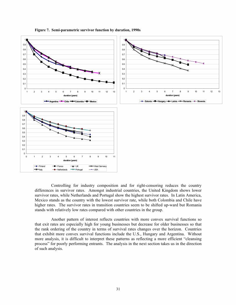
Figure 7. Semi-parametric survivor function by duration, 1990s

0

0.1

0.2

0.3

0.4

0.5

0.6

0.7

0.8

0.9

1

1 2 3 4 5 6 7 8 9 10 11 12 13

duration (years)

Argentina Chile Colombia Mexico

0

0.1

0.2

0.3

0.4

0.5

0.6

0.7

0.8

0.9

1

0 1 2 3 4 5 6 7 8 9 10 11

duration (years)

Finland France UK West GermanyItaly Netherlands Portugal USA

0

0.1

0.2

0.3

0.4

0.5

0.6

0.7

0.8

0.9

1

1 2 3 4 5 6 7 8 9 10 11 12 13

duration (years)

Estonia Hungary Latvia Romania Slovenia

Controlling for industry composition and for right-censoring reduces the countrydifferences in survivor rates. Amongst industrial countries, the United Kingdom shows lowersurvivor rates, while Netherlands and Portugal show the highest survivor rates. In Latin America,Mexico stands as the country with the lowest survivor rate, while both Colombia and Chile havehigher rates. The survivor rates in transition countries seem to be shifted up-ward but Romania stands with relatively low rates compared with other countries in the group.

Another pattern of interest reflects countries with more convex survival functions so that exit rates are especially high for young businesses but decrease for older businesses so thatthe rank ordering of the country in terms of survival rates changes over the horizon. Countriesthat exhibit more convex survival functions include the U.S., Hungary and Argentina. Withoutmore analysis, it is difficult to interpret these patterns as reflecting a more efficient “cleansingprocess” for poorly performing entrants. The analysis in the next section takes us in the directionof such analysis.

31

5. The effects of creative destruction on productivity

Reallocation and Productivity: Growth vs. Level Comparisons

In the previous two sections we have presented evidence of significant cross-countrydifferences in firm characteristics, their market dynamics and post-entry performance whichcannot be fully explained by differences in sectoral composition of the economy but rather pointsto salient differences in market characteristics and in business environment. The next obvious question is: do these differences matter for aggregate performance? We address this question in a number of ways. First, we examine the connection between productivity growth and the reallocation dynamics that we have documented in the prior sections. We are particularlyinterested in the contribution of entering and exiting businesses as well as the contribution of thereallocation of activity amongst continuing businesses. However, such analysis of the contribution of reallocation to productivity growth across countries, while inherently interesting,is fraught with interpretational difficulties given our discussion in section 2 and also potentiallyproblematic due to measurement difficulties given our discussion in section 3. We attempt to overcome some aspects of these difficulties by exploiting sectoral variation within countries inthis analysis and then in turn comparing such sectoral differences between countries (i.e., a difference-in-difference approach). In addition, we explore a cross sectional decomposition ofproductivity that turns out to be simpler and more robust in terms of theoretical predictions andmeasurement.

Reallocation and Productivity Growth

Using as building blocks productivity at the firm level, as well as the inputs used inproduction, productivity for each industry can be decomposed into the contribution of continuing firms, entrants and exiting firms21

Let’s define the sector-wide productivity level in year t, Pt as:

Pt iipt it [7]

where i is the employment share of firm i and Pt and pit are a productivity measure (in this analysis, labor productivity).

We have used three different methods for the decomposition of productivity growth. The first by Foster, Haltiwanger and Krizan (FHK henceforth, 2001)22 decomposes aggregateproductivity growth into five components, commonly called the ‘within effect’, ‘between effect’,‘cross effect’, ‘entry effect’, and ‘exit effect’, as follows:

21. Besides the industry decompositions of productivity, data also are collected on aggregateindustry productivity levels and growth rates, un-weighted average productivity of continuingfirms, entrants and exiters, and on the standard deviation of the distribution of productivity ofcontinuers, entrants and exiters.

22. Bartelsman and Doms (2000) also use this equation but date the exiters productivity in t; this isan unfortunate typographical error.

32

)()(

)(

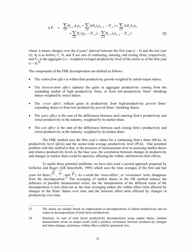
ktkitXi

kitktitNi

it

Ciititkt

Cikititit

Cikit

t

PpPp

pPppP [8]

where means changes over the k-years’ interval between the first year (t k) and the last year(t); it is as before; C, N, and X are sets of continuing, entering, and exiting firms, respectively;and Pt-k is the aggregate (i.e., weighted average) productivity level of the sector as of the first year(t k).23

The components of the FHK decomposition are defined as follows:

The within-firm effect is within-firm productivity growth weighted by initial output shares.

The between-firm effect captures the gains in aggregate productivity coming from the expanding market of high productivity firms, or from low-productivity firms’ shrinkingshares weighted by initial shares.

The ‘cross effect’ reflects gains in productivity from high-productivity growth firms’expanding shares or from low-productivity growth firms’ shrinking shares.

The entry effect is the sum of the differences between each entering firm’s productivity andinitial productivity in the industry, weighted by its market share.

The exit effect is the sum of the differences between each exiting firm’s productivity and initial productivity in the industry, weighted by its market share.

The FHK method uses the first year’s values for a continuing firm’s share ( it-k), its productivity level (pit-k) and the sector-wide average productivity level (Pt-k). One potentialproblem with this method is that, in the presence of measurement error in assessing market shares and relative productivity levels in the base year, the correlation between changes in productivityand changes in market share could be spurious, affecting the within- and between-firm effects.

To tackle these potential problems, we have also used a second approach proposed byGriliches and Regev (GR henceforth, 1995) which uses the time averages of the first and last

years for them ( i , ip , and P ). As a result the ‘cross-effect’, or ‘covariance’ term, disappearsfrom the decomposition.24 The averaging of market shares in the GR method reduces theinfluence of possible measurement errors, but the interpretation of the different terms of the decomposition is less clear-cut as the time averaging makes the within effect term affected by changes in the firms' shares over time and the between effect term affected by changes in productivity over time.

23. The shares are usually based on employment in decompositions of labour productivity and onoutput in decompositions of total factor productivity.

24. Similarly, in case of total factor productivity decomposition using output shares, randommeasurement errors in output could yield a positive covariance between productivity changesand share changes, and hence, within effect could be spuriously low.

33

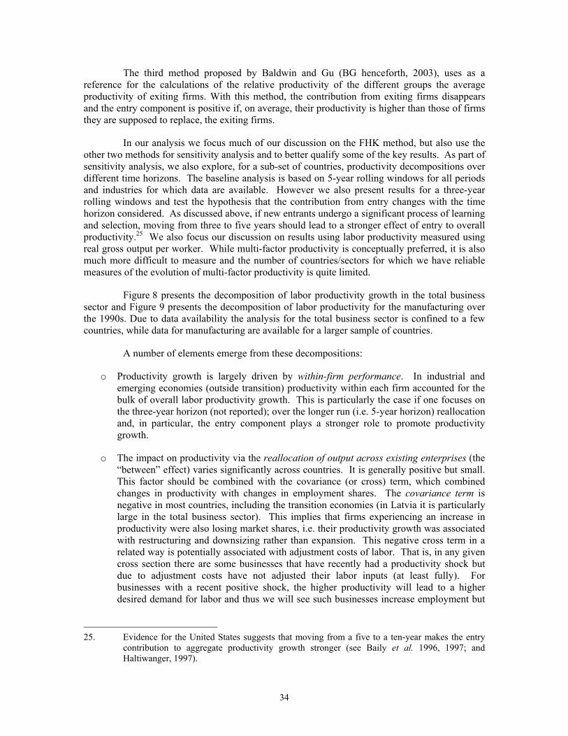
The third method proposed by Baldwin and Gu (BG henceforth, 2003), uses as areference for the calculations of the relative productivity of the different groups the average productivity of exiting firms. With this method, the contribution from exiting firms disappearsand the entry component is positive if, on average, their productivity is higher than those of firmsthey are supposed to replace, the exiting firms.

In our analysis we focus much of our discussion on the FHK method, but also use the other two methods for sensitivity analysis and to better qualify some of the key results. As part of sensitivity analysis, we also explore, for a sub-set of countries, productivity decompositions over different time horizons. The baseline analysis is based on 5-year rolling windows for all periodsand industries for which data are available. However we also present results for a three-yearrolling windows and test the hypothesis that the contribution from entry changes with the time horizon considered. As discussed above, if new entrants undergo a significant process of learningand selection, moving from three to five years should lead to a stronger effect of entry to overallproductivity.25 We also focus our discussion on results using labor productivity measured usingreal gross output per worker. While multi-factor productivity is conceptually preferred, it is alsomuch more difficult to measure and the number of countries/sectors for which we have reliable measures of the evolution of multi-factor productivity is quite limited.

Figure 8 presents the decomposition of labor productivity growth in the total businesssector and Figure 9 presents the decomposition of labor productivity for the manufacturing overthe 1990s. Due to data availability the analysis for the total business sector is confined to a few countries, while data for manufacturing are available for a larger sample of countries.

A number of elements emerge from these decompositions:

o Productivity growth is largely driven by within-firm performance. In industrial andemerging economies (outside transition) productivity within each firm accounted for the bulk of overall labor productivity growth. This is particularly the case if one focuses on the three-year horizon (not reported); over the longer run (i.e. 5-year horizon) reallocation and, in particular, the entry component plays a stronger role to promote productivitygrowth.

o The impact on productivity via the reallocation of output across existing enterprises (the “between” effect) varies significantly across countries. It is generally positive but small. This factor should be combined with the covariance (or cross) term, which combinedchanges in productivity with changes in employment shares. The covariance term is negative in most countries, including the transition economies (in Latvia it is particularly large in the total business sector). This implies that firms experiencing an increase in productivity were also losing market shares, i.e. their productivity growth was associatedwith restructuring and downsizing rather than expansion. This negative cross term in arelated way is potentially associated with adjustment costs of labor. That is, in any given cross section there are some businesses that have recently had a productivity shock but due to adjustment costs have not adjusted their labor inputs (at least fully). Forbusinesses with a recent positive shock, the higher productivity will lead to a higher desired demand for labor and thus we will see such businesses increase employment but

25. Evidence for the United States suggests that moving from a five to a ten-year makes the entrycontribution to aggregate productivity growth stronger (see Baily et al. 1996, 1997; andHaltiwanger, 1997).

34

due to diminishing returns (in the presence of any fixed factors at the micro level) a decrease in productivity.

o Finally, the net contribution to overall labor productivity growth of the entry and exit of firms (net entry) is generally positive in most countries, accounting for between 20 percent and 50 per cent of total productivity growth. While the exit effect is always positive, i.e. the least productive firms exit the market contributing to raise the productivityaverage of those that survive, the entry contribution tend to be negative in most OECD countries and in the non-transition emerging economies. In transition economies, in allbut one country (Hungary over the three-year horizon) the entry of new firms makes apositive and often strong contribution to productivity. For most countries, while the contribution of net entry is positive, it is less than proportionate relative to the share ofemployment accounted for by firm turnover.

An open question is whether the observed differences across countries are accounted forby differences in market institutions and policies or whether they reflect different circumstancesand/or problems of measurement. As discussed in section 2 and section 3, drawing suchinferences from cross country evidence is difficult given that the policy environment may impactin a variety of ways and given the measurement problems. Still, there are some patterns worthnoting. In the transition economies in particular, there is a very high rate of firm turnover as ashare of total employment and entry accounts for a large (but less than proportionate to the shareof turnover) share of productivity growth. The large contribution of entry partly reflects the large rate of firm turnover but it also reflects by construction a positive gap between entrants andincumbents productivity. In interpreting the latter finding, it is useful to put it in the context of the high pace of turnover. In general, it is difficult to interpret differences across countries in the magnitude of the gap between entering and exiting businesses. For example, it might reflectfundamentals driving market selection with new businesses adopting the latest business practices (or in transition economies, new businesses adopting market business practices relative toincumbents) or it might reflect a very high entry barrier so that only very productive newbusinesses enter. However, the latter explanation might suggest that firm turnover rates should be reduced which does not appear to be the case for the transition economies. Still, for the transition economies the contribution of net entry is far from proportionate suggesting that there is substantial churning of businesses via entry and exit that is not productivity enhancing in transition economies.

It is also interesting to note that the entry of new firms has variable effects on overall productivity growth in OECD countries. On the whole, data for European countries show that new firms typically make a positive contribution to overall productivity growth, although the effect is generally of small magnitude. By contrast, entries make a negative contribution in theUnited States for most industries and a stronger than average contribution tends to come from the exit of low productivity firms. Interpreting these findings without more information is difficult.The weak performance of entrants in the U.S. might reflect greater experimentation in the U.S.so that for each entering cohort of entrants there is more selection and potentially more learning by doing. Some evidence in favor of this interpretation is provided in Haltiwanger, Jarmin and Schank (2003), Foster, Haltiwanger and Krizan (2001, 2002) and Bartelsman and Scarpetta (2004). The former paper provides evidence of greater market experimentation in the U.S.relative to Germany. The latter shows that in the U.S. that as the horizon lengthens in the U.S.,the contribution of net entry rises disproportionately. Moreover, Foster et. al. show that theincreased contribution of net entry is due to both selection of the low productivity entrants anddue to learning by doing to successful entrants.

35

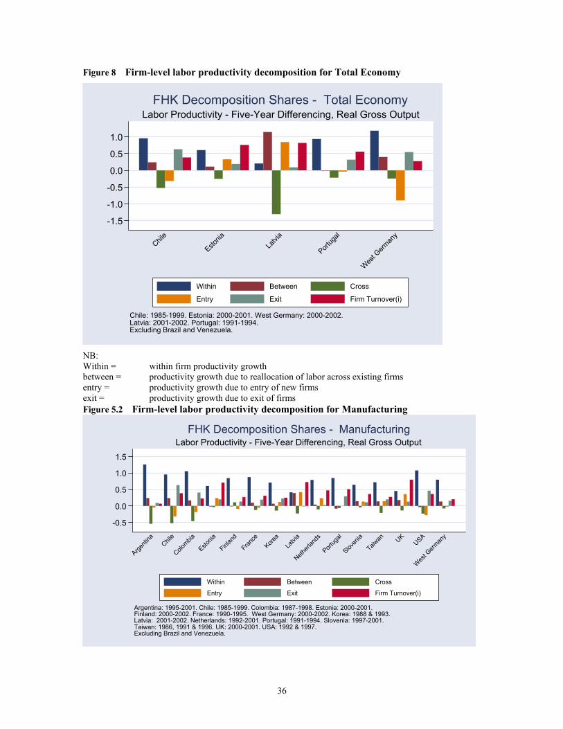
Figure 8 Firm-level labor productivity decomposition for Total Economy

-1.5

-1.0

-0.5

0.0

0.5

1.0

Chile

Estonia

Latvi

a

Portug

al

West G

erman

y

Chile: 1985-1999. Estonia: 2000-2001. West Germany: 2000-2002.Latvia: 2001-2002. Portugal: 1991-1994.Excluding Brazil and Venezuela.

Labor Productivity - Five-Year Differencing, Real Gross OutputFHK Decomposition Shares - Total Economy

Within Between Cross

Entry Exit Firm Turnover(i)

NB:Within = within firm productivity growthbetween = productivity growth due to reallocation of labor across existing firmsentry = productivity growth due to entry of new firmsexit = productivity growth due to exit of firmsFigure 5.2 Firm-level labor productivity decomposition for Manufacturing

-0.5

0.0

0.5

1.0

1.5

Argenti

naChil

e

Colombia

Estonia

Finlan

d

France

Korea

Latvi

a

Netherl

ands

Portug

al

Sloven

ia

Taiwan UK

USA

West G

erman

y

Argentina: 1995-2001. Chile: 1985-1999. Colombia: 1987-1998. Estonia: 2000-2001.Finland: 2000-2002. France: 1990-1995. West Germany: 2000-2002. Korea: 1988 & 1993.Latvia: 2001-2002. Netherlands: 1992-2001. Portugal: 1991-1994. Slovenia: 1997-2001.Taiwan: 1986, 1991 & 1996. UK: 2000-2001. USA: 1992 & 1997.Excluding Brazil and Venezuela.

Labor Productivity - Five-Year Differencing, Real Gross OutputFHK Decomposition Shares - Manufacturing

Within Between Cross

Entry Exit Firm Turnover(i)

36

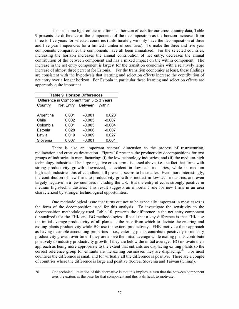
To shed some light on the role for such horizon effects for our cross country data, Table 9 presents the difference in the components of the decomposition as the horizon increases fromthree to five years for selected countries (unfortunately we only have the decomposition at threeand five year frequencies for a limited number of countries). To make the three and five yearcomponents comparable, the components have all been annualized. For the selected countries, increasing the horizon increases the annual contribution of net entry, decreases the annualcontribution of the between component and has a mixed impact on the within component. The increase in the net entry component is largest for the transition economies with a relatively large increase of almost three percent for Estonia. For the transition economies at least, these findings are consistent with the hypothesis that learning and selection effects increase the contribution of net entry over a longer horizon. For Estonia in particular these learning and selection effects areapparently quite important.

Table 9 Horizon Differences Difference in Component from 5 to 3 YearsCountry Net Entry Between Within

Argentina 0.001 -0.001 0.028Chile 0.002 -0.005 -0.007Colombia 0.001 -0.005 -0.004Estonia 0.028 -0.006 -0.007Latvia 0.019 -0.009 0.027Slovenia 0.007 -0.001 0.001

There is also an important sectoral dimension to the process of restructuring,reallocation and creative destruction. Figure 10 presents the productivity decompositions for twogroups of industries in manufacturing: (i) the low technology industries; and (ii) the medium-hightechnology industries. The large negative cross-term discussed above, i.e. the fact that firms withstrong productivity growth downsized, is evident in low-tech industries, while in mediumhigh-tech industries this effect, albeit still present, seems to be smaller. Even more interestingly,the contribution of new firms to productivity growth is modest in low-tech industries, and even largely negative in a few countries including the US. But the entry effect is strongly positive inmedium high-tech industries. This result suggests an important role for new firms in an areacharacterized by stronger technological opportunities.

One methodological issue that turns out not to be especially important in most cases is the form of the decomposition used for this analysis. To investigate the sensitivity to the decomposition methodology used, Table 10 presents the difference in the net entry component(annualized) for the FHK and BG methodologies. Recall that a key difference is that FHK usethe initial average productivity of all plants as the base from which to deviate the entering and exiting plants productivity while BG use the exiters productivity. FHK motivate their approach as having desirable accounting properties – i.e., entering plants contribute positively to industryproductivity growth over time if they are above the initial average while exiting plants contributepositively to industry productivity growth if they are below the initial average. BG motivate theirapproach as being more appropriate to the extent that entrants are displacing exiting plants so thecorrect reference group for entrants are the exiting businesses they are displacing.26 For mostcountries the difference is small and for virtually all the difference is positive. There are a coupleof countries where the difference is large and positive (Korea, Slovenia and Taiwan (China)).

26. One technical limitation of this alternative is that this implies in turn that the between componentuses the exiters as the base for that component and this is difficult to motivate.

37

Figure 10 Productivity decomposition by technology groups

-1.5-1.0-0.50.00.51.0

Argenti

naChil

e

Colombia

Estonia

Finlan

d

France

Korea

Latvi

a

Netherl

ands

Portug

al

Sloven

ia

Taiwan UK

USA

West G

erman

y

Argentina: 1995-2001. Chile: 1985-1999. Colombia: 1987-1998. Estonia: 2000-2001.Finland: 2000-2002. France: 1990-1995. West Germany: 2000-2002. Korea: 1988 & 1993.Latvia: 2001-2002. Netherlands: 1992-2001. Portugal: 1991-1994. Slovenia: 1997-2001.Taiwan: 1986, 1991 & 1996. UK: 2000-2001. USA: 1992 & 1997.Excluding Brazil and Venezuela.

Labor Productivity - Five-Year Differencing, Real Gross OutputFHK Decomposition Shares - Low Tech Industries

Within Between Cross

Entry Exit

-1.0

0.0

1.0

2.0

Argenti

naChil

e

Colombia

Estonia

Finlan

d

France

Korea

Latvi

a

Netherl

ands

Portug

al

Sloven

ia

Taiwan UK

USA

West G

erman

y

Argentina: 1995-2001. Chile: 1985-1999. Colombia: 1987-1998. Estonia: 2000-2001.Finland: 2000-2002. France: 1990-1995. West Germany: 2000-2002. Korea: 1988 & 1993.Latvia: 2001-2002. Netherlands: 1992-2001. Portugal: 1991-1994. Slovenia: 1997-2001.Taiwan: 1986, 1991 & 1996. UK: 2000-2001. USA: 1992 & 1997.Excluding Brazil and Venezuela.

Labor Productivity - Five-Year Differencing, Real Gross Output

FHK Decomposition SharesMedium Low, Medium High and High Tech Industries

Within Between Cross

Entry Exit

38

It is intuitive that the effects should in general be small because for both methods thenet entry term depends critically on the difference between average productivity of entering andexiting businesses. Put differently, both the entry and the exit term subtract off whatever base isused, so at first glance it might appear that the base is irrelevant (the base term in each componentcancels out in the net). Consistent with this perspective, computing the difference between theFHK and BG net entry terms yields:

))(( Xkt

Xi Niktitkit PPBGFHK [9]

where Pt-k is the average productivity of incumbents and PXt-k is the average productivity of

exiting businesses in the base year. Thus, if the share of activity (in this case employment)accounted for by entering and exiting businesses is the same then the difference is zero. As seen in section 4, for most countries the share of activity accounted for by entry is about the same as that for exit with the latter typically slightly larger since exiting businesses tend to be larger than entering businesses. Thus, this difference in weights does not matter for most countries. However, for Korea and to a lesser extent Portugal and Taiwan (China), the share of employmentaccounted for by exit is substantially less than the share of employment accounted for by entry --hence the sensitivity for these countries.

Table 10:FHK-BGDifference in NetentryCountry Net Entry Exit/ Entry Share Incumbent/Exit

Difference DifferenceProductivityDifference

Argentina 0.006 -0.012 0.098Chile -0.015 -0.022 0.432Colombia 0.005 0.008 0.627Estonia -0.008 -0.031 0.28Finland -0.003 -0.013 0.251France 0.004 0.034 0.107Korea, Rep. -0.06 -0.122 0.495Latvia 0.01 -0.001 -0.037Netherlands 0.003 0.028 0.025Portugal -0.016 -0.039 0.394Slovenia 0.014 0.059 0.252Taiwan(China) -0.019 -0.077 0.264UK 0.008 0.148 0.051USA 0.004 0.012 0.299WestGermany 0 0.001 0.274Notes: The reported figures are the time series averages. The first column is the product of the second and third column. However, since the reportedfigures are averages over time, the identity may appear not to hold (the product of the averages is not the same as the average of the product).

39

The cross-sectional efficiency of the allocation of activity

So far, the creative destruction process has been discussed mostly from the point of view of productivity growth. This is natural in this context since the creative destruction processis inherently dynamic. However, as discussed above and in section 2 at some length, distortionsin market structure and institutions can distort the entry and exit margins in a variety of waysmaking the interpretation of the dynamic decompositions discussed above difficult. Analternative simpler and more robust approach is to ask the question – are resources allocatedefficiently in a sector/country in the cross section at a given point in time. Dynamics can also be examined here to the extent that the nature of the efficiency of the cross sectional allocation of businesses can vary over time.

This approach is based upon a simple cross-sectional decomposition of productivitygrowth developed by Olley and Pakes (1996). They note that in the cross section, the level of productivity for a sector at a point in time can be decomposed as follows:

iti i

itittt PPNP )/1( [10]

where N is the number of businesses in the sector and is the operator that represents the crosssectional deviation of the firm-level measure from the industry simple average. The simpleinterpretation of this decomposition is that aggregate productivity can be decomposed into two terms involving the unweighted average of firm-level productivity plus a cross term that reflects the cross-sectional efficiency of the allocation of activity. The cross term captures allocative efficiency since it reflects the extent to which firms with greater efficiency have a greater marketshare.

This simple decomposition is very easy to implement and essentially involves justmeasuring the unweighted average productivity vs. the weighted average productivity.Measurement problems make comparisons of the levels of either of these measures across sectorsor countries very problematic but taking the difference between these two measures reflects a form of a difference-in-difference approach. Beyond measurement advantages, this approachalso has the related virtue that theoretical predictions are more straightforward as well.Distortions to market structure and institutions unambiguously imply that the difference betweenweighted and unweighted productivity (or equivalently the cross term) should be smaller.

With these remarks in mind, Figure 11 presents the measure of the gap betweenweighted and unweighted average productivity for a sample of countries. The Figure shows thedifference between the employment-weighted (logarithm of) labor productivity and theun-weighted average (logarithm of) labor productivity, and measures how many percent higheraggregate manufacturing labor productivity is than average labor productivity of firms inmanufacturing. The EU countries enjoy a 25 percent productivity boost from rational allocation of resources, but have not seen much change on balance over time. SE Asian economies are on top, followed by the U.S., while the Latin American countries, except Argentina, show higherproductivity boosts through resource allocation than the EU, but lower than in SE Asia.

40

Figure 11 The gap between weighted and un-weighted labor productivity, 1990s

0.0

0.2

0.4

0.6

0.8

Argenti

naChil

e

Colombia

UK old

Finlan

d

Netherl

ands

France

West G

erman

y

Portug

alUSA

Taiwan

Korea

Indon

esia

Sloven

iaLa

tvia

Roman

ia

Hunga

ry

Estonia

Data for Hungary, Indonesia and Romania use Three-Year Differencing.Excluding Brazil and Venezuela.

Five-Year Differencing, Real Gross Output, Manufacturing

The Gap Between Weighted and Un-WeightedLabor Productivity, 1990s

Figure 12 presents the evolution over the 1990s in the transition economies. As may beseen, the transition economies all start out at very low and sometimes negative allocation effects.A negative effect means that allocation was worse than that resulting from a toss of the dice: for some reason resources were disproportionately allocated towards poor productivity firms.However, the transition countries generally exhibit a rapid increase of this ratio over timeconsistent with the view that allocative efficiency improved substantially in the transition economies over this time period.

Figure 12 The evolution of the gap between weighted and un-weighted productivity in transition economies over the 1990s

0.0

0.2

0.4

0.6

0.8

Estonia

, 199

5

Estonia

, 200

1

Hunga

ry, 19

92

Hunga

ry, 19

95

Hunga

ry, 20

01

Latvi

a, 19

96

Latvi

a, 20

01

Roman

ia,19

95

Roman

ia, 19

99

Sloven

ia, 19

92

Sloven

ia, 19

95

Sloven

ia, 20

01

Five-Year Differencing, Real Gross Output, Manufacturing.Data for Hungary and Romania use Three-Year Differencing.

in Transition Economies over the 1990s

The Evolution of the Gap Between Weightedand Un-Weighted Labor Productivity

41

Contestability Effects: The Relationship Between the Pace of Creative Destruction andProductivity Growth

The analysis above focuses on the direct contribution of the reallocation process forproductivity growth (either with the dynamic or cross sectional decomposition). These decompositions lead one to think about the reallocation contributions and the within firmcontributions as being alternative explanations of productivity growth. The reallocation contributions are often interpreted in the literature as reflecting the creative destruction processes while the within firm are interpreted as reflecting more traditional sources of productivity growth(the average firm becomes more productive with advancing technology. However, rather thanbeing alternatives, these effects (within vs. reallocation) may be closely related. That is, the paceof the creative destruction process might be interpreted as a measure of the contestability or competitive of markets. As such, greater competitive pressures may induce incumbents to perform more efficiently.

A first look at such contestability effects is provided in Figure 13. In this figure, we exploit notonly the cross country variation but the variation across industries in order to be able to increase the number of observations (and since in principle the above arguments should apply across sectors as well as countries). In particular, we examine the relationship between the contribution of net entry in a country/sector (using time averages from the country/sector/year data) and the productivity growth from incumbents (the within term in the FHK decomposition). Interestingly,we find a strong positive and statistically significant correlation between the net entrycontribution and the productivity growth of incumbents.

This finding is suggestive that there is a relationship between the creative destructive and within firm sources of productivity growth. If nothing else, this strong correlation suggests that thesecomponents are not orthogonal alternatives but rather closely related. It might be, however, thatthe correlation in Figure 13 is readily explained as reflecting the impact of technological advancesfor both continuing firms and for the creative destruction process. That is, it may be that withtechnological advances we observe incumbents who survive increase productivity and also observe entering businesses (who presumably adopt the latest advances) more productive that theexiting businesses.

To focus more on the contestability hypothesis directly, in Figure 14 we examine the relationshipbetween the firm turnover rate and the productivity growth of incumbents. We again find apositive and statistically significant correlation. This latter finding provides more direct evidence of a connection between the competitiveness or contestability of markets and the productivitygrowth within incumbent firms.

A related question is whether the pace of creative destruction is also related to the productivitydifference between entering and exiting businesses. Figure 15 shows the relationship between the firm turnover rate and the mean difference (unweighted) between the productivity of entering and exiting businesses. We find a strong and positive relationship here as well.27

27. Given the discussion in section 2, it is possible to justify either a positive or negative correlation.On the one hand, a higher firm turnover rate might imply greater dynamism and thus competitiveforces playing a greater role in determining market selection. From this perspective, thecorrelation should be positive and since we found this in the data this is the interpretation we are pushing. Alternatively, greater dynamism might also be due to greater randomness in marketselection and/or greater market experimentation (which adds a form of endogenous randomness).Such greater randomness in market selection would imply a negative correlation.

42

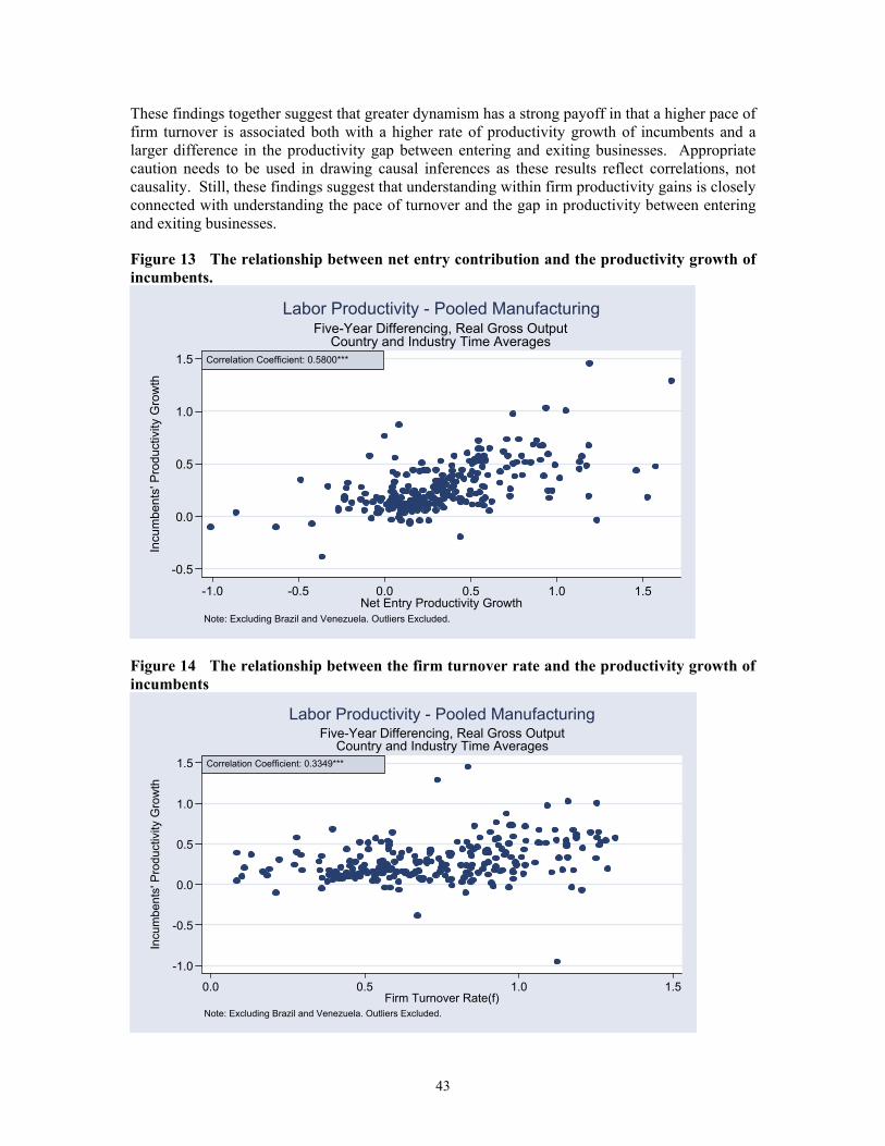
These findings together suggest that greater dynamism has a strong payoff in that a higher pace of firm turnover is associated both with a higher rate of productivity growth of incumbents and a larger difference in the productivity gap between entering and exiting businesses. Appropriate caution needs to be used in drawing causal inferences as these results reflect correlations, not causality. Still, these findings suggest that understanding within firm productivity gains is closelyconnected with understanding the pace of turnover and the gap in productivity between enteringand exiting businesses.

Figure 13 The relationship between net entry contribution and the productivity growth of incumbents.

-0.5

0.0

0.5

1.0

1.5

Incu

mbe

nts'

Pro

duct

ivity

Gro

wth

-1.0 -0.5 0.0 0.5 1.0 1.5Net Entry Productivity Growth

Note: Excluding Brazil and Venezuela. Outliers Excluded.

Correlation Coefficient: 0.5800***

Five-Year Differencing, Real Gross OutputCountry and Industry Time Averages

Labor Productivity - Pooled Manufacturing

Figure 14 The relationship between the firm turnover rate and the productivity growth ofincumbents

-1.0

-0.5

0.0

0.5

1.0

1.5

Incu

mbe

nts'

Pro

duct

ivity

Gro

wth

0.0 0.5 1.0 1.5Firm Turnover Rate(f)

Note: Excluding Brazil and Venezuela. Outliers Excluded.

Correlation Coefficient: 0.3349***

Five-Year Differencing, Real Gross OutputCountry and Industry Time Averages

Labor Productivity - Pooled Manufacturing

43

Figure 15 The relationship between the firm turnover rate and the mean productivity difference between entering and exiting businesses

0.0

0.5

1.0

1.5

Mea

n D

iffer

ence

in E

ntry

and

Exi

t Pod

uctiv

ity

-1.0 -0.5 0.0 0.5 1.0 1.5Firm Turnover Rate (f)

Note: Excluding Brazil and Venezuela. Outliers Excluded.

Correlation Coefficient: 0.2780***

Five-Year Differencing, Real Gross OutputCountry and Industry Time Averages

Labor Productivity - Pooled Manufacturing

6. Concluding remarks

In this paper we provide an in-depth analysis of the process of creative destructionacross 24 countries and 2-digit industries over the past decade. We rely on a newly assembled dataset that draws from different micro data sources (business registers, census, or representativeenterprise surveys). The novelty of our approach is in the harmonisation of firm level data acrosscountries, which enables international comparisons and the identification of country-specificfactors as opposed to sectoral and time effects. Our main goal is to assess how certain stylisedfacts presented in the micro-economic literature of creative destruction -- largely relying on U.S.data -- are confirmed by evidence from a range of countries, characterised by different economicstructures, institutions and aggregate growth performances over the period analysed.

Overall, our data clearly suggest a significant heterogeneity of firms in each market and country.This heterogeneity is manifested in large disparities in firm size, firm growth and productivityperformance. More in detail, we found:

The average size of incumbent firms varies widely across sectors and countries. Differences in firm size are largely driven by within-sector differences, although in some countries sectoral specialization also plays a significant role. Smaller countries tend to have a size distribution skewed towards smaller firms, but the average size of firms aswell as the dispersion within and across countries do not map precisely with the overall dimension of the domestic market.

Firm churning is large: gross firm turnover involves 10-20 percent of all firms in industrial countries, and even more in transition and other emerging economies.Entering, but also exiting, firms tend to be small and thus firm flows affect only about5-10 per cent of total employment. This suggests that the entry of small firms is

44

relatively easy, while larger-scale entry is more difficult but, survival among small firmsis also more difficult and many small new comers fails before reaching the efficient scaleof production.

Entry and exit rates are part of the same process. In most countries, entry and exit rates are correlated across industries. They are part of a process in which a large number of new firms displace a large number of obsolete firms (which may themselves be relativelynew), without affecting significantly the total number of firms in the market at each pointin time. Transition economies and some emerging countries show weaker correlationsbecause of stronger structural changes in their economy with declining traditional sectorsand expanding modern sectors.

Market selection is pretty harsh: about 20 to 40 per cent of entering firms fail within the first two years of life. Confirming previous results, failure rates decline with duration: conditional on surviving the first few years, the probability of survival becomes higher.But only about 40-50 per cent of total entering firms in a given cohort survive beyond the seventh year.

Successful entrants expand rapidly. Surviving firms are not only relatively larger but alsotend to grow rapidly. The combined effect of exits being concentrated amongst thesmallest units and the growth of survivors makes the average size of a given cohort to increase rapidly towards the efficient scale.

Creative destruction is important for promoting productivity growth. While the continuous process of restructuring and upgrading by incumbents is essential to boost aggregate productivity, the entry of new firms and the exit of obsolete units also play animportant role. The contribution of firm churning to productivity is particularlyimportant in high-tech industries -- where new technologies are often better harnessed by new firms.

Creative destruction also promotes market contestability. A strong process of creative destruction also promotes productivity-enhancing strategies of incumbents. We have some preliminary evidence of this “contestability” effect: there is a significant correlationbetween firm turnover rates and incumbent productivity growth across industries and countries; and there is also a significant correlation between the net entry contribution to productivity and incumbent productivity growth. In other words, higher firm turnover is associated with stronger productivity growth of incumbents, and the more effective the process of creative destruction is for productivity, the more it stimulates growth by incumbents.

Our analysis also shows significant differences across countries along the different dimensions ofour data: size, firm turnover, survival and productivity growth. These differences can be linkedtogether to form a tentative interpretation of the nature and effectiveness of creative destruction in different contexts.

Industrial countries. All industrial countries show a marked process of creative destruction. There are, however, some distinguishing features. There is a greater heterogeneity of firms in the US compared with European countries, and this heterogeneity is also reflected in the composition of entrant firms. New firms tend to be smaller in relative size than incumbents and with lower productivity levels than their counterparts in Europe. But market selection and learning effects imply that successful

45

surviving entrants expand rapidly generating stronger post-entry growth, while low productivity entrants exit rapidly freeing resources for new ventures. These features mayindicate a different degree of market experimentation in the United States compared withEurope. Related to this, the European countries exhibit markedly worse static allocationof resources than the U.S.

Transition economies. Creative destruction assumes an even stronger role in the five Central and Eastern European countries in transition. The magnitude of firm creation and destruction is generally larger than that observed in industrial countries: many new smaller firms have been replacing obsolete larger units inherited from the central plan period. Moreover, new firms have filled in new market niches enjoying, especially in theearly years of transition, less competition and higher survival rates. But market forces have quickly strengthened, with some stabilization and equilibration in entry and exitrates, as well as with increasing failure rates among new firms. The process of resource reallocation has become increasingly effective over the transition, shifting resources tonew but also more productive firms. There are also interesting differences across countries. Hungary as well as some small open economies in transition (Estonia, Latvia and Slovenia) have all experienced a strong creative destruction process, with large postentry growth and a marked contribution of the new entry (as well as exit) to productivitygrowth. Romania is still dominated by some large firms; entry of new firms haveincreased rapidly in recent years when market reforms were advanced, but even successful new firms seem to have difficulty in expanding.

Emerging economies of Latin America and East Asia. It is more difficult to trace common patterns for the other emerging economies. Mexico shows strong market dynamism, with large entry and exit flows, strong market selection of new entrants and strong post entry growth of successful entrants. NAFTA likely created an environmentthat was conducive to such growth. By contrast, Argentina resembles more somecontinental European countries with somewhat lower firm turnover, yet strong marketselection that however is not associated with large post entry growth of successful firms.Moreover, creative destruction seems to play a relatively small role in promotingproductivity growth. For the other Latin American countries, data cover onlymanufacturing and firms above a certain size, making comparisons more difficult.Finally, Korea, Indonesia and Taiwan (China) all show that creative destruction plays a strong role in promoting productivity growth.

46

References

Ahn, S. (2000). “Firm dynamics and Productivity Growth: A Review of Micro Evidence fromOECD Countries.” OECD Economics Department Working Paper No. 297, Paris.

Aw, B.Y., S. Chung and M. Roberts (2002). “Productivity, Output, and Failure: A Comparison of Taiwanese and Korean Manufacturers.” NBER Working Paper 8766, forthcoming in Economic Journal.

Baily, Martin N., Charles Hulten, and David Campbell (1992). “Productivity Dynamics in Manufacturing Establishments.” Brookings Papers on Economic Activity: Microeconomics,pp. 187-249.

Baldwin, J. and W. Gu (2003). “Plant turnover and productivity growth in Canadian manufacturing.” Statistics Canada, April.

Baldwin, J.R. and P.K. Gorecki (1991). “Entry, Exit, and Productivity Growth”, in: P.A. Geroski and J. Schwalbach, eds. Entry and Market Contestability: An International Comparison,Blackwell, Oxford.

Bartelsman Eric J. (2004). “The analysis of microdata from an international perspective.” OECD Statistics Directorate, STD/CSTAT, 12.

Bartelsman, Eric and Stefano Scarpetta (2004). "Experimentation within and between firms: Anyrole for policy and institutions?.” Paper presented at the 2004 American Economic Association Meeting, San Diego, January 3-5.

Bartelsman, Eric J. and Mark Doms (2000). “Understanding Productivity: Lessons fromLongitudinal Microdata.” Journal of Economic Literature 38(3), pp. 569-95.

Bartelsman, Eric J., Stefano Scarpetta and John Halitwanger (2004). “Distributed Analysis ofFirm-level data from Industrial and Developing Countries.” mimeo.

Bastos, F. and J. Nasir (2004). “Productivity and the Investment Climate: What Matters Most?.” Working Paper.

Brown, David J. and John S. Earle (2004). “Economic Reforms and Productivity-EnhancingReallocation in Post-Soviet Transtion.” Upjohn Institute Staff Working Paper No. 04-98.

Caballero R.J. and M.L. Hammour (1994). “The Cleansing Effect of Creative Destruction.” American Economic Review 84:5, pp. 1350-68.

Caballero R.J. and M.L. Hammour (2000). “Creative Destruction and Development: Institutions, Crises, and Restructuring.” National Bureau of Economic Research, Inc, NBER Working Papers: 7849.

Cabral, Luis (1995). “Sunk Costs, Firm Size and Firm Growth.” Journal of Industrial Economics43:2 (June), pp. 161-72.

Cabral,-Luis-M-B; Mata,-Jose (2003). “On the Evolution of the Firm Size Distribution: Facts and Theory.” American-Economic-Review 93:4 (September), pp. 1075-90.

Campbell, J. (1998). “Entry, Exit, Embodied Technology, and Business Cycles.” Review of Economic Dynamics 1:2 (April), pp. 371-408.

Caves, R.E. (1998). “Industrial Organization and New Findings on the Turnover and Mobility ofFirms.” Journal of Economic Literature 36:4, pp. 1947-82.

47

Cooper, R., J. Haltiwanger and L. Power (1997). “Machine replacement and the business cycle:lumps and bumps.” NBER Working Paper No. 5260 (revised).

Davis, Steven and John Haltiwanger (1999). “Gross Job Flows.” in David Card and Orley Ashenfelter eds. the Handbook of Labor Economics, North-Holland.

Davis, Steven, John Haltiwanger and Scott Schuh (1996). Job Creation and Destruction, MIT Press.

Davis, S.J. and Henrekson, M. (1999). “Explaining National Differences in the Size and IndustryDistribution of Employment.” Small Business Economics 12, pp. 59-83.

Dollar, D., M. Hallward-Driemeier, and T. Mengistae (2003). “Investment Climate and FirmPerformance in Developing Economies.” World Bank, Development Research Group,Washington, D.C.

Dunne, T., M. Roberts and L. Samuelson (1989). “The Growth and Failure of U.S. Manufacturing Plants.” Quarterly Journal of Economics 104, pp. 671-98.

Dunne, T., M. Roberts and L. Samuelson (1988). “Patterns of Firm Entry and Exit in US Manufacturing Industries.” Rand Journal of Economics 19:4, pp. 495-515.

Elmeskov, Jorgen, Martin, John P. and Scarpetta, Stefano (1998). “Key Lessons for Labour Market Reforms: Evidence from OECD Countries' Experiences.” Swedish EconomicPolicy Review Autumn 5, iss. 2, pp. 205-52.

Ericson, Richard and Ariel Pakes (1995). “Markov-Perfect Industry Dynamics: A Framework for Empirical Work.” Review of Economic Studies 62:1, pp. 53-82.

Eslava, Marcela, John Haltiwanger, Adriana Kugler, and Maurice Kugler (2004). “The Effects ofStructural Reforms on Productivity and Profitability Enhancing Reallocation.” Journal of Development Economics (forthcoming).

Evans, David (1987a). “The relationship between firm growth, size and age: Estimates for 100manufacturing industries.” Journal of Industrial Economics 35:4 (June), pp. 567-581.

Evans, David (1987b). “Tests for alternative theories of firm growth.” Journal of PoliticalEconomy 95:4 August, pp. 657-674.

Foster, Lucia, Haltiwanger, John, and C.J. Krizan (2001). “Aggregate Productivity Growth: Lessons from Microeconomic Evidence.” in Edward Dean, Michael Harper and Charles Hulten eds. New Developments in Productivity Analysis, Chicago: University of ChicagoPress.

Foster, Lucia, John Haltiwanger, and C.J. Krizan (2002). “The Link Between Aggregate and Micro Productivity Growth: Evidence from Retail Trade.” NBER Working Paper.

Geroski, Paul (1991). “Market dynamics and entry”, Oxford: Basil Blackwell.

Geroski, Paul (1995). “What do we Know about Entry?” International Journal Of Industrial Organization 13, pp. 421-440.

Griliches,-Zvi; Regev,-Haim (1995). “Firm Productivity in Israeli Industry: 1979-1988.” Journalof Econometrics 65:1 (January), pp.175-203.

Hallward-Driemeier, Mary, Scott Wallsten, Lixin Collin Xu (2004). “The Investment Climate and the Firm: Firm-Level Evidence from China.” mimeo.

48

49

Haltiwanger, John, Ron Jarmin, and Thorsten Schank, (2003) “Productivity, Investment in ICT and Market Experimentation: Micro Evidence from Germany and the U.S., Center for Economic Studies Working Paper.

Haltiwanger, J. and H. Schweiger (2004). “Firm Performance and the Business Climate: Where Does ICA Fit In?” Working Paper.

Helpman, E. M. Melitz, and S. Yeaple, (2004). “Export versus FDI with Heterogeneous Firms.”American Economic Review 94 (March), n1, pp. 300-316.

Hopenhayn, Hugo A. (1992). “Entry, Exit, and Firm Dynamics in Long Run Equilibrium.” Econometrica 60:5, pp. 1127-50.

Jovanovic, Boyan (1982). “Selection and the Evolution of Industry.” Econometrica 50:3, pp. 649-70.

Jovanovic, Boyan and Glenn MacDonald (1994). “The life cycle of a competitive industry.” Journal of Political Economy 102:2, pp. 322-347.

Klepper, Steven (1996). “Entry, exit, growth, and innovation over the product cycle”, American Economic Review 86:3 (June), pp. 562-83.

Klepper Steven and Elizabeth Graddy (1990). “The evolution of new industries and the determinants of of market structure.” Rand J. of Economics 21:1 (Spring), pp. 27-44.

Klepper Steven and Kenneth Simons (1993). “Technological Change and Industry Shakehouts.” Working Paper, Carnegie Mellon, U. Pittsburgh.

Klette, Tor Jakob and Zvi Griliches (1996). “The Inconsistency of Common Scale Estimators When Output Prices Are Unobserved and Endogenous.” Journal of Applied Econometrics11:4, pp. 343-61.

Levinsohn, J. and A.Petrin (1999). “When Industries Become More Productive, Do Firms? Investigating Productivity Dynamics.” NBER Working Paper 6893.

Mortensen, D. and C. Pissarides (1994). “Job creation and destruction in the theory of unemployment.” Review of Economic Studies 61, pp. 397-416.

Olley, G. Steven and Ariel Pakes (1996). "The Dynamics of Productivity in the Telecommunications Equipment Industry." Econometrica, 64:6, pp. 1263-97.

Pakes, Ariel and Richard Ericson (1998). “Empirical Implications of Alternative Models of Firm Dynamics.” J. Econ. Theory 79:1, pp. 1-45.

Roberts, M. and J. Tybout (1997). “ Producer Turnover and Productivity Growth in Developing Countries” (with James Tybout), The World Bank Research Observer (February).

Sutton, John (1997). “Gibrat’s Legacy.” Journal of Economic Literature 35:1, pp. 40-59.