creative computing ii: interactive multimedia volume...
TRANSCRIPT
Creative computing II: interactive
multimedia
Volume 1: Creative signals and systems
M. Casey with S. Rauchas
2910227
2008
Undergraduate study in
Computing and Related Subjects
The material in this subject guide was prepared for the University of LondonExternal System by:
Michael Casey, Goldsmiths Digital Studios, Goldsmiths, University of LondonSarah Rauchas, Department of Computing, Goldsmiths, University of London.
The guide was produced by Sarah Rauchas, Department of Computing, Goldsmiths,
University of London. Many thanks to Jonathan Barbara, SMIIT, Malta, for
identifying typographical and code inconsistencies.
This is one of a series of subject guides published by the University.
This subject guide is for the use of University of London External System students
registered for programmes in the field of Computing. The programmes currently
available in these subject areas are:
BSc(Honours) in Computing and Information Systems
BSc(Honours) in Creative ComputingDiploma in Computing and Information Systems
Diploma in Creative Computing
Published 2008
Copyright c© University of London Press 2008
Publisher:The External System
Publications OfficeUniversity of London
Stewart House
32 Russell SquareLondon
WC1B 5DN
www.londonexternal.ac.uk
All rights reserved. No part of this work may be reproduced in any form, or by anymeans, without permission in writing from the publisher. This material is not
licensed for resale.

Contents
Preface iii
1 Perception 11.1 Introduction . . . . . . . . . . . . . . . . . . . . . . . . . . . . . . . . . 1
1.2 Cognitive and psychological aspects of perception . . . . . . . . . . . . 11.3 Abstraction in perception . . . . . . . . . . . . . . . . . . . . . . . . . 2
1.4 Ambiguity in perception . . . . . . . . . . . . . . . . . . . . . . . . . . 3
1.5 Summary and learning outcomes . . . . . . . . . . . . . . . . . . . . . 51.6 Exercises . . . . . . . . . . . . . . . . . . . . . . . . . . . . . . . . . . . 5
2 Creative signals 72.1 Introduction . . . . . . . . . . . . . . . . . . . . . . . . . . . . . . . . . 72.2 Waves . . . . . . . . . . . . . . . . . . . . . . . . . . . . . . . . . . . . 7
2.3 Signal processing . . . . . . . . . . . . . . . . . . . . . . . . . . . . . . 82.3.1 RADAR . . . . . . . . . . . . . . . . . . . . . . . . . . . . . . . 9
2.3.2 Audio signals . . . . . . . . . . . . . . . . . . . . . . . . . . . . 9
2.3.3 Image signals . . . . . . . . . . . . . . . . . . . . . . . . . . . . 102.3.4 Visual art and music . . . . . . . . . . . . . . . . . . . . . . . . 10
2.4 Signal definition . . . . . . . . . . . . . . . . . . . . . . . . . . . . . . 11
2.4.1 Independent variables in signals and systems . . . . . . . . . . 122.5 Summary and learning outcomes . . . . . . . . . . . . . . . . . . . . . 13
2.6 Exercises . . . . . . . . . . . . . . . . . . . . . . . . . . . . . . . . . . . 13
3 Signals 153.1 Introduction . . . . . . . . . . . . . . . . . . . . . . . . . . . . . . . . . 15
3.2 Octave . . . . . . . . . . . . . . . . . . . . . . . . . . . . . . . . . . . . 153.2.1 Installing Octave . . . . . . . . . . . . . . . . . . . . . . . . . . 16
3.2.2 Installing for different operating systems . . . . . . . . . . . . . 16
3.2.3 Running Octave . . . . . . . . . . . . . . . . . . . . . . . . . . . 163.2.4 Using Octave . . . . . . . . . . . . . . . . . . . . . . . . . . . . 17
3.3 What are signals? . . . . . . . . . . . . . . . . . . . . . . . . . . . . . . 293.3.1 One-dimensional signals . . . . . . . . . . . . . . . . . . . . . . 29
3.3.2 Octave representation of discrete-time signals . . . . . . . . . . 31
3.3.3 The unit impulse . . . . . . . . . . . . . . . . . . . . . . . . . . 363.3.4 The unit step . . . . . . . . . . . . . . . . . . . . . . . . . . . . 37
3.3.5 The unit delay . . . . . . . . . . . . . . . . . . . . . . . . . . . 38
3.3.6 Delay operations in Octave . . . . . . . . . . . . . . . . . . . . 413.4 Audio signals . . . . . . . . . . . . . . . . . . . . . . . . . . . . . . . . 42
3.4.1 Sampling . . . . . . . . . . . . . . . . . . . . . . . . . . . . . . 423.4.2 Frequency . . . . . . . . . . . . . . . . . . . . . . . . . . . . . . 43
3.4.3 Amplitude . . . . . . . . . . . . . . . . . . . . . . . . . . . . . . 47
3.4.4 Phase . . . . . . . . . . . . . . . . . . . . . . . . . . . . . . . . 493.5 Summary and learning outcomes . . . . . . . . . . . . . . . . . . . . . 55
3.6 Exercises . . . . . . . . . . . . . . . . . . . . . . . . . . . . . . . . . . . 55
4 Systems 594.1 Introduction . . . . . . . . . . . . . . . . . . . . . . . . . . . . . . . . . 59
4.2 LTI systems . . . . . . . . . . . . . . . . . . . . . . . . . . . . . . . . . 60
i

Creative computing II: interactive multimedia – Volume 1: Creative signals and systems
4.2.1 Linearity . . . . . . . . . . . . . . . . . . . . . . . . . . . . . . . 604.2.2 Time invariance . . . . . . . . . . . . . . . . . . . . . . . . . . . 61
4.2.3 Impulse response . . . . . . . . . . . . . . . . . . . . . . . . . . 614.2.4 Convolution . . . . . . . . . . . . . . . . . . . . . . . . . . . . . 62
4.2.5 Unit impulse and unit delay systems . . . . . . . . . . . . . . . 64
4.2.6 Scaled delay . . . . . . . . . . . . . . . . . . . . . . . . . . . . 654.2.7 Convolution revisited . . . . . . . . . . . . . . . . . . . . . . . 65
4.3 Spectral analysis . . . . . . . . . . . . . . . . . . . . . . . . . . . . . . 67
4.3.1 Complex exponentials . . . . . . . . . . . . . . . . . . . . . . . 674.3.2 Signal multiplication by complex exponentials . . . . . . . . . . 71
4.3.3 Spectra of signals and systems . . . . . . . . . . . . . . . . . . . 724.3.4 Fast Fourier Transform (FFT) . . . . . . . . . . . . . . . . . . . 73
4.3.5 Convolution by spectrum multiplication . . . . . . . . . . . . . 81
4.4 Summary and learning outcomes . . . . . . . . . . . . . . . . . . . . . 824.5 Exercises . . . . . . . . . . . . . . . . . . . . . . . . . . . . . . . . . . . 83
5 Audio and image filtering 855.1 Audio effects . . . . . . . . . . . . . . . . . . . . . . . . . . . . . . . . 85
5.1.1 EQ . . . . . . . . . . . . . . . . . . . . . . . . . . . . . . . . . . 85
5.1.2 FIR filter design . . . . . . . . . . . . . . . . . . . . . . . . . . . 885.1.3 Sweepable EQ . . . . . . . . . . . . . . . . . . . . . . . . . . . 90
5.1.4 Subtractive synthesis . . . . . . . . . . . . . . . . . . . . . . . . 92
5.1.5 Echo . . . . . . . . . . . . . . . . . . . . . . . . . . . . . . . . . 935.1.6 Reverberation . . . . . . . . . . . . . . . . . . . . . . . . . . . . 95
5.1.7 Resampling . . . . . . . . . . . . . . . . . . . . . . . . . . . . . 96
5.2 Image filtering . . . . . . . . . . . . . . . . . . . . . . . . . . . . . . . 995.2.1 Matrices . . . . . . . . . . . . . . . . . . . . . . . . . . . . . . . 99
5.2.2 Image representation . . . . . . . . . . . . . . . . . . . . . . . . 1055.2.3 Image effects . . . . . . . . . . . . . . . . . . . . . . . . . . . . 112
5.3 Summary and learning outcomes . . . . . . . . . . . . . . . . . . . . . 123
5.4 Exercises . . . . . . . . . . . . . . . . . . . . . . . . . . . . . . . . . . . 124
ii

Preface
This subject unit builds and extends on the work you did in Level 1, in developing
and expressing creative ideas using computers. The focus of the subject this year ison the combination of two things: signals and signal processing; and perception.
The approach taken in this guide is that sound and image, and other kinds ofcreative outputs, are at their very basis, signals: signals from light, signals from
vibration, that our senses receive and process. Perception therefore involves
examining how our senses process these signals; how the eyes process light, how theears process sound. There is also some discussion of how these processes are
experienced on a higher level, which is cognitive. The subject also includes a basic
look at animation. We can see this, very broadly, as looking at how human beingsprocess information (i.e. signals). To complete the unit, there is material covering
the processing of data of various kinds using computers.
At the end of this unit you will understand the basics of signal processing, and how
perception works, and be able to use this to create innovative artworks.
The subject guide for Creative Computing 2 is divided into two volumes. The first
volume, which is this one, focuses on signal processing. The second volume containsmaterial on perception, the processing of digital information and animation. It is
therefore very important that you become familiar with the contents of both this
volume and the second volume of the subject guide.
By the end of this unit, you should be able to implement creative concepts that are
not easily realised using commercial software packages and, therefore, you will beenabled to demonstrate a high degree of originality in your own creative work.
The assessment for this unit comprises four pieces of coursework and an unseenwritten examination. The examination questions will be about the background,
techniques and examples (including the figures presented) in Volume 1 and Volume2 of this subject guide, and the essential reading (see below). While not required,
you should read the items on the recommended reading list where possible to
increase your understanding of the general subject area, and sometimes for analternative explanation of important concepts, which you might find helpful. The
items on the additional reading list provide supplementary material that you might
find interesting and relevant. There is an accompanying study booklet on portfoliocreation, which is not examinable. However, developing a portfolio of work will be
an invaluable complement to your degree.
This subject guide is not a complete unit text on its own. It introduces topics and
concepts, and provides some material to help you to study the topics in the unit.Further reading is very important as you are expected to see an area of study from
an holistic point of view, and not just as a set of limited topics. Doing further reading
will also help you to understand complex concepts more completely.
iii
Creative computing II: interactive multimedia – Volume 1: Creative signals and systems
Essential reading
Eaton, J.W. GNU Octave Manual. (Bristol: Network Theory, 1996) [ISBN 0954161726].
(This is also available online in HTML form at
http://www.gnu.org/software/octave/doc/interpreter
and in texinfo source format in the Octave source code distribution.)
Recommended reading
Foley, J.D., A. van Dam and others Introduction to Computer Graphics. (Reading, Mass.; Wokingham: Addison Wesley,
1997) [ISBN 0201609215].
Howard, D.M. and J. Angus Acoustics and Psychoacoustics. (Oxford: Focal, 2006) [ISBN 0240519957 (pbk);
9780240519951].
Oppenheim, A.V. and A.S. Willsky with S. Hamid Nawab Signals and Systems. (Upper Saddle River, N.J.; London:
Prentice Hall, 1997) [ISBN 0138147574].
Reas, C. and B. Fry Processing: A Programming Handbook for Visual Designers and Artists. (Cambridge, Mass.;
London: MIT Press, 2007) [ISBN 0262182629].
Reas, C. and B. Fry http://www.processing.org/reference, on-line Processing reference manual.
Additional reading
Feynman, R.P. and others The Feynman Lectures on Physics. (San Francisco; Pearson/Addison Wesley, 2006) [ISBN
0905390464] Vol. 1, Chapters 35 and 36.
Handel, S. Listening: an introduction to the perception of auditory events. (Cambridge, Mass: MIT Press, 1989) [ISBN
0262081792] Chapters 1 to 3.
iv

Chapter 1
Perception
1.1 Introduction
Central to the production and experience of art, be it visual art, music, dance, or any
other kind, is the fact that we as human beings experience it through our senses.Perception is strongly related to this kind of experience, and having some
understanding of how we perceive things, physically, can give valuable input thatmight influence the creation. Understanding how our work will be perceived – by
ourselves and by others – is invaluable to the creative process.
In this chapter we introduce the phenomena of perception and cognitive processes;
these concepts are taken further in Volume 2 of the subject guide, where visual and
audio perception are examined more closely.
How we experience something is not only governed by the physical stimuli of our
senses, by light, or sound waves, or touch. There are aspects of perception that arerelated to cognition and psychology: how our brains put together information, and
also what we have experienced in our lives already.
Although we consider these aspects only briefly during this subject, you should be
aware of the connections between this and the more direct aspects of perception,and should also develop a basic understanding of some of the concepts and issues in
this area.
1.2 Cognitive and psychological aspects of perception
In the Level 1 course in Creative Computing, you saw examples of the Gestaltprinciples of similarity, proximity, etc., and how this affects how we perceive visual
images. What is happening here is that there is an image, which we see because of
the light waves that exist in our environment, and because of how our eyes operateon a physiological level. However our brains, as well as processing the signals from
our eyes, also put together parts of the visual stimuli, to create more abstract entitiesthan only elements of light or colour. This is what we use to make sense of the visual
stimuli, and this is what relates to perception. For example, amodal perception
(which was not included in the Gestalt descriptions of perception) describes theability we have to ‘see’ a cup, when we only have the visual stimulation of part of a
cup. Reification describes the fact that we perceive parts of an image that are not
actually there, if doing so ‘completes’ the image (cognitively) for us.
So, perception relates to how our senses are stimulated, and how we then make
sense of those stimuli that are essentially neurological. As well as the purely physicalaspects, these can be examined from a cognitive standpoint, or from a psychological
standpoint. The Gestalt descriptions are focused mainly on the cognitive aspects –and also tend to focus on visual perception – whereas more general psychological
1

Creative computing II: interactive multimedia – Volume 1: Creative signals and systems
aspects would include things like how our experience in our lives up to the point ofstimulation might influence the perception we then have. Although much of the
Gestalt and subsequent work has been related to visual perception, a good musicalexample comes from Christian von Ehrenfels – a member of the original Gestalt
school. Take a 12-note melody, and play it in one key. Now change it to another key
and play it again. There may not be any notes that are the same in the two playings,yet most people listening are able to recognise that it is the same melody. What
psychologists have tried to figure out for centuries is what it is that makes us know,
somehow, that it is indeed the same tune: is it a property of the melody itself, theenvironment in which the melody exists, our own experience and emotions, a
combination of these, or even something else?
It is not straightforward to distinguish between cognition and psychology as they
overlap in various ways. Cognitive studies focus on how we understand and makesense of things; this might include things like reasoning, argument, logic and
perception. Examination of cognition is usually a part of a more general psychology,
which may also include things like how emotion, experience and intelligencecontribute to our understanding and our responses.
There are a variety of views on how perception works, such as the constructivistview of Richard Gregory1 which argues that perception is an hypothesis that the
brain ‘constructs’, based on prior knowledge and experience, of what is expectedfrom a stimulus. James Gibson2 has argued that Gregory’s approach and the Gestalt
viewpoint ignore the reality of 3-D in visual perception. A century earlier, Hermann
von Helmholtz (1821–1894) is sometimes credited with being the first person toidentify visual perception issues, and also took a constructivist view. Von Helmholtz
also contributed significantly in the beginnings of signal processing, as you will see
later in this subject.
In general, the psychological and cognitive aspects of audio perception have received
less attention than the visual ones, and it is argued that Western culture emphasisesthe visual over the audio. It is also true that a larger part of the cortex is devoted to
visual processing than to dealing with any other single sensory input.
Haptic technology is introducing tactile perception to various digital applications,
and is a newly emerging area for research and development in perception.
Learning activity
Find out more about the constructivist and ecological views of perception, and contrast them. Use this
research to write an explanation in order to tell a fellow student what the important differences are. Decide
which approach you think is most correct, and back up your choice with reasoned argument and evidence.
1.3 Abstraction in perception
Abstraction is a concept you should have come across in other subjects you have
studied. For example, in computing, we often distinguish between the abstractproperties of a data type, and how it actually (concretely) gets implemented in the
1Gregory, R.L. Knowledge in perception and illusion. Philosophical Transactions of the Royal Society ofLondon. B1997; 352: 1121-1128.
2The Ecological Approach to Visual Perception. (Psychology Press, 1986) [ISBN 978-0898599596].
2
Ambiguity in perception
computing machinery.
Here is an example in perception: imagine a chair. When we look at the chair, we do
not usually perceive it as being an object made of wood, metal and leather. Weperceive it as a chair. It is also the case that if we see the chair from the opposite side
of a table, we still see it as a chair, even though what we actually see might only bethe top part of it. It is possible to perceive it as a couple of pieces of wood, covered
in leather and held together by bits of metal. It is possible to perceive it as the top
part of a chair-back. But usually, we perceive it as an abstract entity, which we call achair. Philosophical views on abstraction are not new; many philosophers have
discussed and argued about these kinds of ideas, as far back as Plato.
On a physiological level, what we actually see are those particles, or molecules, that
make up the physical part of the object, that are in a space in the room where thelight rays that bounce off it come into our eyes. Signals bounce around the room,
and our senses (in this case, the sense of vision) receive the signals and process
them. While it is essential that this does happen, and it is important to understandthese mechanisms on a physical and physiological basis, it is also the case that how
these signals then get put together, by our brains, contributes to how we perceive the
objects (or in some cases, the results of signals, such as in the audio domain).
In the next volume of this subject guide, you will look in much more detail at the
physical aspects of visual and audio perception. At this point though, what isimportant for you to understand is that what we are looking at is physical signals in
the real world, and how they impact on our senses, and how they combine in variousways to make that impact.
Learning activity
Find out what you can about the following:
depth perception
colour perception
amodal perception.
Discuss how they relate to the material in the above sections.
Discuss the relationship between perception and perspective, especially in the context of the work you did
in Level 1.
The description of abstraction above focused on a visual example. Try to construct an example that
illustrates the concept in the sound domain.
1.4 Ambiguity in perception
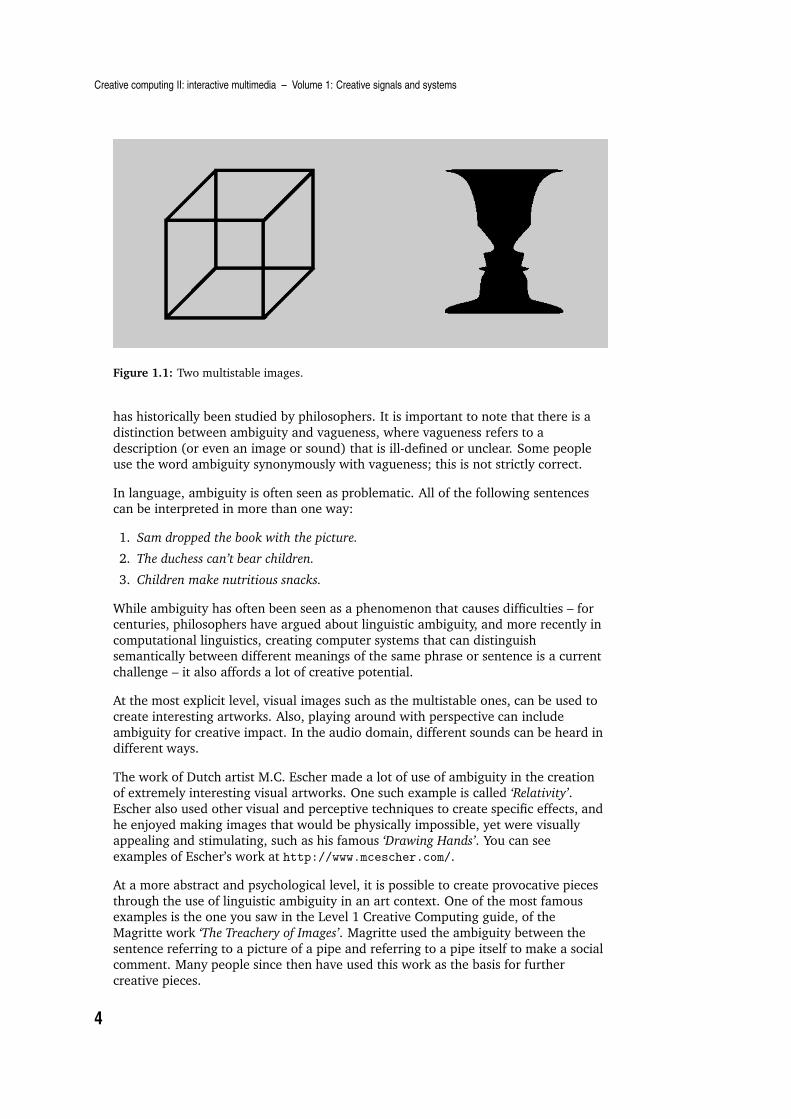
A direct example of ambiguity is demonstrated by the Gestalt property ofmultistability, which is illustrated in Figure 1.1. This is visual ambiguity, where it is
possible to see one of two images, and to alternate between them.
More generally, ambiguity is the property of allowing, or admitting, more than one
interpretation. It plays an important role in the spoken and the visual domains, and
3
Creative computing II: interactive multimedia – Volume 1: Creative signals and systems
Figure 1.1: Two multistable images.
has historically been studied by philosophers. It is important to note that there is a
distinction between ambiguity and vagueness, where vagueness refers to a
description (or even an image or sound) that is ill-defined or unclear. Some peopleuse the word ambiguity synonymously with vagueness; this is not strictly correct.
In language, ambiguity is often seen as problematic. All of the following sentencescan be interpreted in more than one way:
1. Sam dropped the book with the picture.
2. The duchess can’t bear children.
3. Children make nutritious snacks.
While ambiguity has often been seen as a phenomenon that causes difficulties – forcenturies, philosophers have argued about linguistic ambiguity, and more recently in
computational linguistics, creating computer systems that can distinguishsemantically between different meanings of the same phrase or sentence is a current
challenge – it also affords a lot of creative potential.
At the most explicit level, visual images such as the multistable ones, can be used to
create interesting artworks. Also, playing around with perspective can include
ambiguity for creative impact. In the audio domain, different sounds can be heard indifferent ways.
The work of Dutch artist M.C. Escher made a lot of use of ambiguity in the creationof extremely interesting visual artworks. One such example is called ‘Relativity’.
Escher also used other visual and perceptive techniques to create specific effects, and
he enjoyed making images that would be physically impossible, yet were visuallyappealing and stimulating, such as his famous ‘Drawing Hands’. You can see
examples of Escher’s work at http://www.mcescher.com/.
At a more abstract and psychological level, it is possible to create provocative pieces
through the use of linguistic ambiguity in an art context. One of the most famousexamples is the one you saw in the Level 1 Creative Computing guide, of the
Magritte work ‘The Treachery of Images’. Magritte used the ambiguity between the
sentence referring to a picture of a pipe and referring to a pipe itself to make a socialcomment. Many people since then have used this work as the basis for further
creative pieces.
4

Exercises
1.5 Summary and learning outcomes
This introductory chapter focused on perception: what it is and different views on
how perception works at a cognitive level. We also looked at the role that perceptionhas in the creation of artworks.
With a knowledge of the contents of this chapter and its directed reading andactivities, you should be able to:
describe some of the issues regarding how physical stimuli and perceived
entities connect
discuss different views on how perception works
explain what is meant by ambiguity, and give examples of ambiguity in visual
and linguistic contexts
discuss the role of abstraction in how we perceive entities in the world.
1.6 Exercises
1. What is cognition? What is cognitive science? What is artificial intelligence?
How do these areas relate to each other and to psychology?
2. In linguistics, ambiguity can occur in different places. Give examples of each of:
lexical ambiguity
syntactic ambiguity
structural ambiguity
semantic ambiguity.
3. What is musical ambiguity? Find some examples of this.
4. What is abstraction? What role does abstraction have in how we understandlanguage? What role does abstraction have in how we experience visual art, or
music?
5. There is an excellent article on the use of Gestalt principles in user interfacedesign, at http://www.interaction-design.org/encyclopedia/
gestalt principles of form perception.html.
Read the article and then develop a visual image, such as a book cover, a webpage, an advertisement, or some other media item, that incorporates one or
more of the Gestalt principles or other principles of perception. You need not
restrict yourself only to principles mentioned in the article. Write a short essaythat describes which principles you have used and in what way, in your image.
6. Find out more about the work of Escher. Create a piece of digital art or music
that connects in some way with one or more of Escher’s artworks. Write a briefaccompanying description and critique of your work. You may use any software
you like for this.
7. Earlier in this chapter, we noted that Western culture emphasises the visual.Discuss this claim, and present evidence that either backs it up or challenges it.
5

Creative computing II: interactive multimedia – Volume 1: Creative signals and systems
6
Chapter 2
Creative signals
Supplementary reading
Foley, J.D., A. van Dam and others Introduction to Computer Graphics. (Reading, Mass.; Wokingham: Addison Wesley,
1997) [ISBN 0201609215].
Oppenheim, A.V. and A.S. Willsky with S. Hamid Nawab Signals and Systems. (Upper Saddle River, N.J.; London:
Prentice Hall, 1997) [ISBN 0138147574]. Introductory parts of Chapters 1 and 2.
2.1 Introduction
This subject takes signals as the fundamental mechanism for the creation of art, andwe look first at the basic sources of signals – with a focus on sound and images. We
look primarily at signals in the form of waves and patterns. Once we have
understood the fundamentals of waves, and the mathematical ways that are used todescribe them, we will look at ways to manipulate them and ways to analyse
different waveforms, thereby creating new waves and hence new signals.
What is a signal? It can be viewed from many perspectives, including being:
a medium or entity through which communication happens
a physical or biological stimulus
a (mathematical) function
a cultural entity
a subtle message
a wave, or waveform, that is emitted.
2.2 Waves
Both light (which is what enables us to see) and sound (which is what enables us tohear) are periodic waveforms. Light also has a particle representation, which carries
information too, but we focus on the wave aspect of light in this subject.
We will see in later chapters that any periodic waveform can ultimately be
represented by a combination of sine waves,1 so it is important that you understandwhat a sine wave is, what properties it has, and how it is described mathematically.
We’ll also see, in volume 2 of this guide, details of the way that these two kinds of
waveforms interact with our ears and our eyes.
1This discovery is due to Joseph Fourier, a French mathematician of the 18th century.
7
Creative computing II: interactive multimedia – Volume 1: Creative signals and systems
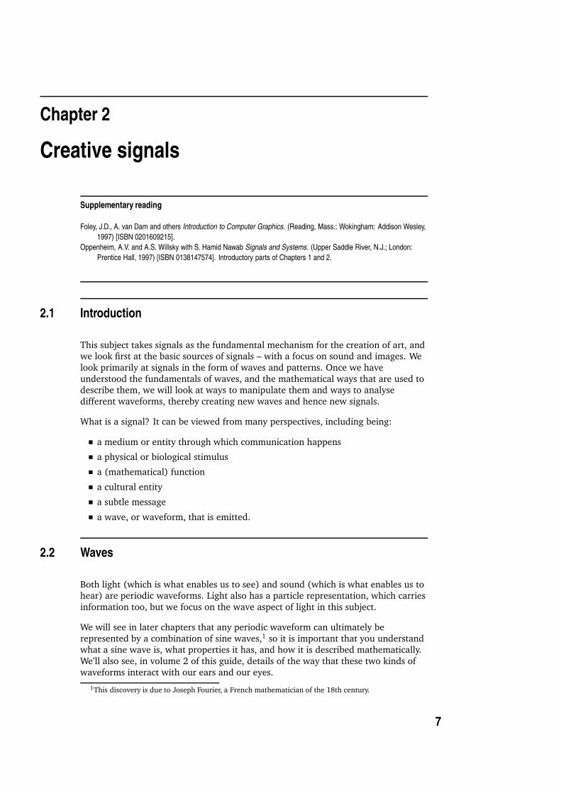
Figure 2.1 shows a sinusoidal waveform; all sinusoids have a similar shape, and thevalues of frequency, wavelength, amplitude and phase may change. There are two
interactive tutorials to be found, athttp://hermes.eee.nott.ac.uk/teaching/cal/h61sig/sig0001.html and
http://www.music.sc.edu/fs/bain/atmi02/wt/sine/index.html, which will
help you understand some of the properties of sinusoids. The latter also has a facilitythat allows you to hear what a sinusoidal waveform sounds like.
Sinusoids can be represented mathematically in the form of a function; mostcommonly the function describes amplitude with respect to angle, and it is this that
is related to the periodicity. The period is the length (usually of time) of one cycle; in
terms of the signals we are looking at, this might be the cycling through all theangles of one full rotation of a circle. The angle may vary from 0◦ to 360◦, or 0
radians to 2π radians. Commonly, the frequency of a sinusoidal waveform is taken tobe the number of oscillations or cycles per second.
Figure 2.1: Sine wave showing degrees and radians.
Learning activity
What is a radian? What is the relationship between radians and degrees?
Construct a diagram that shows the equivalence between radians and degrees. Use Processing to turn
your diagram into something visually interesting.
2.3 Signal processing
Signal processing involves the manipulation of signals, and usually takes signals to
be in the form of waves. In the rest of this subject guide, we will look in much moredetail at the various parts of this signalling arrangement. Although signal processing
applies to analogue as well as to digital signals, we focus in this subject on the
digital. Signal processing can be used as the basis of a wide range of applications,from scientific and engineering through to sound and visual art.
8

Signal processing
2.3.1 RADAR
RADAR was one of the earliest applications of signal processing theory. RADAR
stands for radio detection and ranging – radio waves were used to detect both thepresence of and distance away from an object. The radio waves are signals that are
sent out in a particular direction. They have properties, including the fact that if theyencounter an object they will change their shape and the direction in which they are
moving. Also, they take a certain amount of time to travel through the air. So, many
things can be measured and many things can be calculated. It was thisunderstanding that led to the ability to use signal processing for detecting the
presence of objects, without being able to actually ‘see’ them.
Here is one example of how it works, in a very simplified fashion: electromagnetic
radiation is sent out. This radiation is modelled by waves, so we can think of theradiation as being waves. The waves encounter objects in their path, and some of
the radiation bounces back. The RADAR system detects this radiation that has been
bounced back. Because waves travel at a known speed through air, it is possible totell how far away from the RADAR system the object that caused the bouncing is.
Many other measurements can be made to determine factors other than the presence
of an object, and its distance from the emitter. However, the earliest RADAR systemswere developed for just this purpose: being able to silently detect the presence of
enemy planes in the air.
2.3.2 Audio signals
An early use of audio signal processing was in radio, which was in the analogue
domain for a long time. The development of digital radio is relatively recent.
Learning activity
How does analogue radio work? What do the terms AM, FM, SW and LW mean, and what do they refer to
in terms of the radio signal?
How does digital radio differ from analogue radio?
Speech and sound signal processing has been of interest in the digital world sincethe 1960s. An example of an audio signal is shown in Figure 2.2; sound signals can
be visualised in a number of ways, which include the use of colour and light
intensity, and the more traditional use of waveforms as indicated in the bottomsection of the figure.
Audio signal processing covers music, speech, and other sound, and areas of interestinclude digital processing, manipulation of music and audio recordings, speech
recognition, and speech generation. More recently, signal processing has beenapplied to the recognition and identification of music.
Learning activity
Find out what you can about Hermann von Helmholz. In particular, find out what his contributions have
been to audio processing. What is a Helmholz resonator?
9

Creative computing II: interactive multimedia – Volume 1: Creative signals and systems
Figure 2.2: Speech signals.
2.3.3 Image signals
One form of image processing is the application of signal processing to images, and
it can be considered especially within digital image processing. Simply taking a
colour image and turning it into a black and white image is a type of signalprocessing. In this case, the signals for the image are the colour and light signals at
each pixel, and the processing involves processing each of these to produce thedesired output. There is a wide range of operations that can be applied to image
signals to produce desired outputs and effects, from resizing to blurring. You saw
some of these in Processing in Level 1. The focus in Level 2 is on signals and whatcan be done to them.
2.3.4 Visual art and music
Evolutionary and generative art can be viewed as an application of signal processing.In the Level 1 subject guide, you saw examples of image transformations using
things like rotation and scaling, as well as texture mapping. Signal processing
techniques can be applied to create interesting and novel images, and images thatmove and grow, as in the work of Karl Sims, who was an early exponent in this field.
William Latham is an artist who used digital techniques to model evolutionary
processes, thereby creating distinctive artworks, as well as biologically relevant
10

Signal definition
images, as demonstrated in Figure 2.3.
Figure 2.3: Image from William Latham’s Mutator.
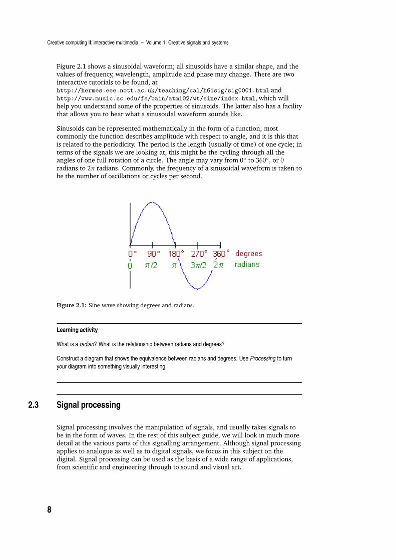
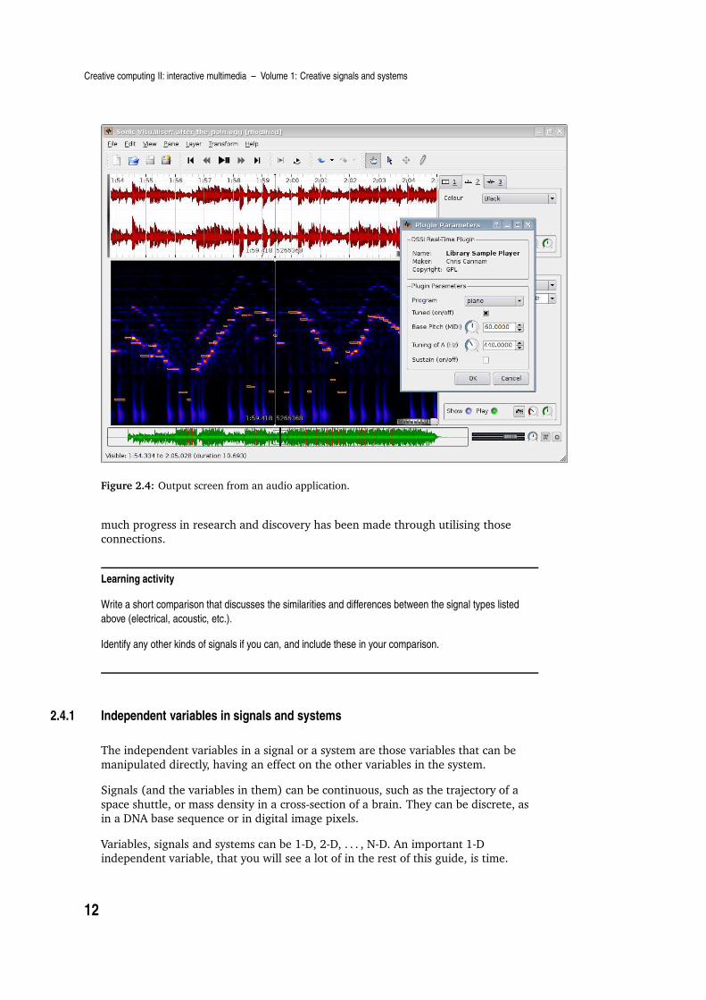
Figure 2.4 shows a screen of a digital music interface. Processing music as a digital
signal allows us to analyse music from a different perspective, that examines themuch smaller elements that then contribute to the overall whole. In Volume 2 of this
guide, you’ll see systems (soundspotter and videospotter), which apply a signal
processing approach to the retrieval of specific information from a large bank ofdata.
As well as analysing music, the application of signal processing allows the creationand generation of novel music, such as in the work of John Cage.
Learning activity
Find more examples of musicians and artists who make use of signal processing explicitly in their work.
Describe how they do this, and what is unique and interesting about it.
2.4 Signal definition
Signals are functions of independent variables that carry information.
For example:
electrical signals – voltages and currents in a circuit
acoustic signals – audio or speech signals (analogue or digital)
video signals – intensity variations in an image (e.g. a CAT scan)
biological signals – sequence of bases in a gene.
You’ll see more on signals in the context of sound and image analysis, and sound andimage creation, in the rest of this subject. However, it is important to appreciate that
there is theory about signals that cuts across a number of different subject areas, and
11
Creative computing II: interactive multimedia – Volume 1: Creative signals and systems
Figure 2.4: Output screen from an audio application.
much progress in research and discovery has been made through utilising thoseconnections.
Learning activity
Write a short comparison that discusses the similarities and differences between the signal types listed
above (electrical, acoustic, etc.).
Identify any other kinds of signals if you can, and include these in your comparison.
2.4.1 Independent variables in signals and systems
The independent variables in a signal or a system are those variables that can be
manipulated directly, having an effect on the other variables in the system.
Signals (and the variables in them) can be continuous, such as the trajectory of a
space shuttle, or mass density in a cross-section of a brain. They can be discrete, asin a DNA base sequence or in digital image pixels.
Variables, signals and systems can be 1-D, 2-D, . . . , N-D. An important 1-Dindependent variable, that you will see a lot of in the rest of this guide, is time.
12

Exercises
We distinguish between:
Continuous-Time (CT) signals: x(t), t →continuous values
Discrete-Time (DT) signals: x[n], n →integer values only.
Discretisation involves taking a continuous time signal and turning it into a discrete
time signal.
Learning activity
How would you go about discretising a continuous signal? What is quantisation? How would you go about
quantising a signal?
Learning activity
For the signals in Section 2.4 above, which are the independent variables?
What is a dependent variable? Give some examples of dependent variables in relation to the first part of
this learning activity.
2.5 Summary and learning outcomes
In this chapter we saw that sound and image, among many other things, can be
viewed as signals. This is the approach taken in the rest of the volume, and this
chapter has formed an introduction to the approach. In subsequent chapters, youwill learn in more detail about different aspects of signals and signal processing, and
how to apply these.
With a knowledge of the contents of this chapter and its directed reading and
activities, you should be able to:
discuss different types of signals
describe the importance of waves in signal processing
distinguish between discrete and continuous signals
convert between angles in degrees and radians; and discuss how sine and cosine
waves can be represented over time
give examples of the application of signal processing in the making of artworks.
2.6 Exercises
1. For each of the different views of signals listed at the very start of this chapter,give a short paragraph explaining what is meant by that entity being a signal.
Include examples in your response.
2. Cosine waves and sine waves are both examples of sinusoidal waveforms. Whatis the relationship between sine and cosine waves?
13

Creative computing II: interactive multimedia – Volume 1: Creative signals and systems
3. What is the independent variable in a sinusoidal waveform?
4. What do the functions cos(x) and sin(x) do? What is x in these functions?
5. What is the relationship between frequency and periodicity?
6. Find at least three different examples of displaying of audio signals. Describe
how each of them works, and compare them in terms of their effectiveness andthe advantages and disadvantages of the approach taken.
14

Chapter 3
Signals
Essential reading
Eaton, J.W. GNU Octave Manual. (Bristol: Network Theory, 1996) [ISBN 0954161726]. (This is also
available online in HTML form at
http://www.gnu.org/software/octave/doc/interpreter and in texinfo source format in
the Octave source code distribution.)
Recommended reading
Oppenheim, A.V. and A.S. Willsky with S. Hamid Nawab Signals and Systems. (Upper Saddle River, N.J.; London:
Prentice Hall, 1997) [ISBN 0138147574] Chapter 1.
3.1 Introduction
In this chapter you will learn about the fundamental concepts of signals as they areunderstood by the engineering profession. To assist in the understanding of signals,
and in the next chapter, ‘Systems’, it is useful to get some direct experience of
constructing and manipulating them.
Digital multimedia systems are built upon a class of signal and system buildingblocks called discrete-time signal processing, or digital signal processing (DSP). DSP
is a branch of engineering that is concerned with the analysis and design of signals
and systems for everyday applications, such as: radar, satellite communication,seismic monitoring, rocket guidance systems and, the subject of this guide, digital
multimedia.
Signals are built out of fundamental units that are combined to make more
complicated signals using basic mathematical operations. Therefore, this chapter
introduces the fundamental building blocks of DSP and methods to construct andmanipulate signals.
3.2 Octave
Octave is an open-source mathematics and engineering tool that was written by
John Eaton and it is maintained as part of the free software foundation’s GNUproject; as such, it will be available to use for free well into the future. Octave is
useful for the construction, manipulation and visual display of signals. It can also be
used for displaying images, audio and video, that are manipulated using DSPtechniques. In later chapters you will learn how to perform signal manipulations in
15
Creative computing II: interactive multimedia – Volume 1: Creative signals and systems
Octave; in the current chapter you will learn how to install and run Octave, and howto start constructing signals out of fundamental DSP units.
3.2.1 Installing Octave
You will first need to obtain the latest version of Octave. As an open-source project,Octave is freely available on the Internet. If your operating system has a package
manager (such as fink on Mac OSX or Synaptic Package Manager in Ubuntu Linux)then you should use the package manager to install the latest version of Octave.
Otherwise you can download Octave directly from:
http://www.gnu.org/software/octave/
At the time of writing, the latest version of Octave is 3.0.1; you should download orinstall at least this version or a later (stable) release if available.
In addition to Octave you will need to install GnuPlot and ImageMagick for plottingand image graphics. Again, if you have a package manager it is likely that the
additional packages were automatically installed when installing Octave. However, if
you do not have a package manager you can obtain both of these packages freelyfrom the Internet:
http://www.gnuplot.info
http://www.imagemagick.org
3.2.2 Installing for different operating systems
Octave’s primary support is for the Linux operating system, so if you are using that,
it is likely that your installation will be straightforward.
Some versions of Windows present problems for Octave, in which case you are
recommended to download Cygwin – -a version of Linux that runs on Windows
systems – -and run Octave within that.
For students using Mac, you are advised to go to http://pdb.finkproject.org if you
encounter any problems with your installation.
Please also note that the plotting examples might look different from the ones in this
guide, depending on which version of Octave you are using. What is important isthat your plots illustrate to you the concepts, and that you become competent in
using Octave to test them out.
3.2.3 Running Octave
Once you have installed Octave you can test it by opening a terminal window and
typing the Octave command.
shell%1>octave
Octave will start up and will print some information about the version and the
copyrights of the software. For example, you might get the following message:
16
Octave
GNU Octave, version 3.0.1 (i486-pc-linux-gnu).
Copyright (C) 2006 John W. Eaton.
This is free software; see the source code for copying conditions.
There is ABSOLUTELY NO WARRANTY; not even for MERCHANTIBILITY or
FITNESS FOR A PARTICULAR PURPOSE. For details, type ‘warranty’.
Additional information about Octave is available at
http://www.octave.org.
Please contribute if you find this software useful.
For more information, visit http://www.octave.org/help-wanted.html
Report bugs to <[email protected]> (but first, please read
http://www.octave.org/bugs.html to learn how to write a helpful
report)
You are now presented with Octave’s interactive shell which allows you to entercommands and display the results of mathematical operations. The interactive
nature of Octave is an advantage over languages that require compilation, such as
Java, because the response to entering your code is immediate.
3.2.4 Using Octave
Octave can manipulate numbers that are organised into convenient containers called
vectors and matrices. In Octave, all numbers are actually matrices, but the userdoesn’t know this until they need to use matrices.
Scalars
A scalar is a single numeric quantity, such as the numbers 3, −6.3 and the irrational
pi. When you type these values at the Octave prompt, they will be evaluated asexpressions and their values returned as answers:
octave:> 3
ans = 3
octave:> -6
ans = -6
octave:> pi
pi = 3.1416
Note that the last of these three inputs evaluated a pre-defined constant: pi. Just as
in the other programming languages that you have used in your studies, we candefine a variable to contain a value. Octave is not a typed system, so variables do not
have to be declared and assigned types explicitly; we can simply define a variable by
assigning it a value:
octave:> a = -100
a = -100
octave:> b = pi
b = 3.1416
octave:> aLongVariableName = 10
aLongVariableName = 10
17
Creative computing II: interactive multimedia – Volume 1: Creative signals and systems
Scalar operations
The same mathematical operations that you have used in Java and other
programming languages are also available in Octave. There common operations ofaddition, subtraction, multiplication and division can be entered directly at the
command prompt and Octave will evaluate them:
octave:> 4.5 + 9.6 * 2
ans = 23.7
octave:> ( 4.5 + 9.6 ) * 2
ans = 28.2
octave:> ( 4.5 + 9.6 ) / 2
ans = 7.05
octave:> ( 4.5 + 9.6 ) ^ 2 / 2
ans = 99.405
The order of precedence of operators is similar to that of Java, with multiplication
taking precedence over addition, and division taking precedence over multiplication.The order of operation is altered with the use of parentheses as in the above
examples. In the last example the ^ operator was used to perform exponentiation;
raising the expression in the parentheses to the power 2 thus taking its square.
Mathematical operations can also be performed on variables in the same manner. Inthe following examples the variables defined above are used in mathematical
expressions:
octave:> ( a*a + b ^3 ) / aLongVariableName
ans = 1003.1
octave:> 2*pi
ans = 6.2832
octave:> pi/2
ans = 1.5708
Mathematical functions
Octave provides a comprehensive set of mathematical functions such as sin(),cos(), tan(), exp(), asin(), acos(), atan(), min(), max(), mean().
Functions are expressions that return a value given one or more input arguments.The following examples illustrate some of the more common functions:
octave:> cos(0)
ans = 1
octave:> sin(pi)
ans = 1.2246e-16
octave:> sin(pi/2)
ans = 1
octave:> exp(1)
ans = 2.7183
octave:> tan(pi/2)
ans = 1.6332e+16
The functions cos(), sin() and tan() are the familiar trigonometric functions that
18

Octave
you may have used either in Java or on a calculator. They accept a scalar argumentin the range [0 . . .2π] and return the value of the function for the given argument.
Note that the values for sin(pi) and tan(pi/2) are not exact: the mathematicallycorrect values of these functions for the given arguments are 0 and Infinity (or ∞)
respectively. Here, as with all mathematical operations, Octave reports the value of
the function to within the floating-point numerical accuracy of the host system. Thevalues are not exact because of finite floating-point precision; the same is true in the
Java programming language.
The exp() function is the exponential function which raises the natural exponent e,
often called the Euler number, to its argument. Thus, exp(1) returns the identity of
the natural exponent, to a fixed number of decimal places, in this case 4 decimalplaces (2.7183). To see more of the decimal places of this irrational number use the
format long command:
octave:> format long
octave:> exp(1)
ans = 2.71828182845905
To return to the default short format use the command format short.
All of the functions in octave have built-in help available. To access the help use
‘help functionname’, for example:
octave:>help sin
Relational and conditional operators
Just like Java, Octave also has basic programming constructs such as relational
(<,>,<=,>=,==,), conditional (if(...) endif; switch..case) and control
operations (for(...) endfor; while(...) endwhile;. We may use Octave by
writing a script, storing it in a file, and calling the script by name to access itsfunctionality.
Learning activity
Type the following into your text editor; for example gedit, wordpad or emacs:
for k = 10:-1:0
if(k>0)
100/k
else
printf(’What will happen if we divide by zero?’)
100/k
endif
endfor
Do not worry about the syntax for now; but most of this code should look familiar to you. It is very similar to
Java except it does not use braces ‘{}’ to delimit code blocks. Instead, blocks of code are delimited bykeywords such as for (...) endfor and if ...endif as in many Unix-style scripting
languages.
19
Creative computing II: interactive multimedia – Volume 1: Creative signals and systems
Now save the file using the name myscript.m in a CC227 working directory, say, ~/CC227/octave.
The symbol ~ means your HOME directory. The extension .m is used by Octave to locate script and
function files.
You will first need to make a directory to store your scripts. Do this either from the desktop of your operating
system, from a terminal or even in Octave:
octave:> mkdir(’~/foo/bar’)
ans = -1
Only one directory at a time can be created; here, since ~/foo did not exist an error is returned (−1) whentrying to make the bar directory within it.
Instead, we must create each new directory separately:
octave:> mkdir(’~ /CC227’)
ans = 0
octave:> mkdir(’~ /CC227/octave’)
ans = 0
The return value, 0, indicates that all is well with the new directories. When you have saved myscript.m
you will need to tell Octave where to find it so that you can use it. To do this, use the addpath command:
octave:>addpath(’~ /CC227/octave’)
Octave’s path command will display all the directories that Octave will look in to find scripts and data files
that you might request at the command prompt.
octave:>path
Octave’s search path contains the following directories:
~/CC227/octave
.
/usr/lib/octave/2.1.73/site/oct/i486-pc-linux-gnu//
/usr/lib/octave/site/oct/api-v13/i486-pc-linux-gnu//
/usr/lib/octave/site/oct/i486-pc-linux-gnu//
/usr/share/octave/2.1.73/site/m//
/usr/share/octave/site/api-v13/m//
/usr/share/octave/site/m//
/usr/lib/octave/2.1.73/oct/i486-pc-linux-gnu//
/usr/share/octave/2.1.73/m//
/usr/local/share/octave/site-m//
Do not worry about the long list of directories, you are most interested in the ones at the top. The single “.”
refers to the current working directory which can be displayed using the command pwd:
octave:> pwd
/home/mkc/CC227/octave
If all has gone well, you should now be able to execute your script from the command line:
octave:>myscript
ans = 10
20
Octave
ans = 11.111
ans = 12.500
ans = 14.286
ans = 16.667
ans = 20
ans = 25
ans = 33.333
ans = 50
ans = 100
What will happen if we divide by zero?
warning: division by zero
ans = Inf
What happened at the end of the script?
Is the last value a numeric?
Octave supports scripts, as in the example above, which accept no arguments and do not return a value. A
script can output a value to the screen, such as in your example above.
To support input arguments and return values Octave also allows user-defined functions. Functions are,
essentially, scripts with an extra keyword to define a function, and they are able to accept and return
arguments.
Make a new text file in your Octave directory called myfunction.m:
function y = myfunction(n)
for k = n:-1:0
if(k>0)
y = 100/k
else
printf(’What will happen if we divide by zero?’)
y = 100/k
endif
endfor
endfunction
The Octave path was already set above; so you may now type the following at the command line:
octave:>myReturnValue = myfunction(5)
y = 20
y = 25
y = 33.333
y = 50
y = 100
What will happen if we divide by zero?
warning: in /home/mkc/src/octave/myfunction.m near line 7, column 8:
warning: division by zero
y = Inf
myReturnValue = Inf
Explain why the number contained in myReturnValue is the last value computed by myfunction.m.
21

Creative computing II: interactive multimedia – Volume 1: Creative signals and systems
Vectors
So far, the scalar operations that you have executed in Octave have been very similar
to the numerical computations that you have used in other programming languages.The power of Octave comes in combining many scalar values into ordered lists,
called vectors and matrices. Octave’s operations upon vectors and matrices makeprogramming for signals and systems much easier than it would be in languages
such as Java.
A vector is simply a list of scalar values such as [2 4 6 8 10] and [exp(1) 23.7 42
-pi]. A vector is defined with the use of the square brackets [ and ]. The following
are examples defining vectors in Octave:
octave:> [exp(1) 23.7 42 -pi]
ans =
2.7183 23.70 42.00 -3.1416
octave:> [pi pi/2 pi/3 pi/4 pi/5 pi/6 pi/7 pi/8 pi/9]
ans =
Columns 1 through 8:
3.14159 1.57080 1.04720 0.78540 0.62832 0.52360 0.44880 0.39270
Column 9:
0.34907
In the first example, a vector was constructed using both scalar literals and
functions. The functions are evaluated and the results inserted into the vector. The
vector is then a fixed set of numbers. In the second example, the pre-definedconstant pi was used to construct every element of the vector. The result is a vector
of nine elements with values that spill over two lines. When this happens, duringprinting to the screen, Octave informs the user which columns appear on each line.
The term column refers to the number of elements that the vector contains if it isoriented as a row vector as in the examples above. Vectors have either one row and
multiple columns of values, or one column and multiple rows. The orientation of a
vector determines whether its values are organised in rows or columns.
To find out whether a vector is a row or a column vector you can use Octave’s
size() command:
octave:> size([-1 0 1 2 3 4 5])
ans =
1 7
The size command returns the number of rows and columns in a vector. In this
example, the command has resulted in a response of 1 7 for row and column
respectively, indicating that the resulting vector is a row vector.
To make a column vector you can enter the values one row at a time:
octave:> [
> -1
> 0
> 1
> 2
> 3
> 4
> 5]
22

Octave
ans =
-1
0
1
2
3
4
5
Notice that the resulting values are now listed as a single column.
Conveniently, Octave keeps the last computed value in an automatic variable calledans; in this case a column vector. The size function can be called with ans as an
argument to find out the number of rows and columns of the last computed vector:
octave:> size(ans)
ans =
7 1
Now Octave reports that there are 7 rows and 1 column; so this is a column vector.
The orientation of a vector is very important. The process of changing orientation is
a fundamental operation in Octave called transposition; transposition of a vector isobtained with a special operator “ ’ ”.
In the following examples we transpose a row vector into a column vector, and acolumn vector into a row vector. Just as with scalars, you can assign vectors to
variables. There is nothing special that needs to be done; Octave treats scalars and
vectors in the same manner for variable assignment:
octave:> a = [-1 0 1 2 3 4 5]
a =
-1 0 1 2 3 4 5
octave:> b = [-1 0 1 2 3 4 5]’
b =
-1
0
1
2
3
4
5
octave:> aSize = size( a )
aSize =
1 7
octave:> bSize = size( b )
bSize =
7 1
Notice how the number of rows and columns is exchanged with the use of the ’
operator.
Another special operator enables vectors to be defined as sequences of numeric
23

Creative computing II: interactive multimedia – Volume 1: Creative signals and systems
values, without having to list the entire sequence. The colon operator : was usedabove in the myfunction.m function; it is an iterator that generates a list of values
between a start value and an end value:
octave:>[1:10]
ans =
1 2 3 4 5 6 7 8 9 10
octave:> [10.5:20.4]
ans =
10.5 11.5 12.5 13.5 14.5 15.5 16.5 17.5 18.5 19.5
In the above two examples, the start and end values are traversed in order in stepsizes of 1.0, the default increment for colon operator iteration.
Learning activity
In the second example above, the value 20.4 is not reached. Can you see why?
To change the step size of the iteration Octave has a syntax using two colon
operators:
octave:> [10.5:.9:20.4]
ans =
Columns 1 through 10:
10.5 11.4 12.3 13.2 14.1 15.0 15.9 16.8 17.7 18.6
Columns 11 and 12:
19.5 20.4
Learning activity
Here the value 20.4 is reached. Can you see why?
In this example, the direction of the iterator is reversed by the use of a negative
increment:
octave:> myVector = [10:-1:1]’
myVector =
10
9
8
7
6
5
4
3
2
1
The increment argument to the colon operator can have any real numeric value. In
this example the resulting vector was transposed to a column vector using the
transpose operator ’.
24

Octave
Learning activity
Try reversing the positions of 10 and 1 in the above example. Explain the output that you see.
Vector arithmetic operations
The same mathematical operations are available for vectors as for scalars. First, wecan apply the basic operations of addition, subtraction, multiplication and division
between vectors and scalars:
octave:> aVec = [ 0 : 0.1 : 1 ]
aVec =
Columns 1 through 8:
0.0 0.1 0.2 0.3 0.4 0.5 0.6 0.7
Columns 9 through 11:
0.8 0.9 1.0
octave:> aVec + 1
ans =
Columns 1 through 10:
1. 1.1 1.2 1.3 1.4 1.5 1.6 1.7 1.8 1.9
Column 11:
2.0
octave:> aVec * 10
ans =
Columns 1 through 8:
0.0 1.0 2.0 3.0 4.0 5.0 6.0 7.0
Columns 9 through 11:
8.0 9.0 10.0
octave:> aVec - 1
ans =
Columns 1 through 8:
-1.0 -0.9 -0.8 -0.7 -0.6 -0.5 -0.4 -0.3
Columns 9 through 11:
-0.2 -0.1 0.0
octave:> aVec / 0.1
ans =
Columns 1 through 8:
0.0 1.0 2.0 3.0 4.0 5.0 6.0 7.0
Columns 9 through 11:
8.0 9.0 10.0
The following examples consist of arithmetic operations between two vectors:
octave:> bVec = [ 1 : -0.1 : 0 ]
bVec =
Columns 1 through 8:
1.0 0.9 0.8 0.7 0.6 0.5 0.4 0.3
Columns 9 through 11:
0.2 0.1 0.0
octave:> aVec + bVec
ans =
25
Creative computing II: interactive multimedia – Volume 1: Creative signals and systems
1 1 1 1 1 1 1 1 1 1 1
octave:> aVec - bVec
ans =
Columns 1 through 8:
-1.0 -0.8 -0.6 -0.4 -0.2 0.0 0.2 0.4
Columns 9 through 11:
0.6 0.8 1.0
The operations of vector addition and vector subtraction simply perform the scalaroperations of addition and subtraction independently on each pair of vector
elements taken in order.
Learning activity
What happens if you add, or subtract, two vectors of different lengths? Why does this happen?
What happens if you transpose one of two vectors of the same length and perform addition or subtraction?
What happens if you transpose both vectors? Can you explain the result?
The rule for adding, or subtracting, pairs of vectors is that they must have the same
dimensionality. That is, they must both be either row vectors or column vectors and
they must have the same number of elements. Before performing vector addition orsubtraction it is often useful to use the size() command, to make sure that the
vectors are compatible with the rules of vector arithmetic.
Vector indexing
Octave provides access to the individual elements of a vector variable usingparentheses: (). The ordinal position of the element that is required is supplied as
an argument, as if the vector variable were itself a function. For example:
octave50>a = [1 1 2 3 5 8 13 21 34]
>a(4)
ans = 3
>a(9)
ans = 34
>a(0)
error: invalid vector index = 0
>a(10)
error: invalid vector index = 10
Note that the indexing is one-based, not zero-based as it is in Java. This can lead to alot of confusion when moving from Java to Octave, so it is best to take extra care
when writing index code in Octave.
The argument supplied for vector indexing can be another vector. The elements of
the inner index vector are the positions in the outer vector to access:
octave:> a([2 4 6 8])
ans =
1 3 8 21
26

Octave
octave:> a([3 5 7 9])
ans =
2 5 13 34
octave:> a([1:2:9])
ans =
1 2 5 13 34
In the last example, the colon notation was used to construct an index vector
starting at 1 with increment 2 and ending at 9. This example demonstrates howvectors can take on different roles depending on how they are used. Mastery over
vectors and their notation in Octave will be necessary for understanding the
concepts of signals and systems and how they can be implemented in Octave.
Learning activity
For each of the following, find at least three ways to construct the vector: (Hint: you can use direct
construction, the colon operator and arithmetic operators.)
even numbers from 22 to 56
odd numbers from -17 to -39
the Sine function for values pi/8, 2*pi/8, 3*pi/8, 4*pi/8
the eighth through 10th powers of 2
a single vector consisting of the integers 1 through 5 forwards and then backwards.
Vector multiplication
You should already be familiar with vector and matrix multiplication; here we revisit
the principles of vector multiplication in the context of Octave.
Given the above examples it may seem intuitive that two vectors should be
multiplied in the same way as addition. Try multiplying two vectors that are of the
same dimensionality:
octave:> aVec * bVec
error: operator *: nonconformant arguments (op1 is 1x11, op2 is
1x11)
error: evaluating binary operator ‘*’ near line 50, column 6
What has happened? The dimensionality of the vectors is the same; yet Octave has
given a nonconformant arguments error.
The operation of vector multiplication is not the same as element-wise scalar
multiplication. Instead, it has a special meaning that is unique to vectors. When twovectors are multiplied, the elements are taken from the columns of the first vector
and the rows of the second vector. In other words, the two vectors must be in
different orientations. Let us see what happens when we multiply two vectors ofequal lengths – i.e. the same number of elements – but transpose the second vector
to be a column vector:
27

Creative computing II: interactive multimedia – Volume 1: Creative signals and systems
octave:> aVec * bVec’
ans = 1.65
The result is a single number: 1.65. This number is obtained by first multiplying eachelement of the first vector with each element of the second and then summing all the
values to get a single number. This is a fundamental operation of Linear Algebra,which is the branch of mathematics that Octave uses to represent numerical
computations.
The operation of multiplying two vectors produces either a scalar or a whole set of
new vectors, called a matrix, depending on the orientation of the two arguments.
This algebra is non-commutative; this means that if we change the order of themultiplication we usually get a different answer. This is different from scalar
multiplication which is commutative, so changing the order of a multiplication doesnot affect the result and the same value is obtained.
Learning activity
There are some instances where matrix multiplication can be commutative. Give some examples where this
is the case.
Some examples of vector multiplication in Octave follow:
First, let us define two vectors of the same length but in different orientations.
octave:> a = [0 1 2]
a =
0 1 2
octave:> b = [3 4 5]’
b =
3
4
5
octave:> size(a)
ans =
1 3
octave:> size(b)
ans =
3 1
The above example defines a row vector and a column vector. The size() function
is used to discover the dimensions of each of the vectors: size(a) == [1 3] and
size(b) == [3 1]. If we take the number of rows of the first vector, a and thenumber of columns of the second vector, b, the two resulting values inform us of the
dimensionality of the output: in this case it will be [1 1], which means one row and
one column, which is simply a scalar.
Each column of the first vector is multiplied by each row of the second and the
resulting answers are summed to yield the vector multiplication result. Using vectorindexing we can generate the result manually:
octave:> a(1)*b(1) + a(2)*b(2) + a(3)*b(3)
ans = 14
28

What are signals?
Here, each pair of elements was taken from the two vectors in turn and added tomake a final value, 14. This is the value that we obtain if we multiply these two
vectors:
octave:> a*b
ans = 14
A second rule for multiplication is that the second dimension of the first vector must
match the first dimension of the second vector: in this case these dimensions are 3and 3 so all is well. If we transpose one of the vectors then the second dimension of
the first vector and first dimension of the second will not match.
However, if we transpose both of the vectors then we get two vectors that have
dimensionalities [3 1] and [1 3] respectively. The first dimension of the first vector
and the second dimension of the second vector forms a new object that hasdimensionality [3 3]. By the second rule of vector multiplication, the second
dimension of the first vector matches the first dimension of the second vector, 1 and1, respectively, so the operation is permitted. What results, then, is a matrix that is
formed of three column vectors. These column vectors are the first vector [0 1 2]’
scaled by each of the elements of the second vector [3 4 5]:
octave:> a’ * b’
ans =
0 0 0
3 4 5
6 8 10
Note that Octave uses the * symbol for vector and matrix multiplication.
3.3 What are signals?
For the work that follows, we take the view that a signal is a measurement that is
done at regular time intervals. Examples of signals are the temperature reading from
a thermometer taken at hourly intervals, the hours of daylight for each day of theyear, your height measured annually or the number of sounds that you hear between
successive clock ticks. Creative computing is concerned with signals that are
organised for our senses.
You will find it very helpful to look at the introductory chapters of the recommendedreading, or any other book on signal processing, to clarify the basic concepts that
follow.
3.3.1 One-dimensional signals
The examples given above are all one-dimensional signals. That is, they are
functions of one independent variable, time.
Let us construct a real signal using Octave.
29
Creative computing II: interactive multimedia – Volume 1: Creative signals and systems
Learning activity
You will need a clock or watch with a second hand for this activity.
Open Octave, type sig1 = [ without hitting return.
Now, over a ten second period; count the number of sounds you hear between each clock tick and type the
number into Octave followed by a space.
The first click is time 0. The second clock tick will be the first count – i.e. at time index 1. The third clock tick
will yield the second count, at time index 2.
When you reach time index 10, type the last count and then type a ] and hit return.
Octave now has a variable defined called sig1 that provides information about the level of soundactivity in your neighbourhood. There should be 10 samples in your signal. To verify, use Octave’s lengthcommand:
octave:>length(sig1)
ans=10
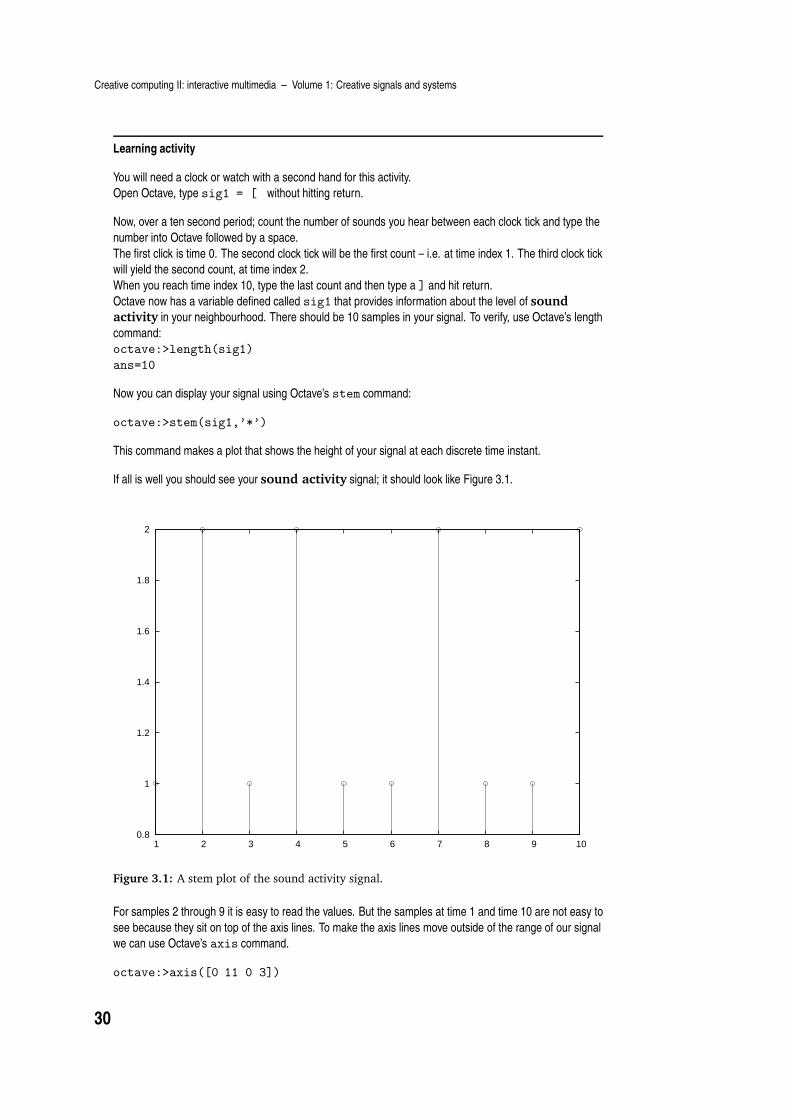
Now you can display your signal using Octave’s stem command:
octave:>stem(sig1,’*’)
This command makes a plot that shows the height of your signal at each discrete time instant.
If all is well you should see your sound activity signal; it should look like Figure 3.1.
0.8
1
1.2
1.4
1.6
1.8
2
1 2 3 4 5 6 7 8 9 10
Figure 3.1: A stem plot of the sound activity signal.
For samples 2 through 9 it is easy to read the values. But the samples at time 1 and time 10 are not easy to
see because they sit on top of the axis lines. To make the axis lines move outside of the range of our signal
we can use Octave’s axis command.
octave:>axis([0 11 0 3])
30
What are signals?
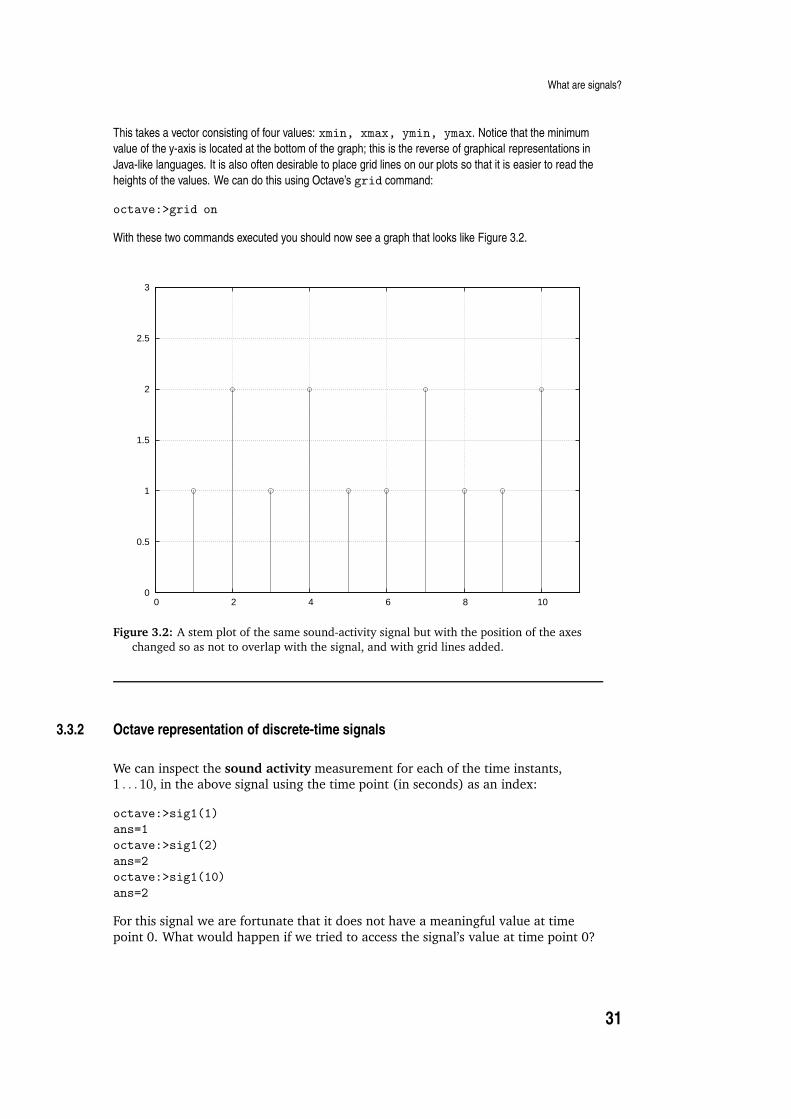
This takes a vector consisting of four values: xmin, xmax, ymin, ymax. Notice that the minimum
value of the y-axis is located at the bottom of the graph; this is the reverse of graphical representations in
Java-like languages. It is also often desirable to place grid lines on our plots so that it is easier to read the
heights of the values. We can do this using Octave’s grid command:
octave:>grid on
With these two commands executed you should now see a graph that looks like Figure 3.2.
0
0.5
1
1.5
2
2.5
3
0 2 4 6 8 10
Figure 3.2: A stem plot of the same sound-activity signal but with the position of the axes
changed so as not to overlap with the signal, and with grid lines added.
3.3.2 Octave representation of discrete-time signals
We can inspect the sound activity measurement for each of the time instants,1 . . . 10, in the above signal using the time point (in seconds) as an index:
octave:>sig1(1)
ans=1
octave:>sig1(2)
ans=2
octave:>sig1(10)
ans=2
For this signal we are fortunate that it does not have a meaningful value at time
point 0. What would happen if we tried to access the signal’s value at time point 0?
31

Creative computing II: interactive multimedia – Volume 1: Creative signals and systems
Learning activity
Try the above. what does Octave do?
Most signals have time indices that do not conveniently line up with Octave’s vector
indexing. The time index must be mapped into a vector index.
To do this we must choose a sample in our signal to act as the zero-time reference
index. This could be vector index 1, or vector index 100, depending on the signal.Time point zero is often used to mean now, rather than simply the beginning of a
signal. The meaning of 0 is determined by the application.
Once a zero-time reference index is chosen we may represent signals that have
negative, zero and positive time index values. In this notation, the zero time index
represents now; negative time indices represent past values of the signal andpositive values represent future values of the signal. This is not to be taken literally;
the concept of the zero time index is simply a reference point for various uses, suchas to relate the time positions of other signals.
Figure 3.3 shows a cosine function that is sampled at nine equally-spaced positions.The spacing of the positions is pi/8, but the time index is discrete, running from 0 to
8.
Here is the signal’s construction in Octave:
octave:>t = 0 : pi/8 : pi
t =
Columns 1 through 8:
0.0 0.39270 0.78540 1.17810 1.57080 1.96350 2.35619 2.74889
Column 9:
3.14159
octave:>sigcos = cos( t )
sigcos =
Columns 1 through 5:
1.e+00 9.2388e-01 7.0711e-01 3.8268e-01 6.1230e-17
Columns 6 through 9:
-3.8268e-01 -7.0711e-01 -9.2388e-01 -1.e+00
octave:>stem(0:length(sigcos)-1, sigcos, ’*’)
octave:>axis([-1 length(sigcos) -1.5 1.5] )
octave:>sigcos( 0 + 1 )
ans = 1
octave:>sigcos( 8 + 1 )
ans = -1
In this example a number of convenient variables are used. The first is the definition
of a vector of time values, t, at which to sample the cosine function. These are thetime points which are distinct from the discrete-time index which runs from
0:length(sigcos)-1. In this case, the time points are related to the discrete-timeindex by a scalar multiplication by pi/8:
octave:>t
t =
Columns 1 through 8:
32

What are signals?
-1.5
-1
-0.5
0
0.5
1
1.5
0 2 4 6 8
Figure 3.3: A cosine signal plotted using Octave’s stem() function. The time interval between
samples is pi/8 but the time index is discrete, running from 0 to the length of the signal
minus 1. This discrete time index is a requirement in digital signal processing.
0.0 0.39270 0.78540 1.17810 1.57080 1.96350 2.35619 2.74889
Column 9:
3.14159
octave:>[ 0 : length(sigcos)-1 ] * pi/8
ans =
Columns 1 through 8:
0.0 0.39270 0.78540 1.17810 1.57080 1.96350 2.35619 2.74889
Column 9:
3.14159
This is the most common form of discrete time index used in signal processing.Finally, when requesting values from the signal vector, the lookup is performed using
the discrete time index mapped to Octave’s vector indexing (1:length(sigcos) in
this case). To do this we add the zero-time reference index 1 to the discrete-timeindex. To look at the value of sigcos at time-position 0, the vector index 0 + 1 is
used, and to access the value of sigcos at time-position 8 the vector index 8 + 1 is
used.
Of course, we did not need to write the vector index as 0 + 1 and 8 + 1 respectively,but we do this to remind ourselves that we map from the discrete-time index 0 and 8
to Octave’s vector index 1 and 9 using the zero-time reference index of 1. Figure 3.4
shows the same signal, but with the discrete-time signal elements individuallylabelled as x[0], x[1], . . . , x[8]. When we notate signals we must include the square
brackets containing either a number or a variable to show that the value of the
signal depends on a discrete-time index. In general we represent a signal when wewrite it down as x[n]; thus showing that it is a function of the independent
discrete-time index n.
33

Creative computing II: interactive multimedia – Volume 1: Creative signals and systems
-1
-0.5
0
0.5
1
0 2 4 6 8
x[0]x[1]
x[2]
x[3]
x[4]
x[5]
x[6]
x[7]x[8]
0 1 2 3 4 5 6 7 8x[n]
Figure 3.4: A cosine signal sampled at intervals of pi/8 from 0 to pi yielding a vector of nine
elements. While the sampling interval of the nine samples is pi/8, the signal has a discrete
time index in the range 0 to 8. Each time index represents a sampling interval of pi/8.
Figure 3.5 shows a stem plot of a different signal. This time the signal has negative,zero and positive discrete-time indices. The vector indices are in the range 1 to 10;
but the discrete-time index runs from −4 to +5. When plotting the signal, the
discrete-time index [−4 : 5] is provided to Octave’s stem() function.
Learning activity
Use the following Octave code, but fill in the correct values in the vector in the first line, to produce the
signal in Figure 3.5.
octave:>sig2=[ ]
>stem(-4:5, sig2, ’*’);
>axis([-5 6 -6 5])
Here, the discrete-time index 0 of the signal corresponds with vector index 5.Therefore, vector-index 5 is the zero-time reference index in this example. To access
values of the sig2 vector in Octave by their discrete-time index we must add the
zero-time vector reference index 5.
Learning activity
What is the effect of including the ; in the above example? What would happen if you did not have it?
34
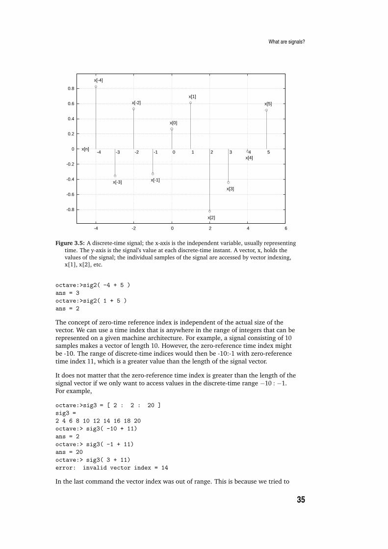
What are signals?
-0.8
-0.6
-0.4
-0.2
0
0.2
0.4
0.6
0.8
-4 -2 0 2 4 6
x[-4]
x[-3]
x[-2]
x[-1]
x[0]
x[1]
x[2]
x[3]
x[4]
x[5]
-4 -3 -2 -1 0 1 2 3 4 5x[n]
Figure 3.5: A discrete-time signal; the x-axis is the independent variable, usually representing
time. The y-axis is the signal’s value at each discrete-time instant. A vector, x, holds the
values of the signal; the individual samples of the signal are accessed by vector indexing,
x[1], x[2], etc.
octave:>sig2( -4 + 5 )
ans = 3
octave:>sig2( 1 + 5 )
ans = 2
The concept of zero-time reference index is independent of the actual size of thevector. We can use a time index that is anywhere in the range of integers that can be
represented on a given machine architecture. For example, a signal consisting of 10samples makes a vector of length 10. However, the zero-reference time index might
be -10. The range of discrete-time indices would then be -10:-1 with zero-reference
time index 11, which is a greater value than the length of the signal vector.
It does not matter that the zero-reference time index is greater than the length of the
signal vector if we only want to access values in the discrete-time range −10 : −1.For example,
octave:>sig3 = [ 2 : 2 : 20 ]
sig3 =
2 4 6 8 10 12 14 16 18 20
octave:> sig3( -10 + 11)
ans = 2
octave:> sig3( -1 + 11)
ans = 20
octave:> sig3( 3 + 11)
error: invalid vector index = 14
In the last command the vector index was out of range. This is because we tried to
35

Creative computing II: interactive multimedia – Volume 1: Creative signals and systems
access the signal using a discrete-time index that was out of range of the signalwhich we determined would represent time indices −10 : −1. Familiarity with
discrete-time indexing and its relationship to vector indexing in Octave will beneeded for working with discrete-time signals and systems.
Learning activity
Construct the following signals in Octave; for each signal, write down the zero-time reference vector index
and use it to access the first and last values of the signal vector using the discrete-time index:
the odd numbers from 23 to 3 with discrete-time index−11 : −1sine function sampled at intervals of π/4 from 0 to 2 ∗ π with discrete-time index 0 : 8
even numbers from 100 to 120 with discrete-time index 10033 : 10053.
3.3.3 The unit impulse
The fundamental building block of discrete-time signal processing is an entity called
the unit impulse. We can think of the unit impulse as being the number 1represented as a signal at discrete-time index 0. The remainder of the signal is zero.
The unit impulse is often called the delta function so it is a signal called δ[n], where
n is the independent variable.
We can construct a function imp in Octave that returns the unit impulse:
octave:1> function result = imp(length,position)
> zeros = zeros(1,length)
> zeros(position)=1
> result = zeros
> endfunction
This user-defined function takes two arguments: the first is the length of the signal
to generate and the second is the position of the 1 within the signal. This position isthe zero-time reference index for the vector. We can now use the function, as shown
below:
octave:>imp(11,6) % Make a unit impulse
zeros =
0 0 0 0 0 0 0 0 0 0 0
zeros =
0 0 0 0 0 1 0 0 0 0 0
result =
0 0 0 0 0 1 0 0 0 0 0
ans =
36
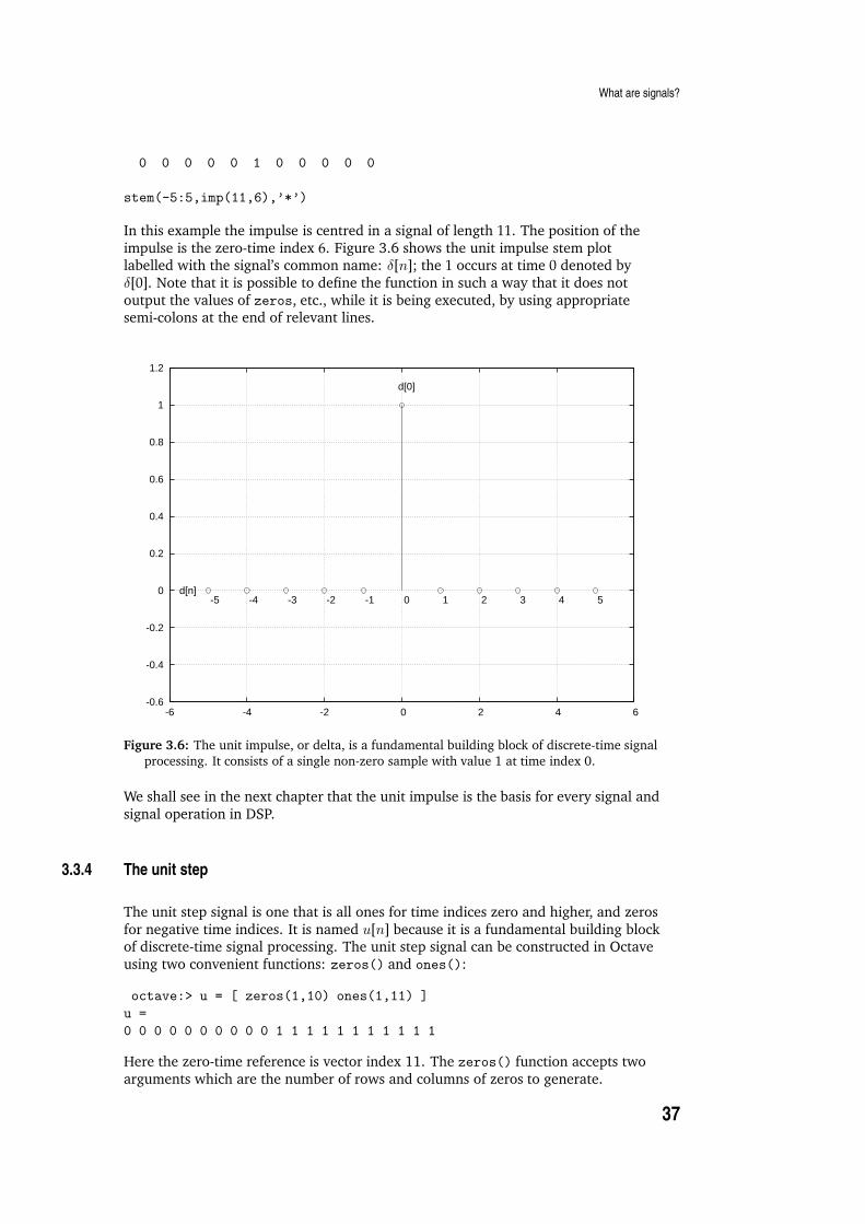
What are signals?
0 0 0 0 0 1 0 0 0 0 0
stem(-5:5,imp(11,6),’*’)
In this example the impulse is centred in a signal of length 11. The position of the
impulse is the zero-time index 6. Figure 3.6 shows the unit impulse stem plotlabelled with the signal’s common name: δ[n]; the 1 occurs at time 0 denoted by
δ[0]. Note that it is possible to define the function in such a way that it does not
output the values of zeros, etc., while it is being executed, by using appropriatesemi-colons at the end of relevant lines.
-0.6
-0.4
-0.2
0
0.2
0.4
0.6
0.8
1
1.2
-6 -4 -2 0 2 4 6
d[0]
-5 -4 -3 -2 -1 0 1 2 3 4 5d[n]
Figure 3.6: The unit impulse, or delta, is a fundamental building block of discrete-time signal
processing. It consists of a single non-zero sample with value 1 at time index 0.
We shall see in the next chapter that the unit impulse is the basis for every signal and
signal operation in DSP.
3.3.4 The unit step
The unit step signal is one that is all ones for time indices zero and higher, and zeros
for negative time indices. It is named u[n] because it is a fundamental building blockof discrete-time signal processing. The unit step signal can be constructed in Octave
using two convenient functions: zeros() and ones():
octave:> u = [ zeros(1,10) ones(1,11) ]
u =
0 0 0 0 0 0 0 0 0 0 1 1 1 1 1 1 1 1 1 1 1
Here the zero-time reference is vector index 11. The zeros() function accepts two
arguments which are the number of rows and columns of zeros to generate.
37
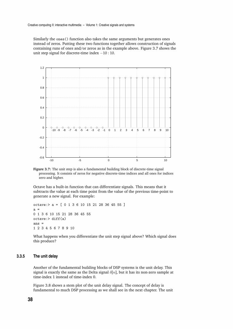
Creative computing II: interactive multimedia – Volume 1: Creative signals and systems
Similarly the ones() function also takes the same arguments but generates onesinstead of zeros. Putting these two functions together allows construction of signals
containing runs of ones and/or zeros as in the example above. Figure 3.7 shows theunit step signal for discrete-time index −10 : 10.
-0.6
-0.4
-0.2
0
0.2
0.4
0.6
0.8
1
1.2
-10 -5 0 5 10
-10 -9 -8 -7 -6 -5 -4 -3 -2 -1 0 1 2 3 4 5 6 7 8 9 10
Figure 3.7: The unit step is also a fundamental building block of discrete-time signal
processing. It consists of zeros for negative discrete-time indices and all ones for indices
zero and higher.
Octave has a built-in function that can differentiate signals. This means that itsubtracts the value at each time point from the value of the previous time-point to
generate a new signal. For example:
octave:> a = [ 0 1 3 6 10 15 21 28 36 45 55 ]
a =
0 1 3 6 10 15 21 28 36 45 55
octave:> diff(a)
ans =
1 2 3 4 5 6 7 8 9 10
What happens when you differentiate the unit step signal above? Which signal doesthis produce?
3.3.5 The unit delay
Another of the fundamental building blocks of DSP systems is the unit delay. This
signal is exactly the same as the Delta signal δ[n], but it has its non-zero sample at
time-index 1 instead of time-index 0.
Figure 3.8 shows a stem plot of the unit delay signal. The concept of delay is
fundamental to much DSP processing as we shall see in the next chapter. The unit
38

What are signals?
delay is the simplest possible representation of the concept of delay. It has the samename as the delta signal, which was notated δ[n], but to represent the delay the time
index is denoted n − 1, so the unit delay is notated as δ[n− 1].
-0.6
-0.4
-0.2
0
0.2
0.4
0.6
0.8
1
1.2
-4 -2 0 2 4 6
d[n-1]
-4 -3 -2 -1 0 1 2 3 4 5 6
Figure 3.8: The unit delay signal is a time-delayed delta signal. The delay is one sample,
which means the time index of the non-zero value is 1 compared with 0 of the delta signal.
The impulse has been delayed by one sample to occur later in time.
This notation indicates that a delay is a subtraction operation that acts on thediscrete-time index of the signal rather than on the signal itself. This process means
that the Delta signal should be looked-up one sample before, −1, the givendiscrete-time index, n. Putting this together, the unit delay is the Delta signal
transformed to a new signal by performing an arithmetic operation on its time
index.
A signal can be delayed by any number of samples using this notation. Consider
Figure 3.9. Here the Delta signal has been delayed by two samples. The notation isnow δ[n − 2] to show that the signal is constructed by looking-up the Delta signal
two samples prior to the given time-index.
Just as we can delay a signal by a given number of samples, we can also advance it
in time. Figure 3.10 shows the Unit Advance signal. This is also constructed out ofthe Delta signal, but the notation is now δ[n+ 1] to indicate that we lookup the Delta
signal one sample ahead of the given time index. A signal may be advanced by any
number of samples; furthermore the relationship between time-advance andtime-delay is now obvious since they are both simply arithmetic operations upon the
time index of a signal. A negative time-delay is equivalent to a time advance; can
you see a mathematical reason why this is so?
39

Creative computing II: interactive multimedia – Volume 1: Creative signals and systems
-0.6
-0.4
-0.2
0
0.2
0.4
0.6
0.8
1
1.2
-4 -2 0 2 4 6
d[n-2]
-4 -3 -2 -1 0 1 2 3 4 5 6
Figure 3.9: The Delta signal delayed by two samples. The notation for delaying the delta
signal, δ[n], by two samples is δ[n − 2] indicating that the Delta signal is to be read at a
given time-index, n, minus two samples. If we do this, the value 1 is produced at
time-index n = 2, because δ[2− 2] = δ[0] = 1 later in time.
-0.6
-0.4
-0.2
0
0.2
0.4
0.6
0.8
1
1.2
-6 -4 -2 0 2 4 6
d[n+1]
-5 -4 -3 -2 -1 0 1 2 3 4 5
Figure 3.10: The unit advance signal is a time-advanced delta signal. The advance is by one
sample, which means the time index of the non-zero value is −1 compared with 0 of the
delta signal. The impulse has been advanced by one sample to occur earlier in time by one
sample.
40
What are signals?
3.3.6 Delay operations in Octave
Delay operations in Octave can be implemented by careful use of the discrete-time
index, the zero-time reference vector index and the time-index arithmeticimplementing delays as discussed above. We must ensure that there is enough space
inside our vector to perform the given delay operation; we do this by padding thesignal at the beginning and end with zeros, making note of the zero-time vector
index reference.
Consider the Delta signal padded with ten zeros on either side of time-index zero
giving zero-time vector reference index 11:
octave:> d = [ zeros(1,10) 1 zeros(1,10) ]
d =
0 0 0 0 0 0 0 0 0 0 1 0 0 0 0 0 0 0 0 0 0
octave:> d( 0 + 11 )
ans = 1
The Delta function can be delayed by one sample, making it a unit delay, by
subtracting one from the discrete-time index:
octave:> d( 0 - 1 + 11 )
ans = 0
octave:> d( 1 - 1 + 11 )
ans = 1
To understand this, we have now used three values for indexing the signal vector.
The first value is the discrete-time index, the second is the amount of delay to
introduce into the signal and the third value is the zero-reference vector index(because Octave uses indices that run from 1 to the length of the signal). We can
perform time advances as either an additive value to the discrete time index, orequivalently, as a negative delay, thus subtracting a negative number from the
discrete-time index.
octave:> d( 0 - -1 + 11 )
ans = 0
octave:> d( 1 - -1 + 11 )
ans = 0
octave:> d( -1 - -1 + 11)
ans = 0
Here the only value of the discrete-time index that outputs the value 1 is time -1.Hence the discrete-time index is advanced by one sample before looking up the
value in the delta signal. Fortunately, Octave provides a more convenient method to
perform time-delays and time-advances on signals than that of using three differentindices. The function is called shift():
octave:> d
d =
0 0 0 0 0 0 0 0 0 0 1 0 0 0 0 0 0 0 0 0 0
octave:> shift(d,1) ans =
0 0 0 0 0 0 0 0 0 0 0 1 0 0 0 0 0 0 0 0 0
octave:> shift(d,-1)
ans =
0 0 0 0 0 0 0 0 0 1 0 0 0 0 0 0 0 0 0 0 0
41
Creative computing II: interactive multimedia – Volume 1: Creative signals and systems
We now have enough knowledge about signals to start to use them to representsound and images for creative computing. The remainder of the Chapter is devoted
to the representation and display of sound and image as signals.
3.4 Audio signals
The ear/brain system interprets certain types of motion in air as sound. The
conditions under which movement in air is heard as sound are complex. When an
object in air undergoes a displacement, the air pressure changes a small amount,near the object, for a short period of time. When a back-and-forth motion is
introduced into the air by an object, called an oscillation, the displacement of air is
also in a back and forth motion causing oscillations in the air pressure.
In general, sounds are caused by objects in the world that vibrate. The vibrationsthat the ear is sensitive to are those that occur between the range of 20 cycles per
second and 20,000 cycles per second. A cycle is a single back-and-forth motion, so
objects that move back and forth more than twenty times per second, but less than20,000 times per second, cause pressure changes in the air that can be heard as
sound.
Air is a gas, so when some of the air molecules are displaced they, in turn, displace
air molecules near them forming a chain reaction in air pressure changes that is
called a pressure wave. The change in air pressure can be detected at a remote pointin space because it is transmitted via the air molecules to that point.
Audio signals represent the displacement of air at a single point in space as
measured by a microphone membrane. Displacement of the membrane generates an
electrical signal that is proportional to the displacement. The process of digitalsampling is that of recording the level of the electrical signal at fixed time intervals
called the sampling period. The measured value is recorded in digital memory as
either an integer or a floating point number for each sample.
To play back an audio signal the digitally sampled signal must first be converted
back to an analogue electrical signal and then this signal used to displace the cone,or membrane, in a loudspeaker or headphones. The operation of moving the air
using a loudspeaker generates movement in air that is similar to the movement thatwe measured with a microphone.
Again, reference to a relevant textbook will be helpful for you, as these are standardaudio signal processing concepts.
3.4.1 Sampling
As mentioned above, sampling is the process of measuring the value of somephenomenon at regular intervals, called the sampling period. If measured in
seconds, the sampling period is inversely proportional to the sampling frequency,
also called the sample rate: SR. To capture the variation in the measured value of aphenomenon, such as sound, we must know in advance what the maximum
frequency will be. Then we make sure that we measure the source often enough to
capture the variation at this maximum frequency.
The maximum frequency that is audible by humans is in the region of 20kHz. So we
42
Audio signals
must be able to capture variation in a signal that is close to 20kHz. To do this wemust use a sampling rate that is at least twice the maximum frequency that we want
to measure. This is because the maximum frequency that can be detected bysampling is half the sample rate: SR/2. This latter frequency is called the Nyquistfrequency named after the engineer Harry Nyquist who first recognised its
importance. If we make the Nyquist frequency the maximum frequency we want todetect, such as 20kHz in the case of audio, then the sampling rate will be double this
maximum frequency: 40kHz.
The most commonly used sample rate used for digital audio is 44.1kHz which is just
slightly above that required for detecting frequencies at 20kHz. Other common
sample rates are 22.05kHz, 11.025kHz, 96kHz, 48kHz, 32kHz, 16kHz and 8kHz. Whatare the Nyquist frequencies for each of these sampling rates?
Learning activity
Show why if you do not sample at twice the frequency, you can lose vital information about the wave.
Digital audio
Digital audio is the application of discrete-time signal construction and signal
processing to applications using sound. As such, the sine and cosine functions, sin()
and cos(), are often used as sound atoms; they are the building blocks of digitalaudio.
The definition of the sine and cosine functions comes from the coordinates of theunit circle. At each point on the unit circle, the angle of the line from the origin to
that point has the cosine value of the point’s x-coordinate and the sine value of the
point’s y-coordinate.
Figure 3.11 illustrates the relationship between angle, a point on the unit circle and
the sin() and cos() functions. To construct a sine wave in time, we consider apoint starting at a given angle on the unit circle, and imagine it travelling at a
constant speed around the circumference of the unit circle. At each moment in time,the height of the point above or below the x-axis makes the sine wave through time.
Audio occurs in time and is due to oscillation in air. A fundamental form ofoscillation is a sine wave; which is the sin() function through time. When played as
a sound a sine wave is heard as a pure tone, such as the sustained part of a tuning
fork sound.
3.4.2 Frequency
The frequency of a sine wave is the number of oscillations, or cycles, per second.
That is, the number of complete revolutions around the unit circle tracing out theheight of a point travelling on its circumference. The faster the point travels around
the unit circle, the higher the frequency.
From elementary mathematics, the circumference of a circle is 2πr with r the radius.
The unit circle has radius 1 so the circumference has length 2π. For a given point on
43
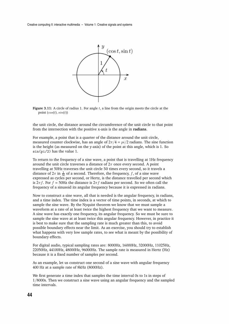
Creative computing II: interactive multimedia – Volume 1: Creative signals and systems
Figure 3.11: A circle of radius 1. For angle t, a line from the origin meets the circle at the
point (cos(t), sin(t))
the unit circle, the distance around the circumference of the unit circle to that pointfrom the intersection with the positive x-axis is the angle in radians.
For example, a point that is a quarter of the distance around the unit circle,measured counter clockwise, has an angle of 2π/4 = pi/2 radians. The sine function
is the height (as measured on the y-axis) of the point at this angle, which is 1. Sosin(pi/2) has the value 1.
To return to the frequency of a sine wave, a point that is travelling at 1Hz frequencyaround the unit circle traverses a distance of 2π once every second. A point
travelling at 50Hz traverses the unit circle 50 times every second, so it travels a
distance of 2π in 150
of a second. Therefore, the frequency, f , of a sine waveexpressed as cycles per second, or Hertz, is the distance travelled per second which
is 2πf . For f = 50Hz the distance is 2πf radians per second. So we often call the
frequency of a sinusoid its angular frequency because it is expressed in radians.
Now to construct a sine wave, all that is needed is the angular frequency, in radians,and a time index. The time index is a vector of time points, in seconds, at which to
sample the sine wave. By the Nyquist theorem we know that we must sample a
waveform at a rate of at least twice the highest frequency that we want to measure.A sine wave has exactly one frequency, its angular frequency. So we must be sure to
sample the sine wave at at least twice this angular frequency. However, in practice it
is best to make sure that the sampling rate is much greater than this, to avoidpossible boundary effects near the limit. As an exercise, you should try to establish
what happens with very low sample rates, to see what is meant by the possibility of
boundary effects.
For digital audio, typical sampling rates are: 8000Hz, 16000Hz, 32000Hz, 11025Hz,22050Hz, 44100Hz, 48000Hz, 96000Hz. The sample rate is measured in Hertz (Hz)
because it is a fixed number of samples per second.
As an example, let us construct one second of a sine wave with angular frequency
400 Hz at a sample rate of 8kHz (8000Hz).
We first generate a time index that samples the time interval 0s to 1s in steps of
1/8000s. Then we construct a sine wave using an angular frequency and the sampled
time intervals.
44

Audio signals
octave:>t = [ 0 : 1/8000 : 1 ] ;
octave:> x = sin( 2 * pi * 400 * t) ;
octave:>stem(t(1:20), x(1:20),’*’)
Note that this example uses a semicolon at the end of each line that generates a
vector. A semicolon in Octave is used as a command separator, but it has anotherfunction, that is to suppress the printing of results of operations to the terminal. The
vectors for audio signals are very long – in this case 8001 samples – so we want to
suppress Octave’s default behaviour of printing vectors to the screen. When you havemade your plot of the sine wave you should see a figure like that of Figure 3.12.
We computed 8001 values for one second of the sine wave. The extra sample isbecause we sampled up to and including the 1s boundary, which made the example
easier to read. To generate exactly 8,000 samples, i.e. exactly one second of audio,we should use: t = [0 : 1/8000 : 1 - 1/8000] or, equivalently, t = [0 :
7999] / 8000.
-1
-0.5
0
0.5
1
0 0.0005 0.001 0.0015 0.002 0.0025
Am
plitu
de
Time (s)
Figure 3.12: One complete cycle of a A 400Hz sine wave sampled with a sampling rate of
8000Hz (8kHz). The time index is in seconds.
The example above plotted only 20 samples of the signal instead of the entire signal.
This is for two reasons: the first is that 8,000 samples is a lot of data, and plotting itwould produce an unreadable graph. Secondly, this number of samples was chosen
to plot because it is exactly one complete cycle out of the 400 cycles in the onesecond signal that we generated.
Plotting an audio signal is useful to check that we have performed the correctoperations. We see an oscillating waveform that has a maximum height of 1, and
that the duration is 0.0025 seconds, which is 1/400s; that is, the amount of time that
a single cycle of a 400Hz signal occupies. But plotting the signal is not the same ashearing it, so let us listen to the entire signal.
We can play digital audio in Octave using the sound() function. Sound takes two
45
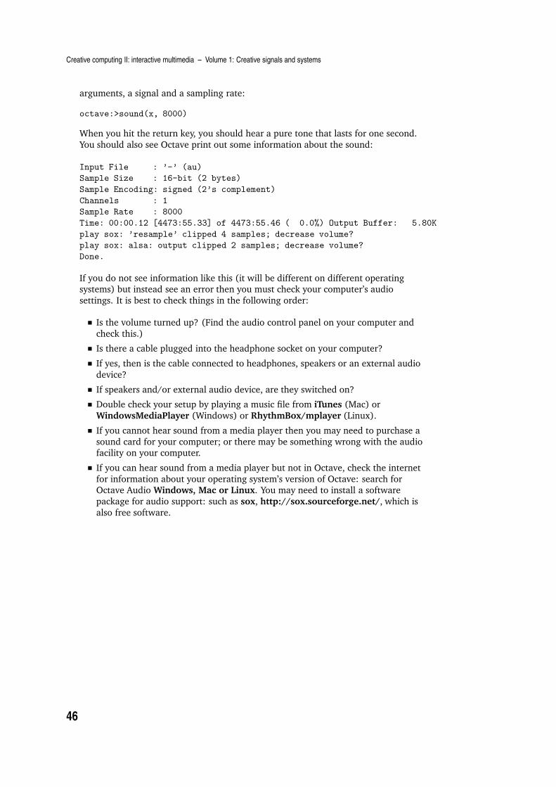
Creative computing II: interactive multimedia – Volume 1: Creative signals and systems
arguments, a signal and a sampling rate:
octave:>sound(x, 8000)
When you hit the return key, you should hear a pure tone that lasts for one second.
You should also see Octave print out some information about the sound:
Input File : ’-’ (au)
Sample Size : 16-bit (2 bytes)
Sample Encoding: signed (2’s complement)
Channels : 1
Sample Rate : 8000
Time: 00:00.12 [4473:55.33] of 4473:55.46 ( 0.0%) Output Buffer: 5.80K
play sox: ’resample’ clipped 4 samples; decrease volume?
play sox: alsa: output clipped 2 samples; decrease volume?
Done.
If you do not see information like this (it will be different on different operatingsystems) but instead see an error then you must check your computer’s audio
settings. It is best to check things in the following order:
Is the volume turned up? (Find the audio control panel on your computer and
check this.)
Is there a cable plugged into the headphone socket on your computer?
If yes, then is the cable connected to headphones, speakers or an external audio
device?
If speakers and/or external audio device, are they switched on?
Double check your setup by playing a music file from iTunes (Mac) or
WindowsMediaPlayer (Windows) or RhythmBox/mplayer (Linux).
If you cannot hear sound from a media player then you may need to purchase a
sound card for your computer; or there may be something wrong with the audiofacility on your computer.
If you can hear sound from a media player but not in Octave, check the internet
for information about your operating system’s version of Octave: search forOctave Audio Windows, Mac or Linux. You may need to install a software
package for audio support: such as sox, http://sox.sourceforge.net/, which is
also free software.
46
Audio signals
Learning activity
Make the following sine waves and play them using the sound() command in Octave: (Note: If you
cannot get the sound command to work in Octave, but your media player works, then you can save your
sound using the wavwrite() command and then open it in your media player to hear it.)
a 1s 1000Hz sine wave at 8000Hz sample rate
a 1s 50Hz sine wave at 8000Hz sample rate
a 1s 8000Hz sine wave at 32000Hz sample rate
a 1s 11000Hz since wave at 44100Hz sample rate.
For each of the sine waves above:
make a stem plot of one cycle of the sine wave: (the number of samples in one cycle is SR/f where
SR is the sample rate and f is the angular frequency of the sine wave)
play the sound of one cycle of the sine wave (instead of one second): what do you hear?
play the sound of five cycles of the sine wave (instead of one second): what do you hear?
play the sound of twenty cycles of the sine wave (instead of one second): what do you hear?
3.4.3 Amplitude
The maximum height of the waveform is its amplitude or peak amplitude. In
Octave, sounds are represented by floating-point numbers in the range −1.0 to 1.0;any sound that has a greater range than this is scaled so that it fits within this range.
The sine waves we generated above have amplitude 1; so they are at the maximum
range for sound in Octave.
The perceived intensity of the sound is relative to its amplitude. To change the
perceived intensity of a sound the waveform is divided (or multiplied) by a scalar.For example, dividing the sound by 10 will result in an amplitude that is 10 times
smaller. However, the sound that is heard will be perceived as approximately half as
loud. This is due to the way the ear responds non-linearly to changes in a sound’samplitude.
A common measure of a sound’s level, or loudness, is decibels (dB). Decibels can be
computed from a sine wave’s amplitude using the following expression:
decibels = 20 * log10( max(sig)) )
For a sine wave at full volume the loudness – relative to the gain in the speakers – isat 0dB. This is called the reference; all other loudness levels are measured with
respect to this reference loudness.
We might be able to amplify the output of Octave using speakers so that the loudness
is perceived to be the same as normal conversation. Given this loudness reference,
Table 3.1 is a guide for relative loudness of different sounds at different decibellevels:
47

Creative computing II: interactive multimedia – Volume 1: Creative signals and systems
dB Amplitude factor Sound Perceived loudness
-0 1 Normal conversation 1
-10 0.3162 Quiet suburban outdoors 1/2-20 0.1 Buzz of mosquito 1/4-30 0.03162 Watch ticking 1/8-40 0.01 Quiet house interior 1/16-50 0.003162 Rustling leaves 1/32-60 0.001 Threshold of hearing (silence) 1/64
Table 3.1: Table of relative loudness levels for sounds across the entire range of human
hearing.
A change of -10dB represents half the perceived loudness; and a change of −20dB isa change of half of a half which is a quarter of the loudness. Therefore each loudness
step in Table 3.1 is a perceived change of a factor of two in loudness.
To change the loudness of a sine wave we multiply the signal by a scalar. To do this,
first turn the speakers up to the reference loudness of 0dB and then attenuate the
signal by multiplication with a scalar < 1.0 to the desired loudness level relative tothe 0dB reference.
octave:>sound( x, 8000 ) % reference level of 0dB
octave:>sound( 0.31623 * x, 8000 ) % -10dB = half the loudness of 0dB
octave:>sound( 0.1 * x, 8000 ) % -20dB = quarter of the loudness of
0dB
octave:>sound( 0.031623 * x, 8000 ) % -30dB = eight of the loudness of
0dB
octave:>sound( 0.01 * x, 8000 ) % -40dB = sixteenth of the loudness of
0dB
As well as sine waves, we can generate noise very easily in Octave. Noise is simply
uniform randomness which in Octave is generated by the rand() function. Thisfunction takes two arguments: the number of rows and columns of the vector that it
generates. It generates uniform random real numbers in the range 0 to 1; to make
them occupy the full audio range we multiply the output of the rand() function by 2and subtract 1. Now the random numbers will be in the range −1 to 1 as in the
following example.
octave:>x = rand(1,8000)*2-1;
octave:>sound(x,8000);
When you play this example you should hear a loud noise that lasts for one second.
Noise is another fundamental unit for constructing audio signals and it is very often
used to make synthetic percussion sounds such as snare drums, cymbals and otherinstruments. Noise has a very interesting property with regard to its frequency
content. Recall that a sine wave has exactly one frequency present, while noise hasall frequencies present in the signal (at random amplitudes). This remarkable fact
makes uniform random noise a very useful signal. Figure 3.13 shows a stem plot of a
randomly-generated signal.
48

Audio signals
-1
-0.8
-0.6
-0.4
-0.2
0
0.2
0.4
0.6
0.8
1
0 0.0005 0.001 0.0015 0.002 0.0025
Am
plitu
de
Time (s)
Figure 3.13: Twenty samples of a random signal sampled at 8000Hz. It is not possible to
select a single cycle of a random signal because all frequencies are present. The signal is
generated in the range −1 to 1 so it has a peak amplitude of 1.
Learning activity
Using the noise signal, x, generated above, play back the sound at the following different loudness levels:
−10dB−20dB−30dB−40dB−50dB−60dB.
At what level can you no longer hear the sound?
3.4.4 Phase
Other than amplitude, angular frequency and a time index, there is another
parameter available for sine waves; that is the phase offset. A phase offset occurswhen the sine wave starts at an angle (in radians) other than 0. Figure 3.14 shows a
sine wave with the same frequency and amplitude as Figure 3.12 but that starts, at
time 0, with a phase offset of pi/8 radians.
49

Creative computing II: interactive multimedia – Volume 1: Creative signals and systems
Instead of starting with a height of 0 at time 0, this sine wave starts with a value of0.38268 at time 0. This corresponds to the value of a sine wave at pi/8 radians. The
remaining values continue the sine function for the given angular frequency but theyare all offset by pi/8 radians.
To implement a phase offset in Octave we add the phase offset to the instantaneousphase argument of the sin() function:
octave:>x = sin( 2 * pi * 400 * t + pi/8);
octave:>stem(t(1:20),x(1:20))
-1
-0.8
-0.6
-0.4
-0.2
0
0.2
0.4
0.6
0.8
1
0 0.0005 0.001 0.0015 0.002 0.0025
Am
plitu
de
Time (s)
Figure 3.14: One complete cycle of a 400Hz sine wave with phase offset of pi/8.
We can offset a sine wave by any angle. For example, let’s see what happens when
we offset the sine wave by an angle of pi/2 radians:
octave:>x = sin( 2 * pi * 400 * t + pi/2);
octave:>stem(t(1:20),x(1:20))
One cycle of the resulting signal is shown in Figure 3.15. What is the value of this
signal at time 0? Contrast this with the value of the signal with phase offset of 0.Which mathematical function has been generated by a sine wave with a phase offset
of pi/2?
Additive synthesis
A sinusoid is a sine wave that can have any amplitude, frequency and phase offset;
i.e. sin() and cos() are both sinusoids; they are instances of the same curve butthey are offset by pi/2. It is a remarkable fact about sinusoids that a number of
them can be summed to make any signal. There must be the correct number with
correct amplitudes, frequencies and phase offsets, but it is a fact that they can be
50

Audio signals
-1
-0.5
0
0.5
1
0 0.0005 0.001 0.0015 0.002 0.0025
Am
plitu
de
Time (s)
Figure 3.15: One complete cycle of a 400Hz sine wave with phase offset of π/8.
51

Creative computing II: interactive multimedia – Volume 1: Creative signals and systems
seen as the fundamental elements of all signals. Therefore, sinusoids form a basisover signals; they are the sound atoms from which signals can be constructed.
To see how sinusoids can be used to make complex waveforms we consider thesimple case of adding sinusoids with different amplitudes and frequencies. First, let
us add two sinusoids, where the second has double the frequency of the first:
octave:> x1 = sin( 2 * pi * 400 * t);
octave:> x2 = sin( 2 * pi * 800 * t);
octave:>complexSig = ( x1 + x2 ) / 2;
octave:>sound( complexSig * 0.3162, 8000)
octave:>stem( t(1:20), complexSig(1:20) )
Figures 3.16 to 3.18 show successive plots of the signals after adding one more
sinusoid to the signal obtained from the previous one. Work through all of theseexamples successively. How do the sounds compare with previous and subsequent
tones?
-1
-0.8
-0.6
-0.4
-0.2
0
0.2
0.4
0.6
0.8
1
0 0.0005 0.001 0.0015 0.002 0.0025
Am
plitu
de
Time (s)
Figure 3.16: One complete cycle of a complex signal formed by summing two sinusoids with
frequencies 400Hz and 800Hz. The amplitudes of the sinusoids were halved after summing
so that the amplitude remained at 1.
52

Audio signals
-1
-0.8
-0.6
-0.4
-0.2
0
0.2
0.4
0.6
0.8
1
0 0.0005 0.001 0.0015 0.002 0.0025
Am
plitu
de
Time (s)
Figure 3.17: One cycle of a complex signal formed by summing three sinusoids with
frequencies 400Hz, 800Hz and 1200Hz. The amplitudes were divided by 3 giving a peak
amplitude of 1 in the resulting complex signal.
53

Creative computing II: interactive multimedia – Volume 1: Creative signals and systems
-0.8
-0.6
-0.4
-0.2
0
0.2
0.4
0.6
0.8
0 0.0005 0.001 0.0015 0.002 0.0025
Am
plitu
de
Time (s)
Figure 3.18: One cycle of a complex signal formed by summing four sinusoids with
frequencies 400Hz, 800Hz, 1200Hz and 1600Hz. The amplitudes were divided by 4 giving a
peak amplitude of 1 in the resulting complex signal.
54

Exercises
3.5 Summary and learning outcomes
This chapter provides an introduction to basic signal processing, through the use of
the Octave software. It introduced some important signals, namely the unit impulse,the unit step, and the unit delay. It then went on to discuss sampling of audio
signals, and described how changes in frequency, amplitude and phase affect sounds.
With a knowledge of the contents of this chapter and its directed reading and
activities, you should be able to:
use Octave to perform basic signal processing tasks, as well as generate plots ofsignals
describe what a signal is, and in particular what a one-dimensional signal is
discuss the significance of the unit impulse, the unit step, and the unit delay in
signal processing
perform various delay operations using Octave
discuss what the Nyquist frequency is, and how it relates to sound and digital
processing
describe frequency, amplitude and phase as properties of signals.
3.6 Exercises
1. Type the following lines into Octave. This code makes a vector of sinusoid
samples x, plots one cycle of the sinusoid and plays the sinusoid as audio at asample rate of 11.025kHz. This sample rate is the default setting for Octave. You
can use the command setaudio to change the sample rate in Octave.
amp = 0.3162; % sinusoid amplitude (-10dB)
freq = 110; % frequency in Hertz (cps)
dur = 2.0; % duration in seconds
sr = 16000; % the audio sample rate
phase= 0; % initial phase (phase offset)
n = [ 0 : dur * sr ]; % sample index vector
x = sin( 2 * pi * freq / sr * n + phase ); % The sinusoid generator
plot( [ 0 : ceil(sr/freq) - 1 ] / sr , x( 1 : ceil(sr/freq) )) % Plot one
%cycle grid add grid markings to the plot
sound( x, 16000 ) % play the sound
Experiment with the interactive command-line by making sinusoids of 220Hz,
440Hz and 130.81Hz, 261.63Hz and 523.25Hz; these correspond to the musical
pitches A3, A4 and C2, C3 and C4. Play the audio for these sinusoids; can youhear the musical scale relationships?
(a) Plot your sinusoids on the same graph by typing hold on in Octave.
(b) Choose a melody and construct it out of a set of sinusoids by playing themone after the other. The melody could be a favourite song, or your national
anthem, for example.
2. The interactive command line is useful but a bit slow. To speed up making
sinusoids we can make a function. Use a text editor to type in the followingfunction and save it as an Octave function in a file called sinusoid.m.
55

Creative computing II: interactive multimedia – Volume 1: Creative signals and systems
function [y, n] = sinusoid(A, f, dur, sr, phi)
% y = sinusoid(A, f, d, sr, phi)
%
% A - amplitude
% f - frequency in Hertz
% d - duration in seconds (1.0)
% sr - sample rate in Hertz (44100)
% phi - initial phase n Radians (0)
if nargin<5, phi=0; end % default phase
if nargin<4, sr=16000; end % default sr
if nargin<3, dur=1; end % default dur
if nargin<2, f=440; end % default freq
if nargin<1, A=0.3162;end % default amplitude (-10dB)
n = [0:ceil(dur*sr)-1]./sr; % sample index
y = A * sin ( 2*pi*f*n + phi ); % sinusoid
p = sum(y.^2) / length(n); % average power
To use the function you will need to typeaddpath(’/Volumes/myDisk/myPath/’). This function returns a vector of
sinusoid samples as its first return argument, and a vector of time instants as its
second return argument. For example:
octave:>[x,t] = sinusoid(100, 440, 2, 11025, pi/2);
octave:>stem(t(1:20),x(1:20),’*’)
(a) Using your newly created function, plot sinusoids of the following
frequencies:
110Hz
220Hz
330Hz
440Hz.
3. So far we have made simple tones. Helmholtz studied the composition of
complex tones. We make complex tones by summing simple tones (sinusoids) ofdifferent amplitudes, frequencies and phases.
We can efficiently compute the partials for a harmonic series using a for loop in
Octave.
amp = 0.3162; % amplitude
freq = 220; % frequency
dur = 2; % duration
phase = 0; % phase
sr = 44100; % sample rate
N=10; % Number of partials
x = zeros( 1, ceil(dur*sr)); % initial empty vector
for k=1:N
x = x + (1/N)*sinusoid( amp, k * freq, dur, sr, phase);
end
stem([0:length(x(1:ceil(sr/freq)))]/sr,*x(1:ceil(sr/freq)) % Automatically plot one cycle
sound(x*.01) % scale audio by number of partials
If Octave does not graph your function then the graphics may need re-setting.
Use the command close all to close all open graphics windows and reset the
axis scaling.
56

Exercises
(a) Use a for-loop, similar to the example above, to construct each of thefollowing waveforms with a sample rate of 44.1kHz:
ten harmonics with amplitude (1− k/10) ∗ amp
ten harmonics with amplitude k/10
ten harmonics with amplitude exp(0.5 ∗ −k) ∗ amp
ten harmonics with amplitude exp(0.5 ∗ k) ∗ amp
the fundamental and even harmonics up to ten harmonics [ 1 2 4 6 8 10 ]
the fundamental and odd harmonics up to ten harmonics [ 1 3 5 7 9 ].
(b) Listen to each of your waveforms. Describe the sounds that you hear.
4. Using the sinusoid function from above, make two sinusoid vectors called x and
y, each with amplitude 0.3162 and frequency 220 Hertz, but x should have aphase offset of 0 and y should have a phase offset of π (pi in Octave and PI in
MATLAB).
(a) What is the difference between these waveforms? Is there an easy way to
derive y from x and vice-versa?
(b) Now make the following waveforms:
ten harmonics with amplitude (1− k/10) ∗ amp with alternating phases
0, pi
ten harmonics with amplitude exp(0.5 ∗ −k) ∗ amp with alternatingphases 0, pi
the fundamental and odd harmonics up to ten harmonics [ 1 3 5 7 9 ]with alternating phases 0, pi.
(c) Plot these waveforms against the corresponding waveforms from above.
What is the difference?
(d) Now listen to each of these waveforms against the corresponding waveforms
from above. What is the difference between the two?
5. Make a cosine wave using a sine wave with a phase offset of π2(pi/2). Play
both of the signals using the sound() function. Is there an audible differencebetween the sine wave and cosine wave? Explain your answer.
57

Creative computing II: interactive multimedia – Volume 1: Creative signals and systems
58

Chapter 4
Systems
Essential reading
Eaton, J.W. GNU Octave Manual. (Bristol: Network Theory, 1996) [ISBN 0954161726]. (This is also
available online in HTML form at
http://www.gnu.org/software/octave/doc/interpreter and in texinfo source format in
the Octave source code distribution.)
Recommended reading
Oppenheim, A.V. and A.S. Willsky with S. Hamid Nawab Signals and Systems. (Upper Saddle River, N.J.; London:
Prentice Hall, 1997) [ISBN 0138147574].
4.1 Introduction
The previous chapter discussed how increasingly complex signals can be constructed
by summing fundamental signal building blocks called sinusoids. Digital signalprocessing is concerned with both the construction and transformation of signals to
make new signals. The transformation processes are made from combinations of
fundamental transformation building blocks; collectively, these transformations arecalled systems.
A system responds to an input signal to produce a new output signal. Examples ofinput signals and system responses include:
the electromagnetic spectrum and the radio
the hammer and the church bell
the electric current and the dimmer switch
the bow on the string and the violin body
the bump on the road and the car’s suspension
the bat’s chirp and the echo from an insect
the lightning strike and the rolling thunder
the glottis and the vocal tract (speech)
the baseball on the bat and the ‘pop’
the penny dropped and the resulting ring.
In all of these examples an initial signal is transformed into another signal via a
system. The system can be simple, as in the case of the dimmer switch which is avariable resistor, or very complex as in the case of rolling thunder (which is due to
the acoustic properties of air and the geography and architecture of the region of the
lightning strike).
59
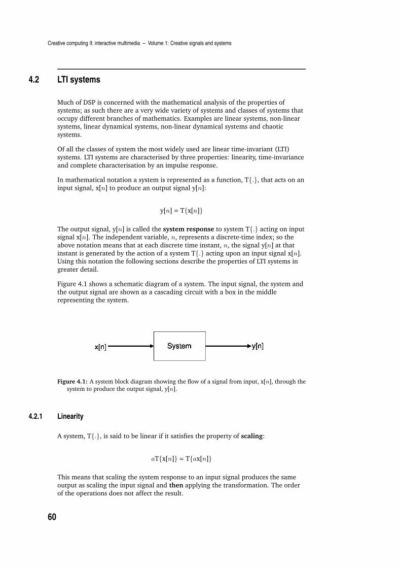
Creative computing II: interactive multimedia – Volume 1: Creative signals and systems
4.2 LTI systems
Much of DSP is concerned with the mathematical analysis of the properties ofsystems; as such there are a very wide variety of systems and classes of systems that
occupy different branches of mathematics. Examples are linear systems, non-linearsystems, linear dynamical systems, non-linear dynamical systems and chaotic
systems.
Of all the classes of system the most widely used are linear time-invariant (LTI)
systems. LTI systems are characterised by three properties: linearity, time-invariance
and complete characterisation by an impulse response.
In mathematical notation a system is represented as a function, T{.}, that acts on an
input signal, x[n] to produce an output signal y[n]:
y[n] = T{x[n]}
The output signal, y[n] is called the system response to system T{.} acting on inputsignal x[n]. The independent variable, n, represents a discrete-time index; so the
above notation means that at each discrete time instant, n, the signal y[n] at that
instant is generated by the action of a system T{.} acting upon an input signal x[n].Using this notation the following sections describe the properties of LTI systems in
greater detail.
Figure 4.1 shows a schematic diagram of a system. The input signal, the system and
the output signal are shown as a cascading circuit with a box in the middlerepresenting the system.
Figure 4.1: A system block diagram showing the flow of a signal from input, x[n], through the
system to produce the output signal, y[n].
4.2.1 Linearity
A system, T{.}, is said to be linear if it satisfies the property of scaling:
aT{x[n]} = T{ax[n]}
This means that scaling the system response to an input signal produces the same
output as scaling the input signal and then applying the transformation. The orderof the operations does not affect the result.
60

LTI systems
Linear systems also obey the property of superposition for sums of signals:
aT{x[n]} + bT{y[n]} = T{ax[n] + by[n]}
This property demonstrates one of the main utilities of linear systems; there are twotransformations on the left-hand side of the equation and only one transformation
on the right-hand side. Linear systems allow algebraic manipulation of signals and
systems to find a more efficient way to implement the transformations. Thisprincipal is very important to the field of digital signal processing because, often, the
goal is to perform complex tasks with limited computational means.
4.2.2 Time invariance
The property of time invariance means that a system responds in the same manner
to its input at all instants in time. So there is no dependence on the variable n in theaction of the system.
Formally, this concept is notated by:
y[n] = T{x[n + d]} → y[n − d] = T{x[n]}∀n
4.2.3 Impulse response
LTI systems are completely characterised by their impulse response. The impulse
response is the system response given the delta function (the impulse) as input.
By convention, we call the impulse signal d[n] and the impulse response of a system
h[n]. Figure 4.2 shows the system block diagram of an impulse response.
Figure 4.2: The impulse response of a system is the system response to the delta signal input.
The delta signal is called the unit impulse. The impulse response completely characterises
an LTI system.
The fact that an impulse reponse characterises an LTI system means that once we
know the impulse response of a system, we know exactly how the system will
respond to any signal. The impulse response is a precise description of an LTIsystem.
This fact means that we can implement an LTI system by transforming a signal withthe impulse response of a system. The operation that transforms a signal using an
61
Creative computing II: interactive multimedia – Volume 1: Creative signals and systems
impulse response is called convolution.
The impulse response is itself a discrete-time signal. This means that systems are
implemented by convolving two signals. We will now discuss the convolutionoperator in more detail.
4.2.4 Convolution
Convolution is represented by a special operator notated as ∗. This is not to be
confused with the multiplication operator that uses the same symbol in most
computer programming languages:
y[n] = x[n] ∗ h[n]
The convolution operator implements the convolution sum, which is a widely-usedoperation in mathematics:
y[n] =
∞∑
k=−∞
h[k]x[n − k]
This notation informs us that the output at each time instant, n, is formed by addingthe impulse response, h[n] to the current output time location, y[n] and scaling it by
the current input value x[n].
In Octave, the convolution operator is provided by a function call, conv(). The
following example shows the use of the convolution operator to transform a uniformrandom signal, with length 10, using an impulse response of length 2:
octave:>x = rand(1,10); % A random signal of length 10
octave:>h = [0.5 0.5]; % An impulse response
octave:>y = conv(x, h);% Convolution operation
octave:>subplot(211)
octave:>stem(0:length(x)-1, x,’*’)
octave:>axis([-1 length(y) 0 1])
octave:>subplot(212)
octave:>stem(0:length(y)-1,y,’*’)
octave:>axis([-1 length(y) 0 1])
The length of the input signal x is 10 and the impulse response h has length 2 in this
case. The convolution operation produces a signal that is length(x) + length(h)
- 1, so the length of the output signal y is therefore 11.
The signal in Figure 4.3 is transformed to that of Figure 4.4 via the system withimpulse response h = [0.5 0.5]. We often call the process of convolving a signal
with an impulse response filtering, because it helps us to extract specific parts of asignal. In this case the system is a two-point averaging filter. As we shall see in the
following chapter, this corresponds to a low-pass filter which means that high
frequencies present in the signal are attenuated and low frequencies are passedthrough unchanged.
62

LTI systems
0
0.2
0.4
0.6
0.8
1
0 2 4 6 8 10
Figure 4.3: A signal of length 10 generated using Octave’s rand() function.
0
0.2
0.4
0.6
0.8
1
0 2 4 6 8 10
Figure 4.4: The signal of Figure 4.3 convolved with the two-point impulse response [0.5
0.5]. The convolved signal has length length(x)+length(h)-1 which is 11 samples.
63
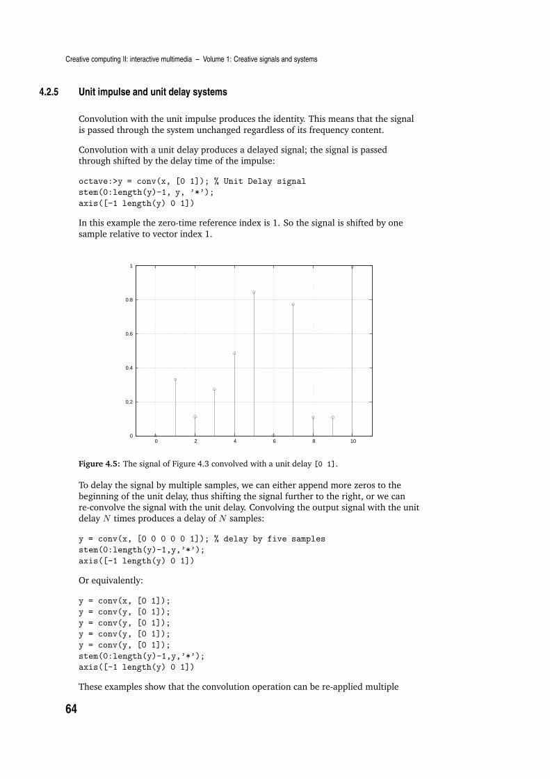
Creative computing II: interactive multimedia – Volume 1: Creative signals and systems
4.2.5 Unit impulse and unit delay systems
Convolution with the unit impulse produces the identity. This means that the signal
is passed through the system unchanged regardless of its frequency content.
Convolution with a unit delay produces a delayed signal; the signal is passedthrough shifted by the delay time of the impulse:
octave:>y = conv(x, [0 1]); % Unit Delay signal
stem(0:length(y)-1, y, ’*’);
axis([-1 length(y) 0 1])
In this example the zero-time reference index is 1. So the signal is shifted by one
sample relative to vector index 1.
0
0.2
0.4
0.6
0.8
1
0 2 4 6 8 10
Figure 4.5: The signal of Figure 4.3 convolved with a unit delay [0 1].
To delay the signal by multiple samples, we can either append more zeros to the
beginning of the unit delay, thus shifting the signal further to the right, or we can
re-convolve the signal with the unit delay. Convolving the output signal with the unitdelay N times produces a delay of N samples:
y = conv(x, [0 0 0 0 0 1]); % delay by five samples
stem(0:length(y)-1,y,’*’);
axis([-1 length(y) 0 1])
Or equivalently:
y = conv(x, [0 1]);
y = conv(y, [0 1]);
y = conv(y, [0 1]);
y = conv(y, [0 1]);
y = conv(y, [0 1]);
stem(0:length(y)-1,y,’*’);
axis([-1 length(y) 0 1])
These examples show that the convolution operation can be re-applied multiple
64
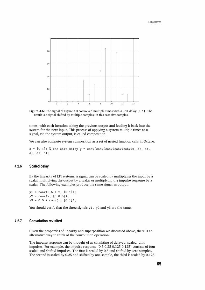
LTI systems
0
0.2
0.4
0.6
0.8
1
0 2 4 6 8 10 12 14
Figure 4.6: The signal of Figure 4.3 convolved multiple times with a unit delay [0 1]. The
result is a signal shifted by multiple samples; in this case five samples.
times; with each iteration taking the previous output and feeding it back into the
system for the next input. This process of applying a system multiple times to asignal, via the system output, is called composition.
We can also compute system composition as a set of nested function calls in Octave:
d = [0 1]; % The unit delay y = conv(conv(conv(conv(conv(x, d), d),
d), d), d);
4.2.6 Scaled delay
By the linearity of LTI systems, a signal can be scaled by multiplying the input by a
scalar, multiplying the output by a scalar or multiplying the impulse response by ascalar. The following examples produce the same signal as output:
y1 = conv(0.5 * x, [0 1]);
y2 = conv(x, [0 0.5]);
y3 = 0.5 * conv(x, [0 1]);
You should verify that the three signals y1, y2 and y3 are the same.
4.2.7 Convolution revisited
Given the properties of linearity and superposition we discussed above, there is analternative way to think of the convolution operation.
The impulse response can be thought of as consisting of delayed, scaled, unit
impulses. For example, the impulse response [0.5 0.25 0.125 0.125] consists of four
scaled and shifted impulses. The first is scaled by 0.5 and shifted by zero samples.The second is scaled by 0.25 and shifted by one sample, the third is scaled by 0.125
65

Creative computing II: interactive multimedia – Volume 1: Creative signals and systems
and shifted by two samples, and the fourth is also scaled by 0.125 but shifted bythree samples.
By the property of superposition, convolution can be calculated as shifting andscaling the input signal by each scaled and shifted impulse in the impulse response
and summing the four system responses:
y = conv(x, [0.5 0 0 0]);
y = y + conv(x, [0 0.25 0 0]);
y = y + conv(x, [0 0 0.125 0]);
y = y + conv(x, [0 0 0 0.125]);
You should verify that the output of this set of operations is the same as convolution
of the input signal with the impulse response [0.5 0.25 0.125 0.125].
This example illustrates a very important property of convolution, namely that the
operation can be broken into a number of very simple steps:
delay the signal
scale the signal
sum it with the output signal.
It was stated above that the output of the convolution operation is a signal that has
length length(x) + length(h) -1. For an input signal of length 10 and an impulseresponse of length 4 the resulting output will be length 13. We can produce the
convolution operation without the use of the conv() function by padding the input
signal with zeros at the end so that it is the correct length for the convolutionoperation, then performing the simple operations of delay and scale. For the
convolution of the signal x with h = [0.5 0.25 0.125 0.125] the signal needs to
be padded with length(h)-1 = 3 zeros:
x1 = [x zeros(1,3)];
Now the convolution operation can be expressed as a sequence of delay, scale and
sum operations on the input signal:
y = x1 * 0.5; % The first impulse
y = y + 0.25 * shift( x1, 1 ); % the second impulse
y = y + 0.125 * shift( x1, 2 ); % the third impulse
y = y + 0.125 * shift( x1, 3 ) % the fourth impulse y =
Columns 1 through 8:
0.16641 0.14002 0.20713 0.36773 0.59303 0.30806 0.55423 0.35422
Columns 9 through 13:
0.17872 0.63382 0.27538 0.13764 0.12407
These examples illustrate that the convolution operation is the result of a set of
fundamental signal processing operations: scale, shift and sum. The properties oflinearity and superposition are key to the ability to represent complex transforms as
sequences of such simple unit transforms.
The prevalence of DSP in the world is due in large part to the ability to implement
such systems out of these elementary building blocks.
66

Spectral analysis
4.3 Spectral analysis
4.3.1 Complex exponentials
The larger part of DSP theory is concerned with the representation of signals and
systems as complex numbers. The reason is that many of the properties of systemsare best represented in the complex domain rather than in the domain of real
numbers.
Complex numbers are easily handled by Octave. A complex number is one that has
both a real and an imaginary component. The real part is simply a real number andthe imaginary part is a real number multiplied by
√−1, the square-root of −1,
denoted by i. Complex numbers, therefore, are written down as two parts:
a + ib
In Octave we can generate complex numbers by taking the square root of a negative
number; or by multiplying a real number by the square root of −1:
octave:>sqrt(-1)
ans = 0 + 1i
octave:>(-1)^0.5
ans = 0 + 1i % If this says NaN then your version of Octave is out of date
octave:> 2 + 20i
ans = 2 + 20i
Complex arithmetic
The operation of summing two complex numbers involves summing the real partsand the imaginary parts separately:
(a + ib) + (c + id) = a + c + i(b + d)
In octave we perform addition on complex numbers in the same way as ordinarynumbers:
3 + 4i + -2 + 3i
ans = 1 + 7i
The operation of subtracting two complex numbers requires the subtraction of the
real parts and the imaginary parts as separate operations:
(a + ib)− (c + id) = a − c + i(b − d)
(3 + 4i) - (-2 + 3i)
ans = 5 + 1i
Note in the last example we were careful to use parentheses around each complex
number. What happens if we don’t use parentheses? Why does this happen?
67

Creative computing II: interactive multimedia – Volume 1: Creative signals and systems
Finally, multiplication of complex numbers follows the standard algebraic operationof multiplication, but with the complex element i =
√−1:
(a + ib)(c + id) = ac − bd + i(ad + cb)
when multiplying complex numbers in octave the individual complex numbers must
also be surrounded by parentheses:
(3 + 4i) * (-2 + 3i)
ans = -18 + 1i
These examples illustrate that arithmetic operations on complex numbers result in
other complex numbers.
Polar form of complex numbers
When using complex numbers it is often convenient to convert the rectangular
coordinates (a, ib) to polar form consisting of a magnitude and phase component.
This is performed with the following relations:
r = abs(a + ib) = |a + ib| =√
a2 + b2
θ = angle(a + ib) = ∠(a + ib) = atan{ b
a}
Octave conveniently provides the abs() and angle() functions to convertrectangular complex coordinates into polar form:
octave:>abs(2 + 3i) ans = 3.6056 octave:>angle(2 + 3i) ans = ans =
0.98279
The polar representation can be converted back to complex coordinates using the
relations:
a = rcos(θ)
b = rsin(θ)
The resulting complex number is a + ib:
octave:>x = 2 + 3i % define a complex number variable xx = 2 + 3i octave:>r = abs(x) % take the magnitude
ans = 3.6056 octave:>theta = angle(x) % take the phase (angle)
ans = 0.98279 octave:>a = r*cos(theta) % get the real part from r and
theta
ans = 2.0 octave:>a = r*sin(theta) % get the imaginary part from r and
theta
ans = 3.0 octave:> a+ib % form the complex number
ans = 2.0000 + 3.0000i % back where we started
68

Spectral analysis
Complex exponential function
The Euler number e is the irrational 2.71828182845905 . . . often truncated to 2.7183.This is the natural exponent; it has the special property that the slope of the curve ex
at a point x is ex for all values of x.
One of the relations that is fundamental to DSP is that of the exponential function
with a complex argument:
eix= cos(x) + isin(x)
This is called Euler’s formula due to its creator, Leonard Euler. In this formula, the
complex exponential is understood as the sum of a real cosine and an imaginary sinevalue. If we set the sine value to 0 we see that all real sinusoids are actually complex
exponentials, which is of profound importance to DSP and is the reason why DSP
theory is full of complex exponentials.
Euler’s formula can be visualised as the circumference of a unit circle in the complexplane. The complex plane is a two-dimensional graph with the x-axis representingthe real axis and the y-axis representing the imaginary axis. Euler’s formula is
illustrated in the complex plane in Figure 4.7.
Figure 4.7: Euler’s formula represented as a circle in the complex plane. The x-axis is the real
part and the y-axis the imaginary part of the complex number represented by eiθ. The
circle has radius 1 therefore it is called the unit circle.
One remarkable result of this property of the exponential function is the identity:
eiπ= −1
following from the relation above. This is called Euler’s identity.
69

Creative computing II: interactive multimedia – Volume 1: Creative signals and systems
If we expand the identity:
eiπ= cos(π) + isin(π)
we can see the derivation cos(π) = −1 and sin(π) = 0 hence eiπ= −1 + 0 = −1.
By re-arranging this equation we have a relationship between the five most
important numbers in mathematics: e, i, π, 0 and 1:
eiπ+ 1 = 0
We can see this in Octave using the built-in exp() function and the constants i andpi:
octave:>exp(i*pi)
ans = -1.0000e+00 + 1.2246e-16i
Note that the imaginary part is 1.2246e− 16i which is 1.2246× 10⁻¹⁶i, a very smallnumber that is essentially zero. The imaginary part is not exactly zero due to
floating point roundoff error.
Often we wish to represent a real sinusoid using complex exponential notation. How
can we make the exponential function generate a sinusoid that has only animaginary part?
To do this we use the relation:
cos(x) =A
2{cos(x) + isin(x)} + A
2{cos(x)− isin(x)}
This says that the cosine function can be understood as two complex exponentials,
one with a positive imaginary part and the other with a negative imaginary part. Bythe process of summation for two complex numbers the two complex exponentials
combine to make a single real cosine function. In complex exponential notation wewrite:
cos(x) =A
2eix+
A
2e−ix
=
A(eix+ e−ix)
2
Here we see that the real cosine function is the sum of two complex exponentials,
one with a positive exponent and the other with a negative exponent with the same
complex argument. We can construct sinusoids using this relation in Octave:
octave:>x=[0:pi/8:pi]
x =
Columns 1 through 8:
0.00000 0.39270 0.78540 1.17810 1.57080 1.96350 2.35619 2.74889
Column 9:
3.14159
octave:> cos(x)
ans =
Columns 1 through 5:
70

Spectral analysis
1.0000e+00 9.2388e-01 7.0711e-01 3.8268e-01 6.1232e-17
Columns 6 through 9:
-3.8268e-01 -7.0711e-01 -9.2388e-01 -1.0000e+00
octave:>exp(i*x)/2 + exp(-i*x)/2
ans =
Columns 1 through 5:
1.0000e+00 9.2388e-01 7.0711e-01 3.8268e-01 6.1232e-17
Columns 6 through 9:
-3.8268e-01 -7.0711e-01 -9.2388e-01 -1.0000e+00
4.3.2 Signal multiplication by complex exponentials
A very useful property of complex exponentials comes when they are multiplied by a
signal. The product of a complex exponential and a signal is a measure of theamplitude and phase of the signal at the frequency of the complex exponential.
To illustrate this principle we can construct a signal in Octave and measure the
presence of each frequency component by vector multiplication with a complex
exponential at a given analysis frequency.
octave:>sr = 44100;
octave:>t = [ 0:400 ] / sr;
octave:>x = sin(2*pi*441*t) + sin(2*pi*882*t);
octave:>h = exp(i*2*pi*1000*t);
octave:>h*x’
ans = -3.0453 + 13.5648i
octave:>abs(h*x’)
ans = 13.0902
octave:>h = exp(i*2*pi*882*t);
octave:>abs(h*x’)
ans=200.00
octave:>angle(h*x’)
ans = 1.5708
In this example we have constructed an audio signal consisting of one cycle of a
441Hz Helmholtz tone with two frequency components; one at the fundamentalfrequency and one at the second harmonic. We then constructed a complex
exponential with a frequency of 1000Hz and computed the vector dot product (thevector multiplication seen in Chapter 3 of this guide) between the complex
exponential and the Helmholtz tone and measured the magnitude. The resulting
magnitude value is 13.902. Then we made a new complex exponential withfrequency 882Hz corresponding with one of the frequencies in the Helmholtz tone;
we took the vector dot product between the complex exponential and the Helmholtz
tone and the resulting magnitude was 200.
Multiplication between the Helmholtz tone and the complex exponential produces amuch higher magnitude value for frequencies that are present in the Helmholtz tone
than when we multiply by a complex exponential having a frequency that is not
present in the Helmholtz tone.
Hence, multiplication by complex exponentials is a way to analyse the frequency
content of signals. This is a very widely used and important concept within DSP andyou should spend time familiarising yourself with it. The learning activity which
follows is an illustration of this principle for audio signals.
71
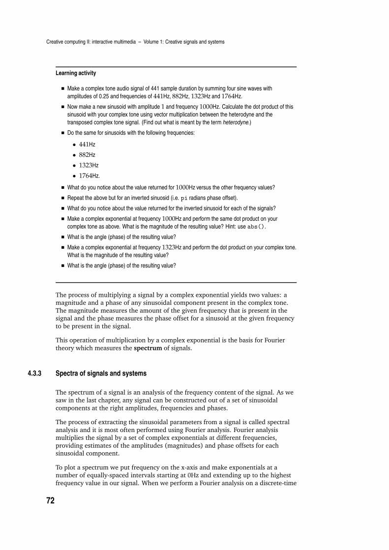
Creative computing II: interactive multimedia – Volume 1: Creative signals and systems
Learning activity
Make a complex tone audio signal of 441 sample duration by summing four sine waves with
amplitudes of 0.25 and frequencies of 441Hz, 882Hz, 1323Hz and 1764Hz.
Now make a new sinusoid with amplitude 1 and frequency 1000Hz. Calculate the dot product of this
sinusoid with your complex tone using vector multiplication between the heterodyne and the
transposed complex tone signal. (Find out what is meant by the term heterodyne.)
Do the same for sinusoids with the following frequencies:
• 441Hz• 882Hz• 1323Hz• 1764Hz.What do you notice about the value returned for 1000Hz versus the other frequency values?
Repeat the above but for an inverted sinuosid (i.e. pi radians phase offset).
What do you notice about the value returned for the inverted sinusoid for each of the signals?
Make a complex exponential at frequency 1000Hz and perform the same dot product on your
complex tone as above. What is the magnitude of the resulting value? Hint: use abs().
What is the angle (phase) of the resulting value?
Make a complex exponential at frequency 1323Hz and perform the dot product on your complex tone.
What is the magnitude of the resulting value?
What is the angle (phase) of the resulting value?
The process of multiplying a signal by a complex exponential yields two values: amagnitude and a phase of any sinusoidal component present in the complex tone.
The magnitude measures the amount of the given frequency that is present in thesignal and the phase measures the phase offset for a sinusoid at the given frequency
to be present in the signal.
This operation of multiplication by a complex exponential is the basis for Fourier
theory which measures the spectrum of signals.
4.3.3 Spectra of signals and systems
The spectrum of a signal is an analysis of the frequency content of the signal. As we
saw in the last chapter, any signal can be constructed out of a set of sinusoidal
components at the right amplitudes, frequencies and phases.
The process of extracting the sinusoidal parameters from a signal is called spectral
analysis and it is most often performed using Fourier analysis. Fourier analysismultiplies the signal by a set of complex exponentials at different frequencies,
providing estimates of the amplitudes (magnitudes) and phase offsets for eachsinusoidal component.
To plot a spectrum we put frequency on the x-axis and make exponentials at anumber of equally-spaced intervals starting at 0Hz and extending up to the highest
frequency value in our signal. When we perform a Fourier analysis on a discrete-time
72

Spectral analysis
signal it is called a discrete Fourier transform (DFT). A magnitude spectrumrepresents the relative strengths of the sinusoidal components in our signal.
We can re-construct a signal by summing together sinusoids containing the relativestrengths provided by the Fourier analysis. This reverse process is known as Fourier
synthesis.
4.3.4 Fast Fourier Transform (FFT)
The more densely we sample the frequency axis, the more time it takes to perform
the Fourier analysis. For long signals a Fourier analysis can take more time than wehave available. Fortunately, a clever algorithm was invented by Cooley and Tukey in
the 1960s that performs a discrete Fourier transform much faster than the for-loop
above.
Octave provides a function to compute the fast Fourier transform of a signal called
fft(). This function takes a signal as an argument and performs the multiplicationby a series of complex exponentials yielding a complex valued spectrum. We take the
magnitude of the resulting spectrum to find the amplitudes of the sinusoidalcomponents and we take the angle of the resulting spectrum to find the relative
phase offsets.
Spectrum of a sine wave
Figure 4.8 shows the spectrum of a sine wave. The Octave code that generated thefigure is:
t = [0:1/1000:1]; % 1s at 1000Hz sample rate
x = sin(2*pi*100*t); % 100Hz sine wave
n = 10; % how many frequency samples to take
stem([0:2/n:2-2/n],abs(fft(x(1:n))),’*’)
axis([0 2 0 6])
This example first constructs a vector of time-points at which to sample a sine wave.The sampling rate is 1000Hz. Then a signal, x, is constructed by sampling a sine
wave with frequency 100Hz which is angular frequency 2*pi*100Hz. We define nthe number of samples of the waveform to use to compute frequency estimates; thiswill be the number of frequency samples that are calculated by the FFT. The fourth
line makes a stem plot of the magnitude (abs()) FFT of one cycle of the sine wave,
i.e. 10 samples.
The number of samples in one cycle of a repeating waveform, such as a sine wave, is
called the period:
p = sr/f
Notice that in our examples the period consists of a whole number of samples.
For a sample rate sr and signal of length n, the FFT takes frequency samples of the
signal at angular frequency intervals sr/n; in this case the frequency samples arespaced by 1000/10 = 100Hz. The x-axis for the stem plot is determined by sampling
73

Creative computing II: interactive multimedia – Volume 1: Creative signals and systems
the angular frequencies 0*2*pi/(1000/10) to 10 ∗ 2 ∗ pi/(1000/10)which simplifiesto 0 to 2 ∗ pi. This way of labelling the frequency axis is called normalisedfrequency.
In normalised frequency the value 2 ∗ pi is the sample rate, the value pi is the
Nyquist frequency and all the frequency samples are spaced at angular frequencyintervals of 2 ∗ pi/n for a signal of length n.
The spectrum for frequencies greater than the Nyquist frequency is the mirror image,about pi, of the spectrum for frequencies less than the Nyquist frequency. This
symmetry in the Fourier transform is present for all real-valued signals. It is usual to
ignore the values greater than the Nyquist when interpreting a spectrum.
The most important feature of the spectrum of a sine wave is to recognise that there
is only one frequency, below the Nyquist, that has non-zero magnitude. This meansthat a sine wave has exactly one frequency component. The sine wave is the basis
for the spectrum; the spectrum tells us the amplitudes of the sine waves that wesample, at 2 ∗ pi/n intervals. All length-n signals can be constructed by summing nsine waves with amplitudes corresponding to the magnitudes of the spectrum. This
is the most remarkable fact of Fourier analysis: (almost) all signals can berepresented and reconstructed as sums of sinusoids; this was discovered by the
French mathematician Jean Baptiste Joseph Fourier in the late 1700s.
0
1
2
3
4
5
6
0 0.5 1 1.5 2
Mag
nitu
de
Frequency (multiples of pi)
Magnitude FFT of 1 cycle of 100Hz sine wav at 1000Hz sample rate
Figure 4.8: The magnitude spectrum of one cycle of a 100Hz sine with sample rate 1000Hz.
The x-axis consists of 10 frequency components spanning angular frequencies 0 to 2π. The
spectrum is symmetric around its mid-point; only frequencies from 0 to the Nyquist
frequency π are informative, the rest are due to mathematical symmetry in the Fourier
transform of real signals.
To completely represent a signal in frequency each sinusoidal frequency component
also needs a phase offset.
74

Spectral analysis
Figure 4.9 shows the phase spectrum of the same sine wave. The phase spectrum iscomputed by taking the angle() of the FFT of a signal. The phase values represent
the phase offset of each frequency component and these values are in the range −pito pi, spanning a 2 ∗ pi range. In the figure the phase angle is shown in normalized
units of pi; the y-axis is in the range −1 to 1 which means −1 ∗ pi to 1 ∗ pi.
-1
-0.5
0
0.5
1
0 0.5 1 1.5 2
Pha
se (
mul
tiple
s of
pi)
Frequency (multiples of pi)
Phase of 1 cycle of 100Hz sine wav at 1000Hz sample rate
Figure 4.9: The phase spectrum of the sine wave corresponding to Figure 4.8. The phase
spectrum is anti-symmetric about its mid-point. The phases of frequencies π to 2π are
inverted values of the phases 0 to π.
From the phase spectrum we can see that the phase of the only non-zero magnitudesinusoidal component is −π/2. This is the Fourier phase of a sine wave with −π/2phase; it corresponds to a cosine wave.
Spectrum of a cosine wave
Figure 4.10 shows the magnitude FFT of a cosine wave consisting of 10 samplescorresponding to one full cycle of the cosine wave with frequency 100Hz at a sample
rate of 1000Hz. Can you see a difference between Figure 4.10 and Figure 4.8?
Spectrum of 10 cycles of a sine wave
We already know that a sine wave, or cosine wave, is periodic which means that itrepeats and that the period of the repetition in samples is the sample rate divided by
the frequency: sr/n. How does including more samples of the signal affect the
Fourier analysis of the signal?
By setting n = 10 ∗ sr/f = 100 we can compute the Fourier transform of 10 cycles of
the sine wave. Figure 4.12 shows the Fourier transform. How is the Fouriertransform for 10 cycles different from the Fourier transform for one cycle?
75
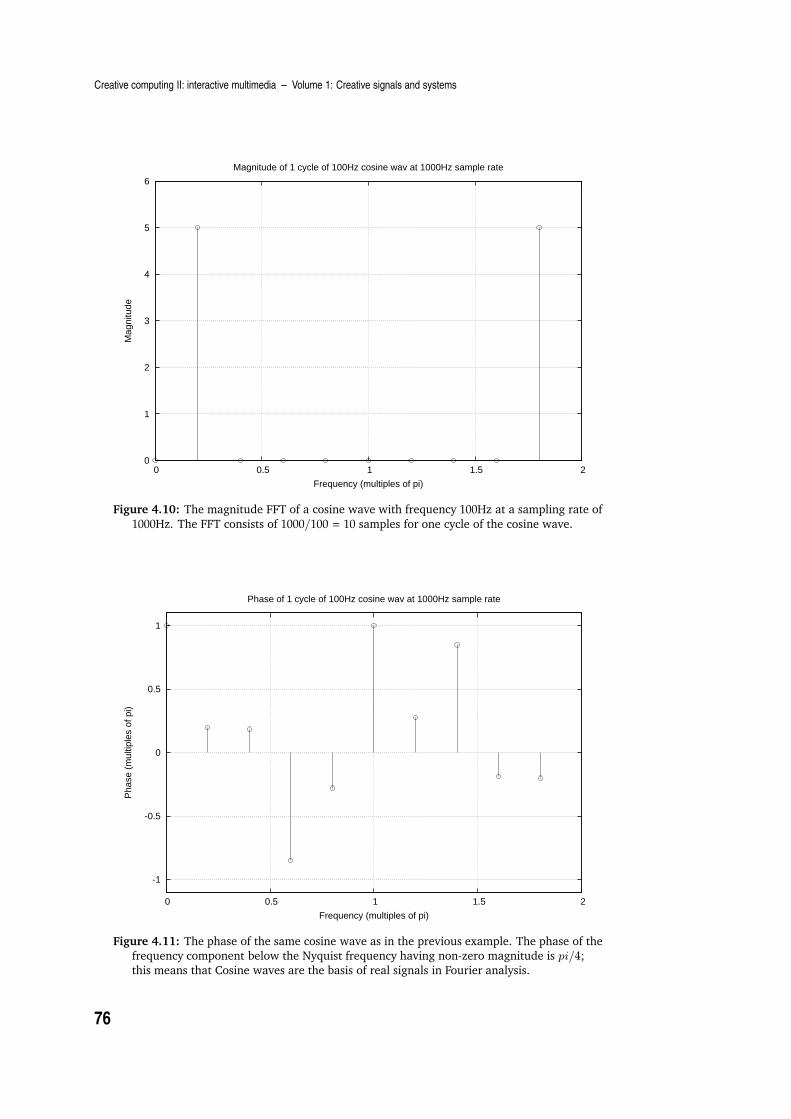
Creative computing II: interactive multimedia – Volume 1: Creative signals and systems
0
1
2
3
4
5
6
0 0.5 1 1.5 2
Mag
nitu
de
Frequency (multiples of pi)
Magnitude of 1 cycle of 100Hz cosine wav at 1000Hz sample rate
Figure 4.10: The magnitude FFT of a cosine wave with frequency 100Hz at a sampling rate of
1000Hz. The FFT consists of 1000/100 = 10 samples for one cycle of the cosine wave.
-1
-0.5
0
0.5
1
0 0.5 1 1.5 2
Pha
se (
mul
tiple
s of
pi)
Frequency (multiples of pi)
Phase of 1 cycle of 100Hz cosine wav at 1000Hz sample rate
Figure 4.11: The phase of the same cosine wave as in the previous example. The phase of the
frequency component below the Nyquist frequency having non-zero magnitude is pi/4;this means that Cosine waves are the basis of real signals in Fourier analysis.
76

Spectral analysis
0
0.1
0.2
0.3
0.4
0.5
0.6
0 0.5 1 1.5 2
RM
S E
nerg
y
Frequency (multiples of pi)
RMS Energy of 100 cycles of 100Hz cosine wav at 1000Hz sample rate
Figure 4.12: Fourier transform of 10 cycles of the sine wave.
By increasing the length of the signal to 100 samples we have not altered the
frequency content of the signal but we have altered the total energy in the signal
because energy depends on the signal’s length:
Energy =
√
√
√
√
N∑
n=1
x[n]2
To eliminate the dependency on the length of the signal we often use theroot-mean-square (RMS) energy, which divides the total energy by the length of the
signal:
RMS =
√
√
√
√
1
N
N∑
n=1
x[n]2
If we do the same for the Fourier transform, then the Magnitude spectrum divided
by the signal length will yield the same values for periodic signals with a length ofany integer multiple of the period.
77

Creative computing II: interactive multimedia – Volume 1: Creative signals and systems
Learning activity
Compute the magnitude Fourier transform of three cycles of a sine wave with frequency 400Hz and
sample rate of 1000Hz. Make a stem plot of the magnitude Fourier transform.
Compute the magnitude Fourier transform of eleven cycles of a sine wave with frequency 400Hz and
sample rate of 1000Hz. Make a stem plot of the magnitude Fourier transform.
Divide the two magnitude Fourier transforms by the length of the signals (3 and 11 cycles
respectively) and make stem plots of the results. What is the difference between the two plots?
Use the Octave commands xlabel, ylabel and title to label your plots.
By increasing the length of the signal we increase the number of frequency samplesin the Fourier transform. This means that the spacing between frequency
components that we analyse gets smaller; the Fourier analysis components are closer
together in frequency.
If we choose an integer multiple of the period of the sine wave as the signal length
then the values of the magnitude components do not change. What changes is thenumber of samples of the spectrum that we compute. Hence, for a single sine wave
the same non-zero magnitude value is reported for multiple cycles (after dividing bythe signal length) as for one cycle; but the position of this non-zero value in the
sequence of frequency samples changes because the frequency samples are more
dense. What we see are an increased number of samples of the same underlyingmagnitude spectrum.
This is also true for phase. The value of the phase for the component with non-zeromagnitude remains the same but here we see many more phase values that are
non-zero, as in Figure 4.13. These phase values are for components that do not exist
in the signal so they can essentially be ignored. We are only interested in the phasesof those components with non-zero magnitude. Again, what we see is not a different
phase spectrum, but more samples of the same underlying phase spectrum.
Spectrum of an impulse
The Fourier transform of the unit impulse also shows a fundamental property of theSpectrum:
octave:>fft([1 0 0 0 0 0 0 0])
ans =
1 + 0i 1 + 0i 1 + 0i 1 + 0i 1 + 0i 1 - 0i 1 - 0i 1 - 0i
octave:>abs(ans)
ans =
1 1 1 1 1 1 1 1
Figure 4.14 shows the unit impulse signal; notice that the signal is offset in time.
Figure 4.15 shows the spectrum of the unit impulse. These examples illustrate thatthe magnitude Fourier transform of the unit impulse is a sequence of 1s. The phase
of each component in the Fourier transform is related to the time shift of the unitimpulse.
78

Spectral analysis
-1
-0.8
-0.6
-0.4
-0.2
0
0.2
0.4
0.6
0.8
1
0 0.2 0.4 0.6 0.8 1 1.2 1.4 1.6 1.8 2
Pha
se (
mul
tiple
s of
pi)
Frequency (multiples of pi)
Phase of 100 cycles of 100Hz sine wav at 1000Hz sample rate
Figure 4.13
For the impulse in Figure 4.14 the phase is:
octave:>angle(fft([0 0 0 0 0 1 0 0 0 0 0]))
ans =
Columns 1 through 8:
0.00000 -2.85599 0.57120 -2.28479 1.14240 -1.71360 1.71360 -1.14240
Columns 9 through 11:
2.28479 -0.57120 2.85599
Note that the signal is of length 11; the phase in this example can be more
conveniently represented in units of 2 ∗ pi/11:
ans/(2*pi/11)
ans =
0 -5 1 -4 2 -3 3 -2 4 -1 5
79
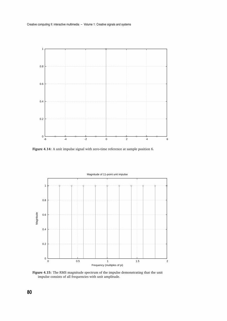
Creative computing II: interactive multimedia – Volume 1: Creative signals and systems
0
0.2
0.4
0.6
0.8
1
-6 -4 -2 0 2 4 6
Figure 4.14: A unit impulse signal with zero-time reference at sample position 6.
0
0.2
0.4
0.6
0.8
1
0 0.5 1 1.5 2
Mag
nitu
de
Frequency (multiples of pi)
Magnitude of 11-point unit impulse
Figure 4.15: The RMS magnitude spectrum of the impulse demonstrating that the unit
impulse consists of all frequencies with unit amplitude.
80

Spectral analysis
Learning activity
Make stem plots of the magnitude and phase spectra, using Fourier transforms, of one cycle of each of the
following waveforms with a sample rate of 44.1kHz and a fundamental frequency of 441Hz (Hint: one cycle
will be 44100/441 = 100 samples):
ten harmonics with amplitude (1− k/10)
ten harmonics with amplitude k/10
ten harmonics with amplitude exp(0.5 ∗ −k)
ten harmonics with amplitude exp(0.5 ∗ k)
the fundamental and even harmonics up to ten harmonics [ 1 2 4 6 8 10 ]
the fundamental and odd harmonics up to ten harmonics [ 1 3 5 7 9 ].
4.3.5 Convolution by spectrum multiplication
A further very useful property of convolution is that when we take the spectrum of
two signals, their element-wise product is the Fourier transform of their convolution.This means that taking the inverse Fourier transform, using ifft(), yields the
convolution of the two signals.
Because the FFT is an efficient way to compute the Fourier transform, the process of
computing the spectrum, performing multiplication and taking the inverse Fourier
transform is more efficient and therefore takes less time than the process ofconvolution using conv().
Here are some examples of convolution using FFTs. The first example is convolutionof a signal by the unit delay.
sig = [1 2 3 4 5 6 5 4 3 2 1];
d = [0 1]; S = fft(sig, length(sig)+length(d)-1); D = fft(d,
length(sig)+length(d)-1); X = S .* D; x = ifft(X); sig
sig =
1 2 3 4 5 6 5 4 3 2 1
fix(real(x)) ans =
0 1 2 3 4 5 6 5 4 3 2 1
The second example illustrates the use of the FFT to perform low-pass filtering of asignal using the 2-point averaging filter [0.5 0.5]:
sig = rand(1,10)*2-1;
d = [0.5 0.5]; S = fft(sig, length(sig)+length(d)-1); D = fft(d,
length(sig)+length(d)-1); X = S .* D; x = ifft(X); sig = Columns 1
through 7:
0.660514 -0.287672 0.092979 0.954095 0.137672 0.845794 -0.120167
Columns 8 through 10:
0.920592 -0.715481 -0.512909
x x =
Columns 1 through 7:
0.330257 0.186421 -0.097346 0.523537 0.545883 0.491733 0.362814
81
Creative computing II: interactive multimedia – Volume 1: Creative signals and systems
Columns 8 through 11:
0.400213 0.102555 -0.614195 -0.256454
conv(sig,d) ans =
Columns 1 through 7:
0.330257 0.186421 -0.097346 0.523537 0.545883 0.491733 0.362814
Columns 8 through 11:
0.400213 0.102555 -0.614195 -0.256454
There are many uses for Fourier transforms: in this chapter we have used them foranalysing spectra of signals to see their constituent frequency components and for an
alternative implementation of the convolution operation.
Building upon the knowledge that you have gained about systems, convolution,
Fourier representations and transformation by Fourier representations, there is afinal observation that we can make.
LTI systems have the unique property that complex exponentials presented at theinput are passed through the system and multiplied by the frequency components of
the impulse response of the system. There can be no new frequency components
added by a linear system; instead, existing frequency components can be attenuated,amplified or delayed. Therefore all discrete-time systems are combinations of the
simple operation of scaling and delaying individual sinusoidal components that are
summed together to form the system response to the input.
In other words, sinusoids presented at the input to a system are also present at the
output; but they can be scaled and/or delayed. Because all signals can berepresented as sums of sinusoids, all system responses can be decomposed into their
individual scaled and delayed sinusoids that are summed back together to form thefinal signal. For this reason it is said that Complex Exponentials are Eigenfunctions of
Linear Time Invariant Systems. An Eigenfunction is a signal, in this case a sinusoid,
that passes through a system with its basic shape unchanged; and LTI systems do notchange the shape of sinusoids, they simply scale them and shift them in time.
4.4 Summary and learning outcomes
This chapter first looked at linear time invariant (LTI) systems and their properties.
The impulse response was introduced as a complete characterisation of LTI systems
that is used to implement system transformations on signals using the convolutionoperator.
The convolution operator was shown to be a way to combine a signal with itself by
delaying and scaling. This produces a transformation of the signal that is often
called filtering. The operations of delay and low-pass filtering were introduced.
Representation of sinusoidal signals by complex exponentials was introduced
leading to the representation known as the spectrum. The Fourier transform, usingthe FFT, was then discussed as a means for computing spectra as well as its
implementation in the Octave programming language. It was then illustrated that
the Fourier transforms of a signal and a system can be multiplied to produce theFourier transform of the convolution of the two signals. By taking the inverse Fourier
transform of this product the convolved, or filtered, signal is produced.
Not only is the Fourier transform a useful analysis tool for inspecting the sinusoidal
components of signals and systems, but it can be a more efficient method for
82

Exercises
performing convolution than computation by direct means (e.g. using conv()). Forthese reasons the Fourier transform, and the complex exponential representation of
signals and systems, are very important in the study of signal processing.
With a knowledge of the contents of this chapter and its directed reading and
activities, you should be able to:
describe what an LTI system is
discuss the impulse response and its importance in signal processing
describe what convolution is and how it is used, as well as being able to perform
convolution on signals using Octave
describe the basic theory of Fourier analysis, and in particular the use of the FastFourier Transform in digital signal processing
describe spectral analysis and how signals are made up of sinusoidal waveforms.
4.5 Exercises
In addition to the exercises listed below, you should attempt all of the learningactivities throughout this chapter, to enhance your understanding of the material.
1. What is the difference between a signal and a system?
2. What is meant by the term ‘impulse response’? What is the impulse response of a
room?
3. What is Fourier analysis? Discuss the use of Fourier analysis for both analogueand digital signals. In particular, describe how the analysis might differ for these
two types of signals.
4. What is a Fourier Transform? Can a Fourier Transform be applied to bothanalogue and digital signals? What is a Fast Fourier Transform? Is this
applicable to both analogue and digital signals?
5. What is convolution? What is the relationship between convolution and the FFT?
83

Creative computing II: interactive multimedia – Volume 1: Creative signals and systems
84
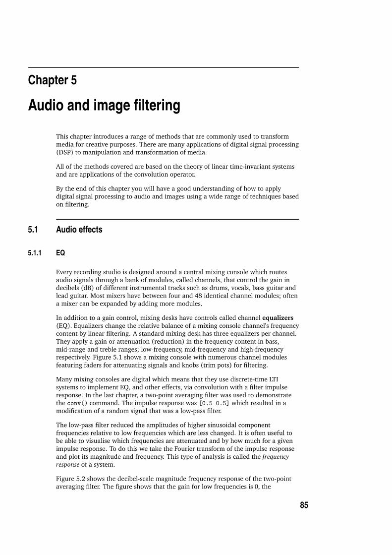
Chapter 5
Audio and image filtering
This chapter introduces a range of methods that are commonly used to transform
media for creative purposes. There are many applications of digital signal processing(DSP) to manipulation and transformation of media.
All of the methods covered are based on the theory of linear time-invariant systemsand are applications of the convolution operator.
By the end of this chapter you will have a good understanding of how to applydigital signal processing to audio and images using a wide range of techniques based
on filtering.
5.1 Audio effects
5.1.1 EQ
Every recording studio is designed around a central mixing console which routes
audio signals through a bank of modules, called channels, that control the gain in
decibels (dB) of different instrumental tracks such as drums, vocals, bass guitar andlead guitar. Most mixers have between four and 48 identical channel modules; often
a mixer can be expanded by adding more modules.
In addition to a gain control, mixing desks have controls called channel equalizers(EQ). Equalizers change the relative balance of a mixing console channel’s frequencycontent by linear filtering. A standard mixing desk has three equalizers per channel.
They apply a gain or attenuation (reduction) in the frequency content in bass,
mid-range and treble ranges; low-frequency, mid-frequency and high-frequencyrespectively. Figure 5.1 shows a mixing console with numerous channel modules
featuring faders for attenuating signals and knobs (trim pots) for filtering.
Many mixing consoles are digital which means that they use discrete-time LTI
systems to implement EQ, and other effects, via convolution with a filter impulse
response. In the last chapter, a two-point averaging filter was used to demonstratethe conv() command. The impulse response was [0.5 0.5] which resulted in a
modification of a random signal that was a low-pass filter.
The low-pass filter reduced the amplitudes of higher sinusoidal component
frequencies relative to low frequencies which are less changed. It is often useful tobe able to visualise which frequencies are attenuated and by how much for a given
impulse response. To do this we take the Fourier transform of the impulse response
and plot its magnitude and frequency. This type of analysis is called the frequencyresponse of a system.
Figure 5.2 shows the decibel-scale magnitude frequency response of the two-pointaveraging filter. The figure shows that the gain for low frequencies is 0, the
85

Creative computing II: interactive multimedia – Volume 1: Creative signals and systems
Figure 5.1: A contemporary mixing console features long-throw faders for attenuating an
input signal and a set of equalizers (EQ) for altering the relative balance of the frequency
content of each channel’s audio signal. The input channels are routed to the output,
typically stereo, via an audio buss.
pass-band, and that the gain slopes gradually to around −10dB for high frequenciesabove 0.8π angular frequency. Using the decibel equation from Chapter 3 the gain is
expressed in meaningful terms for human perception. Recall that a gain of −10dB
corresponds to about half the perceived loudness relative to zero. For an input signalwith equal strength low and high frequencies, after filtering the high frequencies
would sound less than half as loud as the low frequencies in this example. The
frequency range that remains unaltered by a filter is called the pass-band and therange that is attenuated is called the stop band.
In addition to the magnitude response, it is often important to know the phaseresponse of a filter. If the phase response is very discontinuous across the frequency
range this can lead to a phenomenon called phase distortion; which can lead tounwanted artefacts such as blurring of transients (attacks) in the audio signal. The
lower graph of Figure 5.2 shows the phase response of the two-point averaging filter
which is linear. A desirable property of digital filters used for audio filtering is thatthey are close to linear phase. Symmetric FIR filters–i.e. those with values that
mirror each other around a centre-point–have linear phase response. Linear phase
means that all frequencies are delayed by the same amount, so there is no phasedispersion.
By inspection of the diagrams of the frequency response of the two-point averaging
filter we can see that the effect on frequencies is limited until the very highest
frequencies. To create a filter with greater attenuation for mid-range frequencies afilter with a longer impulse response must be created. The following section
describes how to design such filters in Octave.
86
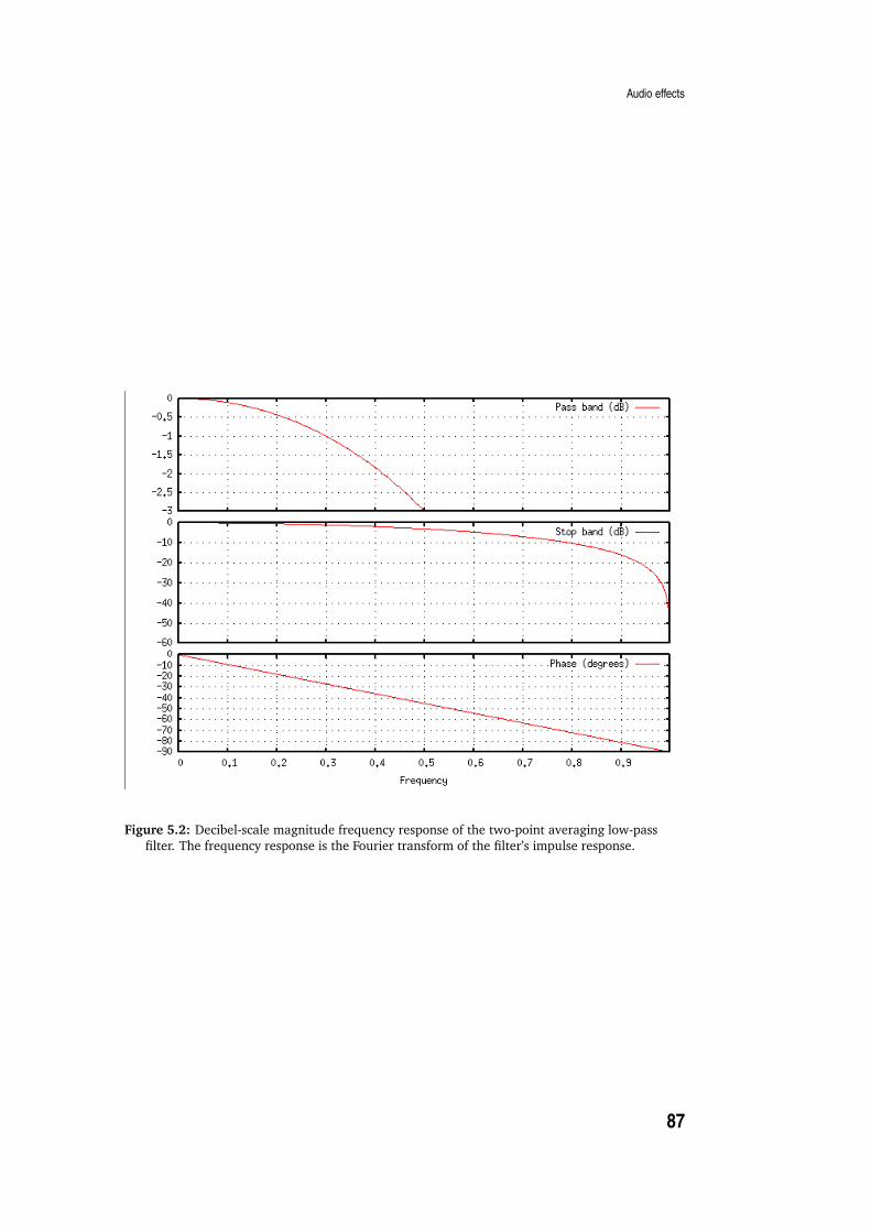
Audio effects
Figure 5.2: Decibel-scale magnitude frequency response of the two-point averaging low-pass
filter. The frequency response is the Fourier transform of the filter’s impulse response.
87
Creative computing II: interactive multimedia – Volume 1: Creative signals and systems
5.1.2 FIR filter design
The filters encountered so far have impulse responses with a finite number of
non-zero samples; the two-point averaging filter had an impulse response of lengthtwo. Filters that have a determinate length are called finite impulse response filters
(FIR); in this chapter we will focus exclusively on these. A different class of filtershave an infinite impulse response (IIR). IIR filters have exactly the same properties
as all LTI systems, except their impulse response is more complicated to describe
than those of FIR filters.
Design of an FIR filter requires a cutoff frequency and a filter order. For an ideal
low-pass filter, the cutoff is the frequency above which sinusoidal components arerejected; that is, they have a gain of 0. Conversely, for an ideal high-pass filter the
cutoff is that frequency where sinusoidal components of the signal are admitted witha gain of 1; below the cutoff the gain is 0.
Due to mathematical properties of the frequency domain, the ideal low-pass andhi-pass filters are not achievable. There is always a region of the frequency space
that is a transition between the pass-band and the stop band; this region is called the
transition band.
Figure 5.3: Decibel-scale frequency response of a 100-point FIR filter designed using fir1()
High-pass filter
A high-pass filter is one for which the stop-band is the low frequencies and thepass-band is the high frequencies. An example of a high-pass filter is the two-point
differentiating filter [-1 1] or [1 -1]. The frequency response of the two-point
88

Audio effects
differentiating filter is shown in Figure 5.4.
Figure 5.4: The decibel-scale frequency response of the two-point high-pass filter [1 -1]
plotted using an absolute frequency axis.
Just as with the low-pass FIR filter examples above we construct high-pass filters byspecifying a cutoff frequency. The meaning of the cutoff frequency is reversed
relative to low-pass filters; it is the frequency at which the stop band ends and thepass-band starts.
Band-pass filter
One of the properties of LTI systems is that they can be composed to form an
aggregate filter. The aggregate filter has an impulse response that is the convolutionof the impulse responses of the individual filters. The convolution of two signals or,
equivalently, impulse responses, is the element-wise product of their frequency
responses (i.e. their complex multiplication in the frequency domain).
Hence, we can combine filters by multiplying their complex-valued frequency
responses. Figure 5.6 shows a band-pass filter that rejects both low frequencies andhigh frequencies but admits frequency components that are in a centre pass-band.
Band-pass filters are constructed out of the composition of a low-pass and ahigh-pass filter. The low-frequency stop-band is determined by the cutoff frequency
of a high-pass filter, and the high-frequency stop-band is determined by the low-pass
filter cutoff. The convolution of the two impulse responses produces the band-passfilter.
89
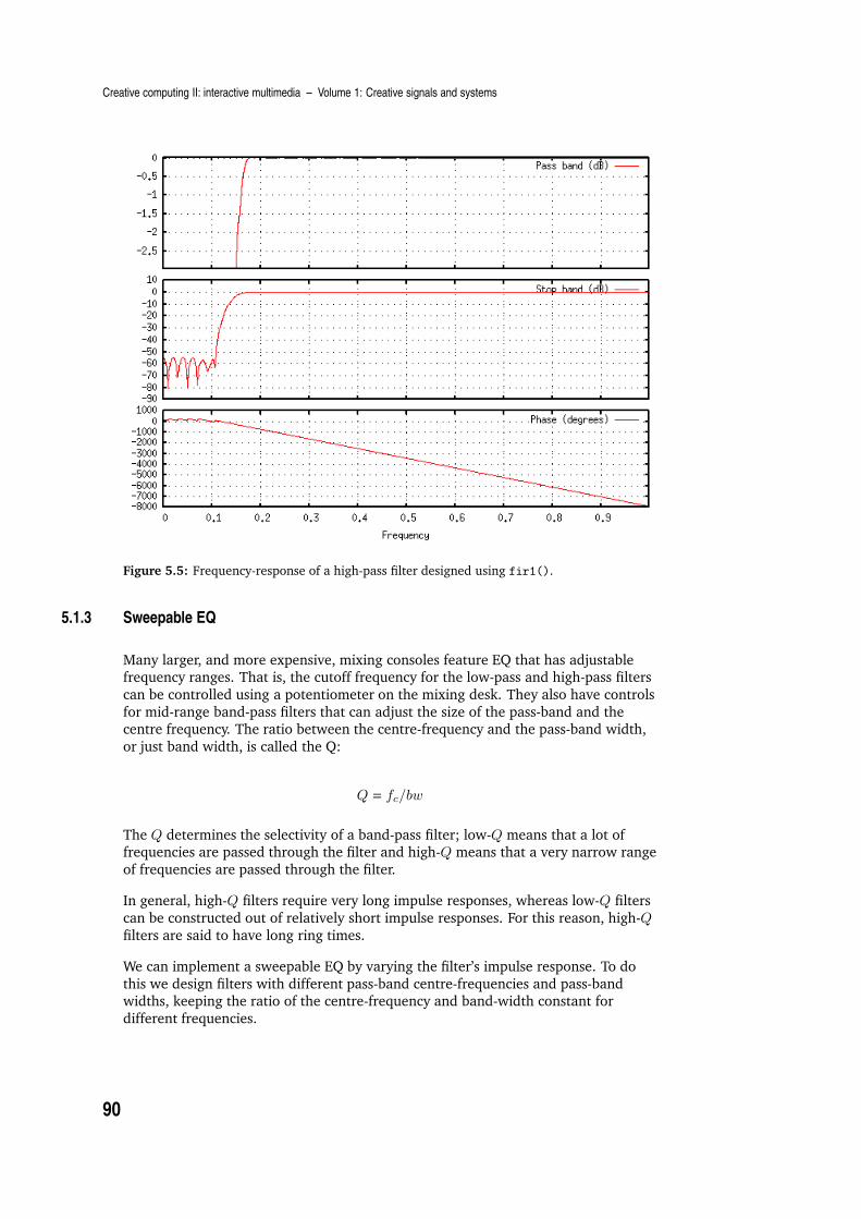
Creative computing II: interactive multimedia – Volume 1: Creative signals and systems
Figure 5.5: Frequency-response of a high-pass filter designed using fir1().
5.1.3 Sweepable EQ
Many larger, and more expensive, mixing consoles feature EQ that has adjustablefrequency ranges. That is, the cutoff frequency for the low-pass and high-pass filters
can be controlled using a potentiometer on the mixing desk. They also have controls
for mid-range band-pass filters that can adjust the size of the pass-band and thecentre frequency. The ratio between the centre-frequency and the pass-band width,
or just band width, is called the Q:
Q = fc/bw
The Q determines the selectivity of a band-pass filter; low-Q means that a lot offrequencies are passed through the filter and high-Q means that a very narrow range
of frequencies are passed through the filter.
In general, high-Q filters require very long impulse responses, whereas low-Q filters
can be constructed out of relatively short impulse responses. For this reason, high-Qfilters are said to have long ring times.
We can implement a sweepable EQ by varying the filter’s impulse response. To do
this we design filters with different pass-band centre-frequencies and pass-bandwidths, keeping the ratio of the centre-frequency and band-width constant for
different frequencies.
90

Audio effects
Figure 5.6: Frequency-response of a band-pass filter designed by convolving the impulse
responses of a low-pass filter and a high-pass filter designed using fir1(). The pass-band
is from 900Hz to 1100Hz normalised to angular-frequency (2 ∗ pi ∗ 900/44100 and
2 ∗ pi ∗ 1100/44100).
91

Creative computing II: interactive multimedia – Volume 1: Creative signals and systems
Learning activity
Construct the following band-pass filters for a sample rate of 44100Hz with a Q of 10 by convolving a
low-pass and high-pass 100th-order FIR filter in each case:
centre-frequency 1000Hz band-width 100Hz
centre-frequency 2000Hz band-width 200Hz
centre-frequency 100Hz band-width 10Hz.
Plot the impulse responses of your filters, i.e. the vector returned by fir1(), using Octave’s freqz()
function. Save your plots using the print() function.
5.1.4 Subtractive synthesis
Among the first creative uses of digital filtering was music synthesis. Early music
synthesizers, such as those invented by Bob Moog in the 1960s, used a techniquecalled subtractive synthesis to create different musical timbres, meaning tone
colours or sound qualities.
A rich source waveform is generated at a given musical pitch, which has a
fundamental frequency corresponding to the key pressed on a piano-like keyboard,and this waveform is filtered to create the different timbres. Musical pitch is relative
to a reference frequency which is usually chosen to be Concert Pitch (A 440Hz). We
use the lowest instance of this pitch (A 55Hz) as the base frequency from which wegenerate the frequencies of all other musical pitches. Given a reference frequency,
the frequencies of the semitones of Western music scales are given by the relation:
fk = 55 ∗ 2k/12
where k is the note number, or number of semitones, along a standard music
keyboard. We can hear the basic principles of subtractive synthesis by low-pass or
band-pass filtering a Helmholtz waveform, consisting of many partials.
For musical sounds, the waveform is periodic, meaning that the same wave repeats
every frequency cycle at the given pitch; this means that the spectrum is alsoperiodic with partials spaced from 0Hz every fk Hz.
To create a frequency-rich waveform, we assume a sample rate of 44.1kHz and a
relatively low fundamental frequency of 100Hz. We can construct a Helmholtz
waveform using the spectrum and inverse FFT:
sr=44100;
X = zeros(1,44100); % make Spectrum vector X(101:100:22050)=1; %
Impulse train in spectrum spaced every 100Hz
X(44100:-1:22051)=X(1:22050); % Symmetric spectrum x=real(ifft(X)); %
Construct waveform by inverse Fourier transform plot(x(1:4410)) % Plot
10 cycles of the waveform
92
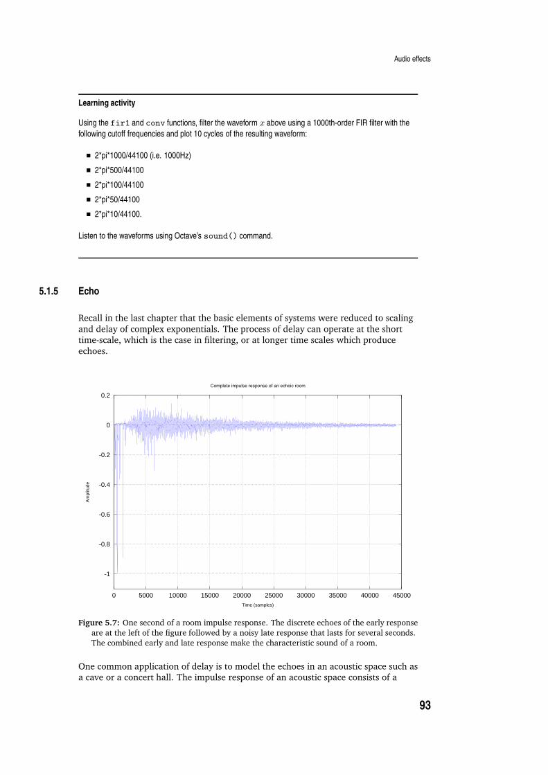
Audio effects
Learning activity
Using the fir1 and conv functions, filter the waveform x above using a 1000th-order FIR filter with thefollowing cutoff frequencies and plot 10 cycles of the resulting waveform:
2*pi*1000/44100 (i.e. 1000Hz)
2*pi*500/44100
2*pi*100/44100
2*pi*50/44100
2*pi*10/44100.
Listen to the waveforms using Octave’s sound() command.
5.1.5 Echo
Recall in the last chapter that the basic elements of systems were reduced to scaling
and delay of complex exponentials. The process of delay can operate at the shorttime-scale, which is the case in filtering, or at longer time scales which produce
echoes.
-1
-0.8
-0.6
-0.4
-0.2
0
0.2
0 5000 10000 15000 20000 25000 30000 35000 40000 45000
Am
plitu
de
Time (samples)
Complete impulse response of an echoic room
Figure 5.7: One second of a room impulse response. The discrete echoes of the early response
are at the left of the figure followed by a noisy late response that lasts for several seconds.
The combined early and late response make the characteristic sound of a room.
One common application of delay is to model the echoes in an acoustic space such asa cave or a concert hall. The impulse response of an acoustic space consists of a
93

Creative computing II: interactive multimedia – Volume 1: Creative signals and systems
decaying set of impulses spaced at relatively long intervals, when compared withfilter impulse responses. Figure 5.7 shows the impulse response of a concert hall
(the impulse is usually a large high-pressure balloon burst and the response isrecorded by a microphone in the room).
-1
-0.8
-0.6
-0.4
-0.2
0
0 500 1000 1500 2000
Am
plitu
de
Time (samples)
Early response of an echoic room
Figure 5.8: Early response of a room measured at a sample rate of 44100Hz. The figure
shows about 120
th of a second of the room’s impulse response. Five distinct groups of
echoes can be seen in the figure; the timings of these echoes provide a strong acoustic cue
for the size of the room.
Figure 5.8 shows the first part of the room response. This is called the early responseand it is due to the echoes caused by the walls, floor and ceiling. Impulses at the
same position in the room cause the same set of echoes to occur. However, when the
impulse is produced at a different location the echo response changes. This is due tothe physical action of the impulse wave travelling in the room; the reflections of the
wave to the microphone are determined by the room’s geometry. Hence an echoic
impulse response is determined by the spatial geometry of the architecture. For thisreason, modelling echoes in room responses is part of the field called acoustics.
Echoes feature prominently in many kinds of music and special effects. In the 1960sthe Dub music of Kingston, Jamaica, featured prominent echoes on the vocal track of
dance hall music records. In the 1970s echoes were prominent in progressive rockmusic and they feature heavily on many dance music and electronic music tracks of
the 1980s and 1990s.
Echoes can be used to construct rhythms; a regular beat can be made by creating an
echo at equally spaced intervals. This is an effect that is used on many dance music
tracks.
94

Audio effects
Learning activity
The sound files required in this activity will be available for download from the student website
http://www.londonexternal.ac.uk/current students/programme resources
/cis/index.shtml.
Load the echo1.wav soundfile example into Octave.
Load the piano1.wav soundfile example into Octave and convolve the two signals using Octave’s
conv function.
Listen to the original piano1 sound, and then listen to the resulting audio using Octave’s playaudio
function.
What do you hear if you listen to the echo1 sound on its own?
5.1.6 Reverberation
Figure 5.7 shows one second of the room response corresponding to the earlyresponse above. Here we see that after the initial echoes there is a noisy decaying
signal present in the impulse response. This is the part of the room’s response known
as reverberation and it is caused by the rapid build-up of many echoes as the initialechoes get reflected around the room multiple times each. The noisy late response is
a characteristic of large spaces and it is a very important perceptual cue for the spacethat sounds occupy.
The late response of a room can also be modelled using FIR filters; but typically verylong FIR filters are needed. For example, in a large space, the impulse response can
be as long as 20 seconds before the impulse decays below the threshold of hearing,
typically set to −60dB from the initial impulse. At a sample rate of 44.1kHz that is882,000 samples for the impulse response.
It is especially important when using long impulse responses to perform theconvolution using an efficient method such as spectral multiplication via the FFT.
In the following learning activity you will use the full impulse response of a realroom to change the acoustic image of a sound so that it is perceived as localized in a
concert hall instead of as a dry source.
Learning activity
The sound files required in this activity will be available for download from the student website
http://www.londonexternal.ac.uk/current students/programme resources/
cis/index.shtml.
Load the reverb1.wav soundfile example into Octave. This signal is the room impulse response
shown in Figure 5.7.
Load the piano1.wav soundfile example into Octave and convolve the two signals using Octave’s
conv function.
Listen to the original piano1 sound then listen to the resulting audio using Octave’s playaudio function.
What do you hear if you just listen to the reverb1 sound?
95
Creative computing II: interactive multimedia – Volume 1: Creative signals and systems
About how long does the convolution computation take?
Now try using the FFT method of convolution instead of using conv.
How much faster is the FFT-based method?
5.1.7 Resampling
Sometimes it is useful to alter the sample rate of a signal relative to the original rate.
This process is called resampling. For audio synthesis this has the effect of changing
both the perceived musical pitch and the duration of the signal. As such, the processof resampling is a very important one in music synthesis.
The Fairlight sampling synthesizer was the first commercial digital musicalinstrument to employ sampling to emulate real musical instruments. Other
instruments followed including the Synclavier and the Emulator. The idea of
sampling became prominent in the 1980s and was widely used in pop music, musicfor film and television and in experimental electronic and computer music.
One of the design constraints in building a sampling synthesizer is the amount ofcomputer memory needed to store the samples. The access to the sample had to be
rapid, whenever a key was pressed, so they had to be stored in random accessmemory rather than on disk during a performance.
At the time these instruments were designed, random access memory was veryexpensive; and sampling rates had to be at least 32kHz for the sounds to have high
enough frequencies (16kHz) to be of a high fidelity for musicians to use.
Take, for example, a piano sound produced by a sampling synthesizer. There are 88
keys on a standard piano. The idea behind sampling is to record each note on the
piano separately and to play back these recordings when triggered from a keyboardadjusting the loudness relative to the velocity of the key stroke. A piano sound is
very long; if we hold the note it can easily last 30 seconds. One trick was to loop thesample after the initial attack portion of the sound until the key was released.
Another trick was to only sample every few notes (say every four) and to use pitch
shifting of the samples to generate the notes in-between.
The resample function takes three arguments: the signal to be resampled, the
interpolation factor p and the decimation factor q. The last two arguments arepositive integers. The ratio between p and q, i.e. p
q , is the resampling factor. For
example, resampling with p=1 and q=2 gives a factor of 12; the resampling will be to
half the sample rate of the original.
The change in sample rate alters the frequency content and duration of the signal
when it is played back at the original sampling rate. For example, a sine wave withfrequency 440Hz at a sample rate of 44.1kHz that is resampled to 22.05kHz and
played back at 44.1kHz will sound at 880Hz, or double the original frequency. This
is called down-sampling or decimation. The converse is also true; if the original440Hz sine wave is resampled to 88.2kHz and played back at 44.1kHz then it will
sound at 220Hz. This is called up-sampling, or interpolation.
The following example illustrates the use of Octave’s resample function to alter the
pitch of a sound to play a chromatic musical scale:
96
Audio effects
octave>[x,sr] = wavread(’sounds/pianoC5.wav’);
octave>sr
ans = 44100
octave>playaudio(x); % listen to the original
octave>y = resample(x, 1, 2); % resample to 1/2 the frequency
octave>playaudio(y); % listen to the resampled
octave>for k = 0:11 % make a musical scale
octave>y = resample(x, 2(̂k/12), 1);
octave>playaudio(y)
octave>endfor
Learning activity
What is the length, in samples, of the original piano sound above?
Make a table of the lengths of the resampled versions of the piano sound.
What is the mathematical relationship between the length of the resampled signal and the resampling factorpq ?
Band-limited resampling
Up-sampling and down-sampling processes are built upon filtering. These processes
are called band-limited resampling because they use low-pass filtering
(band-limiting) to ensure that no new frequency components are added to the signalwhen applying the interpolation and decimation steps.
For band-limited interpolation, the signal is first extended by inserting p-1 zerosbetween the original samples. Low-pass filtering must be used to avoid aliasing at
the new sample rate; the cut-off frequency is equal to the Nyquist of the originalsample rate. Figure 5.9 illustrates the steps that make up band-limited interpolation.
For down-sampling, a low-pass filter is applied first with cut-off frequency equal tothe Nyquist of the new sample rate then q-1 samples are removed after every qth
sample.
For resampling a ratio pq , both of the above operations are applied in the order of
interpolation followed by decimation. In practice, only one low-pass filter is required
when performing both steps together: that is the convolution of the two filters usedin the separate interpolation and decimation steps.
97

Creative computing II: interactive multimedia – Volume 1: Creative signals and systems
-1
-0.5
0
0.5
1
2 4 6 8 10 12 14 16 18 20
Am
plitu
de
20 samples of a signal with sample rate SR
-1-0.8-0.6-0.4-0.2
00.20.40.60.8
5 10 15 20 25 30 35 40
Am
plitu
de
Zeros inserted between original samples
-0.5-0.4-0.3-0.2-0.1
00.10.20.30.4
5 10 15 20 25 30 35 40
Am
plitu
de
Time (samples)
Low-pass filtered with original Nyquist frequency as cutoff. New sample rate is 2*SR
Figure 5.9: Example of band-limited interpolation (up-sampling). An original signal with
sample rate SR is interpolated by a factor of 2 by inserting one zero between each original
sample and low-pass filtering the new signal with cutoff frequency π
2, the original signal’s
Nyquist frequency. The new signal is twice the length of the original signal and would
need to be played back at twice the sample rate of the original to sound the same.
98

Image filtering
Learning activity
Without using Octave’s resample function, resample the piano signal above by each of the following
interpolation/decimation ratios:
p=3, q=1
p=1, q=2
p=4, q=3
p=1, q=8
p=1, q=16.
Listen to the resulting signals at the original sample rate (44.1kHz). Compare your sounds with Octave’s
resample function. If they don’t sound almost identical there may be a problem with your
interpolation/decimation and filtering method.
5.2 Image filtering
Digital images can be created and transformed using the same signal processing
tools as audio signals. The major difference is that an image has two independent
variables instead of one. These are spatial dimensions, an x-axis and a y-axis. Eachpixel in an image is labelled with an (x,y) index in a similar way to audio signals
which are labelled with only a single time axis.
To represent images a two-dimensional data structure is needed. The
two-dimensional generalisation of vectors are matrices. The following sectiondescribes the basic operations in Octave on matrices.
5.2.1 Matrices
Two or more vectors of the same size can be combined to make a matrix. A matrix issimply a collection of vectors, with some specific operations that are allowed upon
them as you will learn below.
There are several ways to construct a matrix in octave:
Matrix creation
A matrix can be created by combining vectors of the same length into a single
structure. This is achieved in Octave using the bracket [] and semicolon ; operators:
The bracket notation indicates that the enclosed values form a matrix. The
semicolon notation separates the rows of the matrix. The following are examples ofmatrix construction in Octave:
octave:>[1 2 3;4 5 6]
ans =
99

Creative computing II: interactive multimedia – Volume 1: Creative signals and systems
1 2 3
4 5 6
Here, a matrix is formed out of two rows consisting of three columns. Thus thematrix dimensions are 2× 3; two rows and three columns. The rows and columns
can each be any length as long as every contained vector is the same length. Thefollowing example is a matrix with three rows and two columns:
octave:>mymatrix = [1 2; 3 4; 5 6]
mymatrix =
1 2
3 4
5 6
Notice that the semicolon “;” operator separates the rows. This example showsassignment of the resulting matrix to a variable, mymatrix.
Learning activity
Construct the following matrices:
4 x 3 matrix consisting of integer multiples of the vector [1 2 3].
5 x 5 matrix consisting of the numbers 1 . . . 25
A matrix with rows of different lengths (unequal column counts).
What happens when you try to construct the third matrix above? Why?
Some useful matrix initialisation methods are provided in Octave for convenience.The two that are possibly the most useful for image processing are the functions
zeros() and ones(). These both take two arguments, the number of rows and
columns to make respectively, and they fill the resulting matrix with the value zeroor one:
octave:>zeros(2,3)
ans =
0 0 0
0 0 0
octave:> ones(7,2)
ans =
1 1
1 1
1 1
1 1
1 1
1 1
1 1
One interesting matrix-generating function in Octave is the magic square constructor
magic(). The function takes one argument, the row and column dimension, and
returns a matrix such that every row, column and main diagonal adds up to the samevalue:
octave:20> M5 = magic(5)
100
Image filtering
M5 =
17 24 1 8 15
23 5 7 14 16
4 6 13 20 22
10 12 19 21 3
11 18 25 2 9 octave:>sum(M5) % sum down the columns
ans =
65 65 65 65 65
octave:>sum(M5,2) % sum along the rows
ans =
65 65 65 65 65
octave:>sum(M5)́ % also sums along the rows
ans =
65 65 65 65 65
octave:> diag(M5) % extract the main diagonal
ans =
17
5
13
21
9
octave:> sum(diag(M5))
ans = 65
To get the backwards diagonal, from the top right to lower left of the matrix, we takethe diag() of the matrix flipped left-to-right using the fliplr() function: octave:>
fliplr(M5)
ans =
15 8 1 24 17
16 14 7 5 23
22 20 13 6 4
3 21 19 12 10
9 2 25 18 11
octave:31> diag(fliplr(M))
ans =
15
14
13
12
11
octave:32> sum(diag(fliplr(M)))
ans = 65
We have now verified that every row, column and diagonal adds up to the samevalue: 65.
101

Creative computing II: interactive multimedia – Volume 1: Creative signals and systems
Learning activity
Calculate the sums of the rows, columns and two main diagonals of the following matrices:
magic(3)
magic(11)
rand(10).
Matrix operations
Matrix operations are similar to vector operations in Octave.
Adding a scalar to a matrix adds the scalar value to all the individual values of the
matrix:
octave:4> ones(3,2) + 2
ans =
3 3
3 3
3 3
The same is true of subtraction:octave:49> magic(3) - 1.5 ans =
6.50000 -0.50000 4.50000
1.50000 3.50000 5.50000
2.50000 7.50000 0.50000
Here the resulting matrix contains floating point and negative values. We can alsomake a complex-valued matrix by adding a complex number to a real-valued matrix:
octave:>magic(3) + i*pi
ans =
8.0000 + 3.1416i 1.0000 + 3.1416i 6.0000 + 3.1416i
3.0000 + 3.1416i 5.0000 + 3.1416i 7.0000 + 3.1416i
4.0000 + 3.1416i 9.0000 + 3.1416i 2.0000 + 3.1416i
Matrix-scalar multiplication similarly yields the product of the individual matrixelements and the scalar value:
octave:>mymatrix = ones(4,3) * 1.61-3.14i
mymatrix =
1.6100 - 3.1400i 1.6100 - 3.1400i 1.6100 - 3.1400i
1.6100 - 3.1400i 1.6100 - 3.1400i 1.6100 - 3.1400i
1.6100 - 3.1400i 1.6100 - 3.1400i 1.6100 - 3.1400i
1.6100 - 3.1400i 1.6100 - 3.1400i 1.6100 - 3.1400i
Here, the resulting matrix consists of all complex-valued elements. We can pass a
matrix as an argument to any of Octave’s functions and the results will also be a
matrix:
octave:>abs(mymatrix)
ans =
3.5287 3.5287 3.5287
102

Image filtering
3.5287 3.5287 3.5287
3.5287 3.5287 3.5287
3.5287 3.5287 3.5287
octave:>angle(mymatrix)
ans =
-1.0970 -1.0970 -1.0970
-1.0970 -1.0970 -1.0970
-1.0970 -1.0970 -1.0970
-1.0970 -1.0970 -1.0970
Addition of two matrices is possible only if they have the same number of rows and
columns:
octave:>R = rand(2,3) % A 2× 3 matrix of random values
R =
0.967629 0.254644 0.565806
0.656365 0.876986 0.053914
octave:>a = [1 2 3]
a =
1 2 3
octave:> R + a % Attempt to add a matrix and a vector with different
dimensions
error: operator +: nonconformant arguments (op1 is 2x3, op2 is 1x3)
error: evaluating binary operator ‘+’ near line 4, column 3
The problem here is that we cannot add a vector to a matrix because they have
different dimensions. But we can form a matrix out of the vector so that it has the
same dimensions as the matrix and then perform the addition:
octave:>a = [1 2 3;4 5 6]
a =
1 2 3
4 5 6
octave:>R + a
ans =
1.9676 2.2546 3.5658
4.6564 5.8770 6.0539
Multiplication between matrices has two forms: element-wise multiplication andmatrix multiplication. The rules for element-wise multiplication, or division, are the
same as for addition and subtraction. Two matrices can be multiplied element-wise
if they both have the same row and column dimensions:
R .* a % element-wise multiplication
ans =
0.96763 0.50929 1.69742
2.62546 4.38493 0.32348
octave:67> R ./ a
ans =
0.9676290 0.1273218 0.1886019
0.1640912 0.1753972 0.0089856
The addition operations above are associative and commutative:
associative:A + (B + C) = (A +B) + C,
103
Creative computing II: interactive multimedia – Volume 1: Creative signals and systems
commutative:A +B = B +A
The element-wise multiplication operation is associative, distributive and
commutative:
associative:A. ∗ (B. ∗ C) = (A. ∗ B). ∗ C
distributive:A. ∗ (B + C) = A. ∗ B +A. ∗ C
commutative:A. ∗ B = B. ∗ A
However, matrix multiplication is not associative or commutative. The rules for
matrix multiplication are similar to the rules for vector multiplication. Recall that
the inner dimensions of two vectors A,B had to match for multiplication: i.e.columns(A) == rows(B) must be true for A*B to be possible. The same rule applies
to matrix multiplication:
octave:> R = rand(4,3)
R =
0.149063 0.562362 0.217371
0.048282 0.312965 0.785738
0.830840 0.171665 0.055685
0.092340 0.254154 0.419642
octave:>S = rand(4,3)
S =
0.989472 0.449020 0.589371 0.515513
0.686891 0.470026 0.398442 0.118235
0.791070 0.043644 0.175000 0.753054
octave:>columns(R), rows(S)
ans = 3
ans = 3
octave:>R * S \% matrix multiplication
ans =
0.70573 0.34074 0.34996 0.30703
0.88432 0.20307 0.29066 0.65360
0.98406 0.45618 0.56782 0.49054
0.59791 0.17924 0.22913 0.39367
The resulting matrix has the number of rows as the first matrix and the number of
columns of the second matrix.
Learning activity
For each item below, construct three matrices A, B, C, where each matrix is a different size to the
others, and to satisfy the given Octave expressions:
A + B * C
A * B + C
A * B * C
A * (B * C)
A * (B .* C)
104

Image filtering
5.2.2 Image representation
Matrices are used to represent images in Octave. Both colour and grayscale images
can be represented. A greyscale image is represented by a matrix, with rows andcolumns corresponding to the number of pixels in each dimension.
Figure 5.10 shows a 32× 32 pixel image displayed using Octave’s imagesc()
function:
octave:>colormap(gray) octave:>imagesc(rand(32))
y-in
dex
x-index
Random 32 x 32 grayscale image
5
10
15
20
25
30
5 10 15 20 25 30
Figure 5.10: A 32× 32 matrix generated using rand(32) displayed as an image using
imagesc(). The values of the image are automatically scaled to the range 0..255 by
imagesc(). In this example, the values represent shades of gray; the colourmap is a gray
scale.
The values of the image matrix are in the range [0..1]. The imagesc() function
scales the image to the appropriate range for displaying images no matter what the
range of input values is. This is a convenience in Octave; usually a greyscale imagewill have values in the range [0..255]. The dark colours represent low values in the
image and the bright colours represent high values.
Figure 5.11 shows a 512× 512 matrix displayed using Octave’s imagesc() function.
The pixels are now smaller because the resolution is automatically adjusted byimagesc() to display matrices of different sizes as images of the same size.
octave:>imagesc(rand(512))
Displaying colour images using a single channel of image information is possible
using a concept known as indexed colour. Here a lookup-table is used to map thevalues in the range [0..255] to red, green and blue colour channel values also in the
range [0..255]. The lookup-table for colours is called a colourmap for indexed colour
schemes. The above examples used a greyscale colourmap to display the
105

Creative computing II: interactive multimedia – Volume 1: Creative signals and systems
y-ax
is
x-axis
512 x 512 random grayscale image
0
100
200
300
400
500
0 100 200 300 400 500
Figure 5.11: A 512 × 512 matrix displayed using imagesc(). The pixels are smaller because
the image display function automatically sets the resolution of the image depending on the
size of the matrix so that the resulting image size is independent of the matrix size.
single-colour channel greyscale values. We can map greyscale values onto an
alternate colourmap that expands the monochrome channel to display all three
colour channels using the colormap() function:
octave:>colormap(rainbow)
octave:> imagesc( [1:512]’ * ones(1,512))
Here we used vector multiplication to convert a vector [1:512]’ into a matrix using
a second vector consisting only of ones. The matrix repeats the single column vector512 times to form the matrix. Now that images can be made from matrices the
methods from digital signal processing can be applied to image processing.
Image synthesis
Just as with audio signals, image signals can be created from basic mathematicalfunctions like sine waves. The following examples illustrate how greyscale image
signals can be synthesised and displayed in Octave:
octave:> t = 1:512; % the pixel index
octave:> x1 = sin(10 * 2*pi/512 * t); % a 1d sinusoid
octave:> imagesc(x1’ * x1) % Make a 512 x 512 image
Example 5.12 shows the resulting image. This example illustrates that the conceptsof an image signal are similar to those of audio signals. The main difference is that
the independent variables are spatial dimensions, not temporal as in audio. This
means that frequency must be interpreted as spatial frequency, which is measured in
106

Image filtering
y-in
dex
x-index
Two-dimensional sine wave grating with frequency 10/512 cycles per pixels in x and y
0
100
200
300
400
500
0 100 200 300 400 500
Figure 5.12: A two-dimensional sine wave with spatial frequency 10512
cycles per pixel in each
dimension. Light regions represent high values.
107
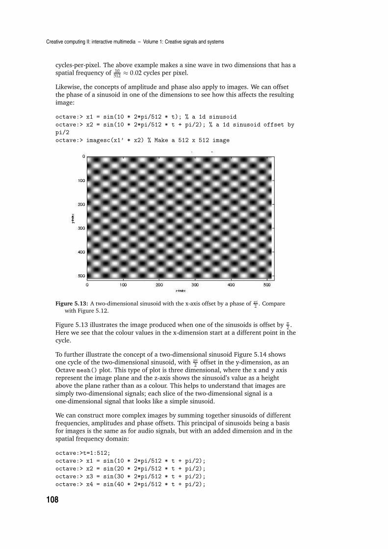
Creative computing II: interactive multimedia – Volume 1: Creative signals and systems
cycles-per-pixel. The above example makes a sine wave in two dimensions that has aspatial frequency of 10
512≈ 0.02 cycles per pixel.
Likewise, the concepts of amplitude and phase also apply to images. We can offsetthe phase of a sinusoid in one of the dimensions to see how this affects the resulting
image:
octave:> x1 = sin(10 * 2*pi/512 * t); % a 1d sinusoid
octave:> x2 = sin(10 * 2*pi/512 * t + pi/2); % a 1d sinusoid offset by
pi/2
octave:> imagesc(x1’ * x2) % Make a 512 x 512 image
Figure 5.13: A two-dimensional sinusoid with the x-axis offset by a phase of pi
2. Compare
with Figure 5.12.
Figure 5.13 illustrates the image produced when one of the sinusoids is offset by π2.
Here we see that the colour values in the x-dimension start at a different point in thecycle.
To further illustrate the concept of a two-dimensional sinusoid Figure 5.14 showsone cycle of the two-dimensional sinusoid, with pi
2offset in the y-dimension, as an
Octave mesh() plot. This type of plot is three dimensional, where the x and y axis
represent the image plane and the z-axis shows the sinusoid’s value as a heightabove the plane rather than as a colour. This helps to understand that images are
simply two-dimensional signals; each slice of the two-dimensional signal is a
one-dimensional signal that looks like a simple sinusoid.
We can construct more complex images by summing together sinusoids of different
frequencies, amplitudes and phase offsets. This principal of sinusoids being a basisfor images is the same as for audio signals, but with an added dimension and in the
spatial frequency domain:
octave:>t=1:512;
octave:> x1 = sin(10 * 2*pi/512 * t + pi/2);
octave:> x2 = sin(20 * 2*pi/512 * t + pi/2);
octave:> x3 = sin(30 * 2*pi/512 * t + pi/2);
octave:> x4 = sin(40 * 2*pi/512 * t + pi/2);
108

Image filtering
Mesh plot of one cycle of a 2d sinewave with pi/2 offset in y
1020
3040
50
x-index1020
3040
50
y-index
-1
-0.5
0
0.5
1
Colour value (amplitude)
Figure 5.14: A three-dimensional mesh plot of one cycle of the two-dimensional sinusoid of
Figure 5.13. The value of the sinusoidal function at each position index (x,y) is
represented as a height instead of as a colour.
octave:> x5 = sin(50 * 2*pi/512 * t + pi/2);
octave:> X = [x1;x2;x3;x4;x5]’ * [x1;x2;x3;x4;x5];
octave:> imagesc(X)
The above example shows the construction of a matrix from five sinusoids with
spatial frequencies being successive integer multiples of 10512
cycles per pixel, all with
phases offset by pi2
. The resulting image produced by imagesc() is shown in
Figure 5.15. This is a harmonic series of two-dimensional sinusoids, because theyhave frequency relationships that are successive integer multiples of a common
fundamental frequency. Is there a visible relationship between adding
two-dimensional sinusoids in the spatial domain and adding one-dimensionalsinusoids?
To assist in the analysis of two-dimensional signals use Octave’s mesh() plotfunction. However, it is important not to pass it too many values because the plot
will take a very long time to display. Figure 5.16 is a mesh plot of one cycle of thesignal shown in Figure 5.15. Here we can see that the construction of a harmonic
series of two-dimensional sinusoids constructs a periodic pulse with fundamental
spatial frequency 10512
cycles per pixel.
109
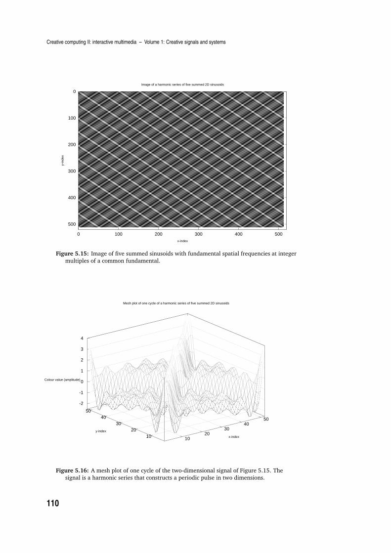
Creative computing II: interactive multimedia – Volume 1: Creative signals and systems
y-in
dex
x-index
Image of a harmonic series of five summed 2D sinusoids
0
100
200
300
400
500
0 100 200 300 400 500
Figure 5.15: Image of five summed sinusoids with fundamental spatial frequencies at integer
multiples of a common fundamental.
Mesh plot of one cycle of a harmonic series of five summed 2D sinusoids
1020
3040
50
x-index1020
3040
50
y-index
-2
-1
0
1
2
3
4
Colour value (amplitude)
Figure 5.16: A mesh plot of one cycle of the two-dimensional signal of Figure 5.15. The
signal is a harmonic series that constructs a periodic pulse in two dimensions.
110

Image filtering
Learning activity
Construct 512× 512 pixel images from each of the following mathematical expressions:
sum of ten 2D sinusoids with frequencies at integer multiples of a common fundamental of 1512cycles
per pixel
sum of ten 2D sinusoids with frequencies at integer multiples of a common fundamental of 1512cycles
per pixel and alternating phases of 0 and pi/2
vector product of two sinusoids – one with spatial frequency 1512cycles per pixel and the other with
spatial frequency 20512cycles per pixel.
Plot your results using both imagesc() and plot a 50× 50 region of each image using the mesh()function. [Hint: to plot the first 50× 50 patch of an image matrixX use mesh(X(1:50,1:50))].
Natural images
So far we have constructed and inspected synthetic images using mathematicalfunctions; this process is called image synthesis. Many images that we encounter in
creative practice are obtained by digitally sampling a photographic image.
The process for sampling a photographic image is similar to that of sampling an
audio signal, except that the sampling occurs in the spatial domain and in twodimensions.
We start with an image resolution which is the sampling rate in the x and ydimensions expressed in pixels per inch, or pixels per centimeter. It is common to
use a resolution of 200 pixels per inch in both the X and Y dimensions. Some digital
sampling systems use higher or lower resolutions than this; you will need to consultthe equipment user documentation to find the resolution of your equipment.
Assuming that an image has been saved in a digital format, such as JPEG, TIFF, GIFor PNG, we can load it into Octave using the imread() function. (Note: you should
find your own image with which to try out these examples. When we refer to‘carousel.jpg’, you should substitute the name of the image you are using for these
examples.)
octave:>A = imread(’/home/cc227/carousel.jpg’);
octave:>size(A)
ans =
933 705 3
Here, the image information is read from a JPEG format image file into a matrix thathas x and y dimensions of 933× 705; the size of the image in pixels. Each value in
the matrix is a number in the range [0..255] representing the brightness on an 8-bitscale. However, notice that there is another dimension to the image: the three colour
channels holding separate images for Red, Green and Blue. These are represented by
three two-dimensional matrix structures accessed inside the three dimensionalmatrix A. The individual colour-channel images can be extracted using: red =
A(:,:,1), green = A(:,:,2) and blue = A(:,:,3).
111
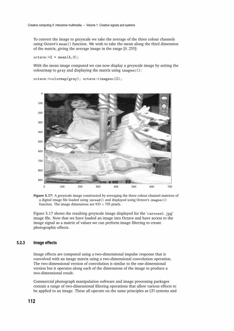
Creative computing II: interactive multimedia – Volume 1: Creative signals and systems
To convert the image to greyscale we take the average of the three colour channelsusing Octave’s mean() function. We wish to take the mean along the third dimension
of the matrix, giving the average image in the range [0..255]:
octave:>Z = mean(A,3);
With the mean image computed we can now display a greyscale image by setting the
colourmap to gray and displaying the matrix using imagesc():
octave:>colormap(gray); octave:>imagesc(Z);
0
100
200
300
400
500
600
700
800
900
0 100 200 300 400 500 600 700
Figure 5.17: A greyscale image constructed by averaging the three colour-channel matrices of
a digital image file loaded using imread() and displayed using Octave’s imagesc()
function. The image dimensions are 933× 705 pixels.
Figure 5.17 shows the resulting greyscale image displayed for the ‘carousel.jpg’
image file. Now that we have loaded an image into Octave and have access to theimage signal as a matrix of values we can perform image filtering to create
photographic effects.
5.2.3 Image effects
Image effects are computed using a two-dimensional impulse response that is
convolved with an image matrix using a two-dimensional convolution operation.
The two-dimensional version of convolution is similar to the one-dimensionalversion but it operates along each of the dimensions of the image to produce a
two-dimensional result.
Commercial photograph manipulation software and image processing packages
contain a range of two-dimensional filtering operations that allow various effects tobe applied to an image. These all operate on the same principles as LTI systems and
112

Image filtering
linear filtering as described above and in the last chapter.
To see how this works, we use the Octave function conv2() which takes two
matrices as arguments. The first argument is the image matrix and the second is theimpulse response. As noted in the last chapter, the order of the signals does not
affect the result. The following sections explore different two-dimensional impulseresponses and the effect of convolution of an image on each of them.
Image shift
Recall that a delayed impulse convolved with a one-dimensional signal causes the
signal to be delayed in time. We can translate an image to a different location byconvolving it with a two-dimensional impulse that is shifted in x and y relative to an
origin. A two-dimensional impulse response is often called a kernel in image
processing literature; the kernel is usually symmetric and consists of an odd-numberof samples. Common examples are 3× 3, 5× 5 and 25× 25. The centre-point of the
kernel is taken as the origin, so the unit impulse is taken to be a square matrix with
the centre pixel set to 1 and the other pixels set to zero.
To construct a two-dimensional impulse we start by constructing a one dimensionalimpulse and use vector multiplication to make the two-dimensional kernel:
octave:>imp1 = [1 zeros(1,10)] % 11-point impulse
imp1 =
1 0 0 0 0 0 0 0 0 0 0
octave:>imp1 = shift(imp1,5) % shift by floor(11/2)=5 samples
imp1 =
0 0 0 0 0 1 0 0 0 0 0
octave:> kern1 = imp1’*imp1 % Use vector multiplication to make 2D
kernel
kern1 =
0 0 0 0 0 0 0 0 0 0 0
0 0 0 0 0 0 0 0 0 0 0
0 0 0 0 0 0 0 0 0 0 0
0 0 0 0 0 0 0 0 0 0 0
0 0 0 0 0 0 0 0 0 0 0
0 0 0 0 0 1 0 0 0 0 0
0 0 0 0 0 0 0 0 0 0 0
0 0 0 0 0 0 0 0 0 0 0
0 0 0 0 0 0 0 0 0 0 0
0 0 0 0 0 0 0 0 0 0 0
0 0 0 0 0 0 0 0 0 0 0
A call to the function conv2() with an image, Z from above, a kernel, kern1, and a
third argument same, yields the identity:
Z2 = conv2(Z,kern1,’same’); % ’same’ means centre the kernel
The ‘same’ argument tells conv2() to treat the centre point as the zero index. Points
that are to the left of, or above, the centre point are taken as negative shift values
and points that are to the right and below are positive shift values.
In this example we got the same set of values back in the output matrix after
convolution as those in the input matrix. We can verify this by subtracting the result
113

Creative computing II: interactive multimedia – Volume 1: Creative signals and systems
from the original image and summing over both dimensions:
sum(sum(Z2 - Z))
ans = 0
This confirms that the output image is exactly the same as the input image eventhough we have performed a convolution. Thus the kernel, kern1, is the identity
transform (i.e. the unit impulse or delta function).
We can now move the image to a different location in x and y by offsetting the
impulse relative to its zero-index. The following example constructs a shift of 256
pixels in x and 0 pixels in y using a 513 x 513 kernel:
octave:>kern2 = zeros(513,513); % Make an all-zeros kernel
octave:>kern2(256+257,257)=1; % centre is (257,257) so add 256 in x
octave:>Z2=conv2(Z,kern2,’same’); % perform the convolution
octave:>imagesc(Z2) % display the result
Figure 5.18 shows the result of the convolution. Compare with Figure 5.17. The
convolution takes much longer in this example than in the previous one. This isbecause the operation is equivalent to performing a one-dimensional convolution on
every row and column of the image with every row and column of the kernel
respectively. This takes significantly many more multiplications and additions thanfor the comparable one-dimensional case.
0
100
200
300
400
500
600
700
800
900
0 100 200 300 400 500 600 700
Figure 5.18: The result of convolving the photo in Figure 5.17 with a two-dimensional shift
kernel. The kernel shifts the image 256 pixels in x and 0 pixels in y.
As we learned in the last chapter, we can speed up the process of convolution bytransforming our signals to the frequency domain and using complex multiplication.
We can perform the same sequence of operations as the convolution with kern2
above using the two-dimensional Fourier transform in Octave:
114

Image filtering
octave:> % Take the 2D Fourier transform of the image Z
octave:> % Allow room in the transform for the convolution
octave:> size(Z)
ans =
933 705 % use these values and the 513 x 513 kernel to
octave:> % calculate FFT size
octave:> FZ = fft2(Z, 933+512, 705+512); % 2nd and 3rd arguments are
octave:> % size of Fourier transform
octave:> kern2 = zeros(513,513);
octave:> kern2(257+256,257)=1 % Construct a 2D ’shift’ (delay) kernel
octave:> % We must transpose the kernel when taking its Fourier transform
octave:> FK = fft2(kern2’, 933+512, 705+512); % 2D Fourier transform of kernel
octave:> FY = FZ.*FK’; % Convolution is element-wise complex multiplication
octave:> % notice that the convolution kernel Fourier transform is transposed
octave:> X = real(ifft2(FY)); % convolved image is inverse Fourier transform
octave:> % The FFT does not have the ’same’ argument, so we need to
octave:> % crop the resulting image
octave:> X = X(257:end-255, 257:end-255); % Crop extra pixels from start
octave:> % and end of each dimension
octave:> imagesc(X) % display the image
You should verify that the above recipe using the two-dimensional Fourier transform
produces the same result as the conv2() method. Can you think of a way to do this?
Learning activity
What happens when you omit the ‘same’ argument in conv2() in the kern2 convolution example
above? Why?
How can this be ‘fixed’ after convolution?
Perform each of the following shift operations on the ‘carousel.jpg’ image using either conv2() or
fft2(): [Hint: it will be a lot faster if you use fft2(); how much faster?]
100 pixels to the left
100 pixels to the left and 50 pixels up
256 pixels right and 0 pixels in y
256 pixels right and 256 pixels down.
Image echo
The basic operation of 2D image filtering can be used to perform numerous image
processing effects. The following example illustrates how to construct a kernel tomake image echoes consisting of layered, shifted versions of an image.
We use the same Fourier-transform convolution technique from above but we do notcrop the resulting image to be the ‘same’ size as the original. Instead, we keep the
full transform to allow the image to spread out to a larger canvas:
octave:> kern3=zeros(513,513); % Make a new empty kernel
115

Creative computing II: interactive multimedia – Volume 1: Creative signals and systems
octave:> % construct 5 echoes using a for loop
octave:> for k = 1:5
octave:> kern3(ceil(rand(1)*513),ceil(rand(1)*513))=0.2;
octave:> end
octave:> FK = fft2(kern3’, 933+512, 705+512);
octave:> FY = FZ.*FK;
octave:> X = real(ifft2(FY));
octave:> imagesc(X)
0
200
400
600
800
1000
1200
1400
0 200 400 600 800 1000 1200
Figure 5.19: The result of convolving the photo in Figure 5.17 with a two-dimensional echo
kernel. Here the kernel contains five randomly placed echoes that shift the image both in x
and y.
The result of this convolution is shown in Figure 5.19. The effect is to produceechoes of the original image but to make them brighter where they overlap more
and darker where the image is not overlapped with echoes.
Learning activity
Make echo kernels that have the following characteristics and test your kernels using frequency-domain
convolution:
three evenly-spaced echoes in the x-dimension only
three randomly-spaced echoes in the y-dimension only
five random echoes in x and y with random heights (impulse amplitudes).
116

Image filtering
Gaussian blur
octave:> n = 25; w = 0.25; % Gaussian size and dispersion params
octave:> g = exp(-0.5*(([0:n-1]’-(n-1)/2)*w).2̂); % Gaussian function
octave:> size(g)
ans =
25 1 octave:> % We use vector multiplication to make a 2D function
octave:> GaussKern = g * g’ ; % make two-dimensional Gaussian
octave:> % The kernel size minus 1 is 24, this is the ‘extra’ we need
octave:> FZ = fft2(Z, 933+24, 705+24);
octave:> FK = fft2(GaussKern’, 933+24, 705+24);
octave:> FY = FZ .* FK;
octave:> X = real(ifft2(FY));
octave:> imagesc(X(13:end-11,13:end-11)) % crop 12 pixels each side of
image
Figure 5.20 shows a mesh plot of the two-dimensional Gaussian kernel of length 25pixels. Figure 5.21 shows the result of convolving the image from Figure 5.17 with
the Gaussian kernel. This blurring effect is often used to ‘soften’ photographic
images in digital image manipulation software.
Two dimensional Gaussian kernel
510
1520
25
5
10
15
20
250
0.2
0.4
0.6
0.8
1
Figure 5.20: The two-dimensional Gaussian kernel is a bell curve, when convolved with an
image this produces a blurring effect.
Motion blur
Another blur effect is obtained if the blurring is restricted to one direction. This is
motion blur, it simulates the effect obtained when a fast-moving object is
photographed using a relatively slow shutter speed on a camera. The direction of theblur can be controlled by the orientation of the line of non-zero values in the kernel.
117
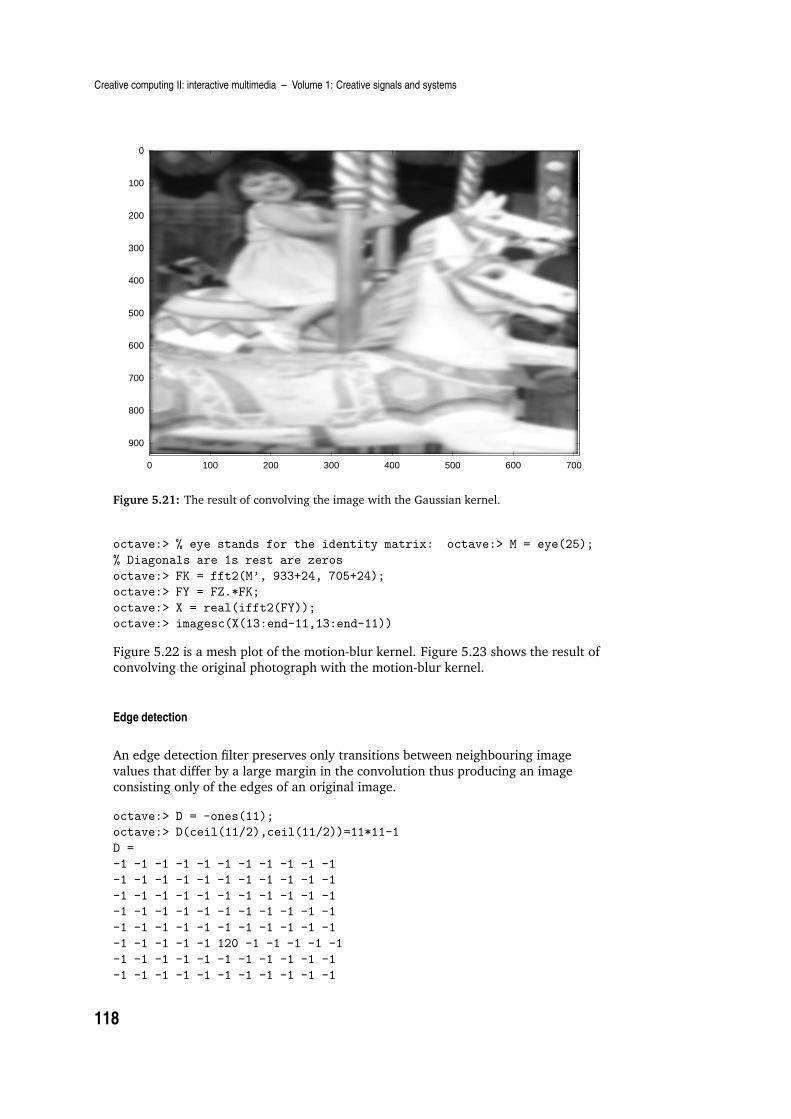
Creative computing II: interactive multimedia – Volume 1: Creative signals and systems
0
100
200
300
400
500
600
700
800
900
0 100 200 300 400 500 600 700
Figure 5.21: The result of convolving the image with the Gaussian kernel.
octave:> % eye stands for the identity matrix: octave:> M = eye(25);
% Diagonals are 1s rest are zeros
octave:> FK = fft2(M’, 933+24, 705+24);
octave:> FY = FZ.*FK;
octave:> X = real(ifft2(FY));
octave:> imagesc(X(13:end-11,13:end-11))
Figure 5.22 is a mesh plot of the motion-blur kernel. Figure 5.23 shows the result ofconvolving the original photograph with the motion-blur kernel.
Edge detection
An edge detection filter preserves only transitions between neighbouring image
values that differ by a large margin in the convolution thus producing an imageconsisting only of the edges of an original image.
octave:> D = -ones(11);
octave:> D(ceil(11/2),ceil(11/2))=11*11-1
D =
-1 -1 -1 -1 -1 -1 -1 -1 -1 -1 -1
-1 -1 -1 -1 -1 -1 -1 -1 -1 -1 -1
-1 -1 -1 -1 -1 -1 -1 -1 -1 -1 -1
-1 -1 -1 -1 -1 -1 -1 -1 -1 -1 -1
-1 -1 -1 -1 -1 -1 -1 -1 -1 -1 -1
-1 -1 -1 -1 -1 120 -1 -1 -1 -1 -1
-1 -1 -1 -1 -1 -1 -1 -1 -1 -1 -1
-1 -1 -1 -1 -1 -1 -1 -1 -1 -1 -1
118

Image filtering
Motion-blur kernel
510
1520
25
5
10
15
20
250
0.2
0.4
0.6
0.8
1
Figure 5.22: The motion-blur kernel is a line oriented in the direction of motion; when
convolved with an image this produces a direction blurring effect.
0
100
200
300
400
500
600
700
800
900
0 100 200 300 400 500 600 700
Figure 5.23: The result of convolving the image with the motion-blur kernel.
119

Creative computing II: interactive multimedia – Volume 1: Creative signals and systems
-1 -1 -1 -1 -1 -1 -1 -1 -1 -1 -1
-1 -1 -1 -1 -1 -1 -1 -1 -1 -1 -1
-1 -1 -1 -1 -1 -1 -1 -1 -1 -1 -1
octave:> sum(sum(D))
ans = 0
octave:> FZ = fft2(Z, 933+10, 705+10);
octave:> FK = fft2(D’, 933+10, 705+10);
octave:> FY = FZ.*FK;
octave:> X = real(ifft2(FY));
octave:> imagesc(X)
0
100
200
300
400
500
600
700
800
900
0 100 200 300 400 500 600 700
Figure 5.24: Convolution with edge-detecting kernel.
Low-pass filter
Constructing filters by hand is very difficult and often non-intuitive. Fortunately,
there exist functions that assist in digital filter design. For example, the fir1()
function used above for one-dimensional audio filtering can also be used to
construct a two-dimensional filter kernel.
We start by constructing a one-dimensional filter, as above, and we extend it to two
dimensions using vector multiplication. The cutoff frequency is expressed in
normalised frequency units as a fraction of π radians; in the case of images, thisfrequency is a spatial frequency in cycles per pixel.
The following Octave example illustrates how to make a low-pass filter kernel andapply it to an image:
octave:> f=fir1(512,.03);
octave:> F = f * f’;
120

Image filtering
octave:> FK = fft2(F’, 933+511, 705+511);
octave:> FY = FZ.*FK;
octave:> X = real(ifft2(FY));
octave:> X=X(257:end-255,257:end-255);
octave:> imagesc(X)
The result of the low-pass filter operation is shown in Figure 5.25. Note that the
low-pass filter operation is similar to the Gaussian blur filter that we used above.The input image has all the edge detail removed.
0
100
200
300
400
500
600
700
800
900
0 100 200 300 400 500 600 700
Figure 5.25: Convolution with a 512× 512 low-pass filter kernel with cutoff frequency 0.03π.
High-pass filter
The following example shows how to perform the same processing steps but to
create a high-pass filter:
octave:> f=fir1(512,.03,’high’);
octave:> F = f * f’;
octave:> FK = fft2(F’, 933+511, 705+511);
octave:> FY = FZ.*FK;
octave:> X = real(ifft2(FY));
octave:> X=X(257:end-255,257:end-255);
octave:> imagesc(X)
The resulting image is shown in Figure 5.26. A high-pass filter emphasizes the places
in the image where the colour values transition between contrasting values. The
effect is to emphasise the edges in the image, so the high-pass filter can be used asan edge-detector.
121
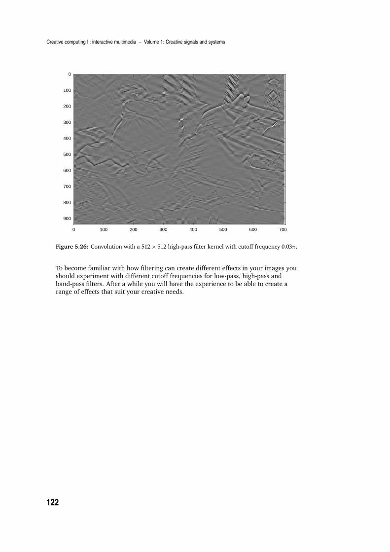
Creative computing II: interactive multimedia – Volume 1: Creative signals and systems
0
100
200
300
400
500
600
700
800
900
0 100 200 300 400 500 600 700
Figure 5.26: Convolution with a 512× 512 high-pass filter kernel with cutoff frequency 0.03π.
To become familiar with how filtering can create different effects in your images you
should experiment with different cutoff frequencies for low-pass, high-pass and
band-pass filters. After a while you will have the experience to be able to create arange of effects that suit your creative needs.
122

Summary and learning outcomes
Learning activity
All of the convolution operations in the above examples were performed in the frequency domain. The
following activity collects all the different transforms into a single function that you can use for all your image
filtering needs.
Write an Octave function called convImage() that takes three arguments: an image matrix, a 2D
convolution kernel and a third argument indicating whether to make the output image the ‘same’ size
as the input image.
Your function should take the two-dimensional Fourier transform of the image matrix and the
convolution kernel. The size dimensions of the Fourier transform should be the dimensions of the
image matrix plus the length of one side of the kernel minus 1: rows(X)+rows(H)-1,
columns(X)+columns(H)-1. The Fourier transform of the convolution kernel should transpose
the kernel.
The convolution itself is an element-wise matrix multiplication between the two complex Fourier
transformed matrices.
If the ‘same’ flag is present (test using if nargin == 3) then the output matrix should be cropped
so that the output image is the same size as the input image. The cropping should be symmetrical so
that the same number of pixels are removed from the top and bottom and left and right of the output
image.
For hints on how to perform these operations, study all of the examples above.
Make kernels for each of the following transforms and convolve your own image files using your
convImage() function:
a low-pass filter with cutoff 0.05π
a high-pass filter with cutoff 0.05π
an edge-detection filter with dimension 7× 7a Gaussian blur filter with dimension 5× 5.
5.3 Summary and learning outcomes
The fields of digital audio processing and digital image processing are vast. This
chapter has scratched the surface but you now have enough technical knowledge toexplore the subject further by reading textbooks, Internet sites and by exploring
freely-available software. You can investigate other kernels for audio and image
filtering by experimenting with digital audio and image processing packages such asAudacity, Photoshop and its free cousin The Gimp.
In many of these packages it is possible to extract the digital filter kernels bysupplying the software with a single impulse in the middle of an otherwise zero
audio or image signal. The resulting impulse response is the basis for your ownversion of the digital filter.
This technique only works if the filter being analysed is an LTI system. While manydigital audio and image processing packages are based on LTI systems theory, not all
of them are, so your analyses may vary in success from one application to another.
123

Creative computing II: interactive multimedia – Volume 1: Creative signals and systems
The most important aspect of LTI systems that we have investigated is that a vastcollection of applications and transformations can be reduced to a single operation:
convolution. It is vital to understand how to use convolution as a first step to moreadvanced methods that you may encounter.
With a knowledge of the contents of this chapter and its directed reading andactivities, you should be able to:
discuss the relationship between signal processing, and audio and visual effects
describe and implement a range of audio effects
describe and implement a range of image filtering effects.
5.4 Exercises
In addition to the exercises listed below, you should attempt all of the learningactivities throughout this chapter, to enhance your understanding of the material.
1. What is a room response? What are some of the practical reasons for finding out
what a room response is?
What is meant by early and late response? Why would it be useful to know whatthe early response is? Why would it be useful to know what the late response is?
How is a room response determined?
2. Can you think of a visual analogue to the concept of a room response? Explainand discuss your answer.
3. All of the image processing examples in Section 5.2.3 above transformed a
greyscale image. To work in colour we must transform the individual colour
channels. Load a colour image from your collection and work through thefollowing:
Make a red-only image by copying the matrix returned by imread() andzeroing the green and blue colour planes. [Hint: the Octave operator
A(:,:,1) accesses colour plane 1 in the three-dimensional matrix
representation used by Octave for colour images.]
Perform a low-pass, high-pass and band-pass convolution on each of the
three colour channels separately. Display your colour filtering operations
using octave’s imshow() function.
Combine your three transformed colour channels into a single
three-dimensional matrix. Display the result using the imshow() function.
124