creating a new model to predict cooling tower performance
TRANSCRIPT

University of Massachusetts Amherst University of Massachusetts Amherst
ScholarWorks@UMass Amherst ScholarWorks@UMass Amherst
Masters Theses Dissertations and Theses
July 2015
Creating a New Model to Predict Cooling Tower Performance and Creating a New Model to Predict Cooling Tower Performance and
Determining Energy Saving Opportunities through Economizer Determining Energy Saving Opportunities through Economizer
Operation Operation
Pranav Yedatore Venkatesh University of Massachusetts Amherst
Follow this and additional works at: https://scholarworks.umass.edu/masters_theses_2
Part of the Engineering Commons
Recommended Citation Recommended Citation Yedatore Venkatesh, Pranav, "Creating a New Model to Predict Cooling Tower Performance and Determining Energy Saving Opportunities through Economizer Operation" (2015). Masters Theses. 489. https://doi.org/10.7275/7073706 https://scholarworks.umass.edu/masters_theses_2/489
This Open Access Thesis is brought to you for free and open access by the Dissertations and Theses at ScholarWorks@UMass Amherst. It has been accepted for inclusion in Masters Theses by an authorized administrator of ScholarWorks@UMass Amherst. For more information, please contact [email protected].

CREATING A NEW MODELTO PREDICT COOLING TOWER
PERFORMANCE AND DETERMINING ENERGY SAVING
OPPORTUNITIES THROUGH ECONOMIZER OPERATION
A Thesis Presented
by
PRANAV YEDATORE VENKATESH
Submitted to the Graduate School of the
University of Massachusetts Amherst in partial fulfillment
of the requirements for the degree of
MASTER OF SCIENCE
May 2015
Mechanical and Industrial Engineering

© Copyright by Pranav Yedatore Venkatesh 2015
All Rights Reserved

CREATING A NEW MODEL TO PREDICT COOLING TOWER
PERFORMANCE AND DETERMINING ENERGY SAVING
OPPORTUNITIES THROUGH ECONOMIZER OPERATION
A Thesis Presented
by
PRANAV YEDATORE VENKATESH
Approved as to style and content by:
______________________________
Dragoljub Kosanovic, Chair
______________________________
Jon McGowan, Member
______________________________
Stephen Nonnenmann, Member
__________________________________
Donald Fisher, Department Head
Department of Mechanical & Industrial Engineering

iv
ACKNOWLEDGEMENTS
First and foremost I would like to express my sincere gratitude to my advisor,
Prof. Dragoljub Kosanovic, for giving me an opportunity to work with him when I first
arrived at the University of Massachusetts Amherst. His constant encouragement,
guidance and support during the course of my study have allowed me to learn a lot.
I would like to thank Prof. Jon McGowan for his expert advice, interesting
courses and agreeing to serve on my thesis committee. I would like to thank Prof.
Stephen Nonnenmann for agreeing to serve on my thesis committee.
I would also like to thank my co-workers, Benjamin McDaniel, Bradley Newell,
Hariharan Gopalakrishnan, Ghanshyam Gaudani, Justin Marmaras, Alex Quintal and
Jorge Soares, at the Industrial Assessment Center for providing feedback and making this
learning experience fruitful.
Last but not the least, I would like to thank my parents for their constant support
and faith in me.

v
ABSTRACT
CREATING A NEW MODEL TO PREDICT COOLING TOWER PERFORMANCE
AND DETERMINING ENERGY SAVING OPPORTUNITIES THROUGH
ECONOMIZER OPERATION
MAY 2015
PRANAV YEDATORE VENKATESH, B.E., VISVESVARAYA TECHNOLOGICAL
UNIVERSITY, INDIA
M.S., UNIVERSITY OF MASSACHUSETTS AT AMHERST
Directed by: Dr. Dragoljub Kosanovic
Cooling towers form an important part of chilled water systems and perform the
function of rejecting the heat to the atmosphere. Chilled water systems are observed to
constitute a major portion of energy consumption in air conditioning systems of
commercial buildings and of process cooling in manufacturing plants. It is frequently
observed that these systems are not operated optimally, and cooling towers being an
integral part of this system present a significant area to study and determine possible
energy saving measures. More specifically, operation of cooling towers in economizer
mode in winter (in areas where winter temperatures drop to 40°F and below) and variable
frequency drives (VFDs) on cooling tower fans [1] are measures that can provide
considerable savings. The chilled water system analysis tool (CWSAT) software is
developed as a primary screening tool for energy evaluation for chilled water systems.
This tool quantifies the energy usage of the various chilled water systems and typical
measures that can be applied to these systems to conserve energy. The tool requires

vi
minimum number of inputs to analyze the component-wise energy consumption and
incurred overall cost. The current cooling tower model used in CWSAT was developed
by Benton [2]. A careful investigation of the current model indicates that the prediction
capability of the model at lower wet bulb temperatures (close to 40°F and below) and at
low fan power is not very accurate. This could be a result of the lack of data at these
situations when building the model. A new model for tower performance prediction is
imperative since economizer operation occurs at low temperatures and most cooling
towers come equipped with VFDs. In this thesis, a new model to predict cooling tower
performance is created to give a more accurate picture of the various energy conservation
measures that are available for cooling towers. The weaknesses of the current model are
demonstrated and prediction capabilities of the new model analyzed and validated.
Further the economic feasibility of having additional cooling tower capacity to allow for
economizer cooling, in light of reduced tower capacity at lower temperatures [3] is
investigated.

vii
TABLE OF CONTENTS
Page
ACKNOWLEDGEMENTS ............................................................................................... iv
ABSTRACT ........................................................................................................................ v
LIST OF TABLES ............................................................................................................. ix
LIST OF FIGURES ........................................................................................................... xi
NOMENCLATURE ........................................................................................................ xiv
CHAPTER
1. INTRODUCTION ........................................................................................................ 1
1.1 Cooling Towers ................................................................................................. 1
1.2 Cooling Tower Classification ........................................................................... 4
1.3 Literature Review............................................................................................ 11
1.4 Research Objectives ........................................................................................ 15
1.5 Organization .................................................................................................... 16
2. EXISTING MODELS AND THEIR LIMITATIONS ............................................... 17
2.1 Drawbacks of Thermodynamic Models .......................................................... 17
2.2 Limitations of Existing Model ........................................................................ 21
3. COOLING TOWER PERFORMANCE DATA COLLECTION............................... 28
3.1 Data Collection Source ................................................................................... 28
3.2 Data Collection Approach............................................................................... 29
4. NEW MODEL CREATION ....................................................................................... 35
4.1 Model Creation Techniques ............................................................................ 35
4.2 New Model Creation through Polynomial Regression ................................... 39
4.3 New Model Creation through Artificial Neural Networks ............................. 53
4.4 Comparison of Techniques ............................................................................. 58

viii
5. WATER SIDE ECONOMIZER / FREE COOLING ................................................. 60
5.1 Reduction in Cooling Tower Capacity at Low Temperatures ........................ 60
5.2 Comparison of Prediction Capability of the different Models........................ 64
5.3 Benefits of Larger Cooling Tower Capacity to meet Winter Load ................ 70
6. CONCLUSIONS......................................................................................................... 75
5.1 Summary ......................................................................................................... 75
5.2 Recommendations for Future Work................................................................ 76
APPENDICES
A. SAMPLE TOWER PERFORMANCE GRAPH ........................................................ 78
B. MATLAB CODE USED FOR TOWER PERFORMANCE PREDICTION ............. 79
REFERENCES ................................................................................................................. 89

ix
LIST OF TABLES
Table Page
3.1: Extent of Cooling Tower Selection Software Parameter Variation ........................ 29
3.2: Tower Manufacturer A Performance across Various Tonnages for a
CF tower .................................................................................................................. 31
3.3: Tower Manufacturer B Performance across Various Tonnages for a
CF tower .................................................................................................................. 32
3.4: Tower Manufacturer A Performance across Various Tonnages for a
XF tower .................................................................................................................. 33
3.5: Tower Manufacturer B Performance across Various Tonnages for a
XF tower .................................................................................................................. 34
4.1: Regression Coefficients over the six folds and average for Counterflow
Tower ...................................................................................................................... 42
4.2: Regression Coefficients over the six folds and average for Crossflow
Tower ...................................................................................................................... 43
4.3: Comparison of the Old and New Models for a Counter Flow Tower ..................... 46
4.4: Comparison of the Old and New Models for a Cross Flow Tower ......................... 46
5.1: Conditions of Air entering and leaving the Cooling Tower .................................... 62
5.2: ARI Loading Schedule ............................................................................................ 65
5.3: Parameters considered to simulate tower performance ........................................... 65
5.4: Comparison of Tower Energy Prediction across models and CWSAT for a
Tower with ARI Loading schedule ......................................................................... 66
5.5: Comparison of energy savings predicted thorough the models and CWSAT for a
Tower with ARI Loading Schedule ........................................................................ 67
5.6: Comparison of energy savings predicted thorough the models and CWSAT for a
Tower with Process Loading ................................................................................... 67
5.7: Comparison of free cooling hours predicted thorough the models and CWSAT ... 67
5.8: Predicted Cost Savings associated with VSD and Free Cooling ............................ 68
5.9: Increase in Chiller Energy Savings with additional Tower for ARI
loading schedule ...................................................................................................... 71

x
5.10: Increase in Chiller Energy Savings with additional Tower for a constant
process load ............................................................................................................. 72
5.11: Economic Benefit of an additional cooling tower ................................................... 72
xi
LIST OF FIGURES
Figure Page
1.1: Schematic of a Typical Mechanical Draft Cooling tower ......................................... 2
1.2: Classification of Cooling Towers .............................................................................. 5
1.3: Triangular Slat Splash Fill ......................................................................................... 7
1.4: Typical Film fill for a Cooling Tower ....................................................................... 8
1.5: Schematic of Forced Draft and Induced Draft Cooling Towers ............................. 10
1.6: Schematic of Crossflow and Counterflow Cooling Towers .................................... 11
1.7: Summary of models available for analyzing wet cooling towers ........................... 13
2.1: Error in Tower Performance Prediction with at 73% Fan Power ........................... 24
2.2: Error in Tower Performance Prediction with at 51% Fan Power ........................... 25
2.3: Error in Tower Performance Prediction with at 34% Fan Power ........................... 25
2.4: Error in Tower Performance Prediction with at 22% Fan Power ........................... 26
2.5: Variation in Tower Performance with wet bulb temperature for a Counter
Flow Tower ............................................................................................................. 26
2.6: Variation in Tower Performance with wet bulb temperature for a Cross
Flow Tower ............................................................................................................. 27
4.1: Basic Structure of an Artificial Neuron ................................................................... 38
4.2: Two Layer Feed Forward Neural Network Architecture ........................................ 38
4.3: Statistical results of Regression over one of the folds ............................................ 41
4.4: Actual Approach vs Predicted Approach of the Old Model for a CF Tower .......... 44
4.5: Actual Approach vs Predicted Approach of the New Model for a CF Tower ........ 44
4.6: Actual Approach vs Predicted Approach of the Old Model for a XF Tower ......... 45
4.7: Actual Approach vs Predicted Approach of the New Model for a XF Tower ........ 45
4.8: Comparison of Error between the old and new model at Range=15°F for a
Counter Flow Tower ............................................................................................... 47

xii
4.9: Comparison of Error between the old and new model at Range=15°F for a
Counter Flow Tower ............................................................................................... 47
4.10: Comparison of Error between the old and new model at Range=10°F for a
Counter Flow Tower ............................................................................................... 48
4.11: Comparison of Error between the old and new model at Range=10°F for a
Counter Flow Tower ............................................................................................... 48
4.12: Comparison of Error between the old and new model at Range=5°F for a
Counter Flow Tower ............................................................................................... 49
4.13: Comparison of Error between the old and new model at Range=5°F for a
Counter Flow Tower ............................................................................................... 49
4.14: Comparison of Error between the old and new model at Range=15°F for a
Cross Flow Tower ................................................................................................... 50
4.15: Comparison of Error between the old and new model at Range=15°F for a
Cross Flow Tower ................................................................................................... 50
4.16: Comparison of Error between the old and new model at Range=10°F for a
Cross Flow Tower ................................................................................................... 51
4.17: Comparison of Error between the old and new model at Range=10°F for a
Cross Flow Tower ................................................................................................... 51
4.18: Comparison of Error between the old and new model at Range=5°F for a
Cross Flow Tower ................................................................................................... 52
4.19: Comparison of Error between the old and new model at Range=5°F for a
Cross Flow Tower ................................................................................................... 52
4.20: Error Histogram for Neural Network Fitting with One Hidden layer of
Neurons ................................................................................................................... 54
4.21: Performance for Neural Network Fitting with One Hidden layer of Neurons ........ 54
4.22: Regression Plots for Neural Network Fitting with One Hidden layer of
Neurons ................................................................................................................... 55
4.23: Error Histogram for Neural Network Fitting with Two Hidden layers of
Neurons ................................................................................................................... 56
4.24: Performance for Neural Network Fitting with Two Hidden layers of Neurons ...... 56
4.25: Regression Plots for Neural Network Fitting with Two Hidden layers of
Neurons ................................................................................................................... 57
xiii
5.1: Conditions of Air Entering and Leaving the tower on a Psychrometric Chart ....... 62
5.2: Variation in Tower Capacity with Wet Bulb Temperature ..................................... 63
5.3: Variation in Tower Fan Power with Load and Wet Bulb Temperature
as predicted by CWSAT ........................................................................................ 69
5.4: Variation in Tower Fan Power with Load and Wet Bulb Temperature
as predicted by the Old Model ................................................................................ 70
5.5: Variation in Tower Fan Power with Load and Wet Bulb Temperature
as predicted by the New Model ............................................................................... 70
5.2: Tower Performance Variation with Fan Speeed ..................................................... 74
5.3: VSD Efficiencies at varying Motor Speeds ............................................................ 74

xiv
NOMENCLATURE
ANN Artificial Neural Network
ARI Air-Conditioning & Refrigeration Institute
CF Counter Flow
CHWST CHilled Water Setpoint Temperature
CT Cooling Tower
CTI Cooling Tower Institute
CWSAT Chilled Water System Assessment Tool
CWT Condenser Water Temperature
EWT Entering Water Temperature
GPM Gallons Per Minute
HVAC Heating Ventilation and Air Conditioning
LWT Leaving Water Temperature
PR Polynomial Regression
VFD Variable Frequency Drive
VSD Variable Speed Drive
XF Cross Flow

1
CHAPTER 1
INTRODUCTION
1.1 Cooling Towers
A cooling tower is a device that is used to cool a water stream while
simultaneously rejecting heat to the atmosphere. In systems involving heat transfer, a
condenser is a device that is used to condense the fluid flowing through it from a gaseous
state to a liquid state by cooling the fluid. This cooling to the fluid flowing through a
condenser, is generally provided by a cooling tower. Cooling towers may also be used to
cool fluids used in a manufacturing process. As a result we see that cooling towers are
commonly used in
1. HVAC (Heating Ventilation and Air-Conditioning) to reject the heat from chillers
2. Manufacturing to provide process cooling
3. Electric power generation plants to provide cooling for the condenser
Cooling tower operation is based on evaporative cooling as well as exchange of
sensible heat. During evaporative cooling in a cooling tower, a small quantity of the
water that is being cooled is evaporated in a moving stream of air to cool the rest of the
water. Also when warm water comes in contact with cooler air, there is sensible heat
transfer whereby the water is cooled. The major quantity heat transfer to the air is through
evaporative cooling while only about 25% of the heat transfer is through sensible heat.
Figure 1.1 taken from Mulyandasari [4] shows the schematic of a cooling tower.

2
Figure 1.1 Schematic of a Typical Mechanical Draft Cooling tower
Some important terms relating to cooling towers as described by Stanford [5] are:
Approach- It is the difference between the temperature of water leaving the
cooling tower and the wet bulb temperature. It is used as an indicator of how close
to wet bulb temperature the water exiting the tower is.
Range- It is the difference between the temperature of water entering the tower
and temperature of water leaving the tower.
Capacity- The total amount of heat a cooling tower can reject at a given flow rate,
approach and wet bulb temperature. It is generally measured in tons.
Cell- It is the smallest tower subdivision that can operate independently. Each
individual cell of a tower can have different water flow rate and air flow rate.
Fill- The heat transfer media or surface designed to maximize the air and water
surface contact area.

3
Make up water- The additional water that needs to be added to offset water lost to
evaporation, drift, blowdown and other losses.
Dry bulb temperature – It is the temperature of air measured by a thermometer
freely exposed to the air but shielded from moisture and radiation. In general
when temperature is referred to, it is dry bulb temperature.
Wet bulb temperature – It is the temperature of air measured by a thermometer
whose bulb is moistened and exposed to air flow. It can also be said to be the
adiabatic saturation temperature. The wet bulb temperature is always lesser than
the dry bulb temperature other than the condition of 100% relative humidity when
the two temperatures are equal.
Free Cooling or Waterside Economizer Operation – It is the operation of the
cooling tower in conditions where just the cooling tower is able to provide the
required temperature cold water for HVAC or process needs without needing
mechanical cooling from the chiller. This saves energy because while the chiller
may utilize about 0.7 kW/ton, the tower is now able to provide the same cooling
at about 0.2 kW/ton.
According to Hill [6] the factors influencing the performance of a cooling tower are:
1. The cooling range
2. The approach
3. The ambient wet bulb temperature
4. The flow rate of water through the tower
5. The flow rate of air over the water
6. The ambient temperature

4
7. The type of fill in the tower
8. Total surface area of contact between water and air
1.2 Cooling Tower Classification
Cooling towers can be classified in many different ways as follows
Classification by build
Package type
Field Erected type
Classification based on heat transfer method
Wet cooling tower
Dry Cooling tower
Fluid Cooler
Classification based on type of Fill
Spray Fill
Splash Fill
Film Fill
Classification based on air draft
Atmospheric tower
Natural Draft Tower
Mechanical Draft Tower
Forced Draft

5
Induced Draft
Classification based on air flow pattern
Crossflow
Counterflow
Figure 1.2 shows the graphical depiction of the tower classification.
Figure 1.2 Classification of Cooling Towers
Classification by build
Package type cooling towers are preassembled and can be easily transported and
erected at the location of use. These are generally suitable for applications where the heat
load to be rejected is not very large (most HVAC and process load applications).
Field erected type of towers are usually much larger to handle the larger heat
rejection loads and are custom built as per customer requirements. Most of the
Cooling Towers
Classification based on Build
Package type
Field Erected type
Classification based on Heat
Transfer Method
Wet Cooling Tower
Dry Cooling Tower
Fluid Cooler
Classification based on Type
of Fill
Spray Fill
Splash Fill
Film Fill
Classification based on Air
Draft
Atmospheric Tower
Natural Draft Tower
Mechanical Draft Tower
Forced Draft
Induced Draft
Classification based on Air Flow Pattern
Crossflow Tower
CounterFlow Tower

6
construction /assembly of the tower takes place at the site where the tower will be
located.
This thesis will be to build a model that predicts the performance of package type
towers. Although the performance of field erected type towers may be similar to package
type towers, the predicted performance may not be very accurate as a result of the unique
and requirement specific construction of field erected type towers.
Classification based on heat transfer method
Wet cooling towers are the most common type of cooling towers and the ones
referred to when talking about cooling towers. As explained earlier, they operate on the
principle of evaporative cooling. The water to be cooled and the ambient air come in
direct contact with each other. This thesis will look mainly at the performance prediction
of wet cooling towers since they are the most widely used.
In a dry cooling tower there is a surface (e.g. tube of a heat exchanger) that
separates the water from the ambient air. There is no evaporative cooling in this case.
Such a tower may be used when the fluid to be cooled needs to be protected from the
environment.
In a fluid cooler water is sprayed over tubes through which the fluid to be cooled
is flowing while a fan may also be utilized to provide a draft. This incorporates the
mechanics of evaporative cooling in a wet cooling tower while also allowing the working
fluid to be free of contaminants or environmental contact.
Classification based on type of Fill
In a spray fill tower the water is broken down into small droplets so that the area
of contact between the water surface and air is increased. So in a way spray fill is not
7
really a fill because there is no packing in the tower. Small droplets of water are created
by spraying through nozzles, which are contained within the tower casing, through which
there is airflow. The drawbacks of this kind of a fill are low efficiency, large tower size
and large airflow requirement.
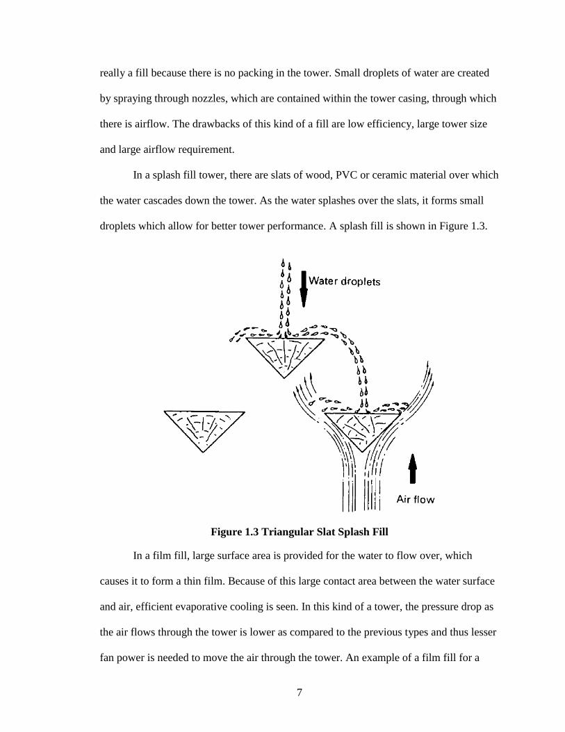
In a splash fill tower, there are slats of wood, PVC or ceramic material over which
the water cascades down the tower. As the water splashes over the slats, it forms small
droplets which allow for better tower performance. A splash fill is shown in Figure 1.3.
Figure 1.3 Triangular Slat Splash Fill
In a film fill, large surface area is provided for the water to flow over, which
causes it to form a thin film. Because of this large contact area between the water surface
and air, efficient evaporative cooling is seen. In this kind of a tower, the pressure drop as
the air flows through the tower is lower as compared to the previous types and thus lesser
fan power is needed to move the air through the tower. An example of a film fill for a

8
cooling tower is shown in Figure 1.4. Film fill is less expensive and more efficient than
splash fill and has resulted in its widespread use in cooling towers.
Figure 1.4 Typical Film fill for a Cooling Tower
Classification based on air draft
In an atmospheric tower the air enters the tower through louvers driven by its own
velocity. This kind of a tower is inexpensive. Since the performance is greatly affected by
wind conditions it is largely inefficient and is seldom used when accurate and consistent
cold water temperatures are required.

9
A natural draft tower (also known as hyperbolic cooling tower) is similar to an
atmospheric tower in that there is no mechanical device to create air flow through the
tower. However it is dependable and consistent unlike an atmospheric tower. The air flow
through the tower is a result of the density differential between hot and less dense air
inside the tower as compared to the relatively cooler and denser ambient air outside the
tower. The hot air rises up through the tower while cool ambient air is drawn in through
inlets at the bottom of the tower. Natural draft towers are extensively used in electric
power generation plants and areas where there is higher relative humidity. These towers
are much more expensive as compared to other tower types and conspicuous by their
hyperbolic shape which is so designed because
The natural upward draft is enhanced by such a shape
This shape provides better structural strength and stability
Sometimes natural draft towers are equipped with fans to augment the air flow
and are referred to as fan assisted natural draft towers or hybrid draft towers.
Mechanical draft towers have one or more fans that are used to move the air
through the tower to provide predictable and consistent performance making them the
tower of choice in most HVAC and process applications. A mechanical draft tower can
be subdivided in two types, namely, forced draft towers and induced draft towers.
The tower is termed a forced draft tower if the fans are arranged so as to blow air
into the tower. Thus there is a positive pressure in the tower fill as compared to the
outside. In this case the fans are generally located at the point where the air enters the
tower.

10
The tower is termed an induced draft tower if the fans are arranged so as to push
air out of the tower. Thus there is a negative pressure in the tower fill as compared to
outside. The fan is located at the point where the air leaves the tower.
Figure 1.5 shows the configuration of the cooling tower for forced draft and
induced draft fans as taken from Stanford [5].
Figure 1.5 Schematic of Forced Draft and Induced Draft Cooling Towers
11
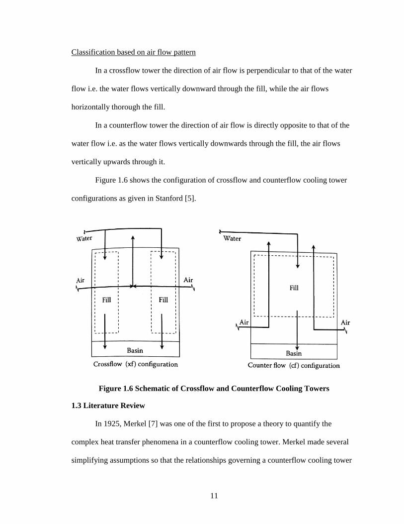
Classification based on air flow pattern
In a crossflow tower the direction of air flow is perpendicular to that of the water
flow i.e. the water flows vertically downward through the fill, while the air flows
horizontally thorough the fill.
In a counterflow tower the direction of air flow is directly opposite to that of the
water flow i.e. as the water flows vertically downwards through the fill, the air flows
vertically upwards through it.
Figure 1.6 shows the configuration of crossflow and counterflow cooling tower
configurations as given in Stanford [5].
Figure 1.6 Schematic of Crossflow and Counterflow Cooling Towers
1.3 Literature Review
In 1925, Merkel [7] was one of the first to propose a theory to quantify the
complex heat transfer phenomena in a counterflow cooling tower. Merkel made several
simplifying assumptions so that the relationships governing a counterflow cooling tower

12
could be solved much more easily. Benton [2] and Kloppers and Kroger [8] list the
assumptions of the Merkel theory as follows
The saturated air film is at the temperature of bulk water
The saturated air film offers no resistance to heat transfer
The vapor content of the air is proportional to the partial pressure of water vapor
The force driving heat transfer is the differential enthalpy between saturated and
bulk air
The specific heat of the air water vapor mixture and heat of vaporization are
constant.
The loss of water by evaporation is neglected. (This simplification has a greater
influence at elevated ambient temperatures)
The air exiting the tower is saturated with water vapor and is characterized only by
its enthalpy. (This assumption regarding saturation has a negligible influence
above ambient temp of 68°F but is of importance at lower temperatures)
The Lewis factor relating heat and mass transfer is equal to 1. (This assumption
has a small influence but affects results at low temperatures.)
This model has been widely applied because of its simplicity. Baker and Shryock
[9] give a detailed explanation of the procedure of arriving at the final equations of the
Merkel theory and also list some of the shortcomings of the Merkel theory and suggest
some corrections. Bourillot [10] developed a program called TEFERI to predict the
performance of an evaporative cooling tower in 1983. Benton [11] developed the FACTS
model in 1983 and compared it to test data. Benton [2] states that the FACTS model is
widely used by the utilities to model cooling tower performance. Majumdar [12]
13
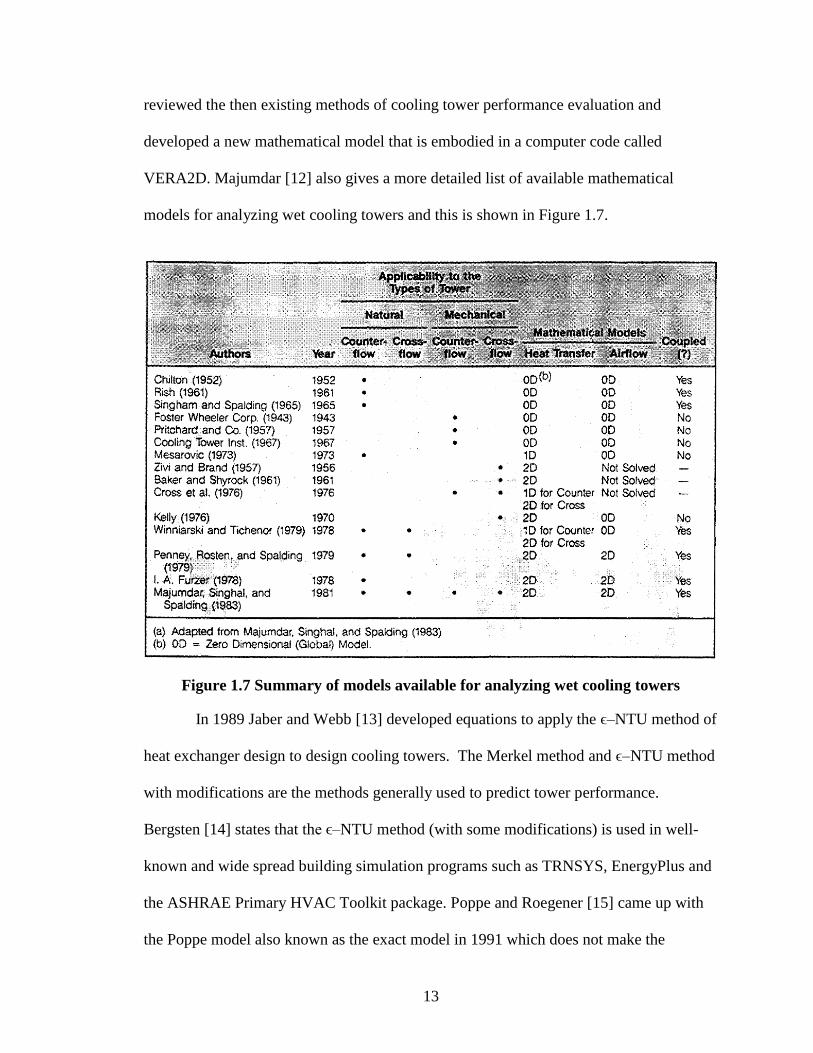
reviewed the then existing methods of cooling tower performance evaluation and
developed a new mathematical model that is embodied in a computer code called
VERA2D. Majumdar [12] also gives a more detailed list of available mathematical
models for analyzing wet cooling towers and this is shown in Figure 1.7.
Figure 1.7 Summary of models available for analyzing wet cooling towers
In 1989 Jaber and Webb [13] developed equations to apply the ϵ–NTU method of
heat exchanger design to design cooling towers. The Merkel method and ϵ–NTU method
with modifications are the methods generally used to predict tower performance.
Bergsten [14] states that the ϵ–NTU method (with some modifications) is used in well-
known and wide spread building simulation programs such as TRNSYS, EnergyPlus and
the ASHRAE Primary HVAC Toolkit package. Poppe and Roegener [15] came up with
the Poppe model also known as the exact model in 1991 which does not make the

14
simplifying assumptions of Merkel’s theory and is therefore more accurate. Kloppers and
Kroeger [16] critically evaluate the Merkel theory by comparing it with the Poppe
method. Kloppers and Kroger [8] give a detailed derivation of the Merkel, Poppe and
Entu methods, their comparison and how to solve the governing equations in each of the
methods. They conclude that the Poppe method is more accurate than the Merkel and ϵ–
NTU methods and that the Merkel and ϵ–NTU methods give identical results since they
are based on the same simplifying assumptions. With the advancement of computing
power, computational Fluid Dynamics (CFD) models have been created to simulate
performance of cooling towers [17].
Ebrahim et al [18] looked at the thermal performance of cooling towers under
variable wet bulb temperature and report that as the wet bulb temperature increases, the
approach, range and evaporation loss all increase considerably. Other information about
low temperature tower performance is hard to come by.
The DOE-2, a widely used building energy analysis program predicts the cooling
tower performance through a statistical model. Benton et al [2] say that the DOE2 uses a
12 parameter variable curve fit. They further develop a statistical model through multiple
linear least squares regression of vendor data and compare it to the DOE2 model, Merkel
model, ϵ–NTU model and Poppe model. They surmise that the statistically developed
model is comparable to the analytically developed ones and is better than the DOE2
model while also being faster than the other models.
To conclude, all the past literature have served as driving factors for this research
and show that there has been an effort to predict performance of cooling towers. The
literature review also reveals that none of the models have been created for a regular user
15
(e.g. a chilled water system operator) to be able to determine possible energy saving
opportunities. All the aforestated models require a lot of computation and significant
knowledge of the tower type, structure, materials used and thermodynamic properties.
Further they do not give much information about cooling tower operation at low
temperatures or about economizer operation of the cooling tower (also known as free
cooling). Creating a new model to study cooling tower performance through a wider
range of temperatures while also trying to keep the required parameters to a minimum
without sacrificing accuracy will go a long way towards realizing opportunities for
energy savings
1.4 Research Objectives
The objective is to create a new model to predict cooling tower performance over
a larger operating range thereby allowing for better determination of energy saving
measures like free cooling and VFDs on cooling tower fans. This will need to be carried
out without making the process cumbersome so that an average user would be able to use
the model, to achieve fairly accurate results without the model demanding too many
inputs. Towards this objective, the following steps were carried out:
1) Collect a large range of cooling tower operating data from cooling tower
manufacturers that is suitable to analyze the extent of validity of the current
model as well as create a new model to simulate cooling tower performance
2) Compare the existing model in CWSAT to manufacturer tower data to identify
and quantify the shortcomings of the current model
3) Create a new model and validate the results
4) Compare the new model with the existing model to demonstrate improvements

16
5) Demonstrate that the cooling tower performance reduces when operated in free
cooling mode at lower wet bulb temperatures
6) Determine if installing oversized cooling towers is economically feasible to take
advantage of economizer operation
1.5 Organization
Chapter 1 gives an introduction. Chapter 2 starts off with a discussion on the
limitations of existing models as outlined in the literature review. Chapter 3 dives into the
how the data for creating a new model was collected and what the sources were. Chapter
4 gives a detailed account of methods available to create new models and the polynomial
regression method used to create a new model in this thesis. The model performance is
verified and the results discussed. Chapter 5 addresses the reduction of cooling tower
capacity when operated in a free cooling mode at low temperatures and the benefits of
having a larger tower capacity to be able to incorporate free cooling operation in winter
months. In Chapter 6 a summary is given and recommendations for future work are
made.

17
CHAPTER 2
EXISTING MODELS AND THEIR LIMITATIONS
The purpose of a cooling tower model is to be able to predict the cooling tower
performance. However not all models are suitable for an average user to utilize and
determine energy use and possible saving measures. This thesis and chapter focusses on
the existing models capability to meet the needs of a user to easily estimate cooling tower
energy use and look at possible energy savings.
2.1 Drawbacks of Thermodynamic Models
In the literature review it was observed that there were numerous models to
predict cooling tower performance through thermodynamics and heat transfer principles.
Before moving on to create a new model, a few of the drawbacks of such models will be
discussed.
Amongst the thermodynamic models found in literature, the simplest one was
seen to be the Merkel method. According to Kloppers [16], the Merkel equation is given
by
wi
wo
T
d fi fr fi d fi fi pw w
M
w w masw maT
h a A L h a L c dTMe
m G i i
(2.1)
Where,
MMe = Transfer coefficient or Merkel number
dh = Mass transfer coefficient, 2kg/m s
fia = Surface area of fill per unit volume of the fill, 1m

18
frA = Frontal Area; 2m
fiL = Length of fill; m
wm = Mass flow rate of water; kg/s
pwc = Specific heat of water at constant pressure; J/kgK
maswi = Enthalpy of mean air saturated with water; J/kg
mai = Enthalpy of mean air; J/kg
wiT = Temperature of water at inlet of the tower; K
woT = Temperature of water at outlet of the tower; K
Kloppers [16] also states that it is difficult to evaluate the surface area per unit
volume of fill due to the complex nature of the two phase flow in fills. However it is not
necessary to explicitly specify the surface area per unit volume or the mass transfer
coefficient since the value of the Merkel number can be obtained by integrating the right
hand side of the equation above. Further it is to be noted that the exact state of the air
leaving the fill cannot be calculated and is assumed to be saturated with water vapor so
that temperature of water leaving the fill may be calculated. Bourillot [10] has stated that
the Merkel method is simple to use and can correctly predict the cold water temperature
when an appropriate value of coefficient is used but is insufficient for estimating the
characteristics of warm air leaving the fill and for calculation of changes in the water
flow rate due to evaporation. Using the equation above requires quite a few parameters
that are not easily available to an average person and if we are looking at information on
how air flow rate will affect the temperature of water leaving the tower (to determine
19
savings possible through VFD operation of the tower fan) it is impossible to proceed
without having even more information.
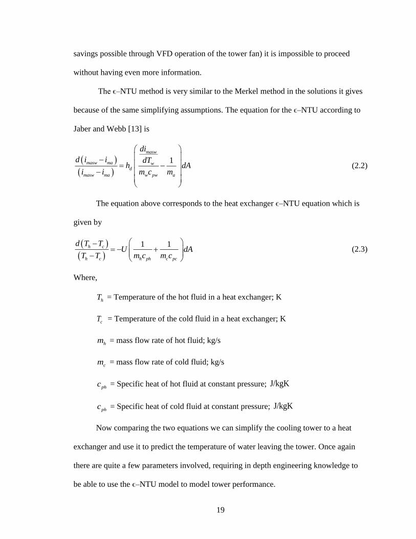
The ϵ–NTU method is very similar to the Merkel method in the solutions it gives
because of the same simplifying assumptions. The equation for the ϵ–NTU according to
Jaber and Webb [13] is
1
masw
masw ma wd
masw ma w pw a
di
d i i dTh dA
i i m c m
(2.2)
The equation above corresponds to the heat exchanger ϵ–NTU equation which is
given by
1 1h c
h c h ph c pc
d T TU dA
T T m c m c
(2.3)
Where,
hT = Temperature of the hot fluid in a heat exchanger; K
cT = Temperature of the cold fluid in a heat exchanger; K
hm = mass flow rate of hot fluid; kg/s
cm = mass flow rate of cold fluid; kg/s
phc = Specific heat of hot fluid at constant pressure; J/kgK
phc = Specific heat of cold fluid at constant pressure; J/kgK
Now comparing the two equations we can simplify the cooling tower to a heat
exchanger and use it to predict the temperature of water leaving the tower. Once again
there are quite a few parameters involved, requiring in depth engineering knowledge to
be able to use the ϵ–NTU model to model tower performance.

20
Next we look at the Poppe model. The governing equations for the heat and mass
transfer in the fill for unsaturated air are given by the following equations.
1
pwP
w masw ma f masw ma sw v sw pw w
cMe
dT i i Le i i w w i w w c T
(2.4)
a
w
P w
w sw
dwm
dTMe dT
m w w
(2.5)
0.667
0.6221
0.6220.865
0.622ln
0.622
sw
f
sw
w
wLe
w
w
(2.6)
1w wi ao
a a wi
m m mw w
m m m
(2.7)
Where,
PMe = Merkel number according to Poppe method
fLe = Dimensionless Lewis factor
w = Humidity Ratio of air; kg water vapor/ kg dry air
sww = Humidity Ratio of air saturated with water; kg water vapor/ kg dry air
ow = Humidity Ratio of air at outlet of tower; kg water vapor/ kg dry air
One method of solving these governing differential equations is by the fourth
order Runge-Kutta method according to Kloppers [8] and is clearly outlined in [8].
Further [8] says that the air outlet conditions can be calculated from the equations above
and that since the value of 0w is not known a priori, the equations are solved iteratively.
Kloppers [8] also says that the Poppe method predicts the water content of the exiting air
accurately and the results are consistent with full scale cooling tower test results.
21
Kloppers [16] concludes that if the temperature of water leaving the tower is of interest,
then both the Merkel and Poppe model predict identical temperatures. Further the Merkel
method predicts heat rejection rates and air outlet temperatures very accurately when the
actual outlet air is supersaturated with water vapor but when the ambient air is relatively
hot and dry, the outlet air may be unsaturated and the number predicted by the Poppe and
Merkel model may differ significantly. The Merkel and ϵ–NTU model give almost
identical answers because of the same underlying assumptions. The Poppe model gives
overall better results since no assumptions regarding the state of exiting air or Lewis
number are made but is comparatively more complex to solve than the Merkel method
whose assumptions make solving it a simpler hand calculation.
As discussed in the literature review earlier, there are many other models which
utilize similar equations based on thermodynamics to predict tower performance. Without
droning on further about how these models are unsuitable, it can be concluded that all
thermodynamic models require considerable information to be able to use them to predict
tower thermodynamic performance. The reason for this is that these models are not meant
for an average user to determine tower fan energy use but rather for tower designers in
building and evaluating towers who have all of the information readily at hand. Thus we
have a strong case for surrogate models which can do away with the unnecessary
thermodynamics and use information that is more readily available to predict tower
performance without losing accuracy.
2.2 Limitations of Existing Model
In the literature review it was identified that there are two metamodels, one is
used in the DOE2 engine and the other was developed by Benton et al. [2]. Information

22
about the model used in DOE2 was unavailable and [2] say that their model is more
accurate than the DOE2 model. A metamodel is an engineering method used when an
outcome of interest cannot be easily directly measured, so a model of the outcome is used
instead. The advantages of a metamodel are that it takes into account the variables that
affect the process and which are readily available to the user to use as predictors. Benton
[2] choose the parameters for their model as the wet bulb temperature, the range, water
flow, fan power and approach. These parameters represent the extent of the information
available to an average user and thus represent a very good set of parameters for a
surrogate model. These parameters are suitable because
a) Wet Bulb Temperature – For most locations, typical meteorological year (TMY)
data is available that can be used to determine the wet bulb temperature on an
hourly basis. Suitable sensors if present in the system can also obtain this
information.
b) Range – The cooling tower user will have the need to obtain a certain temperature
difference between the tower inlet and outlet.
c) Water flow – This information is also readily available to the user. If not directly
available, it can be measured relatively easily or even a value closely estimated.
d) Fan power – This is once again information that is readily known or that can be
measured.
e) Approach – A user would like to determine the approach based on previous four
parameters. Approach is the dependent variable while the remaining four are the
independent variables. This may be depicted in the form of an equation as follows
, , , wbApproach f T Range Water flow Fan Power
23
This metamodel is not only simple to use because of the easily available
information but also gives results comparable to thermodynamic models [2]. In this way a
surrogate model allows to predict the temperature of water leaving the cooling tower in a
much simpler manner, while also keeping it relevant with the available parameters. This
also allows us to incorporate the fan energy in the model more easily which is the
parameter of most importance to an average user. CWSAT current utilizes this model to
predict fan power usage.
As discussed earlier the opportunities for energy savings on a cooling tower are
through implementation of a VSD on the cooling tower fan [1] and operating the cooling
tower in free cooling mode [3, 5, 19]. There are also savings possible by changing the
temperature requirement of cold water required from the tower. For e.g. during free
cooling, the temperature of water from the tower required may not be as low as 45°F but
only 55°F since the 45°F requirement is mostly to maintain the required level of
humidity. Since the water content in the air is much lower in winter, the temperature of
cold water required may not be as low as 45°F, but rather 55°F. Increasing the cold water
temperature from the tower will decrease the fan energy usage as well as increase the
number of hours when free cooling is possible and therefore energy savings. Figure 5.2 in
Chapter 5 outlines the capacity of the tower at different values of cold water temperature.
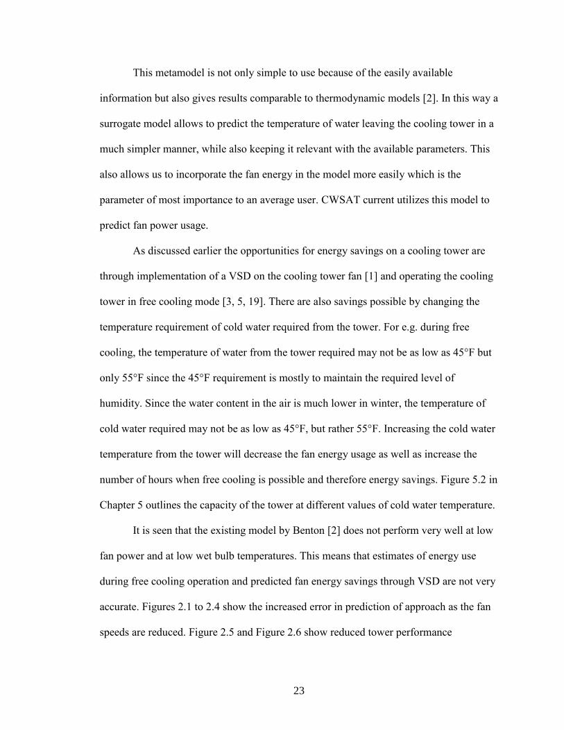
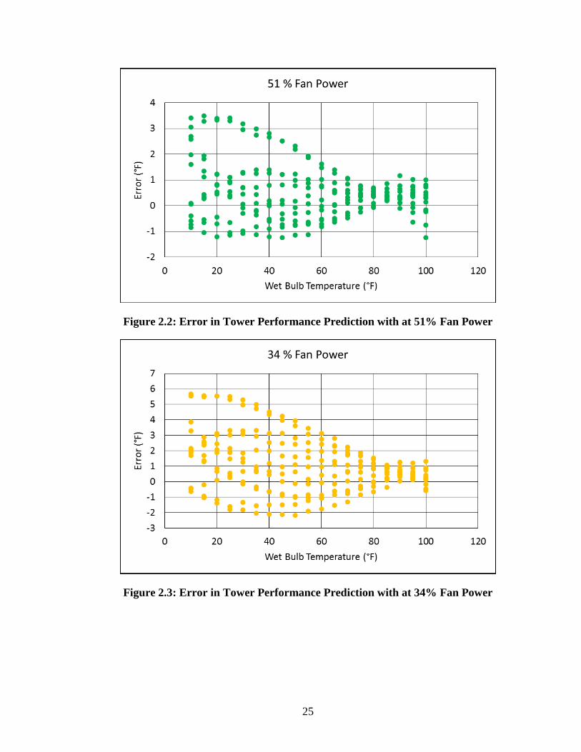
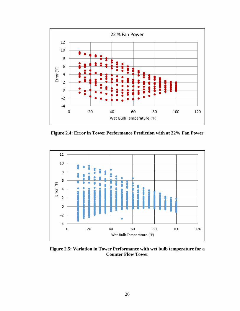
It is seen that the existing model by Benton [2] does not perform very well at low
fan power and at low wet bulb temperatures. This means that estimates of energy use
during free cooling operation and predicted fan energy savings through VSD are not very
accurate. Figures 2.1 to 2.4 show the increased error in prediction of approach as the fan
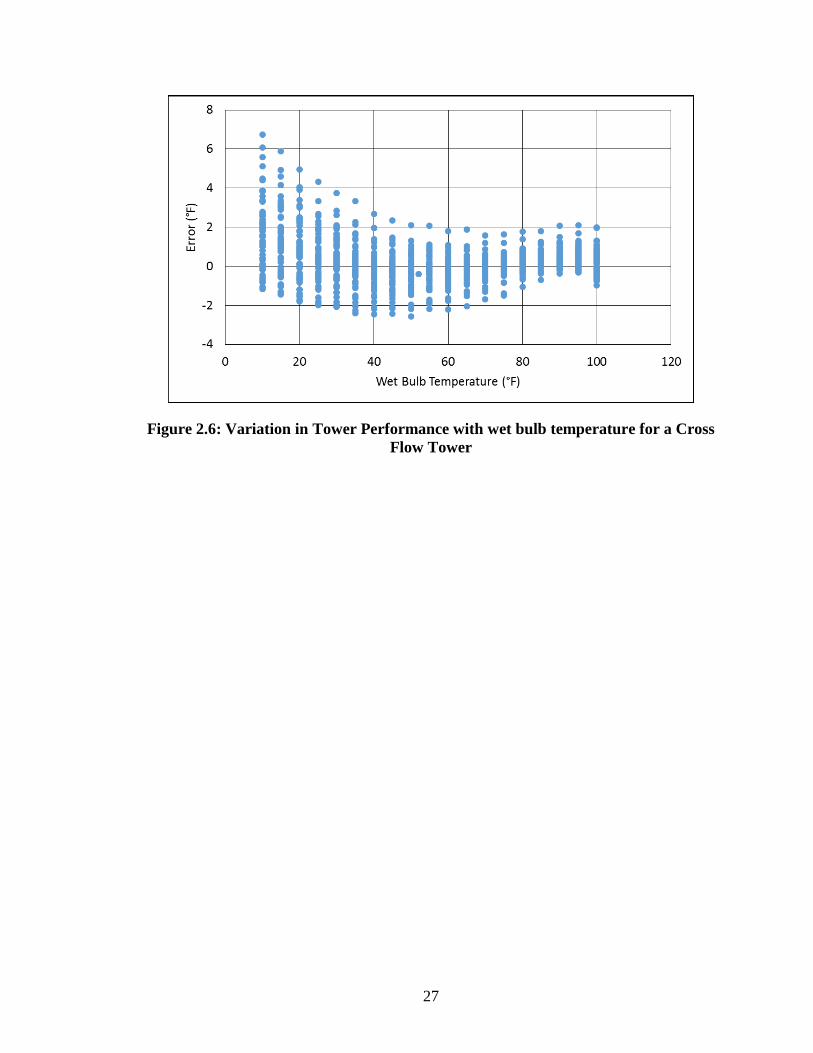
speeds are reduced. Figure 2.5 and Figure 2.6 show reduced tower performance

24
prediction capability at low wet bulb temperature for a counter flow tower. As the wet
bulb temperature reduces the magnitude of error is seen to increase. The lowering of
prediction capability at lower wet bulb temperature can also be seen in the Figures 2.1 to
2.4 for fan speed variation. This makes a strong case for creation of a new model that can
better predict cooling tower performance at these conditions.
Figure 2.1: Error in Tower Performance Prediction with at 73% Fan Power
25
Figure 2.2: Error in Tower Performance Prediction with at 51% Fan Power
Figure 2.3: Error in Tower Performance Prediction with at 34% Fan Power
26
Figure 2.4: Error in Tower Performance Prediction with at 22% Fan Power
Figure 2.5: Variation in Tower Performance with wet bulb temperature for a
Counter Flow Tower
27
Figure 2.6: Variation in Tower Performance with wet bulb temperature for a Cross
Flow Tower

28
CHAPTER 3
COOLING TOWER PERFORMANCE DATA COLLECTION
Cooling tower performance data is very difficult to access. Most cooling tower
manufacturers have proprietary software that they use when providing customers help in
selecting a tower. While the Cooling Tower Institute (CTI) certifies some cooling towers
sold by many manufacturers on thermal performance, they do not take into account the
tower performance in low temperature conditions. This chapter discusses the source and
method for data collection required for creating a new model.
3.1 Data Collection Source
The cooling tower data collected needs to be expansive and easy to collect. It was
found that Baltimore Aircoil Company (hereinafter referred to as Tower Manufacturer A)
and Marley Cooling Towers (hereinafter referred to as Tower Manufacturer B) have a
product selection software that generates graphs for the different conditions specified. A
graph digitizer was used to gather data points accurately from the graphs (a sample graph
is shown in Appendix A) for use in verifying the existing model and then creating a new
model.
It was seen that the Tower Manufacturer A was able to provide a larger variation
of parameters for wet bulb temperature and water flow as compared to Tower
Manufacturer B. Table 3.1 shows the range of variation of different parameters allowed
on both the selection software.
29
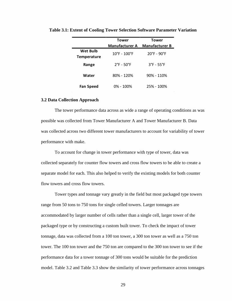
Table 3.1: Extent of Cooling Tower Selection Software Parameter Variation
3.2 Data Collection Approach
The tower performance data across as wide a range of operating conditions as was
possible was collected from Tower Manufacturer A and Tower Manufacturer B. Data
was collected across two different tower manufacturers to account for variability of tower
performance with make.
To account for change in tower performance with type of tower, data was
collected separately for counter flow towers and cross flow towers to be able to create a
separate model for each. This also helped to verify the existing models for both counter
flow towers and cross flow towers.
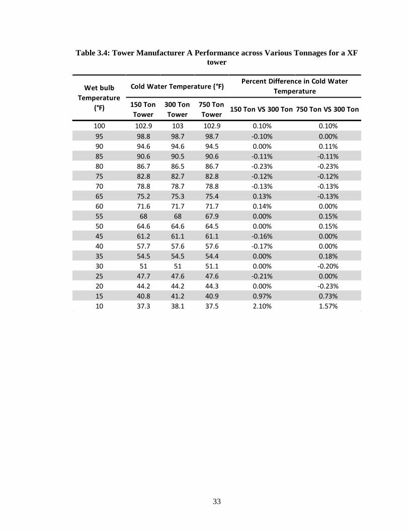
Tower types and tonnage vary greatly in the field but most packaged type towers
range from 50 tons to 750 tons for single celled towers. Larger tonnages are
accommodated by larger number of cells rather than a single cell, larger tower of the
packaged type or by constructing a custom built tower. To check the impact of tower
tonnage, data was collected from a 100 ton tower, a 300 ton tower as well as a 750 ton
tower. The 100 ton tower and the 750 ton are compared to the 300 ton tower to see if the
performance data for a tower tonnage of 300 tons would be suitable for the prediction
model. Table 3.2 and Table 3.3 show the similarity of tower performance across tonnages
Tower
Manufacturer A
Tower
Manufacturer BWet Bulb
Temperature10°F - 100°F 20°F - 90°F
Range 2°F - 50°F 3°F - 55°F
Water 80% - 120% 90% - 110%
Fan Speed 0% - 100% 25% - 100%

30
for counter flow towers for Tower Manufacturer A and Tower Manufacturer B
respectively. Table 3.4 and Table 3.5 show the similarity of tower performance across
tonnages for cross flow cooling towers for Tower Manufacturer A and Tower
Manufacturer B respectively. It is observed that a 300 ton tower is a good estimate for
tower performance since performance doesn’t vary more than a few percent points for
both the tower manufacturers across the range of tower tonnages. The water flow and fan
power is maintained a 100% across tonnages. The performance remains the same since
the cooling tower works on the principle of evaporative cooling where the water can be
cooled only as low as the wet bulb. Thus no matter the tonnage, since the water flow in
gpm/ton is constant and the fan speed is at a 100% the temperature of water leaving the
tower tends to be the same. This also saves time on collecting identical data for a large
number of tower tonnages for the same tower type.

31
Table 3.2: Tower Manufacturer A Performance across Various Tonnages for a CF
tower
100 Ton
Tower
300 Ton
Tower
750 Ton
Tower100 Ton VS 300 Ton 750 Ton VS 300 Ton
100 103.2 103 102.8 -0.19% 0.19%
95 98.7 98.9 98.6 0.20% 0.30%
90 94.6 94.6 94.3 0.00% 0.32%
85 90.6 90.4 90.5 -0.22% -0.11%
80 86.5 86.6 86.6 0.12% 0.00%
75 82.7 82.7 82.7 0.00% 0.00%
70 79 79 79.1 0.00% -0.13%
65 75.2 75.3 75.7 0.13% -0.53%
60 71.6 71.9 72.1 0.42% -0.28%
55 67.9 68.3 68.8 0.59% -0.73%
50 64.4 64.9 65.3 0.77% -0.62%
45 61.1 61.5 62.2 0.65% -1.14%
40 57.7 58.4 59 1.20% -1.03%
35 54.3 55.1 55.9 1.45% -1.45%
30 51 52 52.8 1.92% -1.54%
25 47.6 48.5 49.6 1.86% -2.27%
20 44 45.1 46.3 2.44% -2.66%
15 40.6 41.6 42.7 2.40% -2.64%
10 36.9 38.1 39 3.15% -2.36%
Wet bulb
Temperature
(°F)
Cold Water Temperature (°F)Percent Difference in Cold Water
Temperature

32
Table 3.3: Tower Manufacturer B Performance across Various Tonnages for a CF
tower
100 Ton
Tower
300 Ton
Tower
750 Ton
Tower100 Ton VS 300 Ton 750 Ton VS 300 Ton
100 102.3 102.6 102.5 0.29% 0.10%
95 98.4 98.2 98 -0.20% 0.20%
90 94.5 94.3 94.1 -0.21% 0.21%
85 90.5 90.5 90.4 0.00% 0.11%
80 86.6 86.5 86.4 -0.12% 0.12%
75 82.9 82.9 82.8 0.00% 0.12%
70 79.1 79.1 79.1 0.00% 0.00%
65 75.5 75.7 75.6 0.26% 0.13%
60 72 72.3 72.3 0.41% 0.00%
55 68.7 69.1 69 0.58% 0.14%
50 65.5 65.7 65.8 0.30% -0.15%
45 62.2 62.5 62.7 0.48% -0.32%
40 59 59.3 59.6 0.51% -0.51%
35 55.7 56.4 56.7 1.24% -0.53%
30 52.7 53 53.6 0.57% -1.13%
25 49.4 50.3 50.6 1.79% -0.60%
20 46.3 47.1 47.5 1.70% -0.85%
15 43.2 44 44.4 1.82% -0.91%
10 40 41 41.3 2.44% -0.73%
Wet bulb
Temperature
(°F)
Cold Water Temperature (°F)Percent Difference in Cold Water
Temperature
33
Table 3.4: Tower Manufacturer A Performance across Various Tonnages for a XF
tower
150 Ton
Tower
300 Ton
Tower
750 Ton
Tower150 Ton VS 300 Ton 750 Ton VS 300 Ton
100 102.9 103 102.9 0.10% 0.10%
95 98.8 98.7 98.7 -0.10% 0.00%
90 94.6 94.6 94.5 0.00% 0.11%
85 90.6 90.5 90.6 -0.11% -0.11%
80 86.7 86.5 86.7 -0.23% -0.23%
75 82.8 82.7 82.8 -0.12% -0.12%
70 78.8 78.7 78.8 -0.13% -0.13%
65 75.2 75.3 75.4 0.13% -0.13%
60 71.6 71.7 71.7 0.14% 0.00%
55 68 68 67.9 0.00% 0.15%
50 64.6 64.6 64.5 0.00% 0.15%
45 61.2 61.1 61.1 -0.16% 0.00%
40 57.7 57.6 57.6 -0.17% 0.00%
35 54.5 54.5 54.4 0.00% 0.18%
30 51 51 51.1 0.00% -0.20%
25 47.7 47.6 47.6 -0.21% 0.00%
20 44.2 44.2 44.3 0.00% -0.23%
15 40.8 41.2 40.9 0.97% 0.73%
10 37.3 38.1 37.5 2.10% 1.57%
Wet bulb
Temperature
(°F)
Cold Water Temperature (°F)Percent Difference in Cold Water
Temperature

34
Table 3.5: Tower Manufacturer B Performance across Various Tonnages for a XF
tower
In all, 1,350 data points were collected for both counter flow cooling towers and
cross flow cooling towers each. Of the 1,350 data points, 798 data points were obtained
from Tower Manufacturer A and 552 data points from Tower Manufacturer B. Each data
point corresponds to the approach of the tower based on the four parameters of wet bulb
temperature, range, percent water flow and percent fan power. Once all of the data is
collected, a new model is created as discussed in Chapter 4.
150 Ton
Tower
300 Ton
Tower
750 Ton
Tower150 Ton VS 300 Ton 750 Ton VS 300 Ton
100 102.3 102.6 102.5 0.29% 0.10%
95 98.4 98.2 98 -0.20% 0.20%
90 94.5 94.3 94.1 -0.21% 0.21%
85 90.5 90.5 90.4 0.00% 0.11%
80 86.6 86.5 86.4 -0.12% 0.12%
75 82.9 82.9 82.8 0.00% 0.12%
70 79.1 79.1 79.1 0.00% 0.00%
65 75.5 75.7 75.6 0.26% 0.13%
60 72 72.3 72.3 0.41% 0.00%
55 68.7 69.1 69 0.58% 0.14%
50 65.5 65.7 65.8 0.30% -0.15%
45 62.2 62.5 62.7 0.48% -0.32%
40 59 59.3 59.6 0.51% -0.51%
35 55.7 56.4 56.7 1.24% -0.53%
30 52.7 53 53.6 0.57% -1.13%
25 49.4 50.3 50.6 1.79% -0.60%
20 46.3 47.1 47.5 1.70% -0.85%
15 43.2 44 44.4 1.82% -0.91%
10 40 41 41.3 2.44% -0.73%
Wet bulb
Temperature
(°F)
Cold Water Temperature (°F)Percent Difference in Cold Water
Temperature

35
CHAPTER 4
NEW MODEL CREATION
This chapter deals with the creation of a new model for cooling tower
performance. Available techniques of surrogate model creation are investigated and the
method of polynomial regression is chosen as a suitable technique for this situation. All
the steps involved in the creation of a new model are discussed. The results are then
verified and improvements over the previous model are presented.
4.1 Model Creation Techniques
Forrester and Keane [20], Koziel et al. [21] and Queipo et.al. [22] give a detailed
account of the methods suitable for constructing surrogate models. The methods
generally used are
1. Polynomial Regression (PR)
2. Artificial Neural Networks (ANN)
3. Kriging
4. Radial Basis Functions (RBF)
5. Moving Least Squares (MLS)
6. Support Vector Regression (SVR)
Of these varied techniques, polynomial regression (PR) and artificial neural networks
(ANN) are discussed. The reason for choosing polynomial regression is that the current
model is based on polynomial regression and thus represents a good opportunity to create
a new model in the same manner and compare it with the older one. The reason for
choosing ANNs is that they represent a relatively new method of model creation and it
36
would be useful to determine if this method gives good solutions and see its advantages
and disadvantages as compared to polynomial regression.
Polynomial regression is a form of linear regression in which the relationship
between the independent variables and the dependent variables is modelled as an nth
degree polynomial. According to Queipo et.al. [22] Polynomial Regression (PR) is a
methodology that studies the quantitative association between a function of interest f ,
and PRGN basis functionsjz , where there are SN sample values of the function of interest
if , for a set of basis functions( )i
jz . For each observation i , a linear equation is formulated
as given below where the errors i are considered independents with expected value equal
to zero and variance 2 . The ̂ are the estimated parameters (by method of least squares)
are unbiased and have minimum variance.
( ) 2
1
z , 0 , PRGN
i
i j j i i i
j
f z E E V
(4.1)
The same can be represented in a much simpler fashion as follows
2f X , 0, =E V I (4.2)
Where X is a S PRGN N matrix of basis functions with the design variables for sampled
points.
For this specific case of modelling approach as a function of four design variables
1 2 3 4, , and x x x x i.e. wet bulb temperature, range, percent water flow and percent fan
power respectively, the complete equation for the model will yield 35 terms and is
represented as follows,

37
0 1 1 2 2 3 3 4 4
2 2 2 2
5 1 6 2 7 3 8 4
9 1 2 10 1 3 11 1 4 12 2 3 13 2 4 14 3 4
3 3 3 3
15 1 16 2 17 3 18 4
Approach x x x x
x x x x
x x x x x x x x x x x x
x x x x
19 1 2 3 20 1 3 4 21 1 2 4 22 2 3 4
2 2 2
23 1 2 24 1 3 25 1 4
2 2 2
26 2 1 27 2 3 28 2 4
2 2 2
29 3 1 30 3 2 31 3 4
2
32 4 1 33
x x x x x x x x x x x x
x x x x x x
x x x x x x
x x x x x x
x x
2 2
4 2 34 4 3x x x x
(4.3)
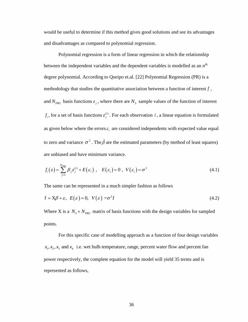
Artificial Neural Networks (also referred to as just neural networks) are
computational models that are inspired by biological nervous systems and consist of
neurons that perform operations. Koziel et.al. [21] state that the neuron performs an
affine transformation followed by a nonlinear operation. If the inputs to a neuron are
denoted as 1 2, , , nx x x , then the neuron output is computed as
1
1 T
y
e
(4.4)
Where 1 1 n nw x w x , with 1 2, , , nw w w being regression coefficients,
being the bias value of a neuron and T being the user defined slope or parameter. This is
depicted in Figure 4.1 taken from Gershenson [23]. The equation 4.4 above is a sigmoid
activation function. The other commonly used activation functions are the threshold and
hyperbolic tangent. The sigmoid function is preferred in this case since it represents a
smooth, continuous, nonlinear function. The most common neural network architecture is
the multi-layer feed-forward network and is shown in Figure 4.2. Once a suitable network
architecture is chosen, the next step is to train the ANN. The inputs and their
corresponding outputs are given to the ANN which “learns” and adjusts the weights to be
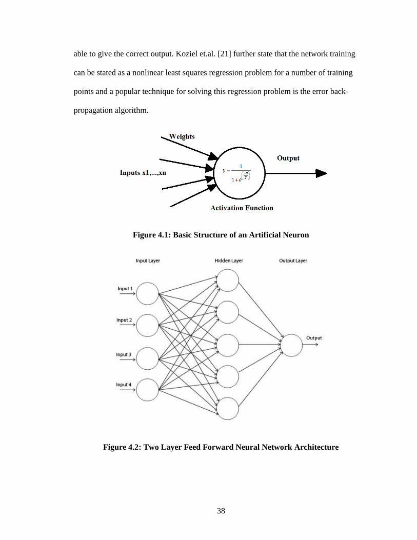
38
able to give the correct output. Koziel et.al. [21] further state that the network training
can be stated as a nonlinear least squares regression problem for a number of training
points and a popular technique for solving this regression problem is the error back-
propagation algorithm.
Figure 4.1: Basic Structure of an Artificial Neuron
Figure 4.2: Two Layer Feed Forward Neural Network Architecture

39
4.2 New Model Creation through Polynomial Regression
The data collection process has been discussed. Also as discussed earlier, the
new model is a third order polynomial regression with the approach as the dependent
variable and wet bulb temperature, range, water flow and fan power as the independent
variables. Before starting on the model creation, a note on the cross validation technique
that will be employed to make sure we do not overfit the data [24].
Cross validation is a way of measuring the predictive performance of a statistical
model. It is generally used in situations where the goal is prediction (as in this case).
Model fit statistics are not completely indicative of the predictive performance of a
model. It is easy to keep adding higher order terms in polynomial regression until we get
an R2=1 and yet this can adversely affect the prediction capability of the model. To
overcome this, one way is to keep adding the higher order terms one by one and check if
it improves model prediction performance. This is time consuming and requires a lot of
effort. Another method is cross validation. Here the collected data is randomly partitioned
into groups and one group (also called training set) is used to build the model and the
other group (also called the validation set or testing set) is used to validate the model.
There are different methods of cross validation. In general they may divided into
exhaustive cross validation and non-exhaustive cross validation. Exhaustive cross
validation methods are those in which the original sample is split into a training set and
validation set in all possible ways. In non-exhaustive cross validation the original sample
is split into a predetermined number of training and validation sets.
The cross validation method used in this case is k-fold cross validation technique
which is a type of non-exhaustive cross validation method. In k-fold cross validation, the

40
data is randomly split into k subsets of fairly equal size. Then k-1 sample sets are used as
training data and the remaining one sample is used as the validation set. This is repeated
with all the k samples being used as the validation set once. Based on the results a
suitable model from the k models may be selected or the results may be averaged over the
k folds to get the final model parameters. More information on cross validation is found
in [24-26]. There is no fixed value for k and for this project the value of k=6 is chosen. In
this way all of the data plays a role in building the model and also validating it without
leading to post hoc theorizing. Post hoc theorizing in this case would mean that we use
the same data to build the model and test it against the same leading us to believe that the
new model is suitable even when in fact it may not be and the cross validation technique
as outlined earlier helps us prevent this.
Once the data consisting of 1,350 data points is randomly split into 6 subsets
polynomial regression is carried out. The regression through least squares is carried out
for each of the k folds. The statistical results for one such regression for a counter flow
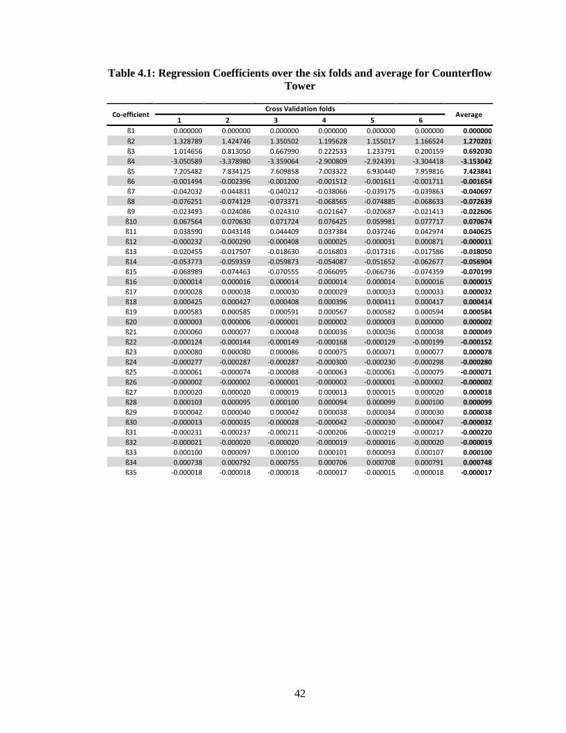
tower is shown in Figure 4.3. The 35 coefficients obtained for each regression over each
fold for a counter flow tower and a cross flow tower are as shown in Table 4.1 and Table
4.2 respectively. It is seen that the coefficients are fairly similar on each regression test.
This reinforces our belief that we are not overfitting the model. The results are then
averaged out over the six folds and used to verify the model.
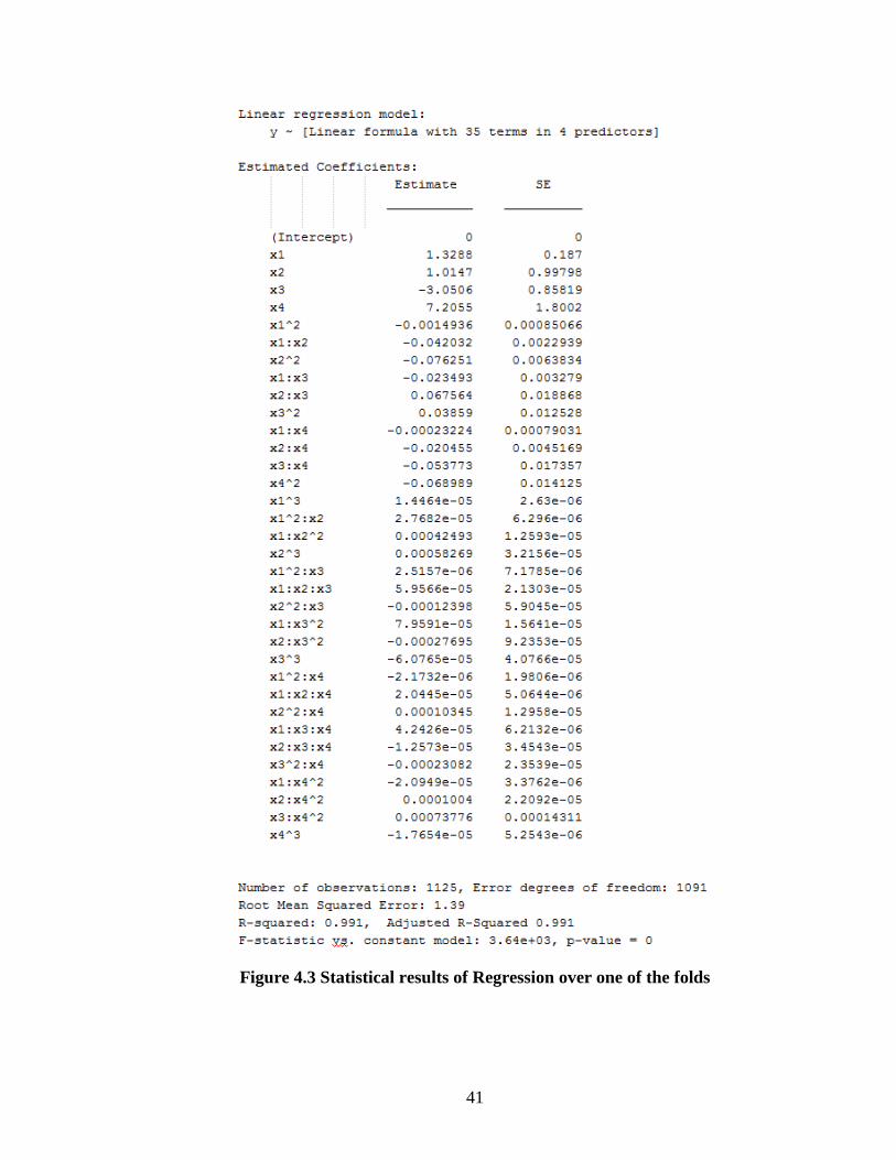
41
Figure 4.3 Statistical results of Regression over one of the folds
42
Table 4.1: Regression Coefficients over the six folds and average for Counterflow
Tower
1 2 3 4 5 6
ß1 0.000000 0.000000 0.000000 0.000000 0.000000 0.000000 0.000000
ß2 1.328789 1.424746 1.350502 1.195628 1.155017 1.166524 1.270201
ß3 1.014656 0.813050 0.667990 0.222533 1.233791 0.200159 0.692030
ß4 -3.050589 -3.378980 -3.359064 -2.900809 -2.924391 -3.304418 -3.153042
ß5 7.205482 7.834125 7.609858 7.003322 6.930440 7.959816 7.423841
ß6 -0.001494 -0.002396 -0.001200 -0.001512 -0.001611 -0.001711 -0.001654
ß7 -0.042032 -0.044831 -0.040212 -0.038066 -0.039175 -0.039863 -0.040697
ß8 -0.076251 -0.074129 -0.073371 -0.068565 -0.074885 -0.068633 -0.072639
ß9 -0.023493 -0.024086 -0.024310 -0.021647 -0.020687 -0.021413 -0.022606
ß10 0.067564 0.070630 0.071724 0.076425 0.059981 0.077717 0.070674
ß11 0.038590 0.043148 0.044409 0.037384 0.037246 0.042974 0.040625
ß12 -0.000232 -0.000290 -0.000408 0.000025 -0.000031 0.000871 -0.000011
ß13 -0.020455 -0.017507 -0.018630 -0.016803 -0.017316 -0.017586 -0.018050
ß14 -0.053773 -0.059359 -0.059873 -0.054087 -0.051652 -0.062677 -0.056904
ß15 -0.068989 -0.074463 -0.070555 -0.066095 -0.066736 -0.074359 -0.070199
ß16 0.000014 0.000016 0.000014 0.000014 0.000014 0.000016 0.000015
ß17 0.000028 0.000038 0.000030 0.000029 0.000033 0.000033 0.000032
ß18 0.000425 0.000427 0.000408 0.000396 0.000411 0.000417 0.000414
ß19 0.000583 0.000585 0.000591 0.000567 0.000582 0.000594 0.000584
ß20 0.000003 0.000006 -0.000001 0.000002 0.000003 0.000000 0.000002
ß21 0.000060 0.000077 0.000048 0.000036 0.000036 0.000038 0.000049
ß22 -0.000124 -0.000144 -0.000149 -0.000168 -0.000129 -0.000199 -0.000152
ß23 0.000080 0.000080 0.000086 0.000075 0.000071 0.000077 0.000078
ß24 -0.000277 -0.000287 -0.000287 -0.000300 -0.000230 -0.000298 -0.000280
ß25 -0.000061 -0.000074 -0.000088 -0.000063 -0.000061 -0.000079 -0.000071
ß26 -0.000002 -0.000002 -0.000001 -0.000002 -0.000001 -0.000002 -0.000002
ß27 0.000020 0.000020 0.000019 0.000013 0.000015 0.000020 0.000018
ß28 0.000103 0.000095 0.000100 0.000094 0.000099 0.000100 0.000099
ß29 0.000042 0.000040 0.000042 0.000038 0.000034 0.000030 0.000038
ß30 -0.000013 -0.000035 -0.000028 -0.000042 -0.000030 -0.000047 -0.000032
ß31 -0.000231 -0.000237 -0.000211 -0.000206 -0.000219 -0.000217 -0.000220
ß32 -0.000021 -0.000020 -0.000020 -0.000019 -0.000016 -0.000020 -0.000019
ß33 0.000100 0.000097 0.000100 0.000101 0.000093 0.000107 0.000100
ß34 0.000738 0.000792 0.000755 0.000706 0.000708 0.000791 0.000748
ß35 -0.000018 -0.000018 -0.000018 -0.000017 -0.000015 -0.000018 -0.000017
Cross Validation foldsCo-efficient Average
43
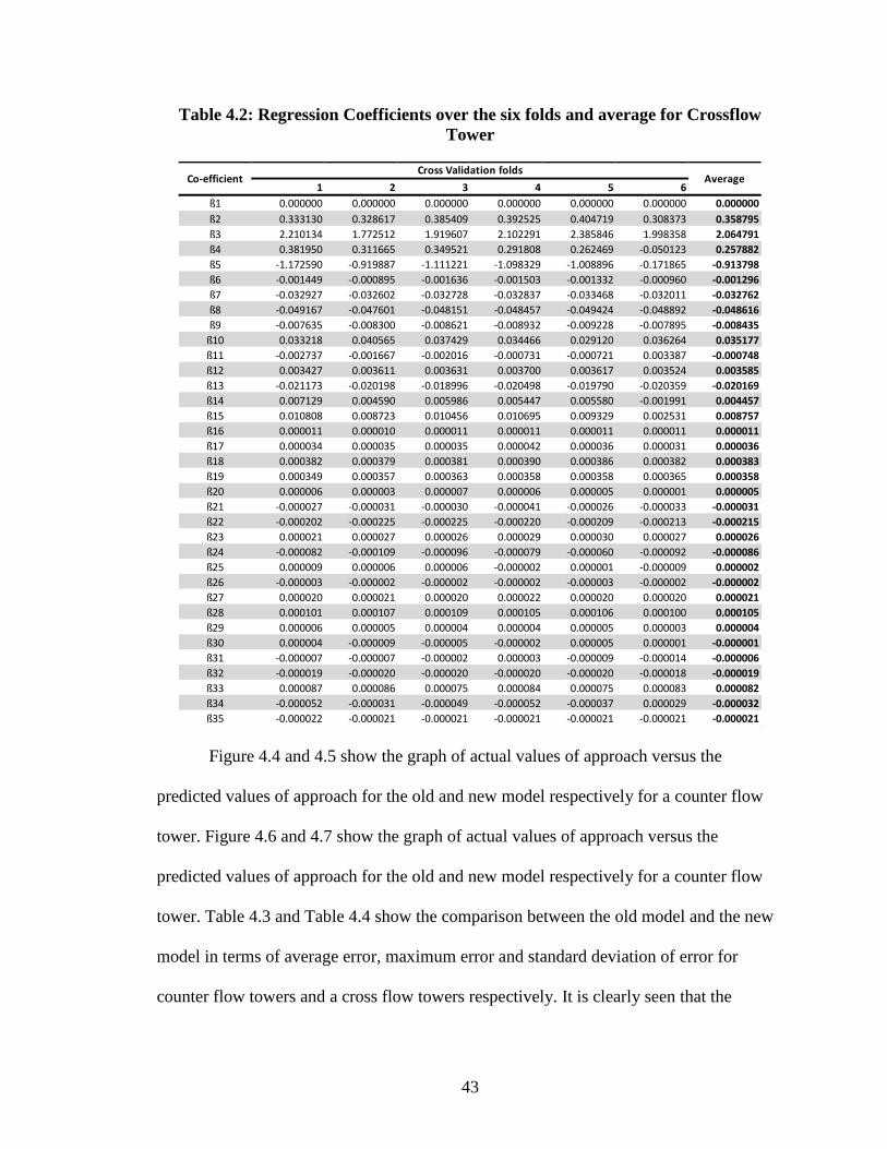
Table 4.2: Regression Coefficients over the six folds and average for Crossflow
Tower
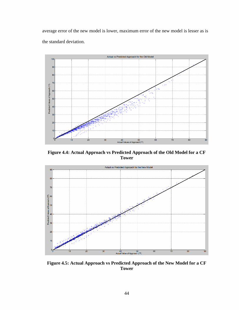
Figure 4.4 and 4.5 show the graph of actual values of approach versus the
predicted values of approach for the old and new model respectively for a counter flow
tower. Figure 4.6 and 4.7 show the graph of actual values of approach versus the
predicted values of approach for the old and new model respectively for a counter flow
tower. Table 4.3 and Table 4.4 show the comparison between the old model and the new
model in terms of average error, maximum error and standard deviation of error for
counter flow towers and a cross flow towers respectively. It is clearly seen that the
1 2 3 4 5 6
ß1 0.000000 0.000000 0.000000 0.000000 0.000000 0.000000 0.000000
ß2 0.333130 0.328617 0.385409 0.392525 0.404719 0.308373 0.358795
ß3 2.210134 1.772512 1.919607 2.102291 2.385846 1.998358 2.064791
ß4 0.381950 0.311665 0.349521 0.291808 0.262469 -0.050123 0.257882
ß5 -1.172590 -0.919887 -1.111221 -1.098329 -1.008896 -0.171865 -0.913798
ß6 -0.001449 -0.000895 -0.001636 -0.001503 -0.001332 -0.000960 -0.001296
ß7 -0.032927 -0.032602 -0.032728 -0.032837 -0.033468 -0.032011 -0.032762
ß8 -0.049167 -0.047601 -0.048151 -0.048457 -0.049424 -0.048892 -0.048616
ß9 -0.007635 -0.008300 -0.008621 -0.008932 -0.009228 -0.007895 -0.008435
ß10 0.033218 0.040565 0.037429 0.034466 0.029120 0.036264 0.035177
ß11 -0.002737 -0.001667 -0.002016 -0.000731 -0.000721 0.003387 -0.000748
ß12 0.003427 0.003611 0.003631 0.003700 0.003617 0.003524 0.003585
ß13 -0.021173 -0.020198 -0.018996 -0.020498 -0.019790 -0.020359 -0.020169
ß14 0.007129 0.004590 0.005986 0.005447 0.005580 -0.001991 0.004457
ß15 0.010808 0.008723 0.010456 0.010695 0.009329 0.002531 0.008757
ß16 0.000011 0.000010 0.000011 0.000011 0.000011 0.000011 0.000011
ß17 0.000034 0.000035 0.000035 0.000042 0.000036 0.000031 0.000036
ß18 0.000382 0.000379 0.000381 0.000390 0.000386 0.000382 0.000383
ß19 0.000349 0.000357 0.000363 0.000358 0.000358 0.000365 0.000358
ß20 0.000006 0.000003 0.000007 0.000006 0.000005 0.000001 0.000005
ß21 -0.000027 -0.000031 -0.000030 -0.000041 -0.000026 -0.000033 -0.000031
ß22 -0.000202 -0.000225 -0.000225 -0.000220 -0.000209 -0.000213 -0.000215
ß23 0.000021 0.000027 0.000026 0.000029 0.000030 0.000027 0.000026
ß24 -0.000082 -0.000109 -0.000096 -0.000079 -0.000060 -0.000092 -0.000086
ß25 0.000009 0.000006 0.000006 -0.000002 0.000001 -0.000009 0.000002
ß26 -0.000003 -0.000002 -0.000002 -0.000002 -0.000003 -0.000002 -0.000002
ß27 0.000020 0.000021 0.000020 0.000022 0.000020 0.000020 0.000021
ß28 0.000101 0.000107 0.000109 0.000105 0.000106 0.000100 0.000105
ß29 0.000006 0.000005 0.000004 0.000004 0.000005 0.000003 0.000004
ß30 0.000004 -0.000009 -0.000005 -0.000002 0.000005 0.000001 -0.000001
ß31 -0.000007 -0.000007 -0.000002 0.000003 -0.000009 -0.000014 -0.000006
ß32 -0.000019 -0.000020 -0.000020 -0.000020 -0.000020 -0.000018 -0.000019
ß33 0.000087 0.000086 0.000075 0.000084 0.000075 0.000083 0.000082
ß34 -0.000052 -0.000031 -0.000049 -0.000052 -0.000037 0.000029 -0.000032
ß35 -0.000022 -0.000021 -0.000021 -0.000021 -0.000021 -0.000021 -0.000021
Co-efficientCross Validation folds
Average
44
average error of the new model is lower, maximum error of the new model is lesser as is
the standard deviation.
Figure 4.4: Actual Approach vs Predicted Approach of the Old Model for a CF
Tower
Figure 4.5: Actual Approach vs Predicted Approach of the New Model for a CF
Tower

45
Figure 4.6: Actual Approach vs Predicted Approach of the Old Model for a XF
Tower
Figure 4.7: Actual Approach vs Predicted Approach of the New Model for a XF
Tower
46
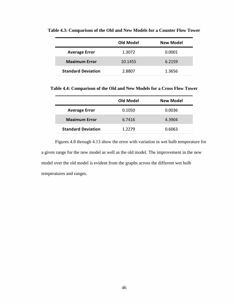
Table 4.3: Comparison of the Old and New Models for a Counter Flow Tower
Table 4.4: Comparison of the Old and New Models for a Cross Flow Tower
Figures 4.8 through 4.13 show the error with variation in wet bulb temperature for
a given range for the new model as well as the old model. The improvement in the new
model over the old model is evident from the graphs across the different wet bulb
temperatures and ranges.
Old Model New Model
Average Error 1.3072 0.0001
Maximum Error 10.1455 6.2159
Standard Deviation 2.8807 1.3656
Old Model New Model
Average Error 0.1050 0.0036
Maximum Error 6.7416 4.3904
Standard Deviation 1.2279 0.6063

47
Figure 4.8: Comparison of Error between the old and new model at Range=15°F for
a Counter Flow Tower
Figure 4.9: Comparison of Error between the old and new model at Range=15°F for
a Counter Flow Tower

48
Figure 4.10: Comparison of Error between the old and new model at Range=10°F
for a Counter Flow Tower
Figure 4.11: Comparison of Error between the old and new model at Range=10°F
for a Counter Flow Tower

49
Figure 4.12: Comparison of Error between the old and new model at Range=5°F for
a Counter Flow Tower
Figure 4.13: Comparison of Error between the old and new model at Range=5°F for
a Counter Flow Tower
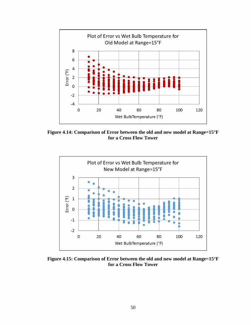
50
Figure 4.14: Comparison of Error between the old and new model at Range=15°F
for a Cross Flow Tower
Figure 4.15: Comparison of Error between the old and new model at Range=15°F
for a Cross Flow Tower
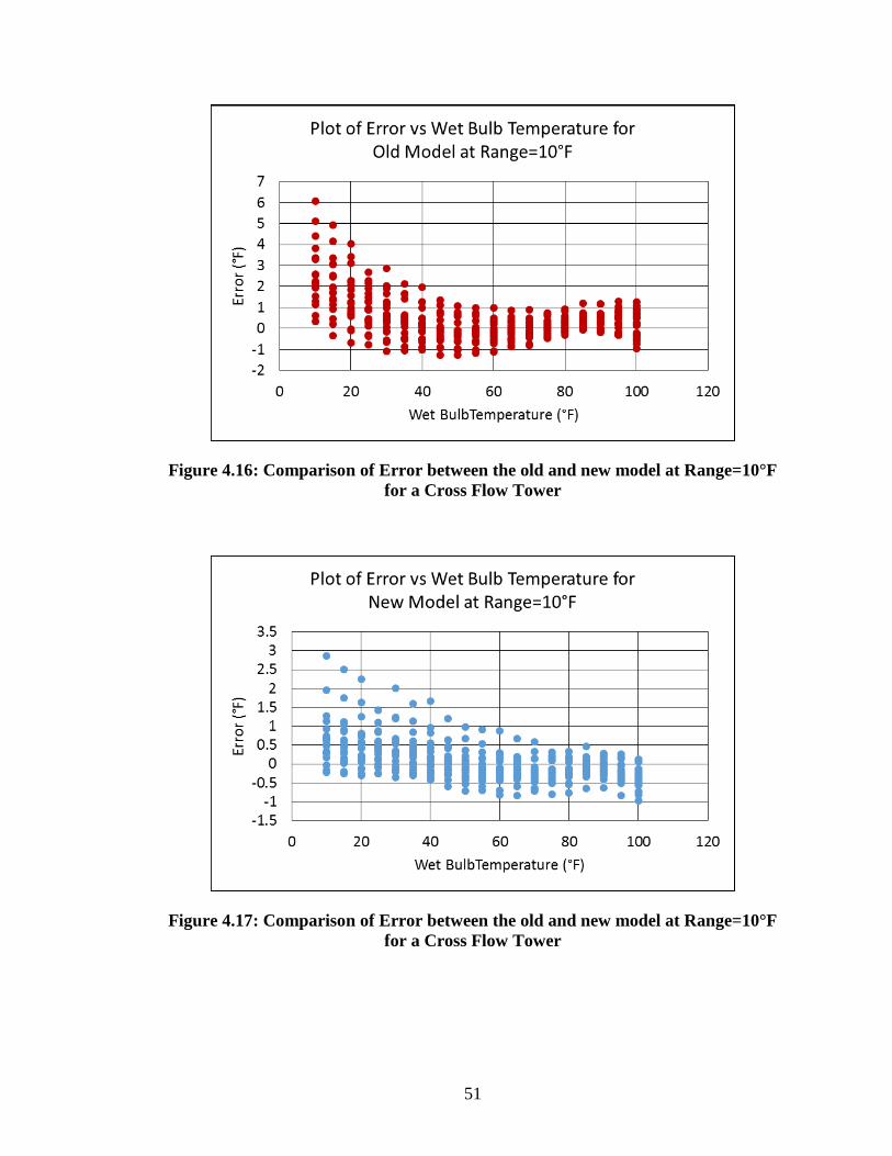
51
Figure 4.16: Comparison of Error between the old and new model at Range=10°F
for a Cross Flow Tower
Figure 4.17: Comparison of Error between the old and new model at Range=10°F
for a Cross Flow Tower
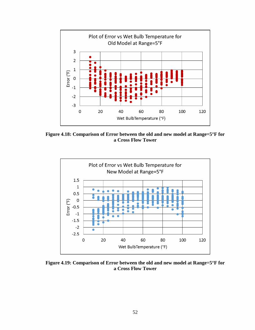
52
Figure 4.18: Comparison of Error between the old and new model at Range=5°F for
a Cross Flow Tower
Figure 4.19: Comparison of Error between the old and new model at Range=5°F for
a Cross Flow Tower

53
4.3 New Model Creation through Artificial Neural Networks
To check if ANNs are a feasible method to create a prediction model for cooling
towers, counter flow cooling tower data will be used to create a new model and the
results compared. The neural network toolbox in MATLAB was used for creating ANNs.
A neural network fitting tool was used. In a way similar to cross validation, the data is
split into 3 subsets of training data (70%), validation data (15%) and testing data (15%).
The ANN was trained with the training data during which the network weights and
functions are adjusted. Next the ANN is validated with the validation data to measure
network generalization and to halt training when generalization stops improving. The
testing data has no effect on training and is used to provide an independent measure of
network performance during and after training. The ANN is created with one hidden
layer of neurons. If there is no hidden layer of neurons, only linear separable functions
can be represented using that ANN. Having one layer of hidden neurons can approximate
most continuous functions. Adding additional hidden layers may increase accuracy in
some cases, but will require greater computational effort and may also lead to over
fitting. The ANN was trained using the Levenberg-Marquardt backpropagation
algorithm. The results obtained for a neural network model for counter flow tower with
one hidden layer are shown below. Figure 4.20 shows the error histogram, Figure 4.21
shows the performance of the neural network and Figure 4.22 gives the regression plots.

54
Figure 4.20: Error Histogram for Neural Network Fitting with One Hidden layer of
Neurons
Figure 4.21: Performance for Neural Network Fitting with One Hidden layer of
Neurons

55
Figure 4.22: Regression Plots for Neural Network Fitting with One Hidden layer of
Neurons
The ANN is created again, but now with two layers. The results obtained are as follows

56
Figure 4.23: Error Histogram for Neural Network Fitting with Two Hidden layers
of Neurons
Figure 4.24: Performance for Neural Network Fitting with Two Hidden layers of
Neurons

57
Figure 4.25: Regression Plots for Neural Network Fitting with Two Hidden layers of
Neurons
It is seen that the prediction error was decreased by increasing the hidden layer of
neurons to two and a better prediction is achieved. According to MATLAB, an epoch is a
measure of the number of times all of the training vectors are used once to update the
weights. For batch training all of the training samples pass through the learning algorithm
simultaneously in one epoch before weights are updated. Thus by increasing the number
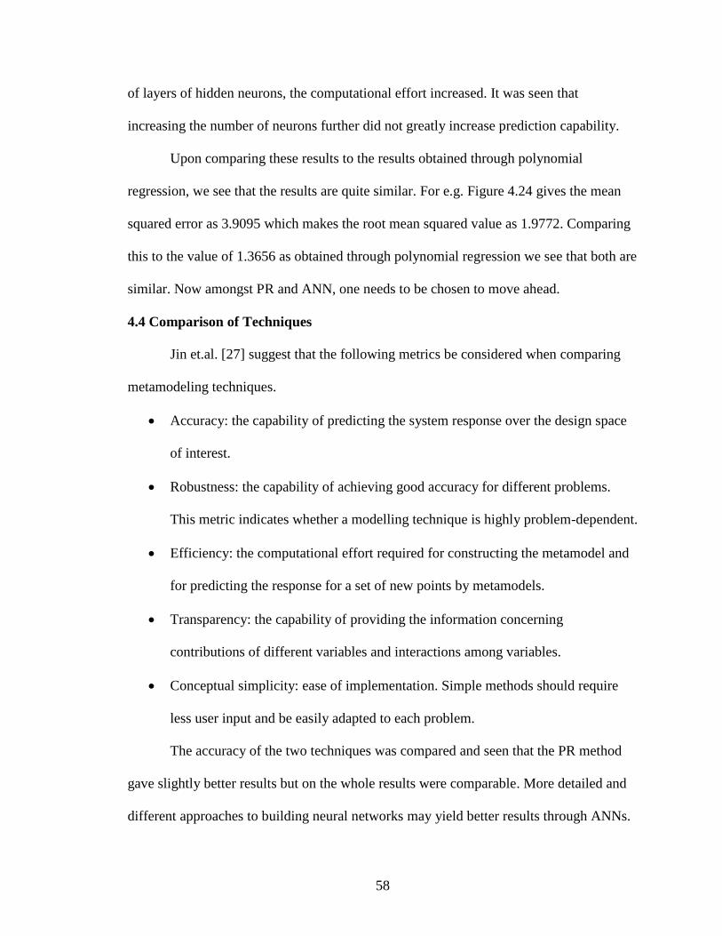
58
of layers of hidden neurons, the computational effort increased. It was seen that
increasing the number of neurons further did not greatly increase prediction capability.
Upon comparing these results to the results obtained through polynomial
regression, we see that the results are quite similar. For e.g. Figure 4.24 gives the mean
squared error as 3.9095 which makes the root mean squared value as 1.9772. Comparing
this to the value of 1.3656 as obtained through polynomial regression we see that both are
similar. Now amongst PR and ANN, one needs to be chosen to move ahead.
4.4 Comparison of Techniques
Jin et.al. [27] suggest that the following metrics be considered when comparing
metamodeling techniques.
Accuracy: the capability of predicting the system response over the design space
of interest.
Robustness: the capability of achieving good accuracy for different problems.
This metric indicates whether a modelling technique is highly problem-dependent.
Efficiency: the computational effort required for constructing the metamodel and
for predicting the response for a set of new points by metamodels.
Transparency: the capability of providing the information concerning
contributions of different variables and interactions among variables.
Conceptual simplicity: ease of implementation. Simple methods should require
less user input and be easily adapted to each problem.
The accuracy of the two techniques was compared and seen that the PR method
gave slightly better results but on the whole results were comparable. More detailed and
different approaches to building neural networks may yield better results through ANNs.

59
As seen in the literature review earlier PR technique has been used before
(Benton et.al and DOE2 engine) to create surrogate models for this particular situation to
good effect and is thus a good choice for moving forward. It is seen that ANN is also a
suitable method to create a prediction model for cooling tower performance based on
results obtained.
PR is a more widely used technique compared to ANN and also requires lesser
computational effort [21]. Further PR is much simpler and quicker to implement than
ANN.
The CWSAT currently uses a model created through third order polynomial
regression. Utilizing a similar new model will allow for a much simpler improvement of
CWSAT as well. While the ANN technique allows another method of creating a model
and has the advantage of being able to train the neural network with newer data as
available, implementing a neural network model outside (e.g. in CWSAT) of software
built specifically for neural networks would require additional effort. Thus the PR
technique will be employed to create a new model at this stage for the sake of simplicity
and possibility of easier implementation in CWSAT.
60
CHAPTER 5
WATER SIDE ECONOMIZER / FREE COOLING
This chapter explains the reduction in capacity of cooling towers when operated
in free cooling mode. The new and old models are used to simulate tower performance
over a year and differences are noted. Also the economic benefits of having larger
cooling tower capacity to accomplish free cooling are analyzed.
5.1 Reduction in Cooling Tower Capacity at Low Temperatures
It seems counter intuitive that the cooling tower capacity drops when the tower is
operated in free cooling mode at low temperatures. The reason this occurs goes back to
the point addressed in the introduction that the cooling tower works primarily on the
principle of evaporative cooling. As the temperature drops, the amount of water that the
air can hold also drops significantly. Since the tower can no longer reject as much heat to
atmosphere through the evaporation of water, the tower capacity drops. It is also to be
noted that there is some heat transfer to atmosphere through sensible heat transfer as a
result of the temperature difference. During free cooling conditions the sensible heat
transfer is not large because the water entering the cooling tower is quite close to the
atmospheric dry bulb temperature. This is the reason for reduced cooling tower capacity
when operating the tower in free cooling mode.
This can also be illustrated with some numbers. Consider the standard conditions
that a tower is rated at; 95°F entering water temperature (EWT), 85°F leaving water
temperature (LWT) and a wet bulb temperature of 78°F. For the location of Boston,
TMY2 (Typical Meteorological Year) data was obtained and the average relative
humidity (RH) for the summer months from May to October was found to be 68.5%. At a

61
wet bulb temperature of 78°F and a RH of 68.5% we find the humidity ratio to be
0.01875 lb/lb (the units are pounds moisture per pound dry air). Assuming that
evaporative cooling is taking place and the air leaves the cooling tower in a saturated
condition i.e. 100%RH (one of the assumptions of Merkel theory) we have the humidity
ratio of air leaving the tower as 0.02078 lb/lb. The amount of moisture increase is
2.03*10-3.
It is seen that the winter months from November to April have an average RH of
63%. In most cases the chilled water set point temperature (CHWST) for the chiller is
45°F. If we have to substitute the chiller with the tower, the tower should be able to
produce water at 45°F. For the ideal case we can assume that the water reaches the wet
bulb temperature and we also need to account for the temperature drop across a heat
exchanger that may be used.
wbFCT CHWST HEX
If we assume a temperature drop of 4°F across the heat exchanger, then the wet
bulb temperature that is required for us to be able to perform free cooling is 41°F. At a
wet bulb temperature of 41°F and a RH of 63% we find the humidity ratio to be 0.00418
lb/lb. Assuming that evaporative cooling is taking place and the air leaves the cooling
tower in a saturated condition we have the humidity ratio of air leaving the tower as
0.0054 lb/lb. The amount of moisture increase is 1.22*10-3. This is almost half of that in
the earlier case. Table 5.1 shows the conditions of air entering and leaving the tower for
both summer and winter to present the number in a clear and concise manner. Figure 5.1
shows the conditions of air entering and leaving the tower in summer and winter on a
psychrometric chart to better illustrate the decreased amount of water vapor the air can
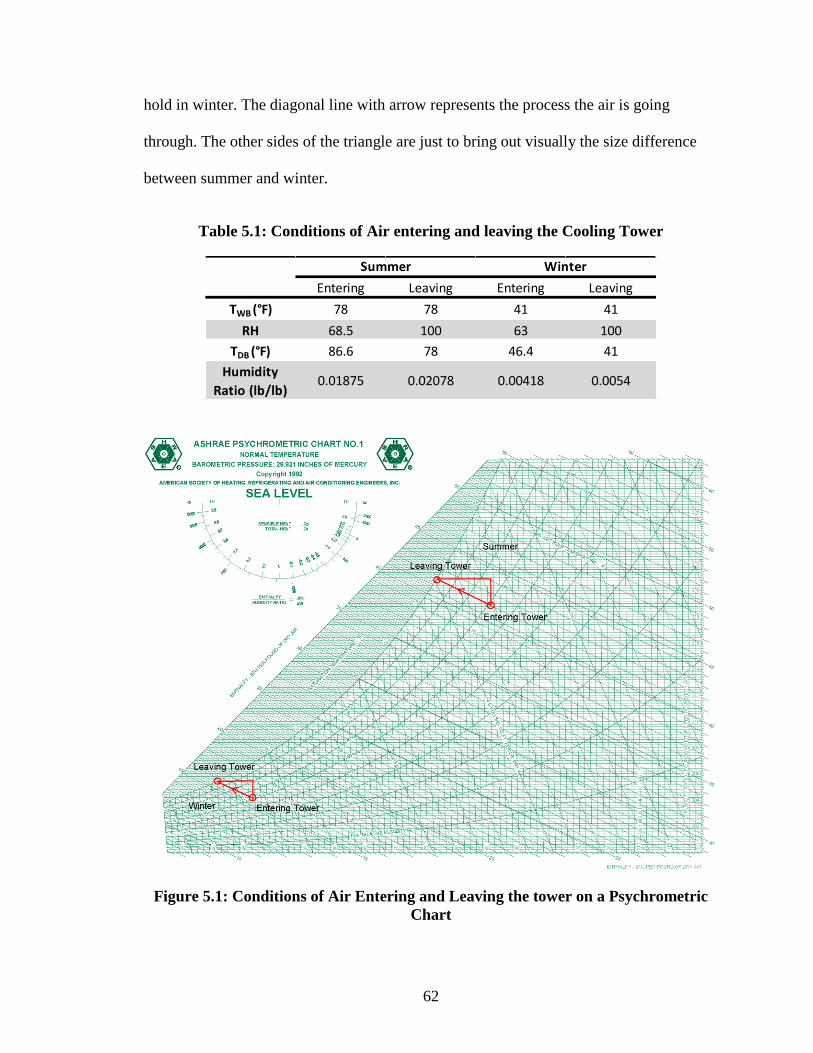
62
hold in winter. The diagonal line with arrow represents the process the air is going
through. The other sides of the triangle are just to bring out visually the size difference
between summer and winter.
Table 5.1: Conditions of Air entering and leaving the Cooling Tower
Figure 5.1: Conditions of Air Entering and Leaving the tower on a Psychrometric
Chart
Entering Leaving Entering Leaving
TWB (°F) 78 78 41 41
RH 68.5 100 63 100
TDB (°F) 86.6 78 46.4 41
Humidity
Ratio (lb/lb)0.01875 0.02078 0.00418 0.0054
Summer Winter
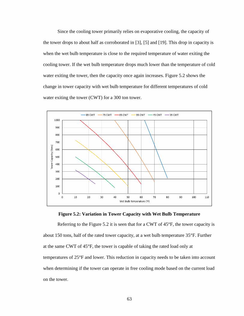
63
Since the cooling tower primarily relies on evaporative cooling, the capacity of
the tower drops to about half as corroborated in [3], [5] and [19]. This drop in capacity is
when the wet bulb temperature is close to the required temperature of water exiting the
cooling tower. If the wet bulb temperature drops much lower than the temperature of cold
water exiting the tower, then the capacity once again increases. Figure 5.2 shows the
change in tower capacity with wet bulb temperature for different temperatures of cold
water exiting the tower (CWT) for a 300 ton tower.
Figure 5.2: Variation in Tower Capacity with Wet Bulb Temperature
Referring to the Figure 5.2 it is seen that for a CWT of 45°F, the tower capacity is
about 150 tons, half of the rated tower capacity, at a wet bulb temperature 35°F. Further
at the same CWT of 45°F, the tower is capable of taking the rated load only at
temperatures of 25°F and lower. This reduction in capacity needs to be taken into account
when determining if the tower can operate in free cooling mode based on the current load
on the tower.

64
5.2 Comparison of Prediction Capability of the different Models
To compare the old and new models, code is written in MATLAB and given in
Appendix B. This code simulates the tower performance round the year. The same code
is utilized to simulate tower performance for both the old and new models. A comparison
is made with the results obtained from CWSAT to ascertain if the model is appropriately
implemented (Note: The old model and the CWSAT utilize the same regression model
for a crossflow tower. The reason for choosing to compare the old model outside of
CWSAT is to determine if CWSAT is working appropriately). The tower is assumed to
be a cross flow tower since that is the regression model that is used in the CWSAT
program.
The chiller is assumed to be loaded according to the Air-Conditioning &
Refrigeration Institute (ARI) schedule which imposes a corresponding load on the tower.
Table 5.2 shows the number of hours the chiller is at a particular load annually according
to the ARI schedule. The input parameters are given in Table 5.3. CWSAT is also used to
simulate tower performance for the same conditions. A 300 ton tower is needed for a 250
ton chiller because the tower needs to reject an additional amount of heat apart from the
load on the chiller which is the heat of compression of the chiller. For the current case, a
heat of compression of 20% of the current load is utilized which yields a tower size
requirement of 300 tons. From looking at specifications of 300 ton cooling towers, it is
determined that they have a fan of 25 hp.
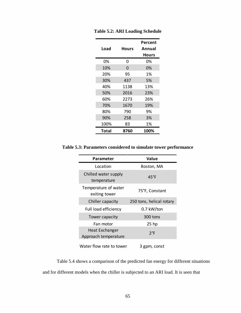
65
Table 5.2: ARI Loading Schedule
Table 5.3: Parameters considered to simulate tower performance
Table 5.4 shows a comparison of the predicted fan energy for different situations
and for different models when the chiller is subjected to an ARI load. It is seen that
Load Hours
Percent
Annual
Hours
0% 0 0%
10% 0 0%
20% 95 1%
30% 437 5%
40% 1138 13%
50% 2016 23%
60% 2273 26%
70% 1670 19%
80% 790 9%
90% 258 3%
100% 83 1%
Total 8760 100%
Parameter Value
Location Boston, MA
Chilled water supply
temperature45°F
Temperature of water
exiting tower75°F, Constant
Chiller capacity 250 tons, helical rotary
Full load efficiency 0.7 kW/ton
Tower capacity 300 tons
Fan motor 25 hp
Heat Exchanger
Approach temperature2°F
Water flow rate to tower 3 gpm, const
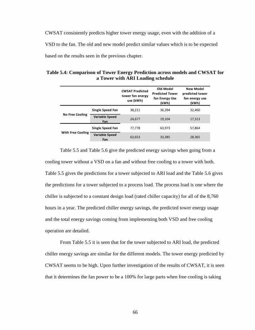
66
CWSAT consistently predicts higher tower energy usage, even with the addition of a
VSD to the fan. The old and new model predict similar values which is to be expected
based on the results seen in the previous chapter.
Table 5.4: Comparison of Tower Energy Prediction across models and CWSAT for
a Tower with ARI Loading schedule
Table 5.5 and Table 5.6 give the predicted energy savings when going from a
cooling tower without a VSD on a fan and without free cooling to a tower with both.
Table 5.5 gives the predictions for a tower subjected to ARI load and the Table 5.6 gives
the predictions for a tower subjected to a process load. The process load is one where the
chiller is subjected to a constant design load (rated chiller capacity) for all of the 8,760
hours in a year. The predicted chiller energy savings, the predicted tower energy usage
and the total energy savings coming from implementing both VSD and free cooling
operation are detailed.
From Table 5.5 it is seen that for the tower subjected to ARI load, the predicted
chiller energy savings are similar for the different models. The tower energy predicted by
CWSAT seems to be high. Upon further investigation of the results of CWSAT, it is seen
that it determines the fan power to be a 100% for large parts when free cooling is taking
CWSAT Predicted
tower fan energy
use (kWh)
Old Model
Predicted Tower
fan Energy Use
(kWh)
New Model
predicted tower
fan energy use
(kWh)
Single Speed Fan 38,211 36,394 32,460
Variable Speed
Fan24,677 19,104 17,313
Single Speed Fan 77,778 63,973 57,864
Variable Speed
Fan63,653 33,385 28,365
No Free Cooling
With Free Cooling
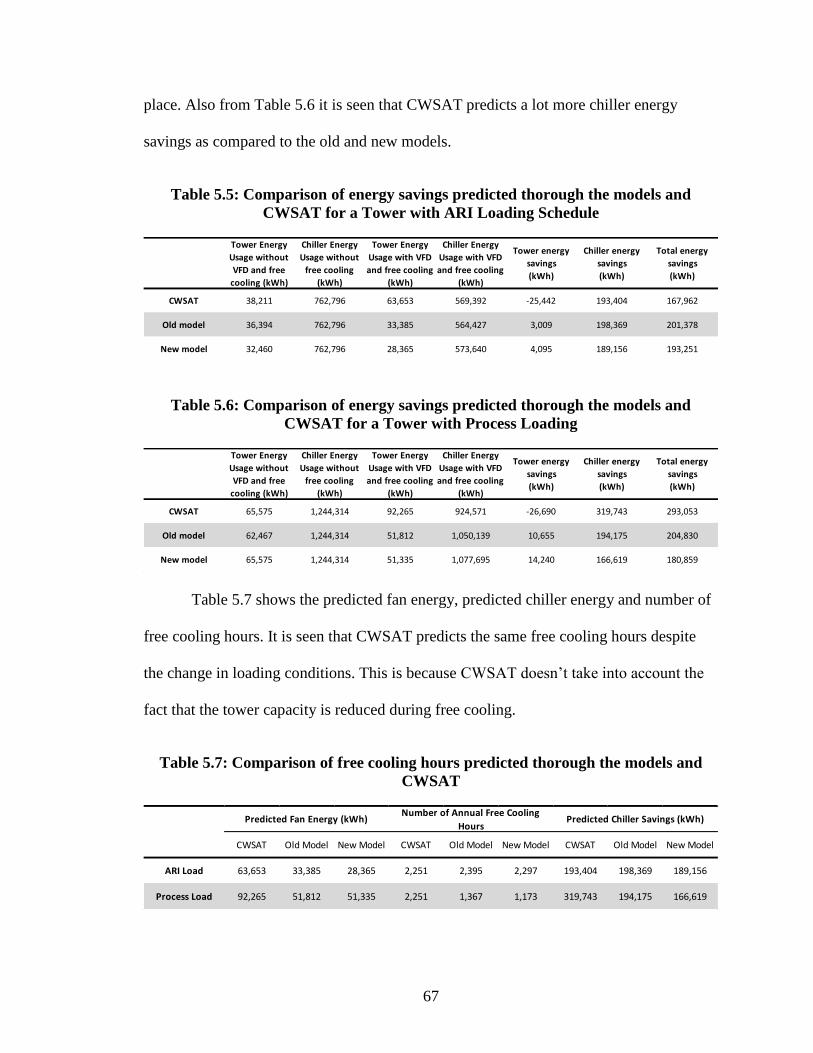
67
place. Also from Table 5.6 it is seen that CWSAT predicts a lot more chiller energy
savings as compared to the old and new models.
Table 5.5: Comparison of energy savings predicted thorough the models and
CWSAT for a Tower with ARI Loading Schedule
Table 5.6: Comparison of energy savings predicted thorough the models and
CWSAT for a Tower with Process Loading
Table 5.7 shows the predicted fan energy, predicted chiller energy and number of
free cooling hours. It is seen that CWSAT predicts the same free cooling hours despite
the change in loading conditions. This is because CWSAT doesn’t take into account the
fact that the tower capacity is reduced during free cooling.
Table 5.7: Comparison of free cooling hours predicted thorough the models and
CWSAT
Tower Energy
Usage without
VFD and free
cooling (kWh)
Chiller Energy
Usage without
free cooling
(kWh)
Tower Energy
Usage with VFD
and free cooling
(kWh)
Chiller Energy
Usage with VFD
and free cooling
(kWh)
Tower energy
savings
(kWh)
Chiller energy
savings
(kWh)
Total energy
savings
(kWh)
CWSAT 38,211 762,796 63,653 569,392 -25,442 193,404 167,962
Old model 36,394 762,796 33,385 564,427 3,009 198,369 201,378
New model 32,460 762,796 28,365 573,640 4,095 189,156 193,251
Tower Energy
Usage without
VFD and free
cooling (kWh)
Chiller Energy
Usage without
free cooling
(kWh)
Tower Energy
Usage with VFD
and free cooling
(kWh)
Chiller Energy
Usage with VFD
and free cooling
(kWh)
Tower energy
savings
(kWh)
Chiller energy
savings
(kWh)
Total energy
savings
(kWh)
CWSAT 65,575 1,244,314 92,265 924,571 -26,690 319,743 293,053
Old model 62,467 1,244,314 51,812 1,050,139 10,655 194,175 204,830
New model 65,575 1,244,314 51,335 1,077,695 14,240 166,619 180,859
CWSAT Old Model New Model CWSAT Old Model New Model CWSAT Old Model New Model
ARI Load 63,653 33,385 28,365 2,251 2,395 2,297 193,404 198,369 189,156
Process Load 92,265 51,812 51,335 2,251 1,367 1,173 319,743 194,175 166,619
Predicted Fan Energy (kWh)Number of Annual Free Cooling
HoursPredicted Chiller Savings (kWh)

68
It is seen that considerable energy savings are possible through the use of a VSD
and operating the tower in economizer mode. Assuming a marginal cost of electricity at
$0.08/kWh, the results from the previous tables can be converted to cost savings as
shown in Table 5.8.
Table 5.8: Predicted Cost Savings associated with VSD and Free Cooling
Figures 5.3 to 5.5 show the variation in wet bulb temperature, percent fan power,
free cooling condition and the load on the chiller as predicted by CWSAT, old model and
new model respectively for a few hours in winter. Referring to Figure 5.3 for CWSAT
prediction, we see that the check for free cooling is completely based on temperature. If
the temperature is below a certain determined number, (that is constant based on the
required cooling water temperature and the drop across the heat exchanger) only then is
the tower assumed to be able to perform free cooling. Further, it is seen that as the load
on the chiller changes and the wet bulb temperature changes, there is almost no change in
the predicted fan power which is close to maximum (a value of greater than 100% for fan
power is seen because the VFD on the fan adds some losses). It can be seen between the
hours 27 and 39 that the load is continuously increasing while the wet bulb temperature is
fairly constant. CWSAT predicts maximum fan power usage at hour 27. If this is true,
increasing the load would mean that the tower would not be able to provide the required
cooling even at 100% fan power but CWSAT assumes that this is the case anyway which
CWSAT Old Model New Model
ARI Load $13,437 $16,110 $15,460
Process Load $23,444 $16,386 $14,469
Predicted Total Cost Savings
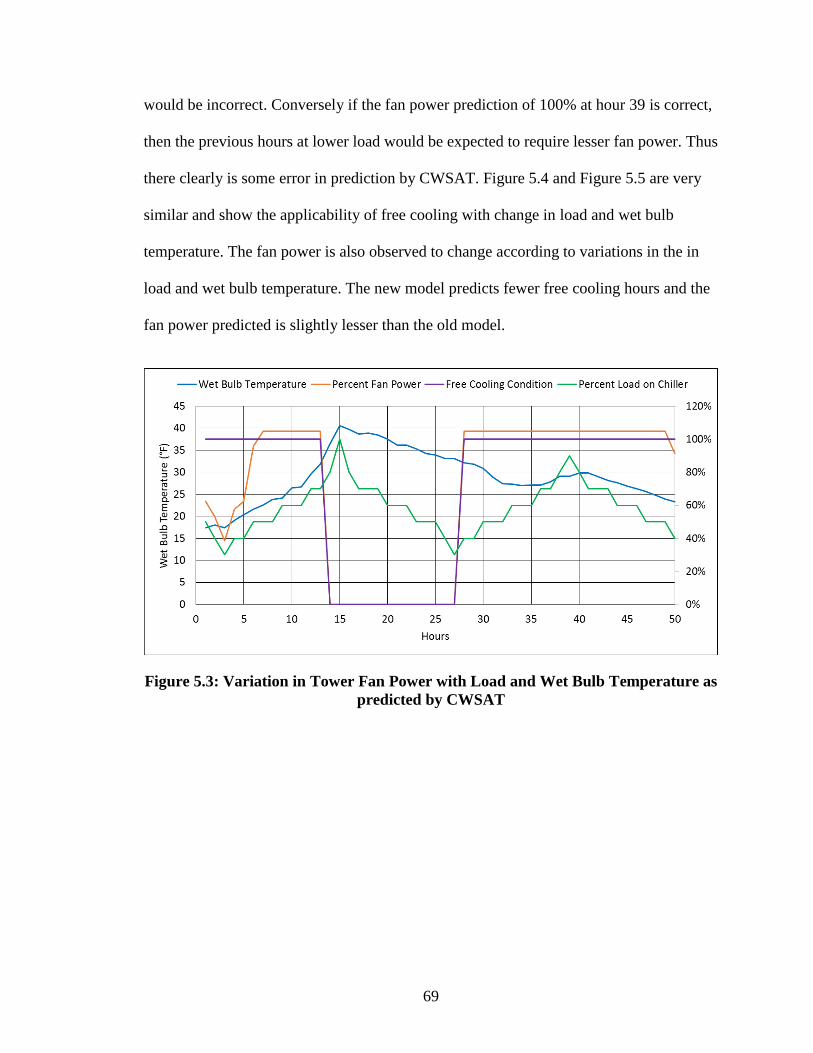
69
would be incorrect. Conversely if the fan power prediction of 100% at hour 39 is correct,
then the previous hours at lower load would be expected to require lesser fan power. Thus
there clearly is some error in prediction by CWSAT. Figure 5.4 and Figure 5.5 are very
similar and show the applicability of free cooling with change in load and wet bulb
temperature. The fan power is also observed to change according to variations in the in
load and wet bulb temperature. The new model predicts fewer free cooling hours and the
fan power predicted is slightly lesser than the old model.
Figure 5.3: Variation in Tower Fan Power with Load and Wet Bulb Temperature as
predicted by CWSAT

70
Figure 5.4: Variation in Tower Fan Power with Load and Wet Bulb Temperature as
predicted by the Old Model
Figure 5.5: Variation in Tower Fan Power with Load and Wet Bulb Temperature as
predicted by the New Model
5.3 Benefits of Larger Cooling Tower Capacity to meet Winter Load
We see from the Table 5.2 earlier that the annual the load on the tower is 50% or
lesser for 42% of the year. If we want to be able to carry out free cooling in winter when
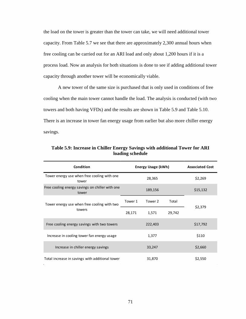
71
the load on the tower is greater than the tower can take, we will need additional tower
capacity. From Table 5.7 we see that there are approximately 2,300 annual hours when
free cooling can be carried out for an ARI load and only about 1,200 hours if it is a
process load. Now an analysis for both situations is done to see if adding additional tower
capacity through another tower will be economically viable.
A new tower of the same size is purchased that is only used in conditions of free
cooling when the main tower cannot handle the load. The analysis is conducted (with two
towers and both having VFDs) and the results are shown in Table 5.9 and Table 5.10.
There is an increase in tower fan energy usage from earlier but also more chiller energy
savings.
Table 5.9: Increase in Chiller Energy Savings with additional Tower for ARI
loading schedule
Condition Associated Cost
Tower energy use when free cooling with one
tower$2,269
Free cooling energy savings on chiller with one
tower$15,132
Tower 1 Tower 2 Total
28,171 1,571 29,742
Free cooling energy savings with two towers $17,792
Increase in cooling tower fan energy usage $110
Increase in chiller energy savings $2,660
Total increase in savings with additional tower $2,550
1,377
33,247
31,870
$2,379Tower energy use when free cooling with two
towers
Energy Usage (kWh)
28,365
189,156
222,403
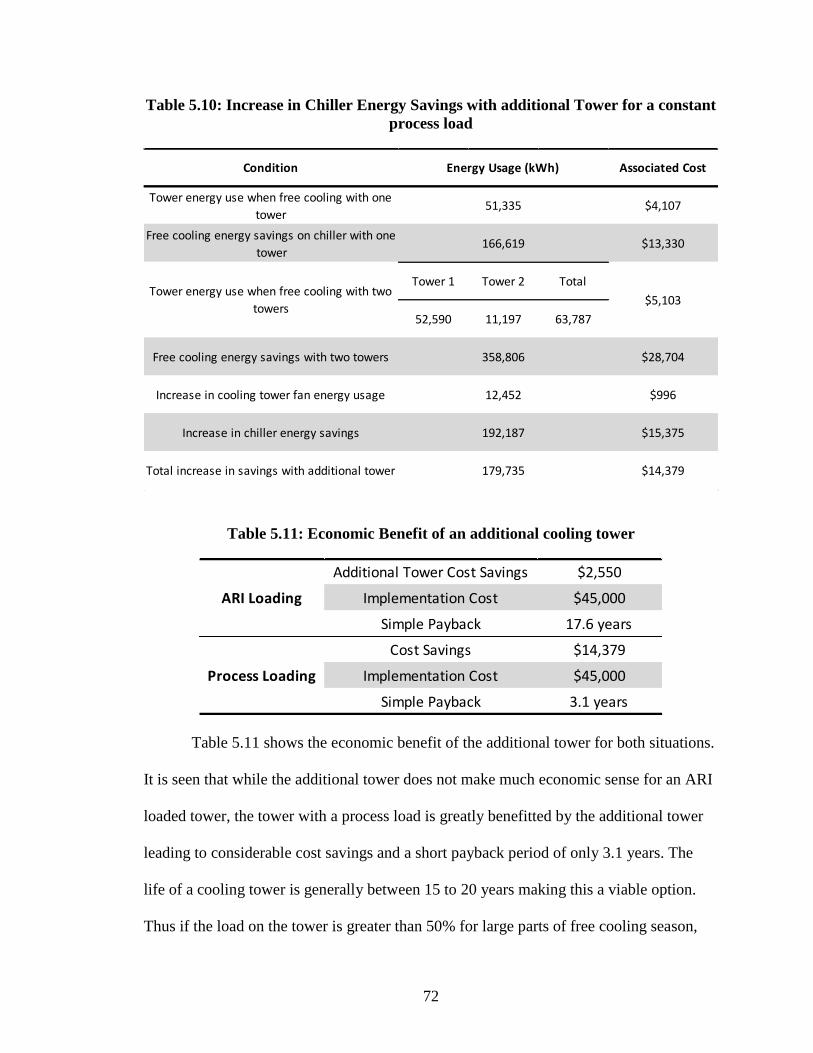
72
Table 5.10: Increase in Chiller Energy Savings with additional Tower for a constant
process load
Table 5.11: Economic Benefit of an additional cooling tower
Table 5.11 shows the economic benefit of the additional tower for both situations.
It is seen that while the additional tower does not make much economic sense for an ARI
loaded tower, the tower with a process load is greatly benefitted by the additional tower
leading to considerable cost savings and a short payback period of only 3.1 years. The
life of a cooling tower is generally between 15 to 20 years making this a viable option.
Thus if the load on the tower is greater than 50% for large parts of free cooling season,
Condition Associated Cost
Tower energy use when free cooling with one
tower$4,107
Free cooling energy savings on chiller with one
tower$13,330
Tower 1 Tower 2 Total
52,590 11,197 63,787
Free cooling energy savings with two towers $28,704
Increase in cooling tower fan energy usage $996
Increase in chiller energy savings $15,375
Total increase in savings with additional tower $14,379
$5,103
Energy Usage (kWh)
51,335
166,619
Tower energy use when free cooling with two
towers
358,806
12,452
192,187
179,735
Additional Tower Cost Savings $2,550
Implementation Cost $45,000
Simple Payback 17.6 years
Cost Savings $14,379
Implementation Cost $45,000
Simple Payback 3.1 years
Process Loading
ARI Loading
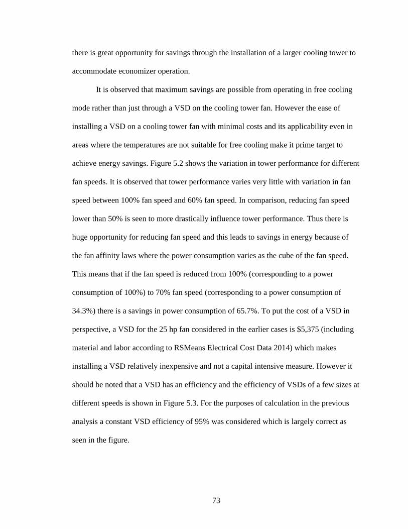
73
there is great opportunity for savings through the installation of a larger cooling tower to
accommodate economizer operation.
It is observed that maximum savings are possible from operating in free cooling
mode rather than just through a VSD on the cooling tower fan. However the ease of
installing a VSD on a cooling tower fan with minimal costs and its applicability even in
areas where the temperatures are not suitable for free cooling make it prime target to
achieve energy savings. Figure 5.2 shows the variation in tower performance for different
fan speeds. It is observed that tower performance varies very little with variation in fan
speed between 100% fan speed and 60% fan speed. In comparison, reducing fan speed
lower than 50% is seen to more drastically influence tower performance. Thus there is
huge opportunity for reducing fan speed and this leads to savings in energy because of
the fan affinity laws where the power consumption varies as the cube of the fan speed.
This means that if the fan speed is reduced from 100% (corresponding to a power
consumption of 100%) to 70% fan speed (corresponding to a power consumption of
34.3%) there is a savings in power consumption of 65.7%. To put the cost of a VSD in
perspective, a VSD for the 25 hp fan considered in the earlier cases is $5,375 (including
material and labor according to RSMeans Electrical Cost Data 2014) which makes
installing a VSD relatively inexpensive and not a capital intensive measure. However it
should be noted that a VSD has an efficiency and the efficiency of VSDs of a few sizes at
different speeds is shown in Figure 5.3. For the purposes of calculation in the previous
analysis a constant VSD efficiency of 95% was considered which is largely correct as
seen in the figure.
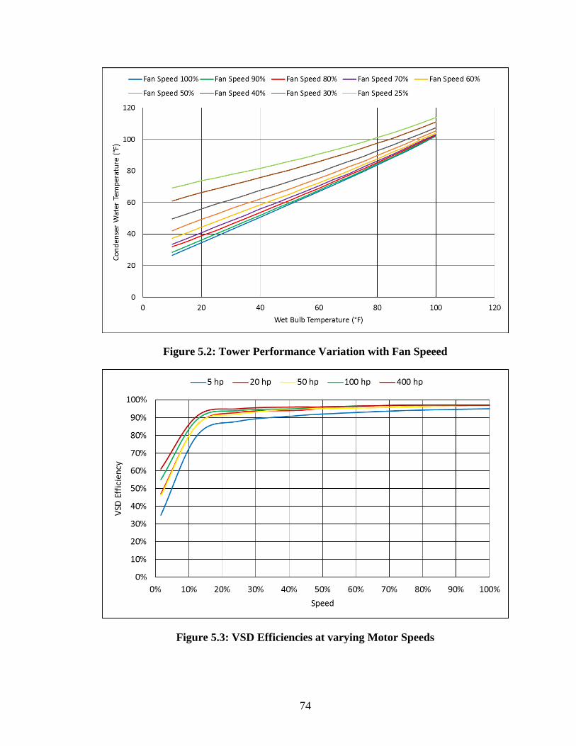
74
Figure 5.2: Tower Performance Variation with Fan Speeed
Figure 5.3: VSD Efficiencies at varying Motor Speeds

75
CHAPTER 6
CONCLUSIONS
This chapter includes recommendations for future work to the tool
5.1 Summary
In Chapter 2, the drawbacks of thermodynamic models and the need for simple
surrogate models was outlined. A simple to use model that requires easily available
information to predict tower fan energy use would be of great use to an average user.
Chapter 3 talked about the method and sources of data collection to verify the existing
model given by [2] and create a new model. Despite the difficulty of tower performance
data availability over a wide range of parameters, suitable information was collected to be
able to verify the existing model and create a new model.
Chapter 4 mapped out the method to create a new model and the results were
shown to be better than the previous model. Polynomial regression was found to be the
simplest yet accurate method to create a new model. The improvements though marginal
are found to be at those conditions where energy savings measures are possible leading to
a better prediction of savings.
In Chapter 5, CWSAT, the old model and the new model were used to predict
tower fan energy use over a year and the results were compared. Further the economic
benefit of adding an additional cooling tower was analyzed and found that greater the
load on the tower during times when the wet bulb temperature is lower than the required
cold water temperature, an additional tower clearly adds economic benefit.
76
5.2 Recommendations for Future Work
To check if CWSAT was implementing the old model correctly, separate code
was written to compare the results. It was seen that when the tower was not used in
economizer mode, the results obtained were close between the old model and CWSAT
(although CWSAT tended to predicted a higher value of fan power). When the tower is
operated in free cooling mode, it is seen that CWSAT does not take into account the load
on the tower but just the temperature. Making sure that CWSAT correctly accounts for
the load the tower can take will go a long way towards making more accurate predictions
of chiller energy savings. Further when hour by hour predicted fan power values were
analyzed, it was seen that during free cooling operation CWSAT always tended to predict
that the fan power required was almost always a 100% (much higher than needed).
Making sure that CWSAT correctly implements the model is of utmost importance in
being able to predict tower performance and thereby possible savings accurately.
As seen in Figure 5.2, the cooling tower performance is reduced considerably
when the fan speed is reduced below 60% (corresponds to 21.6% fan power). During
model building, data only until 60% fan speed was utilized since including lower fan
speeds tended to make predictions at higher speeds inaccurate. Thus when the model
predicts a low fan power (meaning low fan speeds), it might not always be possible in
reality to reduce the fan speed that low or turn off the fan completely. While this doesn’t
make much difference if the tower fan has a VSD, the fan power may add up over time
for a single speed fan. Going ahead it would be important to be able to determine what is
the lowest possible fan speed required without degrading tower performance, through

77
actual data collected from the field. Since ANNs were seen to give comparable accuracy
to PR, greater depth in looking at ANNs to create a prediction model might be beneficial.
The current version of CWSAT doesn’t allow choosing the kind of tower (i.e
counter flow or cross flow) and adding an option for that may be useful to be able to
predict tower performance more accurately. Finally adding an option in CWSAT to
predict additional savings possible through the use of an additional tower, especially for
process loads would make it an invaluable and complete tool to predict energy savings
associated with cooling towers.
Although CWSAT doesn’t need to be improved solely because of a new model
(the old and new model tend to give similar results), it needs to be spruced up to better
implement the existing model to more accurately predicted tower fan energy use. The
recommendations for future work may be summarized as follows
1. Check that CWSAT implements the tower performance prediction correctly and
makes sure that free cooling is possible by checking the maximum load that the
tower can take.
2. Determine how low the fan speed can actually be turned down since tower
performance degrades greatly at fan speeds lower than 50%.
3. Add an option in CWSAT to check if adding an additional tower is economically
viable.
4. Creating a new model from data collected from actual towers may give a more
realistic picture of tower performance in the field rather than just relying on data
provided by tower manufacturers. It can also be looked into creating the new
models with ANNs or other model building methods.
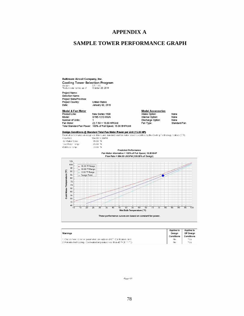
78
APPENDIX A
SAMPLE TOWER PERFORMANCE GRAPH

79
APPENDIX B
MATLAB CODE USED FOR TOWER PERFORMANCE
PREDICTION
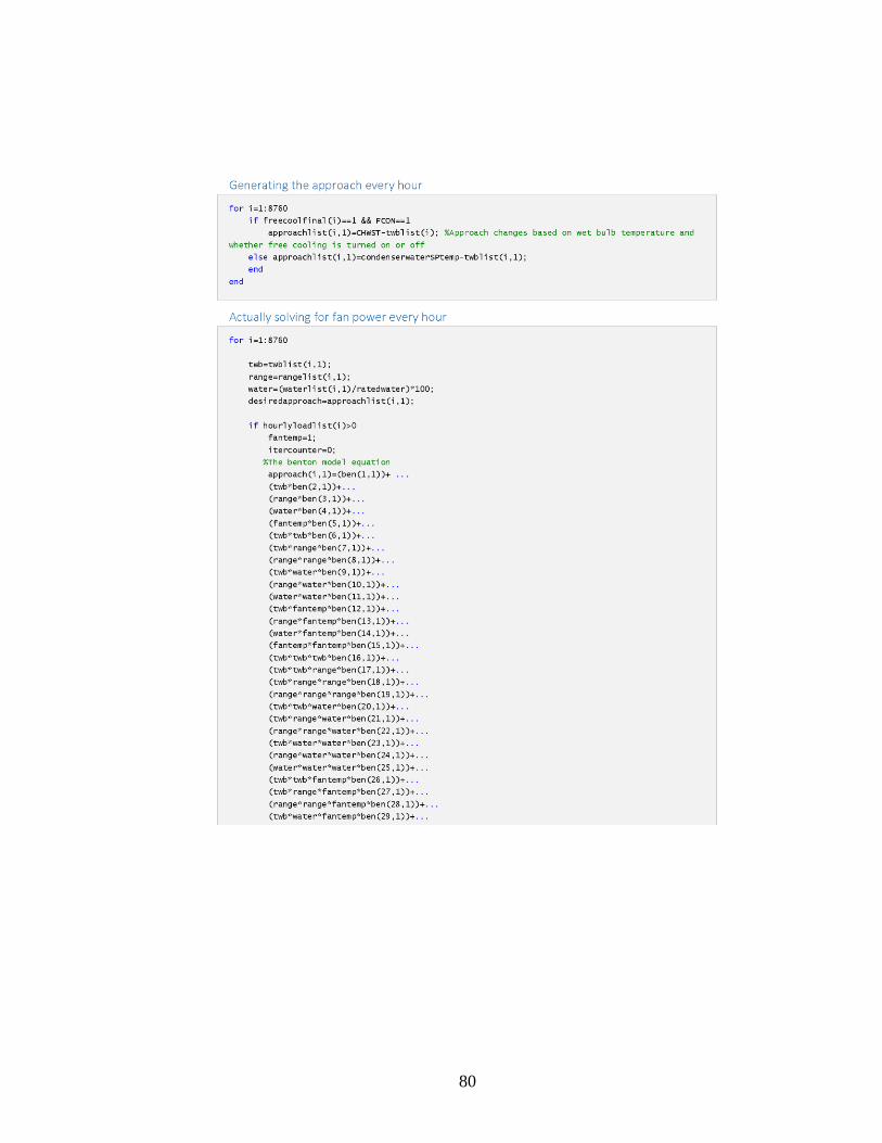
80

81

82
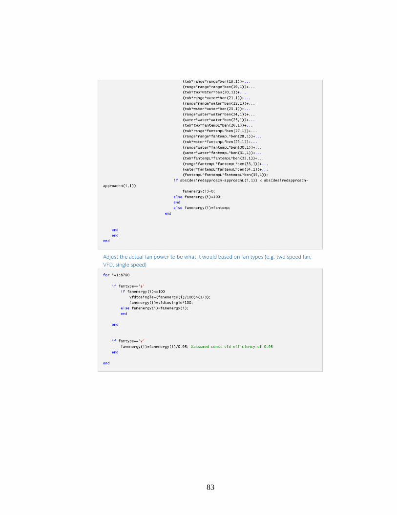
83

84
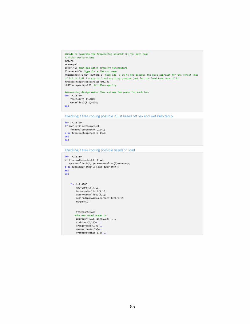
85

86
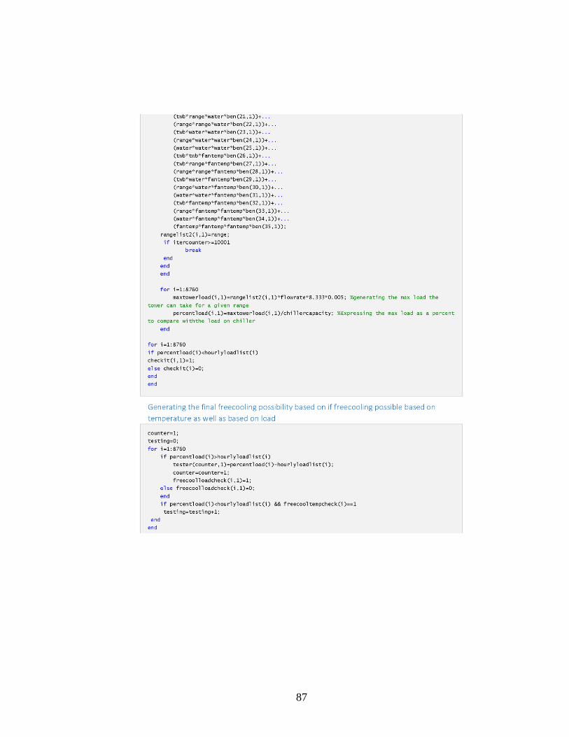
87

88

89
REFERENCES
[1] Saidur, R., Abdelaziz, E., Hasanuzzaman, M., 2010, "A Study of Energy Efficiency,
Economic and Environmental Benefits of a Cooling Tower," International Journal of
Mechanical and Materials Engineering, 5(1) pp. 87-94.
[2] Benton, D. J., Bowman, C. F., Hydeman, M., 2002, "An Improved Cooling Tower
Algorithm for the CoolToolsTM Simulation Model," ASHRAE Transactions, 108.
[3] Elovitz, K. M., 1994, "Can Your Plant Benefit from Free Cooling?" Plant
Engineering, 48(5) pp. 76-78.
[4] Mulyandasari, V., 2011, "Cooling Tower Selection and Sizing (Engineering Design
Guideline)," KLM Technology Group.
[5] Stanford, H.W., 2012, "HVAC Water Chillers and Cooling Towers: Fundamentals,
Application, and Operation," CRC Press.
[6] Hill, G.B., Pring, E., and Osborn, P.D., 1990, "Cooling Towers: Principles and
Practice," Butterworth-Heinemann.
[7] Merkel, F., 1925, "Verdunstungskühlung," Verein Deutscher Ingenieure Verlag.
[8] Kloppers, J. C., and Kröger, D., 2005, "A Critical Investigation into the Heat and
Mass Transfer Analysis of Counterflow Wet-Cooling Towers," International Journal of
Heat and Mass Transfer, 48(3) pp. 765-777.
[9] Baker, D. R., and Shryock, H. A., 1961, "A Comprehensive Approach to the Analysis
of Cooling Tower Performance," Journal of Heat Transfer, 83(3) pp. 339-349.
[10] Bourillot, C., 1983, "TEFERI: Numerical model for calculating the performance of
an evaporative cooling tower," Electricite de France, 78-Chatou. Thermal Transfer and
Aerodynamic Dept.
[11] Benton, D.J., 1983, "A numerical simulation of heat transfer in evaporative cooling
towers," Tennessee Valley Authority, WR28-1-900-110.

90
[12] Majumdar, A., Singhal, A., and Spalding, D., 1983, "Numerical Modeling of Wet
Cooling towers—Part 1: Mathematical and Physical Models," Journal of Heat Transfer,
105(4) pp. 728-735.
[13] Jaber, H., and Webb, R., 1989, "Design of Cooling Towers by the Effectiveness-
NTU Method," Journal of Heat Transfer, 111(4) pp. 837-843.
[14] Bergsten, B., 2009, "Evaporative Cooling Tower and Chilled Beams. Design
Aspects for Cooling in Office Buildings in Northern Europe." Institutionen För Energi
Och Miljö, Installationsteknik, Chalmers Tekniska Högskola, pp. 978-991.
[15] Poppe, M., and Rögener, H., 1991, "Berechnung Von Rückkühlwerken," VDI
Wärmeatlas, Pp.Mi.
[16] Kloppers, J., and Kröger, D., 2004, "Cooling Tower Performance: A Critical
Evaluation of the Merkel Assumptions," R&D Journal.
[17] Al-Waked, R., and Behnia, M., 2006, "CFD Simulation of Wet Cooling Towers,"
Applied Thermal Engineering, 26(4) pp. 382-395.
[18] Hajidavalloo, E., Shakeri, R., and Mehrabian, M. A., 2010, "Thermal Performance
of Cross Flow Cooling Towers in Variable Wet Bulb Temperature," Energy Conversion
and Management, 51(6) pp. 1298-1303.
[19] Baltimore Air Coil Technical Resources, 2012, "Minimizing Energy Costs with Free
Cooling," Baltimore Air Coil.
[20] Forrester, A. I., and Keane, A. J., 2009, "Recent Advances in Surrogate-Based
Optimization," Progress in Aerospace Sciences, 45(1) pp. 50-79.
[21] Koziel, S., Ciaurri, D.E., and Leifsson, L., 2011, "Computational Optimization,
Methods and Algorithms,"Springer, pp. 33-59.
[22] Queipo, N. V., Haftka, R. T., Shyy, W., 2005, "Surrogate-Based Analysis and
Optimization," Progress in Aerospace Sciences, 41(1) pp. 1-28.
[23] Gershenson, C., 2003, "Artificial Neural Networks for Beginners," ArXiv Preprint
cs/0308031.

91
[24] Kramer, O., 2013, "Dimensionality Reduction with Unsupervised Nearest
Neighbors,"Springer, pp. 18, Chap. 2.5.
[25] Olson, D.L., and Delen, D., 2008, "Advanced Data Mining Techniques,"Springer
Science & Business Media, pp. 141.
[26] Zhu, X., 2007, "Knowledge Discovery and Data Mining: Challenges and Realities:
Challenges and Realities,"Igi Global, pp. 249.
[27] Jin, R., Chen, W., and Simpson, T. W., 2001, "Comparative Studies of
Metamodelling Techniques Under Multiple Modelling Criteria," Structural and
Multidisciplinary Optimization, 23(1) pp. 1-13.