crash models for rural intersections: four-lane by two ... · crash models for rural intersections:...
TRANSCRIPT

Crash Models for Rural Intersections:
Four-Lane by Two-Lane
Stop-Controlled and Two-Lane by
Two-Lane Signalized
PUBLICATION NO. FHWA-RD-99-128 OCTOBER 1999
u.sw~rtment ofTmnsportationWdeml HigWay Administmtion
Research, Development, and TechnologyTurner-Fairbank Highway Research Center6300 Georgetown PikeMcLean, VA 22101-2296

This report provides direct input into the Accident Analysis Module (AAM) of the InteractiveHighway Safety Design Model. The AAM is a tool that highway engineers can use to evaluatethe impacts of highway design elements in project planning and preliminary design. Three crashmodels were developed relating crashes to three types of rural intersections. These types are: (1)three-legged intersections with major four-lane roads and minor two-lane roads that are stop-controlled, (2) four-legged intersections with major four-lane roads and minor two-lane roadsthat are stop-controlled, md (3) signalized intersections with both major and minor two-laneroads.
Elaborate sets of data were acquired from State data sorsrces (Michigan and California) andcollected in the field. The final data sets consist of 84 sites of the three-legged intersections, 72sites of the four-legged intersections, and 49 sites of the signalized intersections. Negativebinomial models — variants of Poisson models that allow for overdispersion — were developedfor each of the three data sets. Significant variables included major and minor road traffic; peakmajor and minor lefi-tum percentage; peak truck percentage; number of driveways; andchaunelization, intersection median widths, vertical alignment, and, in the case of signalizedintersections, the presence or absence of protected left-turn phases. Separate models weredeveloped for crashes resulting in injuries and total crashes.
Michael F. “TrentacosteDirector, Office of Safety
Research and Development
NOTICE
This document is disseminated rmder the sponsorship of the Department of Transportation in theinterest of information exchange. The United States Government assumes no liabihty for itscontent or use thereof The report does not constitute a standard, specification, or regulation.
The United States Government does not endorse products or manufacturers. Trade andmanufacturers’ names appear in this report only because they are considered essential to theobject of the document.
-.. , . . . .. . .. ... .. ..., CC,,,,,c, i ,<cp”r, ““cuf,,cflca,r”r, ,z#
,. ..,.,,.,., 2. Gove,. mc!lt ,.c.cssio” N.. 3. ,,c,,,,,,, rt C,,,, ”g ,..
FHWA-RD.99-I284.m,,.1!,,sub,,,,, ,, s?,,.,,,,;,,.
CRASHMODELSFOR RURAL INTERSECTIONS: FOUR-LANE BY October 1999TWO-LANE STOP-CONTROLLED AND TWO-LANE BY TWO- 6.,,.,”,,,>,,7,<,,.,>7?<.,,08> <:.<,,
LANE SIGNALIZED
7. ..,,.,(s) 8. PC,f,,,r!,,,!, (1,,,,, !,>.:,,,.,) )1.,,,,,, s!,.
AndrewVogt9.,,,f.,mC,,?0,,,”..,;.”N,,,,,.,,,,,,,<,<,,.s, !0.\\,.,,u.), NO.(Tr<,.)s,
Pragmatic, Inc. 3A5A7926 Jones Branch Drive, Suite 711 ,,. c.,?,..,, ., c,,!!, .,.,McLean, Virginia 22102 DTFH61 -96-C-00076
1,,S,>.,,s.rt”gA,.,,<,,.!,,. ,,.d.,,,,,s ,3.7,),, .,,,,,.,, ,!!>,,<,,0<!co.,,,!,
Final ReportOffice of Safety R&DFederal Highway Administration
Septembel- 1996- May 1999
6300 Georgetown Pike,4.S,)”lls”rl!?,,,,,!1,,Cud,
McLean, Virginia 22101-2296
,,, S.pp,e,,.,,ta,y,,.,,$
Contacting Officer’s Tech,,ical Representative (COTR): Joe G. Bared, HRDS
,6.,,,5,,,.,
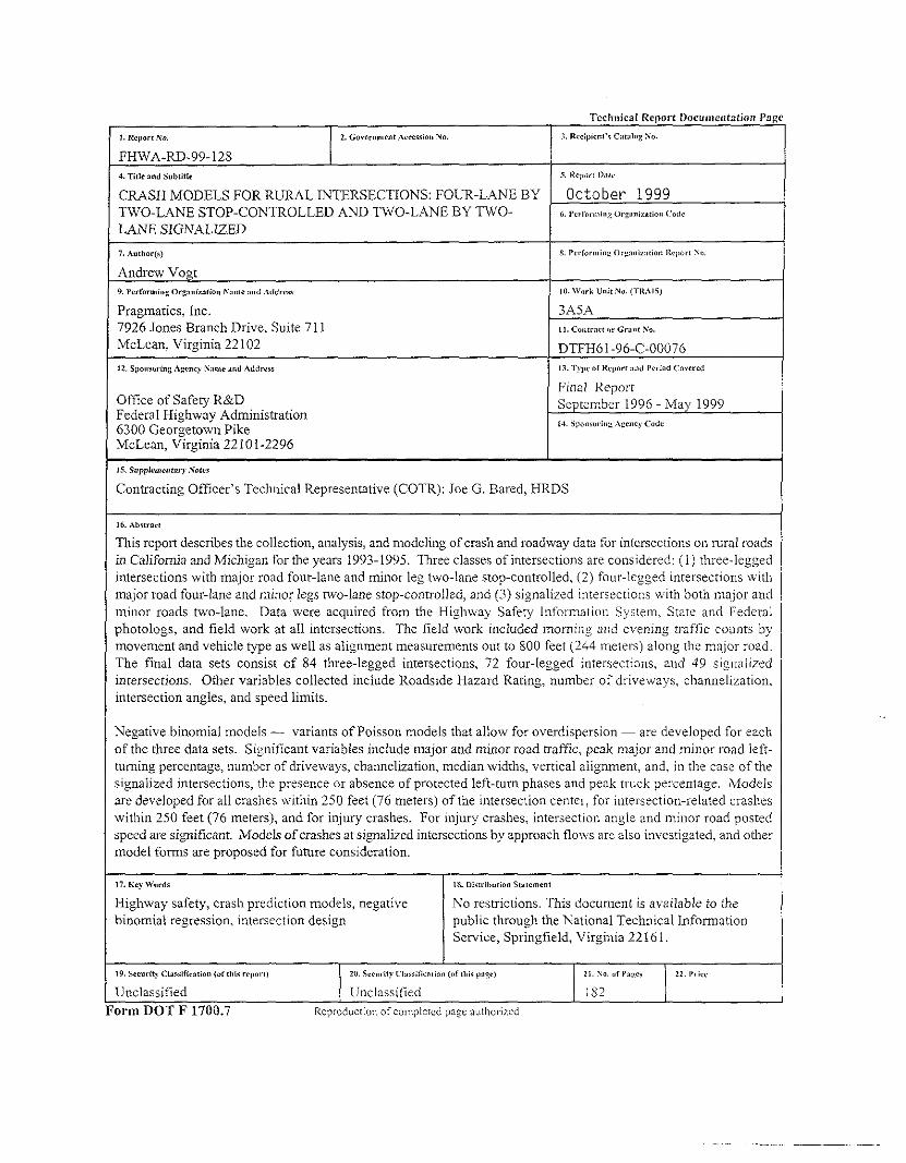
This repofi describes the collection, analysis, and nlodeling of crash and roadway data for intersections OL1l~lral roadsin California and Michigan for the years 1993-1995. Three classes of intersections are col]side red: ( 1) three-leggedintersections with major road four-lane and miller leg two-lane stop-controlled, (2) foL!r-legged intersections ~vith
major road four-larle and rllinor legs ~o-lane stop-controlled, al]d (3) signalized intersections with both major and[nillox roads two-lane, Data were acquired from the Highway Safety Iljforl]la[ioll Systelll, Svate and Federal
?hotologs, and field work at all intersections. The field work included morni!lg a,lcl evening t]-nffic cou]]ts bymovement and vehicle type as well as alignment measurements out to 800 feet (244 Lnetels) along Ibe majol- road.rhe final data sets consist of 84 three-legged intersections, 72 four-legged intersections, and 49 sig[,;! Iizedintersections. Other vuiables collected inchlde Roadside Hazard Rating, ntlmber of driveways, channelization,intersection angles, and speed limits.
Negative binomial models — variants of Poisson models that allow for ovcrdispersion — are developed for each
>f the three data sets. Sigtlificant variables include tnajor and minor road traffic, peak major and mi]]or road left-:uming percentage, Ilumber of drive~vays, challnelization, Inedian \vidths, vertical ali2nment, and, ill the case of thesignalized intcl-sections, the presence or absence of protected left-turn phases and peak trllck percentage. Models%redeveloped for all crashes n,ithin 2j0 feet (76 meters) of the intersection center, fo~ intersection-related crasheswithin 250 feet (76 meters), and for inju~ crashes. For injury crashes, intersection an~le and nlillor L-oadposted
;peed are significant. Models of crashes at signalized intersections by approach flows are also investigated, al~d othermodel fores are proposed for futire consideration.
,,. Kc)word, ,,. m,,r,b.,,.. s,,,,.,.,
Highway safety, crash prediction models, negative No reswictions. This docunlent is available to thexinomial regression, intersection design public through the National Technical Information
Sewice, Springfield, Virginia22161.
,,, s,,”!!,,C,.,,,”.,,,.. {“,,,,is,<,”,,, ,,. s,,,,,,,, .,.,,,,,.,,, ”,, {(,( ,,,,, ,,.,,) ,,, . . . “f ,.,,, ,2, ,,.,,<
Unclassified Unclassified 18?..—.nam n .-.. . .,. ,., ,,.,1-1,, ““ k r , ,“”. , Kcpro””c,!”n or c“,mplerc” pogc ,Llll,or)z,”

ACKNOWLEDGMENTS
At the direction of FH WA, the word “crasN’ and its variants have been substituted for “accident”md its variants except in special contexts.
The author expresses appreciation to staff members of the Federal Highway Administration’sTumer-Fairbank Highway Research Center (especially Dr. Joe Bared), the Highway SafetyInformation System, the California and Michigan Departments of Transportation, and Pragmatic,Inc. (especially Highway Engineer Jian Song). ThdnIcs aisoto Ezra Hauer, [o Tinl Neuman andKevin Slack of CH2M HILL, md to engineering students at Sacramento State, Michigan State, andLansing Community College.
ii

APPROXIMATECONVERSIONS TO S1 UNITS APPROXIMATE CONVERSIONSFROMS1 UNITS
:ymbol WhenYou Know MultlplyBy To Find Symbol Symbol When You Know Multlply By To Find Symbo
LENGTH LENGTH
Inches 25,4
feet 0.W5y~ds 0,914
miles !,s1
milbmetersmetersmete,,kilomoler~
mmmmkm
mm,~,~,
hakm,
mLL~,~,
Qk9MQ(or ,1.)
~c
lx.tim*
NkPa
mill(mators 0,039 Inchesmeters 3,28 lootmeters 1,m yard~tilomelers 0,621 miles
Inkydml
IntntysECmi$
R02galwy@
02
inhydmi
mmm
Fm
mm>~,~t
hakm*
mLLm>~,
Q.kQMQ(or .1.)
~c
lx&m,
NtPa
AREA AREA
squwe inchas 6&.26qu3m feet 0,W3Sqm yti$ 0,636aua$ 0,405squua miles 2.59
square millimotorssquaro meterssquare metershecwessquare tilome!ers
0,~1610,7M1,1952,470,M6
VOLUME
0.N40,26435,71f,m7
squara Inchessquare 19%1square ywd%awessquaro miles
VOLUME
miltilitorsli{erscubic meterscubic reelers
n02galwy@
fluid oun~s 29.67QdlOnS 3,?85cutic feet 0,028cubic yards 0,765
fluld ounwsgallonsCubb footcubic y~d s
NOTE: Volumes groster tianlWO lshallbshownin m’.
MASS
ounms 28.35
: pounds 0.454
T shot Ions (%W lb) 0.M7
MASS
grams 0,035tilogmms 2.82mWaQrams 1,103l., .mottic IOn.)
gramskilogramsm%agr.ms(or .mol,ic ton.)
pounds lb6hofllon$(~~\b) T
TEMPERATURE(exact)
‘F Fahrenheit 5(F-32)/9
temmmtim or (F-32)/f.8
TEMPERATURE(exact)
Colclus 1,8C +32 Fahmnhelf *Flompraum lemwraturo
lLLUMINNrlON
1.X O,wm foot~ndles fccan<im> o.m19 Ioof-bmkm O
FORCE and PRESSUREor STRESS
newtons 0,225ti10p8$a1$
pound form Ibf0,145 ! oound form mr Ibfhni
ILLUMINATION
fc Iootendles 10,76
fl loot.bmbm 3,426
FORCE and PRESSURE or STRESS
Ibf pound form 4,45 netiom
lhffin, poudfwm Wr 6,8% kilopa$alss~are Inch
—
(Reti$ed &p@mMr iW3)
.squ~a inch
118the symbl h tie In!emadond Sys!em of Units, Approprla!erounding should be mab to ~mply wi!h Smdon 4 of ASTM E3s0.
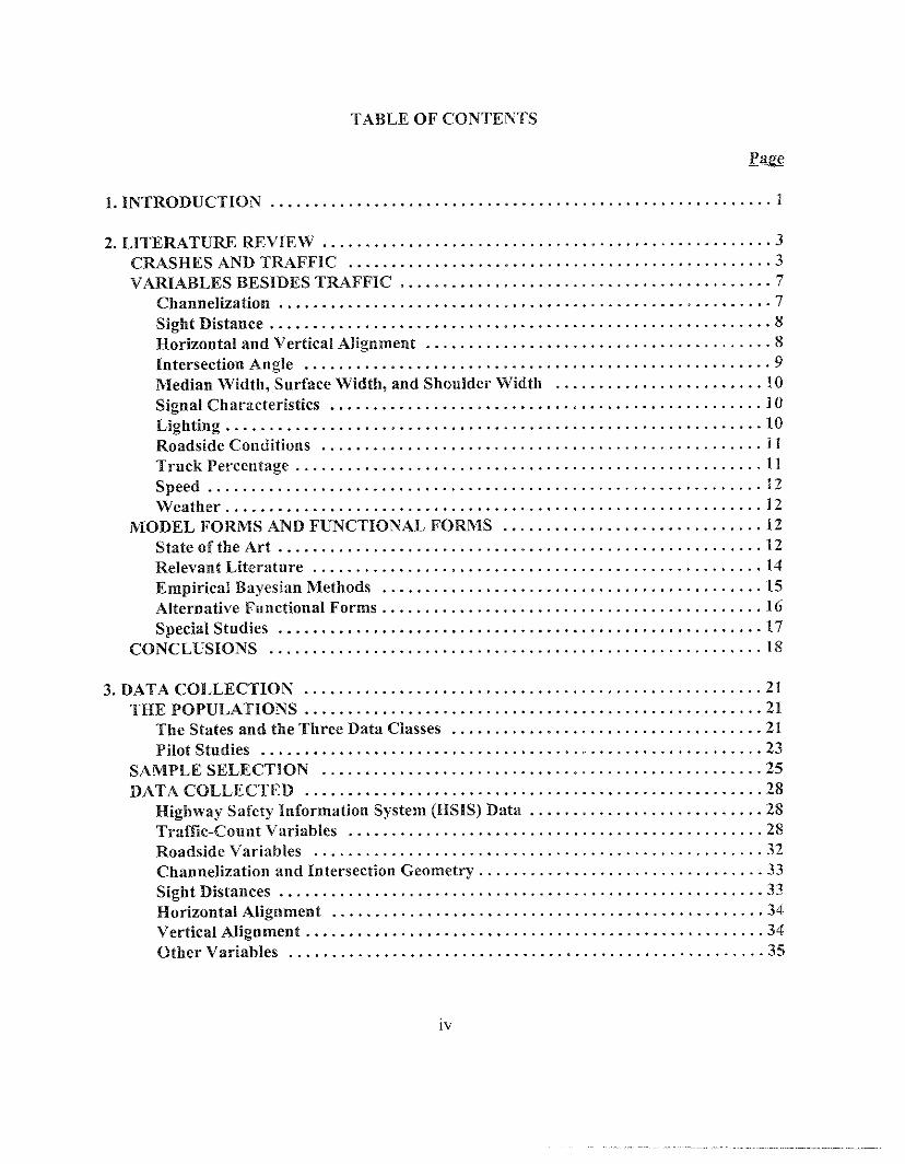
TABLE OF CONTENTS
1. INTRODUCTION . . . . . . . . . . . . . . . . . . . . . . . . . . . . . . . . . . . . . . . . . . . . . . . . . . . . . . . . . . 1
2. LITE~TU~ R.EVIEW 3. . . . . . . . . . . . . . . . . . . . . . . . . . . . . . . . . . . . . . . . . . . . . . . . . . . . .
CMSHES AND TWFFIC . . . . . . . . . . . . . . . . . . . . . . . . . . . . . . . . . . . . . . . . . . . . . . . . . 3
VARIABLES BESIDES TWFFIC.. . . . . . . . . . . . . . . . . . . . . . . . . . . . . . . . . . . . . . . ...7Channelization . . . . . . . . . . . . . . . . . . . . . . . . . . . . . . . . . . . . . . . . . . . . . . . . . . . . . . . . . 7
Sight Distance . . . . . . . . . . . . . . . . . . . . . . . . . . . . . . . . . . . . . . . . . . . . . . . . . . . . . . . . . . 8
Horizontal and Vertical Alignment . . . . . . . . . . . . . . . . . . . . . . . . . . . . . . . . . . . . . . . . 8
Intersection Angle . . . . . . . . . . . . . . . . . . . . . . . . . . . . . . . . . . . . . . . . . . . . . . . . . . . ...9Median Widthj Surface Width, and Shoulder Width . . . . . . . . . . . . . . . . . . . . . . . . 10
Signal Characteristics . . . . . . . . . . . . . . . . . . . . . . . . . . . . . . . . . . . . . . . . . . . . . . . . . . 10
Lighting . . . . . . . . . . . . . . . . . . . . . . . . . . . . . . . . . . . . . . . . . . . . . . . . . . . . . . . . . . . . . . 10
Roadside Conditions . . . . . . . . . . . . . . . . . . . . . . . . . . . . . . . . . . . . . . . . . . . . . . . . . . . 11
Truck Percentage . . . . . . . . . . . . . . . . . . . . . . . . . . . . . . . . . . . . . . . . . . . . . . . . . . . ...11Speed . . . . . . . .. . . . . . . . . . . . . . . . . . . . . . . . . . . . . . . . . . . . . . . . . . . . . . . . . . . . . . ..?2Weather . . . . . . . . . . . . . . . . . . . . . . . . . . . . . . . . . . . . . . . . . . . . . . . . . . . . . . . . . . . ...12
MODEL FORMS AND FUNCTIONAL FOmS . . . . . . . . . . . . . . . . . . . . . . . . . . . ...12
State of the Art . . . . . . . . . . . . . . . . . . . . . . . . . . . . . . . . . . . . . . . . . . . . . . . . . . . . . . . . 12
Relevant Literature . . . . . . . . . . . . . . . . . . . . . . . . . . . . . . . . . . . . . . . . . . . . . . . . . ...14Empirical Ba~esian Methods . . . . . . . . . . . . . . . . . . . . . . . . . . . . . . . . . . . . . . . . . . . . 15
Alternative Functional Forms... . . . . . . . . . . . . . . . . . . . . . . . . . . . . . . . . . . . . . . ...16Special Studies . . . . . . . . . . . . . . . . . . . . . . . . . . . . . . . . . . . . . . . . . . . . . . . . . . . . . . . . 17
CONCLUSIONS . . . . . . . . . . . . . . . . . . . . . . . . . . . . . . . . . . . . . . . . . . . . . . . . . . . . . . . . . 1$
3. DATA COLLECTION . . . . . . . . . . . . . . . . . . . . . . . . . . . . . . . . . . . . . . . . . . . . . . . . . . . . . 21
THE POPULATIONS . . . . . . . . . . . . . . . . . . . . . . . . . . . . . . . . . . . . . . . . . . . . . . . . . . ...21The States and the Three Data Classes . . . . . . . . . . . . . . . . . . . . . . . . . . . . . . . . . . . . 21
Pilot Studies . . . . . . . . . . . . . . . . . . . . . . . . . . . . . . . . . . . . . . . . . . . . . . . . . . . . . . . . . 23
SAMPLE SELECTION . . . . . . . . . . . . . . . . . . . . . . . . . . . . . . . . . . . . . . . . . . . . . . . . ...25DATA COLLECTED . . . . . . . . . . . . . . . . . . . . . . . . . . . . . . . . . . . . . . . . . . . . . . . . . . . . . 28
Highway Safety Information System (HSIS) Data . . . . . . . . . . . . . . . . . . . . . . . . . ..2STraffic-Count Variables . . . . . . . . . . . . . . . . . . . . . . . . . . . . . . . . . . . . . . . . . . . . . . . . 2s
Roadside Vari>lbles 32. . . . . . . . . . . . . . . . . . . . . . . . . . . . . . . . . . . . . . . . . . . . . . . . . . . .Channelization and Intersection Geometry . . . . . . . . . . . . . . . . . . . . . . . . . . . . . . . ..33
Sight Distances 33. . . . . . . . . . . . . . . . . . . . . . . . . . . . . . . . . . . . . . . . . . . . . . . . . . . . . . . . .Horizontal Alignment . . . . . . . . . . . . . . . . . . . . . . . . . . . . . . . . . . . . . . . . . . . . . . . . . . 34
Vertical Alignment . . . . . . . . . . . . . . . . . . . . . . . . . . . . . . . . . . . . . . . . . . . . . . . . . . . ..34iOther Variables . . . . . . . . . . . . . . . . . . . . . . . . . . . . . . . . . . . . . . . . . . . . . . . . . . . . ...35
iv

TABLEOFCONTENTS(continued)
m
DATA LIMITATIONS . . . . . . . . . . . . . . . . . . . . . . . . . . . . . . . . . . . . . . . . . . . . . . . . . ...35HSIS Data . . . . . . . . . . . . . . . . . . . . . . . . . . . . . . . . . . . . . . . . . . . . . . . . . . . . . . . ...35Field Data . . . . . . . . . . . . . . . . . . . . . . . . . . . . . . . . . . . . . . . . . . . . . . . . . . . . . . . . . . . . 35
4. ANALYSIS . . . . . . . . . . . . . . . . . . . . . . . . . . . . . . . . . . . . . . . . . . . . . . . . . . . . . . . . . . . . . . . 39
NEW VARIABLES 39. . . . . . . . . . . . . . . . . . . . . . . . . . . . . . . . . . . . . . . . . . . . . . . . . . . . . . . .Crash Variables . . 39. . . . . . . . . . . . . . . . . . . . . . . . . . . . . . . . . . . . . . . . . . . . . . . . . . . . . .ADTVariables . . . . . . . . . . . . . . . . . . . . . . . . . . . . . . . . . . . . . . . . . . . . . ..........41Variables Derived From Traffic Counts . . . . . . . . . . . . . . . . . . . . . . . . . . . . . . . . . . . 42Intersection Angle Variables . . . . . . . . . . . . . . . . . . . . . . . . . . . . . . . . . . . . . . . . . . . . . 45
Sight Distances . . . . . . . . . . . . . . . . . ... . . . . . . . . . . . . . . . . . . . . . . . . . . . . . . . . . . ...48Horizontal Alignment . . . . . . . . . . . . . . . . . . . . . . . . . . . . . . . . . . . . . . . . . . . . . . . ...49Vertical Alig]l ment . . . . . . . . . . . . . . . . . . . . . . . . . . . . . . . . . . . . . . . . . . . . . . . . . . . . . 49Miscellaneous Variables . . . . . . . . . . . . . . . . . . . . . . . . . . . . . . . . . . . . . . . . . . . . . . ..5l
UNIVAWATE STATISTICS . . . . . . . . . . . . . . . . . . . . . . . . . . . . . . . . . . . . . . . . . . . . . . . 52
Crash Data Versus Intersection C1ass and State . . . . . . . . . . . . . . . . . . . . . . . . . . . . 65BIVANATE STATISTICS . . . . . . . . . . . . . . . . . . . . . . . . . . . . . . . . . . . . . . . . . . . . . . . 67
Crashes Versus Other Variables . . . . . . . . . . . . . . . . . . . . . . . . . . . . . . . . . . . . . . . ..67
ADT and State Versus Other Variables . . . . . . . . . . . . . . . . . . . . . . . . . . . . . . . . . . . .76Correlations Betlveen Intersection Variables . . . . . . . . . . . . . . . . . . . . . . . . . . . . . . . 85Correlations for Single-Vehicle and Mu!tiple-Vehicle Crashes at Signalized
Intersections . . . . . . . . . . . . . . . . . . . . . . . . . . . . . . . . . . . . . . . . . . . . . . . . . . . . . . ...90Turning Percentage Variables . . . . . . . . . . . . . . . . . . . . . . . . . . . . . . . . . . . . . . . . ...90Crashes Verses ADT.. . . . . . . . . . . . . . . . . . . . . . . . . . . . . . . . . . . . . . . . . . . . . . . . . . . 96.4.M. Versus P.M. Truck Percentages . . . . . . . . . . . . . . . . . . . . . . . . . . . . . . . . . . . . 101
CONCLUSIONS . . . . . . . . . . . . . . . . . . . . . . . . . . . . . . . . . . . . . . . . . . . . . . . . . . . . . . . . 101
5. MODELING . . . . . . . . . . . . . . . . . . . . . . . . . . . . . . . . . . . . . . . . . . . . . . . . . . . . . . . . . . . . . 105THEORY . . . . . . . . . . . . . . . . . . . . . . . . . . . . . . . . . . . . . . . . . . . . . . . . . . . . . . . . . . . . . . 105
Modeling . . . . . . . . . . . . . . . . . . . . . . . . . . . . . . . . . . . . . . . . . . . . . . . . . ...........~~5P-Values and Goodness of Fit . . . . . . . . . . . . . . . . . . . . . . . . . . . . . . . . . . . . . . . . . . . 107
Model Building . . . . . . . . . . . . . . . . . . . . . . . . . . . . . . . . . . . . . . . . . . . . . . . . . . . . . . . 110
MODELS FOR TH~E-LEGGED INTERSECT~~NS . . . . . . . . . . . . . . . . . . . . . . ..~l~MODELS FOR FOUR-LEGGED INTERSECTIONS . . . . . . . . . . . . . . . . . . . . . . . . . 115
MODELS FOR TI-IE SIGNALIZED INTERSECTIONS . . . . . . . . . . . . . . . . . . . . . ..120Negative Binomial Models . . . . . . . . . . . . . . . . . . . . . . . . . . . . . . . . . . . . . .........~2QFlow Models . . . . . . . . . . . . . . . . . . . . . . . . . . . . . . . . . . . . . . . . . . . . . . . . . . . . . . . . . 126
RESIDUAL ANALYSIS . . . . . . . . . . . . . . . . . . . . . . . . . . . . . . . . . . . . . . . . . . . . . . . . . . 129
v

TABLE OF CONTENTS(continued)
6. CONCLUSIONS . . . . . . . . . . . . . . . . . . . . . . . . . . . . . . . . . . . . . . . . . . . . . . . . . . . . . . . ..l45THE MAIN MODELS . . . . . . . . . . . . . . . . . . . . . . . . . . . . . . . . . . . . . . . . . . . . . . . . . ...145
Three-Legged Intersections . . . . . . . . . . . . . . . . . . . . . . . . . . . . . . . . . . . . . . . . . . ...145Four-Legged Intersections . . . . . . . . . . . . . . . . . . . . . . . . . . . . . . . . . . . . . . . . . . ...147Signalized Intersections . . . . . . . . . . . . . . . . . . . . . . . . . . . . . . . . . . . . . . . . . . . . . . . . 149
EXPLANATORY VALUE OF MAIN MODELS . . . . . . . . . . . . . . . . . . . . . . . . . . . ...151ACCIDENT ~DUCTION FACTORS . . . . . . . . . . . . . . . . . . . . . . . . . . . . . . . . . . . ...155SUMMARY . . . . . . . . . . . . . . . . . . . . . . . . . . . . . . . . . . . . . . . . . . . . . . . . . . . . . . . . . . ..~57
APPENDIX. DATA FROM PILOT STUDY PHASE OF DATA COLLECTION. . . . ...161
REFERENCES . . . . . . . . . . . . . . . . . . . . . . . . . . . . . . . . . . . . . . . . . . . . . . . . . . . . . . . . . . ...167
vi
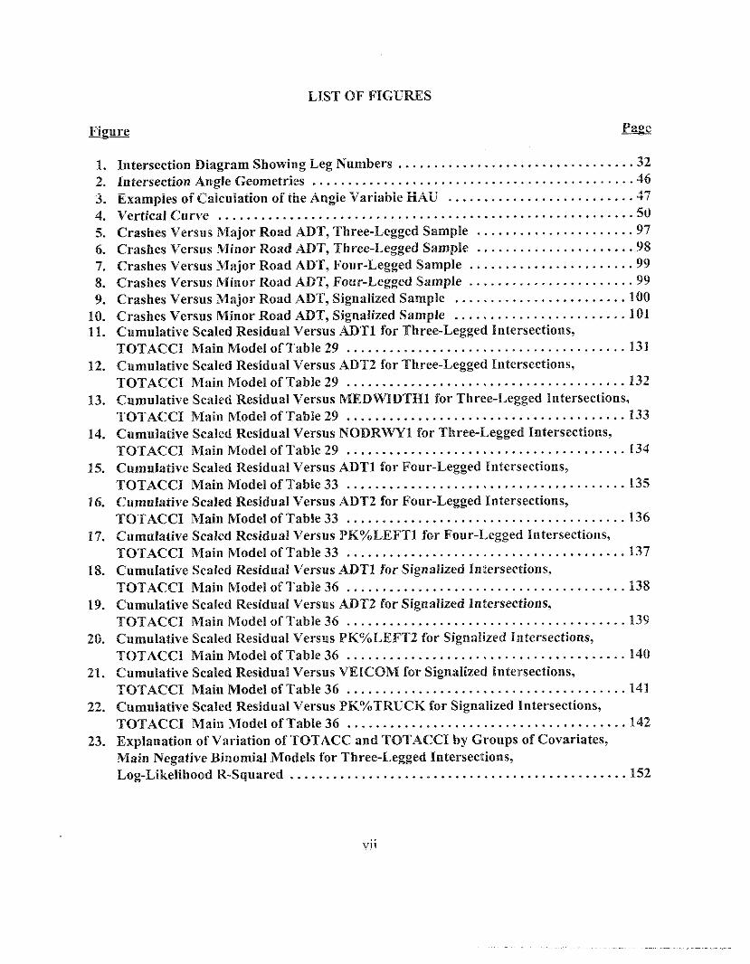
LIST OF FIGURES
1.2.3.4.5.6.7.8.9.
10.11.
12.
13.
14.
15.
16.
17.
18.
19.
20.
21.
22.
23.
Intersection Diagram ShowingLeg Numbers . . . . . . . . . . . . . . . . . . . . . . . . . . . . . . ...32Intersection Angle Geometries . . . . . . . . . . . . . . . . . . . . . . . . . . . . . . . . . . . . . . . . . . . . . 46
Examples of Calculation of the Angie Variable HAU . . . . . . . . . . . . . . . . . . . . . . . . . . 47
Vertical Curve . . . . . . . . . . . . . . . . . . . . . . . . . . . . . . . . . . . . . . . . . . . . . . . . . . . . . . . . . .5~Crashes Versns Major Road ADT, Three-Legged Sample . . . . . . . . . . . . . . . . . . . . . . 97
Crashes Versus Nlinor Road ADT, Three-Legge~ SamPIe . . . . . . . . . . . . . . . . . . . . . . 98Crashes Versus Major Road ADT, Four-Legged Sample . . . . . . . . . . . . . . . . . . . . . ..99Crashes Versns Minor Road ADT, Four-Legged Sample . . . . . . . . . . . . . . . . . . . . ...99Crashes Versus Major Road ADT, Signalized Sample . . . . . . . . . . . . . . . . . . . . . . . . 100Crashes Versus Minor Road ADT, Signalized Sample . . . . . . . . . . . . . . . . . . . . . . . . 101Cumulative Scaled Residual Versus ADT1 for Three-Legged Intersections,TOTACCI Main ModelOfTable 29. . . . . . . . . . . . . . . . . . . . . . . . . . . . . . . . . . . . ...131Cumulative Scaled Residu a[ Versus ADT2 for Three-Legged I]~tersections,TOTACCI Main Model of Table 29. . . . . . . . . . . . . . . . . . . . . . . . . . . . . . . . . . .....~3~Cumulative Scaled Residual Versus MEDWIDTH1 for Three-Legged Intersections,TOTACCI Main Model of Table 29 . . . . . . . . . . . . . . . . . . . . . . . . . . . . . . . . . . . . . . . 133Cumulative Scaled Residual Versus NODRWYI for Three-Legged Intersections,TOTACCI Main Model of Table 29 . . . . . . . . . . . . . . . . . . . . . . . . . . . . . . . . . . . . . . . 134Cumulative Scaled Residual Versns ADTI for Four-Legged Intersections,TOTACCI Main Model of Tabie 33 . . . . . . . . . . . . . . . . . . . . . . . . . . . . . . . . . . . . . . . 135Cumulative Scaled Residual Versus ADT2 for Four-Legged Intersections,TOTACCI Main Model of Table 33 . . . . . . . . . . . . . . . . . . . . . . . . . . . . . . . . . . . . . . 136Cumulative Scaled Residual Versns PKY.LEFT1 for Four-Legged Intersectiojls,TOTACCI Main Model of Table 33 . . . . . . . . . . . . . . . . . . . . . . . . . . . . . . . . . . . . . . . 137Cumulative Scaled Residual Versns .4DTI for Signalized Intersections,TOTACCI Main Model of Table 36. . . . . . . . . . . . . . . . . . . . . . . . . . . . . . . . . . . . ...138Cumulative Scaled Residual Versus ADT2 for Signalized Intersections,TOTACCI Main Model of Table 36. . . . . . . . . . . . . . . . . . . . . . . . . . . . . . . . . . . . ...139Cumulative Scaled Residual Versus PK”/.LEFT2 for Signalized Intersections,TOTACCI Main Model of Table 36. . . . . . . . . . . . . . . . . . . . . . . . . . . . . . . . . . . . ...140’Cumsslative Scaled Residual Versus VEICOM for Signalized Intersections,TOTACCI Main’Model of Tabie 36. . . . . . . . . . . . . . . . . . . . . . . . . . . . . . . . . . . . . ..~41Cumulative Scaled Residual Versus PK”ATRUCK for Signalized Intersections,TOTACCI Main ModelOf Table 36. . . . . . . . . . . . . . . . . . . . . . . . . . . . . . . . . . . . ...142Explanation of Variation of TOTACC and TOTACCI by Groups of Covariates,lMaiss Negative Biu omial Models for Three-Legged Intersections,Log-Likelihood R-Squared . . . . . . . . . . . . . . . . . . . . . . . . . . . . . . . . . . . . . . . . . . . . . . . 152
vii

LIS? OF FIGURES(conti,~ued)
24. Explanation of Variation of TOTACC and TOTACCI by Groups of Covariates,Main Negative Binomial Models for Four-Legged Intersections,Log-Likelihood R-Squared . . . . . . . . . . . . . . . . . . . . . . . . . . . . . . . . . . . . . . . . . . . . . ..l54
25. Explanation of Variation of TQTACC and TOTACCI by Groups of Covariates,Main Negative Binomial Models for Signalized Intersections,Log-Likelihood R-Squared . . . . . . . . . . . . . . . . . . . . . . . . . . . . . . . . . . . . . . . . . . . . ...155
A-1. Posted Speed Versus Operating Speed . . . . . . . . . . . . . . . . . . . . . . . . . . . . . . . . . . . . . 162
A-2. Daytime Speed Versus 24-Hour Speed . . . . . . . . . . . . . . . . . . . . . . . . . . . . . . . . . . . . . 163
A-3. Peak Truck Percentage Versus 24-Hour Truck Percentage . . . . . . . . . . . . . . . . . . . . 164A-4. Crash Locations aod Relationships at a Three-Legged Intersection . . . . . . . . . . . . . 16S
v]]]
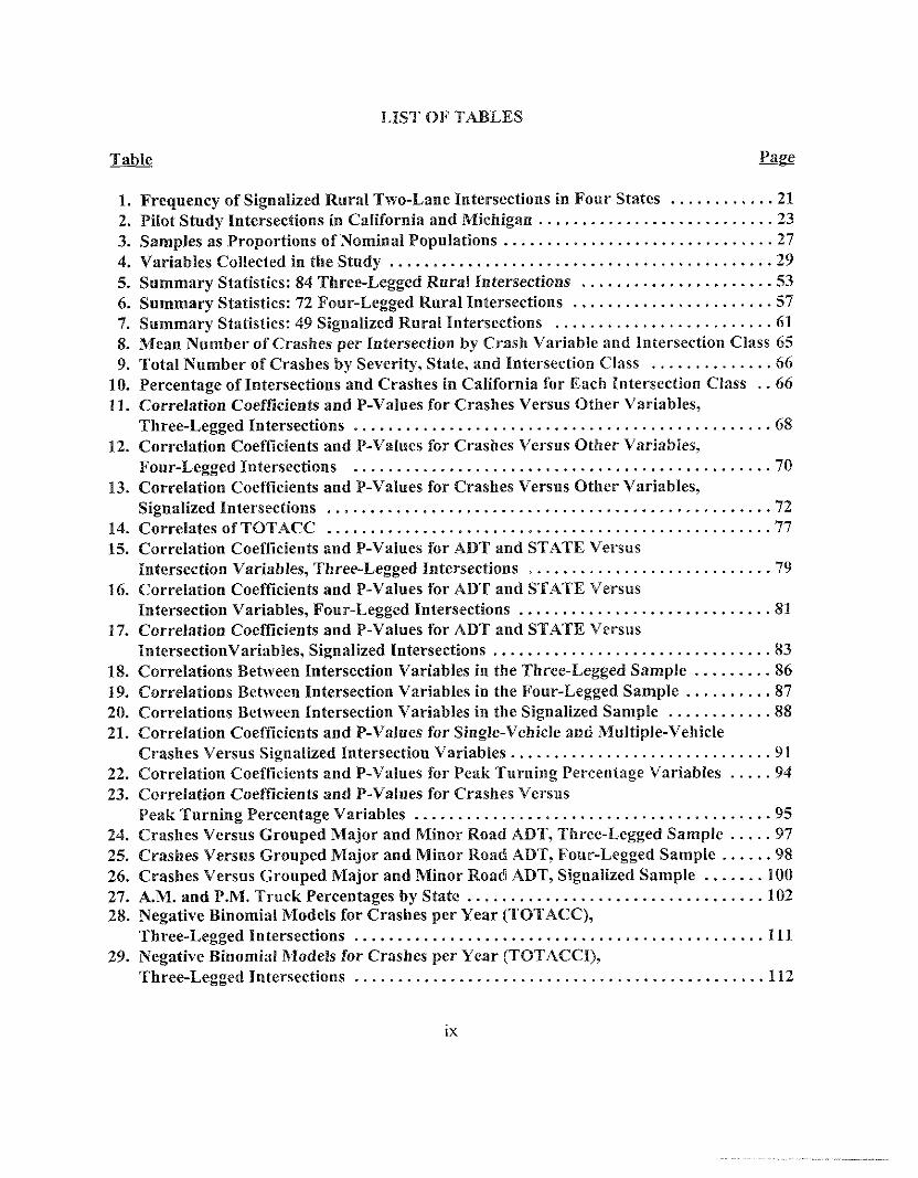
LIST OF TABLES
w &c
1. Frequency of Signalized Rural Two-Lane Intersections in Four States . . . . . . . . . ...212. Pi[ot Study Intersections in California and Michigan . . . . . . . . . . . . . . . . . . . . . . . . ...233. Samp9es as Proportions of Nominal Populations . . . . . . . . . . . . . . . . . . . . . . . . . . . . ...274. Variables Collected inthe Study. . . . . . . . . . . . . . . . . . . . . . . . . . . . . . . . . . . . . . . . . ...295. Summary Statistics: 84 Three-Legged Rural Intersections . . . . . . . . . . . . . . . . . . . ...536. Summary Statistics: 72 Four-Legged Rural Intersections . . . . . . . . . . . . . . . . . . . . . . . 577. Summary Statistics: 49 Signalized Rural Isstersections . . . . . . . . . . . . . . . . . . . . . . . . . 61
8. Mean Nu~nber of Crashes per Intersection by Crash Variable aud Intersection Class6j9. Total Number of Crashes by Severity, State, and Intersection Class . . . . . . . . . . . ...66
10. Percentage of Intersections and Crashes in California for Each Intersection Class ..6611. Correlation Coefficients and P-Valnes for Crashes Versus Otl~er Variables,
Three-Legged Intersections . . . . . . . . . . . . . . . . . . . . . . . . . . . . . . . . . . . . . . . . . . . . . . ..6$12. Correlation Coefficients and P-Values for Crasl~es Versus Other Variables,
Four-Legged Intersections . . . . . . . . . . . . . . . . . . . . . . . . . . . . . . . . . . . . . . . . . . . . . . . . 70
13. Correlation Coefficients and P-Values for Crashes Versus Other Variables,Signalized Intersections . . . . . . . . . . . . . . . . . . . . . . . . . . . . . . . . . . . . . . . . . . . . . . . . ...72
14. Correiatesof TOTACC . . . . . . . . . . . . . . . . . . . . . . . . . . . . . . . . . . . . . . . . . . . . . . . . ...7715. Correlation Coefficients and P-Values for ADTand STATE Versus
Intersection Variables, Three-Legged Intersections . . . . . . . . . . . . . . . . . . . . . . . . . . . . 7916. Correlation Coefficients and P-Values for ADTand STATE Versus
Intersection Variables, Four-Legged Intersections . . . . . . . . . . . . . . . . . . . . . . . . . . ...81
17. Correlation Coefficients and P-Values for ADTand STATE VersusIsstersectionVariables, Signalized Intersections . . . . . . . . . . . . . . . . . . . . . . . . . . . . . ...83
18. Correlations Bet\}eenI ntersectionV ariablesi lltheThree-LeggedS ample . . . . . . ...8619. Correlations Bet}veen Intersection Variables inthe Four-Legged SampIe . . . . . . . ...8720. Correlations Bet~veen Intersection Variables inthe Signalized Sample . . . . . . . . . ...8821. Correlation Coefficients and P-Values for Single-Vebicle and]Multiple-Vehicle
Crashes Versus Signalized Intersection Variables. . . . . . . . . . . . . . . . . . . . . . . . . . . ...9122. Correlation Coefficients and P-Values for Peak Tnrning Percentage Variables . . ...9423. Correlation Coefficients and P-Values for Crashes Versus
Peak Turning Percentage Variables . . . . . . . . . . . . . . . . . . . . . . . . . . . . . . . . . . . . . . ...9524. Crashes Versus Grouped Major and Minor Road ADT, Three-Legged Sample . . ...9725. Crashes Versus Grouped Major and Minor Road ADT, Four-Legged Sample . . . ...9826. Crashes Versus Grouped Major and Minor Road ADT, Signalized Sample . . . . ...10027. A.M. and P. M. Truck Percentages by State . . . . . . . . . . . . . . . . . . . . . . . . . . . . . . . ...10228. Negative Binomial Models for~rashes per Year(TOTACC),
Three-Legged Intersections . . . . . . . . . . . . . . . . . . . . . . . . . . . . . . . . . . . . . . . . . . . . . . .29. Negative Birnomiai lModels for Crashes per Year (TOTACCI),
Three-Legged Intersections . . . . . . . . . . . . . . . . . . . . . . . . . . . . . . . . . . . . . . . . . . . . . . .
ix
LIST OF TABLES(continued)
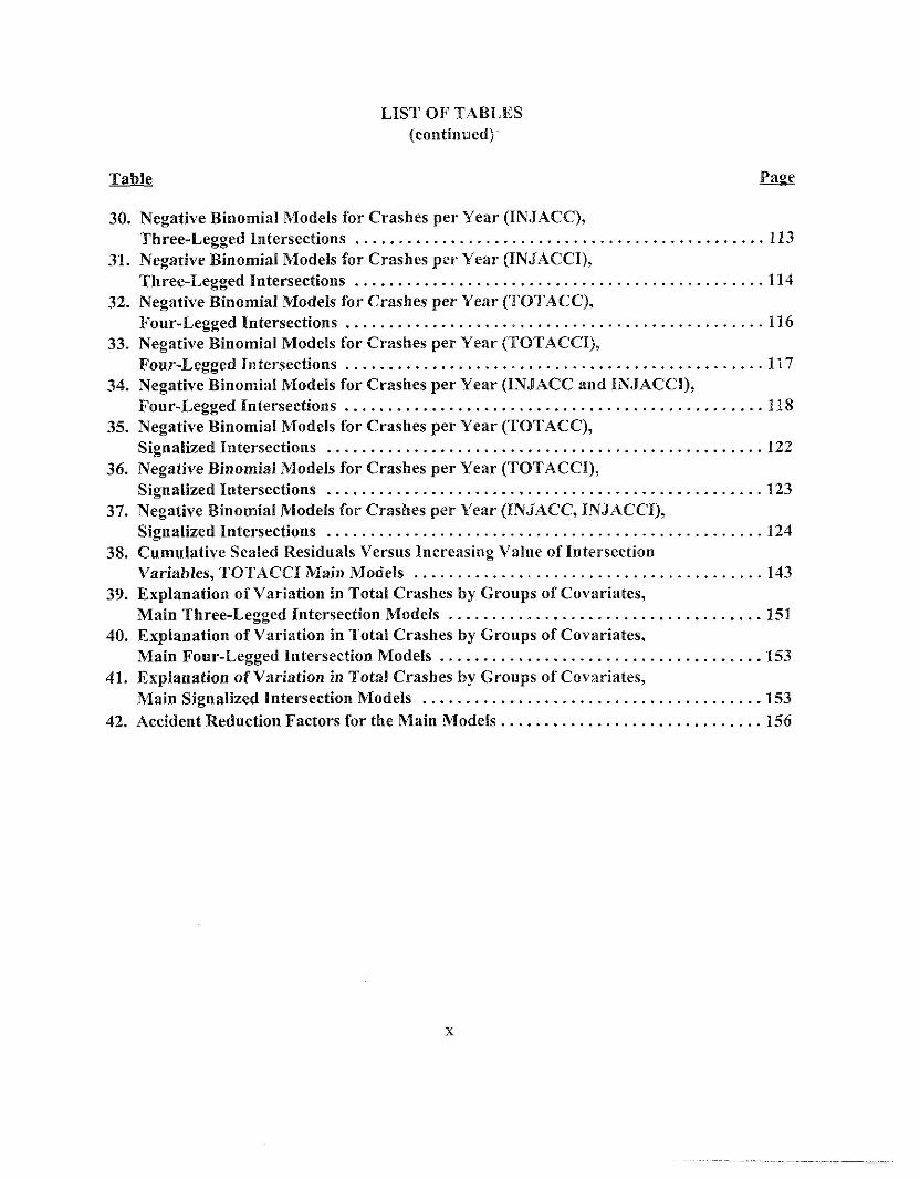
30. Negative Binomial Models for Crashes per Year (INJACC),Three-Legged Intersections . . . . . . . . . . . . . . . . . . . . . . . . . . . . . . . . . . . . . . . . . . . . ...113
31. Negative Binomial Models for Crashes per Year (INJACCI),Three-Legged Intersections . . . . . . . . . . . . . . . . . . . . . . . . . . . . . . . . . . . . . . . . . . . . ...114
32. Negative Binomial Models for Crashes per Year (TOTACC),Four-Legged Intersections . . . . . . . . . . . . . . . . . . . . . . . . . . . . . . . . . . . . . . . . . . . . . ...116
33. Negative Binomial Models for Crashes per Year (TOTACCI),Four-Leggeet intersections . . . . . . . . . . . . . . . . . . . . . . . . . . . . . . . . . . . . . . . . . . . . . ...117
34. Negative Binomial Models for Crashes per Year (INJACC and INJACCI),Four-Legged Intersections . . . . . . . . . . . . . . . . . . . . . . . . . . . . . . . . . . . . . . . . . . . . . ...118
35. Negative Binomia! Models for Crashes per Year (TOTACC),Signalized intersections . . . . . . . . . . . . . . . . . . . . . . . . . . . . . . . . . . . . . . . . . . . . . . . . . . 122
36. Negative Biuomial JModels fOr Crashes per Year (TOTACCI),Signalized Intersections . . . . . . . . . . . . . . . . . . . . . . . . . . . . . . . . . . . . . . . . . . . . . . . . . . 123
37. Negative Binomial NIodels for Crashes per l’ear (INJACC, INJACCI),Signalized Intersections . . . . . . . . . . . . . . . . . . . . . . . . . . . . . . . . . . . . . . . . . . . . . . . . . . 124
38. Cumulative Sca!ed Residuals Versus Increasing Value of IntersectionVariables, TOTACCI Main Models . . . . . . . . . . . . . . . . . . . . . . . . . . . . . . . . . . . . . . . . 143
39. Explanation of Variation in Total Crashes by Groups of Covariates,MainThree-LeggedI ntersectionModels . . . . . . . . . . . . . . . . . . . . . . . . . . . . . . . . . ...151
40. Explanation of Variation in Total Crashes by Groups of Covariates,Main Four-Legged Intersection Models . . . . . . . . . . . . . . . . . . . . . . . . . . . . . . . . . . ...153
41. Explanation of Variation in Total Crashes by Groups of Covilriates,Main Signalized Intersection Models . . . . . . . . . . . . . . . . . . . . . . . . . . . . . . . . . . . . . . . 153
42. Accident Reduction Factors forthe Main Models . . . . . . . . . . . . . . . . . . . . . . . . . . . . ..l56
x
INDEX OF VARIABLES
Variable _
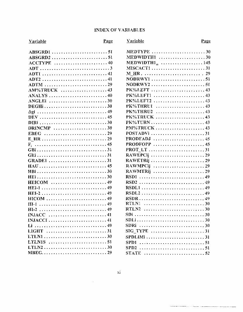
ABSG~l . . . . . . . . . . . . . . . . . . . . . . ..s1ABsGm2 . . . . . . . . . . . . . . . . . . . . . . . .51ACCTYPE . . . . . . . . . . . . . . . . . . . . ...40ACT . . . . . . . . . . . . . . . . . . . . . . . . . . . ...3ANTI . . . . . . . . . . . . . . . . . . . . . . . . . . . .41ADT2 . . . . . . . . . . . . . . . . . . . . . . . . . . . .41ADAM . . . . . . . . . . . . . . . . . . . . . . . . . . .29AM’YoTRUCK . . . . . . . . . . . . . . . . . ...43ANALYS T. . . . . . . . . . . . . . . . . . . . . . ..40ANGLEi . . . . . . . . . . . . . . . . . . . . . . ...30DEGHi . . . . . . . . . . . . . . . . . . . . . . . . . . . 30
Agi . . . . . . . . . . . . . . . . . . . . . . . . . . . ...49DEV . . . . . . . . . . . . . . . . . . . . . . . . . . ...45Dire . . . . . . . . . . . . . . . . . . . . . . . . . . . . .30DRINCMP . . . . . . . . . . . . . . . . . . . . ...30EBEG . . . . . . . . . . . . . . . . . . . . . . . . ...29E_HR . . . . . . . . . . . . . . . . . . . . . . . . . . . .29F, . . . . . . . . . . . . . . . . . . . . . . . . . . . . . ..4SGUI . . . . . . . . . . . . . . . . . . . . . . . . . . . . . .31Gee . . . . . . . . . . . . . . . . . . . . . . . . . . . . ..31GRADE1 . . . . . . . . . . . . . . . . . . . . . . . ..3 IHAU . . . . . . . . . . . . . . . . . . . . . . . . . . ...45HBi 30He: :::::::::::::::::::::::::: :::30HEICOM . . . . . . . . . . . . . . . . . . . . . ...49HEI-I . . . . . . . . . . . . . . . . . . . . . . . . . ...49HEI-2 . . . . . . . . . . . . . . . . . . . . . . . . . . . .49HICOM . . . . . . . . . . . . . . . . . . . . . . . ...49HI-1 . . . . . . . . . . . . . . . . . . . . . . . . . . ...49HI-2 . . . . . . . . . . . . . . . . . . . . . . . . . . . . .49INJACC . . . . . . . . . . . . . . . . . . . . . . ...41INJACCI . . . . . . . . . . . . . . . . . . . . . . . . .41Li d. . . . . . . . . . . . . . . . . . . . . . . . . . . . ..49LIGHT . . . . . . . . . . . . . . . . . . . . . . . ...31LTLNI . . . . . . . . . . . . . . . . . . . . . . . . . ..3OLTLNIS . . . . . . . . . . . . . . . . . . . . . . ...51LTLN2 . . . . . . . . . . . . . . . . . . . . . . . . . . .30MEG . . . . . . . . . . . . . . . . . . . . . . . . . . . .29
Variable @
NIEDTYPE . . . . . . . . . . . . . . . . . . . . . . .30MEDWIDTH1 . . . . . . . . . . . . . . . . . ...30MEDWIDTHI . . . . . . . . . . . . . . . . . . . 14sMISCACT1 . . . . . . . . . . . . . . . . . . . . . ..3 IM_HR . . . . . . . . . . . . . . . . . . . . . . . . . . 29NODRWYI . . . . . . . . . . . . . . . . . . . . . ..SINQDRWY2 . . . . . . . . . . . . . . . . . . . . . . . 51PKY”LEFT . . . . . . . . . . . . . . . . . . . . ,. .43PKYoLEFTI . . . . . . . . . . . . . . . . . . . ...43PK”h>LEFT2 . . . . . . . . . . . . . . . . . . . ...43PK%>THRU1 . . . . . . . . . . . . . . . . . . ...43PK’%,THRU2 . . . . . . . . . . . . . . . . . . ...43PK%)TRUCK . . . . . . . . . . . . . . . . . . . ..43PK”A,Tum’ . . . . . . . . . . . . . . . . . . . . ...43PMYoTRUCK . . . . . . . . . . . . . . . . . . . ..43POSTADVi . . . . . . . . . . . . . . . . . . . . . ..31PRODFADJ . . . . . . . . . . . . . . . . . . . ...45PRODFOPP . . . . . . . . . . . . . . . . . . . . . .45PROT_LT . . . . . . . . . . . . . . . . . . . . . ...31WWEPCij . . . . . . . . . . . . . . . . . . . . . ..29RAWETRij . . . . . . . . . . . . . . . . . . . . . ..29RAWMPCij . . . . . . . . . . . . . . . . . . . . . . 29WWMTRlj . . . . . . . . . . . . . . . . . . . . . . 29RSD1 . . . . . . . . . . . . . . . . . . . . . . . . . . . .49RSD2 . . . . . . . . . . . . . . . . . . . . . . . . . . . .49RSDL1 . . . . . . . . . . . . . . . . . . . . . . . . . . .49RSDL2 . . . . . . . . . . . . . . . . . . . . . . . . . . .49RSDR . . . . . . . . . . . . . . . . . . . . . . . . . . . .49RTLN1 . . . . . . . . . . . . . . . . . . . . . . . ...30RTLN2 . . . . . . . . . . . . . . . . . . . . . . . ...30sDi . . . . . . . . . . . . . . . . . . . . . . . . . . . ...30sDLi . . . . . . . . . . . . . . . . . . . . . . . . . . . ..30SDRI . . . . . . . . . . . . . . . . . . . . . . . . . ...30SIG_TYPE . . . . . . . . . . . . . . . . . . . . . . . 31
SPDLIMi . . . . . . . . . . . . . . . . . . . . . . ...31SPD1 . . . . . . . . . . . . . . . . . . . . . . . . . ...51SPD2 . . . . . . . . . . . . . . . . . . . . . . . . . . . .51STATE . . . . . . . . . . . . . . . . . . . . . . . ...52
xi

INDEX OF VARIABLES(continued)
Variable
SUMF. . .. . . . . . . . . . . . . . . . . . . . . . . . . . .45
terrain . . . . . . . . . . . . . . . . . . . . . . . . . . . 31
TOTACC . . . . . . . . . . . . . . . . . . . . . ..31~39TOTACCI . . . . . . . . . . . . . . . . . . . . . . . .:;TOTACCM . . . . . . . . . . . . . . . . . . . . . . .
TOTACCS . . . . . . . . . . . . . . . . . . . . . . .
VBi . . . . . . . . . . . . . . . . . . . . . . . . . . . . . . .VCEICOM . . . . . . . . . . . . . . . . . . . . . . ..50VCEI-1 . . . . . . . . . . . . . . . . . . . . . . . . . . 50
VCICOM . . . . . . . . . . . . . . . . . . . . . . . . . soVCI-I . . . . . . . . . . . . . . . . . . . . . . . . . . . . 50
VEH_INVOL . . . . . . . . . . . . . . . . . . . . .;;VEi . . . . . . . . . . . . . . . . . . . . . . . . . . . . . .VEICOM . . . . . . . . . . . . . . . . . . . . . . . . . 50
VEICOM . . . . . . . . . . . . . . . . . . . . . . . . 150
VEI-I . . . . . . . . . . . . . . . . . . . . . . . . . . . . 50
vi . . . . . . . . . . . . . . . . . . . . . . . . . . . . . . . 49
VICOM . . . . . . . . . . . . . . . . . . . . . . . . . . 50
VI-1 . . . . . . . . . . . . . . . . . . . . . . . . . . . . . 50
xii
1. INTRODUCTION
This study develops cmsh models for
* Rural thee-legged mdfour-leggedi ntcrsectionso nfour-lallel lighways,s top-controlledonthe minor legs.
o Signalized mral irrtersection so ftwo-laneroads
An earlier study,’ of which this maybe regarded as a continuation, treats segments of two-lane ruralroads mdmraltlwee- and four-legged intersections oftwo-lane roads, stop-controlled on the minorlegs. The two studies together consider the chief geometries on two-lane roads — segments,intersections ~vitllminor road stop-controlled, andsignalized intersect io]ls. [naddition, this studybranches out bypassing from intersections ontwo-lane roads toot3eso]l four-lane ro;lds.
A major intended use of crash models such as the ones developed here is in the Accident Analysiscomponent of the InteractiveHighwayS afetyDesignM odel(IHSDM).z The IHSDM isap]-oposedset of interactive computerprograms that will allow highway designers to examine the safetyconsequences ofvarious design alternatives. Theseprograms will assess how proposed designsrelate to driver expectations, vehicle and driver capabilities, traffic flows, and established designprinciples.
The Accident Analysis component, or Accident Analysis Module, is intended to estimate, inquantitative terns, thesafety effects -crash freque[lcies andseverities -t12at may result fromdifferent desiagns. Inaddition todrivermd vehicle variables, safety isillfltlenced bythcvolLlme andmovement of traffic. Itisalso influenced bysuchdesign features aschannelization, horizollt~\l andvertical curves, sight distances, and roadside conditions. The module was tentatively envisioned(op. cit.) to have four parts, dealing respectively with segment crashes, intersection crashes,interchange ramp crashes, and roadside crashes. The safety consequences ofa particular designwould bethesum of thecrmtribations ofeach part. Amodelwould redeveloped foreach type ofcrash andtbemodels lvouldbe cornbinedto yield an overall picture of design consequences.
‘ A. VoStand J.G. Bared, Accident MoclelsJor T>vo-La?7.eRz{/-<r[/<c)c[dx:Segrr:errts[[r?<[Intersections, Repofi No. FHWA-~-98- 133, Federal High\+,ay Administration, McLeaIl, \/a.,1998; and A. Vogt~]d J. G. Bared, c`Accident Models for Two-Lane RLiral SegmelltsatldIntersections~’ Transportation Research Record 1635: 19-29,1998.
2J.A. Reagan, “TheInteractiveH ighwayS afetyDesignModel: Designing for Safety byAnalyzing Road Geornetrics,” Pziblic Road.y: 37-43, Summer 1994.
H. Lum and J. Reagan, “Interactive Highway Safety Design Model: Accident PredictiveModule:’ FHWA Drafi 8-22-94.
1

The goal of the present study is to assess the combined and relative effects of highway vaj-iables onintersection crashes for the classes of intersections noted above. The method used, by now a well-established method, is that of genemlized linear models based on a negative binomial distribution.Crashes are thought of as discrete rare events, the number of crashes at an intersection being arandom variable of the Poisson type with overdispersion. The mean number of crashes is anexponential fLmction of a linear combination of intersection variables and the vari fince in crashcounts depends on the mean, as well as on an overdispersion parameter representing factors notincI uded in the modeI.
In Chapter 2, literature on modeling of intersection crashes is reviewed. In Chapters 3 and 4, the datacollection and preliminary analysis are described, and in Chapter 5, the models are presented andevaluated. A final chapter, Chapter 6, summarizes the results of this study
2

2. LITERATURE REVIEW
In this chapter, representative studies are reviewed that relate intersectio]l crashes to highwayvariables. The chief highway variables are the Average Daily Traffic (ADT) on the intersectingroads, but closer analysis indicates an important role for traffic movements as they pertain todifferent crash types. Most studies recognize that other variables, such as sight distances andcharmelization, also affect safety, and some studies that consider these other variab Ies are discussedbelow. In addition, a number of studies me reviewed that examine the issue of the appropriate moffeiform autior fictional form for mean number of crashes. Studies that deal with special issues, suchas underrepofiing of crashes and crash location, are also noted.
This review is not meant to be exhaustive. Further review of the literature and many additionalreferences may be found in the articles cited here. Of particular value for its up-to-dateness is theMRI Repofl (1997).3 Our interest is rural intersections and, where possible, we shall emphasizestudies in rural settings.
The chapter closes with a few overall conclusions
CRASHES AND TRAFFIC
Many studies have been devoted to the relationship between crashes and traffic.
A 1953 study by McDonald4 in California of intersections on divided highways, stop-controlled onthe minor legs, represents crashes per year in graphical form as a farrction of major and minor roadincoming daily traffic. A total of 150 three-legged and four-legged intersections on U. S. 99 and U.S.40 were treated together and a dependency of the form:
N = 0.000783 (Vd)0<55(V)0633c
was found where N is the number of crashes per year, V~ is entering major road Average Daily
3Midwest Research Institute, Critical Reviews of Intersection Sofety StLttiics Task 1<Resource Paper, MRI Report, Contract No. DTFH6 1-96-C-00055, NfRI Project No. 4584-09,Kansas City, Me., 1997.
4 J.W. McDonald, “Relation Between Number of Accidents and Traffic Vol umc atDivided-Highway Intersections,” F[ighway Reseavch Board Bulletin 74, Tr(tfJc-Accident
Studies, pp. 7-17, National Academy of Sciences, National Research Council, Washington,D. C.. 1953.
3

Traffic (ADT), and V, is entering minor road ADT. This study advocates crashes per year ratherthan crashes per million entering vehicles as a measure of intersection safety, and emphasizes thatcrash experience at an individual intersection is a variable, while N is the mean for an aggregate ofintersections with the given volumes. Median widths, chanuelization, and number of lanes at sampleintersections were not explicitly noted. The study concludes that crashes are more selqsiti\e to minorroad volmes. Of interest is that the minor road ADT in this study was based on weekday 24-hourmechanical traffic counts at most sites and may be more accurate than that in other studies.
bother study in California, by Webbs in 1955, examines two-phase signalized intersections andarrives at the equations:
N{, = 0.0001 89(ADTl)0’’’(ADT2 )0”s’Ns = 0.00389 (ADTl)0’’5(.4DT2 )”’$’
N,{ = 0.00703 (ADTJ)U’’’(ADT2 )”27
where NC,,Ns, and N~, respectively, are the number of crashes per year at urban, Selni-urbfin, andrural tie-phase intersections, and ADTI and ~T2 are major and minor road two-way average dailytraffic counts (units have been adjusted from the original study). The three categories weredetermined by speed limits: 25 mph (40.2 km/h) was regarded as urban; more than 25 mph (40.2km/h) but less than 45 mph (72.4 km/h) as semi-urban; and 45 mph (72.4 km/h) or more as rural.Intersections having unusual features were eliminated, and the result ins sample sizes were 23, 60,and 14 intersections for urban, semi-urban, and rural, respectively. Some of those that remainedwere on four-lane divided highways. Rear-end crashes on the minor road, a county road, wereomitted, and the author notes that this may, in part, be responsible for the decr~dsing power of minorroad ADT as one moves from urban to rural and horn lower to higher major road speeds. The authoralso notes that intersection geomet~, roadside development, and sight distance are influential causalfactors for crashes. Hauer and Persaud (1996, p. 84)6 find Webb’s equation for N, the most plausibleamong available studies.
5G.M. Webb, “The Relation Between Accidents and Traffic Volumes at SignalizedIntersections,” Institute ofTransportation Engineers Proceedings, Technical Session No. 3B,pp. 149-167, 1955.
GE. Hauer and B. Persaud, Safety Analysis of Roaclwaj Geometry ~lndAncilla~ Features,Transpofiation Association of Canada, Ottawa, 1996.

Yet another California study, David and Norman (1975 ),7 considers crash factors at San FranciscoBay Area intersections, but only at intersections with at lvast two crashes in the time period 1971-1973. This study includes numerous tabular presentations of crash counts for ranges of crash factors.Crashes were classified by sevetity and by traffic conflicts and movements. Let LIScall theconflictimovement categories “T~ica~’ and “Other.” The study includes a linear regression model
for the number of “TypicaP’ intersection crashes per 3 years. The chief factors in the model indecreasing order of importance (as measured by R-squared statistics), along with the sign of theireffect. are:
+ A measure of traffic volume based on “Typical” conflict/turningmovement.
+ Number of “Other” crashes in time period.+ Number of U-turn restrictions.
Number of right-turn lanes.Number of lanes on major road.
+ Stop-controlled versus signalized (O versus 1)+ Width of minor road.
Number of divided streets.Number of left-turn lanes.
This model (David md Norman, 1975, p. 105) was based on 82 intersections for which directionalADT data were available. David and Nomlan note, as does Webb, that introduction of lefi-tum lanesat signalized intersections without conversion of two-phase signals into three or more phases tendsto increase crash counts. For a sample of 558 intersections, the percentage o f nighttime crashes wasusually 20 to 30°/0, with no notable variation when lighting was present Possibly, the percentageof crashes at the lighted intersections would have been higher if they had not been Iightcd.
Ha&ert and MahaIeI (1978)8 observe that more than 50V0of crashes occur at intersections. Theyanalyze four-legged intersections in terms of 24 crossing or merging pairs of traffic flows (vehiclesper unit time). For each pair, they calculate the product of the two flows and sum over all 24 pairsto obtain a traffic flow index x. For urban and interurban intersections in Israel, they obtain aPoisson-type model of the form:
N= A+Bx
7 N.A. David and JR. Norman, hfotor Vehicle Accidents ;n Relation to (;eometric an[iTraf>c Features ofHighway Intersections, Volume II Research Report, Report No. FHWA-~-76-129, Federal Highway Administration and National Highway Traffic Safety Administration,Washington, D.C., 1975.
s A.S. Halclcert and D. Mahalel, “Estimating the Number of Accidents at IntersectionsFrom a fiowledge of the Traffic Flows on the Approaches,” Accidettt Arro!vsis arzd Preventiorz
10:69-79, 1978.
5

where N is the mean number of crashes per unit time at the intersection and A and B are suitablepositive constants. The crashes were injury or fatality crashes, the roads a mix oftwo-lane and four-laue, and the intersections a mix of signalized and non-signalized. Traffic flows for the modelingwere based on 16-hour weekday counts. The presence of the constant term A is taken as evidencethat for small values of x, other factors come into play.
Pickering, Hall, and Grimmer (1986)9 consider crashes at three-legged intersections of two-laneroads. They report that in 1983, one-third of mj ury crashes occurred at intersec~ions, an~i 450/0 ofthese were at tee intersections. Their basic model is a Poisson model. with mean number of crashesper unit time N of the form:
N = K(ADTI x ADT2~
where p is approximately 0.5. They consider such issues as how far a crash is from the intersection,presence or absence of islands and channelization, and the dependence of crashes on pairs of trafficflows. For different crash types, products of the relevant flows tended to be most significant, but themodel above performed respectably when all types of crashes were summed. Motorcycles andbicycles were involved in a disproportionate number of crashes relative to their percentage of theflow. Operating speeds of vehicles were significant, but depending on rhe type of crash, higher
speeds did not always lead to more frequent crashes,
A study of Hauer, hrg, and Lovell ( 1988),’0 based on 145 signalized intersections in Toronto,considers 15 different crash patterns and develops negative binomial models for each pattern of theforms:
N=~xF”
,V. KXF,a XF2h
depending on whether one flow F or two flows F, and Fz are involved, with a, b >0. Here N is themean number of crashes of the given pattern on the population of aIl intersections having theseflows. Crashes are weekday daytime crashes involving two vehicles. The number of lanes on theroads and the chaunelization are not noted This study is notable for, among other things, its verythoughtful explication of assumptions underlying the use of the negative binomial model.
g D. Pickering, R.D. Hall, and M. Grimmer, Accidents at RUYCZ1T-Jarrctions, Research
Reporr 65, Transport and Road Research Laboratory, Department of Transpofi, Crowthornc,Berkshire, United Kingdom, 1986.
10E, Hauer, J,C. N, Ng, and J. Lovell, “Estimation of Safety at Signalized Intersections,”Transportation Resea!c~) Record 1185:48-61, 1988.
6

Bonnesorr and McCoy (1993)1’ develop a negative binomiaI model of the form:
N = K x (ADTI)025’(.4DT2)083’
Here N is the mean number of crashes. The overdispersion parameter for this model is 4.0, whichis rather large. A total of 125 non-urban four-legged intersections from Minnesota were consideredin the study, i 7 of which had four-lane major roads with substantial medians. AO crashes occurringwithin 500 feet (153 meters) of the intersection were included.
VAMABLES BESIDES T~FFIC
The pnm~ importance of traffic as an explanatory factor for intersection crssshes relatifc to otherhighway variables has long been acknowledged, and recent studies do not contradict this observation.The study of Bauer and Harwood (1996)’2 concludes that highway variables other than traffic ha~eonly a slight influence on crashes. A review, described by Bauer and Harwood, of hard-copy crashreports at eight urban intersections found that “only 5 to 14“Z1of the accidents had causes that
appeared to be related to geometr]c des]gn features of the intersections, ” The report Of Vogt and
Bared (Vogt and Bared, 1998, p. 137), which develops crash models for three-legged and four-legged intersections of rural two-lane roads, attributes about 2°A explanatory value to designvariables as compared with 27Vo to ADT.
Nonetheless, designs aimed at improving safety will always be in demand, and attempts to quantifydesign effect are entirely proper. Design variables that have received special attention in connectionwith intersection crashes include: chanuelizatiorr, sight distances, horizontal and vertical alignment,intersection angle, median width, and signal characteristics. Also noted below are the effects oftmck percentage in the traffic stream, speed, and weather.
Channelization
It is generally thought that right-turn and Iefi-turn lanes on major andjor minor roads contribute tointersection safety. The model of David and Norman (1975) mentioned earlier indicates that left-and right-turn lanes reduce crashes. They also list left-turn storage lanes as one of six “demon-strably accident-related’ intersection design features, but they find that opposing Ieft-tul-il laneswithout multi-phasing or at stop-controlled intersections increase crashes. They suggest raised lanemarkers to help drivers define their lateral !ocation and multi-phasing at signalized intersections, The
‘‘ J.A. Bormeson and P.T. McCoy, “Estimation of Safety at Two-Way Stop-ControlledIntersections on Rural Highway s,” Transportation Research Record 1401:83-89, 1993.
)2K M Bauer and D, H_ood statistical Models of A t-~~atie intersection A Ccidents,
Report No. FHWA-~-96-125, Federal Highway Administration, McLean, Vs., 1996.
7
summary of Kuciemba and Cirillo ( 1992)’3 mentions chamrelization, along with sight distanceimprovement, as a safety factor for intersections where turning traffic is high. Use of lane dividersis recommended in urban settings, while lefi-tum lanes in rural areas are expected to reduce passingcrashes. The study of Bauer and Harwood (1996) finds that Iefi-tum lanes lower crashes, althoughcurbed dividers may not be more effective than painted ones. A study of MCCOY, Hoppe, andDvorak (1985)14 points out that left-turn lanes may be more necessary in the absence of pavedshoulders or when truck percentages are kigh. The study of Pickel-ing. Hal 1,and Grimm cr (1986)finds channeiization, including islands, to be significant for certain crash types, bat not for totalcrashes. Garber and Srinivasan (1991)15 in a study of elderly drivers conclude that left-turir lanes(and protected phasing) would have special benefits for the elderly because of their procli\;ity forcrashes with opposing traffic.
Sight Distance
Intersection sight distances are an intuitively evident safety consideration at intersections. They arenoted as such by David and Norman (19”7j) and in the summary of Kuciemba and Cirillo ( 1992).A study of Hanna, Flynn, and Tyler (1976)16 notes that sight distances on all approaches, for bothnon-signalized and signalized intersections, affect crash rates in the expected way. Bared and Lum(1992)’7 also find that sight distances are shorter at high-cmsb intersections.
Horizontal and Vertical Alignment
Horizontal and vertical alignment me, of course, related to sight distances. Horizontal curves, inparticular, are associated with high crash rates, Their effects on roadway crashes are noted in the
13 s R Kucienlba and J,A, Cirillo Safety Effecli>,eness o~j{ig/lllLll ~eSjg)7 /:C><[(f(/C.S,.Volume V - Intersections, Report No. FHWA-RD-9 I-048, Federal Highway Administration,Washington, DC., 1992.
14p T MCCOY I~~,J.Hoppe, and D,V. Dvorak, “Benefit-Cost Evaluation of Left-Turn
Lanes on Uncontrolled Approaches of Rural Intersections (,%bridgement),” Transportarior?Reseaych Record 1025:40-43, 1985.
15 N J ~arber and R. Srinivasan, “Rjsk Assessment of Elderly Drivers at Intersections:
Statistical Modeling,” Transporta~ion Research Reco~d 1325:17-22, 1991.
16J T Hanna T,E, FIWn, and W.L, Tyler, “Characteristics of IrrterSeCtiOn Acci denls in
Rural Municipalities,” Transportation Research Record 601:79-82, 1976.
I7 J ~ Bare(~ and H. Lure, ‘fsafe~y Evaluation of Intersect on Design Elements (pi lOt
Study),” Trarisportation Research Board Conference Presentation, Washington, DC., 1992.
8

report of “McGee, Hughes, and Daily (1995)’s and the references cited therein, as well as in the studyof truck crashes by Miaou, Hu, Wright, Davis, and Rathi (1993) ‘(};the paper of Shankar, Marrnering,and Barfield (1995)20; and the paper of Vogt and Bared (1998). This paper and the FHWA reportof Vogt and Bared (1998) also exhibit intersection crash models for three-legged and four-leggedintersections oftwo-lane roads in which the average degree of curve for nearby horizontal curves andthe average grade change per 100 feet (30. 1 meters) for nearby crest curves are represented. Thesecurves are required to be on the major mad, with some portion within 250 feet (76 meters) of theintersection center. The minor roads are stop-controlled. Although the alignment variables are notparticularly significant (with P-values on the order of O.30), they correlate reasonably well with crashcounts, especially on the four-legged intersections.
One oddity on the subject of alignments is the finding of Hanna et al. (1976) that steep grades tendto decrease intersection crash counts. Grades different from zero appeal-to increase crash counts onse=ments according to Miaou et al. (1993), Shankar et al. (1995), and Vogt and Bared (1998).
Intersection Angie
Right-angled intersections are encouraged in design. A study of J\fcCoy, Tripi, and Bonneson(1994)2’indicates that severely skewed intersections have higher crash experience. lHowcver. Baredand Lum (1992) find righ-angled intersections more dangerous than mildly skewed ones. This isalso supported by Bsmer and Harwood (1996) for urban signalized inlersec!i ons and by Vogt andBared (1998) for rural stop-controlled intersections of two-lane roads. A studyof“Ku]mala(1995)2’suggests that when major road turning traffic that must cross the opposing major road lane(s) turns
Ia HW ~cGee, w.~. Hughes, and K. Daily, ~ffect Of ~fi~h Way standa~ds Orl Safe[Y,
National Cooperative Highway .Research Program Report 374, Transportation Research Board,National Research Council, National Academy Press, Washington, D.C., 1995.
‘9S.-P. Miaou, P.S. Hu, T. Wright, S.C. Davis, and A.K. Rathi, Development ofRelationship Bet ween Truck Accidents and Geotzetric Design: Phase 1, Report No. FHWA-~.91-124, Federal Highway Administration, McLean, Vs., 1993.
20v Shankar F, Mannering, and W. Barfield, “Effect of Roadway Geometries :md
Environmental Factors on Rural Freeway Accident Frequencies,” Accident Analysis atz(/Prevention 27 (3): 371-389, 1995.
z] p T McCo~ E.J, Tripi ~d J.A. Bonneson, Guitlelines for Realignmel][ Of S/{eWC(/
Intersections, Nebraska Department of Roads Research Project Number RES 1 (0099) P471,1994.
22R Kulmala Sufe<y at Three. and Four.Arm Junctions. ~evelor)illeill Und Application
of Accident Prediction Models, VTT Publication 233, Technical Research Centre of Finland,Espoo, 1995.
9

through an angle from 00 to 900, fewer crashes occur than when the turning angle is from 900 to
180°. This is presumably because traffic exiting from the major road has better sight of oncomingmajor road trafic for small angles. The intersection modeis of Vogt and Bared support thisconclusion in the case of four-legged intersections, but not in the case of three-legged ones.
Median Width, Surface Width, and Shoulder Width
Wider medians are generally associated with fewer crashes on divided highways. See the study ofKnuiman, Council, and Reinfurt (1993).Z3 At intersections, a median region allows a zone ofprotection for turning traffic (although if the zone is too wide, it converts one intersection into two).Harwood et al. (1995)z’ find that increased median widths are associated with fewer crashes at ruralunsignalized intersections, but with more crashes at suburban signalized intersections.
Bauer and Harwood (1996) find that increased lane widths and increased shoulder widths lower theprobability of serious crashes antior multiple-vehicle crashes at urban non-signalized intersections.
Signal Characteristics
King and Goldblatt (1975)25discuss the important issue of whether signalization decreases cmshes.Their study and some others have found no significant decrease, but mther a change in the lrelativefrequencies of crash types (from right-angle to rear-end). The commonly accepted view is that athigh-volume intersections, signalization is beneficial, but that at low-volume ones, it may not be.
With regard to phasing, David and Norman (1975) indicate that protected left turns are beneficial.For the elderly, this is supported by Garber and Snnivasan (1991), who aIso propose a longer amberlight. Bauer and Harwood ( 1996) likewise find a beneficial effect for multi-phase, rather than two-phase, signaling in their modeling of urban intersections, as well as for actuated signals versus pre-timed ones.
Lighting
Bauer and Harwood ( 1996) find that the absence of lighting contributed significantly to the number
23M w fiuiman FM, Council, and D.W. Reinfufi, “Association of N~edian Width and
Highway Accident Rates~’ Transportation Research Reco?d 1401:70-82, 1993.
24,Dw HaNOod M,T. P1etrucha, M.D. Woolridge, R.E. Brydia, and K. FiY~patrick,
Median Intersection Design, National Cooperative Highway Research Program Report 375,Transportation Research Board, National Research Council, National Academy Press, Washing-ton, D. C., 1995.
15G F King al,d R.B. Goldblatt, “Relationship of Accident Patterns to Type of
Intersection Control,” Transportation Research Record 540:1-12, 1975.
10
of injury crashes at rural three-legged and four-legged intersections. A study by Blower, Campbell,and Green (1993)26 indicates that truck crashes in Michigan are more frecluent at night and in ruralsettings; the combination of the two is deemed to imply less lighting. See also the study of Elvik(1995)?7
Roadside Conditions
Vogt and Bared (1998) find that roadside hazards, as measured by the Roadside Hazard Raiiug O(Zeeger et al. (1987), contribute to crashes on three-legged intersections, while driveway density nearthe intersection center contributes to crashes on four-legged intersections.
The Roadside Huard Rating is a whole number from 1 to 7 (with 1 representing perfectly flat andunobsticted roadsides, the least hazardous case) that evahrates sides lope, clear zone, and distanceto the nearest hard object. In the Vogt-Bared study, the value is a subjective average along the majorroad within * 250 feet (76.2 meters) of the intersection center. Although it is reasonable that nearbydriveways might make an intersection more dangerous, the Vogt-Bared results are based onMinnesota data and it was not possible to eliminate driveway crashes explicitly from the data set.
Truck Percentage
David and Norman (1975) note the safety-relatedness of bus routing and zones, of clearly visiblestreet name signs, and of raised markers and striping to indicate turning lanes and to remind thedriver of intersection control features. Their study is primarily urban, but the routing of buses andthe placement of bus zones can be thought of as the equivalent of truck traffic and truck turningpercentages. Not only are trucks more difficult to maneuver and potentially more likely to causeserious crashes, but they are also obstacles that interfere with the line of sight of drivers (includingthe truck driver making a turn).
Blower, Campbell, and Green (1993)find that significat causative fac.tors fortrLlck crashes are:rural environment, nighttime, and road type “other” (versus “major arteria~’ or “limited access”).Furthermore, bobtail trucks (no tractor) are more crash-prone than sing!e or double tractors. McCOY..Hoppe, and Dvorak (1985), as noted, favor lefi-tum lanes when trtLckperceiltages are bigh.
Miaou et al. (1993) and the Vogt-Bared ( 1998) FHWA report find that a higher percentage of trucktraffic isassociated, respectively, with fewer tmckcrashes mdfewer crashes onmral roads. ,Miaouet al. (1993, p. 62) suggest that perhaps “for a constant vehicle density, as percent trucks increases,the kequency of lane changing and overtaking movements by cars decreases.”
2cD B1ower, K,L. Campbell, and P.E. Green, “Accident Rates for Heavy Truck-Tractorsin Michigan,' 'Accident Analysis arrd Prevention 25(3): 307-321, 1993.
27R Elvik “Mets.Analysis of Evaluations of Public Lighting as Accident Countermeas-,,ures,” Transpo~tation Research Record 1485: 112-123, 1995.
11

Speed
Bauer and Harwood (1996) find that crash rates increase with increasing design speed on four-leggedrnral intersections. Vogtmd Bared (1998)find thesmeforposted speeds onmralthee-legged andfour-legged intersections. Pickering, Hall, and Grimmer (1986)obseme that Iligller operating speedsat three-legged intersections are associated with more right-turn crashes, but with fewer crashes ofother types.
Weather
Bad\veather isrecognized asacontributing factortoc rashes. Shankar, Mannering, and Barfield(1995)call attention totheinteraction ofextreme weather andextreme alignnle]lt. Miaouet al.(1993 )notethe relevance ofweather to truck crashes. Fridstmmetal. (1995 )’’ina study ofScandinavian roadway crashes find weather significant, although bad weather does not alwaysincrease crashes. Vogtand Baed(1998), using aregional, butnotpatiicularly local weather vmiablein Minnesota, find that weather conditions do not have a strong effect on crashes.
MODEL FOWS AND FUNCTIONAL FOWS
State of the Art
In recent years, a consensus has formed in favor of modeling crashes as discrete, rare, independentevents. In a static environment, such events can be characterized by their mean number A per unittime and are simply represented by a Poisson random variable, i.e., the probability that y crashes wi 11be obsemed per unit time is:
where y = O, 1, 2, To proceed further, one analyzes the mean k in terms of fami liar variables thatcharacterize or partially characterize the crash location (in our case, an intersection). Thus, oneassumes that
2XL Fridstran~, J, Ifver, S. Ingebrigtsen, R. Kulmala, and L.1<. Thomsen, “Measuring the
Contribution of Randomness, Exposure, Weather, and Daylight to the Variation in RoadAccident Counts,” Acciclent Analysis and Prevention 27 (l): 1-20, 1995.
12

that is, 1 is taken to be a function of suitable variables x“, x,, .... x., pertaining to the intersection.This function is also assumed to depend on parameters pi that al-e indepencient of the Intcrsection.The form of the function fis up to the modeler except that it is required not to yield ncgati\c \alucs.At different intersections, the variables xi may take di ffemnt values, so (iiffclcnt intcisccti ~>os mayhave different mean crash counts L.
A commonly used functional fom is the generalized linear one:
a = exp (p#o + p,x, + ~~~ + ~mxm) = exp (~, m” P,xJ) (2,1)
This form guarantees a non-negative integer value for the mean number of crashes pci- unit time. .4major attraction of the foml is that it is possible to estimate the coefficients pi frolm data usingmethods originated by Nelder and Wedderbum ( 1972)Z’)and implemented by the software packagesSAS and LIMDEP. If the first variable XOis taken to be identically equal to 1, the combination inequation (2. 1) includes a constant term PO,sometimes called the ijltercept term. Another advantageis easy comparability with existing models since the form k = exp(~o + ~,x, + ~Jx2) can easily beconverted to the multiplicative form A = K(y))o’ (Y1)P2,where K = exp(~o), y, = exp(xl), and Yz=exp(xz). The multiplicative form is common in earlier studies.
The model form equation (2. 1) is based on the assumptions that crashes al-c independent events, thatsuitable input variables xi are discoverable taking fixed values at the intersection on some
appropriate time scale, and that the functional form in equation (2. I) is superior to otlhcr ,Ic>ssibieforms. It is useful to act as if these assumptions are approximately true, in part because they yieldan analytically trac.tablc generalized linear model and in part because they have proved their worthelsewhere in biology and economics.
A refinement of this approach, described in Hauer, Ng, and Lovell (1988), is to acknowledge thatthe mean for a particular intersection is unknowable and to consider an imaginary population ofintersections all having the same values for the variables xi and having means that are groupedaround the value 1 in equation (2.1). The variance of the crash counts of the intersections in thispopulation depends on further assumptions, but can be taken to have the form:
where K is a parameter, applicable to the entire population but independent of the particularintersection, called the overdispersion parameter, The variance of crash counts has two components,the first dLLe to Poisson variation and the second due to differences among members of tljc
29J.A. Nelder and R.W. Wedderbum, “Generalized Linear Models.” Journal ojthe Ro,valStatisricul Socie~, Series A, 135(3): 370-384, 1972.
13

population, the latter perhaps due to omitted variables. Dean and Lawless ( 1989)3” propose that themean of individual intersections in the population is equal to a multiplier times the val LICL inequation (2. 1), and that the multiplier is a continuous positive random variable with mean 1 andvariance K having the same distribution at each intersection. From this, they derive the overallvariance (2.2). The number of crashes Y per unit time at individual intersections is distributedaccording to a compound Poisson distribution: Y given the intersection mean is a Poisson vanab Ie,but the intersection mean itseIf is a variable. It is customary to assume that this variable obeys agamma distribution on each population and l~euce that Y obeys a negative binomial distribution.
With the assumptions that k is given by equation (2.1) and that K is independent of {xi}, it ispossible to estimate the parameters {pi} and K in LIMDEP and SAS by maximum likelihoodmethods. When prior crash experience is known at a particular intersection, along with the variablesxi, the negative binomial form makes it possible to revise the estimated crash count for a new timeperiod by empirical Bayesian methods. See the discussion on p. 1j below.
Relevant Literature
Many of the studies allLlded to earlier in this chapter have used Poisson and negative binomialmodels. Hakkert and Mahalel (1977) use a Poisson model with some refinements to studyintersection crashes. Pickering, Hall, and Grimmer (1986), in their study of tee intersections, usea Poisson model along with the generalized linear model technique (and the software packagesGENSTAT and GLM). Maycock and Hall ( 1984)~’ studying roundabouts, and Hauer, Ng, andLovell (1988), studying urban intersections, employ the negative binomial technique. A samplingof other studies that have used negative binomial models includes: Miaou et al. (1993) truckroadway crashes; Bonueson and McCoy (1993) mral intersection crashes; Knuiman, Council, andReinfurt (1993) - divided highway crashes; FridstrOm et al. (1995) roadway crashes; Poch andMannering (1996)32 - urban intersection crashes; Bauer and Harwood (1996) - intersection crashes;
30 c Dean and J. F, Lawless, “Tests for Detecting Overdispersion in poisson ~egreSS iOn
Models:’ Journal of tile American Statistical Association 84 (406): 467-472, 1989.
3’ G. Maycock and R.D. Hall, Accidents at 4-Arm Rou?~dabot/ts. Laboratory Repon 1120,Transport and Road Research Laboratory, Department of Transpor[, Crowd lo)-n e, Berkshire.United Kingdom, 1984.
32M, Poch and F. Mannering, “Negative Binomial Analysis of Intersection-AccidentFrequencies,” Journal of Transportation Engineering 122 (2): 105-113, 1996,
14

and Vogt and Bared (1998) rural segment and rural intersection crashes.
Miaou et al. (1993), Bauer and Harwood (1996), and Vogt and Bared ( 1998) make usc of bothPoisson and negative binomial models. Miaou and Lurn ( 1993)J3 compare two linear Ircgl-essioomodels and two Poisson models, prefer the latter, and indicate that the negative binomial or ‘-doublePoisson” may be even betier. Miaou (1 994)34 compares Poisson models md negative binomialmodels and indicates that both kinds of models have their place, with negative binomial to bepreferred if the data are sufficiently overdispersed.
Empirical Bayesian Methods
Hauer, Ng, and Lovell (1996, p. 56) note that the negative binomial model permits past informationabout an intersection to be incorporated into modeling with relative ease. TIIe essential idea is thatintersections in the imaginary population with identical values of {xi} have their rnea]l groupedaround the value ~ in equation (2.1), but past experience at an intersection gives some indication ofwhere in this grouping the intersection mean is likely to be. If an intersection has had A crashes inthe past T time units, then the grand mean 1 and the crash count variance A + K12 are no longer
applivdble. Instead, for the SLLb-pOpLdatiOnwith the given crash experience, crash COLllltS still obeya negative binomial distribution, but the appropriate grand mwan is:
k_ L(1 + AK)
new – I + KkT(2.3)
and the total variance of crash counts on members of this sub-population is:
where
K =~,8P l+AK(2.4)
The overdispersion pammeter decreases in equation (2.4) if A >0, and the grand mean increases or
33S.-P. Miaou and H. Lmn, “Modeling Vehicle Accident and Highway GeometricDesign Relationships,” Accident Analysis and Prevention 25 (6): 689-709, 1993.
34s.-p, MiaOu “The Relationship Between Truck Accidents and Geometric Design Of
Road Sections: Poisson Versus Negative Binomial Regressions,” Accitlenr A na~vsis (IrrclPr[,-vention 26 (4): 471-482, 1994.
15
decreases in equation (2.3) depending on whether the crash experience is above average (A > AT)or not.
Further discussion of this methodology is to be found in Hauer, Terry, and Griffith ( 1994),;~Pendleton (1996),36 Hauer and Persaud (1996), and the book of Hauer ( 1997).37
Hauer’s book explores a variety of issues that relate to the use of crash models. His chief point isthat if the goaI is increased safety, cross-sectional studies are inadequate by themselves. Before-and-after studies are needed, and the effect of “regression to the mean” must be taken into account, Thiscan be done with suitable models, based in part on cross-sectional studies, for reference populationsthat incorporate year-by-year crash data. Methods for predicting future trends are offered, along withways to compare the safety of treated and untreated intersections in light of the models and crashhisto~.
Alternative Functional Forms
Hakkert andMahalel(1978) use a tiaffic flow index and a “sulm of products” approach to modelingintersection crashes, Hauer, Ng, and Lovell (1988) analyze crashes by patterns and have a model
for each approach pattern. Thus, it is desirable to have enough data by pattern to build separatemodels for each, Then the mean count for each type of crash can be summed to obtain an overallmean.
Miaou (1994) considel-s, in addition to Poisson and negative binomial models, zero-i nfiatcd Poisson(ZIP) models. These are Poisson models adjusted by increasing the probability of zero crashes (andresealing the remaining probabilities so that the sum is still one), Mi aou concludes that these areuseful when there is underreporting of crashes, so that some locations have undeserved zero crashcounts.
Bauer and Harwood (1996) do Poisson and negative binomiaj modeling, but they also exhibit aIognomral modeI where the log of the number of crashes is regarded as a normal variable with meanp and variance U2. Log ~ is assumed to be a linear function of intersection variables, while thevariance is constant, They find this model useful for classes of high crash intersections (where fewintersections have zero crashes in the time period under consideration).
3s E ~auer, D, Te~, and MS, Griffith, “Effect of Resurfacing on Safety of Two-Lane
Rural Roads in New York State:’ Transportation Research Record 1467:30-37, 1994.
16~ pendleto,l, Evaluation ofAccident lWethodology, Report No. FHWA-RD-96-039
Federal Highway Administration, McLean, Vs., 1996.
37E Ha~er Obsematiotlal Befo~e-After Studies in Road Safely, pergamon press, Ox fOrd,
U.K., 1997: ‘
16
Lau and May (1988)38use Classification and Regession Trees (CART) to study intersection crashes.Data are divided into classes by bina~ trees of multiple levels until terminal nodes are reacheci (onesfrom which little further improvement can be made). A split is based on dividing a sample into twosub-samples so that the combined weighted variance of the two strata is a minimum for the residualcrash count (left over from the previous split). This method seems [o be applicable when mostvariables are categorical rather than continuous. Predicted crdsh counts under this approach may bemodified on the basis of individual intersection histories.
Joksch and Kostyniuk (1998)39 apply smoothing techniques to study the relationship betweenintersection crashes and major and minor road ADT. They consider crashes by type at stop-coutmlled and signalized intersections. After some data smoothing, surfaces are developed torepresent crash as a finction of major and minor road ADT for each class of intersections. They findthat the crash stirface for urban signalized intersections in California contains a “ridge”: forreasonably large major road volumes, as minor mad ~T increases, crash counts I-iseto a maximumnear 20,000 vehicles per day and then decrease for higher minor road traffic. FigLIre 23 (op. cit., p.76) also shows a plateau and perhaps a ridge as major mad ADT increases.
Special Studies
Pickering, Hall, and Grimmer (1986) study intersection crashes fvitbin 20 meters of rural teeintersections and within 100 meters of these intersections. They find that crashes from 20 to 100meters away are three or four times as common as crashes on segments of sinrilar length, Far fromthe intersection center, head-on crashes are more frequent; close to the center, turning cmshesdominate. They raise the delicate issue of what an intersection-related crdsh really is.
Hauer and Hakkert (1988)’0 estimate that fatal crash counts are accurate to within 5V0,serious injury
crash counts to within 20°/0, and minor injury counts to within 500A. Reporting varies with thedriver, the location, and the time. Tbe count of fatalities can also vary with the quality andtimeliness of medical attention, even with progress in medicine. Property damage crashes havethreshold reporting requirements and are subject to inflation as repair costs rise. Theseconsiderations and similar ones are important caveats for modelers.
38 ~ ~ .K, Latl and A,D. May, Accident prediction Model Development: Signali~e~i
Intersections, Research Report UCB-ITS-~-88-7, Institute of Transportation Studies,University of~alifomia, Berkeley, Ca., 1988.
39H.C. Joksch and L.P. Kostyniuk, Moc[eling [ntersectiojt Accidefit Counts and TrafficVolume, Report No. FHWA-RD-98-096, Federal Highway Administration, McLean, Vs.,1998.
~oE Hauer ~d As, Hakkert, “Extent and Some [replications of InCOmpletC Accidcnl
Reporting,” T~ansportation Researc/z Record 1185:1-10, 1988.
The statistical abstract ofTessmer(1996)4’ reports that from 1975 to 1993, there were more than4~0,000 fata] crashes in rural areas versus about 300,000 fatal ones in urban areas in the Fatal
Accident Reporting System (FARS), despite fewer vehicle-miles driven (14.2 trillion versus 19.7tnIlion (22.9 trilIion versus 31.7 trillion vehicle-kilometers)). Also noted was the rural time delayin receiving medical attention. About 770/0of the rural fatal crashes involved trucks versus about62V0 of urban fataI crashes. A higher percentage of single-vehicl e fatal crashes, and a lowerpercentage of multiple-vehicle crashes, occurred in rural settings than in Llrban settings in sampledStates.
CONCLUSIONS
The issues in model development include: model form, choice of variables, and interpre~ation
Nfodels of the Poisson and negative binomial types, with tnean a generalized linear function ofcovariates, have the dual vitiues of being tractable computation ally wit II present software and ofcapturing the discrete, random, non-negative integer character of crash counis. The 1og-1incari ty inthese models also permits equations of traditional multiplicative types, and hence easy conll~:lrisonwith the results of earlier studies.
Although coefficients in both the Poisson and negative binomia[ types tend to be similar, thenegative binomial has additional advantages. Tbe presence of an overdispersion factor offers a wayto account for omitted variables (the larger this parameter is, the more important such vtiables are).It also offers the possibility of combining the given model with empirical data from the past at agiven intersection to obtain Bayesian refinements of the model predictions
With reg~d to choice ofvanables, there is an infinity of possibilities, although resources are finite.iMost of the variables discussed above are collected in this study, with the exception of weather.These variables further proliferate through mathematical transformations, e.g., composite measuresof horizontal and vellical ali~wment near an intersection, or sight distance averages, or estimates ofdaily traffic by incoming and outgoing intersection leg. Transformations are suggested by pastpractice and common sense, but new combinations are always possible. In the analysis of the sampledata in Chapter 4, correlations between crashes and variables are examined. These correlations, andsuccessive ones found between I-esiduals and variables, serve to select the variables used in themodels. The selection should also be influenced by engineering j udgmcnt so that variables foundto be important in the literature, or considered so by designers, receive full consideration.
Finally, there is the question of model interpretation. The studies above note that many factorsinfluence crashes. However, a quantitative agreement on their relative importance has not been
~]J M, TeSSnler, Rural ~nd urban Crashes: A Comparative Analysis, Report No. DOT
HS-808-45 O,U“.S. Department of Transportation, National Highway Traffic SafetyAdministration Technical Report, Washington, D.C., 1996.

achieved. mat a model can do, chiefly, is to summarize sample data. [t can indicate whichvariables are most important with regard to the crashes on the sample intersections. Because ofcollinearity (i.e., NO or more variables that are strongly depefident thrOugh design Or COi)lCi(ience),there is no guarantee that for variables present in the model, causation has been established. Amodel selects the variables that look “best” on the given data, and related variables may thereby beomitted. It is thus wise to identify families or clusters of variables that are related and tentativelyview these families as the causal factors. Since families overlap, this taslc is not sinlplc.
Using a model that summarizes to predict is best done with even more engineering judgment. Themodel summarizes a data set, but there are sampling and non-sampling errors io the data. Often whatone wishes to predict has new or different factors influencing it. One is dealing with a movingtarget. Thus, judgment and some flexibility are in order.
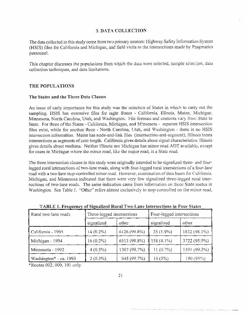
3. DATA COLLECTION
The data collected in this study come from two pnm~ sources: Highway Safety In fomlatimr System(HSIS) files for California and “Michigan, and field visits to the intersections made by Pragmaticpersonnel.
This chapter discusses the populations from which the data were selected, sample SC]ection, datacollection techniques, and da~d limitations.
THE POPULATIONS
The States and the Three Data Classes
An issue of early importance for this study was the selection of States in which to carry out thesampling. HSIS has extensive files for eight States - California, Illinois, Maine, Michigan,Minnesota, North Carolina, Utah, and Washington. File formats andcontents vary from State toState. Forthree of the States -California, Michigan, and Minnesota- separate HSIS intersectionfiles exist, while foranother three -North Carolina, Utah, and Washington there isno”HSISintersection infomation. Maine hasnode-and-link files (intersection-and-segment); [Ilinois treatsintersections asseoments ofzero length. California gives details about signal characteristics; Illinoisgives details abont mediaus. Neither Illinois nor Michigan hasminor road ADTavailablc, exceptfor cases in Michigan where the minor mad, like the major road, is a State road.
The three intersection classes in this study were originally intended to be signalized thee- and four-legged rural intersections of two-lane roads, along with four-legged roral intersections of a four-laneroadwith atwo-lane stop-controlled minor road. However, examination ofdaVd bases for California,Michigan, and Minnesota indicated that there were very few signalized three-legged rural inter-sections oftwo-lane roads. The same indication came from information on three State routes inWashington. See TabIe 1. ``Other' 'refers alnlost exclusi\elyt ostop-co]3trolledol ltllelllillorro ad,
TABLE 1. Freqrsency of Signalized Rural Tvvo-Lane Intersections in Fear States
Rural two-lane roads Three-1 egged intersections Four-1egged intersections
signalized other signalized other
California -1995 14 (0.2VO) 6126 (99.8YQ) 3j (1.9%) 1832 (98. IYo)
Michigan -1994 16 (0.270) 6513 (99.8%) 158 (4.1%) 3722 (9j.9%)
Minnesota -1992 4 (0.3%) 1307 (99.7%) 11 (0.7%) 1591 (99.3%)
Washington* -ea. 1993 2 (0.3%) 645 (99.7%) 10 (5YO) 190 (9j’)4)
*Routes O02, 009, 101 only.
21
but incIudes a few cases of flashers, and stop-controls on the major road. Of chief conce]m is not thelow percentages, but rather the low absolute numbers, which might mal<e acquisition of samples ofadequate sizes difficult. Thus, these intersections were replaced by three-legged rural intersectionswith four-lane major roads and two-Iane stop-controlled minor 1egs.
Table 1 reveals a similar, but less drastic, shortage of four-legged signalized rural intersections oftwo-lane roads. CaIifomia has relatively few of thenr, especially for such a large State. On the otherhand, Michigan appears from this table to hz, e an adequate number for sampling.
In order to gain useful variety in the analysis, California and Michigm were chosen for the modelingeffofi, with the possibility, if resources permitted, of addition of a third State later.
Constraints imposed on the populations from which the samples were chosen were as follows:
1. Thee-1egged rural intersections, major road four-lane, minor leg two-lane stop-controlled:median width less than or equal to 36 feet (11 meters) on major road, all approaches two-way, stop-controlled on minor leg only.
2. Four-1egged rural intersections, nlajor road four-lane, minor legs two-lane stop-controlled:median width less than or equal to 36 feet (11 meters) on major road, all approaches two-way, stop-controlled on minor legs only.
3. Four-1egged rural signalized intersections, major and minor roads two-lane: all approachestwo-way.
Implementing these constraints was not completely straightforward. The California (CA) andMichigan (MI) HSIS intersection files had no information on whether intersections were trurai orurban, nor on median widths, while MI’s intersection fiie had no information on number of lanes.To obtain these items, the intersections were linked with segments in the CA and MI Roadlog fileswhere such information was available.
For CA, a Roadlog variable entitled RU_IO was available to indicate whether the segment was rural,urbanized, or urban and inside a city or outside a city. For this study, we elected to use thosemarked as “rural, outside city” and did not include those that were rural, but inside or partly insidea city. The numbers for CA in Table 1 would have increased by only a small amount if other ruralcategories were added. For MI, a Roadlog variable entitled RURURB, with three rural categories(rural, rural dense small city, and rural small city boundary), was available. In the case of Mic.higsm.all three categories were allowed. Roughly 500/0of the Michigan intersections fell uncier “1-urLL~’androughly 500/0under “rat-al dense small city,” and very few fell in the third category.
An intersection in CA or MI was considered rural if a neighboring segment was rural according tothe classification above. In addition, in tbe case of Michigan, since the intersection ii Ie did notinclude a lane count, the major road was assumed to be either two-lane or four-lane, depending on
22

how the segments adjacent to the intersection were described in the Michigan Roadlog file
Pilot Studies
Pilot studies were conducted from bases in Sacramento, CA, and Lansing, MI, in March and May1997, respectively, with a view to visiting all intersections sufficiently close to the State capitals asresources permitted.
In the case of California, 115 intersections in Districts 3, 4, 10, anti the noflhcrn part of 6 (within
approximately 250 miles (402 kilometers) of Sacramento) were qual ificd fol- rnern bcl-ship in the
populations on the basis of HSIS data. In Michigan, the pilot study concentrated on signalizedintersections, and 66 such intersections were identified in Districts j, 6, 7, 8, and 9 from [hc 1+S1Sdata base.
In both States, photologs were examined for all such intersections. If the photolog indicated that theintersection was not rural (e.g., curb parking, significant urban build-up for several blocks) or thelane count was incorrect or the signalization (several flashers were found that had been listed as fullysignalized) or there was an adj scent intersection within joo feet (152.4 meters) on the major road,then the intersection was eliminated. Thereafter, site visits were tmade to most of the intersections,additional intersections were eliminated by the site visit, and data were collected at the remainingones. Even among those for which data were collected, in some cases, it was uncles]- whether theyshould be considered rural or urban. Table 2 indicates the disposition of the pilot StUdy samples.
TABLE 2. Pilot Study Intersections in California and Michigan
California Michigan
sample units - three-legged 28
sample units - four-legged 27
sample units - signalized 10 23
Y intersections 6
disqualified from pbotologs 25 13
disqualified from visits 17
too remote/isolated 6 13
Total 115 66
Table 2 reveals some difficulties that were to affect the entire study. Photologs did not match whatwas in the HSIS data base in a fair number of cases, and site visits revealed that changes not shownin the photologs had also taken place. This was particularly true of the Michigan signalized
23

intersections. The Y intersections, three-legged intersections with two legs divergitlg from the third,were included in the pilot study, but it was later decided to elimimste them from the full datacollection in part because of their relative rarity. A few intersections in botb States were excludedfrom visits on the grounds that they were too remote or isolated.
The issue of how to handle remote arrdor isolated intersection sites is a rather delicate one since itrelates to both resource consumption and sample integrity. Rural intersections can be few and farbetween. To conseme resources, it is advisable to select intersections that are in close proximity toone another and to a suitable base of operation where junior highway engineers can be recruited forfield work. With Sacramento or Lansing as a base, there were numbers of intersections each ofwhich would require an overnight trip for two people, with driving time to and from and downtimebetween morning and evening traffic counts (if the site was not disqualified). While distances inCalifornia are well-known, it is less well-knowl~ that the distance from Lansing, Michigan, to thefarthest reach of Michigan’s Upper Peninsula, 550 miles (885 kilometers), is greater than Lansing’sdistance to New York City, about 500 miles (805 kilometers). Paradoxically, the most classicalityrural intersections, ones without suburban or small town features, are iikely to be far from eacl] otherand far from suitable bases of operation and thus require disproportionate resources to \ isit. Ifintersections are close to each other, within a few miles, so that a team can visit several in the sameday, the independence of the sample may be jeopardized. If they are close to a central point, suchas a major city or the State capital, they are likely to be less rural and to be in transition.
During the pilot studies, in addition to examiruation of photo logs and field work, construction plansand aerial photographs were reviewed, and the possibility of obtaining crash reports wasinvestigated. Aerial photographs, photologs, and some (but not all) horizontal construction planswere available in the Traffic Operation Office at Caltmns headquarters in Sacramento. Morecomplete computerized vertical and horizontal plans were not available, since the computer
application that accessed them was undergoing major repair and reno~,ation, At a later dale, thissystem was running, bat some plans were found to be missing and others were difficult to locate.District Offices in California, 11 in all, also have construction plans and hard-copy crash reports, butthese offices are understaffed and the Project Team was told that retrieval would take much time.Caltrans personnel did indicate that the HSIS crash file for California would have numerousvariables from which crash details could be reconstructed. Michigan had aerial photographs formany intersections in Southern Michigan taken in the years from 1972 to 1988, and some negativesfor photos from prior years. Michigan also had a library of construction plans (maps, microfilms,and hanging files, depending on the year), although a fire in 1955 had destroyed some plans andothers were misfiled. Road segments will have as many as 50 jobs and corresponding plans. Fora minor job, the plan will not show the alignments of the road. The Project Team was told tha[, irMichigm, confidentiality laws make crash reports difficult to obtain since preliminary deletions byState employees are required. Although Michigan photologs were one cycle more recent than thoseof FHWA in McLean, Virginia, numerous discrepancies were found among the HSIS files, thephotologs, and site visit observations.
24

In both the California and Michigan pilot studies, field work was done at ail intersections. Thetypical routine was a morning site visit to hand-count traffic (on specially designed tally sheets).Thereafter, radar guns were used to determine operating speeds for samples of vehicles approachingthe intersection on each leg. These measurements were made at discreetly placed locations beforevehicles began to slow for the intersection. Speeds would be determined only for the lead car in aplatoon, and the angle between the radar path and the direction of vehicle travel was noted to permitcalculation of true travel speed. T~ically, 25 measurements would be made if the leg traffic wasadeqtlate. If the traffic was light, as many measurements as a 15- to 20-nlinute stay would permitwould be made. Measuring wheels were used to pace off sight distances. Other- intersection featuresand geomet~ were recorded, as well as signal characteristics at signalized intersections. In the lateafternoon, a second traffic count would be done. In the case of Michigan, where only sig]lalize(iintersections were visited, computertied plate counters were also used to measure m i]nor icg traffic.The plate counters were nailed to the minor road at mid-day and lefi there for 24 hours. The) wererecovered on a subsequent visit to the intersection and unwrapped. Data were downloaded fromthem and they were recharged and rewrapped for the next count. Three people were required forplacement of the plate counters since traffic had to be disrupted. For all site visits, permits wererequired from District Offices, and safety precautions, including wearing of hardhats and orangevests, and placement of cones and signs, were taken.
Pilot study data were subsequently used to prepare some small special stadies. Three kinds of speeddata were compared: posted speeds obtained by inspection along intersection legs, operating speedsmeasured by radar guns, and speeds recorded by the plate counters. The plate counters alsopermitted a determination of 24-hour truck percentages, and these could be compared with observedpeak-hour truck percentages from the manual traffic counts. To assess the “intersection-relatedness”of crashes, a review was also undertaken on the area of influence of an intersection for a few pilotstudy intersections. The results of these investigations are reported in the appendix to this report.
SAMPLE SELECTION
After both pilot studies were completed, the studies were assessed and p Ians were made for thesubsequent main data collection effofl. The chief decisions made were 10 rcstricl atten~ioo to teeintersections and omit Y inters ections,4z to measure horizontal and vertical alignments at eachintersection rather than attempt to extract this information from plans or photos, to discontinue theminor leg plate counts, and to follow an informal sample selection plan.
42A three-legged intersection is a T intersection (or tee) when “two of the three intersec-tion legs form a through road and the angle of intersection is not acute”; it is a Y intersection (orwye) when “all three intersection legs have a through character or tile intersection angle with thethird intersection leg is small.” These definitions are taken from p. 836 of A Policy at? C;eo/7tet}-icDesign of Highways anti Intersections (also known as the “Green Book’), American Association ofState Highway and Transportation Officials, Washington, D.C., 1994.
25

Three-legged intersections for the main data collection efi~ort were restricted to T irrtcrsectionsbecause of the relative scarcity of Y intersections and in the interest of sample homogeneity. Samplehomogeneity contributes to successful modeling by removing variahlcs that \vi II not be modeled.However, such homogeneity can only be achieved to a limited extent. Too many restrictions (e.g.,requiting that all intersections have lighting, that they all have medians of a certain type, that theyhave ADT in a certain narrow range, etc. ) can be counterproductive. There may he Loo fewintersections meeting all the constmints to be useful for modeling, and data collection from all ofthem to maximize sample size may be too expensitc if they are geographically dispersed. Thedistinction between T and Y intersections is of recognized importance, T intersections are fa~orcdby intersection designers, and restricting the sample to T intersections was judged to pose noproblem.
Collection of alignment data during the field work and discontinuation of minor leg plate corurtswere undertaken for reasons of economy.
In both Michigan and California, the availability and accessibility of plans showing recordedalignments were in doubt. Plans and photos were sought for sub-samples of the pilot study samplesin both States, and for roughiy 30°/0of the intersections in the sub-samples, no information coLdd befound, Since morning and afiemoon traffic counts were to bt~done at each intersection, acquisitionof alignment data at midday did not seem to be unduly burdensome for field workers. Atintersections visited in the pilot studies, alignment data had not been collected, but I-cvisits duringother field work could be done without hardship.
With respect to the plate counters, the pilot study revtidied that they provided good data, but that theywere resource-intensive and that the data were not essential to the overall effoLt, The p Ia.tecountersare HISTAR units that detect changes in the magnetic field above the roadway. The associated.computer data are generated and printed with NU-METRICS software. Information availableincludes: counts of incoming vehicles by type, counts of occupants per vehicle, vehicle speeds.,weather conditions (temperature and precipitation), and gaps between vehicle arrival times. During;the Michigan pilot study, the weather variables did not seem reiiable, and the counters did not work:properly on occasion. At two intersections, they were placed on nraj or roads for whicil .4DT was
available. The count at one of these roads was 4,400 vehicles per day versus 6,400 vehicles per dayaccording to HSIS files. The difference is that the plate count data is for one day in 1997 and theHSIS data is a State estimate for 1993-1995. The plate counters do not determine turningmovements, and manual counts still Ilave to be done at each intersection to obtain these. The platecounts, as already noted, require two visits spaced 24 hours :ipart with adequate personnel to ensuresafety during placement and removal. Thus, to conserve resources, they were omitted in the maindata collection effort. For Michigan intersections where minor road ADT was not available, majorroad ADT PILLS 1997 peak-hour traffic counts, in particular mtios of traffic by movement, were usedto estimate minor mad ADT. This method, while making use of 1997 data to estimate minor roa(iADT for earlier years, is arguabIy more reliable than using an absolute 1997 count.
26

Both pilot studies revealed that field work at rural intersections is time-consuming. Ruralintersections suitable for the study, especially signalized ones, tended to be few and far between, asnoted earlier. In some cases, overnight lodgings were required both before and after in order forProject Team members to get to a site at an adequately early hour and remain there unti 1 an.adequately late hour. During the Michigan pilot study, a number of intersections thought to be inthe population on the basis of HSIS files and Michigan photo logs were found to be unqualified ata site visit, primarily because they were not at all rural.
Au informal sampling plm, as follows, was developed. Complete lists of intersections whose HSISrecords satisfied the constraints had been developed. All intersections within approximately a 3- to4-hour drive from Sacramento or Los Angeles or Lansing were automatically included in the sample,together with a few other selected intersections at farther distances. Photo logs we]-e reviewed forall of these, some were disqualified as a result, and with the exception of those tha[ bad been in thepilot study and a few especially remote ones in California, all of the remaining ones were pre-visitedprior to the field work. The purpose of the pre-visit was to ascertain whether each intersection was.in fact, qualified — no legs or medians closed, no offsets, no additional lanes or legs, number oflanes unchanging out to +800 feet (243.8 meters), no urbanization, wi /h signal ization or sign age asadvertised. In addition, a large number of intersections were eliminated because they were too closeto other intersections of the same type and were likely to have strongly correlated data values. Thiswas especially true for the three-legged and four-legged non-signalized intersections. In ‘botb States,such intersections tended to be grouped on a relatively small number of highways and tende(i [o bcplaced along these highways in close sequence.
Pre-visits by senior Project Team members were found to be very useful since field workers would.not spend unnecessary time at unqualified intersections and tbe senicr members of the team couldmake experienced judgments about the appropriateness of intersections.
The final samples, including pilot study obsemations, are shown in Table 3.
TABLE 3. Samples as Proportions of Nominal F’opulatians
CA MI ToPdl
3-legged 60/302 (19.9VO) 24193 (25.8VO) 84/395 (21 .3YO)
4-legged 54/150 (36%) 18149 (36.7Ya) 721199 (36.2 V”)t
Signalized 18127 (66.77,) 31/100 CIIYO) 49/127 (38.6%)
The first number in Table 3 is the sample size and the second is the nominal population size in theState. These numbers are adjusted from Table 1 by elimination of duplicate observations aniphotolog reviews, but the denominators include numerous dependent intersections and, especiallyin the Michigan signalized case, intersections that are no longer rural. The denominators alsc
27

include remote intersections that were not visited for lack of resources. It shouId be kept ill lnindthat some of these would have been disqualified if they had been visited.
The informal sample selection method raises the issue of represenrativ:ness. It should be noted thatcrash data were not consulted in selecting the samples, but that there was some tendency to f~lvorlager mT intersections or ones with more irregular alignment when, for example, Only One 01’two
nearby intersections could be chosen because of dependence. In addii:ion, many, but not all, of the
most remote intersections in both Statci were omitted from the samples.
DATA COLLECTED
The data collected in this study and the sources are sl?own in Tab Ic 4.
Highway Safety Information System (HSIS) Data
Average Daily Traffic (ADT) data and crash data were extracted from HSIS files.
~Tdatawere extracted from HSISIntersection and Roadlog files. ForCalifornia,r ndjorandminorroad ADT were available in HSIS intersection files for the years 1993, 1994, and 1995. ForMichigan, ADT data were available in HSIS Roadlog files for segments of State roads, although1993data were Llnavailable andhadto beinte~olated from 1992 data.
HSIScrash vanablesfor 1993, 1994, and1995 were consulted. These illclLlde Accident Locationvariables, Accident Number, Accident Severity, Accident Type, N’umber of Vehicles, VehicleMotion Prior to Accident (MISCACTl). Allvariables, buttFJe last, areillthe HSISAccidellt lile forthe State. The Iastisin the HSIS Vehicle file.
Traffic-Count Variables
For all intersections in Ole study, field counts were done c,n traffic during nlOrlling and eveninghours. Duetolimited resoL]rces, lhecounts were llotdonea .tafixed" iime,bLlt\veret ypicallyd oneinthemoming forabout45 minutes between 7:00 a.m. and 9:30 a.m. aod in the aftemoonbetw,een3:30 p.m. and6:O0 p.m. Thecounts were done onnon-holiday weel<days.
In a few cases in California, no traffic was seen emanating from the minor road during the hours ofvisitation. Th~shappened at Wothree-legged intersections and at two four-legged intersections, allof them in California on Route 395. The first twointersectio:ns hadincoming traffic, butthelasttw()hadnOtraffic, inconling oroutgoing. These intersections zreinhigh-altit~lder egionsnearMon()
Lake and Independence, the counts were made in the fall of 1997, and traffic may have been reducedfor seasonal reasons.
28


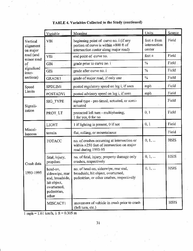

During the counts, the number of passenger vehicles and the :number of trucics entering and leavingthe intersection were recorded, along with the incoming and outgoing legs. The beginning andending times of the counts were also recorded. A typical dumtion was 45 minutes. When the datawere processed later at Pragmatic, Inc., aIl counts were converted to hourly counts. Intersectionlegs were identified by leg numbers, in the clockwise order 1, 3, 2, 4 shown in l;igure 1. Legsnumbered 1 and 2 are on the major mad; ~rom leg 1 to leg 2 is the increasing milepost direction.Legs 3 andor 4 are on the minor road, with leg 3 to the Iefi of the major mad’s increasing direction.For traffic going from leg number i to leg number j, the morning counts were M_.PCij aad M_TRijin vehicles per hour, while the evening counts were E_”pCij and E_TRij. The di stinct iOn betweetlpassenger vehicles and commercial vehicles/trucks was based on the number of tires. A commercialvehicle was taken to be any vehicle with more than four tires, and included cars with trailers. Thisalmost always meant a vehicle with more than two axles.
Major Road
Leg 2
~. Increasingmilepostdirection
ANGLE1 ,1i$TGL B2
Leg 3 Lecy 4
Leg 1
Major Road
FIGURE 1. Intersection Diagram Showing Leg Numbers
Roadside Variables
During the field work, the roadside variables Number of Driveways and Roadside Hazard Ratin\;(HAZWT) were col[ected by inspection.
The number of driveways within 250 feet (76 meters) of the intersecl:ion center was counted aloll{~the major road. Residential and commercial driveways were counted separately. A gas station withtwo entranceways would be counted as having two commercial driveways. For signalize(iintersections, the number of driveways was also counted on the minor road out to 250 feet (76meters).
32

HAZRAT is a vwiable devised by Zegeer et al. (1987)”3 that !s an amaigam of sideslope, clear zone,and distance to nearest hard object. It takes who[e number values from 1 to 7, with 7 being the mosthazardous. Field workers were provided with images of typical roadsi(ies with different ratings, andat site visits, they made estimates of the average rating of the major road ~vithin 250 feet (76 meters)of the intersection center.
Channelization and Intersection Geometry
At each intersection, field workers recorded left- and right-tu.ming lanes on all approaches, medianwidths and characteristics, and intersection angles. At a three-legged intersection, the numbet- of left-tum lanes on the major mad, or right-turn lanes, is always CIor 1, and likewise on the minor road.At a four-legged intersection, signalized or not, the number of lefi-turn lanes on each road, or right-tum lanes, is O, 1, or 2. The measured intersection angles, AhTGLE1 and A.NGLE2, are bet~veen legs2 and 3 and between legs 2 and 4, respectively. See Figure 1. In California, intersections aresquared up by policy, i.e., although the basic angle between the major and mirror roads may besubstantially different from 90 degrees, the minor road wi 11curve shaiTly wit 11in a feiv car lengthsof the intersection to create a right angle. Field tvorkers were itlstructe~j 10 ]rccord the large-scaleangle of the approach when very sharp curves of this type were present.
Sight Distances
Sight distances \vere estimated longitudinally on the major road and left and right on each minor leg.At three-legged intersections, the longitudinal sight distance was only measured in one direction,,e.g., if the third leg was leg 3 in Figure 1, then the sight distance from leg 1 to leg 2 was measured.,but not from leg 2 to leg 1. Like\vise, at signalized intersections, Iefi sight distances were notmeasured. For the signalized intersections, longitudinal and left sight distances \vere estimated onall legs. When a protected lefi turn exists from leg 1 to leg 3,,one may argue that longitudinal sighl:distance from leg 1 to leg 2 is unimportant.
The Green Book (1994, p. 702) recommends that left and right intersection sight distances fi-om theminor road be measured at 6 meters (20 feet] from the edge of the traveled way. At manyintersections, this yields very little sight distance, and only a foolhardy driver would decide to enterthe intersection from this location. An alternative standard is 3 meters (10 feet) from the edge of thetraveled way, approxim~tely the location of a seated driver prior to [entering the intersection. Thelatter standard has apparently been adopted by many States, and is the one that was used ir]measurements here. For longitudinal sight distance (along the rnaj or road from one lane to the
opposing lane), measurements were made from the edge of tbe traveled ~vayof the minor road i11the
leftmost incoming lane of the major road. The driver’s eye \vas assumed to be at a height of 1070
millimeters (3,5 feet) and the object viewed was assumed to have a height of 1300 mil 1imeters (4.2!~
43C,V, ze~eer, j. Hummer, D. Reinfuhrt, L. Herf, and W. Hunter, safety Co~t-
Effectiveness of Increilletltal Changes in Cross-Section Design — Information Guide, Report No,FHWA-RD-87-094, Federal Highway Administration, Washington, D. C., 1987.
33

feet). See the Green Book, pp. 136-7
Sight distances, if they were sufficiently short, were paced off with a measuring wheel to record thedistance. If they were many hundreds of feet long, they were estimated with a range finder. Thelatter is an optical device with two light paths from the distant object to the eyepiece. Then a dialis turned until the two images of the object merge, and a distance can be read from the dial.
Horizontal Alignment
Horizontal curves were recorded for the major mad and, in the case of signalized interst~ctions, forthe minor road. A segment from 800 feet (244 meters) before the intersection to 800 feet after theintersection was determined, and any horizontal curve thdt over[appcd this segment was inc Iuded.For each such horizontal curve, the beginning and end points were noted, along with the directionofcurvat~lre and the degree of curve, Measuring wheels and chalk were used to determine beginningpoints and endpoints. Degree of curve was measured by marking off a straight line dis~ance,t~ically 100 feet (30.5 meters), between two points at the edge of the (:raveled way, and calculatingthe perpendicular distdace at the midpoint to the edge of the traveled way. The degree of curve, indegrees per 100 feet (30.5 meters), is then calculated from the formula:
where L is the length of the straight iine in feet and H is tht;pe~endicular distance in feet, (The
metric equivalent is DEGH,,, = DEG/O.305 in degrees per 100 meters.) No adjustment was made forthe roadway width, Eveo on a four-lane road, au adjustment that rep] aces the edge of the traveledway by the centerline of the road would typically change the value by no more than a few percent.
Vertical Alignment
As with horizontal curves, vertical curves were recorded that overlapped a segment out to + 800 feet(244 meters) from the intersection center along the major road and:, for signalized intersections,along the minor road. Beginning points and endpoints of each vertical curve were deternlined with.measuring wheels and chalk. Then, incoming and outgoing grades were estimated at the beginning,and end of each curve. Grades were considered positive if they were uphill in the direction horn leS1 to leg 2, the increasing direction of the major road, or from leg 3 to leg 4 along the minor road,For any intersection that had no vertical curves, a unique grade, GMDE1, was reported.
Grades were measured in one of two ways. An optical level and a measuring rod were sometimesused, A distance of 25 feet (7.6 meters) or so would be pacecl off along the edge of the traveled way.A marked height at that distance wouid be compared with the corresponding height on a measurin~;rod determined by sighting the optical level horizontally. The diffel-ence in height divided by th,~
34

horizontal distance yields the slope. An alternative method ‘was to pk~ce a 4-foot (1.2-meter) levelalong the roadway (or along a flat board on the roadway) and record the slope directly from adisplay.
Other Variables
Posted advisory and regulatory speeds were recorded for each leg whe:l seen within a few thousandfeet, existence of lighting at the intersection was noted, and a qualit~,iive measure of terroul (Lui,rolling, or mountainous) was also noted. At signalized inters(~ctions, it was noted whether the signal
appeared to be pre-timed, actuated, or semi-actuated. Protected left turns on the major road were
also noted, but no record was made of which pairs of legs had such protection. A reasonableassumption is that the left-turn movement from the major road leg with the highest volume, eitherleg 1 to leg 3 or leg 2 to leg 4, had such protection when PROT_LT equals 1 and no left turns wereprotected when PROT_LT equals O
DATA LIMITATIONS
HSIS Data
The HSIS variables are ADT and crash data for the years 1993, 1994, and 1995
California ADT data are determined systematically and regularly on State roads through 40Cpermanent continuous operation count stations and another 1,700 permanent stations that are useconce every 3 years. Intersection major road ADT is based on the segment ADT. Minor road ADTis generally estimated rather than counted, is done by the Districts, and is thought to be older ancof lesser quality. Michigan has about 120 pemanent count stations, nOt al1 on State roads, andattempts to do counts on each State road once every 3 years. It does not have ADT for minor roadsunless they are State roads.
Crash data for both States are subject to the limitations noted in the study of Hakkert and Hauer(1988). Many Michigdo property damage only crashes, and some injury crashes, are reported by thedriver without an officer at the scene. Not only are there issues of underreporting and classificationfor both States, but there is also the question of crash location. Some iMichigan observers think thdt
crash locations are often incorrect, and mention examples where a crash was attributed not j ust tothe wrong milepost, but to the wrong intersection.
Field Data
The traffic data collected in the field during this study have obvious linlitations. They were collectedon a single weekday in a particular season of the year and during a short time period in nominal peakmorning and evening hours. Field workers reported that in different locations, the traffic vOlumes
might be especially high early or late in the morning Or evening, depending On such cactors as the
35

~re~ence Of a manufacturing plant versus a shopping center nearby. The tme definition ofpe~ hour
varies from location to location, while this study had to follow visitation timetables based onavailable resources. In California, some rural intersections had relatively low traffic, reflecting likelyseasonal variations at resorts and camping areas such as Lake Tahoe. The site visits were conductedin late fall and early spring at some of these locations. No attempt was made to adjust the data totake into account such variability. Yet another limitation is that these data were collected in 1997for use in modeling 1993-1995 events.
Variables such as HAZWT, number of driveways, chan~elizatior), angle, speed iinlitst sightdistances, and horizontal and vertical alignments were also measured in 1997 and are presumed tobe valid for the earlier time period. These items, however, tend to be much more stable than trafficmovements, and temporal variation is not thought to be a significant source of error.
HAZWT is a subjective rating of roadside hazards. The measure is supposed to average the hazardsalongside the major road within +250 feet (76 meters) of the intersection. Typically, twoexperienced observers will agree on a value or differ by 1, e.g., one observer may assign a 3 and theother a 2.
Sight distances, as noted, were measured with a measuring wl~eel or a range finder. Because of thelimitations of the range finder and some subjectivity about when an object becomes vis~ble (seeingsomething versus recognizing what it is), sight distances are likely to be accurate to within roughly10OA. For the purposes of this study, sight distances in excess of 1800 feet (550 meters) or morewere not distinguished, and any sight distance thought to be in excess of 2000 feet (610 meters) wasgenerally marked as 2000 feet. A sight distance of 1600 fset (488 meters) would be noticeablysmaller, and absolute accuracy would improve as sight distances decrease.
Horizontal and vertical cumes present unique difficulties. For many rural roads, the line of ahighway is quite irregular when examined on a small scale. Potholes, bumps, and other smallirregularities due to the lay of the land or due to wear caused by traffic and weather are often present.Field workers were asked to idealize roadways by smootbi.ng road !.ines out to scales of severalvehicle lengths. Decisions about where a curve begins and ends are thus to some extent arbitrary,particularly for curves of large radius or small grade. “Beginning points and endpoints as judged bytwo different obsewers might differ by as much as 20 feet (6 meters), while degree of curve might
vw by 5°/0or more. Michig~ was relatively flat, with many grades lI~SSthan 10/O.ver~ical gradesof less than 1‘A were probably measured to no greater accuracy than 4:0.250/., so that a grade listedas 0.50/0 might be 0.2j0A or 0.75°4. A much larger grade, say 5°/0, would be accurate to within*0.50A. Differences in successive grades accompanying a vertical curve would have about the sameaccuracy since the observers would be sensitive to the chan,ge of grade.
perhaps tbe greatest limitation of the data is that they do not reflect the special circumstances Ofeactl
intersection. men individuals are classified by such conventional (and imperfect) measures as age,height, weight, sex, IQ, race, etc., sometimes the most important and most relevant points aremissed. Site visits reveal that the intersections in this study are quite diverse, with very individual
36

personalities. significant items fhat would not appear in a cia!a base are quite common, e.g., a
nearby amusement park, beach turn-offs along Lake Huron, canyon roads off of Pacific coastalhighways, sideroads into California deserts, resort areas such as Lake Tahoe and Squaw Valley,small tows where a two-lane road flares out to four lanes for a few thousand feet or where a two-lane road abruptly arrives at a single signalized intersection, or rural intersections along heavily
trafficked commuter highways connecting big cities to rural homesites.
Signalized rural intersections, in particular, are in transition. ‘rhe signal is often in place because ofincreasing local development and increased minor road traffic. With increasing traffic come morebusinesses and residences, and soon a very roral area becomes a small town and a small townbecomes a city.
Analysis and modeling are bound to be inexact because the population under study is a movingtaget, and qualitative changes can overtake the quantitative ones, bringing unforeseen variables into
prominence.
37

4. ANALYSIS
The analysis consists of developing a variety of new vtiables derived from the variables collected,determining the statistics for new and old variables singly and jointly, determining correlationsbetween variables (especially between crash counts and other variables), and studying the chiefrelationships found.
Of particular interest is the relationship between crash counts and traffi{:. Without question, averagedaily traffic (~T) on all approaches is a significant (and usually the most significant) predictor ofcrashes. Not only does greater traffic imply greater numbers of crash-prone dtivers, even with thepercentage of crash-prone drivers assumed to be independent of traffic or increasing with traffic, hutfor multiple-vehicle crashes at intersections, an adequate amcunt of tra.ftic is a necessary conditionfor a crash.
Successive sections of this chapter treat new variables, univariate stati sties, b ivariate stati sties andcorrelations, and the relationship between crash counts and traffic.
NEW VARIABLES
The chief classes of variables in this study are: crash va]-iables, traffic variables, intersectiongeometric variables, roadside variables, alignment variables, and sigh’: distances. The intersectiongeometric variables concern medians, channelizatioll, and lntersectiOn angle. Alignment variablesand sight distance variables, which pertain to the roadway as far out as 800 feet (244 meters) toseveral thousand feet from the intersection center, are treate(i separately.
Crash Variables
The chief crash variable is TOTACC. This is the total number of crashes occurring at theintersection in the years 1993, 1994, and 1995. Any crash occurring at the intersection or within 250feet (76 meters) of the intersection center along the major road is included in this number. Crashesoccurring along the minor road near the intersection are recorded as being at the intersection (ifwithin 100 feet (30. 5 meters) of the intersection center in Michigan, if within 250 feet (76 meters)in California). One exception to this is when the minor road is a State road (the major road is alwaysa State road). This happens for some signalized intersections. In suck cases, Accident IiIes for the
minor road were also consulted and all crashes within 250 feet (76 meters) of the intersection centeralong the minor State road were included.
A second crash variable is TOTACCI. For this variable, criteria proposed by Bellomo-lMcGee, Inc.(BMI) were used to restrict the crashes to ones considered intersection-related Michigan’s HSISAccident file has a variable called Highway Area Type that indicates whether a crash occurred in thevicinity of an intersection. This perhaps could have been used to es~ablisb intersection-relatedness.However, California has no similar variable. Indeed, an important modeling issue IS to establish
39

criteria for intersection-related crashes that are uniform from State to State. A set of criteria withthis aim were prepared by Warren Hughes and A.J. Nedzesky of BMI, with the assistance of ForrestCouncil, and were submitted to FHWA in a memo dated March 26, 19’98. The BMI criteria are thefollowing: (1) crashes must occur within 250 feet (76 meters) of the intersection center aod (2) they
must be (a) vehicle-pedestrian crashes; (b) crashes in which one vehicle involved in the crash ISmaking a left turn, right turn, or U-turn prior to the crash; or (c) multiple-vehicle crashes in whichthe accident type is either sideswipe, rear end, or broadsidelangl e.
Applying these criteria in California and Michigan was not cc,mpletely straightfomard. M inor roadcrashes could sometimes only be obtained out to a lesser distance, as noted above, beCaLISc of the
recording methods of the States. The California data base is silent on whether crashes, includingturning crashes, may or may not involve driveways, while Michigm has separate categories for sOnlecrashes involving driveways (e.g., “angle driveway”). For accident t,ype, California uses the term“broadside,” while Michigan uses the terms “angle straight” and “angle turn.” California does notdistinguish between “sideswipe same” and “sideswipe opposite,” whereas Michigan does. Theprecise criteria used in the two States, apart from location as specified in TOTACC, were:
or
or
or
or
or
CALIFORNIA
Some vehicle in the crash had MISCACT1 (Motion preceding collision) equal tc “makingright turn, “ “making left turn, ”or “making U turn”;
ACCTYPE (Type of collision) was “Auto-pedestrian”;
VEH_INVOL (Motor vehicles involved with) was “Pedestrian”;
VEH_INOL was “Other motor vehicle” or “Motor vehil;le on other roadway,” and ACCTYPEwas “Sideswipe” or “Rear end’ or “Broadside.”
MICHIGAN
ANALYS (Accident analysis) was “Motor vehiclelmot(jr vehicle,” and ACCTYpE (Accidenttype) was “Head-on” or “Sideswipe opposite,” and MISCACT 1 (Driver intent) for some vehiclein the crash was “Make right turn, “ “Make left turn,” or “Make U turn”;
ANALYS was “Auto-pedestrian”;
ANALYS was “Motor vehicle/motor vehicle,” and ACCTYPE was “Angle straight,”“Rear end,” “Angle turn,” “Sideswipe same,” “Rear end lefi turn,” “Rear ‘nd ‘ight ‘L!m,”“Head-on lefi turn,”” Dual ieft turn,” or “Dual right turn.”
From these comparisons, it is evident that the problem of uniformity among States also arises whel:.multiple data fields are used to ascertain whether an crash i.s intersection-related. Tbe data fields
40

and associated definitions do not always match up precisely
Yet another problem is that the BMI criteria were developed for use with two-lane rural roads. The
present study, in part, concerns four-lane rural roads and it is not clear that the same criteria shouldbe used for them. Observers have also raised the issue of whether different criteria should be usedfor signalized versus non-signalized intersections of two-lane rural roads.
Four other crash variables were developed for this study. Their definitions are given below:
,NJACC = Aall accidents with fatalities, injuries, or possible injuries counted in TOTACC
INJACCI = All accidents with fatalities, injuries, or possible injuries counted in TOTACC
TOTACCS = All single -vehicle accidents counted in TOTA CC
TO TACCM = All multiple -vehicle acciden(s counted in TOTA CC
The first two variables, INJACC and INJACCI, exclude crashes in which only propelly damageoccurred, but include all others. In California, one of the severitY categories is “COnlPlaint of Pain”In the time period 1993 through 1995, the reporting threshold for property damage only crashes was
S400 in Michigan and $500 in California. The last two variables, TOTACCS and TOT.4CCM, weredetermined for the signalized intersections only, and were used in some of the rnodeiing to relatecrashes to traffic flows by leg.
ADT Variables
Two average daily traffic variables were used in this study - ,4DT1 and ADT2. ADT1 is estimatedaverage daily two-way traffic on the major road measured in vehicles pel- day (vpd) in the vicinityof the intersection for the 3 years 1993, 1994, and 1995. ADT2 is the estimated average daily two-way traffic for the minor road in this period.
For California, ADT1 and ADT2 were obtained by taking annual figures provided in the HSISintersection files, samlning them, and dividing by three.
For Michigan, ADT data were not available in the HSIS intersection file. However, ADT data wereavailable in the HSIS Roadlog file for State roads in the yearn 1992, 1994, and 1995. The values o:ADT for these years were interpolated to obtain a value for the year 1993, and the values for 1993,1994, and 1995 were averaged. These estimated ADT values were for segments of roads. Then,ADT on segments of the major road adjacent to intersections in the study were averaged to yieldADT 1. In some cases (about 20Y. of the Michigan intersections), the minor road was also a Statt;road, and ADT2 could be obtained in the same way. In all other cases, ADT2 was estimated on th(;basis of morning and evening traffic counts done by Prag,matics, I:nc. (see below). An averagf:morning-hour traffic count (incoming plus outgoing) was tletermined for each leg, converted into
41

a haction of all incoming and outgoing traffic; the same wa, done for evening traffic, and the twofractions were averaged. Then this fraction was applied to the known estimated ADT on the twolegs of the major road to obtain an estimated ADT for each minor leg. ADT2 was this value if therewas only one minor leg, and it was the average of the values for the NO minor legs otherwise. Thismethod has two evident defects: it only represents peak-hour .ADT, and a sample of such at that, andit was done in the year 1997 rather than the study years. Nonetheless, it probably has the correctorder of magnitude and may well be as reliable as other minor road ADT estimates in the HSIS h les.
In the case of the signaltied intersections, the decision about which of two two-lane roads at a four-Iegged intersection is major and which is minor was based on. ADT. The one with the higher ADTis defined to be the major road, and the other the minor mad. In general, the major road is the Stateroad, but in Michigan, ‘sometimes both roads are State roads and thus the ADT criterion is used todeclare one of them to be the major road. There are three cases, two in Michigan and one in
California, where the State road has a lower ADT than the c~therroad, a county or local road. Inthese three cases, the other road is tal<en to be the major mad, its ADT is ADT 1, and its legs aretaken to be legs 1 and 2.
Variables Derived From Traffic Counts
Traffic count data were converted into hourly form so that for each ordered pair of approaches (i,j),an estimated number of vehicles per hour was given traveling :&omleg i to leg j. This was calculatedfor passenger vehicles and trucks separately and for a morning and evening hour separately.
M_Pcq =RA WMPCq
M_HR
M_TR~ =RA WMTRq
M_HR
E_Pc~ =RA WEPCq
E_HR
E_TRv =RA WETRq
E HR—
A rather large variety of variables can be derived from such quanti!:ies. For the present study,selected variables shown below were developed.
Commercial or truck percentage was measured by three variables, Ahfl’7”l”RUCK, PM Y”TRUCK,and PKO/OTRUCK, representing the morning, evening, and combined morning and eveningpercentages of truck traffic passing through the intersection. These are defined as follows:
42

AMYoTRUCK =L.l, ,.,,.,,,,, ~-TRij
E
x 100~,,PO,,~<,J1(M_TRij + M_pCT)
~.,, p.,,,, (i,,(~-TRV‘E-TRU)
‘K%TRUCK=E“),p..,(i,j, ‘“-TRV + ‘-PCV + ‘-TRV + ‘-pCo)x 100
The sums are over all ordered pairs of legs (i,j), i #j. Notice that PKPATRUCK is not necessarilythe average of the other two variables. It is rather a weightec! combination of the two, weighted bythe fractions of the overall traffic in morning and evening, respectively.
Turning percentages were calculated along tbe major road, the minor road, and combined bymethods similar to the above. Define the auxiliary variables Mij and Eij by:
summing passenger and commercial vehicle flows to get tctal vebicie flOWS. Then, the variables
PK%TURN, PK%LEFT, PK%THRU1, PKYoLEFTl, PK%THRU2, PKV.LEFT2 are given by:
PK%LEFT = z ~ —(rJ) (1,3)(41).(2,4), .? (34)M~ + Eq
x 100~,, ,“,,$ ~,,,, (Mv + Ey)
43
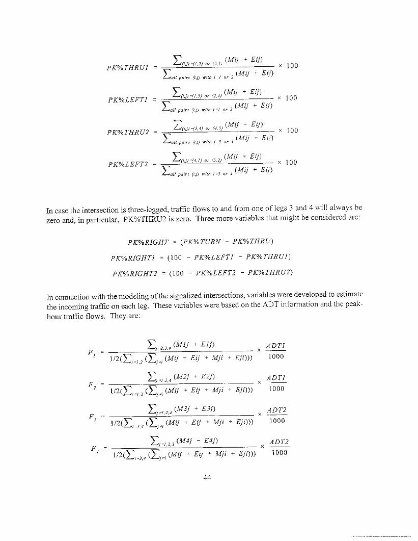
PKYo THRUI =
PKYoLEFTI =
PK%THRU2 =
PKYOLEFT2 =
In case the intersection is thee-legged, traffic flows to and from one of legs 3 and 4 will always bezero and, in particular, PKO/0THRU2 is zero. Three more v:?riables tllatnlight beconti.dered are:
PKYoRIGHT = (PKYo TURN PI<YoTHRU)
PKYo RIGHTI = (100 - PK%LEFT1 - PKY. T15RUI)
PK%RIGHT2 = (loo - PKYOLEFT2 - PK%THRU2)
In cmmection with the modeling of the signalized intersections, variables were developed to estimatethe incoming traffic on each leg. These variables were based on the A13T information and the peak-hour traffic flows. They are:
z,.,,,,,,(~lj + Elj) ADT1F, = _x——
I IZ(~i=,,2 (~j~i (Mq + Eq + ~ji + Eii))) ‘[000
z,.,,,,,, (M2j + E2j) AD TIF2 = _x—
112(X,=,2 (Xi,i (MV + E~ + Mji + ~ji))) 1000
z,.,,,,, (M3j + E3j) ADT2F, = _x.—
112(ZI=3,4 (Xj.i (MU + Eij + Mji + Eji))) 1000
Ej,,,,, (~4] + E4J) ADT2F4 = —x.—
1/2(xi .3,, (xi+, (Mu + EV + Mji + ,Eji))) 1000
44

where the units are thousands of vehicles per day and Fi is the estimated nunrbcr of thousands ofvehicles per day entering the intersection along leg nLlmber i (c f Figl.tre 1). Tb[-ee other variablesderived from the Fi’s were also considered:
PRODFADJ = F,Fd + FdF2 + F2F3 + F3F,
PRODFOPP = F1F2 + FjFd
SUIWF = F] + Fz +F3 + F,
The first variable PRODFADJ is a variable representing the interactiol~ of adjacent legs, the secondPRODFOPP does the same for opposite legs, and the third SUMF is the sum of all the flows.
Intersection Angle Variables
h angle variable DEV, representing the average deviation from 900, is defined by:
/a8gleJ - 90/ if in/ersectiOn is tkr.e -legged with third leg lefi (leg 3)
DEV = 1ang”2- 901 if intersection is three -legged with rhird leg right (ieg 4)
~anglel - 90\+langle2 - 901if Intersection is fouf –legged
2
Another angle variable considered in this study, suggested by E. Hau.er, is HAU:
angle2 - 90 if the third leg is to the right (leg 4)at a three –legged intersection
90 - anglel if the third leg is tO the left (leg 3)HAU = at a three –legged intersection
angle2 - anglelat a four–legged inti?rsection
2
The variable HAU is a signed variable. See Figures 2 and 3. For a three-legged intersection withthe angle to the right of the increasing direction, HAU is positive when the angle is larger than 900,as in 2(a), and HAU is negative when the angle is smaller thm 900, as in 2(b). If the angle is to thf:
left of the increasing direction (see Figure 3), 180” minus the angle becomes the new angle andHAU is defined as ((180 - angle) 90) = (90 - angle), as above. For a four-legged intersection, asin 2(c), it is tbe average of the two three-legged values (and thus 900 cancels out). Figure ‘$illustrates the calculation of HAU in a variety of cases. Kulrnala (1995) proposes that turns from the
45
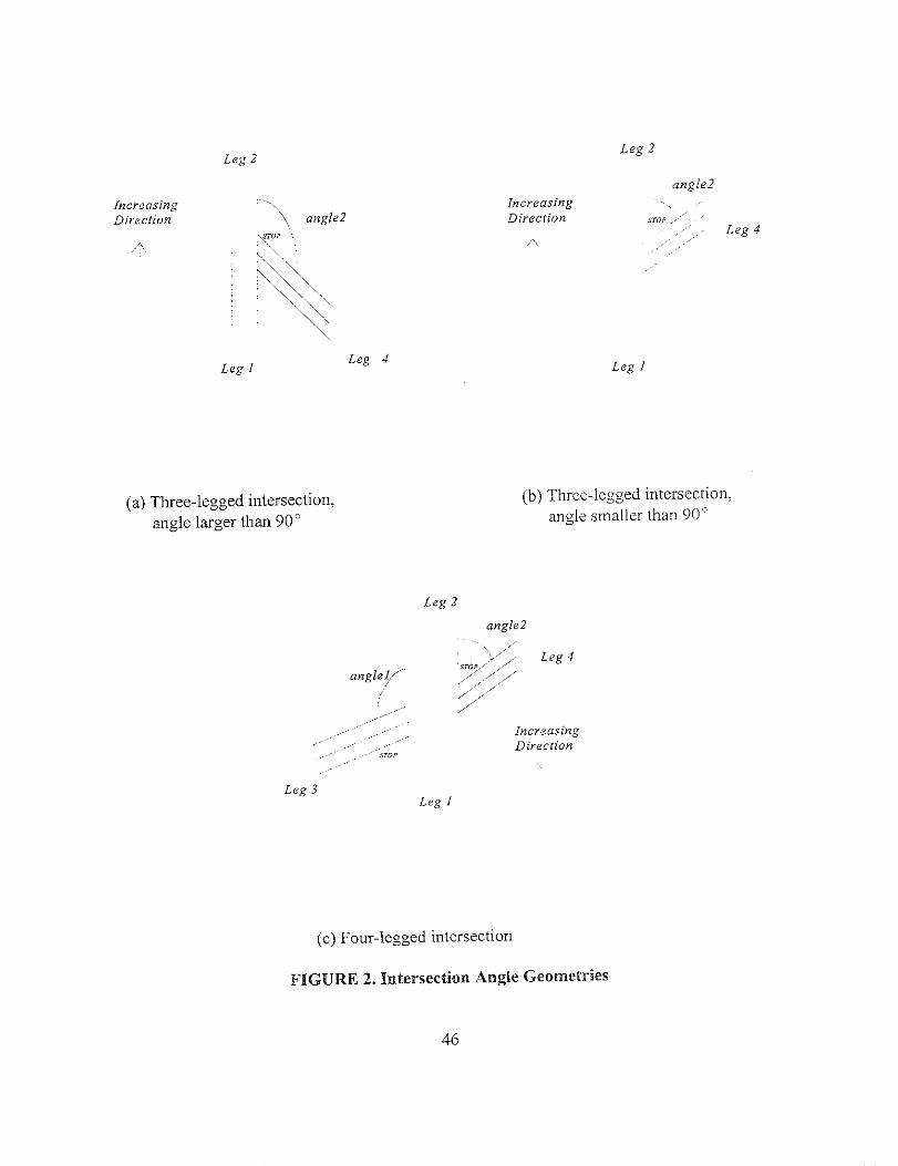
Leg 2Leg 2
IncreasingDire cti”n ““”\, aHgle2
.<7”F.4 \\.
\
& \.\
<
Leg 1Leg 4
(a) Three-legged intersection,angle larger than 900
(b) Three-legged intersection,angle snlaller than 90°
Leg 2
angle2
,,..\.y Leg 4
,,0,,, ,/’,,/ ,/ ,,,/
,’ ‘,”,/”
I,vcreasi.g
Direcrion
(c) Four-1egged intersection
FIGU= 2. Intersection Angle Geometries
46

For Three-Legged l.tersections:
Mi”orrozd to ciQht Of m.i. rv.. d 1. dice. ti. n of incceaslng mile~. st$:
t T
L135°
k
90,.,.
\,
HAU = ..01.2 -90 HAU = a“Q1e2 -90
=135-90 =90-90
= 45 =0
Minor road to left of major road in direct!. ” of increasing mileposts:
HAU = 90 -a”glel HAU = 90 -anglel
=90-80 =90-90
=10 =0
For Fo. r-Legged Intersections:
(minor road not straiQht)
HAU = (a”gle2 -anglel )12 HAU = [Snglez -a” Qlel )/2=(110-80)/2 =(90.901/2=55 =0
P60,
HAU = a“Qle2 -90
=60-90
= .30
115°
4
,,’
IHAU =90. angle<
=90-t?5
= -25
4
HAU = (angle2 -an Qle1112
= (60 120)/2
= .30
FIGURE 3. Examples of Calculation of the Angle Variable HAU
47

far lane of the major road maybe less crash prone in situation 2(a) thdn in situation 2(b), so that.positive values of HAU correspond to fewer crashes.
Sight Distances
To represent sight distances for the modeling, reciprocals were chosen. Large values of thereciprocals corresponded to poor sight distances, and small ones corresponded to lengthy sighl.distmces, and thus crashes might be expected to increase with increasing values of the reciprocals.
1if intersection is three –legged with mina? leg being leg 3
SD I
RSD1 = & if inte~section is three –legged with minor leg being leg 4
(>(& +& if intersection has fOu~ legs;
1if intersection is three –legged with minor leg being leg 3
SDL3
RSDL2 =
RSDR2 =
RSDLI =
RSD2 =
Iif intersection is th~ee –legged with minor leg being leg 4
SDL4
(>(+ + ‘—) if inte~section has four legs;SDL4
1if intersection is three –legged with minor leg being leg 3
SDR3
1if intersection is three –legged with minor leg being leg 4
SDR4
(:)(& + 1—) f intersection has four legs;SDR4
(:)(* ‘ ~ ) if intersection k!as four legs;SDL2
($(& + & fOr a fO~~ -legged signalized int’rs’’tiO’
The variables are RSD1, RSDL2, RSDR2, RSDL1, and RSD2.
48
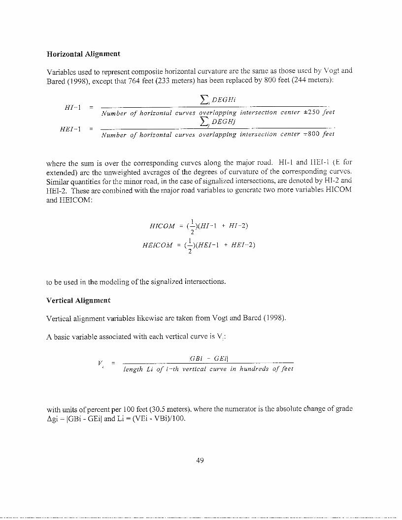
Horizontal Alignment
Vtiables used to represent composite horizontal curvature are the same as those used by Vogt andBared (1998), except that 764 feet (233 meters) has been replaced by 800 feet (244 meters):
HI- I =
HEI-I =
~1 DEGfiri
Numbev of horizontal curves overlapping intersection center +250 feet
Z, DEGh~
Number of horizontal curves overlapping intersection center +8UU jeei
where the sum is over the corresponding cuwes along the major road. El1-1 and HE 1-1 (E fo]-extended) are the unweighed averages of the degrees of curvature of the corresponding cumes.Similar quantities for the minor road, in the case of signalized intersections, are denoted by HI-2 andHEI-2. These are combined with the major road variables to generate two more variables HICOMand HEICOM:
HICOM = (:)(HI-l + H-2)
HEICOM = (~)(HEI-1 + HEI-2]2
to be used in the modeling of the signalized intersections.
Vertical Alignment
Vertical alignment variables likewise are taken from Vogt and Bared ( 1998)
A basic variable associated with each vertical curve is Vj:
v, =lGBi GEil
length Li of i -th vertical curve in hundreds of feet
with units of percent per 100 feet (30.5 meters), where the numerator is the absolute change of gradeAgi = lGBi - GEil and Li = (VEi - VBi)/100.
49
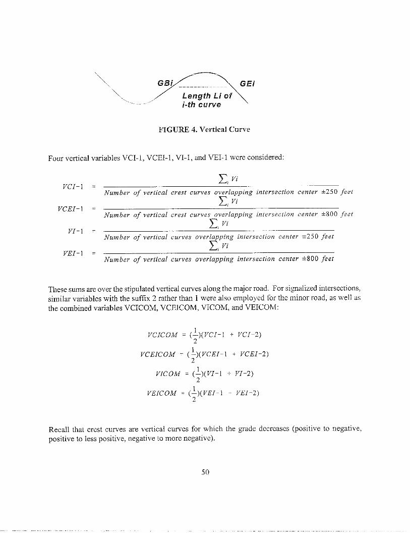
\\ ., eoy\...,,,,,
i-th curve
FIGUW 4. Vertical Ctirve
Four vetiical variables VCI- 1, VCEI- 1, VI- 1, and VEI- 1 were considered:
VCI-1 =
VCEI-1 =
VI-1 =
VEI-I =
~, Vi
Number of vertical c~est curves overlapping intersection center *2j0 feet~ Vi
Number of vertical crest curves overlapping inte~sec[ion cente? +800 feet~, vi
Number of vertical curves ove~lapping inte~section cente~ +250 feet~, Vi
Number of vertical curves overlapping intersection center *800 feet
These smsmeoverthe stipulated veflical cumesalong themajorroad. Forsignalized intersections,similar variables with the suffix 2 rather than 1 were also employed for the minor road, as well asthe combined variables VCICOM, VCEICOM, VICOM, and VEICOM:
VCICOM = (>(VCI-1 + VCI-2)
VCEICOM = (:)( VCEI-1 + 7CEI-2)L
VICOM = (#(vI-l
VEICOM = (:)(VEI - I
Recall that crest curves are vertical curves for whichpositive to less positive, negative to more negative).
50
* VI-2)
+ VEI-2)
the grade decreases (positive to negative,

Another variable developed pertaining to vertical alignment is ABSGRD 1. If only one grade wasseen on the major road, ~SG~ 1 was the absolute value of this grade. If more than one grade wa!jseen in the vicinity of the intersection on the major road, absolute values were computed of all grade!;seen at the beginnings and endings of those vertical curves that overlapped the segment of the tn]ajorroad within +800 feet (244 meters) of the intersection center. These absolute values were thenaveraged (e.g., if six grades occur corresponding to three vertical curves, their absolute values weresummed and divided by six), without regard to where they occurred (in some cases more than 800feet (244 meters) from the intersection) or the distance for which the grade remained constai.:. :4.similar variable ABSGRD2 was also developed for the minor road of signalized intersections.
Miscellaneous Variables
Driveway variables were combined to yield NODRWY1 as follows:
NODRWYI = NOD RWYRI + NO DRWYC1
and a similar combination, NODRWY2, was used for minor road driveways at signalizedintersections.
Median widths varied behveen legs of the major road in 18 out of 84 three-legged intersections, 18out of 72 four-legged intersections, and 1 out of 49 signalized intersections (most of the signalizedintersections had no median). Thus, the median width variable here, MED WIDTH 1, is the averageof the median widths of the two legs, leg 1 and leg 2, of the major road.
Speed limit variables, SPD 1 and SPD2, with values in miles per hour were assigned to the major andminor road. On the major road, SPD 1 was the average of the posted speeds on Legs 1 and 2 or theunique value seen if a posted speed was seen on only one of these legs. The same rule was appliedfor the minor road to get SPD2. In some cases, no posted speed limit was seen on the leg or legs ofthe minor road. In this case, SPD2 was assigned the default value 35.
During the modeling, it became convenient to introduce the channelization variable LTLN 1S:
1 if LTLNl is 1 OF 2LTLNIS =
O if LTLN1 is O
Yet another numerical variable was devised to denote the State:
51

O if the intersection is in CaliJ5~niaSTATE =
1 if the intersection is in Michigan
The STATE variable can be used to study whether crash experience at the various intersections isdue in part to differences between the States. Such factors as driver behavior andior crash reportingpractices may be significantly different ‘etween the t~vo States.
UNIVARIATE STATISTICS
A summ~ of the data obtained is shown in Tables 5, 6, and 7. The first item that strikes the eyeis that the mean number of crashes per intersection, no matter how they =e measured, is highest atsignalized intersections, moderate at four-legged ones, and lowest at three-legged ones.
There are a number of other ways in which the intersection classes differ. The signalizedintersections have much higher minor road ~T and much higher turning percentages than the othertwo classes. The signalized intersections tend to have more turning lanes on both major and minorlegs, and lower speed limits on the major mad as well as higher ones on the minor road. There ismore lighting on the signalized intersection, a moderate amount on the four-legged intersection, andthe least on the three-legged intersection. Likewise, the general terrain is flattest on tlhesi gnal ixedintersection, less so on the four-legged intersection, and least on the three-legged intersec~ ion. Thisis due at least in part to the fact that two-thirds of the signalized intersections are in Michigan, whi Ieonly 250/0of the other intersections are, ~d Michig~ iS a relatively flat State. The three intersectionclasses =e similar in other ways. Peak Truck Percentages at the three classes of intersections arefrom 9 to 11V. on average. There are two or three driveways per intersection on average, and theaverage value of HMRAT is from 2.2 to 2.5. Sight distances are comparable, except that signalizedintersections have a lower average sight distance left on the minor road. The signalized intersectionshave even lower sight distances left on the major road than on the minor road. This suggests thatwoods, buildings, and other obstacles are not cleared away from the minor road to the extent thatthey are from the major road.
Horizontal and vertical alignments are generally similar. Fewer of the signalized intersections,primarily in Michigan as mentioned, have horizontal curves and fewer have vertical curves.Although the average value of HEI- 1 varies substantially among the intersection classes, this averageis strongly influenced by a few intersections with sha~ turns. The average grade of signalizedintersections is a bit lower than the average for the nonsignalized intersections, and the minor roadhas a higher average grade than the major road. This phenomenon was also noted in the three-leggedand four-legged intersections, although no measurements were nlade. Frcquent]y, the minOr legsleading to an intersection on a four-lane mad have fairly steep grades as they are brought LIp or down.to confomr with the level of the major road.
52

TABLE 5. Summary Statistics: 84 Three-Legged Rural Intersections
Major road four-lane, minor leg stop-controlled, California and Michigan, 1993-1995
f~ariable and Abbreviation Min. Max. Mcdlan Mean Freq. O/OZerO
No. of Crashes TOTACC o 19 2 3.88 326 21.4
No, of Injury Crashes INJACC o 11 1 1.61 220 (67.5VO) 38.1—
No, of Intersection-Type Cmshes TOTACC1 o 13 1 2.62 135 (41.4%) 34.5
No. of Intersection-Type Injury Crashes INIACCI o 9 1 1.21 102 (31.3%) 48.8
Average Daily Traffic on Major Road ADTI, vpd 2,367 33,058 12,050 12,870
Average Daily Traffic on Minor Road ADT2, vpd 15 349 596
Peak Trock Percentage PKVoTRUCK 1.18 28.16 7.79 9.15
Peak Turning Percentage PKV”TURN 0.26 53.09 4.28 6.68.—
Peak Left-Tunr PercerrVagc PK%I.EFT 0.13 25.97 2.16 3.29
f)cak Through Percentage On Major Road pK%THRU 1 63.26 100.00 97,98 96.44
Peak Left-Turn Percentage on Major Road PK%LEFT 1 0.00 21.29 0.69 1.49 13.1
Peak Left-Tunl Pcrccntage on Minor Leg PK%LEFT2 0.00 100.00 60.99 56,64 7.1
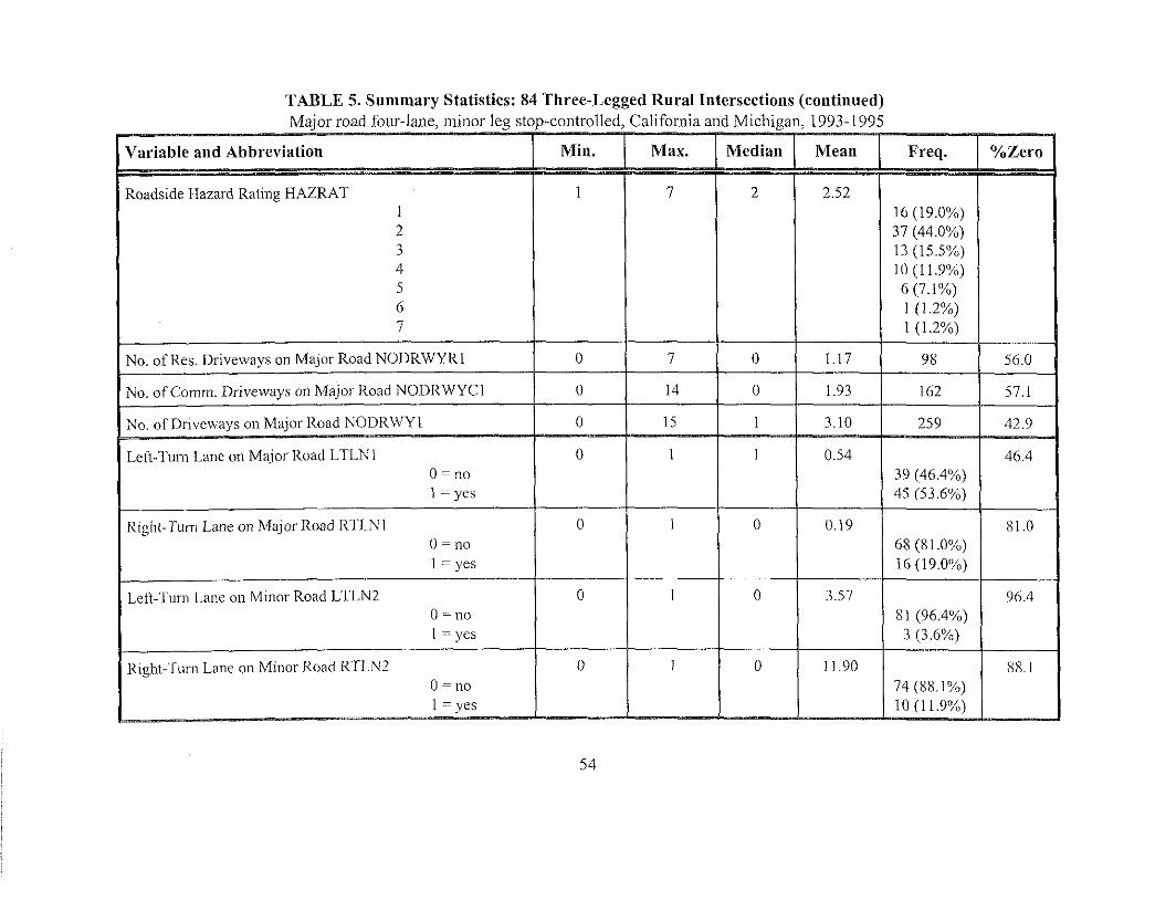
TABLE 5. Summary Statistics: 84 Three-Legged Rural Intersections (continued)Major road four-lane, n]inor leg stop-controlled, California and Michigan, 1993-1995
Variable aud Abbreviation Min. Max. Median Mean Freq. OAZero
Roadside IIazard Rating HWRK~ 1 7 2 2.52
1 16 (19.OYO)
2 37 (44.0%)
3 13 (15.5YO)
4 10 (11.970)
5 6 (7.1%)
6 1 (1 .2VO)
7 1 (1 .2YO)
No, of Res. Driveways on Major Road NOI)RWYR1 o 7 0 1.17 98 56.0
No. of Comm. I)riveways on Major Road NODRWYC1 o 14 0 1.93 162 57.1
No. of Driveways on Major Road NODRWY1 o 15 1 3.10 259 42.9
Left-’~umLane on Major”Road LTLN1 0 I I 0.54 46.4O=no 39 (46.4%)1 = yes 45 (53.6%)
Right-Tu[mLane on Major Road R1l.N I o 1 0 0.19 81.0O=nO 68 (81.OYO)1 = yes 16 (19.00A)
— ..—
Left-Turn Lane OnMinor Road LTLN2 o 0 3.57 96.4O=no 81 (96.40A)I = yes 3 (3.67.)
Right-’rorn Lane on Minor Road RTLN2 o 1 0 1).90 88.10 = 110 74 (88170)1 = yes 10 (11.9V”)
54

TABLE 5. Summary Statistics: 84 Three-I.egged Rural Intersections (continued)
Major mad four-lane, minor leg stop-controlled, California and Michigan, 1993-1995
Variable and Abbreviation Min. Max.~ Median Mean Freq. YOZero
Median Width on Major Road MEDWIDTH 1, feet o 36 0 3.74 53.6
Median Type on Major Road MEDTYPENo Median 45 (53.6V0)Painted 23 (27.4Yo)Curbed 9 (10,7%)
Other (Guardrail, Mixed, etc.) 7 (8.3%)
Angle Variable HAU, degrees -45 55 0 -0.36 83.3
Longitudinal Sight Distance on Major Road SD1, feet 500 2000+ 2000+ 1543-{-
I.eft-Side Sight Distance on Minor Road SDL2, feet 45 1399+
Right-Side Sight Distance on Minor Road SDR2, feet 80 2000+ 1375 1388+
Degt-ee of Cume HEI-1= (1/u)~ DEGHi, deg/1 00 ft o 26.6 0 2.47 52.4_— -
(“urve Grade Rate VEI-1 = (1/ln)~ (lAgi]/Li), VO/100ft o 6.71 0.04 0.89 50.0
Cres[ Grade Rate VCEI- 1 = (1/m)~ (lAgil/Li), %/100 ft o 11.0 0 0.65 59.5
A\erage Absolute Grade on Major Road ABSGRD 1, Y“ o 5.85 0.65 1.11 25.0
~
55

TABLE 5. Sulnmary Statistics: 84 Three-Legged Rural Intersections (continued)Major road four-lane, minor leg stop-controlled, California and Michigan, 1993-1995
Variable and Abbreviation Min. Max. Median nlean Freq. YOZero
Speed Limit on Major Road SPD1, mph 30 65 55 50.4
Speed Limit on Minor Road SPD2, mph 15 35 35 31.5
Light at Intersection LIGHT o = 110 52 (61 .9Vo)1 = yes 32 (38.1%)
Terrain Flat 48 (57.1 Yo)Rolling 29 (34.5%)Mountainous 7 (8.3Yo)
STATE O=CA 60 (71 .4V0)~_M1 24 (28.6°/0)
1 mph= 1.61 ktih
56

TABLE 6. Summary Statistics: 72 Four-Legged Rural IntersectionsMajor mad four-lane, minor legs stop-controlled, California and Michigan, 1993-1995
\Tariable aud Abbreviation Miu. Max. Median Meau Freq. YOZero
No. of Crashes TOTACC o 38 3.5 5.53 398 12.5
No. of Injury Crashes INJACC o 20 2 2.64 190 (47.7~0) 25.0
No. of Intersection-Type Crashes TOTACC1 o 27 2 4.13 297 (74.6VO) 22.2
No. of Intersection-TYPe Injury Crashes INJACCI o 19 1 2.19 158 (39.7%) 36.1
Average Daily Traffic on Major Road ADTI, vpd 3,350 73,000 11,166 13,018
Average Daily Traffic on Minor Road ADT2, vpd 21 2,018 410
Peak Truck Percentage PKV.TRUCK 1.70 37.24 8.36 10.95
Peak Turning Percentage PK%TURN 0.00 48.52 6.56 9.47 2.8
Peak Left-Turn Percentage PK%LEFT 0.00 25.26 6.56 9.47 2.8
Peak Through Percentage on Majol- Road PK%THRU 1 67.77 100.0 96.5 I 94.41
Peak l.eft-Tum Percentage on Majo~ Road PK%LEFT I 0.00 13.96 1.51 2.78 5.6
Peak Thl-oogh Percentage on Minol- Road PK%T11RU2 0.00 68.1 12.0 16.37 17.1
Peak Left-’I’um Percentage on Minor Road PK%LEFT2 0.00 100.00 37.5 40.58 5.7
57
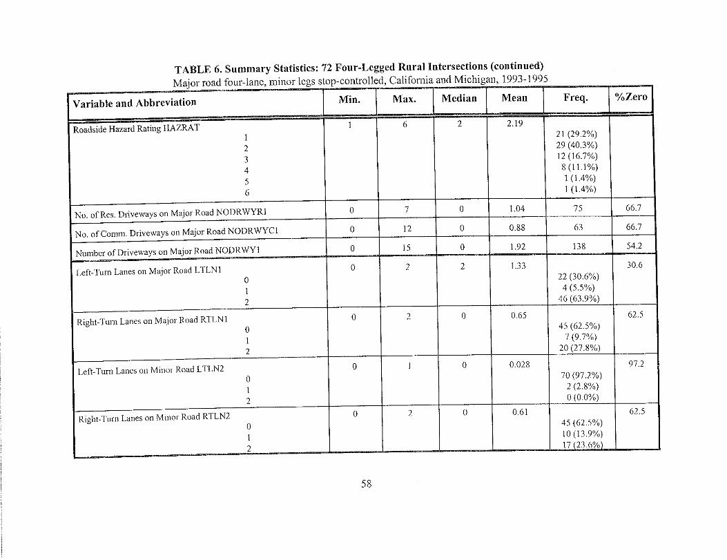

TABLE 6. Summary Statistics: 72 Four-Legged Rural Intersections (continued)Major road four-lane, minor legs stop-controlled, California and Michigan, 1993-1995
Variable and Abbreviation I Miu. \ Max. I Median I Mean I Frea. I Y.Zero.
Median Width on Major Road MEDWIDTH1, feet o 36 2 3.78 43.1
Median Type on Major Road MEDTYPENo Median 31 (43,1%)
Painted 17 (23.1%)Curbed 22 (30.6%)Other 2 (2.8 V,)
Angle Variable HAU, degrees -20 30 0 0.868 77.8
Longitudinal Sight Distance on Major Road SD1, feel 400 2000+ 1500 1430+
Left-Side Sight Distance on Minor Road SDL2, feet 324 2000+ 1438 1358+
Right-Side Sight Distance on Minor Road SDR2, feet 215 2000+ 1430 1377t
Degree of Curve HEi-i = (1/nj~ DEGHi, deg~l 00 ft o 233,3 0 5.01 56.9
Curve Grade Rate VE1-1 =(1/m)~(!Agil/Li),%/100 ft o 12.j o 0.70 61.1
Crest Grade Rate VCEI-1 = (1101)1 (lAgil/Li), ~0/loo ft o 12.5 0 0.50 75.0
Average Absolute Grade on Major Road ABSGRD 1, ‘h o j.8 0.4 0.98 38,9
1 ft = 0,305 In
59

TABI.E 6. Summary Statistics: 72 Four-Legged Rural Intersections (continued)Major road four-lane, minor legs stop-controlled, California and Michigan, 1993-1995
Variable and Abbreviation Min. Nlax. Median Mean Freq. O/OZerO
Speed Limit on Major Road SPD1, mph 25 65 55 53.68
Speed Limit on Minor Rwad SPD2, mph 25 so 35 33.35
Light at Intel-section LIGIIT O=nO 40(55,6%)
1 = yes 32 (44.4%)
Terrain Flat $9(68.1%)
Rolling 14(19,4VO)
Mountainous 9 (12.5Yo)
STATE O=CA 54 (75.OVO)
I=MI 18 (25.OYO)
1 mph= 1.61 km/h
60

TABI.,E 7. Summary Statistics: 49 Signalized Rural IntersectionsFour-legged intersections of two-lane roads, California and Michigan, 1993-1995
Variable and Abbreviation Min. Max. Median Mean Freq. Y.ZeroI
No. of Crashes TOTACC 2 48 21 20.8 1017 0.0
No. of Injury Crashes INJACC o 25 7 7.47 366 (36.OYO) 4.1
No. of intersection-Type Crashes TOTACCI 1 37 17 16.1 790 (77.7%) 0.0
No, of Intersection-Type Injury Crashes ~JACCI o 21 6 6.14 301 (29.6Yo) 4.1I
Average Daily Traffic on Major Road ADTI, vpd
Average Daily Traffic on Minor Road ADT2, vpd 940 12,478 3,670 4,367
Peak Truck Percentage PK%TRUCK 2.69 45.43 7.71 8.96
Peak Turning Percentage PK%TURN ] 7.07 I 72.66 I 34.48 I 35.64 ] IIPeak Left-Turn Percentage PK%LEFT I 4.20 I 37.07 \ 17.97 I 18.17 I IIPeak Through Percentage on Major Road PK%THRU1 I 18.01 I 96.73 ] 73.77 I 71.19 I I iPeak Left-Turn Percentage on Major Road PKY.LEFT1 [ 1.78 [ 36.67 [ 12.99 I 14.71 I IIPeak Through Percentage on Minor Road PK%THRU2 I 8.45 I 84,09 / 41.97 I 43.90 I II
Peak Left-Turn PerccnP~ge an Minor Road PK%LEFT2 2.50 75.73 24,88 28.69 I
61

TABLE 7. Summary Statistics: 49 Signalized Rural Intersections (continued)
Four-legged intersections oftwo-lane roads, California and Michigan, 1993-1995
Variable aud Abbreviation Min. Max. Median Mean Freq. YOZero
Roadside Hazard Rating HAZRAT 1 6 2 2.35
1 10 (20.4VO)
2 20 (40.8VO)
3 14 (28.6Yo)
4 3 (6.lYo)
5 1 (2.OYO)
6 1 (2.OYO)
No. of Res. D1-iveways on Major Road NODRWYR1 o 6 0 0.67 33 71.4
No. of Conlm. Driveways on Major Road NODRWYC1 o 11 2 2,35 115 32.7
No, of Driveways on Major Road NODRWY1 o 15 3 3,02 148 28.6
No. of Res. Driveways on Minor Road NODRWYR2 o 8 0 0.94 46 65.3
No. of Comm Driveways on Mirror Road NODRWYC2 o 11 3 2.24 110 22.4
No. of Driveu’ays on Minor Road NODRWY2 o 11 3 3.18 156 12.2
Left-Tunl Vanes on Major Road LTLN1 o 2 2 1.69 14.30 7 (14.3%)
1 1 (2.070)2 41 (83.77,)
Right-Turn Lanes on Major Road RrLN 1 0 2 1 0,98 42.9
0 21 (42.9VO)
1 8 (16.3 Y”)
2 20 (40.8UA)
62
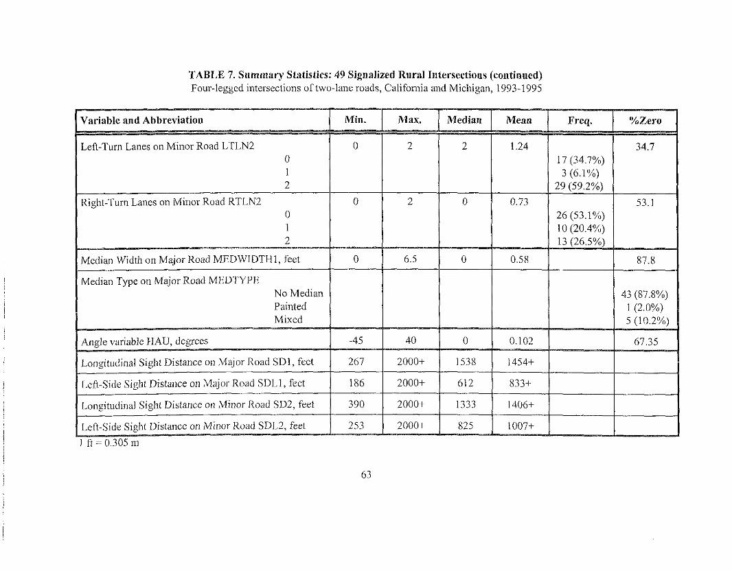
TABLE 7. Summary Statistics: 49 Signalized Rnral Intersections (continued)Four-legged intersections of two-lane roads, California and Michigan, 1993-1995
Variable aud Abbreviation Min. Max. Median Mean Freq. Y.Zero
Lefi-Tum Lanes on Minor Road LTLN2 o 2 2 1.24 34.70 17 (34.7VO)1 3 (6.170)2 29 (59.2%)
Right-Turn Lanes on Minor Road RTLN2 o 2 0 0.73 53.10 26 (53.lYo)1 10 (20,4%)2 13 (26,5%)
Median Width on Major Road MEDWIDTFI 1, feet o 6.5 0 0.58 87.8
Median Type on Major Road MEDTYPENo Median 43 (87,8%)Painted 1 (2.0%)Mixed 5 (10.2YO)
Angle variable HAU, degrees -45 40 0 0.102 67,35
Longitudinal Sight Distance on Major Road SD1, feet 267 2000+ 1538 1454+
Left-Side Sight Distance on h4ajo1-Road SDL1, feet 186 2000+ 612 833+-
Longitudinal Sight Distance on Minor Road SD2, feet 390 2000+ 1333 1406+
Lefi-Side Sigh( Distance on Minor Road SDI.2, feet 253 2000+ 825 1007+—
ft = 0.305 n]
63


Crash Data Versus Intersection Class and State
Table 8 is an extract from Tables 5,6, and 7, comparing the mean number of crashes per intersectionfor tbe tkee intersection classes. It indicates that four-legged intersections have from 1.42 to 1.81.times as many crashes as three-legged intersections. The higher ratio comes into effect as the crashseverity and the intersection-relatedness increase. This is consistent with the rough nde of thumb
TABLE 8. Mean Number of Crashes per lntersectiOn by Crash Variable and intersectionClass
three-legged four-legged signalized
TOTACC 3.88 5.53= 1.42x3.88 20.8=3.76x5.53
TOTACCI 2.62 4.13=1.58x2.62 16.1=3.90x4.13
INJACC 1.61 2.64=1.64x1.61 7.47=2.83x2.64
~JACCI 1.21 2.19=1.81x1.21 6.14=2.80x2.19
that a four-legged intersection behaves like a pair of three-ll~gged intersections, with a consequentcrash ratio of 2. Note that average major and minor road AOT’s, ~T 1 and ~T2, in Tables 5 ancl6 for three-legged and four-legged intersections, respectively, are very nearly equal, and thus tha~the comparison of three-legged and four-legged intersections is j ustifiable.
Whh regad to the signrrlized intersections, Table 8 indicates that they have from 3.90 to 2.80 timesas many crashes as four-legged intersections. These two intersection classes have in common four-leggedness, but otherwise are quite different (lanes, control, and ~T)I. Nonetheless, it appears thatintersection-relatedness, i.e., all crashes versus those satisfi]ing the BMI criteria (see p. 40), has anegligible effect on the crash ratio, but that the fraction of serious crashes is lower at signalizeciintersections than it is at the four-legged intersections.
Table 9 provides a decomposition of crashes by seventy and State for the three intersection classes.Whh respect to State, it indicates that lMichigan crashes tend to be less severe than Cali fomia crashesfor all classes, regardless of intersection-relatedness. Regardless of State, signalized intersectionshave the lowest percentage of serious crashes and four-”legged intersections have the highestpercentage. Intersection-related crashes (TOTACCI) have a slightly higher tendency to be seriou!]than all crashes (TOTACC) for both States and all three intersection classes.
The data in Table 9 are represented in another way in Table 10. Table 10 indicates that CaIifomi~is rmderrepresented in crashes in both the four-legged and si[inalized intersectiOn samples and pafib{underrepresented in the thee-legged intersection sample. It also shows that such under-representation decreases for serious crashes and that for the three-legged intersections, Cali fomi ais ovemepresented in serious crashes. The modeling later in this report will attempt to sort out
65
BIVAWATE STATISTICS
To prepare for model development, it is appropriate to ask what variables correlate strongly withcrash counts and to note the mutual correlations of highway variables with one another.
In the tables that follow, correlation coefficients between variables are shown, along with P-values,for each of the three data sets. Recall that the P-value is the estimated probability that the measuredcorrelation coefficient would be at least as far from 2 as it is found to be if the true cor!-ciatioiicoefficient for the population from which the sample is drawn is zero. A small P-value indicates thata correlation is significant, a large one indicates that no particular significance can be attached to it.The correlation coefficient summarizes the sample: if it is positive, the variables compared tend toincrease together in the sample; if it is negative, they tend to decrease together. If the correlationcoefficient is fa from zero and its P-value is small, the sample is unlikely to have been drawn froma population where the true correlation is zero; if the correlation coefficient is close to zero and itsP-value is large, the sample resembles a sample drawn randomly from a population whose overailcorrelation coefficient is zero.
Other cautions should be offered in the interpretation of comelation coefficients, If a variablecorrelates strongly with, say, number of crashes, it may be that the variable is not in itself influential.but that it happens to correlate strongly with another variable that is influential. Likewise, if avariable seems to have a weak correlation with the number of crashes, it may be in part because theinfluence of the variable is masked by the presence of other more influential variables. The poinlof modeling is to determine the leading influences and then discover secondary influences, e.g.,crashes may be strongly dependent on ADT, but after ADT is properly taken into account, theresidual, the portion of crash count that cannot be expressed in terms of ADT, may be stronglycorrelated with another variable.
Crashes Versus Other Variables
TabLes 11, 12, and 13 exhibit correlation coefficients and P-values between crash courr!s and othervariables for the three data sets.
Table 11 exhibits the correlations between intersection crashes and highway variables for the three-
legged intersections. Major and minor road ADT’s correlate positively with crashes, as expected.Peak turning percentages also correlate with crashes, both positively and negatively. Since theseturning percentages correlate with each other, it is not immediately clear what the chief influenceare. mile HAZRAT is insignificant, number of driveways correlates positively with crashes andmedian width correlates negatively; neither result is unexpected. The angle variables HAU and DEVare both significant, with HAU more so than DEV. The sign, however, is no[ what the Kulmal](1995) study suggests, but it is consistent with the work of Vogt and Bared ( 1998) for three-leggedintersections. Sight distance is not significant, although minor road sight distance left is nrarginall:ysignificant. Both left and right turns from the minor road are affected by sight distance left. Thehorizontal variable HEI- 1 and the vertical variables VI-1 and VEI- 1 are significant. LIGHT and
67
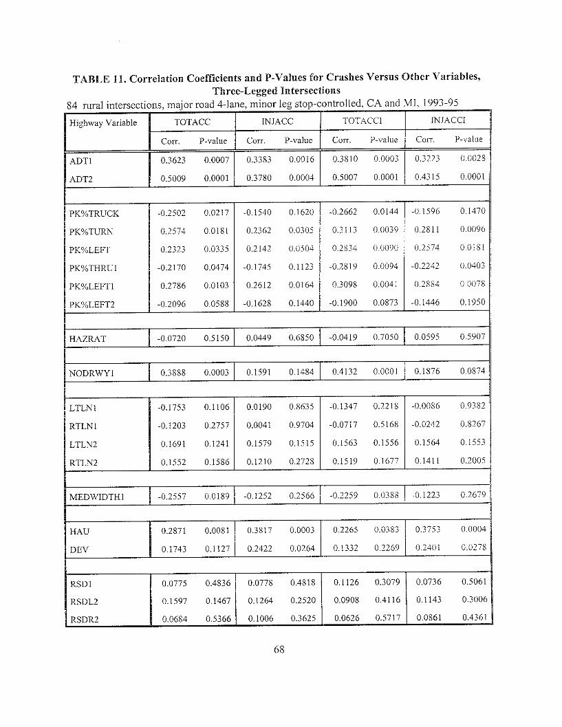
TABLE 11. Correlation Coefficients and P-Values for Crashes Versus Other Variables,Three-Legged Intersections
84 rural intersections, major road 4-lane, minor leg stop-controlled, CA and MI, 1993-95
Highway Variable TOTACC INJACC TOTACC1 lNJ.4CCI
COrr. P-value CoII. P-value CoI-r. P-valtle COrr. P-vah]e
ADT1 0.3623 0.0007 0.3383 0.0016 0.3810 0.0003 0.3223 0.002E
ADT2 0.5009 0.0001 0.3780 0.0004 0.5007 0.0001 0.4315 0.0001
PK%TRUCK
PK%TURN
PKY”LEFT
PK%THRU1
PKV”LEFT1
PKYOLEFT2
-0.2j02 0.0217
0.2j74 0.0181
0.2323 0.0335
-0.2170 0.0474
0.2786 0.0103
-0.2096 0.0588
-0.1540 0.1620
0.2362 0.030j
0.2142 0.0504
-0.174j 0.1123
0.2612 0.0164
-0.1628 0.1440 r-0.2662 0.0144 -(). 1596 0.147C
0.3113 0,0039 ().2X1 1 0.0096
().2X34 ().0()9() 0.2574 OOIXI
-0.2X19 0.0094 -0.2242 0.0403
0.3098 0.0041 0.28X4 () ()()78
-0.1900 0.0873 -0.1446 0.1950
HAZRAT -0.0720 0.5150 0.0449 0.6850 -0.0419 0.7050 0.0j95 0.5907
NODRWYI 0.3888 0.0003 0.1591 0.1484 0.4132 0.0001 0.1876 0.0874
“>TLN 1 -0.1753 0.1106 0.0190 0.863j -0.1347 0.2218 -0.0086 0.9382
%TLN1 -0.1203 0.2757 0.0041 0.9704 -0.0717 0.516X -0.0242 0.X267
rrLN2 0.1691 0.1241 0.1579 0.lj15 0.1563 0.1556 0.1564 0.1553
%TLN2 0.lj52 0.lj86 0.1210 0.2728 0.1519 0.1677 0.1411 0.2005
MEDWIDTHI -0.2557 0.0189 -0.1252 0.2j66 -0.2259 0.03XX -0.1223 0.2679
HAU 0.2871 0.0081 0.3817 0.0003 0.2265 0.0383 0.3753 0.0004
DEV 01743 0.1127 0.2422 0.0264 0.1332 0.2269 0.2401 0.027X
RSD 1 0.0775 0.4836 0.0778 0.4818 0.1126 0.3079 0.0736 0.5061
RSDL2 0.1597 0.1467 0.1264 0.2520 0.0908 0.4116 0.1143 0.3006
RSDR2 0.0684 0.5366 0.1006 0.3625 0.0626 0.5717 0.0X61 0.4361
68

TABLE 11. Correlation Coefficients and P-Values for Crashes Versus Other Variables,Three-Legged Intersections (continued)
84 rural intersections, major road 4-lane, minor leg stop-controlled, CA and MI, 1993-95
1
Highway Variable TOTACC INJACC TOTACCI INJ.ACC1 !
Corr. P-value Corr. P-value COrr. P-value Corr. P-value
HI-1 0.0552 0.6181 0.0834 0.45J7 0.0489 0.6590 0.0753 o,~~j~
HEI- 1 0.2366 0.0303 0.1786 0.1041 0.1946 0.076) 0.1676 0.1275
VI- 1 0.1742 0.1131 0.1614 0.1426 0.2437 0.02jj 0,2287 0.0364
VEI. 1 0.1673 0.1283 0.1530 0.1647 0.2208 0.0436 0.2060 0.0601
VCI- 1 0.0251 0.8210 0.0513 0.6429 0.0637 0.5647 0.0676 0.5410
VCEI- 1 0.1321 0.2308 0.1234 0.2633 0.1774 0.106j 0.1922 0.0799
ABSGRD 11
0.0099 0.9288 0.1158 0.2942 0.0492 0.6567 0.0931 0.3997
SPD 1 -0.3688 0.0006 -0.1314 0.2334 -0.350Y 00011 -0.1591 o.14x3
7PD2 -0.1133 0.3047 0.0174 0.8753 -0.0208 0.8513 0.0664 0.5483
,lGHT 0.3290 0.0022 0.2163 0.0481 0.3242 0.0026 0.2078 0.0579
;TATE 0.1459 0.1853 -0.0823 0.4568 0.0327 0.7680 -0.1054 0.3402
major road speed (SPD 1) correlate positively and negatively, respectively, with crashes, but they alsocorrelate positively and negatively, respectively, with minor road ADT (cf. Table 15), and thismay be an exmple of one variable representing another. The same applies to Peak TruckPercentage, which correlates negatively with both crashes md ADT (Tables 11 and 15). Thevariable STATE does not seem to play an important role in three-legged intersection crashes.
In Table 12, similar correlations are found between crashes on. four-legged intersections md highwayvariables. ADT1 is a bit less significant than in the three-legged case. Peak turning percentagescorrelate with crashes, but the minor road turning percen~ages are less significant. HAZRATremains insignificant, but now it is joined by number of driveways and median width, which are alsc,
insignificant. The typical Huard Rating and number of driveways at foLlr-iegged iIllcrsect iOIISarc
69
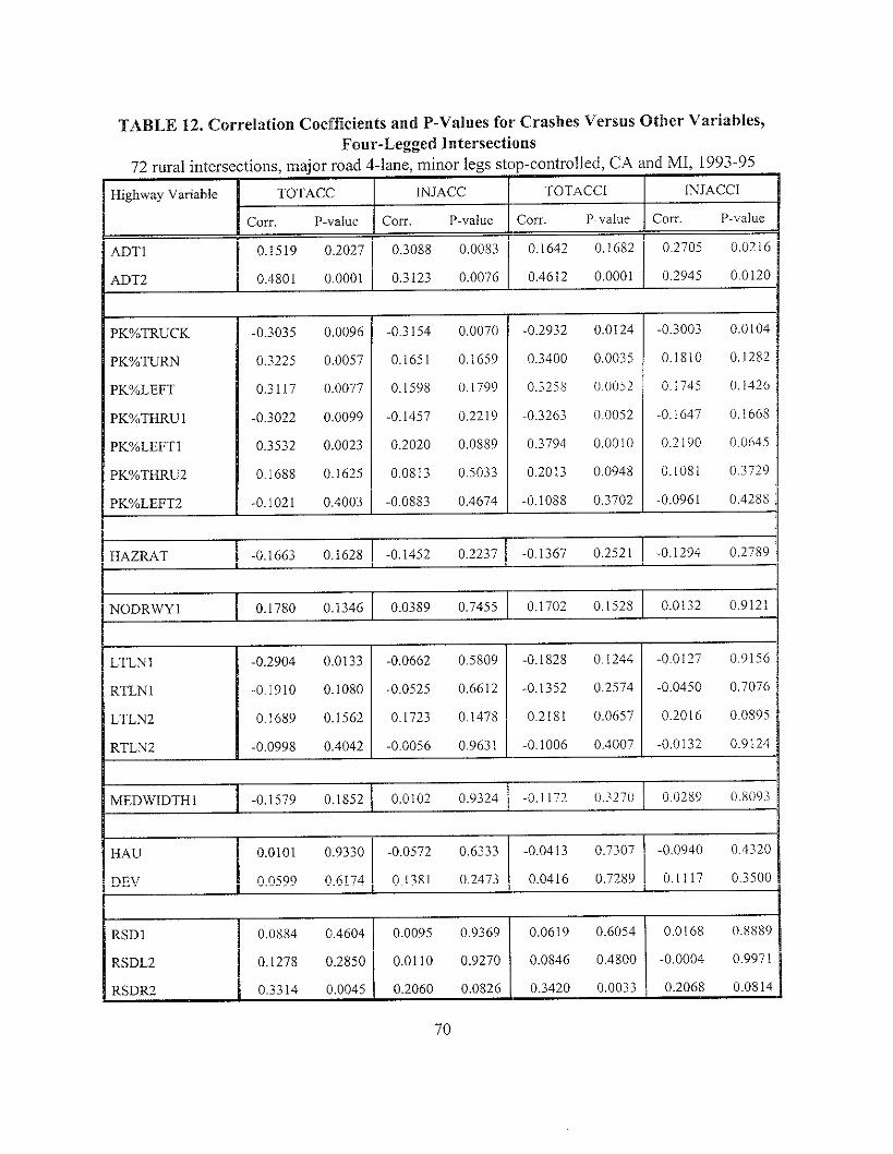
TABLE 12. Correlation Coefficients and P-Values for Crashes Versus Other Variables,Four-Legged Intersections
72 mral intersections, major road 4-lane, minor legs stop-controlled, CA and MI, 1993-95
HighwayVariable1
TOTACC INJACC TOTACC1 IhJACCI
COrr. P-value Corr. P-value con. P-value con. P-\,alue
ADT1 0.1519 0.2027 0.3088 0.0083 0.1642 0.1682 0.270j 0.0216
ADT2 0.4801 0.0001 0.3123 0.0076 0.4612 0.0001 0.2945 0012(
PKYoTRUCK
PK%TURN
PKY”LEFT
PK%THRU1
PK%LEFT1
PKYOTHRU-2
PKY.LEFT2
B
-0.3035 0.0096
0.3225 0.0057
0.3117 0.0077
-0.3022 0.0099
0.3532 0.0023
0.1688 0.1625
-0.1021 0.4003
I
-0.3154 0.0070
0.1651 0.1659
0.1598 0.1799
-0.1457 0.2219
0.2020 0.0889
0.0813 0.5033
-0.0883 0.4674
-0.2932 0.0124
0.3400 0.0035
0.3258 0.00j2
-0.3263 ().0052
0.3794 0.0010
0.2013 0.0948
-0.1088 0.3702
-0.3003 0.0104
0.1810 0.1282
0.174j 0.142C
-0.1647 0.1668
O.zlgo 0.0645
0.1081 0.3729
-0.0961 0.4288
HAZRATI
-0.1663 0.1628 -0.1452 0.2237 I -0.1367 0.2j21 -0.1294 0.2789
VODRWY11
0.1780 0.1346 0.0389 0.7455 0.1702 0.lj28
:TLN1
lTLN 1
LTLN2
KTLN2
0.0132 0.9121
-0.0127 0.91j6
-0.0450 0.7076
0.2016 0.0895
-0.0132 0.9124
MEDWIDTH 11 -0.1579 0.1852 0.0102 0.9324 -0.1172 (1..727(1 0.0289 0.8093
HAU 0.0101 0.9330 -0.0572 0.6333 -0.0413 0.7307 -0.0940 0,4320
DEV 0.0599 0.6174 0.1381 0.2473 0.0416 0.7289 0.1117 03500
RSD 1 0.0884 0.4604 0.0095 0.9369 0.0619 0.6054 0.0168 0.8889
RSDL2 0.1278 0.2850 0.0110 0.9270 0.0846 0.4800 -0.0004 0.9971
RSDR2 0.3314 0.0045 0.2060 0.0826 0.3420 0.0033 0.2068 0.0814
70

TABLE 12. Correlation Coefficients assd P-Values for Crashes Versus Other Variables,Four-Legged Intersections (continued)
72 rural intersections, major road 4-lane, minor legs stop-controlled, CA and MI, 1993-95
HighwayVariable TOTACC lNJACC TOTACC1 INJACC1
HI- 1
COrr. P-value con. P-\alue Corr. [>-value CoI-r. p-valLl~
0.0396 0.7411 -0.0740 0.5366 -0.0139 0.908 I -0.0487 0.6848
HE1-1 1 -0.0423 0.7240 -0.0481 0.6880 -0.0829 0.4890 -0.0762 0.j249
VI- 1
VEI- 1
VCI- 1
VCEI- 1
&BSG~l I -0.0177 0.8826 -0.0332 0.7822 I -0.0012 0,9918 -0.0140 0.9073
jPD 1 -0.2753 0.0193 -0.0306 0.7988 -0.2477 0.03j9 -0.0007 0.9957
jPD2 -0.0778 0.5158 0.2541 0.0312 -0.0006 0.9963 0.2742 0.0197
LIGHT 0.0393 0.7430 -0.0377 0.7j33 -0.oloj ().9303 -0.0633 ().5<176
3TATE
slightly less than they are at three-legged intersections, and this perhaps is relevant. However,median width, on average, is as Iligh at four-legged intersections as at three-legged intersections,with a lower percentage of zero medians at four-legged intersections. Four-1egged geometries,perhaps, lessen the safety effect of medians.
As with the three-legged intersections, major road turning lanes tend to decrease the number o fcrashes (or are insignificant for injury crashes), while minor road turning lanes increase the numberof crashes or are insignificant. In the three-legged case, minor road turning lanes correlate strongl]twith minor road ~T, but this is not true for four-legged intersections. Peak truck percentage stillcorrelates negatively with crashes and positively with ADT (Table 16), but LIGHT, which there i:jmore of on the four-legged intersections, is now insignificant.
Neither angle variable HAU or DEV is significant on the fOur-legged intersections. perllaPs this is
71

TABLE 13. Correlation Coefficients and P-Values for Crashes Versus Other Variables,Signalized Intersections
49 signalized 4-legged mral intersections, 2-lane by 2-lane roads, CA and .MI, 1993-95
Highway Variable TOTACC INJACC TOTACC1 INJACCI
con. P-value Corr. P-value con. P-value COrr. l>-,allie
ADT1 0.0166 0.9099 o.03jo 0.8219 0.0686 0.6393 0.0537 0.7138
ADT2 04490 0.0012 0.1020 0.4857 0.3873 0.0060 0,0392 0.7893
PK%TRUCK 0.2675 0.0631 0.4431 0,0014 0.2760 0.0549 0.4308 0.0020
PKVOTURN 0.2110 0.14j7 0.0147 0.9202 0.1496 0.3049 -0.0642 0.661j
PKYoLEFT 0.2175 0.1333 0.0022 0.9879 0.1489 0.3071 -0.0801 0.5845
PKYoTHRU 1 -0.2693 0.0614 -0.0660 0.6524 -0.2472 0.0868 -0.0086 ().9j33
PK%LEFT1 0.3j57 0.0121 0.1521 0.2967 0.3507 0.0135 0.1450 0.3203
PK%THRU2 0.1482 0.3096 0.1176 0.4210 0.1996 0.1692 0.1686 0.2468
PK%LEFT2 -0.3230 0.0236 -0.2526 0.0800 -0.3629 0.0104 -0.3101 0.0301
HAZRATI
0.0136 0.9260 0.0890 0.5433 0.063 I 0.6667 0.1462 0.3163
NODRWY1 0.4005 0.0044 0.1823 0.2099 0.3641 0.0101 0.1021 0.4852
NODRWY2 0.0255 0.8618 0.0179 0.9028 0.0331 0.8212 0.0014 0.9924
LTLN 1 -0.2046 0.1584 -0.0058 0.9683 -0.1022 0.4849 0. I088 0.4j69
RTLN 1 -0.1107 04490 -0.0728 0.6194 -0.1085 0.4582 -0.0824 0.5737
>TLN2 -0.1755 0.2277 -0.0760 0.6037 -0.1838 ().2062 -0.0688 0.6387
LTLN2 0.2425 0.0932 0.1363 0.3j04 0.2216 0.1260 0.1301 0.3730
MEDWIDTH1I
-0.0394 0.7882 -0.0216 0.8827 00190 0.8968 0.0401 0.7843 !
HAU -0.0070 0.9610 0.0079 0.9j71 0.0535 0,71j3 0.0j33 0.7163
DEV -0.0587 0.6886 -0.1496 0.3051 -0.0874 0.5504 -0.1639 0.260j
72

TABLE 13. Correlation Coefficients and P-Values for Crashes Versus Other Variables,Signalized Intersections (coi~tinued)o
49 signalized 4-legged mral intersections, 2-lane by ~
Highway Variable TOTACC INJACC
Corr. P-value Col-r. P-value
-0.1129 0.4401 -0.0403 0.7832
RSDL 1 I -0.2085 0.1505 -0.1310 0.3695
RSD2 ~ 0.0079 0.9j71 I -0.0165 0.9104
RSDL2 1-0.0615 0.67491-0.0829 0.5713
lane roads, CA and MI, 1993-95
TOTACCT INJACCI
con. P-value COrr. P-value
c
HI- 1 -0.2232 0.1232 -0.1936 0.1825 -0.2398 0.0970 -0.1815 0.2120
HEI- 1 -0.0152 09177 -0.0892 0.5421 -0.0651 0.6j67 -0,1457 0.3178
HI-2 .0,2391 0.0980 -0.2039 0.1601 -0.2230 0.1236 -0.1867 0.1990
HEI-2 -0.1749 0.2295 -0.1540 0.2907 -0.1487 0.3079 -0.1363 0.3503
HICOM -0.3268 0.0219 -0.2815 0.0501 -0.3317 0.0199 -0.2613 0.0697
HEICOM -0.0817 0.5766 -0.1434 0.3258 -0.1186 0.4169 -0.1897 0.1918
VI- 1
VEI- 1
VC1- 1
VCEI- 1
VI-2
VEI-2
VCI-2
VCEI-2
VICOM
vEICOM
VCICOM
VCEICOM
0.0634 0.6654
0.2196 0.1294
0.1942 0.1811
0.0465 0.7511
0.1356 0.3531
0.1486 0.3081
0.1065 0.4663
0.1472 0.3127
[0.1417 0.3316
0.2188 0.1310
0.1633 0.2621
0.1534 0.2927
0.0277 0.8504
0.1316 0.3674
0.1029 0.4818
0.0069 0.9627
0.0931 0.5246
0.1038 0.4778
0.0355 0.8086
0.0875 0.5501
I0.0903 0.5372
0.1437 0.3245
0.0676 0.6442
0.081j 0.5779
73
0.0113 0.9386
0.1631 0.2627
0.0782 0.5933
0.0069 0.9626
0.1388 0.3417
0.1524 0.2957
0.0988 0.4993
0.1466 0.3147
I
0.0510 0.7230
0.0891 0.5429
0.0302 0.8368
-0.0j49 0.7082
0.1 29j 0,37j2
0.1353 0.3541
0.0729 0.6187
0.1217 0.4050
0.1214 0.4061 0.131j 0.3677
0.1985 01715 0.1530 0.2938
0.1163 0.4263 0.0762 ().(,026
0.1345 0.3570 I 0.0834 0.5687

TABLE 13. Correlation Coefficients and P-Values for Crashes Versus Other Variables,Signalized Intersections (continued)
49 signalized 4-legged rnral intersections, 2-lane by 2-lane roads, CA and MI, 1993-95
HighwayVariable TOTACC INJACC TOTACC1 lXJACC1
Corr. P-value COrr. P-value Corr. P-value Corr. I>-value
ABSGRD1 0.0328 0.8228 -0.0365 0.8032 0.0269 0.8545 -0.0445 0.7614
ABSGRD2 -0.0822 0.5744 -0.0316 0.8294 -0.1005 0.4920 -0.0461 0.7530
SPD 1 -0.1201 0.4111 0.1354 0.3538 -0.0744 0.6112 0.2006 0.1670
SPD2 0.0246 0.8668 0.2031 0.1616 0.0960 0.5118 0.2816 0.0499
PROT_LT -0.2925 0.0414 -0.0767 0.6006 -0.1242 0.395 I o.030- ().s.340
LIGHT -0.1336 0.3601 -0.0670 0.6473 -0.0619 0.6729 -0.0827 0.5723
STATE 0.3690 0.0091 0.1817 0.2115 0.1977 0.1732 0.0481 0.7429
because they are less variable on the four-legged intersections than on the three-legged intersections,with standard deviations on the three-legged intersections being aboot twice what they are on thefour-legged intersections. Minor road sight distance right is significant on the fear-l eggec!intersections, an indication that left-turn and through traffic on the minor mad may have a greatertendency toward crashes than right-turn trafbc. All remaining alignment variables, including grade,are insignificant .on the four-legged intersections. STATE appews to be significant for fOur-leggetlintersections, and this is consistent with Table 10.
Correlation coefficients of crashes with other variables for the signalized intersections are shown inTable 12. Remarkably, ADT1 is insignificant, and ADT2 is insignificant fOr injuv crashes. Thisis perhaps due to the relatively small sample size and the presence of a variety of other influentialfactors. Peak Trock Percentage, which negatively correlates with ADT (cf. Table 16), altbooghweakly, has a strong positive correlation with crashes. Peak tLlming percentages have somesignificant correlations, positive and negative, with crashes, and they wi II be examined more c Iosel>,later in this chapter. HAZRAT, channelization, median width, and the angle variables are generallj
insignificant. Median widths are mostly zero, but HAU and DEV, the angle variables, are aboLlt asvariable as in the three-legged intersections and still have a.negligible effect. Sight distances andhorizontal alignment are generally insignificant with the wrong sign. This indicates that when otherfactors are ignored, shorter sight distmce and more horizontal curvature lead to fewer crashes. Onthe other hand, vertical alignment, although generally insignificant, h~s the right sign: other factorj
74

ignored, crashes rise with more grade change per unit distance. Speeds, though genetall!~
insignificant, seem to correlate positively with injury crashes. The existence of a protected left turn,which correlates positively with major mad ADT, correlates negatively with crashes, as one mightexpect. This may, in pall, account for the poor showing of ADT 1. Finally, LIGHT is insignificant.but STATE shows a positive correlation with crashes.
As a general rule, correlations are similar for TOTACC and TOTACCI, and for INJACC andINJACC1. However, there are significant differences as one passes fronl all crashes to seriouscrashes (from TOTACC to NJACC, or from TOTACCI to INJACCI). Items that stand out includethe following:
. ADT1 and ADT2 are both significant at three-legged and four-legged intersections, withADT2 generally more significant; but at the signalized intersections, neither is signi fican!except ADT2 with TOTACC and TOTACCI.
. PKYoTRUCK correlates negatively with crashes of all types at three-legged and four-leggedintersections and positively at signalized intersections.
o Peak tming percentage variables correlate strongly with crashes of all types at three-leggecland four-legged intersections, and with TOTACC and TOTACCI at signalized intersections.
. NODRW1 correlates positively with TOTACC and TOTACCI at all intersection types, bu[correlates insignificantly with lNJACC and INJACCI at four-legged and signalizedintersections.
. LMEDWIDTH1 correlates negatively with TOTACC and TOTACCI at three-legged and four-legged intersections, but insignificantly with INJACC and TNJACCI.
. Channelization variables correlate less significantly with lNJACC and fNJACC I than witbTOTACC and TOTACCI and sometimes have correlation coefficients ofunexpec[ed sign.
o HAU and DEV correlate strongly with all crash types at three-legged intersections
e Sight distance variables generally have insignificant correlation, except for RSDR2 at four-legged intersections, which correlates positively with all crash types.
. Horizontal alignment variables have insignificant correlation andlor correlation coefficientwith unexpected sign, except for HEI- 1 at three-legged intersections, while HICOklcorrelates negatively with all crash types at signalized intersections (fewer crashes atsignalized intersections with major or minor road horizont~l curves out to 250 feet (76meters)).
75

. Vertical alignment variables are insignificant arrd/or have correlation of unexpected sign,except for VI-1 and VE1-I at three-legged intersections and VETCOM at signalizedintersections, the effect being stronger for TOTACC and TO~ACC 1than for INJACC andINJACCI.
. SPD 1 correlates negatively with TOTACC and TOTACCI at ‘!hree-legged and fou--leggedintersections; SPD2 correlates positively with INJA.CC and [NJACCI at four-legged andsignalized intersections.
o LIGHT correlates positively with all crash types at three-legged intersections
e STATE correlates positively with TOTACC and TOTACCI at four- ]egged and signalizedintersections.
. PROT_LT correlates negatively with TOTACC, but nOt sigli ficalltly with INJACC andINJACCI for signalized intersections.
Information pertaining to TOTACC is summarized in Table 14. Featores not already mentioned thatare related to TOTACC include:
. ADT1 has lessened significance as one passes from three-legged to four -iegged to signalizedintersections.
. LIGHT correlates positively with TOTACC at three-legged and four-legged intersections(perhaps because lights are placed at high crash locations).
. LTLNI correlates negatively with TOTACC on all three data sets
. At three-legged intersections, HEI- 1 and RSDL2 correlate positively with TOTACC.
. At four-legged intersections, horizontal and vertical variables have correlation coefficientsof mixed signs with TOTACC, while all sight distances have coefficients of appropriatesigns, with RSDR2’S being significant.
. At signalized intersections, vertical variables have positive correlation with TOTACC,horizontal variables have negative correlation, and sight distance variables have mixedcorrelation.
ADT and State Versus Other Variables
It is generally recognized that ADT is the most important explanatory variable in modeling crashesIt is therefore appropriate to make a special effort to determine when other variables are correlatedwith ADT so that one can begin to distinguish effects that are properly due to these variables apafl:
76

TABLE 14. Correlates of T~3TACC
84 Three-legged Intersections
Positive correlates Negative correlates Insignificant correlates
ADT1*, ADT2* PKVOTRUCK* PKOARIGHTl
PKVO~RN*, PKYoLEFT* PK%THRU1 * HAZRKi (neg)
PKVOLEFT1* PK%LEFT2* (82 int.) RTLNI (neg)
PKY.RIGHT2” (82 int.) MEDWIDTHI * RSD1 , RSDR2
NODRWY1*,HAU*> DEV* SPD1* HI- 1
HEI- 1*. LIGHT* LTLN1 VCI- 1, VCEI- 1
LTLN2;RTLN2,R SDL2 ABSGRD I
VI- 1, VEI- 1, STATE SPD2(neg)
72 Four-1egged Intersections
Positive correlates
ADT2*PK%TURN*PKVOLEFT*, PKVOLEFT1 *PKVOWGHT1*RSDR2*, STATE*PKV~THRU2(70illt.)NODRWY1,LTLN2ADT1 (P-value= 0.2027)
Positive correlates
ADT2*,PKYOTRUCK *
PK%LEFT1*
NODRWY1*,
NODRWYCOM*
F:*, F,*>STATE*
RTLN2*>PK%TURN
PK%LEFT,VCI- l,VEI-1
VEICOM
3Negative correlates Insignificant correlates
PK%TRUCK* PK%LEFT2, PKV,RIGHr2PKV”THRU1* (both neg., 70 int.)LTLN1 * RTLN2(neg),HAU, DEVSPD 1“ RSD1,RSDL2,HI-1
HAZUT HEI-1 (neg), VI-I (neg)
RrLNl VEI-l(neg),VCI- l(neg)MEDWIDTHI VCEI-l,ABSGRDI (neg)
SPD2(neg),LIGHT
49 SiWalized Intersections
Negative correlates
PKO/OTHRUl”PK”hLEFT2*PROT_LT*HI-2*, HICOM”, HI-1LTLN1,RSDL1
[insignificant” means P-value in excess Of O.20, “*” mea]
Insigllil’iciilll c<)rrelatcs
ADT1,l’,, F2,PKVORIGHTIPKVOTI+RU2, PK%RIGHT2HAZRAT,NODRWY2LTLNl,RTLNl(neg)MEDWIDTHl(neg)I-IAU,DEV(bOth neg)RSDl,RSDL2(b0th neg), RSD2HEI- 1, HEI-2 (both neg)HEICOM (neg)VI-1, VCEI-1VI-2, VC1-2, VEI-2, VCEI-2,VICOM,VCICOM, VCEICOMABSGW31,ABSGRD2 (neg)
SPD 1 (neg), SPD2, LIGHT (Ileg)
P-value less thm 0.10
77

TABLE 15. Correlation Coefficients and P-Values for ADT and STATE VersusIntersection Variables, Three-Legged Intersections
84mralintersectiolls, major road4-lme, minor legstop-control! ed, CAand MI, 1993-95
Highway ADT1 ADr2 STATEVariable
Corr. P-value Corr. P-value Corr. P-value
ADT1 1.0000 0~1612 0.1429 -0.1156 0.2951
ADT2 0.1612 0.1429 I .0000 0.0000 0.2240 ().0406
STATE 1 -0.1156 0.2951 0.2240 0.0406 I 1.0000 0.0000
PKYoTRUCK
PK%TURN
PK%LEFT
PK%THRUI
PKYoLEFT1
PK%LEFT2
-0.2349 0.0315
-0.1079 0.3286
-0.1319 0.2317
0.1024 0.3540
-0.0353 0.7500
-0.2709 0.0138
-0.2211 0.0433
0.6842 0.0001
0.6658 0.0001
-0.6183 0.0001
0.6404 0.0001
-0.1145 0.3058
-0.0993 0.3686
0.0251 0.8208
0.0530 0.6323
0.0213 0.8477
0.0132 09052
-0.0380 0.7345
HURAT 1 0.1405 0.2025 I -0.1416 0.19901 -0.4795 0.0001
NODRWY1 0.1347 0.2217 0.2166 0.0478 0.242j 0.0262
.TLNI
ZTLN1
;TLN2
lTLN2
0.2027 0.0644
0.2585 0.0176
0.0195 0.8601
-0.1127 0.3076 -0.6794 0.()()(11
-0.0218 0.8442 -0.3067 0.0045
0.4336 0.0001 -0.1217 0.2701
0.0311 0.7786 0.2513 0.0211 0.1744 0.1127
MEDWIDTH1 1 0.0251 0.8211 \ -0.2267 0.0381 -0.3923 0.0002
HAU -0.0164 0.8823 0.1250 0.2574 0.2042 0.0624
DEV 0.0992 0.3691 0.0418 0.7056 -0.0654 0.5545
79

TABLE 1S . Correlation Coefficients and P-Values for AD’~ and ST.4TE VersusIntersection Variables, Three-Legged Intersections (continued)
84rural intersections, major road 4-lane, nlinorleg stop-control! ed, CAalld MI, 1993-95
Highway A.DT1 AD7:2 STATEVariable
Corr. P-value cm-r. P-value Corr. P-value
RSD 1 0.2673 0.0140 0.0576 0.6030 0.0280 0.8003
RSDL2 0.1149 0.2998 -0.0424 0.7020 -0.0923 0.4038
RSDR2 0.1339 0.2248 0.0034 0.9755 -0.0818 0.4597
HI- 1 0.0765 0.4892 0.0214 0.8472 -0.0258 0.8160
HEI- 1 0.1326 0.2294 0.0347 0.7540 0.1134 0.3043
VI-1
VEI- 1
VCI- 1
VCEI-1
0.2868 0.0082 0.0772 0.4852 -0.0484 0.0623
0.2501 0.0218 0.0509 0.6455 -0.0471 0.6706
-0.0203 0.8545 -0.0719 0.51j9 0.1620 0.1410
0,1607 0.1442 0.0854 0.4401 0.0467 0.6733
ABSGRD1 I 0.1299 0.2389 I -0.0680 0.5387 \ -0.3052 0.0048
SPD 1 -0.0703 0.5250 -0.2895 0.0076 -0.4397 0.0001
SPD2 0.0375 0.7348 -0,1394 0.2061 -0.7916 0.0001
LIGHT I 0.0917 0.4070 I 0.3625 0.0007 I 0.3178 0.0032
80

TABLE 16. Correlation Coefficients and P-Values for AW~and STATE VersusIntersection Variables, Four-Legged Intersections
72 rural intersections, major road 4-lane, minor legs stop-controlled, CA and MI, 1993-95
Highway ADT1 ADT2 STATEVariable
Corr. P-value Corr. P-value Col-1-. P-value
ADT1 1.0000 0.0000 -0.1083 0.3653 -0.1436 0.2288
ADT2 -0.1083 0.3653 1.0000 0.0000 0.4082 0.0004
STATE 1 -0.1436 0.2288 0.4082 0.0004 1.0000” 0.000c
PKYoTRUCK
PKYoTURN
PK%LEFT
PKYoTHRU1
PK%LEFT1
PK%THRU2
PK%LEFT2
-0.2673 0.0232
-0.3284 0.0049
-0.3205 0.0061
0.3087 0.0083
-0.2754 0.0192
-0.3957 0.0007
0.2937 0.0136
-0.2044 0.0850
0.6402 0.0001
0.5921 0.0001
-0.6207 0.0001
0.5777 0.0001
0.3468 0.0033
-0.0896 0.4609
1
-0.2459 0.0374
0.2795 0.0174
0.2622 0.0261
-0.2240 0.0586
0.2677 0.0230
0.0117 0.9231
-0.0982 0.4186
HMRAT 0.1181 0.3230 I -0.2264 0.0558 ] -0.3059 0.0090
NODRWY1 -0.0582 0.6272 0.2336 0.0483 0.3567 0.0021
LTLN 1 0.0548 0.6474
RTLN1 0.1089 0.3623
LTLN2 ) -0.0736 0.5389
RTLN2 0.0991 0.4077
-0.2563 0.0297
-0.0734 0.5403
0.0935 0.4349
-0.0642 0.5920
-0.8433 0.0001
-0.4261 0.0002
-0.0976 0.4148
-0.0761 0.5250
,MEDWIDTH1 I 0.2571 0.0292 I -0.2597 0.0276 I -0.3968 0.0006
HAU -0.0431 0.7195
1 004=
-0.0592
DEV -0.0687 0.5663
81

TABLE 16. Correlation Coefficients and P-Values for ADT and STATE VersusIntersection Variables, Four-Legged Intersections (contiI~ued)
72rural intersections, major road4-lalle, minor legs stop-controllcd, CA~~nd MI, 1993-95
Highway ADT1 ADT2 STATEVariable
Corr. P-value Corr. P-value Corr. P-value
RSD 1 0.0798 0.5054 -0.0628 0.6003 -0.0706 0.j557
RSDL2 0.0589 0.6233 0.0066 0.9560 -0.0072 0.9523
RSDR2 -0.0233 0.8458 0.2311 0.0S08 -0.056j 0.6372
HI- 1 0.0037 0.9754 -0.0549 0.6469 -0.0881 0.4620
HEI-1 0.0080 0.9472 0.3428 0.0032 0.2339 0.0587
VI- 1 -0.0115 0.9237 -0.1108 0.3540 0.1860 0.1178
VEI- 1 -0.0132 0.9122 -0.1220 0.307s 0.1794 0.1316
VCI- 1 -0.0741 0.5365 -0.0976 0.4147 ().2322 0.0497
VCEI-I -0.0215 0.8575 -0.0958 0.4233 0.2107 (),0757
MSGRDI 1 0.0926 0.4392 -0.2053 0.0837 -0.2760 0.0190
SPD1 0.2020 0.0888 -0.3133 0.0074 -0.4738 0.0001
SPD2 0.0858 0.4738 -0.0523 0.6627 -0.5648 0.0001
LIGHT -0.1626 0.1725 0.2560 0.0300 0.3873 0.0008
82

TABLE 17. Correlation Coefficients and P-Values for ADT and STATE Versus1ntersection Variables, Signalized Intersections
49 signalized 4-leg,qed rural intersections, 2-lane by 2-lane roads, CA and MI, 1993-9j
Highway ADT1 ADT2 STATEVariable
Corr. P-value con. P-value Corr. P-value!
ADTI 1.0000 0.0000 0.1965 0.1759 -0.4j44 0.001(
ADT2 0.1965 0,1759 1.0000 0.0000 0.2397 0.0972
STATE -0.4544 0.0010 0.2397 0.0972 1,0000 0.000(
PK%TRUCK
PKYoTURNT
PKVOLEFT
?KO/OTHRUl
?KO/OLEFT1
?Ko/oTHRu2
?KO/oLEFT2
-0.2051 0.1575
-0.2818 0.0498
-0.2630 0.0679
0.3358 0.0183
-0.1856 0.2018
-0.3224 0.0239
0.1800 0.2158
-0.1001 0.4938
0.4554 0.0010
0.4940 0.0003
-0.5271 0.0001
0.5179 0.0001
0.1868 0.1988
-0.1472 0.3127
0.1836 0.206;
0.3116 0.029?
().2893 0.0438
-0.1819 ().2 111
0.0997 0.4955
-0.0342 0.8157
-0.0214 0.8839
iMRAT 0.2309 0.1105 -0.1939 0.1818 -0.3096 0.0304
iODRWYl -0.0642 0.6611 0.3133 0.0284 0.3613 0,0108
~oDRwY2 0.1781 0.2209 0.1905 0.1899 -0.0278 0.8495
.TLN1
{TLN 1
.TLN2
<TLN2
0.1756 0.2276
-0.1709 0.2404
-0.3372 0.0178
-0.0651 0.6569
-0.0648 0.6583
0.0284 0.8463
-0.3305 0.0204
-0.0633 0.6657
0.1088 0.4570
-0.0858 0.5578 0.3733 0.0083 0.2100 0.1476
AEDWIDTH1 I -0.0155 0.9159 -0.1377 0.3456 -0.3992 0.0045
IAU 0.1417 0.3313 -0.1621 0.2659 -0.2000 0.1682
)EV -0.1103 0.4504 -0.0192 0.8957 0.0573 0.6956
83

TABLE 17. Correlation Coefficients and P-Value:$ for ADT and STATE VersusIntersection Variables, Signalized Intersections (continued)
I signalized 4-lez~ed rural intersections. Z-lane bv 2-lane roads. CA and .MI. 1993-95. .
Highway ADT1 AD’r2 STATEVariable
Corr. P-value Corr. P-val~le Corr. P-value
RSD1 0.5043 0.0002 0.0011 0.9940 -0.1830 0.2081
RSDL1 0.3642 0.0101 -0.1004 0.4927 -0.1342 0.3578
RSD2 0.3954 0.0049 0.1536 0.2921 -0.0701 0.6320
RSDL2 0.0701 0.6325 -0.0805 0.5827 -0.0702 0.6317
HI- 1 -0.1852 0.2027 -0.0010 0.9944 0.1156 0.4289
HEI- 1 0.0018 0.9903 0.3390 0.0172 0.1476 0.3115
HI-2 0.1542 0.2900 -0.0449 0.7596 -0.2588 0.0726
HEI-2 0.1706 0.2412 -0.0373 0.7994 -0.2991 0.0368
HICOM -0.0688 0.6386 -0.0266 0.8560 -0.0j03 0.7314
HEICOM 0.0675 0.6448 0.3044 0.0334 0.0234 ().8730
VI- 1 -0.0187 0.8987 -0.0131 0.9287 0.0289 0.8439
VEI- 1 -0.0722 0.6221 0.1015 0.4875 0.1496 0.3048
VCI-1 -0.0985 0.5009 0.0558 0.7036 0.20j6 0.156j
VCEI-1 0.1259 0.3889 0.0336 0.8187 0.0880 0.5478
VI-2 -0.1754 0.2281 -0.1649 0.2j7j -0.lj47 0.2886
VEI-2 -0.1287 0.3783 -0.1801 0.2156 -0.1431 0.3267
VCI-2 -0.1837 0.2064 -0.1725 0.2359 -0.1489 0.3073
VCEI-2 -0.1569 0.2818 -0.1358 0.3523 -0.1089 0.4566
VICOM -0.1553 0.2866 -0.1441 0.3233 -0.1170 0.4234
VEICOM -0.1403 0.3361 -0.1123 0.4424 -0.0605 0.6794
VCICOM -0.1999 0.1685 -0.1364 0.3500 -0.0633 0.6658
VCEICOM -0.0820 0.5754 -0.10j9 0.4688 -0.0566 (),6992
84
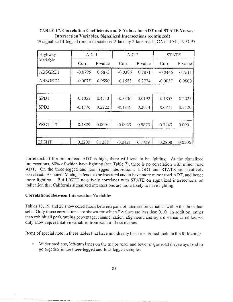
TABLE 17. Correlation Coefficients and P-Values for ADT assd STATE Versus
Intersection Variables, Signalized Intersections (continued)49 signalized 4-legged raral intersections, 2-lane by 2-lane roads, CA and Ml, 1993-9j
Highway ADT1 ADT2 STATEVariable
Corr. P-value Corr. P-value Corr. P-value
ABSG~l -0.0795 0.5873 -0.0396 0.7871 -0.0446 0.761 I
ABsGm2 ~ -0.0075 0,9590 I -0.1583 0.2774 I -0.0037 0.9800
SPD1 -0.1053 0.4713 -0.3336 0.0192 -0.18j3 0.2025
SPD2 -0.1776 0.2222 -0.1849 0.2034 -0.0871 0.5520
PROT_LTI 0.4829 0.0004 -0.0023 0.9875 -0.7943 0.0001
~LIGHT I 0.2200 0.1288 I -0.0421 0,7739 I -0.2808 0.0506 ~
correlated: if the minor road ~T is high, there will tend to be lighting. At the signalizedintersections, 80°A of which have lighting (see Table 7), there is no correlation with minor roadADT. On the three-legged and four-legged intersections, LIGHT and STATE are positivelycorrelated, As noted, Michigan tends to be less rural and to have more mirror road ADT, and hencemore lighting. But LIGHT negatively correlates with STATE on signalized intersections, anindication that California signalized intersections are more likely to have lighting.
Correlations Bet~veen I Intersection Variables
Tables 18, 19, and 20 show correlations between pairs of intersection variables within the three datasets. Only those correlations are shown for which P-values are less than 0.10. In addition, ratherthan exhibit all peak turning percentage, channelization, aligmnent, and sight distance variables, \vconly show representative variables from each of these classes,
Items of special note in these tables that have not already been mentioned include the following:
. Wider medians, left-turn lanes on the major road, and fewer major road driveways tend togo together in the three-legged and four-legged samples.
85

TABLE 18. Correlations Between Intersection Variables in the Tl]ree-Legged Sample
VARIABLE
ADTI
ADT2
EPKOhTRUCK
PK%TURN
SPDI
SPD2
HAZRAT
NODRWYI
MEDWIDTHI
FDEV
RSDI
Reciprocal Sight D]stance
HEI-I
Horizontal out to 800 ftB
l:::;:aloutto,ooft
j ABSGRDI
rLIGHTNo= O, YeS=l
1 ft = 0.305 m
POSITIVE COR~LATES N’EGATIVE CORRELATES
~
PK’?4TR UCK, PK%LEFT2
PKY,TURN, PKOALEFT, PKYoLEFTI, NODRW,YI.
ME DWIDTHI, HAU, SPDI ADTI, ADT2, NODRWYI, RSDI.
RS9R2, HEI-1, VI-), VEI-1, LIGHT1
ADT2, PKoALEFT, PKV,LEFTI , LTLN’2, RTLN2, PK<%THRUI
LIGHT
PKYoTRUCK, HAZRAT, LTLN 1, RTLN 1, ADT2, NODRWYI , RSDI, RSDR2,
MEDWIDTHI, SPD2 Hi-l, HEI-1, VI-I, VEI-1, VCEI-1,
LIGHT, STATE
HAZRAT, LTLN 1, RTLN 1, MEDWIDTH 1, ILIGHT, STATE
ABSGRDI. SPDi
LTLNl, HI-1, ABSGRDI, SPD1, SPD2 I NODRWYI, LIGHT, STATE
ADT2, RSDI, RSDR2, HI-1, HE]-], PK’XrRUCK, PiAZRAT, LTLN 1,
VEI- 1, LIGHT> STATE RTLNl, MEDWIDTH 1, SPDI
PKOATRUCK, LTLNI, RTLN 1, SPDI, SPD2 ,ADT2> NODRWYl, RSDl, Hi-l,
HEI-I. LIGHT
ADTI, HAZRAT, RTLNI, MEDWIDTHI, SPDI, NODRWYI, HI- I, HEI-I, VCI-1,
SPD2, STATE LIGHT
I>K% TRUCK, LIGHT, STATE RSDI, HI- I, ABSGRDI
RSDI, HEI-l I
::ABSGRD’’L”HT+ADTI, NODRWYI>DEV, HI-1, HEI-1, VI-I> PK”A,TR[JCK, MEDWIDTH 1, HAIJ,
NODRWYI, DEV, RSDI, RSDL2, RSDR2> FJI-1, PK”/.TRUCK> LTLN 1, MEDWIDTH 1,
ADTI, NODRWYI, RSDI, RSDR2, HI-1, IHEI-1,
1
PK”ATRUCK, SPDI
VI-I, VCI-1, vCEI-1, ABSGRDI
‘E1-’’VCESPD2SPD+IHAZRAT, RTLNI, RSDl, RSDR2, Hi-l, VI-1.
ADT2, PKOATURN, PK”ALEFT> NODRWY ILTLN2, HAU, RSD 1, STATE
86

VARIABLE POSITIVE CORRELATES NEGATIVE CORRELATES
E ‘K”A’EF’pKoAT;u2 -:
PK%THRUI, PK”ALEFT2, MEDWIDTH 1, SPDI PK”41’RUCK, PK%TLRN, PK”ALEFT,
PKYoTURN, PKY”LEFr, PK%LEFTI , PK”ATf{RU2, PI<%,. RLCI<, PI<’YoIIHRUI. HAZR.AT,
NODRWYI, RSDR2, HEI-1, LIGHT> STATE LTLNI, MEDWIDTHI, ,ABSGRDI, SPDI
ADT2, PK”ATURN, PK%L:FT, PKOALEFTl, PKY.’TRUCK, PKv”THRUI , FL4ZRAT,
CA= O, MI= I NODRWY1, HEI-1, VCI-1, VCEI-1, LIGHT LTLNl, RTLNI, MEDWIDTHI,
ABSGRDI> SPDI, SPD2—
PK%TRUCK PK0X1THRU2, LTLN 1, RTLN 1, RTLN2, SPD I ADTI, ADT2, PK%TURN, PK%LEFT,
PKYoLEFT1, HAZRAT, NODRWYI, DEV,RSDI, RSDL2, f<SDR2, LIG1+”I’, STA”rt.
—
PKUATURN ADT2, PKOALEFT, PK”ALEFTI, PK%rHRU2, ADTI, PKOATRUCK> PK”A,TIIRU 1, LTLS 1,NODRWY 1, LIGINT, STATE RrLhl i, RTLN2, VEDWIDTH 1, SPDI
SPD I ADTI , PK%TRUCK> PK%THRU 1. I..TLN 1, RTLN 1, ,\r)-r2. l~l<’’f)TLl{Y. Pl<!{,LEFT, f)I<’)<,l.EITl
RTLN2, MEDWIDTHI, SPD2 NODf?WYf. IRSDL2, RS[)R2. I-IEI-I. l.l GHT.yr~,f:
SPD2 LTLNI, RTLNI, DEV, SPDI NODRWYI, HEI-1, VI-1, VEf-1,\,Cl-l VCEI-I , STA”rE
—
HAZRAT LTLNI, DEV, RSDI , RSDL2, RSDR2, HI-I, ADT2, PK”ATRUCK, PK0ATHRU2, RTLN I >ABSGRDI RrLN2, STATE
—
40DRWY I ADT2, PK”ATURN, PK”ALEFT, PK”ALEFTI, RSDI PKOA;”rRUCK, PKY;I’HRU 1, l.”rLN 1, 1<’”1’l.?i1,
RSDL2, RSDR2, HEI-f, LIGH’r> STATE RrLN2, MEDWIDTH 1, SPDI SPD2—
AEDWIDTHI ADTI, PKY”THRUI, LTLNI, LTLN2, SPDI ADT2, PK%TURN, PK”ALEFT, PKOALEF:l,
NODl<\V}, 1, [.[clrr, STATE—
,TLN I PKOATRUCK, HAZRAT, RTLN 1, MEDWIDTH 1, ADT2, PK”ATU RN, PK”ALEFT, PKV”LEF71
SPDI, SPD2 NODRWY 1>VCI-1, VCEI-I , LIGtfT, STATE—
{AU DEV, ABSGRD I—
)EV HAZRAT, HAU, RSDR2, ABSGRDI, SPD2 PKY;rRUCK, RTLN 1, RTLN2—
(SD, RcciprOcal HAZRt\T, NODRWYf> RSDL2, KSDR2, HI-1, PK”4rRUCK, PK”XrHRU2, RTf,N I
;ight Distance ABSGRDI—
iE1-1, Horizontal out ADT2> NODRWYI, STATE SPDi, SPD2
0800 ft
{El- 1, Vertical out 10 RSDL2, VI-1, VCI-I vCEI-1, ABSGRDI f?’rLN2, SPD2
100 ft—
\BSGRDl HAZRAT, HAU, DEV, RSDI> RSDL2, RSDR2, FII-1, ADT2, PK”ATHRU2, RTLN 1, RTLN2,
VEI-I STATE—
.IGHT ADT2, PKVOTURN, PKOALEFT, PK”ALEFTI, PKOATRUCK, PK”ATINRUI, LTLN 1, RTLN 1,
NO=o, Yes=l NODf<WYl, STATE RTLN2, MEDwIDTH 1, SPDI
,.. —n?m. -
TABLE 19. Correlations Between Intersection Varizibles in the Four-Lezzed Sample
L ,, “.. ”., ‘,1
87

TABLE 20. Correlations Between Intersection Variahl in tl~e Signalized Sample
NEGATIVE CORRELATES
PKYoTURN, PKnALEFT, PK”A{rHRU2>
LT’LN2, STATE
PK%THRUI, SPDI
—
POSITIVE CORRELATESVARI~LE
ADT1 PKOATHRUl , RSD 1, RSDLI , RSD2, pROT_LT
ADT2 Pi<”ATURN, PK”ALEFT, PK%LEFTI >NODRWY I>
RTLN2, HEI-l , HEICOM, STATE
ADr2, PKYoTURN> PKVOLEFT, NODRWY I Al)Tl, HAL R.AT, I.’rLNl.ME; DWIDTIII, HI-2, 111:1-2
PROT LT, LIGHT
STATE
CA= O, MI= I
SPD2
ADT2, PKYoLEFT, PK%LEFTI, NODRWYI, HE]-),HEICOM, VEI-1, VEICOM, VCI-2, VCEI-2,
VCEICOM, ABSGRDI
PKVOTRUCK
AOT2, PK%THRUI PI<UATHRU2,
SPD I
PK%TURN
—RTLN 1, RTLN2, SPD2 ADT2, PKYoTURN, PK”ALEFT,
NODRWYI, NODRWY2, RSDI,
RSDLI, RSDL2, HEI-1, t{ EICOMVCEI-1, LIGHT
SPDI
Pi<%TRUCK, PK0ATHRU2, LTLN 1, RTLN2, SPD I PK:%LEFT2, NODRWYI,
NODRWY2, RSDI RSDLI, RSD2.
RSDL2 HEICOM, LIGHT
SPD2
RSDI, VCE1-I
ADT2> PKYoTURN, PK”ALEFT, NODRWY2, RS132>
RSDL2, STATE
PK%LEFT2, NODRWYI, RSDL2, LIG}[T
VI-2, vEI-2, VCI-2, VCE1-2, VCICOM, VCEICOM.PROT LT
NODRWY2, RTLN 1. VCI-I , STATE{AZRA7
PK”ArHRUl, Hi-2, PROT_LT, SPDI>
SPD2
PK”ATHRU2, HAZRAT, SPOI , SPD2
40 DRWY1
40 DRWY2
RTLN2, HAU, STATEJEDWIDTHI
HEI-I , VCI-I STATE
HI-I. HICO,M
.TLN I
+AU
LTLN2, PROT,_LT, SPD2
MEDWIDTHI
HI-I, HICOM
ADTI, HAZRAT, RSDLI , RSD2> RSDL2, HI-1,
HEI-1, tlEICOM, VI-1, VEI-1, VCEI-1, ABSGRDI,
PROT_LT, VEI-1, ABSGRDI, LIGHT
ADTI, PK%LEFT2, NODRWYI, RSDI, RSDLI, Hi-2
HE[-2, ABSGRDI, ABSGRD2
ADT2>PKVOTURN, PKOALEFT, PK0ALEFTl, RSDI,
RSDL2> HI- I, HI-2, HICOM, HE1-I, HE1-2, VEI-1,vCE1-I, ABSGRDI
PK’%TURN> VI-I. VI-2, VICOM, VET-I> VE1-2, VCI-I
VCI-2, VCICOM, VCEI-1> VCE1-2, VCEICOM,ABSGRDI> ABSGRD2
—
)EV
R’LN 1, SPDI> SPD2<SD 1, Reciprocal
jight Distance
along Maior Rw.d
PK%THRU2, SPD2
PKO/”Tl-{RUI , SPDI, SPD2
<SD2, Recip. Sight
~ist alonz Minor Rd
HEICOM
Horizontal out to
300ft, All legs
VEICOM, Vctiical f>lKOA,THR U
out to Soo ft,
All legs
ft = 0.305 m
88

TABLE 20. Correlations Between Intersection Variables in the Signalized SampIe(continued]
VARI~LE POSITIVE CORRELATES NEGATIVE CORRELATES
ABSGRD1 PK%TURN, PKV.LEFr> PK.V,T1+RUI, MEDWIDTH I
Major Road RSD1, RSD2, RSDL2, HI-1 >HICOM, V:-1 , VICOM,VEI-1, VEICOM, VCI-1>VCEI-1, VCEICOM,ABSGRD2
&BsGm2 RSD2, VI-2, VICOM> VEI-2,Minor Road VEICOM, VCI-2, VCICC~M,
VCEI-2, VCEICOM,ABSGRDI
LIGHT PK%LEFT2, NODRWY2> PKVOLEFTI, RTLN2> SPDI,
~o=O, Yes=l RSDLI , RSDL2 SPD2, STATE
?ROT_LT ADTI, LTLN1, NODRWYI , STATEiO=O, Yes=l MEDWIDTH1 , RSD 1,
RSDL1 , HEI-2
o Major road speeds tend to be higher when major road channeiization is present and whenmedims are wider in the three-legged and four-legged samples.
o Major road speeds tend to be lower when minor road ADT is higher, when there are moremajor mad driveways, when sight distance is restricted, when lighting is present, or whenhorizontal or vertical curves are present. This happens in all three data sets.
o Lighting is more likely to be present when minor road ADT is high, when the peak turning;percentages are high, or when the number of major road driveways is high. This applies tc,the three-legged and four-legged samples.
o At signalized intersections, protected lefi turns are more likely to occur in California than inMichigan (17 out of 18 CA signalized intersections have pro!ected left turns, while only ~1out of31 MI signalized intersections do).
A couple of anomalies are evident from the tables. In Table 19, for the four-legged intersections,a negative correlation exists between the presence of a left-turn lane on the m~ or road and peakturning percentages, including major road left turns. When a higher fraction of the traffic is turning,it is less likely that there is a turning lane. It may be that the motive for installing turning lanes ismore to prevent disruption of through traffic than to assist turning drivers. Another oddity, this tiln,s
89
in Table 20 for signalized intersections, is the negative correlation between HAZRAT and VC1- 1,accompanied by a positive correlation between HAZRAT and VCE1- 1. HAZRAT is measul-ed out.to 250 feet (76 meters) as is VCI- 1, while VCEI- I is measured out to 800 feet (244 meters). A totalof 37 out of 49 signalized intersections have VCI equal to zero, while 25 out of 49 have VCEI equalto zero. The two highest hazard ratings occur at intersections with VC1 equal to zero, but with VCE1.
equal to 6.0 and 3.46 (average VCEI is 0.952), and this contributes to the anomalous correlation.
Correlations for Single-Vehicle and Multiple-Vehicle Crashes at Signalized Intersections
For the si~alized intersections, an attempt was made to analyze single-vehicle crashes and multiple-vehicle crashes separately and to relate them to various flow patterns deli \c(i from [be traffic data.The variables TOTACCS and TOTACCM, representing a decomposition of TOTACC into sinSle-vehicle crashes and multiple-vehicle crashes, were compared with the intersection variables and with.the flow variables Fl, Fz, F,, F~, PRODFADJ, PRODFOPP, ar~dSUMF. The correlation coefficientsand P-values are shown in Table 21.
Conclusions that can be drawn from Table21 with regards to the signalized sample arc:
4 Single-vehicle crashes show a slight negative correlation with major road ADT and majorroad flows.
o Multiple-vehicle crashes are strongly correlated with minor mad flows and with theinteraction variable for adj scent legs, as well as with peak truck percentage and left-turnpercentage on the major road.
. HAZRAT’S correlation coefficient has the correct sign for single-vehicle crashes, but isinsignificant, as are the driveway variables.
. Horizontal alignment variables are negatively correlated with both kinds of crashes (one mayspeculate that horizontal alignment causes drivers to exert ex!ra caution at signalizedintersections), and protected left turns reduce both kinds of c!-ashes.
* Minor road vertical alignment contributes to single-vehicle crashes, and lighting reduce!jthese crashes significantly.
The correlation of both kinds of crashes with the STATE variable has already been noted, i.e.,Michigan is overrepresented in crashes. However, since STATE has a strong negative correlationwith PROT_LT, it is not clear which of these two vaIiables has the dominant influence.
Turning Percentage Variables
Intersection crashes are naturaliy related to turning percentages at illterSCC[iOnS. However. sorting
out the relative importance of left turns versus right turns and turns from the major road versus the
90

TABLE 21. Correlation Coefficients and P-Values for Single-Vehicle and Nlultipie-Vehicle
49 sCrashes Versus Signalized Intersection Variables
a]i7ed 4-Ie~ued rllral intersections. 2-lane bv 2-lane rn~~~ CA ~nd Ml. 1‘------ ,.==-— .. ---., --- ---—- -.,
Highway TOTACCS TOTACCM
VariableCorr. P-value COrr. P-vall[e
ADTI -0.1175 0.4213 0.0386 0.7923
ADT2 0.1682 0.2480 0.4545 0.0010
F, -0.1140 0.4365 0.0303 0.8365
F, -0.0722 0.6222 0.0809 0.5807
F, 0.1650 0.2571 0.3048 0.0332
F, 0.0584 0.6904 0.4461 0.0013
PRODFADJ 0.1018 0.4865 0.3931 0.0052
PRODFOPP -0.0588 0.6882 0.1543 0.2899
SUMF -0.0201 0.8907 0.2349 0.1043
‘KO/OTRUCK 0.1853 0.2025 0.2558 0.0761
‘KO/OTURN 0.1132 0.4386 0.2075 0.1526
‘KO/OLEFT 0.1188 0.4161 0.2136 0.1406
‘KO/OTHRUl -0.0793 0.5882 -0.2’763 0.0546
‘KO/OLEFT1 0.1450 0.3203 0.3579 0.0116
JK0ATHRu2 -0.0374 0.7986 0.1664 0,2533
‘KO/0LEFT2 -0.1490 0.3069 -0.3220 0.0240
IAZRAT1
0.1001 0.4938 -0.0030 0.9838
~G:: ~~

TABLE 21. Correlation Coefficients and P-Values for Single-Velhicle and.Mu1tiple-VehicleCrashes Versus Signalized Intersection Variables [continued)
49signalized 4.1egged mralintersections, 2-lane by2-lane roads, CAand MI, 1993-95
High}vayVariable
LTLN1
RTLN 1
LTLN2
TOTACCS I TOTACCM 1
0.0683 0.6410
-0.0727 0.6194
-0.1314 0.368;
-0.1764 0.225:
RTLN21
0.2169 0.1345 0.2232 0.1231
MED WIDT1-11 -0.0724 0.6209 -0.0297 0.8395
HAU -0.0737 0.6149 0.0054 0.9704
DEV -0.0708 0.6289 -0.0508 0.7288
RSD 1 -0.1429 0.3275 -0.0965 0.5095
RSDLI -0.1760 0.2265
RSD2 -0.1453 0,3191
-0.1938 0.1821
0.0341 0.815s
RSDL2I
-0.2095 0.148j -0.0293 0.8415
HI- 1
HE1-1
HI-2
HE1-2
HICOM
HEICOM
-0.1041 0.4766
-0.1815 0.2121
-0.1812 0.2128
-0.1750 0.2292
-0.1924 0.1853
-0.2382 0.0993
0.01j6 0.91j0 ~I
-0.2258 0.11871
-0.1577 0.2792
-0.3184 0.0258
-0.040 I 0.7529
92

TABLE 21. Correlation Coefficients and P-Values for Single-Vehicle and MuItiple-VehicleCrashes Versus Signalized Intersection Variables (continued)
49 signalized 4-legged rural intersections, 2-lane by 2-lane roads, CA and Ml, 1993-95
Highway TOTACCS T(lTACCklVariable
Corr. P-value Corr. P-value
VI- 1 -0.0295 o.&403 0.073j 0.6156
VEI- 1 -0.0421 0.7741 0.2442 0.0908
VCI- 1 -0.0302 0.8367 0.2148 0.1384
VCEI-I -0.1738 0.2324 0.0808 0.5811
VI-2 0.3434 0.0157 0.0856 0.5587
VEI-2 0.3269 0.0219 0.1026 0.4829
VCI-2 0.3238 0.0232 0.0578 0.6934
VCEI-2 0.3051 0.0331 0.1050 0.4729
VICOM 0.2749 0.0559 0.1043 0.4759
VEICOM 0.2629 0.0680 0.1895 0.1922
VCICOM 0.2818 0.0498 0.1264 0.3867 ~
VCEICOM 0.1924 0.1853 0.1315 0.3680
ABSGRD 1 -0.0753 0.6071 0.0487 0.7398 I
msGRD2 0.1030 0.4812
9
SPD 1 0.0794 0.587j
SPD2 0.1588 0.2758 a
PROT-LT I -0.3996 0.0045 -0.2449 0.0899
LIGHT 1 -0.4359 0.0017 -0.0672 0.6464
~ ISTATE 1 0.3356 0.0184 ] 0.3387 0.0173
93

minor road, as well as the direction of the effect in each case, is not easy since the turning percentagevariables are strongly related to one another. In Tables 22 and 23, some of the relevant correlationcoefficients are presented.
Table 22 shows the correlation coefficients for the various turning percentages. It supports the con-
ventional wisdom, although not perfectly. PKOALEFT1 correlates positively with PKO/0RIGHT2
TABLE 22. Correlation Coefficients and P-Values for Peak Turning Percentage Variables
Variable Pair 3-legged 4-legged signalizedCorr. P-value COrr. P-value Corr. P-valL1c
PK%LEFT 1Vs. PKYoTHRU1 -0.8853 0.0001 -0.8964 0.0001 -0.7744 0.0001
PKYoRIGHT1 0.5588 0.0001 0.6519 0.0001 0.2101 0.1473
PKYOLEFT2 -0.2891 0.0084 -0.1704 0.1584 -0.4724 0.0006
PK%THRU2 0.2642 0.0271 ().1307 0.3709
PK%MGHT2 0.2891 0.0084 -0.0109 0.9290 0.3477 0.0144
‘KO/OTHRUl1s. PKYoRIGHT1 -0.8803 0.0001 -0.9205 0.0001 -0.7813 0.0001
PKVOLEFT2 0.0165 0.8829 0.02418 0.8385 0.0716 0.6248
PKYOTHRU2 -0.29:!7 0.0136 -0.0995 0.4965
PK%MGHT2 -0,0165 0.8829 0.1621 0.1801 0.0491 0.7378
?KO/ORIGHT17s PKYOLEFT2 0.2673 0.01j2 0.1077 0.3750 0.3554 0.0122
PKYOTHRU2 0.2686 0.0245 0.0248 0.8657
PKYORIGHT2 -0.2673 0.0152 -0.2670 0.0255 -0.4189 0.0027
?KO/0LEFT20s. PK%THRU2 -0.1966 0.1028 -0.6536 0.0001
PK%RIGHT2 -1.0000 0.0001 -0.78’74 0.0001 -0.2543 0.0779
PKYOTHRU2vs. PK%MGHT2 -0.44?5 0.0001 -0.5657 0.0001
94

(exception: the four-legged intersections where the correlation is negligible) and negatively w~thPKYoLEFT2. Likewise, PKOARfGHTl correlates positively with PKY.LEFT2 and negatively withPK0ARIGHT2. The positive correlations are expected since the corresponding flows are !revetsalsof one another, The negative correlations result at least in part from the fact that pKO/0LEFT2 and
PK0ARIGHT2 are negatively correlated with one another. The four- lc~:ed intel-sections at-e lessregular than the other two intersection classes. These correlations al-e, of course, based on roughinformation since peak hours in the morning and the afternoon were selected in a crude manner andthere is no reason why flows should reverse in any precise way (even if peak hours were selectedwith great care).
Table 23, extracted in part from Tables 11, 12, and 13, shows the relationship between the crashvariables and the turning percentages for the three classes ofintersectiolls. What immediately strikesthe eye is that PKYoLEFT 1 is positively correlated with all types of crashes at all types ofintersections, while PK0ALEFT2 (or for that matter PKO/OTHRU1) is negatively correlated with alltypes of crashes at all types of intersections. Since PK%LEFT2 = 100 PK%THRU2PK%RIGHT2, what is being said is that the sum of PKV.TI+RU2 and PKY0RIGHT2 is positivelycorrelated with crashes. The last two columns of Table 23 confirm this. In general, bothPKV”THRU2 and PKY0WGHT2 are positively correlated with crashes; in cases where one of them
TABLE 23. Correlation Coefficients and P-Values for Crashes Versus Peak TurningPercentage Variables
PKVOLEFTI PK%THRUI PKoARIGHTl PK(Y, L,EFT2 PK’Y,TIIRU2
TOTACC
3-legged 0.2786,0.0103 -0.2170,0.0474 0.1027,0.3525 -().2()96, 0.0j8S4-legged 0.3532,0.0023 -0.3022,0.0099 0.205j, 0.0833 -0.1021.0.4003 t).1688,0.162jsi~nalizcd 0.3557,0.0121 -0.2693,0.0614 0.0652, ().656j -0.3230,0.0236 0 14S2, 0.309G
TOTACCI
3-legged 0.3098,0.0041 -0.2819, 0.0094 0.18G7> 0.0890 -0.19 C’O,().0873
4-lcZged 0.3794,0.0010 .0.3263 ,0.0052 0.2235,0.0590 -0.10 ss,0.3702 0.2013,0.0948signalized 0.3507, 0.0)35 -0.2472, O.OSGS 0,03 Gl,0.80jG -().3G29, [).0104 O.199G, O.l G92
INJACC
3-legged 0.2612,0 .01G4 -0.1745,0.1123 0.0448, 0.6SGI -0,162,8 >0.1440
4-legged 0.2020>0.0889 -0.1457, 0.2219 0.07) 2>0.5521 -0,0883>0,4674 0,08[3, 0.5033signalized 0.1521,0.2967 -0. OGGO,0.G524 -0.04 S)>0.7427 -0.252.G> 0.0800 0.1176,0.4210
[N JACCIl-legged o,28S4, o,o07S .0,2242 ,0.0403 0. I05G, ().3389 -(1. 144G, 0.1950!-legged 0.2190, 0.0G45 -0. IG47,0. IGGS 0.0S8G, 0.4j91 ,-o.09GI. 0.4288 0.10 S),0.3729;ig”alized 0.1450>0.3203 -0.00sG, 0.9533 -0,1298,0.3742 -0.3101, 0.030) 0.1686, 0.2468
TOTACCS;ignalized 0.1450,0.3203 -0.0793,0.5882
L
.O.020j, ().S887 -O. !490, 0.3069 -0.0374, 0.798G
TOTACCM
signalized 0.3j79, 0.0116 -0.2763, 0.054G 0,07j9,0.G 14(1 -().32:20, ().()24()
[).2096, (1.oj88O,oljl, (1.9144
[).1626, 0.2643 I
d0.1900, 0.0s73
0.0275>0.82150.[403, 0.33G2
40. IG28, 0.14400.0293, ().80980.1249, 0.3925
d‘1.)446, 0.)950
).019G, [).8723).1224. (1.4022
+
),2[01 ,0.1473
,).13s 3, (1.34.34
95

is not (and in those cases, the correlation is insignificant), the other one is still positively correlatedwith crashes. Right turns horn the minor road, including right turns on red, are certainly occasionsfor crashes. It might be argued that drivers turning left from the minor road are more vigi Iant thandrivers turning right md are at less risk than drivers going through (between legs 3 and 4). Driversturning left from the major road, at least at the three-legged and four-legged intersections, nlust beconcerned about both opposing traffic and traffic behind them, whereas drivers turning left from astop-controlled minor road have less risk from traffic behind them. According tO Table 22,PKVOLEFT2 correlates negatively with PKVOLEFT1. This suggests that the negative correlation O:f
crashes with PKO/0LEFT2 may, in part, be a consequence of the positive correlation of crashes withPK%LEFT1.
Crashes Versus ADT
Examination of correlation coefficients shows that ADT unsupported by other variables, especiallyADT1, plays a smaller role as one passes from three-legged to four-legged to signalizedintersections. To understand this phenomenon better, we examine grouped data in the InanncrofHaueretal. (1988). Foreach of thetkee data sets, intersections were divided into four groups byincreasing major road ADT with an effort to equalize thenumberofcrashes in each group to theextent possible. Likewise, intersections were divided into four grotlpsby increasing minor roaclADTwith roughly equal crash counts in each group. Then, 16cells were defined bymeansoftllcgrouping. Ineachcell, thenmber ofintersections wascourlted, alongwith thenumberofcrashe~(TOTACC) at its intersections during 1993-1995 and the ratio (the a~erage number of crashes perintersection). The numbers obtained are shown in Tables 24, 25, and 26. In addition, Imarginalcounts were made for the major road ADT groups and the minor road ADT groups of the samevariables (number of intersections, number of crashes, and average number of crashes perintersection).
Itisevident &omthetables thatsome cells wereempty orsparsely occupied. Forexample, in Table24, there are no intersections in the highest quartile for major road ADT and the second highestquartile forminorroad ADT. There arealso twoempty cells in Table 25. Ifthecells were unifonlllyoccupied, theaverage number ineacll cell would be84/l6=5.2j, 72116 =4.5, and 49/16 = 3.1 inTables 24,25, and 26, respectively.
[n Figures 5, 7, and 9, the marginal distributions with respect. to major road ADT am plotted, and mFiWres6, 8,mdl O,tllose with respect tominor road ADT are plotted. Thehorizontal variableirleach case is the median ADT of the group, and the vertical variable is the average number of crashe!;perintersection inthegmup, Thenumber ofcrashes perintersection generally appears to]ncreasl:with increasing minor road ADT, with allowances made for noise due to the smallness of the samplesizes. The number of crashes per intersection versus major road ADT shows a similar but momerratic trend, except fortlle signalized intersections (Figure 9). The plot for the Iatter shows ver:!little change inthecrashes perintersection asmajor road ADTisval-ied. Note the scale.
96

TABLE 24. Crashes Versus Grouped Major and Minor Road ADT, Three-Legged Sample3-legged, 4-lane by 2-Iane, stOp-controlled mral intersections, CA ~_~95
hro. of IntersectlollsAD T 1
NO. of Cl-ashesCrasheslIntersection 2,367to ll,917to 15,168 to 17,379 to
11,916 15>167 17,378 33,058~~ ~
A 15-250 22 5 2 6 :5
18 21 , 7 33 79
0.82 4,20 3.50 5.jO 2.26
D251-820 11 6 1 7 2j
30 20 6 31 872.73 3,33 6.00 4.43 3.48
T821-1>270 6 4 3 0 13
23 19 33 7j3.83 4.75 11.00 j.77
1,271-3,001 2 4 2 3 119 29 23 24 8j4.50 7.25 11.50 8.00 7.73
*
41 19 8 16
n
8480 89 69 88 326
1.95 4.68 8.63 5.50 3.88
3-Legged, 4-Lane by 2-Lane, Stop-Controlled Rural intersections
10
~..
o
CA&Ml, 1993-95
❑
❑
. . .....=
5000 10000 75000Grouped Major Road ADT
,.
20000 25000
FIGURE 5. Crashe5 Versus Major Road ADT, Three-I, egged Sample
97
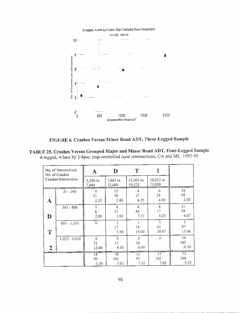
3-Legged,4-Laneby2-Lane,Stop-ControlledRura Intersecltons,
CA8MI, 1993.95
E
m
m’
500 1000 1500 2000GroupedMinorRoadADT
FIGUW 6. Crashes Versus Minor Road AD~, Three-Legged Sample
TABLE 25. Crashes Versus Grouped Major and Mino}r Road ADT, Four-Legged Sample4-legged, 4-lane by2-lane, stop-controlled rural intersections, CAand MI, 1993-95
$0.of lntersectiOtls{o. of Crashes;rasheslIntersectiOn
A
+341-800
D k801-1.051
T
P
AD T, II
3,350 to 7,685 to 12,001to
7,684 12,000 19,332 I:%0iL
mEI 17 I 18 I 62 II 97
5.56 18.00 20.67 13.86
6 2 2 0
r
1072 17 16 10512.00 8.50 8.00 I0,5C
1 1
18 28 13 13
m
7299 101 95 103 398
5.jO 3.61 7.31 1.92 5.53
98

4-Legged, 4-Lane by 2-Lane, Stop-Controlled Rural Intersections,
0:...... .. .0 5000
CA & Ml, 1993-95
-..
10000 15000 20000Grouped Major Road ADi’
25000 30000
FIGUW 7. Crashes Versus Major Road ADT, Four-Legged Sample
4-Legged, 4-Lane by 2-Lane, Stop-Controlled Rural Intersections,
CA & Ml, 1993.95
15 ~~~~~~~~~m
oo 200 400 600 800 1000 1200 1400 1600
Grouped Minor Road ART
FIGU~ 8. Crashes Versus Minor Road ADT, Four-Legged Sample
99

TABLE 26. Crashes Versus Grouped Major and Min{)r Road ,~DT, Signalized SampleSignalized, 2-lane by 2-lane, 4-legged rural interse(:tions, C.A and, MI, 1993-9:
No. of Inters ectlOus
NO. of CrashesA D T 1
Crashes/Intersection 4,647 to 7,581ta 8,834 to 12,826to7,580 8,833 12,825 25,133
H- ~~ i
A 940-3,003 4 3 1 7 1570 65 17 98 2j017.50 21.67 17.’30 14.00 16.67
D3,004-4,192 4 3 4 2 13
68 69 119 13 26917.00 23.00 29.75 6.50 20.69
T4,193-5,450 4 4 4 1 13
76 78 79 25 25819.00 19.50 19.75 25.00 19.85
1 1 3 3 8
+, * ;: :: *I &l
Signalized, 2-Lane by2-Lane, 4-Legged Rur:sllntersections,
CA8 MI, 7993-95*S... ,..
o0 5000 i 0000 15000 20000
Grouped Major Road ADT
FIGUW 9. Crashes Versus Major Road A.DT, Signalized Sample
100

Signalized, Z-1ane by 2-Lane, 4-Legged Rural Intersections,
CA&Ml, 1993-9535 .. .. ..
2 ~ .-,
~ ,..
0 2000 4000 6000 8000 10000Grouped Minor Road ADT
FIGUW 10. Crashes Versus Minor Road #,DT, Sigl~alized Sample
A.M. Versus P.M. Truck Percentages
Thelarge amount oftraffic movement data collected forthis repofi permits avarietyofspccialstudies. Table 27isone illustrative example. Forreiated items, seethe appendix.
Table 27indicates thattie tickpercentage issomewhat vaiable, mdthatin themoming, thetmckpercentage ishi@er thanintie evening (except forthe Michigan sigIlalized intersections). Miaouet al. (1993) recommend that future studies include a time-of-day variable in estimating truckpercentages.
CONCLUSIONS
This chapter began with the development of variables for malysis and modeling. A variety ofvariables were constructed relating to crash counts, ADT, peak-hoar truck traffic, tumin:~percentages, geometry, channelization, alignments, and driveway counts. A variable for State was
defined, underscoring the possibility that in different regior~s andjor epochs, crash experience maybe quantitatively distinct despite similar values for intersection variables.
101

TABLE 27. A.M. and P.M. Truck Percentages by State
3-Legged Intersections
California (60) Michigan (24) CA& Ml (84)
W%TRUCK 10.11 10.31 10.17
PMVOTRUCK 9,19 6,$18 8.56
PK%TRUCK 9.52 8.21 9.15
4-Legged Intersections
California (54) Michigan (18) CA& MI (72)
AM%TRUCK 13.76 8,94 12.56
PM%TRUCK 10.98 7.11 10.01
PK%TRUCK 11.98 7.83 10.95
Signalized Intersections
California (18) Michigan (31) CA& MI (49)
AMY”TRUCK 8.34 9.70 9.20
PMYoTRUCK 6.62 10.16 8.86
PKYoTRUCK 7.36 9.89 8.96
Then. in Tables 5, 6, and 7, a summaW of univariate statistics for these variables on the three datasets was given. More crashes occur at si~alized intersectior~s than at fore-legged intersections, antimore occur at four-legged than at three-legged intersections (cf. Table 8). Crashes tend tO be mOresevere in California (Table 9), but more frequent in Michigan (Table 10). While this may, in part,be attributable to systematic differences in intersection variables between the two States (cf. Tables15, 16, and 17), it is a reminder that the STATE variable may make an independent contribution.
The chapter also examines correlations between pairs of variables. This includes cmshcs \e!-su!s
other variables (Tables 11, 12, 13, and 14), ADT and STA.TE versus other intersection variables(Tables 15, 16, and 17), single-vehicle and multiple-vehicle crashes versus other signalizedintersection variables (Table 21), and turning percentage variables (Tables 22 and 23). The moststriking finding is the relevant insignificance Of major road ADT in relation to the signalizef~intersection crashes (see especially Figure 9). Another finding of impoflance is the negativ,acorrelation between minor mad left-turn percentage and crashes present for all three intersectionclasses (Table 23). This, of course, implies a positive correlation between crashes and the sum of
102
minor road through and right-turn percentages. Given the range of minor mad left-turn percentageswithin and among the three data sets (Tables j, 6, and 7), this seems especially significant. Sincethe hazards that a left-turning vehicle faces are greater than those that a right-turning vehicle faces,the possibility exists that driven m~ing Iefi turns from the mirror road exercise more care than other
drivers approaching the intersection from a minor leg Perhaps more relevant is the fact that sincelefi-turn percentages from the minor road correlate negatively with right-turn percentages from theminor road, they also correlate negatively with Iefi-tum percentages from the major road. As minorroad left turns increase, major road left turns decrease, and the net effect of the two opposi[e changesis to reduce crashes.
An issue that will affect the modeling is the multival-iate relationships, especially the relationshipamong crashes and pairs of highway variables. Thus, for the signalized intersections, the relativeinsignificance of crashes versus major road ADT may indicate the effect of a third variable thatcorrelates with ADT. Again, for the signalized data, the effect of STATE on crash counts may beconfounded with that of other variables such as LIGHT, PROT_LT, HAZWT, NODR WY 1,MEDWfDTHl, and even ~Tl, all of which strongly correlate with STATE. The general strategywill be to see which vwiable has the chief effect, in accordance with common sense, and, thereafter,to determine which remaining variable, if any, has a significant effect on the residual, ie., the poflionof the crash count not predicted by the chief variable.
103

5. MODELING
In this chapter, we use the sample data to develop generalized line~ models Of the poisso~negativebinomial type for the mearr number of crashes per unit time at an intersection in terms of theintersection variables discussed in earher chapters. These mcldels summarize the data collected. Itis hoped that they have predictive value for other data sets from the same intersection classes.
The chapter begins with a review of some of the theoretical aspects of model bui Iding andmeasurement of goodness of fit. Thereafter, models are built for each of the three classes ofintersections. This is done for each of the four crash variables — TOTACC, TOTACCI, INJ ACC,and NJACCI. We study how these variables can be represented in terms of maj or and minor roadDT, md then we add variables with the aim of improving the fit and discovering design elementsthat might affect safety.
Separate models are also developed for TOTACCS and TOTACCM in the case of the signalizedintersections. These models use only the flows F,, FZ, F3, and F~ as explanatov vari ab~es.
Finally, the main models for TOTACCI are subjected to residual analysis to uncoier systematicshortcomings.
THEORY
Modeling
We shall use a negative binomial model with mean a generalized linear function of intersectionvariables. Thus,
(5.1)
where vi is the mem number of crashes to be expected at intersection number i in a given time
period; xi,, .... x;~, are the values of the intersection variables at this intersection during that timeperiod (xi, = 1 corresponds to the intercept term); and ~,, ... ~p are coefficients to be estimated bythe modeling. More sensitively, one might say that pi is the grand mean of crashes to be expectedat a hypothetical population of intersections having the same values as intersection number i for theintersection variables considered. Variables not included in the model account for differences in theexpected number of crashes among members of this population, and these differences are describec,by the term overdlspersion. See lIauer et al. (1988). The variance (oi)2 of the number of crashes inthis population under the model is:
105

(oi)’ = pi + K(p,)2
where K is the overdispersion parameter. The second tem on the right side of this equationrepresents the variation in means among different members of the population existing even when allintersections have the same value for the considered intersection variables. In principle, K could alsodepend on these intersection variables, but for simplicity, that possibility is ignored.
Under the negative binomial model, the probability of yi cmshes at intersection number i is givenby:
men K equals O, the negative binomial reduces to the Poisson model. The larger the value of K,the more variability there is in the data over and above that associated with the mean )i
The coefficients ~j are estimated by maximizing the log-likelihood function L(P, K) for the negdtivebinomial distribution. The likelihood function is the probability that the values y,, .... y~ would be
observed for intersections number 1 though N. If crash counts are independent at the differenl:intersections, the likelihood is:
and application of the logarithm yields the log-likelihood function:
(5.2)
Here, p = (@l,..... ~P) is the vector of coefficients, yi is now taken to be the observed crash cOLmta.t
intersection no. i, and Yi is given by equation (5.1). The values of ~ and K that maximize the
106

function L(P, K) in (5.2) are the estimated coefficient vector ~ and ti~c estimated ovel-dispersionparameter K The estimated value of )i obtained by substituting ~ and ~ for ~ and K i~lequation(5.1) is denoted by Y,. For convenience, tbe same letters will often bc LISedfor both the pammeters
and their estimated values, i.e., carets ~) will be omitted in references to ~ and ~.
P-Values and Goodness of Fit
The modeIing of the data in this study was done using SAS and LIIM”DEPsoftware. Along withapproximate maximum likelihood estimates for the regression coefficients, these software packagesyield estimates of the standard error for each coefficient. From these, P-values can be computed forthe null hypothesis that the tme value of some regression coefficient is zero. The z-score of theestimated coefficient is the estimated coefficient minus zero, divided by the estimated standard error.The P-value is the probability that a norrnaI random variable has an absolute w~iue larger than thez-score obtained. If dre P-value is small, we have good evidence that t~te corresponding variable issiamificant, that the difference between the coefficient estimate and zero arises not from chance, butfrom a systematic effect. Even if tie P-value is large, the parametel- estimate has some value sincethe null hypothesis that the parameter is zero is a somewhat arbitrary starting point and the estimateobtained is the one dictated by the data. A large P-value lowers our confidence in the estimate andindicates that even if the basic model form is correct, the true coefficient may be quite different fromthe one estimated. One may expect the true coefficient to be within one or two estimated standarderrors of the estimated coefficient.
Goodness-of-fit measures associated with Poisson-type models have been introduced and reviewedby Fridstram et al. (1995) and Miaou (1996). For the modeling, we shall use three measures ofgoodness-of-fit.
One measure is the ordinary R-squared, or coefficient of determination, used in linear regressionmodels:
where
Yi = observed crash count for intersection no. i,
—
Y = average crash count for the sample, and
(j.3)
91 = estimated mean crash count for intersection no. i.
107

This measure is used because of its great familiarity. In case a model with no variables is used, i.e.,in equation (5.1), Vi = exp(~o) so that there is only a constant or intercept term in the iinearexpression, the maximum likelihood estimate for Docan he shown to yield
and hence, R2 equals zeroprinciple, happen that
~?i E j
This model is called the zero model. At tbe other extreme, it might, in
yi = yi
for each i, and hence, R2 equals 1. The value of R* is alway> less tha]l or equal to 1 hy definition.
It is greater tha or equal to zero since maximum likelihood guarantees a result at least as good asthe zero model.
FridstrOm et al. (1995) have pointed out that in Poisson or negative binomial models, R2 is veryunlikely to equal 1 since a Poisson-type variable takes a variety of values other than its mean, andyl is unlikely to equal the estimated mean $i for each i in a sample of any appreciable size. Theyhave proposed taking a ratio of R* to its largest expected value P2 under a best fit as a measure ofgoodness-of-fit.
A form ofthLs that they recommend for negative binomial models is tile lag-likelihood R-squared,based on the deviance V of the model. The deviance ofa model m is:
where
is the log-likelihood that would be achieved if the model did give a perfect fit (vi= yi for each i, and
K = O). Such a model is called the full or saturated model by FridstrOm et al. V is the log-Iikelihood, as in (5.2), of the model under consideration (/Li= ~i). If the latter model is correct, D“’is approximately a chi-squared rdndom variable with degrees of freedom equal to the number N o fobservations minus the number of parameters. The number of parameters is (p + 1), where p is th{:number of explanatory variables in the model plus the intercept, and the extra 1 is for theoverdispersion parameter.
108
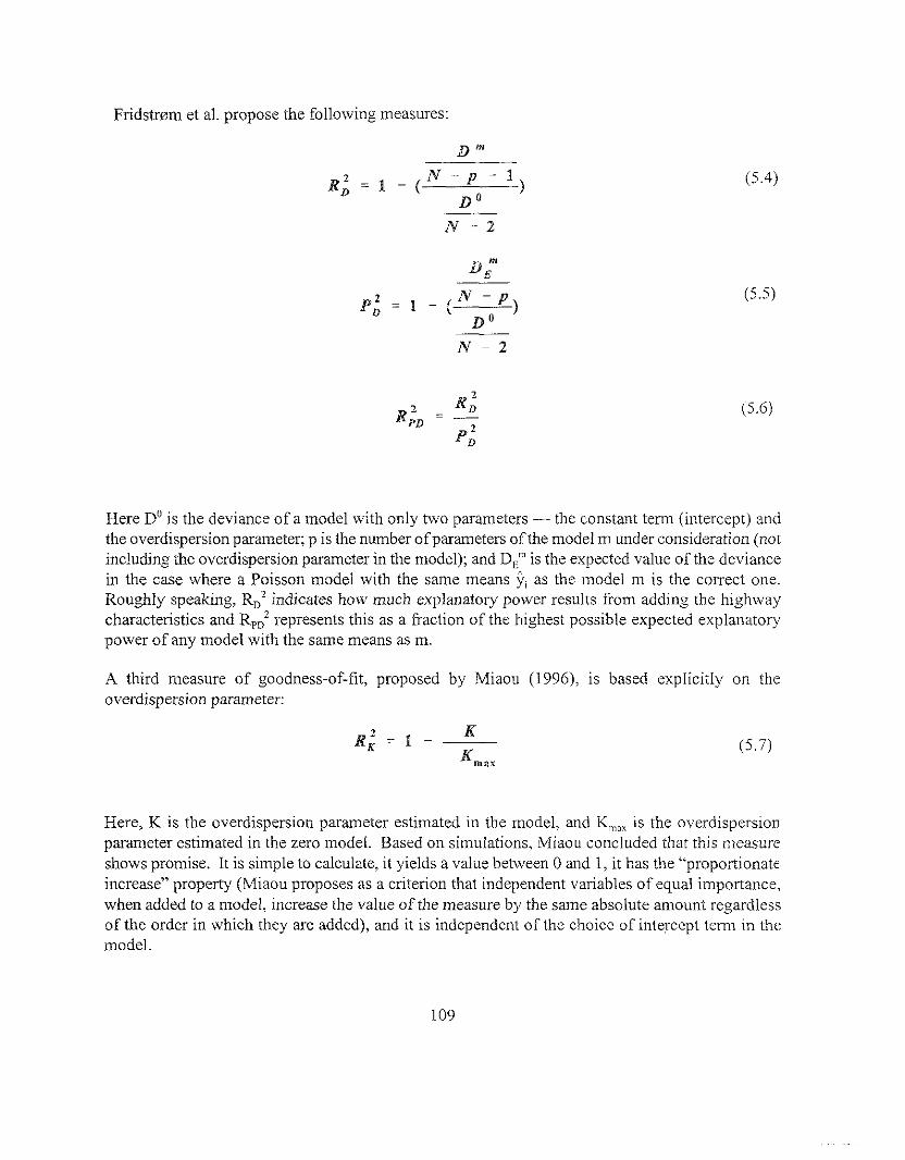
Fridstr@m et al. propose the following measures:
D“
N-2
N-2
2
R’=~PDP;
(5.4)
(j.5)
(5.6)
Here Do is the deviance of a model with only two parameters — the constant term (intercept) andthe overdispersion parameteL p is the number ofpararneters of the model m under consideration (notinchrting the overdispersion parameter in the model); and D~mis the expected value of the deviancein the case where a Poisson model with the same means yi as the model m is the correct one.Roughly speaking, R~2 indicates how much explanatoW power results from adding the highwaycharacteristics and RP~2represents this as a fraction of the highest possible expected explanatorypower of any model with the same means as m.
A third measure of goodness-of-fit, proposed by Miaou (1996), is based explicidy on theoverdispersion parameter:
(5,7)
Here, K is the overdispersion parameter estimated in the model, and Km.Xis the overdispersionparameter estimated in the zero model. Based on simulations, ~Miaouconcluded that this measureshows promise. It is simple to calculate, it yields a value between Oand 1, it has the “proportionateincrease” property (Miaou proposes as a criterion that independent variables of equal importance.,when added to a model, increase the value of the measure by the same absolute amount regardlessof the order in which they are added), and it is independent of the choice of intercept temr in themodel.
1.09
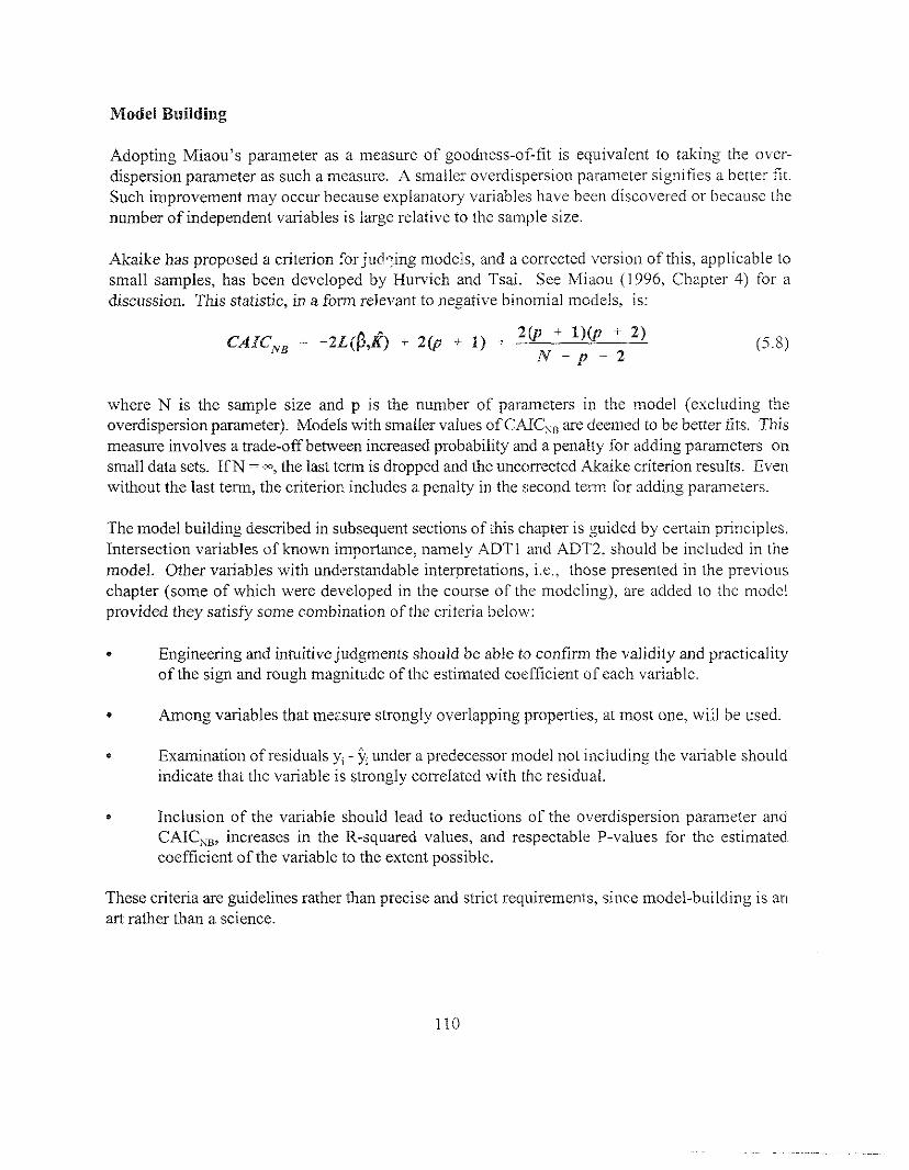
Model Building
Adopting Miaou’s parameter as a measure of goodness-of;fit is equivalent to taking the over-dispersion parameter as such a measure. A smaller overdispersion parameter signifies a better fit.Such improvement may occur because explanatory variables have been discovered or because thenumber of independent variables is large relative to the sample size.
Akaike has proposed a criterion for jud?ing models, and a corrected version of this, applicable tosmall samples, has been developed by Hurvich and Tsai. See Miaou (1996, Chapter 4) for adiscussion. This statistic, in a form relevant to negative binomial models, is:
(j,8)
where N is the sample size and p is the number of parameters in the model (excluding theoverdispersion parameter). Models with smaller values ofCAIC~~ are deemed to be better fits. Thismeasure involves a trade-off between increased probability and a penalty for adding parameters onsmall data sets. IfN = ~, the last term is dropped and the uncorrected Akaike criterion results. Evenwithout the last term, the criterion includes a penalty in the second tel-m for adding parameters.
The model building described in subsequent sections of this chapter is guided by certain principles.Intersection variables of known importance, namely ADT 1 and ADT2, should be included in themodel. Other variables with understandable inte~retations, i.e., thc,se presented in the previouschapter (some of which were developed in the course of the modeling), are added to the modelprovided they satisfy some combination of the criteria below:
e Engineering and intuitive judgments should be able to confirm the validity and practicalityof the sign and rough magnitude of the estimated coefficient of each variable.
e Among variables that measure strongly overlapping properties, at most one, will be used.
. Examination of residuals yi - $i under a predecessor model not including the variable shouldindicate that the variable is strongly correlated with the residual.
e Inclusion of the variable should lead to reductions of the overdispersion parameter and
CAIC~~, increases in the R-squared values, and respectable ?-values for the estimated.coefficient of the variable to the extent possible.
These criteria are guidelines rather than precise and strict requirements, since model-building is an@ rather than a science.
110

MODELS FOR TH~E-LEGGED INTERSECTIONS
Tables 28, 29, 30, and 31 show negative binomial models of crashes in terms of intersectionvariables for the three-legged intersections.
TABLE 28. Negative Binomial Models for Crashes pe!’ Year (TOTACC), Three-LeggedIntersections
Estimated regression coefficients (estimated standard error and P-value in parentheses).
Variables ADT On~y :=1Main M,>del
Intercept -12.9243 -12.2196 -12.2577(2.3682, 0.0001) (2.3575, 0.0001) (2.3626, 0.0001)
Log of ADTI 1.1989 1.1479 1.1778(0.2477, 0.0001) (0.2527, 0.0001) (0.2517, 0.0001 )
Log of ADT2 0.3027 0.2624 0.2034(0.0892, 0.0007) (0.0866, 0.0024) (0.1032, 0.0487)
MEDWIDTHI -0.0546 -0.0551(in feet), major road (0.0249, 0.0285) (0.0246, 0.0254)
NODRWI, 0.0391 0.0414driveways (0.0239, 0.1023) (0.0245, 0.091 2)to 250 ft, major road
PKYoLEFTI 0.0544major road (0.0471, 0.2479)
N, p 84,3 84,5 84,6
K Q.5256 (0.1366,0.0001) 0.3893 (0.1160,0.0008) 0.3658 (0.1095>0.0008)R; 0.5158 0.6413 0.6630
R2 0.2294 ‘ 0.4351 0.4473
R;, P; 0.1821,0.5628 0.2247, ~0.5589 0.2275,0.5524R;. 0.3237 0.4021 0.4119
CAIC.. 381.930 373.887 373.742
1 ft = 0.305 m
Table 28 indicates that the regression coefficient for (the 10200 maior road ADT is about four tOfive times that for minor road ADT, Among the next mos~ si~nificmt variables, as measured b!j
residuals after use of the ADT-only model, are NODRWY 1, MED WIDTH 1, and SPD 1. A second
111

TABLE 29. Negative Binomial Models for Crashes per Year (TOTACCI), Three-LeggedIntersections
Estimated regression coefficients (estimated standard error and P-value in parentheses).
Variables ADT only IMain Model Variant 1. Variant 2 Variant 3 1Intercept -16.1636 -15.4661 -16.6179 -15.700s -13.6339
(3.4655,0.0001) (3.4685,0.0001) (3.3126,0.0001) (3.3955,0.0001) (3.0516.0.0001)
Log 1.5023 1.4331 1.6117 1.4962 1.1954
of ADT1 (0.3s07, 0.0001) (0.3608,0.0001) (0.3s41>0.0001) (03s30. 0.0001) (0.3109>0.0001)’
Log 0.2904 0.2686 0.1276 0.1801 0.2646of ADT2 (0.1001,0.0037) (0.0988,0.006S) (0.1283,0.:1199) (0,,1187,0.1294) (o.lo~4>0.0091)’
MEDWIDTHI -0.0612 -0.06s7 -0.0607
ft (0.0360,0.0888) (0.0384,0.0738) (0.0340>0.0739)
NODRWYl 0.0560 0.0552 0.0597 0.0903
majOr road (0.0289,0.0S2S) (0.0290,0.0S65) (0.0283,0.03S0) (0.0266.0.0007!
PK%TUW 0.0401(0.021s, 0.0617)
PKYoLEFTI, 0.0764major road (0.0665,0.2S09)
VEI-1, vertical 0.1180OUt to 800 ft, (0.0700,0.0919)
major road4
HAU
J - J
0.0197angle (0.0174,0.2S91)
N, p 84,3 84,5 84,6 S4, 6 S4, 6
K 0.7332 0.s118 0.4195 0.4416 0.4416(0.2068,0.0004) (0.1719,0.0029) (0.1478,0.0046) (0’.1s13,0.003s) {0.1642,0.0072)
R; 0.5139 0.6607 0.7072 0.70720.7219
R2 0.1666 0.4452 0.4644 0.4757 0.4287
R;, P; 0.1731,0.S322 0.2233,0.S374 0.2491,0.53S6 0.2371,0.S313 0.2278, 0.5196
R;. 0.3253 0.4155 0.4652 0.4462 0.4384
CAIC.. 326.27S 317.141 313.620 315.s00 317.4s0
1 ft = 0.305 m
112

TABLE 30. Negative Binomial Models for Crashes per Year (l NJACC), Three-LeggedIntersectiosss
Estimated regression coefficients (estimated standard error and P-value in parentheses).
Variables ADT On~~
‘aria~
Intercept -13.1685 -12.3246 -11.0061
(3.0319, 0.0001) (2. S0’76, 0.0001) (2.6937,0 .0001)
Log of ADTI 1.202s 1.1436 0.9526(0.3082, 0.0001) (0.2763, 0.0001) (0.2S43, 0.0008)
Log of ADT2 0.1925 0.1357 0.1499(0.0931, 0.03ss) (0.1029, 0.1 872) (0.0916, 0.1018)
HAU 0.0230 0.0289
~ngle (0.01 31, 0.0790) (0.01 05, 0.0061)—
YODRWYl, driveways 0.0481out to 250 ft, major road (0.0262, 0.0664)
—
ABSGRDI, average 0.1S38grade, major road (0.1130, 0.103s)
N, p S4, 3 84,4 S4, 6—
K 0.5649 (0.z032,0.0055) 0.3787 (0.1792,0.0346) 0.258S (0.1848,0,1613)R~ 0.4535 0.63:16 0.7496
R2 0.1400 0.3755 0.4505
R;, P; 0.1437,0.4039 0.1S41, 0.3966 0.2036, 0.3S37
R;D 0.355s 0.4644 0.5306
CAIC~~ 274.653 269.275 26 S.0S1
ft= 0.305 m
tier of significant vtiables includes PKYOTRUCK and LTLN 1. All of these vatiables correla[e withNODRfiY 1 and MEDWIDTH1 (see Table 18), and when the latter two variables are added, theothers become much less significant. However, it is also tru[>that NODRWY 1 and MED WIDTH 1correlate strongly with each other (correlation coefficient -0.37654 and P-value 0.0004).
Nonetheless, we keep them both because they seem to have separate effects in the mtin model o<Table 28. When we consider residuals for the main model, the angle variables DEV and HAU shov,positive correlation, as do turning percentage variables. If we add an angle variable and a turningpercentage variable to the model, the overdispersion parameter K reduces to about 0.29, but the P-
113
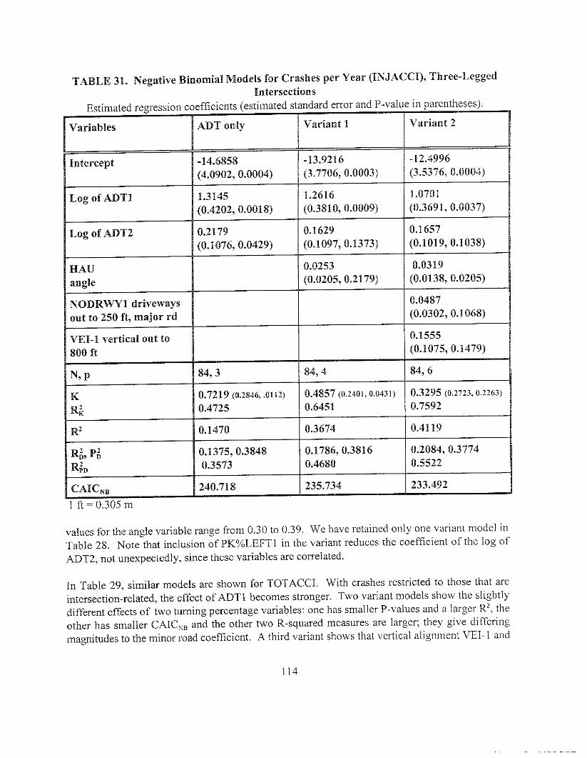
TABLE 31. Negative Binomial Models for Crashes pe!r Year (INJACCI), Tl~ree-LeggedIntersections
Estimated regression coefficients (estimated standard error and P-value in parentheses).
Variables ADT O~]y —~]Varia~t 1
! 1
Intercept -14.6858 -13.9216 -12.4996
(4.0902, 0.0004) (3.7706, 0.0003) (3.5376, 0.0004)
Log of ADTI 1.3145 1.2616 ?.0701(0.4202, 0.0018) [0.3810, 0.0009) (0.3691 , 0.0037)
Log of ADT2 0.2179 0.1629 0.1657(0.1076, 0.0429) (0.1097, 0.1373) (0.1019, 0.103s)
HAU 0.0253 0.03s9angle (0.0205, 0.2179) (0.0138, 0.0205)
NODRWYl driveways 0.0487out to 250 ft, major rd (0.0302, 0.1068)
VEI-I vertica~ out to 0.1555Soo ft (0.1075, 0.1479)
N, p 84,3 S4, 4 84,6
K 0.7219 (0.2846, ,01 12) 0.4857 (0.2401, 0.(1431) 0.3295 (0.2723. 0.2263)
R; 0.4725 0.6451 0.7592
R’ 0.1470 0.3674 0.4119
R;, P; 0.1375, 0.384S 0.1786, 0.3S16 0.20S4, 0.3774R;. 0.3573 0.4680 0.5522
CAICN. 240.718 235.734 233.492
[ ft = 0.305 m
values for the angle variable range from 0.30 to 0.39. We have retained only one variant model ill-.
Table 28. Note-that inclusion of PKOALEFTl in the variant reduces the c~efficient of the log ofADT2, not unexpectedly, since these variables are correlated.
In Table 29, similar models are shown for TOTACCI. With crashes restricted to those that areintersection-related, the effect of ADT 1 becomes stronger. Two variant models show the slightlydifferent effects of two turning percentage variables: one has smaller P-values and a larger R2, theother has smaller CAICK~ and the other two R-squared measures are largeL they give differingmagnitudes to the minor mad coefficient. A third variant shows that vertical alignment VE1- 1 and
114

the angle variable HAU in a suitable combination, but not without each other, have some explanatoryvalue in place of MED WIDTH 1.
When we turn to serious crashes (INJACC and INJACCI) i:t Tables 30 and 31, the importance ofADT1 relative to ADT2 continues to increase. In addition, h4EDWIETH 1 ceases to be significantand HALT becomes an important variable. Recall from Figures 2 and 3 that the sign of HAU ispositive when a driver turning from the major road across traffic need only turn through a smallangle. According to these models, this increases crashes This suggests that perhaps the morerelevant movement is turning from the minor road. A driver ‘turning right from the minor road mayhave the iIlusiorr of easy access, but inadequate visibility for traffic on the major road traveling inthe same direction, while a driver turning left will have poor visibility of the tmffic that must becrossed. Only 17V0of the three-legged intersections had HAU different from zero (cE Table 5), andthe ones with HAU higher than zero had more inju~ crashes than average and the ones with HAUlower than zero had fewer crashes. Recall from Table 11 that HAU has a strong positive correlationwith all crash types. With MEDWIDTH 1 removed and tIAU added, NODRW 1 and one o f the twovertical alignment variables VEI- 1 or ABSGRD 1 also contribute to injury crashes in the othermodels shown in Tables 30 and 31.
Variables not included in these models, such as STATE, sight disl.anccs, and HE1-I. had veryinsignificant P-values after inclusion of the variables shown in the tables.
The three-legged models have the following general features:
. TOTACC and TOTACCI models are similar, INJACC and INJACCI models are simi Iar.
. For all four crash variables, ADT 1, ADT2, and NOI>RWY 1 are influential
. For TOTACC and TOTACCI, MEDWIDTH 1 and turning percentage are influential
. For INJACC and NJACCI, the angle variable HAU and vertical alignment are influential,and, to some extent, this is also true for TOTACCI.
MODELS FOR FOUR-LEGGED INTERSECTIONS
The models for the four-legged intersections are exhibited in Tables 32, 33, and 34
Table 32 shows models for TOTACC. In the absence of other variables, minor mad ADT appearsto be more influential than major mad ADT. When other variables are added, in particular, tumi n;:and through percentages, ADT 1 becomes much more influential than ADT2. The variables thatcorrelate most strongly with the residuals of the ADT-only model are RSDR2, PKO/oLEFT1,LTLNI S, and STATE, in order. However, when these variables are added to the models, the onesthat are most significant are PKOALEFT1 and LTLN 1S. Both of them correlate strongly with
115

TABLE 32. Negative Binomial Models for Crashes pt;r Year (TOTACC), Four-LeggedIntersections
Estimated regression coefficients (estimated standard error and P-value in parentheses).
Variables ADT only Main Model Variant 1 Variant 2 Variant 31
Intercept -6.9352 -9.46311 -10.1902! -10.9526 -9.7859(2.3767,0.0035) (2.5991, 0.0003) (3.3126,0.0021) (2.5907,0.0001) (2.6032,0.000:2)
Log 0.4683 0.8503 0.8873 1.0382 0.8s94
of ADTl (0.2330,0.0444) (0.2779,0.0022) (0.2653,0.0008) (0.2870,0.0003) (0.2873.0.00211)
Log 0.5135 0.3294 0.2924 0.2206 0.284j
of ADT2 (0.0896,0.0001) (0.1255,0.0087) (0.1316,0.0263) (0.1219,0.0704) (0.1375,0.0385)
PKY”LEFTI, 0.1100 0.2976 0.1054
major road (0.0412,0.0076) (0.1393,0.0326) (0.0372,0.0046)
LTLNIS -0.4841 -0.6607 -0.5471(O or 1) (0.2311,0.0362) (0.2347,0.0049) (0.2445,0.0252)
PK%LEFTI -0.0131squared (0.0094,0.1643)
PKYOTHRU2 0.0220minor road (0.0107,0.0391)
ABSGRDI 0.1553major road (0.1123,0.1666)
PK%,TURN 0.0351(0.0238,0.1404)
100 XRSDM 2.2s4
(looxl/ft) 1 ft = 0.305m (1.503,0.1286)
N, p 72,3 72,5 72,5 ’70,1 72,6
K 0.6144 0.4578 0.4S20 0.36s2 0.41s3\ (0.156z,0.0001) (0.1307,0.0005) (0.1425,0.0007) (0.1124,0.0011) (0.1147,0.0003)
R; 0.3s01 0.53s1 0.5136 0.5953 0.5780
R2 0.2565 0.3109 0.2520 0.4797 0.4494
R;, P; 0.10S0, 0.6011 0.1623,0.5S58 0.2557,10.5874 0.1575,0.5666 0.1635,0.57’?2
R;. 0.1796 0.2771 0.2557 0.27S0 0.2s22
CAICX, 385.16S 374.94s 377.165 369.S29 374.870
116

TABLE 33. Negative Binomial Models for Crashes per Year (TOTACCI), Four-LeggedIntersections
Estimated regression coefficients (estimated standard error and P-value in parentheses).
FFLogof mTl
Logof ADT2
PKYoLEFTImajor road
LTLNIS(0 or 1)
PKOALEFTlsquared
PK%THRU2minor road
ABSG~lmajor road
N, p
LK
R;
L
ADT On~~ Main MOdel Variant 1 Variant 2 Variant 3
, ,
-7.2501 -11.1096 -1(].9008 -? 1.8796 -13.28C5 =(2.9094,0.0130) (3.3345,0.0008) (3.3257,00010) (3.2980,0.0004) (3.2833,0.0001.)
0.4582 0.9299 0.9325 1.0161 1.2160(0.2844,0.1071) (0.3433,0.0067) (0.3452,00069) (0.3382,0.0027) (0.3434,0.0004)
0.5311 0.3536 0.3498 0.2866 0.2195(0.0996,0.0001) (0.1163,0.0024) (0.1300,00071) (0.1336,0.0319) (0.1279,0.086~!)
0.1491 0.1427 0.3854 0.1396(0.0586,0.0110) (0.0583,0,0144) (0.1674,0.0213) (0.0540, 0.009:7)
-0.2891 -0.4890(0.2920,0.3222) (0.2970,0.099[1)
-0.0172(0.0111,0.1221)
—
0.0284(0.0145,0.051‘r)
—
0.1698(0.1353,0.2093)
72,3 72,4 72,5 72, 5 70,7—
1.8814 0.7096 0.6901 0.6548 0.5556‘0.2267,0.0001) (0.1906,0.0002) (0.1827,0.0002) (0.1779,0.0002) (0.1512,0.0002)).3338 0.4.637 0.4784 0.5051 0.5498
—
1.2323 0.1587 0.1952 0.1646 0.3675
).0814, 0.5802 0.1334, 0.571s 0.1273, 01.Sb46 0.1410,0.5665 0.1275,0.5470).1403 0.2334 0.2255 0.248S 0.2332
——
!50.ss7 341.404 342.S41 340.13s 337.S89
117

TABLE 34. Negative Binomial ModeIs for Crashes per Year (INJACC and INJACCl),Four-Legged Intersections
Estimated regression coefficients (estimated standard error and J’-value in parentheses).
Log of ADT2 0.4778 0.3237 0.5138 0.3310(0.1401,0.0007) (0.1645,0.0491] (0.1604,0.0014) (0,1894, 0.0805)
PKYoLEFTI 0.0994 0.1228major road (0.0433,0.0216) (0.0614,0.0457)
SPD2 0.0339 0.0429(in mph) (0.0179,0.0577) (0.0240,0.0740)
N, p 72,3 12,5 72,3 I 72,5
K 0.5741 0.4308 0.9671 0.7178(0.1821,0.0016) (0.1824,0.0182) (0.2899,0.0009) (0.2716,0.0082)
R& 0.4218 0.5662 0.3449 0.5138
R* 0.2445 0.3565 0.1987 0.3237
R;, P; 0.1197,0.4817 0.1550,0.4654 0.0834,0.4812 0.1214,0.4680
R;, 0.2485 0.3331 0.”1734 0.2593
CAIC., 294.271 289.919 275.196 270.302
1 mph= 1.61 km/h
STATE, ad STATE ceases to correlate significantly i~ith the residual of this new model.PKOALEFTl and LTLNI S correlate \vith each other as well, having a correlation coefficient of-0.22S8 and a P-value of 0.0532, but both of them still seem to contribute to the accident count.
The original major road iefr-tum lane variable LTLN1 t~es values O, 1, and 2, but only 4 out of 72four-legged intersections (see table 6) have exactly one left-turn lane. One can model the left-turnlanes on the major road using two regression coefficients (dividing the intersections into threesubclasses), but the quantity of data does not support this option. If one uses only the variableLTLN1, one is adopting the bias that two turning lanes ha,~e double the safety effect of one. Our
118
data suggest that two left-turning lanes are less safe than one: :1model with coefficients for each casegives a larger negative coefficient when there is one turning lane than when there are two. Thevariable LTLN1 S takes the value 1 when there is at least o~le lefi-tuming lane on the major road.This, in effect, divides the intersections into two classes and avoids any assumptions about therelative safety of intersections with one versus two left-turning lanes. (A similar approach is usedin the next section with the signalized data where PROT_LT indicates at least one protected left turnon the major road.) Variant 1 is a model that indicates a quadratic dependence of crash count onPKY.LEFT1. This model does not perform as well as the main model, but is present becauseresiduals for the main model correlate negatively with PKO/oLEFT1. We will discuss this issuefurther in collection with TabIe 33. If LTLNI S is added tc, the Variant 1 model of Table 32, thequadratic term in PK%LEFT1 becomes insignificant, with a P-value going to 0.3962.
The next most significant variable afier those in the main model is PK0ATHRU2. There are reasonsto be wary of adding two turning percentages because of the strong correlations among ADT 1,ADT2, PKYoLEFT1, and PK0ALEFT2 (see Tables 16 and 19). Also, two intersections must beremoved from the sample for which the minor legs had no traffic approaching the intersection duringthe peak-hour visits. However, if PKO/0THRU2 is added, it is significant. The design variableABSG~l is also included in Variant 2.
Variant 3 in Table 32 is obtained by using PKO/.TURN rather than PK.”/oLEFT1 and proceeding toadd significant variables. The average sight distance right from the minor mad in feet, representedhere by its reciprocal multiplied by 100, is known to be correlated with all types of crashes (seeTable 12). Also, it has a strong correlation with tbe residuals from other models, but when it isadded to models, Variant 3 is the only model where its regression coefficient achieves a relativelysmall P-value.
In Table 33, similar models are done for TOTACCI. The results are similar except that LTLNI Sis less significant. A version of Table 32, Variant 3, is not shown because the P-values of LTLN 1Sand RSDR2 rise from 0.0252 and 0.1286 to 0.2594 and 0.3 [08, respectively.
We discern again a quadratic dependency on PKYoLEFTI (compare Variant 2 in Table 33 withVariant 1 in Table 32). A quadratic of the form ax - bx2 with a and b positive has its mmimum when.~ = ~2b, The two quadratic models have maximum contribution from PKO/OLEFT1 at the values
0.2976/(2x0.01 31) = 11.36 and 0.3854/(2x0.0172) = 11.20, respectively. This suggests that wher.the left-turn percentage from the major road is less than 110/0, crashes rise with increasingpercentage, but that when it is greater, crashes fall with increasing percentage. Among the 72intersections upon which the model is based, 5 of them have PKO/”LEFTl in excess of 11O/..
Variant 1 in Table 33 includes LTLNI S, and yields Improvement In K and Rz, bat not in R~,,,ol-
CAICK” or P-values. Likewise, Variant 3 in Table 33 includes the design variables LTLN I S andAB SGRD 1. Without them, but with PKY.LEFT 1 and PKV.THRU2 retained, in a model forTOTACCI that we do not display, the overdispersion parameter K is larger (O.6261), R2 is smaller(0. 1260), and R~ is smaller (0.2261), but CAICXBis also smaller (337.641 ). This is a reminder that
119

the various criteria do not always have consistent trends. In addition, the behavior of CAICX,I~ugge~ts the possibility that a regime is being entered where overfitting occurs. overfitting occurs
when random variation in a set of input variables is USedto explain the random variation in a singleoutput variable. When the number of input variables is a significant: fraction of the sample size,some combination of the noises in the input variables may, by coincidence, approxilllate tilevariation in the output variable without having predictive value.
Models for INJACC and NJACC1 are shown ‘UTable 34. Turning percentages are significant forthese models and so is posted miuor road speed SPD2, but other design variables fail to be.PKY0THRU2 is marginally significant with a P-value of about 0.19, but it has been omitted, in part,because the interpretsstion is unclear. Since SPD2 correlates negatively with STATE, one mightsuspect that its influence is due to that source, but STATE itself is ]qot significant in tbe presence ofthe ADT variables and PKY.LEFT1.
The general features of the models for the foLLr-leggedinter~ectiOns are:
. Turning percentage, along with major and minor mad ADT, are influential for all crashtyQes.
. LTLh~l S, which registers the presence of one or more left-turn lanes on the major road, isinfluential for TOTACC and marginally so for TOT.4CC1.
. Grade and poor sight distance right from the minor road are marginally significant forTOTACC and TOTACCL
. High minor road posted speed appears to contribute to serious crashes.
MODELS FOR THE SIGNALIZED INTERSECTIONS
Negative Binomial Models
The signalized intersectimls present special difficulties As shown in Table 26 and Figure 9, at RI:
appearances, the dependence of crashes on major road ADT i.snegligible, Likewise, the correlatlo~.
coefficient between crashes and ADT 1 is insignificant in Table 1~. An ADT-only model forTOTACC in terms of the logs of ADT1 and ADT2 actually assigns a negative (but insignificant)regression coefficient to the log of ADT 1.
Part of the insignificance perhaps stems from the small sample size — only 49 signalizedintersections. However, at signalized intersections, minor and major roads tend to have more equalstanding. If their standing is equal, their ADT’s should enter into any model symmetrically. Forexample, the coefficient of ADT 1 would be the same as that of ADT2 except for noise. We ~aveattempted to address that possibility by using the log of the product, log(ADT 1xADT2), as a vartabl(:
120

in some of the signalized models below. At the same time, ADT by itself becomes less important.Signalized intersections, one may argue, are less stereotypical than other rural intersections. On thelatter, the division between major road and minor road is more pronounced and the turningpercentages on each fall into a narrower range. More important on the signalized intersections, oncwould judge, are the movements of the vehicles through the intersection. Turning percentages, leftand right, from all approaches and flows along each approach are likely to be more determinativeof crashes.
There is also the issue of how to define the major road. Usually, and in this study, it is taken to bethe road with the larger ADT. But if there is significant turning along certain legs, legs of the sameroad may have drastically different ADT. Most of the ADT may be on two adj scent legs, say legs1 and 4, and very little on the other two adjacent legs, legs 2 and 3. See Figure 1. Usually, the majorroad has a lower percentage of turning traffic than the minor road, but it is possible that a road withless traffic would have virtually no turning traffic (all of it through), while the crossroad has muchmore traffic and a significant amount of it is turning. In the data, an asymmetry can occur betweenminor road turning traffic and major road turning traffic. ‘This can be caused by failure of themorning and evening peak hours to match up, by unusual travel hours to and from locations, or evenby alternative routes.
Despite these considerations, the models exhibited here take ADT to be primary, in part because ofits familiarity and acceptability to the engineering community and in part to permit comparisons withother models that use ADT. Yet, it should be recognized that rural signalized intersections are atransitional class where variables other than ADT may prove to be more appropriate. This isaddressed in the subsection afier this one, where models of single and mu)tiple-vehicle crashes interms of traffic flows are briefly investigated.
In Tables 35, 36, and 37 are shown negative binomial models for crashes on the signalized two-laneby two-lane intersections. ADT-only models are omitted since when ADT1 and ADT2 areseparated, ADT 1 is insignificant and has a coefficient of negative sign, and when they are united inthe form log(ADTl xADT2), the model coefficients are somewhat unstable (SAS and LIMDEP giverather different values for the regression coefficients, but the same 10S I.ikelihood, indicating that themmimum occurs at a hard-to-find set of values on a large relatively flat plateau). When variablesthat correlate well with the residuals to these models are added, the models settle dow and the ADTvariables share in the significance.
Table 35 shows models for TOTACC. The existence of one or more protected left turns on themajor road at the signal is an influential variable. It correlates strongly with STATE, as no{edearlier, and it is possible that there is a combined effect here. A total of 17 out of 18 Californiasignalized intersections had one or more protected left turns on the major road, whi Ie only 4 out of31 Michigan signalized intersections did. Nonetheless, when PROT_LT is added to the mode)versus STATE, the former improves the model more than the latter, and the correlation between theresidual of a PROT_LT model and the STATE variable is negligible.
121

TABLE 35. Negative Binomial Models for Crashes per Year (TOTACC), SignalizedIntersections
Estimated regression coefficients (estimated standard error ad P-value in parentheses).
[Variables Main Model Variant 1
‘ar~
Intercept -6.9536 -6.1236 -6.3658 -5.4091(2.7911,0.0132) [2.5973,0.0184) (3.3207,0.0S52) (3.0054.0.0718)
Log of ADTI 0.6199 0.6475(0.2504,0.0133) (0.3156,0.0402)
Log OfADT2 0.3948 0.2104(0.1737,0.0230) (0.2232,0.3459)
Log of 0.4643 0.3914ADTI xADT2 (0.1483,0.0017) (0.1732,0.0238)
PROT_LT -0.6754 -0.6110 -0.7181 -0.5980O=no, l=yes (0.1S24!0.QO02) (0.1507,0.0001) (0.1973,0.0003) (0.1690,0.0004)
PK”/oLEFT2 -0.0142 -0.0134 rminor road (0.0047,0.0023) (0.0048,0.0052)
PK”ALE~l 0.0220 0.0137major road (0.0”142,0.1207) (0.0116,0.2388)
VEICOM 0.1299 0.1243 0.1001 0.1044vertical, all (0.0450,0.0039) (0.0507,0.0142) (0.0508,0.0486) (0.0618,0.0914)
legs
PKY”TRUCK 0.0315 0.0300 0.0353 0.0317truck ‘~. (0.0143,0.027S) (0.0141,0.0331) (0.0175,0.0441) (0.0167,0.0573)
N, p 49,7 49,6 49,7 49, 6
K 0.1161 0.1186 0.1353 0.1422(0.0323,0.0003) (0.0317,0.0002) (0.0341,0.000i) (0.0375,0.0002)
R; 0.6490 0.6414 0.5910 0.5701
R2 0.5053 0.5208 0.5134 0.5172
R;, P; 0.1479,0.6262 0.1619,0.6349 0.1059, 0.&163 0.1123,0.6351R;. 0.2362 0.2550 0.1691 0.1768
CAIC.,, 358.508 356.471 363.937 363.044
122

TABLE 36. Negative Binomial Models for Crashes pt~r Year (TOTACCI), SignalizedIntersections
Estimated regression coefficients (estimated standard emor and P-va!ue in parentheses).
Variables Main JModel Variant 1 Variant 2 Variant 3
Intercept -6.0841 -4.9564 -4.1075 -5.4581(3.3865,0.0724) (3.0779,0.1074) (2.9461,0.1633) (3.1937,0.0874)
Log of ADTl 0.5951 I 0.5995(0.2847,0.0366) (0.2795,0.0319)
Log of ADT2 0.2935 0.2015(0.1972,0.1366) (0.1917, 0.2932)
Log of 0.3857 0.3320ADTI xADT2 (0.1788,0.0309) (0.1’719,0.0534)
PRQT_LT -0.4708 -0.3822 -0.3025 -0.4041O=no, l=yes (o.zooo>o.o18~) (0.1668,0.0220) (0.1745,0.0830) (0.1883,0.0319)
PKY”LEFT2 -0.0165 -0.0153 -0.0160 -0.0177minor road (0.0057,0.0036) (0.0060,0.0101) [0.0055,o.oo3a) (0.0050,0.0005)
VEICOM 0.1126 0.1033 0.0996 0.1114vertical, (0.0365,0.0020) (0.0416,0.0130) (0.0382,0.0091) (0.0326.0.0006)
all legs
PKYoTRUCK 0.0289 0.0268 0.0234 0.0256truck 0/. (0.0131,0.0276) (0.0131,0.0398) (0.0122,0.0j47) (0.0117,0.0287)
NODRWI 0.0347 0.0407major road (0.0270,0.1986) (0.0246,0.0983)
N, p 49,7 49,6 49,7 49,8
K 0.1313 0.1354 0.1222 0.1145(0.0392,0.0008) (0.0390,0.0005) (0.C1374,0.0011) (0.0401,0.0043)
R; 0.5521 0.5382 0.5834 0.6094
R2 0.3650 0.3913 0.4563 0.4327
R;, P; 0.0944,0.5854
~i~~ ‘::*
0.1053,0.5951R;. 0.1612
CAIC., 342.266
123

TABLE 37. Negative Binomial Models for Crashes ~ler Year [INJACC, INJACCI),Signalized Intersections
Estimated regression coefficients (estimated standard e:mor and P-valL——
Variables INJACC INJACC1
Intercept -3.2562 -:[.547s(2.9932,0.2767) (3.0298,0.6095)
Log of 0.2358 0.1290ADTI xADT2 (0.1722,0.1707) ((1.1757,0.4627)
PRoT_LT -0.2943O=no,l=yes (o1864,~l144)
PKY”LEFT2 -0.0113 -0.0149minor road (0.0062,0.067ti (0.0066,0.0250)
VEICOM 0.0822 0.0686verticai, (0.0551,0.1358) (0.0692,0.18j8)
al! Iegs
PKYoTRUCK 0.0323 0.0282trfitck ‘/. (0.0146,0.0267) (().0152,0.0628)
——N, p 49,6 49, s
K 0.1630 0.1433(0.0662,0.0138) ({}.0692,0.038j)
R; 0.4474 0.4829
R’ 0.3275 0.3488
R;,, P; 0.0420,0.4926 0.066S, 0.456SR;” 0.08S3 0.14S8
CAIC~~ 28 S.287 265.687 ,
in parentheses).
Other significant vtiables shown in the main model of Table 35 include PKYoTRUCK, VEICOM,and PKO/.LEFT2.
Crashes rise at signalized intersections with a higher percentage of truck traffic and with morevertical cuwature out to 800 feet (244 meters) on any or all approaches. Trucks at a signal, as wellas having greater destructive capacity than passenger vehicles, take a long time to engage in turning;maneuvers and block visibility during this time. In Table 13, almost all vertical variables correlatepositively with crashes, although few have significmt P-~alues. The combination that is mosl:
124
significmt in the modeling is VEICOM. VEICOM is an average change of grade per 100 feet (30.5meters) along both major and minor roads for vertical curves at least partly within 800 feet (244meters) of the intersection center. One may wonder why VEICOM is more significant than VICOM,the comparable measure out to 250 feet (76 meters). Signalized intersections are mrely placedimmediately beside vertical curves, but are often found to be displaced from them by hundreds ofyards or meters. The mean, median, and standard deviation of VICOM are 1.79, 1.2, and 0.28,respectively, while those for VEICOM are 1.88, 1.43, and 0.27. The difference in medians, inparticular, shows that vertical curves partly within 800 feet (244 meters) of the intersection, b:..! ,:o!within 250 feet (76 meters), increase the average.
Crashes fall with increasing PK%LEFT2, the left-turn percentage on the minor road. PK%LEFT2is the most significant of the turning percentage variables, but the others are also significant.PKY0LEFT2 is, of course, equivalent to (100 - PK0ATHRU2 - PK0ARIGHT2), i.e., to the sum ofPKY0THRU2 and PKY.RIGHT2, ad each of the latter two vmiables correlates positively withcrashes (see Table 23). PKO/0LEFT2 correlates negatively with PKO/OLEFT1 and thus the lattershould increase crashes. Variants 2 and 3 in Table 35 show that this is indeed the case, but that theP-value rises. Note also that the P-value for the log of ADr2 becomes rather large in Variant 2,presumably due to the strong positive correlation between PKVOLEFT1 and ADT2 (Table 17).
The difference between the Main Model in Table 3S and Variant 1 is in the use ofLog(ADTI xADT2) rather than the individual logs. In fact, Variant 1 gives a smaller value ofCAIC., and a larger value of R2. The decrease in CAIC,,I suggests that Variant 1 may be thesuperior model: it has about the same explanatory value, but with fewer variables. 10 the MainModel, we have elected to exhibit coefficients for ADT 1 and ADT2 separately, partly to allowcomparison with other models, When they are combined in Variant 1, the new coefficient isintermediate between the separate coefficients. The estimated difference in tbe two coefficients inthe Main Model is, of course, 0.6199-0.3948 = 0.2251. ‘Using the estimated covariance matrix forthe model, we find that the estimated standard error of the estimated difference is [(0.2 S04)Z +(0. 1737)2 - 2X0.0039226]”2 = 0.2916. This gives a P-value of 0.4401 for testing the hypothesis thatthe coefficients are different. In other words, the Main Model does not alIow us to reject the
hypothesis that the regression coefficients of the logs of ADT1 and ADT2 are the same.
The models for TOTACCI in Table 36 are similar to those in Table 35, except that the P-value of
ADT2 increases and the variable NODRW1 is marginally significant in Variant 2 and significant.in Variant 3. Variant 3 has m unacceptably high P-value for .~T2. NODRWY2 and the combined.variable NODRWCOM, although positively correlated with crashes, do not achieve as good a P.value as NODRWY 1. NODRWY 1 also correlates positively with TOTACC, and in a TOTACCmodel with the same variables as Variant 2 of Table 36, gives a P-value of 0,2270. Surprisingly,its P-value in Variant 2 of Table 36, 0,1986, is lower, This is a surprise because TOTACCI attemptsto eliminate driveway crashes with no intersection involvement. We have omitted variant model$sin which PKO/.LEFTl is used instead of PKO/oLEFT2. In (one such model, the P-value of ADT2jumps to 0.6481, although other vtiables behave well; in another mo(iel with LOG(ADTI xADT2),ADT behaves well, but VEICOM and PK%LEFT1 have P-values of 0.2402 and ().3263,
J25

respectively.
For boti TOTACC and TOTACCI, variables such as LIGNr and LTLNl correlate well with theresiduals of the models shown, LIGHT positively and LTLN1 negatively. When these variables areadded to the models, they are also marginally significant. Holvever, the values of CAICYUdo notdecrease, and concern about overtitting leads us to omit them.
In Table 37, we present one model each for INJACC and ~JACCL The coefficient of the log ofADT2 is quite insia~ificant because of large standard error. So we only exhibit models usingLOG(~Tl xDT2). Even with these, the P-value deteriorates substantially. In addition, VEICOMbecomes less significant and PROT_LT attains, in the case of rNJACCI, a P-value of 0.5666 (notshown).
The main features of the signalized intersection models are:
. ~Tl is insignificant for all crash types when ADT2 is present but without other variables.
. PKVOTRUCK and the turning percentages, especially PK0ALEFT2, are significant fot- allcrash types.
. The existence of one or more protected left turns on the major road, as \vell as major and
minor road vertical curves, is significant for TOTACC ancl TOTACCI, becoming lesssignificant for INJACC and insignificant for IN-JACCI.
o NODRWY 1 is marginally significant for TOTACC and TOTACCI, but not for seriousaccidents.
e For TOTACC and TOTACCI models, in general, ADT 1 becomes more significant asvariables are added, while ADT2 gets less significant, sharing its influence with turnin~,percentage.
Flow Models
The signalized intersections, as noted, behave somewhat peculiarly with respect to ADT. Thissuggests a more detailed analysis, making use of flows and crash types. Here we examine a fevmodels based on the decomposition of TOTACC into single-vehicle crashes and multiple-vehicl~:crashes by the variables TOTACCS and TOTACCM. Although many single-vehicle crashes ma!{in fact be multiple-vehicle crashes in which other vehicles (escape unscathed, we proceed as if thi jdecomposition is valid.
For single-vehicle crashes, one approach is to regard them as functions of incoming flows, wit.1minor and major legs treated on an equal footing and without interaction terms. An underlyingrationale is that single-vehicle crashes depend on same-direction traffic as well as intersection
126

features ether than traffic, such features including perhaps pedestrian traffic, intersection geometry,roadside huards, obstructions that limit sight diseances, signal timing, etc. Theo one might expectthat the number of such crashes is proportional to some power of the flow. Although such a viewis not particularly consistent with the evidence in Table 21, we pursue the approach and indicate theoutcome.
A negative binomial model with mean number ofsingle-vellicle crashes per unit time ofthe form
is sought with varimce equal to y + Ky2. The unknowns are the multiplicative constant C, thepower a, and the overdispersion parameter K. For a given power a, LIMDEP or SAS wilI choosethe pair (C, K) to maximize the probability (or log-likelihood) of the observed numbers y of single-vehicle crashes given the observed values of F,, Fz, F3, and Fq. The crude strategy we follow,suggested by the measure R? , is to vary a and choose the triple (C, a, K) that yields the smallestvalue for K (and hence the largest for R;).
When this is done, the resulting model is as follows:
SINGLE-VEHICLE CWSH MODEL. SIGNALIZED INTERSECTIONS
wherew is the mean number of single-vehicle crashes per yem,
the intersection flows are FI, F2 F,, and F, in thousands of vehicles per day, and
the overdispcrsion parameter K = 0.4670.
The constant term -1.9218 has an estimated standard errorcfO.1419 and a P-value of 0.0001, andthe overdispersion parameter 0.4670 has an estimated standard error of 0.1993 and a P-value of0.0192. Because of the modeling technique, an estimated standard error for the power a = 0.01 isnot available.
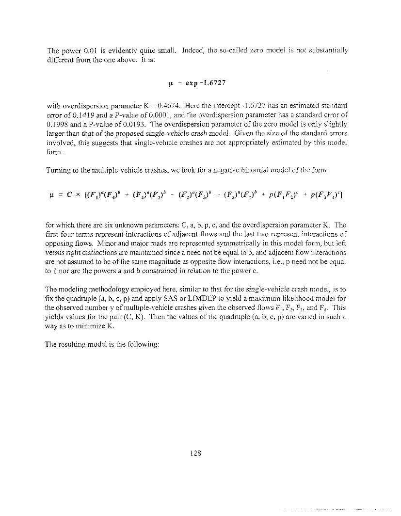
The power 0.01 is evidently quite small. Indeed, the so-tailed zero model is not substantiallydifferent from the one above. It is:
p = exp-1,6727
with overdispersion parameter K = 0.4674. Here the intercept -1.6727 has an estimated standarderror of0,1419 and a P-value of 0.0001, and f!le overdispersion parameter has a standard error of0.1998 aud a P-value of 0.0193. The overdispersion parameter of the zero model is only slightlylarger thm that of the proposed single-vehicIe crash model. Given the size of the standard errorsinvolved, this suggests that single-vehicle crashes are not appropriately estimated by this modelform.
Turning to the multiple-vehicle crashes, we look for a negative binomial model of the form
p = c x [[F1)”(F4)~+ (F4)”(F,)*+ (F2)”(F3)’* (F,3)’(F,)’+ p(F,F2)’ + p(F3F4)’]
for which there are six unknown parameters: C, a, b, p, c, and the overdispersion parameter K. Thefirst fonr terms represent interactions of adjacent flows and the last two represent interactions of
opposing flows. Minor and major roads are represented symmetrically in this model form, but leftversus right distinctions are maintained since a need not be equal to b, and adjacent flow interactionsare not assumed to be of the same magnitude as opposite flow interactions, i.e., p need not be equalto 1 nor are the powers a and b constrained in relation to the power c.
The modeling methodology employed here, similar to that for the single-vehicle crash model, is tofix the quadruple (a, b, c, p) and apply SAS or LIMDEP to yield a maximum likelihood model forthe observed number y of multipIe-vehicIe crashes given the observed flows F,, Fl, F,, and F,. Thisyields values for the pair (C, K). Then the values of the quadruple (a, b, c, p) are varied in such away as to minimize K.
The resulting model is the following:
128

MULTIPLE-~~EHICLE CRASH MODEL, SIGNALIZED INTERSECTIONS
p = (~X~ -0.4420) X [(~l~d)0”3 + (~4F,)0”3 + (~2F3)0’3 + [~J~l)O’3 + 0.95]
wherey is the mean number of multiple-vehicle crashes pcr year,
the intersection flows are F,, Fz, F3, and Fq in thousands of vehicles per day, and
the overdispersion parameter .K= 0.2936.
The constant term -0.4420 has an estimated standmd error of 0.1015 and a P-value of 0.0001, andthe overdispersion parameter 0.2936 has an estimated standard error of 0.0696 and a P-value of0.0001. Because of the modeling technique, estimated standard errors for the powers a = b = 0.3,c = 0, ad p = 0.95 are not available.
These results indicate that the product of opposing flows, at leas[ when summed over bothapproaches, does not significantly contribute to the crash rate. The sum of the 0.3 powers ofadjacent flow products is the relevant variable, and a linear transformation is applied to it. If theflow on any two opposite legs is zero, the mean number of multiple-vehicle crashes per year isestimated to be exp(-0.4420)x(0 .95) - 0,61. Perhaps the chief point of interest is that the powersa and b turn out to be at least roughly equal, with values close to those in the models of Tables 35and 36 (Variant 1). Note also that the overdispersion parameter for TOTACChf, 0.2936, issignificantly larger than those shown in the TOTACC mode Is of Table 35.
Many additional ideas could be explored along the lines intr~duced here. In particular, in view ofTable 21, model forms that stress minor leg flows could be considered. Other crash decompositions
could be considered, including TOTACCI, INJACC, ~JACCI, time of day, or crash tWe.
~SIDUAL ANALYSIS
For the thee Main Models of TOTACCI, from Tables 29, 33, and 36, graphs of cumulative scaled
residuals versus explanatory variables are plotted in Figures 11 through 22, For an explanatoryvariable x, a plot is made of J versus the quantity
129

(j.9)
called the cumulative scaled residuai. The variable J runs through the set of values that theexplanatory variable x assumes on the data set. The terms in (5.9) are scaled residuals and shouldeach be approximately unbiased with mem square equal to 1 if the model form and estimated yi andK are essentially correct. However, if the sum depends in some regulw way on the values of J, thenthe model may have missed some systematic effects (e.g., quadratic dependency). If there is nosystematic effect and the terms are otherwise independent, the expected value of the sum is
approximately zero, and its standard deviation is approximately the square root of the number ofobservations for which x s J. For the three samples ~ = 9, ~ = 8.5, and ~ = 7, and thesenumbers are indications of the permissible order of magnitude of the sum. The cumulative scaledresiduals should represent the net distance traveled afier each step in a random walk that ends at thesum of the scaled residuals for the entire data set.
For the Main Models in Tables 29,33, and 36, the overall sums of the scaled residuals are 5.7, -0.j,
and -0.2, respectively. Thus, the corresponding graphs should wander from a height of O to theseheights in a random manner.
Figures 11 through 14 refer to the Main Model for T(3TACCI in Table 29 (three-leggedintersections). The explanatory variables are ~T 1, ADT2, IMEDWIDTH 1, and NODRW 1. Thegraphs of scaled residuals versus each of these four variables exhibit regions of systematic trends.This suggests that separate models might capture the crash counts better with variables restricted tosmaller ranges.
Figures 15, 16, and 17 refer to the Main Model for TOTACCI in Table 33 (four-legged inter-sections). The explanatory variables are ADT 1, ADT2, and PKOALEFT1. Another variable,LTLNI S, which indicates the presence oflefi-tum lanes on the major road, is marginally significant,but is categorical in nature and hence does not lend itself to detailed residual analysis. In any case,it is not included in the Main Model. Figures 16 and 17 indicate that there may be qaadratlcdependence on ADT2 (Log of ADT2) antior PKV.”LEFTi. Table 33 does include a model (Variant2) with quadratic dependence on PKV”LEFT2, which appears to be an improvement over the MainModel according to the various R-squared measures. The horizontal outlicr in Figure 15 is a four-iegged intersection with a major mad ADT of 73,000, When it was removed from the sample and.modeling was done without it, there were small but insignificant changes to the estimated regressior(coefficients and the estimated overdispersion parameter. It was not found to be unduiy influential.
130

20
cu 15
m
u
1
a 10
t
i
v
e5
sc
ao1ed
-5R@si -10
d
u
a
1 -15
s
-20
●
✌✎✌ ✌
✌✎ ☛
☛☛ ✎✌
✎ ✌
✎ ✎
☛ ✌ ✌✎
✌✌☛ “.
_*_*, *** ****
* ,. *** . . *
● *
,,
,** *
“ **
*
I 1 I ~ -t-—+0 5000 10000 15000 20000 25000 30000 35000
Major Road AOT (ADTI)
NOTE: 25 observations hidden.
FIGURE 11. Cumulative Scaled Residual Versus AD?rl for Three-Legged Intersections,TOTACCI Main Model oflrable 29
The cumulative scaled residual varies from -7.2 to 10.2, ending at 5.7. It is positive for 38 out of84 intersections. In the middle range of ADT, the model at first overpredicts (negative slope) andthen underpredicts (positive slope).
131
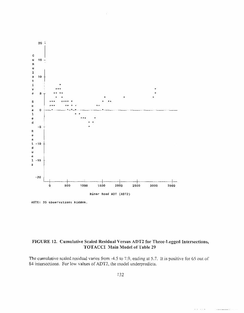
20
c
u 15
m
u
1
a 10t
i
v
,5
s
c
ao
1
e
d
-5
R
es
i -10
d
u
a
1 -15
s
20
,,,, ,
., ,, ,., * , *
,*, ,,. . , . ,.,,. ,, * , *.
—* ———— .—.-, ———-—.———●✎✿���✿✍���✎�����✍� ��✎✍���✎✎��
✌✎
✌✎✎ ✎
✌✎
✎
L-t__--_t-_--~_---__t---__-t___--_~_-__z~;_____i~;o 500 1000 1500 2000 2500
Minor Road ADT ~ADT2)
NOTE: 35 observations hidden.
FIGURE 12. Crsmuiative Scaled Residual Versus ADr2 for Tb ree-Legged Intersections,TOTACCI Main Model of Table 29
The cumulative scaled residual varies from -4,5 to 7.9, ending at 5.7. It is positive for 65 out of84 intersections. For low values of ~T2, the model underpredicts.
132

20
c
u 15
m
u
1
a 10
t
i
v
e5
s
c
aO
1
e
d
-5
R
e
s
i -10
d
u
a
1 -15
s
-20
. ●
● ✌
✌ ☛☛
☛ ✌☛
✌☛✎ ✌ ☛☛
�✌�☛☛✎✌✌☛✎�✎�☛�☛����� ✿✿✎ ��✎ ✿�✿✿�
☛ ☛✎ ☛✎☛
,“
**
, ,,
,
*
Median Width in feet (MEDW1OTH1)
NoTE: 44 observations hidden.
i ft = 0.305 m
FIGURE 13. Cumulative Scaled Residual Versus MEDWIDTH1 for Three-LeggedIntersections, TOTACCI Main Model of Table 29
The cumulative scaled residual varies from -7.2 to 6.2, ending at 5.7. It is positive for 32 out of84 intersections. On the eight intersections with median widths fmm 12 to 16 feet (3.7 to 4.9meters), the model underpredicts on average.
133

20t
Icu 15
m
u
1 *
alo- -* * ,
t ** **
i ** *.
v ***** ,*
e 5 -- *** ** **
,* * *.. **
s ●
c =
a 0 -- *
1 *
e *
d
-5 --Re
s
i -10
d
u
a
1 -15s t
I
No. of Oriveways (NODRWY1 )
NOTE: 45 observations hidden.
FIGU~ 14. Cumulative Scaled Residual Versus NODRVIYl for Three-LeggedIntersections, TOTACCI .Main Model of Table 29
The cumulative scaled residuai varies from -3.1 to 10.9, ending at 5.7. [t is positive for 69 out of84 intersections. men there are few driveways, the model tends to unde~redict crashes.
134

20
cu 15m
u
1
a 10
t
i
v
@5
sc
ao
1
e
d
-5R
e
s
i -$0
d
u
a
1 -15
s
-20
.
. ., ***
* ** .—*-*—* *_*_, _, .
*,, *.*,. * , ,.**
**.
~=~
Major Road AOT (AOT1)
MOTE: 36 observations hidden.
FIGU~ 15. Cumulative Scaled Residual Versus ADTI for Four-Legged Intersections,TOTACCI Main Model of Table 33
The cumulative scaled residual varies from -4.5 to 5.2, ending at -0.5. It is positive for 27 out of72 intersections.
135

20
cu 15m
u
1
a 30
t
i
v
e5
s
c
ao
1
e
d
-5
R
e
s
i -10
d
u
a
1 -15
s
-20
●
☛✎
✎✎ ☛☛☛ ✌
✿✎✿☛☛ ☛✎ �☛☛ ☛✿☛✿✎✿ ✎✿☛
● ☛☛☛ ☛ ☛☛
☛ ☛☛ ✌
☛☛✌☛☛✌
☛☛✌☛☛☛☛☛
✎☛
o 500 1000 3500 2060 2500
Minor Road AOT (ADT2)
NOTE: 24 observations hidden.
FIGUW 16. Cumulative Scaled Residual Versus ADT2 for Four-Legged Intersections,TOTACCI Main Model oflrable 33
The cumulative scaled residual vafies from -6.1 to 3.5, ending at -0.5. It is positive for 26 out of72 intersections. There is some indication of quadratic dependence on ADT2 or Log of ADT2 todescribe ove~rediction at low values of ADT2 and underprediction at higher values.
136

20
c“ ?5m
u
1a 10tiv@ 5
sc
a o
1
e
d
-5
R
@
s
i -lo
d
u
a
1 -15
s
-20 :
NOTE : 29
,.. *,* .,
—, .“ .*_*._*_
.,*
,* *
*.**
*., * ,,*
* .*, *.,%,
,.
,
~~
Peak Major Road Left Turn ~s (PK%LIEFT? )
observations hidden.
FIGU~ 17. Cumulative Scaled Residual Versus PKO/.LEFTl for Four-LeggedIntersections, TOTACCI Main Model of Table 33
The cumulative scaled residual varies horn -8.4 to 2.6, ending at -0.5. It is positive for 12 out of 72intersections. There is some indication ofoverprediction at lower turning percentages, followed byunde~rediction at somewhat higher turning percentages. A quadratic model addresses this mattel-in Variant 2 of Table 33, starting out with a smaller intercept and steeper slope, but with the slopebecoming smaller as PKOALEFTl increases.
137

20 +
c
u ?5
m
u
1
a 101
1
t’
i
v
e5. .
s ● **.*
c * . . . ****. * *
ao
1
e
d
-5
R
e
s
i -10
d
u
a
1 -15
s
-20
~*-**.—*–.—*—**.*—*——=–—*.. * .*
**
~~
Pdaior Roae ADT (ADTI )
NOTE: 11 observations hidden.
FIGU~ 18. Cumulative Scaled Residual Versus AIIT1 for Signalized Intersections,TOTACCI Main Model of Table 36
The cumulative scaled residual varies from -3.1 to 3.9, ending at -0.2. It is positive for31 OLIt of
49 intersections.
138

20
c
u 15
m
u
1
a iO
t
i
v
e5
s
c
ao
1
e
d
-5
R
e
s
i -10
d
u
a
1 -15
s
-20
**,, ** .* ****
_*_*_ *** *.—* *—.**———*, . . .**
**,
1 \ I~
o 5000 10000
Minor Road AOT (AOT2)
NOTE: 15 observations hidd@n.
FIGUW 19. Cumulative Scaled Residual Versus ADT2 for Signalized Intersections,TOTACCI Maiss Model of Table 36
The cumulative scaled residual varies from -5.4 to 4.2, ending at -0.2. It is positive for 29 out of49 intersections.
139

20
cu 15
m
u
1
a 10
t
i
v
e5
s
c
ao
1
e
d
-5
R
e
s
i -10
d
u
a
1 -15
s
-20
* ..** *● ☛ ✎ ✎ ✎ ☛ ✌✌ ☛ ✎
✿☛✿✌ ☛☛✿☛☛ ✎☛ ✎�☛� ☛� ☛✿
☛☛☛✎☛✌ ☛
● ☛ ✎✌ ✎☛☛
✎
I I I I I I~
0 10 20 30 40 50 60
Minor Road Left Turn % (FK%LEFT:?)
NOTE: 6 observations hidden.
FIGU~ 20. Cumulative Scaled Residual Versu!$ PKO/.LEFT2 for SignalizedIntersections, TOTACCI Main Model of Table 36
The cumulative scaled residual varies from -3.2 to 2.9, ending at -0.2. It is positive for 24 out of49 intersections.
140

20
c
u 15
m
u
1
a 10
t
i
v
e5
s
c
ao
1
e
d
-5
R
e
s
i -10
d
u
a
1 -15
s
-20
*** ,
**. , . ●
✎✌�☛ ☛☛☛ ☛��☛ —s——
* **.** , ● ,
**. *
**
*.
1 ! \ I I I~
o 1 2 3 4 5 6 7
Avg Grade Change1100 ft, All Legs (VEICOM)
NOTE: 14 observations hidden.
1 ft = 0.305 m
FIGUW 21. Cumulative Scaled Residual Versus VEICOM for Signalized Intersections,TOTACCI Main Model of?rable 36
The cumulative scaled residual varies from -4.6 to 3.2, ending at -0.2. It is positive for 19 OLItof49 intersections.
141

2C
c
u 15
m
u
1
a 10
tiv
e5
sc
ao1
e
d
-5
R
e
s
i -10
d
u
a
1 -15
s
-20
NOTE :
.,*.,** * . . . *
_., _*.*_*,_*_,_*_* —*——., **.
* ● ✎
✎☛
14 observations hidden.
.
~~
Peak Truck % (PK%TRUCK)
FIGU~ 22. Cumulative Scaled Residual Versus PK”ATllUCK for SignaltiedIntersections, TOTACCI Main Model of T~)ble 36
The cumulative scaled residual varies from -3.4 to 2.0, ending at -0.2. It is positive for 27 out of49 intersections.
142

Cumulative residuals for the TOTACCI Main Model of Table 36 (signalized intersections) areplotted in Figures 18 tkough 22. The explanatory variables are ADT1, ADT2, PROT_LT,
PK%LEFT2, VEICOM, and PKY.TRUCK. The vaiable PROT_Cr is not used in the residual1 The figures show what appear to be random walks with no particularmalysis since it is categorical.
systematic effects. Indeed, the fact that they stay relativel~’ close to zerO suggests that possiblyoverfitting is occurring.
Table 38 shows the range of values for the cumulative scaled residuals of all variables in theTOTACCI Main NIodels. The range is quite consistent with the square roots of the sample sizes.For PROT_LT, the sum of the scaled residuals over all signalized intersections without a protectedIefi turn is 0.45, so that tie signalized models slightly underpredict crashes on intersections withoutmajor road protected left turns. Since there are 28 signalized intersections without protected leftturns, the average scaled residual is 0.45/28 -0.016. The overall cumulative sum being -0.2, it fol-
TABLE 38. Cumulative Scaled Residuals Versus Increasing Value of IntersectionVariables, TOTACCI Main Models
84 three-leggedintersections(Table 29 MainModel)
m=9
72 four-leggedintersections(Table 33 MainModel) ~ = 8.5
49 signalizedintersections(Table 35 MainModel)
m=l
ADT 1 -7.2 to +10.2
ADT2 -4,5 to +7.9
MEDWIDTH1 -7.2 to +6.2
NODRWY 1 -3.1 to +10.9
ADT1 -4.5 to +5.2
ADT2 -6.1 to +3.5
PKVOLEFT1 -8.4 to +2.6
ADT 1 -3.1 t0+3.9
ADT2 -5.4 tO +4.2
PKYOLEFT2 -3.2 to +2.9
VEICOM -4.6 to +3.2
PKVOTRUCK -3.4 to +2.0
PROT_LT ~-0.2, +0.451
143

lows that the sum of the scaled residuals on the intersections where major road protected left turnsme present is -0.6S, for an average on the latter intersections of-0.6S/21 = -0.031. Thus, the modelslightly overpredicts on the intersections that have major mad protected left turns.
In summary,
. The three-legged Main Model for TOTACCI mig~t be improved by partitioning theintersection variables into smaller ran ges and developing models for each range.
. The four-legged Main Model for TOTACCI might be improved by inclLldlLlg qLLadraticdependence on ADT2 or the log of ADT2 audlor PKYoLEFTl.
. The signalized Main Model for TOTACCI has well-behaved residuals, possibly an indicationof overfitting.
In view of the relatively small sample sizes, the models all behave reasonably well.
A residual analysis was not done for the TOTACC models, although it is believed that it wouldyield similar results.
I44

6. CONCLUSIONS
In this chapter, we exhibit the Main Models for TOTACC and TOTACCI again. Then, we use thesemodels and the log-likelihood R* to decompose the variation in crashes into proportions due todifferent variables. We also develop Accident Reduction Factors for the models. Finally, we reviewand summarize ideas in this study.
THE MAIN MODELS
Three-Legged Intersections
1. Three-le~sed rural intersections of a four-lane maior road with stou-controlled two-lane minorroad. TOTACC Main Model (Table 28)
Negative Binomial Model with K = 0.389
j= NUMBER OF YEARS x (AD T1)’”48 x (AD~2)0’2s2 x e~p(-~2.22~)x exp(-O.0546XMED WZDTHI + 0.0391 xNODR WY1)
where the variables are:
~ = predicted mean number of crashes within 250 feet (76 meters) of the intersectioncenter
WMBER OF YEARS
~T 1 = average two-way major road traffic in vehicles per day
ADT2 = average two-way minor road traffic in vehicles per day
MEDWIDTH1 = the major road median width in feet
NODRWY1 = the number of residential and commercial driveways on the major roadwithin 250 feet (76 meters) of the intersection center.
NOTE: A - version of this model is obtained by repla:ing - 0.0546 xMEDWIDTH1 abovewith -0.179 x MEDWIDTH 1., w!nere MED WIDTH 1. = the major road median width in meters.
145

II. Three-lez~ed rural intersections of a four-lane maior road with sto~-controlled two-lane minorroad. TOTACCI Main Model (Table 29)
Negative Binomial Model with K = 0.512
y= NUMBER OF YEARS x (ADTI)1433 x (ADT2)”’269 x exp( -15.466)X exp(-0.@612 XMEDW1DTHl + 0.0560 xNODRWYI)
where the variables are:
~ = predicted mean number of intersection-related crashes within 250 feet (76 meters)of the intersection center
NMBER OF YEARS
ADTI = average two-way major road traffic in vehicles per day
ADT2 = average two-way minor road traffic in vehicles per day
MEDWIDTH1 = the major road median width in feet
NODRWYI = the number of residential and commercial driveways on the major roadwithin 250 feet (76 meters) of the int(:rsection center.
NOTE: A X version of this model is obtained by replacing - 0.0612xMEDWIDTH1 abovewith -0.201 x MEDWIDTH1., where MEDWIDTHln, = the major road median width in meters.
146

Four-Legged Intersections
I. Four-1 egged rural intersections of a four-lane maior road with sto~-controlled two-lane ]minorroads. TOTACC Main Model (Table 32)
Negative Binomial Model with K = 0.458
0850 x (~~TZ)o.329 X exp( –9.463)y= NUMBER OF YEARS x (ADTI)x exp(O.l lOxPKO/oLEFTl – 0.484 xLTI,NIS)
where the variables are:
~ = predicted mean number of crashes within 250 feet (76 meters) of the intersectioncenter
~MBER OF YEARS
ADT1 = average two-way major road traffic in vehicles per day
~T2 = average two-way minor road traffic in vehicles per day
PKYoLEFT 1 = the percentage of incoming major mad traffic during peak hours that turnsleft
LTLNl S = Oif the major road has no left-turn lane, 1 if the major road has at least oneleft-turn lane.

II. Four-lezzed rural intersections of a four-lane maior road with stou-controlled two-lane minor
roads. TOTACCI Main Model (Table 33)
Negative Binomial Model with K = 0.710
f= NUMBER OF YEARS x (AD Tl)”’930 x (AD T2)”’354 x ex~(-l~.~ 10)x exp[0.149xPK”/. LEFTI)
where the variables are:
f= predicted mean number of intersection-related crashes within 250 feet (76 meters)of the intersection center
WMBER OF YEARS
ADT1 = average two-way major road traffic in vehicles per day
ADT2 = average two-way minor road traffic in vehicles per day
PKOALEFTl = the percentage of all incoming major road traffic during peak hours thattt)ms left.
148

Signalized Intersections
1, Siqalized four-leqzed rural intersections oftwo-lane roads. TOTACC .Main Model (Table
u
Negative Binomial Model with K = 0.116
0620 ~ (ADTJ)03y5 x exp(-6.9~4)~= NUMBER OF YEARS x (ADT1)x exp(–0.0142 xPK0/0LEFT2 + 0.0315 xPK”/. Tl8UCQx exp(–O.675xPR0T_LT + 0.130 xVE1CQM)
where the variables are:
$ = ~n~y mean number of crashes within 250 feet (76 meters) of the intersection
mBER OF YEARS
AOTI = average two-way major road traffic in vehicles per day
~T2 = average two-way minor road traffic in vehicles per day
PKY0LEFT2 = the percentage of all incoming minor road traffic during peak hours thatturns left
PKY.TRUCK = the percentage of all incoming traffic during ]?eak hours that consists oftrucks
PROT_LT = Oif the major road has no protected left turn, 1 if the major road has at leastone protected Iefi turn
VEICOM = (1/2) (VEI-1 + VEI-2)
VEI-1 = the sum of absolute percent grade change per 100 feet (30.5 meters) for eachvertical curve along the m~ or road, any portion of which is within 800 feet (244meters) of the intersection center, divided l~y the number of such curves
VEI-2 = the sum of absolute percent grade change per 100 feet (30.5 meters) for eachvertical curve along the minor mad, any portion of whic]l is within 800 feet (244
meters) of the intersection center, divided by the number of such curves.
NOTE: A * version of this model is obtained by replacing 0. 130xVEICOM above with
149
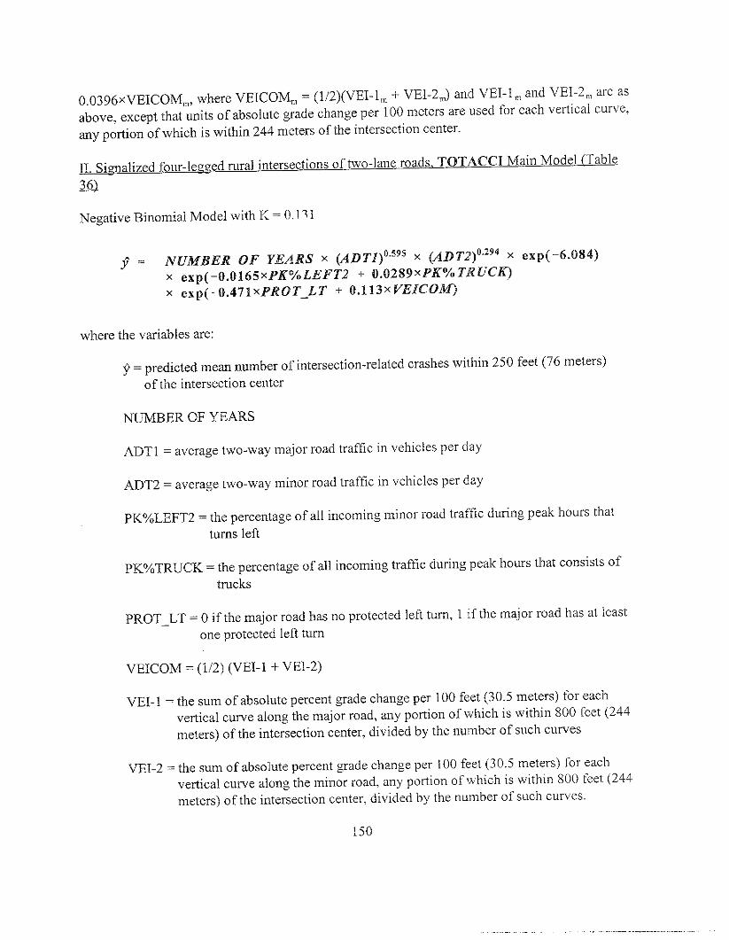
0.0396 xVEICOM~, where VEICOM~ = (1/2) (VEI-1~ + VE1-24 and VEI-I ~ and VEI-2”, are asabove, except that units of absolute grade change per 100 meters are used for each vertical curve,
my pofiion of which is within 244 meters of the inters ectiorl center.
11.Signalized four-leqq ed rural intersections oftwo-lane roads. TOTACCI Main Model (Table
m
Negative Binomial Model with 1<= 0.1 ~1
~= NUMBER OF YEARS x (AD Tl)O’59s ‘( (AD T~)O’294x ‘XP( ‘~.0g4)x exp(–0.0165 xPK0/0LEFT2 + 0.0289 :~PKO/oTRuc~x exp(–O.471XPR0T_LT + 0.113x VEICOM)
where the variables are:
~= predicted mean number of intersection-related crashes within 250 feet (76 meters)of the intersection center
~MBER OF YEARS
ADT 1 = average two-way maj or road traffic in vehicles per day
ADT2 = average two-way minor road traffic in vehicles per day
pKYOLEFT2 = the percentage of all incoming minor road traffic during peak hours that
turns left
PKYoTRUCK = the percentage of all incoming traffic during peak hours that consists oftrucks
PROT_LT = O if the major road has no protected left turn, 1 if the maj or road has at leastone protected left turn
VEICOM = (1/2) (VEI-1 + VEI-2)
VEI-1 = the sum of absolute percent grade change per 100 feet (30.5 meters) for eachvertical cuwe along the major road, any pcrtion of which is within 800 feet (244meters) of the intersection center, divided by the number of such curves
VEI-2 = the sum of absolute percent grade change per 100 feet (30.5 meters) for eachvertical curve along the minor mad, any portion of which is within 800 feet (244.meters) of the intersection center, divided ‘by the number of such curves.
150
. ..—

NOTE: A - version of this model is obtained by replacing O.113xVEICOM above with0.0344 xVEICOM~, where VEICOM. = (1/2) (VEI-f”, + VEI-2~ and VEI-I ~ and VE1-2n, are asabove, except that units of absoiute grade change per 100 meters are used for each vertical curve,any portion of which is within 244 meters of the intersection center.
EXPLANATORY VALUE OF MAIN MODELS
A customary way to measure the explmatory value of variables in a model is to note the incrementto a goodness-of-fit measure as each variable is added to the model. For Poisson and negativebinomial models, as FridstrOm et al. (1995) have observed, there is inherent randomness in the modelthat needs no explanation. With respect to the Iog-likelihood R-squared measure proposed byFridstrOm et al., negative binomial randomness is represented by 1- P; where P; is as in equation(5.5) of Chapter 5. The contribution of other factors is represented by: (i) R; for the first variablewhen a model with that variable present is used, and (ii) the increment in R; for each additionalvariable as it is successively added to the model. Recall tht; definition of R~ in eqoation (5.4) ofChapter 5. Finally, the unexplained portion of variation is P;, - R~~where R~Jis the R-squal.ed \alueobtained when all variables are present.
Tables 39,40, and 41 and Figures 23,24, and 25 decompose the variation according to this methodfor each of the Main Models.
TABLE 39. Explanation of Variation in Total Crashes by (;roups of Covariates,Main Three-Legged Intersection .Modens
3-Legged Log-Likelihood ~
Intersection Coefficient ofMain Models (Tables 28 and 29) Determination (%)
TOTACC TOTACCI
Randomness 44.11 46.26 ~
Exposure (ADT1, ADT2) 18,21 17,31
Design (MEDWIDTH 1, NODRWY1 ) 4.26 5.02
Unexplained 33.42 31.41
TOTAL 100.00 100.00
151

100:
80
20
E Unexplained
Design—..Kj: Exposure
Randomness
oTOTACC TOTACCI
RIGURE 23. Explanation of Variation of TOTACC and TOTACCIby Groups of Covariates, Main Negative Binomial Models for Tl]ree-Legged Intersections,
Log-Likelihood R-$qua)red
For the three-legged intersections, ADT explains 17 to 18% of the variation, while .MEDWIDTH 1and NODRW1 explain another 4 to 5Vo. For the four-leg2ed intersections, ~T explains 8 to 100/0of the variation, while major road left-turn percentage andlor the presence of a major road left-turnexplains another 5‘A.
In shq contrast, for the signalized intersections, ADT by itself explains a negligible percentage ofcrashes. Turning and truck percentages explain 1 to 3°/0and the design variables PROT_LT andVEICOM explain between 6 and 13Y0,depending on the model. As FridstrOm et al. (1995, p. 11)
point out, the explanatory vaIue of a variable may well be affected by the order in which variablesare added. This is amply demonstrated by Table 41 and Figure 25. A more cautious interpretation!of Table 41 is that in the case of the TOTACC model. 0.34 + 1.46 + 12.99 = 14.790/. of the variationis explained by the six intersection variables, and in the case of the TOTACCI model, 0.00 + 3.2;’
1j2

+ 6.16 = 9.43 “Aof the variation is explained by the six intersection variables. Furthermore, the
proportion of the explanato~ power that is attributable to the individual variables is uncertain, ADTaIone does not explain much.
TABLE 40. Explanation of Variation in Total Crashes by Groups of Covariates,Main Four-Legged Intersection .Models
4-Legged Log-LikelihoodIntersection Coefficient of
Main Models (Tables 32 and 33) Determination (Yo)
TOTACC TOTACCI
Randomness 41.42 42.85
Exposure (ADT1, ADT2) 10.79 8.14
PKVOLEFTI 2.55 5.20
LTLNI S 2.89
Unexplained 42.35 43.81
TOTAL 100.00 100.00
TABLE 41. Explanation of Variation in TotaICra.shes by Groups of Covariates,Main Signalized Intersection Models
Signalized Log-LikelihoodIntersection Coefficient of
Main Models (Tables 35 and 36) i Determination ~A)
TOTACC TOTACCI
Randomness 37.38 41.46
Exposure (ADT1, ADT2) 0.34 0.00
PKYOLEFT2, PKYOTRUCK 1 1.46 3.2J
VEICOM,PROT_LT 12.99 6.16
Unexplained 47.83 49.11
TOTAL 100.00 100.00
153
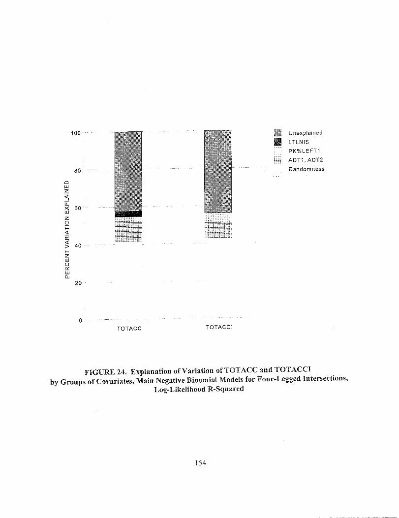
TOTACC TOTACC’i
Unexplained
LTLNIS
PK”ALEFTl
AOTI, ADT2
Randomness
FIGU= 24. Explanation of Variation of TOTACCand TOTACCI
by Groups of Covariates, Main Negative Binomial Mo(iels for Four-Legged Intersections,Log-Likelihood R-Squalred
154

100
TOTACC TOTACCI
Unexplained
VEICOM, PROT_LT
PKYOLEFT2, PK”ATRUCK
ADTI, ADT2
Randomness
FIGURE 25. Explanation of Variation of TOTACC and TOTACCIby Groups of Covariates, Main Negative Binomial Models for Signalized Intersections,
Log-Likelihood R-Squared
ACCIDENT WDUCTION FACTORS
The Main Models yield the Accident Reduction Factors shown in Table 42. Recall hat the Accidenl:Reduction Factor is the percentage decrease in mean pre[iicted crash count when a variable isincreased by one unit, all other variables being held fixed. A negative value signifies that crashesincrease by that percentage when the variable is increased by one unit.
For the three-legged intersections, the TOTACC and TOTA.CCI models yield similar results. It ija ctiosity that the number of driveways is more significant :forintersection-related crashes than for
155

all crashes, given that the former attempts to exclude driveway crashes and the latter does not.
TABLE 42. Accident Reduction Factors for the Main Models
3-Legged intersections
TOTACC Main Model TOTACCI lMain Model
Table 28 Table 29
MEDWDTH1 5.3% 6.6%
NODRWY 1 -4,0Y0 -5.7Y0
4-Legged intersections
TOTACC Main Model TOTACCI Main ModelTable 32 Table 33
PK%LEFT1 -1 1.6% -16.1°A
LTLNIS 38.470
Signalized intersections
TOTACC Main Model TOTACC1 Main ,Model
Table 35 Table 36
PKYOLEFT2 1.4% 1.6%
PK%TRUCK -3.2Y0 -2.9Y0
PROT_LT 49.l”h 37.5”A
VEICOM -13.9Y0 -11.9”A
Note: Negative Accident Reduction Factors signify an increase in accidents.
For the four-le~~ed intersections, the TOTACC model declares that the Presence of one or more left----turn lanes reduces crashes by 38.4°/0. LTLNrl S had a high P-value (0.3222) when applied tc,TOTACCI andappears only inthe Variant 1 and Variant 3modelsof Table 33. In the Variant 1model, its Accident Reduction Factor is25.10A, \vhilethat of PK0/oLEFTl is-15.3°/0. The number25.1 Y. is not as large as 38.4%, but is still quite substantial.
Variables in the signalized intersection models show simil.ar Accident Reduction Factors as am:passes from TOTACC to TOTACCI. Only PROT_LT shows a dranlatic decreases in i~effectivenessby going from 49.1°A to 37.5°/0. The two regression coefficients fOr PROT_LT on
156

which these estimates are based have overlapping confidence intervals so that the difference between49.l% and 37.5% may be ilhrsory.
The effect of PKOALEFTl in different models is of some interest. Consider TOTACC models forall three classes of intersections containing this variable, namely, the Variant Model in Table 28, theMain Model in Table 32, and Variant 2 in Table 35. The respective Accident Reduction Factors are-5.6Y0, -1 1.60A, and -2.20A. For each l-percent increase in left turns from the major road, crashesincrease by 5.6°/0, 11.60/., and 2.20/0 at three-leggec~, four-legged, :.!>d slgnahzeci intel-sc.,c..~,respectively. A superficial justification of the relative sizes of these numbers runs as fo[lows: at thefou-legged intersections, a driver turning left from the major road has to worry about t~affic fromboth minor legs; at a three-legged intersection, the driver has to worn] about traffic from only oneminor leg; and at a signalized intersection, the driver has to worry about neither minor leg (as longas the signal is green). Even if minor road ADT is low, the presence of minor legs requires somedivision of attention.
SUMMARY
The Main Models presented at the beginning of this chapter are the primary product of this study.There are six such models, one for each of the three intersection classes and for each oftbe two crashtypes TOTACC and TOTACCI. Because our sample sizes were small, we judged it expedient to useall observations for model development and reserve none for prediction, so no efforts have beenmade to test the predictive powers of the models. The models are, however, reasonably stable:potentially influential observations were removed and the models retained similar coefficients andP-values.
With regard to the two crash types TOTACC and TOTACCI, we do not make a selection. Themodels for each are reasonably consistent with one another, the variables are mostly the same, and
the regression coefficients are similar. For the three-legged and four-legged intersections, theexception is that as one passes from TOTACC to TOTACCI, the intercept gets smaller and thecoefficient of the log of ADT 1 gets larger. TOTACC1 is more sensitive to major road ADT than.TOTACC. On the signalized intersections, in the same transition, the intercept gets larger and thecoefficients of the logs of both major and minor ADT get smaller. TOTACCI is less sensitive tc~T than TOTACC. These trends are systematic, but not too much weight should be put on tbelr.since the standard errors of the coefficients do not preclude the possibility thdt the true coefficientsare equal (but there must be a net adjustment downward somewhere since TOTACCI < TOTACC).
Both the TOTACC models and the TOTACC1 models are equally serviceable. A decision on whichto use should be based on what they will be used for and how overlapping models will be assembledto represent all crashes. of some importance is agreement among interested parties as to what an
intersection-related crash is. Desirable properties include simplicity, i.e., an understandabledefinition, and practicsrlity, i.e., one that can be used to extract data from existing or soon-to-existdata bases, The treatment of driveway crashes, run-off-road crashes, and minor road crashes that
157

are not intersection-related should be addressed. Also, a decision is needed about whether the samecriteria can be used to define intersection-related crashes for di fferent kinds of intersections: oneswith two-lane versus four-lane major roads, ones with or without signals, and ones in urban versusrural environments. The BMI criteria discussed at the beginning of Chapter 4 were used in thisstudy, but they had a limited purpose and scope and their overall applicability should be reassessed.
The same considerations apply to INJACC versus INJACC1 models. Their differences andsimilarities mirror those betweer, the TOTACC and TOTACCI modeIs.
A separate issue is whether injury crash models am needed. A reaso:a not to develop them is thatit may suffice to apply a percentage to TOTACC or to TOT,4CCI in order to estimate INJACC or~JACCI. Tables 9 and 10 in Chapter 4 suggest that injury crashes as a proportion of all accidents
VW at Ieast by State and by intersection class. However, the State variable in this study seemed tohave no independent influence, and this is a significant finding of our study. Our evidence suggeststhat serious crashes at three-legged and four-legged intersections are not distributed in the sameproportion relative to all crashes at different intersections. Although we do not identify MainModels for INJACC or fNJACCI, we do develop ~JACC and IhrJ.4CCI models. It is worthwhileto compare such models with TOTACC/TOTACCI models. For the three-legged intersections, theangle variable HAU assumes prominence and median width loses importance. For the four-leggedintersections, minor road posted speed gains influence and channelization loses influence. On theother hand, INJACCl~JACCI models for signalized intersections are similar to theTOTACC/TOTACCI models. Since injury crashes are of greater concern to society and are betterreported, contrasts between models for injury crashes and all crashes deserve attention.
We also argue that the variant models shown in the tables of Chapter 5 are worthy of attention.When P-values are large, it is not possible to confirm that the true regression coefficient is non-zero.Thus, an estimated regression coefficient of 0.3 with an estimated standard error of 0.3 could wellbe a fluctuation for a variable whose tme coefficient is zero, the variable thus having no bearing on.crash experience. On the other hand, the fluctuation could run in the opposite direction and the trueregression coefficient might be 0,6. The estimated coefficient 0.3 summarizes the sample at hand.accurately (as does its standard error 0.3) and may be regarded as a point estimate for the trueregression coefficient. It is the single best guess as to what that coefficient is. If its standard erroris large, there is the possibility that this coefficient might be zero, but the true answer might also bt~twice as large. If engineering judgment supports the sign and rough magnitude of a regressioncoefficient, som,e Iatitade is in order.
Variant 1 in Table 33 “issuch a case. The variable LTLN 1S, representing the existence of a Ieft-tumlane, has an estimated coefficient of -0.2891 with an estimated standard error of 0.2920 (and a P-value of O.3222) in a TOTACCI model. This variable is significant in the TOTACC model and issignificant in another TOTACCI model, Variant 3 in Table 33.
All of the models are, of course, subject to caveats. The definitions of TOTACC and TOTACCI areimperfect. California and Michigan assign crashes to an intersection out to different distances along
158

the minor mad. TOTACCI in CaIifomia, but not in Michigan,, may contain some driveway crasheswhere a car is entering a driveway. Alignments, sight distances, grades, and median widths aresubject to measurement errors, and a~y and all variables may have changed from the time period1993-1995 to the time of the field work (1997-1998).
Of special concern, since they are so prominent in the models, are the peak-hour traffic data. Wehave referred to some of them as turning percentages or peak turning percentages. But they are in
fact merely a sample of peak-hour turning percentages collected during a po}tion of peak hours ona particular day in 1997-1998 and are averaged between morning and evening. They can be regardedas crude estimates of the true average peak-hour turning percentages or truck percentages during1993-1995. But even the variable one is trying to estimate is somewhat suspect. A peak hour canbe defined by a clock definition or by actual experience along a highway. The latter seems morepertinent to crash experience, b~t the former is presumably closer to what we have.
Yet another issue, one that has not been addressed in this study, is how peak-hour turningpercentages should relate to ADT. If one were dealing with true mean turning percentage, it wouldseem that a model form would be required that yields zero crashes when all turning percentages arezero. As a practical matter, if, for example, major road turning percentages are zero, then we canusually assume that there is zero minor road traffic. Relationships can Ibebuilt into the model formto ensure that this happens. Since we are dealing with peak-hour turning percentages rather than truemean 24-hour turning percentages, it is possible in principle that the former could be zero withoutthe latter being zero and that the latter could adjust itself to be compatible with almost any observedvalues of ADT2 or ADT1. Rather than address these thorny issues, we have taken an empirical pointof view and allowed interrelated vtiables, such as the log of ADT 1, the log of ADT2, PKO/OLEFT1,pK0ALEFT2, ~d PKVOTHRU2, to appear in generalized linear expressions without regard to their
hypothetical mutual constraints.
Indeed, especially in the case of the signalized intersections where ADT behaves somewhatpeculiarly when other variables are missing, as confirmed in Table 26 and Figure 9 as well as Table4 I and Figure 25, new model forms should be explored that might better describe the data. Thelimited data in this study suggest that at signalized intersections, some measure of turning percentage(e.g., PROT_LT, PK%LEFT1, PK%LEFT2) should be adjoined to major and minor mad ADT asthe primary intersection variables. It would also be desirable if new model forms retained someaffinity with existing forms that have been adequate for other classes.
One caveat for all of the models is that some variables have rather wide ranges, e.g., NODRWY1,PKY,LEFT2, PKYOTR. The coefficients assigned to these variables represent their behavior aslinear. Over such wide ranges, piecewise linear or quadratic dependencies might be moreappropriate. Ezra Hauer has suggested that model forms where the mean number of crashes dependson major mad ADT through expressions of the form (ADT 1~xexp(-bxADTl ) or exp(ax (Log ofADT1) bxADTl ), with a and b positive, should be explored. Figures 5 and 9, for three-legged andsignalized intersections, respectively, suggest such a possibility. A similar form could be appliedto minor road ADT. More elaborate fomls could also be considered that allow crash frequency tc

rise to a maximum as ADT 1 increases, with the value of A.DT i at which the maximum occursdepending on ADT2.
We recapitulate the main points below:
.
.
.
.
The data in this study have shortcomings. These include relatively small sample sizes, peakturning percentages and truck percentages measured by samples not contemporary with thecrash data, and the difficulty of meast!~ing and defining crash and intersection variables
In addition to the six Main Models, alternate models cleserve consideration. These includevariants given in the tables using other variables, the Flow Models in Chapter 5, models thatrestrict the range of certain inputs (piecewise linear) or allow quadrsstic dependencies, andmodel forms suggested by Hauer.
Major road ADT plays a lesser role as one passes from three-legged to four-legged tosignalized intersections, with turning percentage measures becoming more important, andunexplained crash frequency variation increasing (Figures 23, 24, and 25).
The six Main Models adequately summarize the data in this study, with the choice of a crashvariable TOTACC (all crashes within 250 feet (76 meters)) or TOTACC I (all intersection-related crashes within 250 feet (76 meters)) to be detcmined by other criteria.
160

APPENDIX. DATA FROM PILOT STUDY PHASE OF DP,TA COLLECTION
During the pilot study phase of data collection for this report, in March and May 1997, plates wereused to collect traffic data on minor legs of signalized intersections in Michigan and radar guns wereused to measure operating speeds on all legs of intersectiolts in both California and Michigan.Figures A-1, A-2, and A-3 exhibit some relationships obtained from these data. In addition an area-of-influence study was done on a few selected intersections to judge whether crashes near theintersectio~. were intersection-related. Figure A-<!shows the findings for one such intersection.
Figure A-1 is a graph of posted speed versus observed opera:ing speed at signalized intersections.Operating speeds were determined by radar guns aimed along the road toward the intersection duringdaytime hours out of sight of the intersection or far enough away so that drivers typically bad notbegun to slow. The graph shows that many drivers exceed the posted speed limit, but that the excesstends to be less at low and high speeds and greater at intermediate speeds.
Figure A-2 is a graph of daytime speeds versus 24-hour speeds along minor legs approachingMichigan signalized intersections. Daytime speeds were messsured by radar guns, and 24-hourspeeds by HISTAWN-METRICS plate counts. It is appartmt that the 24-hour speeds are Iowel-,although some of the extreme cases may represent miscalibrat ion of the radar guns andor the pIates.
Figure A-3 shows that truck percentage in off-hours tends to be higher than in peak hours. At theend of Chapter 4, it is noted that a.m. truck percentage is higher than p.m. truck percentage as well,and that Miaou et al. (1988) have called for studies of truck percentage by time-of-day. Betweena.m. and p.m., a rough reversal of movements was found for all traffic (e.g., soutl~boandpredominance in a.m., northbound in p.m.) although variances were large. Truck percentage is asmall portion of the total during peak hours, and may be larger in off-hours, chiefly becausenoncommercial traffic lessens.
A few intersections in this study were examined in detail, in an effort to analyze the area of influenceof an intersection, i.e., how far out from the intersection center intersection-related crashes are likelyto be found. For this purpose, all crashes within 500 feet (152 meters) of the intersection center wereexamined. Figure A-4 shows crash locations for one such intersection. A distance of 250 feet (76meters) from the intersection center includes most intersection-related crashes, misses a few, andpicks up a few that are not intersection-related. Crashes that are not intersection-related are morelikely to be found on the outward bound lanes from the intersection center. One State high~vayengineer reported intersection-related crashes that occurred on roads that did not pass through theintersection. During heavy traffic, a driver turning onto an intersection leg from a side road issometimes involved in a crash related to the main intersection.
161

POSTED SPEED VERSUS OPERATING SPEED
24 Signalized Intersections, Pilot Studies, CA & Ml, 199760 . . . .
‘--:-E*””””“Q
’25
2030 35
_—
. . . .
5040 4,5
Posted Speed (mph)
posted speed
median operating speed
85th percentile operating speed
Operating speeds were measured during daytime hoursby radar guns well away fiOm the intersection1 mph= l.61 kmh
55
FIGURE A-1. Posted Speed Versus operating Speed
162

Daytime Speed vs. 2A-bIour Sp~ed
?9 Signalized Intersections, Minor Le9~, Michigan, May lgg7
55
Daytime speeds were measured by radar guns.24-hour speeds were measured by HIS’r~-METRICS plate counts.1 mph= 1.61 km/h
FIGU~ A-2. Daytime Speed Versus 24-Hour Speed
163

PEAK TRUCK PERCENTAGE VERSUS 24-HOUR TRUCK PERCENTAGE
Peak Truck Percentages were measured by daytime manual count.24-hour Truck Percentages were measured by HIST~-MET~CS platecounts.
FIGU~ A-3. Peak Truck Percentage Versus 24-Hmsr Truck Percentage
164

cAState Route 28intersects Fox Street inplacer County. ThisintersectiOn (cnty_fie =’’0302831~’, milepost= 10.025 )has minor leg
stop control, isofthe Ttype, four-laIle bytwo-lane, with arightangle> andnolnedians on any leg. Theintersection isinrollingte~ainwith aHAZWT equal to2. The longitudinal sight distance for leg 1 is80~feet (244 meters). Although theintersection is defined as``meal,'' itisinthe Lake Tahoe resofiarea with 12coI~ercial driveways alOng legs 1 ~d2within+250 feet (76meters) of the intersection
center. This isahigh-crash intersection with 17craslles occ~l~ing within +500feet(152 llleters) oftbeintersection center during the years]993-1995. Onthebasis ofreview of~lSIS files, thecrashes with Ilunlbers inparentheses were deelned nottobe intersection-related.
FOXSt. (Leg 3)
‘Route2x(Leg1) .ll~ E.Roue8Leg~(5) (1)
6.12.13 (17),,4,7, 15 0:
8 9 142,3, 11
!@
(16)
500 400 250 150 100 50 0 50 100 ljO 250
Crash locations are numbered; those with parenthesesare not thought to be intersection-related.1 ft = 0.305 meters
400 500 ft
FIGUREA -4. Crtisl] l.ocations and ReIationsllips ata Three-I, egged Intersection
165

REFERENCES
American Association of State Highway and Transportation Officials, A PolicY on Geometric Designof Highways and Intersections, Washington, D. C., 1994.
J.G. Bared and H. Lure, “Safety Evaluation of Intersection Design Elements (Pilot Study),’”
Transpofiation Research Board Conference Presentation, Washington, D. C., 1992.
K.M. Bauer and D. Harwood, Statistical Models of At-Grade Intersection Accidents, Report No.FHWA-~-96- 125, Federal Highway Administration, McLean, Vs., 1996.
D. Blower, K.L. Campbell, and P.E. Green, “Accident Rates for Heavy Truck-Tractors in Michigan,”Accident Analysis and Prevention 25 (3): 307-321, 1993.
J,A. Bonneson and P.T, McCoy, “Estimationo fSafetya tTvvo-WayS top-Controlled Intersections
on Rural Highways? Transportation Research Record 1401.: 83-89, 1993.
U. Btide and J. Larsson, ``Models for Predicting Accidents at Junctions Where Pedestrians andCyclists Are Involved: How Well Do They Fit?’ Accident Az!alysis and Prevention 25 (5): 499-509,
1993.
N.A, David and JR. Norman, Motor Vehicle Accidents in Relation to Geomet~ic and TrafficFeatures of Highway Intersections, Volume II- Research Report, RePoti No. FHWA-~-76-129,Federal Highway Administration md National Highway Traffic Safety Administration, Washington,D. C., 1975.
C. Dean and J.F. Lawless, “Tests for Detecting Overdispersion in Poisson Regression Models,”Journal of the American Statistical Association 84 (406): 467-472, 1989.
R. Elvik, “Mets-Analysis of Evaluations of Public Lighting as Accident Countermeasures,”Transportation Research Record 1485: 112-123,1995.
L. FridstrOm, J. Ifver, S. Ingebrigtsen, R. Kulmala, and L.K. Thomsen, “Measuring the Contribution
of Randomness, Exposure, Weather, and Daylight to the Variation in Road Accident Counts,’”Accident Analysis and Prevention 27(1): 1-20,1995.
N.J. Garberand R. Srinivasan, ’’Risk Assessment of Elderly Drivers at Intersections: Statistic!Modeling:’ Transportation Research Record 1325:17-22, 1991.
A.S. Hakkert and D. iMahalel, “Estimating the Number of Accidents at Intersections From afiowledge of the Traffic Flows on the Approaches, “AccidentA nalysisa ndPreventio~l 10:69-79,1978.
167
J.T. Harma, T.E. Flynn, and W.L. Tyler, “Characteristics of Intersection Accidents in Rural
Municipalities, '' Transportation Research Record 6Ol:79-Z{2, 1976.
D.W. Harwood, M.T. Pietrucha, M.D. Woolridge, R.E. Brydia, and K. Fitzpatrick, .Medianintersection Design, N'ational Cooperative Highway Research Program Report 375, TransportationResearch Board, National Research Council, NationaI AcadelnyPress, Washington, D.C., 1995.
E. Hauer, Obsemational Be~ore-A~e~Studies i~Road Sa~ely, PerSaon Press, 0x ford, U.K., 1997.
E. Hauer and A.S. Hakkert, “Extent smd Some Implications of Incomplete .4ccident Reporti n:,”Transportation Research Record l185: 1-10,1988.
E. Hauer, J.C.N. Ng, and J. Lovell, “Estimation of Safety at Signalized Intersections,”Transportation Research Record 1185:48-61, 1988.
E. Hauer, E. Pagitsas, and B.T. Shin, “Estimationo fTurningF lows From Automatic Counts,”Transportation Research Record 795: 1-7,1981.
E. Hauer and B. Persaud, Safety Analysis of Roadway Geometty and Ancillary Features,Transportation Association of Canada, Ottawa, 1996.
E. Hauer, D. Te~, and M. S. Griffith, ``Effect of Resurfacitl,g on Safety of Two-Lane Rtlral Roadsin New York State, '' Transportation Rese~~rchRecorc[l467; 3fl-37, 1994.
H. C. Jokschand L.P. Kost~iuk,lModeling Iittersection Crash Cozl?7tsancl Traf$c Volarne, ReportNo. FHWA-~-98-096, Federal Highway Administration, iMcLean,TJa., 1998.
G.F. King and R.B. Goldblatt, “Relationship of Accident Patterns to Type of Intersection Control,”Transportation Research Record 540: L-12,1975.
M.W. Knuiman, F.M. Council, and D.W. Reinfurt, “Association of Median Width and HighwayAccident Rates,” Transportation Research Record 1401:70-82, 1993.
S.R. Kuciembaand J.A. Cirillo, Safety Effectiveness of Hi!ghway Design Features, Voluwie V-Intersections, Report No. FHWA-RD-91 -048, Federal Highway Administration, Washington, D.C.,1992.
R. Kulmala, Safety at Three- and Four-Arm Junctions: Development and Application of AccidentPrediction Models, VTTPublication 233, Technical Research Centreof Finland, Espoo, 199j.
M. Y.-K. Lau and A.D. May, Accident Prediction &[odel L~evelopment: Signalize[l lnterseclion.~,Research Repofl UCB-lTS-R-88-7, Institute of Transportation Studies, University of California.Berkeley, Ca., 1988.
168

H. Lumand J. Reagm, Interactive .Vighway Safety Design Model: Accident Predictive Moclule,FHWA Drafi 8-22-94.
G. Maycock and R.D. Hall, Accjdents at 4-Arm Raundabou!ts, Laboratory Report I I20, Transportand Road Research Laboratory, Department of Transport, Crowthome, Berkshire, United Kingdom,1984.
P.T. McCoy, W.J. Hoppe, and D.V. Dvorak, “Benefit-Cost Evaluation of Left-Turn Lanes onUncontrolled Approaches of Rural Intersections (Abridgement),” Tra~sportatiot~ Researcjl Record1025:40-43, 1985.
P.T. McCoy, E.J. Tripi, and J.A. Bonneson, Guiclelinesfor Realignment of Skewed Intersection..~,Nebraska Depatiment of Roads Research Project Number R.ESl (0099) P471, 1994.
J.W. McDonald, “Relation Between Number of Accidents and Traffic Volume at Di\ided- HighwayInters ections/ Highway Research Board Bulletin 74, Traf@c-Accide!t tStudies, pp.7-17, Nationa]Academy of Sciences, National Research Cotlncil, Washington, D. C., 1953.
H.W. McGee, W.E. Hughes, and K. Daily, Effect of Highway St~~ndards on Safety, National
Cooperative Highway Research Program Report 374, Transportation Research Board, NationalResearch Council, National Academy Press, Washington, DC., 1995.
S.-P. Miaou, “The Relationship Between Truck Accidents and Geometric Design of Road Sections:Poisson Versus Negative Binomial Regressions, '' AccidentAfia~sisa nclPrevention26 (4): 471-482,1994.
S.-P. Miaou, Measuring the Goodness-ofFit ofAccident Prea’iction Models, Report No. FHWA-RD-96-040, McLean, Vs., 1996.
S.-P. Miaou, P.S. Hu, T. Wright, S.C. Davis, and A. IC.Rathi:,Developwento fRelationshipB emeenTruck Accidents and Geometric Design: Phase I, Report No. FHWA-RD-91 -124, Federal HighwayAdministration, McLean, Vs., 1993.
S.-P. Miaou and H. Lure, “Modeling Vehicle Accidents and Highway Geometric Dcsiglj Rclalio13-ships, '' Accident Analysis and Prevention 25(6) :689 -7O9, 1993.
Midwest Research Institute, Critical Reviews of Intersection Safety Stzldies Task K Resource Paper.,MRI Report, MM Project No. 4584-09, Kansas City, Me., 1997.
J.A. Nelder and R.W. Wedderbum, “Generalized Linear Models,” Jou~nal of the Royal StatisticalSociety, Series A, 135 (3): 370-384, 1972.
169

0. Pendleton, Evaluatjoi2 of Accident Methodoloti~, Report “No.FHWA-~-96-03 9, lMcLean, Va,1996.
D. Pickering, R. D. Hall, and M. Grimmer, Acciclents at R:~fral T-J~<ncrions, Research Repon6j,Transport and Road Research LaboratoV, Department of Transport, Crowthorne, Bcrkshi re, UnitedKingdom, 1986.
M. Poch and F. Mannering, “Negative Binomial Ana!ysis of Intersection-Accident Frequencies,”Journal of Transportation Engineering 122(2): 105-113, 1996.
J.A. Reagan, ``Tile Interactive Highway Safety Design Model: Designing for Safety by AnalyzingRoad Geometries,” Public Roads 37-43, Summer 1994.
V. Shankar, F. Mmnering, and~N. Barfield, ``Effect of Road\vay Geometries and EnvironmentalFactors on Rural Freeway Accident Frequencies,” Accitlent Ana@sis ant[ Prevention 27 (3): 371-389,1995.
J.M. Tessmer, Rural and Urban Crashes: A Cornpa~ative Analysis, Report No. DOT-HS-808-450,U.S. Department of Transpofiation, National Highway Traffic Safety Administration Teclmica.Report, Washington, D. C., 1996.
A. VoSt and J.G. Bared, Accident Models for Two-Lane Rural Roacls: Segments and Inters actions.,Report No. FHWA-~-98-133, Federal Hig12way Administration, MrcLean, Va., 1998.
A. Vogt and J.G, Bared, “Accident Models for Two-Lane Rural Segments and IIltersections,’”>Transportation Research Recor[l 163j: 18-29, 1998.
GM. Webb, “The Relation Between Accidents and Traffic Volumes at Signalized Intersections,”Institute of Transportation Engineers Proceeclings, Technical Sessio~1No.3B, pp. 149-167, 195j.
C.V. Zegeer, J. Hummer, L. Herfi D. Reinfurt, and W. Hunter, Safety Cost-Effectiveness ofIncremental Changes jn Cross-Section Design — Informutio;cal Guicle, Report No. FHWA-RD-87-094, McLean, Vs., 1987.
170