CpSc 881: Machine Learning

Evaluating Hypotheses

2

Copy Right Notice

Most slides in this presentation are adopted from slides of text book and various sources. The Copyright belong to the original authors. Thanks!

3

Basics of Sampling Theory

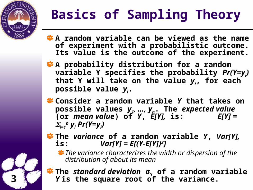
A random variable can be viewed as the name of experiment with a probabilistic outcome. Its value is the outcome of the experiment.

A probability distribution for a random variable Y specifies the probability Pr(Y=yi) that Y will take on the value yi, for each possible value yi.

Consider a random variable Y that takes on possible values y1, …, yn. The expected value (or mean value) of Y, E[Y], is:

E[Y] = i=1n yi Pr(Y=yi)

The variance of a random variable Y, Var[Y], is: Var[Y] = E[(Y-E[Y])2]

The variance characterizes the width or dispersion of the distribution of about its mean

The standard deviation σY of a random variable Y is the square root of the variance.

4

Basics of Sampling Theory: Binomial distribution

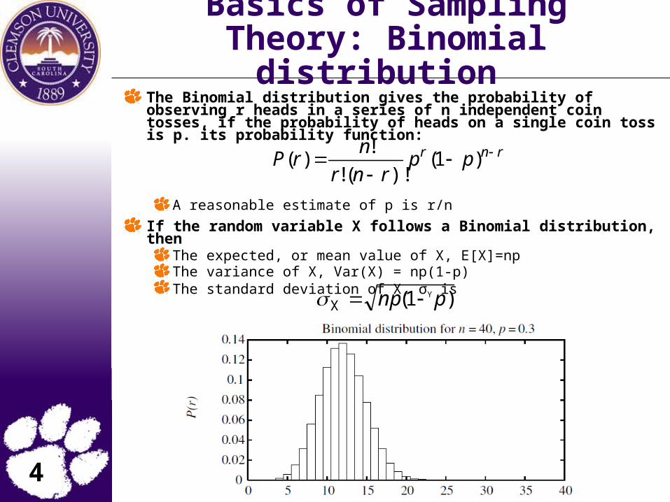
The Binomial distribution gives the probability of observing r heads in a series of n independent coin tosses, if the probability of heads on a single coin toss is p. its probability function:

A reasonable estimate of p is r/n

If the random variable X follows a Binomial distribution, thenThe expected, or mean value of X, E[X]=npThe variance of X, Var(X) = np(1-p)The standard deviation of X, σY is

rnr pprnr

nrP

)1(

)!(!

!)(

)1(X pnp

5

Basics of Sampling Theory: Normal distribution

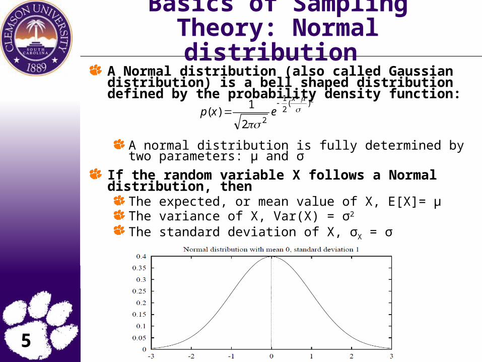
A Normal distribution (also called Gaussian distribution) is a bell shaped distribution defined by the probability density function:

A normal distribution is fully determined by two parameters: μ and σ

If the random variable X follows a Normal distribution, then

The expected, or mean value of X, E[X]= μThe variance of X, Var(X) = σ2

The standard deviation of X, σX = σ

2)(2

1

22

1)(

x

exp

6

Confidence Interval

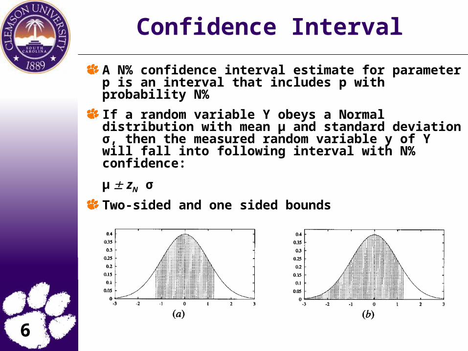
A N% confidence interval estimate for parameter p is an interval that includes p with probability N%

If a random variable Y obeys a Normal distribution with mean μ and standard deviation σ, then the measured random variable y of Y will fall into following interval with N% confidence:

μ zN σ

Two-sided and one sided bounds

7

Basics of Sampling Theory: Central Limit Theorem

The Central Limit Theorem is a theorem stating that the sum of a large number of independent, identically distributed random variable approximately follows a Normal distribution.

Consider a set of independent, identically distributed random variable Yi,…Yn. All governed by an arbitrary probability distribution with mean u and standard deviation σ. Define the sample mean

Central Limit Theorem: As n->∞, the distribution governing Y approaches a Normal distribution, with mean u and variance σ2 /n

n

iiYn

Y1

1

8

Evaluating Hypotheses: Motivation

Evaluating the performance of learning systems is important because:

Learning systems are usually designed to predict the class of “future” unlabeled data points.In some cases, evaluating hypotheses is an integral part of the learning process (example, when pruning a decision tree)

9

Difficulties in Evaluating Hypotheses when only limited data are available

Bias in the estimate: The observed accuracy of the learned hypothesis over the training examples is a poor estimator of its accuracy over future examples

we test the hypothesis on a test set chosen independently of the training set and the hypothesis.

Variance in the estimate: Even with a separate test set, the measured accuracy can vary from the true accuracy, depending on the makeup of the particular set of test examples. The smaller the test set, the greater the expected variance.

10

Questions Considered

Given the observed accuracy of a hypothesis over a limited sample of data, how well does this estimate its accuracy over additional examples?

Given that one hypothesis outperforms another over some sample data, how probable is it that this hypothesis is more accurate, in general?

When data is limited what is the best way to use this data to both learn a hypothesis and estimate its accuracy?

11

Two Definition of Error

Definition 1: The sample error (denoted errors(h)) of hypothesis h with respect to target function f and data sample S is:

errors(h)= 1/n xS(f(x),h(x))

where n is the number of examples in S, and the quantity (f(x),h(x)) is 1 if f(x) h(x), and 0, otherwise.

Definition 2: The true error (denoted errorD(h)) of hypothesis h with respect to target function f and distribution D, is the probability that h will misclassify an instance drawn at random according to D.

errorD(h)= PrxD[f(x) h(x)]

12

Problems Estimating Error

Bias: if S is the training set, errors(h) is optimistically biased

Bias = E[errors(h)]-errorD(h)

For unbiased estimate, h and S must be chose independently

Variance: even with unbiased S, errors(h) may still vary from errorD(h)

13

Estimating Hypothesis Accuracy

Two Questions of Interest:

Given a hypothesis h and a data sample containing n examples drawn at random according to distribution D, what is the best estimate of the accuracy of h over future instances drawn from the same distribution? ==> sample vs. true errorWhat is the probable error in this accuracy estimate? ==> confidence intervals

14

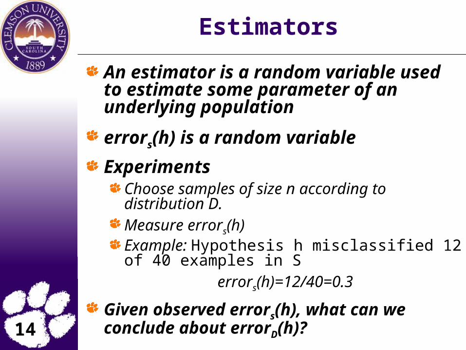
Estimators

An estimator is a random variable used to estimate some parameter of an underlying population

errors(h) is a random variable

ExperimentsChoose samples of size n according to distribution D.Measure errors(h)Example: Hypothesis h misclassified 12 of 40 examples in S

errors(h)=12/40=0.3

Given observed errors(h), what can we conclude about errorD(h)?

15

Estimators, Bias and Variance

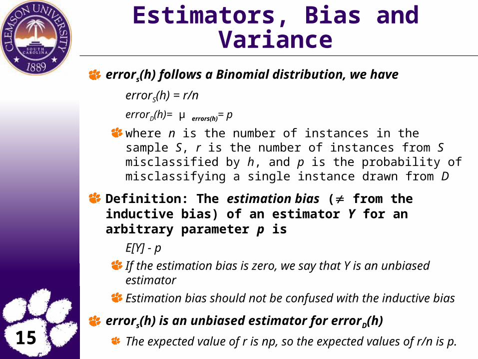
errors(h) follows a Binomial distribution, we have

errorS(h) = r/n

errorD(h)= μ errors(h)= p

where n is the number of instances in the sample S, r is the number of instances from S misclassified by h, and p is the probability of misclassifying a single instance drawn from D

Definition: The estimation bias ( from the inductive bias) of an estimator Y for an arbitrary parameter p is

E[Y] - p

If the estimation bias is zero, we say that Y is an unbiased estimator

Estimation bias should not be confused with the inductive bias

errors(h) is an unbiased estimator for errorD(h)

The expected value of r is np, so the expected values of r/n is p.

16

Estimators, Bias and Variance

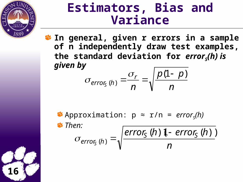
In general, given r errors in a sample of n independently draw test examples, the standard deviation for errorS(h) is given by

Approximation: p ≈ r/n = errorS(h)

Then:

n

pp

nr

herrorS

)1()(

n

herrorherror SSherrorS

))(1)(()(

17

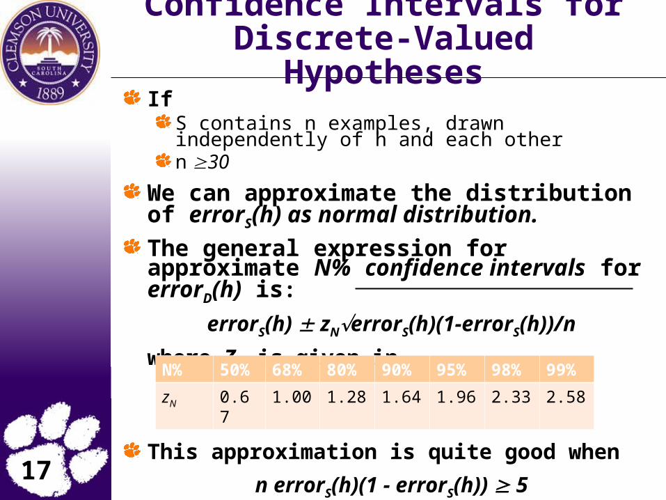
Confidence Intervals for Discrete-Valued Hypotheses

IfS contains n examples, drawn independently of h and each othern 30

We can approximate the distribution of errorS(h) as normal distribution.

The general expression for approximate N% confidence intervals for errorD(h) is:

errorS(h) zNerrorS(h)(1-errorS(h))/n

where ZN is given in

This approximation is quite good when

n errorS(h)(1 - errorS(h)) 5

N% 50% 68% 80% 90% 95% 98% 99%

zN 0.67 1.00 1.28 1.64 1.96 2.33 2.58

18

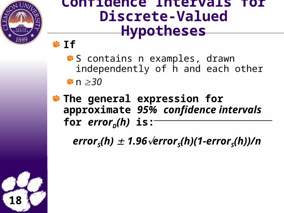
Confidence Intervals for Discrete-Valued Hypotheses

IfS contains n examples, drawn independently of h and each othern 30

The general expression for approximate 95% confidence intervals for errorD(h) is:

errorS(h) 1.96errorS(h)(1-errorS(h))/n

19

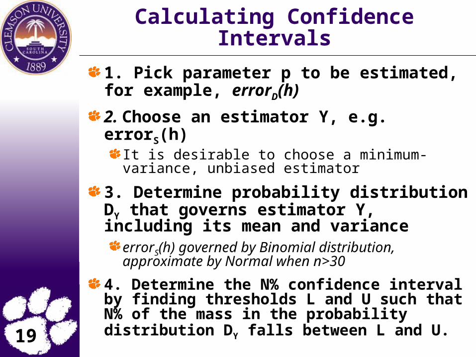
Calculating Confidence Intervals

1. Pick parameter p to be estimated, for example, errorD(h)

2. Choose an estimator Y, e.g. errorS(h)It is desirable to choose a minimum-variance, unbiased estimator

3. Determine probability distribution DY that governs estimator Y, including its mean and variance

errorS(h) governed by Binomial distribution, approximate by Normal when n>30

4. Determine the N% confidence interval by finding thresholds L and U such that N% of the mass in the probability distribution DY falls between L and U.

20

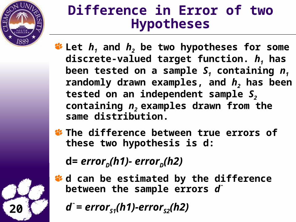
Difference in Error of two Hypotheses

Let h1 and h2 be two hypotheses for some discrete-valued target function. h1 has been tested on a sample S1 containing n1 randomly drawn examples, and h2 has been tested on an independent sample S2 containing n2 examples drawn from the same distribution.

The difference between true errors of these two hypothesis is d:

d= errorD(h1)- errorD(h2)

d can be estimated by the difference between the sample errors dˆ

dˆ = errorS1(h1)-errorS2(h2)

21

Difference in Error of two Hypotheses

The difference of two Normal distribution is also a Normal distribution, then dˆ will also can be approximated by a normal distribution and the variance of this distribution is the sum of the variance of errorS1(h1) and errorS2(h2):

The approximate N% confidence interval for d is:

2

))2(1)(2(

1

))1(1)(1( 22112ˆ

n

herrorherror

n

herrorherror SSSSd

2

))2(1)(2(

1

))1(1)(1(ˆ 2211

n

herrorherror

n

herrorherrorzd SSSSN

22

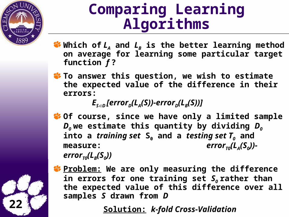
Comparing Learning Algorithms

Which of LA and LB is the better learning method on average for learning some particular target function f ?

To answer this question, we wish to estimate the expected value of the difference in their errors: ESD [errorD(LA(S))-errorD(LB(S))]

Of course, since we have only a limited sample D0 we estimate this quantity by dividing D0 into a training set S0 and a testing set T0 and measure: errorT0(LA(S0))-errorT0(LB(S0))

Problem: We are only measuring the difference in errors for one training set S0 rather than the expected value of this difference over all samples S drawn from D

Solution: k-fold Cross-Validation

23

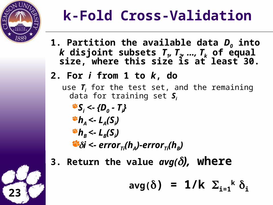
k-Fold Cross-Validation

1. Partition the available data D0 into k disjoint subsets T1, T2, …, Tk of equal size, where this size is at least 30.

2. For i from 1 to k, douse Ti for the test set, and the remaining data for

training set Si

Si <- {D0 - Ti}hA <- LA(Si)hB <- LB(Si)i <- errorTi(hA)-errorTi(hB)

3. Return the value avg(), where avg() = 1/k i=1

k i

24

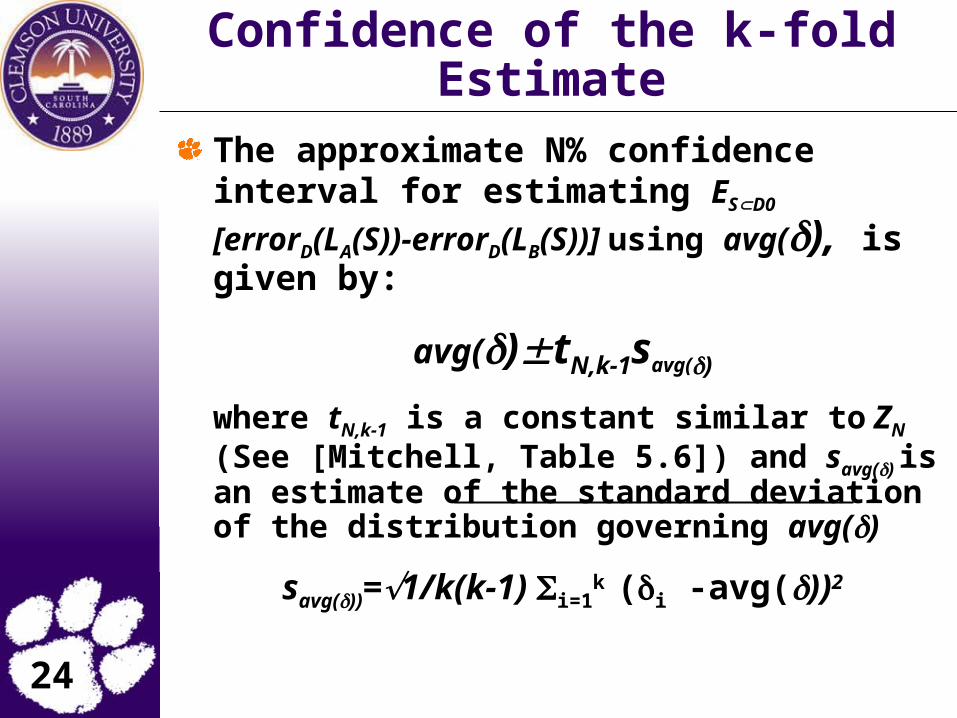
Confidence of the k-fold Estimate

The approximate N% confidence interval for estimating ESD0 [errorD(LA(S))-errorD(LB(S))]

using avg(), is given by:

avg()tN,k-1savg()

where tN,k-1 is a constant similar to ZN (See [Mitchell, Table 5.6]) and savg() is an estimate of the standard deviation of the distribution governing avg()

savg())=1/k(k-1) i=1k (i -avg())2