CPSC 340:Machine Learning and Data Mining

Multi-Class Regression

Fall 2016

Admin

• Midterm:

– Grades/solutions will be posted later this week.

• Assignment 4:

– Posted, due November 14.

• Extra office hours:

– Thursdays from 4:30-5:30 in ICICS X836.

Last Time: L1-Regularization

• We discussed L1-regularization:

– Also known as “LASSO” and “basis pursuit denoising”.

– Regularizes ‘w’ so we decrease our test error (like L2-regularization).

– Yields sparse ‘w’ so it selects features (like L0-regularization).

• Properties:

– It’s convex and fast to minimize (proximal-gradient).

– Solution is not unique.

– Tends to yield false positives.

Extensions of L1-Regularization

• “Elastic net” uses L2-regularization plus L1-regularization.– Solution is still sparse but is now unique.

– Slightly better with feature dependence: selects both “mom” and “mom2”.

• “Bolasso” runs L1-regularization on bootstrap samples.– Selects features that are non-zero in all samples.

– Much less sensitive to false positives.

• There are many non-convex regularizers (square-root, “SCAD”):– Much less sensitive to false positives.

– But computing global minimum is hard.

Last: Maximum Likelihood Estimation

• We discussed computing ‘w’ by maximum likelihood estimation (MLE):

• This is equivalent to minimizing negative log-likelihood (NLL):

• For logistic regression, probability is wTxi passed through sigmoid.

• And MLE is minimum of:

• With regularization, similar to SVMs. But gives probabilities.

Maximum Likelihood and Least Squares

• Many of our objective functions can be written as an MLE.

• For example, consider Gaussian likelihood with mean of wTxi:

• So the NLL is given by:

Maximum Likelihood and Least Squares

• Many of our objective functions can be written as an MLE.

• For example, consider Gaussian likelihood we mean of wTxi:

• So we can minimize NLL by minimizing:

• So least squares is MLE under Gaussian likelihood.– With a Laplace likelihood you would absolute error.

Problem with Maximum Likelihood Estimation

• Maximum likelihood estimate maximizes:

• It’s is a bit weird:– “Find the ‘w’ that makes ‘y’ have the highest probability given ‘X’ and ‘w’.”

• A problem with MLE: – ‘y’ could be very likely for some very unlikely ‘w’.

– E.g., complex model that overfit by memorizing the data.

• What we really want:– “Find the ‘w’ that has the highest probability given ‘X’ and ‘y’.”

Maximum a Posteriori (MAP) Estimation

• Maximum a posteriori (MAP) maximizes what we want:

• Using Bayes’ rule, we have

Maximum a Posteriori (MAP) Estimation

• Maximum a posteriori (MAP) maximizes what we want:

• Prior p(h) is ‘belief’ that ‘w’ is the correct before seeing data:

– Can take into account that complex models can overfit.

• If we again minimize the negative of the logarithm, we get:

MAP Estimation and Regularization

• While many losses are equivalent to NLLs, many regularizers are equivalent to negative log-priors.

• Assume each wj comes from a Gaussian (0-mean, 1/λ variance):

• Then the log-prior is:

• And negative log-prior over all ‘j’ is:

MAP Estimation and Regularization

• MAP estimation gives link between probabilities and loss functions.

– Gaussian likelihood and Gaussian prior gives L2-regularized least squares.

– Sigmoid likelihood and Gaussian prior gives L2-regularizedlogistic regression:

Why do we care about MLE and MAP?

• Unified way of thinking about many of our tricks?– Laplace smoothing in naïve Bayes can be viewed as regularization.

• Remember our two ways to reduce complexity of a model:– Model averaging (ensemble methods).

– Regularization (linear models).

• “Fully”-Bayesian methods combine both of these.– Average over all models, weighted by posterior (which includes regularizer).

– Very powerful class of models we’ll cover in CPSC 540.

• Sometimes it’s easier to define a likelihood than a loss function.– We’ll do this for multi-class classification.

Multi-Label Classification

• We’ve been considering supervised learning with a single label:

• E.g., is there a cat in this image or not?

https://www.youtube.com/watch?v=tntOCGkgt98

Multi-Label Classification

• In multi-label classification we want to predict ‘k’ binary labels:

• E.g., which of the ‘k’ objects are in this image?

http://image-net.org/challenges/LSVRC/2013/

Multi-Label Classification

• Approach 1:

– Treat {1,-1,1,1,-1} as the binary label 10110.

– Problem is that with ‘k’ labels you have 2k classes.

• Only useful if ‘k’ is very small.

Multi-Label Classification

• Approach 2:

– Fit a binary classifier for each column ‘c’ of Y, using column as labels.

• If we use a linear model, each classifier has a weights wc.

• Let’s put the wc together into a matrix ‘W’:

Multi-Label Classification

• Fancier methods model correlations between yi or between the wc.

Multi-Class Classification

• Multi-class classification: special case where each yi has 1 non-zero.

Multi-Class Classification and “One vs. All”

• Multi-class classification: special case where each yi has 1 non-zero.

– Now we can code yi as a discrete number {1,2,3,…} giving class ‘k’.

• One vs. all multi-class approach uses naïve multi-label approach:

– Independently fit parameters ‘wc’ of a linear model for each class ‘c’.

• Each ‘wc’ tries to predict +1 for class ‘c’ and -1 for all others.

Multi-Class Classification and “One vs. All”

• But prediction WTxi might have multiple +1 values.

• To predict the “best” label, choose ‘c’ with largest value of wcTxi.

Multi-Class Classification and “One vs. All”

• But we only trained wc to get the correct sign of yic:

– We didn’t train the wc so that the largest wcTxi would be yi.

Multinomial Logistic Regression

• Can we define a loss function so that largest wcTxi gives yi?

• In the multi-label logistic regression model we used:

• The multinomial logistic regression model uses the same idea:

• But now need to sum over ‘k’ classes to get a valid probability:

Multinomial Logistic Regression

• So multinomial logistic regression uses:

• Which is also known as the softmax function.

• Now that we have a probability, the MLE gives a loss function:

Losses for Other Discrete Labels

• MLE/MAP gives loss for classification with basic discrete labels:– Logistic regression for binary labels {“spam”, “not spam”}.

– Softmax regression for multi-class {“spam”, “not spam”, “important”}.

• But MLE/MAP lead to losses with other discrete labels:– Ordinal: {1 star, 2 stars, 3 stars, 4 stars, 5 stars}.

– Counts: 602 ‘likes’.

• We can also use ratios of probabilities to define more losses:– Multi-class SVMs (similar to softmax, but generalizes hinge loss).

– Ranking: Difficulty(A3) > Difficulty(A4) > Difficulty (A2) > DifficultyA(1).

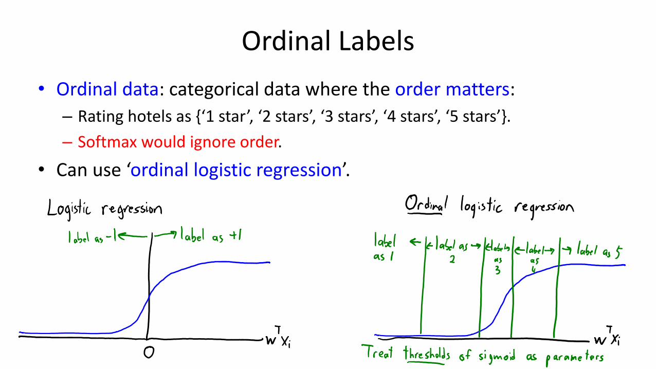
Ordinal Labels

• Ordinal data: categorical data where the order matters:

– Rating hotels as {‘1 star’, ‘2 stars’, ‘3 stars’, ‘4 stars’, ‘5 stars’}.

– Softmax would ignore order.

• Can use ‘ordinal logistic regression’.

Count Labels

• Count data: predict the number of times something happens.

– For example, yi = “602” Facebok likes.

• Softmax/ordinal require finite number of possible labels.

• We probably don’t want separate parameter for ‘654’ and ‘655’.

• Poisson regression: use probability from Poisson count distribution.

– Many variations exist.

Summary

• -log(probability) lets us to define loss from any probability.

– Special cases are least squares, least absolute error, and logistic regression.

• MAP estimation directly models p(w | X, y).

– Gives probabilistic interpretation to regularization.

• Softmax loss is natural generalization of logistic regression.

• Discrete losses for weird scenarios are possible using MLE/MAP:

– Ordinal logistic regression, Poisson regression.

• Next time:

– What ‘parts’ are your personality made of?

Bonus Slide: Multi-Class SVMs

Bonus Slide: Ranking