coxeter groups and hopf algebras i marcelo aguiar and swapneel
TRANSCRIPT

Coxeter groups and Hopf algebras I
Marcelo Aguiar and Swapneel Mahajan
Department of Mathematics, Texas A&M University, College Station,
Texas 77843, USA
E-mail address : [email protected]: http://www.math.tamu.edu/∼maguiar
Department of Mathematics, Indian Institute of Technology, Powai,
Mumbai 400 076, India
E-mail address : [email protected]: http://www.math.iitb.ac.in/∼swapneel

2000 Mathematics Subject Classification. 05E05, 06A11, 06A15, 16W30, 51E24.
Key words and phrases. Coxeter group; descent; global descent; hyperplanearrangement; left regular band (LRB); projection map; projection poset; lunes; shuffles;bilinear forms; descent algebra; semisimple; Hopf algebra; (quasi) symmetric functions;
(co)algebra axioms; (nested) set partitions; (nested) set compositions; (co)free(co)algebra.

Foreword
In the study of a mathematical system, algebraic structures allow for the discovery ofmore information. This is the motor behind the success of many areas of mathematicssuch as algebraic geometry, algebraic combinatorics, algebraic topology and others. Thiswas certainly the motivation behind the observation of G.-C. Rota stating that variouscombinatorial objects possess natural product and coproduct structures. These struc-tures give rise to a graded Hopf algebra, which is usually referred to as a combinatorialHopf algebra. Typically, it is a graded vector space where the homogeneous componentsare spanned by finite sets of combinatorial objects of a given type and the algebraicstructures are given by some constructions on those objects.
Recent foundational work has constructed many interesting combinatorial Hopf al-gebras and uncovered new connections between diverse subjects such as combinatorics,algebra, geometry, and theoretical physics. This has expanded the new and vibrantsubject of combinatorial Hopf algebras. To give a few instances:
• Connes and Kreimer showed that a certain renormalization problem in quantumfield theory can be encoded and solved using a Hopf algebra indexed by rootedtrees.
• Loday and Ronco showed that a Hopf algebra indexed by planar binary trees is thefree dendriform algebra on one generator. This is true for many types of algebras;the free algebra on one generator is a combinatorial Hopf algebra.
• In the context of polytope theory, some interesting enumerative combinatorial in-variants induce a Hopf morphism from a Hopf algebra of posets to the Hopf algebraof quasi-symmetric functions.
• Krob and Thibon showed that the representation theory of the Hecke algebrasat q = 0 is intimately related to the Hopf algebra structure of quasi-symmetricfunctions and non-commutative symmetric functions.
Some of the latest research in these areas has been the subject of a series of recentmeetings, including an AMS/CMS meeting in Montre al in May 2002, a BIRS workshopin Banff in August 2004, and a CIRM workshop in Luminy in April 2005. It was suggestedat the BIRS meeting that the draft text of M. Aguiar and S. Mahajan be expanded intothe first monograph on the subject. Both are outstanding communicators. Their unifiedgeometric approach using Coxeter complexes and projection maps allows us to constructmany of the combinatorial Hopf algebras currently under study and further to understandtheir properties (freeness, cofreeness, etc.) and to describe morphisms among them.
The current monograph is the result of this great effort and it is for me a greatpleasure to introduce it.
Nantel BergeronCanada Research ChairYork University
3

4

Contents
Preface i
0.1 The first part: Chapters 1-3 . . . . . . . . . . . . . . . . . . . . . . . . . . i0.2 The second part: Chapters 4-8 . . . . . . . . . . . . . . . . . . . . . . . . i0.3 Future work . . . . . . . . . . . . . . . . . . . . . . . . . . . . . . . . . . . i0.4 Acknowledgements . . . . . . . . . . . . . . . . . . . . . . . . . . . . . . . ii0.5 Notation . . . . . . . . . . . . . . . . . . . . . . . . . . . . . . . . . . . . . ii
1 Coxeter groups 1
1.1 Regular cell complexes and simplicial complexes . . . . . . . . . . . . . . 11.1.1 Gate property . . . . . . . . . . . . . . . . . . . . . . . . . . . . . . 11.1.2 Link and join . . . . . . . . . . . . . . . . . . . . . . . . . . . . . . 2
1.2 Hyperplane arrangements . . . . . . . . . . . . . . . . . . . . . . . . . . . 21.2.1 Faces . . . . . . . . . . . . . . . . . . . . . . . . . . . . . . . . . . 21.2.2 Flats . . . . . . . . . . . . . . . . . . . . . . . . . . . . . . . . . . . 31.2.3 Spherical picture . . . . . . . . . . . . . . . . . . . . . . . . . . . . 31.2.4 Gate property and other facts . . . . . . . . . . . . . . . . . . . . . 4
1.3 Reflection arrangements . . . . . . . . . . . . . . . . . . . . . . . . . . . . 41.3.1 Finite reflection groups . . . . . . . . . . . . . . . . . . . . . . . . 41.3.2 Types of faces . . . . . . . . . . . . . . . . . . . . . . . . . . . . . . 51.3.3 The Coxeter diagram . . . . . . . . . . . . . . . . . . . . . . . . . 51.3.4 The distance map . . . . . . . . . . . . . . . . . . . . . . . . . . . 61.3.5 The Bruhat order . . . . . . . . . . . . . . . . . . . . . . . . . . . . 61.3.6 The descent algebra: A geometric approach . . . . . . . . . . . . . 71.3.7 Link and join . . . . . . . . . . . . . . . . . . . . . . . . . . . . . . 7
1.4 The Coxeter group of type An−1 . . . . . . . . . . . . . . . . . . . . . . . 81.4.1 The braid arrangement . . . . . . . . . . . . . . . . . . . . . . . . 81.4.2 Types of faces . . . . . . . . . . . . . . . . . . . . . . . . . . . . . . 91.4.3 Set compositions and partitions . . . . . . . . . . . . . . . . . . . . 91.4.4 The Bruhat order . . . . . . . . . . . . . . . . . . . . . . . . . . . . 10
2 Left regular bands 11
2.1 Why LRBs? . . . . . . . . . . . . . . . . . . . . . . . . . . . . . . . . . . . 112.2 Faces and flats . . . . . . . . . . . . . . . . . . . . . . . . . . . . . . . . . 12
2.2.1 Faces . . . . . . . . . . . . . . . . . . . . . . . . . . . . . . . . . . 122.2.2 Flats . . . . . . . . . . . . . . . . . . . . . . . . . . . . . . . . . . . 122.2.3 Chambers . . . . . . . . . . . . . . . . . . . . . . . . . . . . . . . . 122.2.4 Examples . . . . . . . . . . . . . . . . . . . . . . . . . . . . . . . . 13
2.3 Pointed faces and lunes . . . . . . . . . . . . . . . . . . . . . . . . . . . . 132.3.1 Pointed faces . . . . . . . . . . . . . . . . . . . . . . . . . . . . . . 132.3.2 Lunes . . . . . . . . . . . . . . . . . . . . . . . . . . . . . . . . . . 132.3.3 The relation of Q and Z with Σ and L . . . . . . . . . . . . . . . . 142.3.4 Lunar regions . . . . . . . . . . . . . . . . . . . . . . . . . . . . . . 14
5

6 CONTENTS
2.3.5 Examples . . . . . . . . . . . . . . . . . . . . . . . . . . . . . . . . 152.4 Link and join of LRBs . . . . . . . . . . . . . . . . . . . . . . . . . . . . . 16
2.4.1 SubLRB and quotient LRB . . . . . . . . . . . . . . . . . . . . . . 172.4.2 Product of LRBs . . . . . . . . . . . . . . . . . . . . . . . . . . . . 17
2.5 Bilinear forms related to a LRB . . . . . . . . . . . . . . . . . . . . . . . . 172.5.1 The bilinear form on KQ . . . . . . . . . . . . . . . . . . . . . . . 172.5.2 The pairing between KQ and KΣ . . . . . . . . . . . . . . . . . . . 182.5.3 The bilinear form on KΣ . . . . . . . . . . . . . . . . . . . . . . . 192.5.4 The bilinear form on KL . . . . . . . . . . . . . . . . . . . . . . . . 192.5.5 The nondegeneracy of the form on KL . . . . . . . . . . . . . . . . 20
2.6 Bilinear forms related to a Coxeter group . . . . . . . . . . . . . . . . . . 212.6.1 The bilinear form on (KΣ)W . . . . . . . . . . . . . . . . . . . . . 222.6.2 The bilinear form on (KL)W and its nondegeneracy . . . . . . . . 23
2.7 Projection posets . . . . . . . . . . . . . . . . . . . . . . . . . . . . . . . . 242.7.1 Definition and examples . . . . . . . . . . . . . . . . . . . . . . . . 242.7.2 Elementary facts . . . . . . . . . . . . . . . . . . . . . . . . . . . . 25
3 Hopf algebras 27
3.1 Hopf algebras . . . . . . . . . . . . . . . . . . . . . . . . . . . . . . . . . . 273.1.1 Cofree graded coalgebras . . . . . . . . . . . . . . . . . . . . . . . 273.1.2 The coradical filtration . . . . . . . . . . . . . . . . . . . . . . . . 283.1.3 Antipode . . . . . . . . . . . . . . . . . . . . . . . . . . . . . . . . 28
3.2 Hopf algebras: Examples . . . . . . . . . . . . . . . . . . . . . . . . . . . . 293.2.1 The Hopf algebra Λ . . . . . . . . . . . . . . . . . . . . . . . . . . 293.2.2 The Hopf algebra QΛ . . . . . . . . . . . . . . . . . . . . . . . . . 313.2.3 The Hopf algebra NΛ . . . . . . . . . . . . . . . . . . . . . . . . . 323.2.4 The duality between QΛ and NΛ . . . . . . . . . . . . . . . . . . . 32
4 A brief overview 33
4.1 Abstract: Chapter 5 . . . . . . . . . . . . . . . . . . . . . . . . . . . . . . 334.2 Abstract: Chapter 6 . . . . . . . . . . . . . . . . . . . . . . . . . . . . . . 344.3 Abstract: Chapters 7 and 8 . . . . . . . . . . . . . . . . . . . . . . . . . . 35
5 The descent theory for Coxeter groups 37
5.1 Introduction . . . . . . . . . . . . . . . . . . . . . . . . . . . . . . . . . . . 375.1.1 The first part: Sections 5.2-5.5 . . . . . . . . . . . . . . . . . . . . 375.1.2 The second part: Sections 5.6-5.7 . . . . . . . . . . . . . . . . . . . 38
5.2 The descent theory for Coxeter groups . . . . . . . . . . . . . . . . . . . . 395.2.1 Preliminaries . . . . . . . . . . . . . . . . . . . . . . . . . . . . . . 395.2.2 Summary . . . . . . . . . . . . . . . . . . . . . . . . . . . . . . . . 395.2.3 The posets Z and L . . . . . . . . . . . . . . . . . . . . . . . . . . 405.2.4 The partial orders on C × C and Q . . . . . . . . . . . . . . . . . . 405.2.5 The map Road . . . . . . . . . . . . . . . . . . . . . . . . . . . . . 425.2.6 The map GRoad . . . . . . . . . . . . . . . . . . . . . . . . . . . . 435.2.7 The map Θ . . . . . . . . . . . . . . . . . . . . . . . . . . . . . . . 445.2.8 Connection among the three maps . . . . . . . . . . . . . . . . . . 45
5.3 The coinvariant descent theory for Coxeter groups . . . . . . . . . . . . . 465.3.1 The map des . . . . . . . . . . . . . . . . . . . . . . . . . . . . . . 465.3.2 The map gdes . . . . . . . . . . . . . . . . . . . . . . . . . . . . . . 475.3.3 The map θ . . . . . . . . . . . . . . . . . . . . . . . . . . . . . . . 475.3.4 Connection among the three maps . . . . . . . . . . . . . . . . . . 485.3.5 Shuffles . . . . . . . . . . . . . . . . . . . . . . . . . . . . . . . . . 495.3.6 Sets related to the product in the M basis of SΛ . . . . . . . . . . 51
5.4 The example of type An−1 . . . . . . . . . . . . . . . . . . . . . . . . . . . 52

CONTENTS 7
5.4.1 The posets Σn and Ln . . . . . . . . . . . . . . . . . . . . . . . . . 535.4.2 The posets Qn and Zn . . . . . . . . . . . . . . . . . . . . . . . . . 535.4.3 The quotient posets Q
nand L
n. . . . . . . . . . . . . . . . . . . . 54
5.4.4 The maps Road, GRoad and Θ . . . . . . . . . . . . . . . . . . . . 545.4.5 The maps des, gdes and θ . . . . . . . . . . . . . . . . . . . . . . . 555.4.6 Shuffles . . . . . . . . . . . . . . . . . . . . . . . . . . . . . . . . . 56
5.5 The toy example of type A×(n−1)1 . . . . . . . . . . . . . . . . . . . . . . . 56
5.5.1 The posets Σn and Ln . . . . . . . . . . . . . . . . . . . . . . . . . 565.5.2 The posets Qn and Zn . . . . . . . . . . . . . . . . . . . . . . . . . 575.5.3 The quotient posets Q
nand L
n. . . . . . . . . . . . . . . . . . . . 57
5.5.4 The maps Des, GDes and Θ . . . . . . . . . . . . . . . . . . . . . . 585.5.5 The maps des, gdes and θ . . . . . . . . . . . . . . . . . . . . . . . 58
5.6 The commutative diagram (5.8) . . . . . . . . . . . . . . . . . . . . . . . . 585.6.1 The objects in diagram (5.8) . . . . . . . . . . . . . . . . . . . . . 595.6.2 The maps s, Θ and Road . . . . . . . . . . . . . . . . . . . . . . . 605.6.3 The bilinear form on KQ . . . . . . . . . . . . . . . . . . . . . . . 615.6.4 The top half of diagram (5.8) . . . . . . . . . . . . . . . . . . . . . 625.6.5 The maps supp, lune and base∗ . . . . . . . . . . . . . . . . . . . . 625.6.6 The dual maps supp∗, lune∗ and base . . . . . . . . . . . . . . . . 635.6.7 The maps Φ and Υ . . . . . . . . . . . . . . . . . . . . . . . . . . . 635.6.8 The bottom half of diagram (5.8) . . . . . . . . . . . . . . . . . . . 635.6.9 The algebra KL . . . . . . . . . . . . . . . . . . . . . . . . . . . . . 64
5.7 The coinvariant commutative diagram (5.17) . . . . . . . . . . . . . . . . 655.7.1 The objects in diagram (5.17) . . . . . . . . . . . . . . . . . . . . . 665.7.2 The maps from invariants . . . . . . . . . . . . . . . . . . . . . . . 675.7.3 The maps to coinvariants . . . . . . . . . . . . . . . . . . . . . . . 695.7.4 The maps in diagram (5.17) . . . . . . . . . . . . . . . . . . . . . . 705.7.5 The algebra KL . . . . . . . . . . . . . . . . . . . . . . . . . . . . . 715.7.6 A different viewpoint relating diagrams (5.8) and (5.17) . . . . . . 72
6 The construction of Hopf algebras 75
6.1 Introduction . . . . . . . . . . . . . . . . . . . . . . . . . . . . . . . . . . . 756.1.1 A diagram of vector spaces for a LRB . . . . . . . . . . . . . . . . 756.1.2 A diagram of coalgebras and algebras for a family of LRBs . . . . 766.1.3 The example of type A . . . . . . . . . . . . . . . . . . . . . . . . 77
6.2 The Hopf algebras of type A . . . . . . . . . . . . . . . . . . . . . . . . . 796.2.1 Summary . . . . . . . . . . . . . . . . . . . . . . . . . . . . . . . . 796.2.2 The structure of the Hopf algebras of type A . . . . . . . . . . . . 806.2.3 Set compositions . . . . . . . . . . . . . . . . . . . . . . . . . . . . 806.2.4 The Hopf algebra PΠ . . . . . . . . . . . . . . . . . . . . . . . . . 826.2.5 The Hopf algebra MΠ . . . . . . . . . . . . . . . . . . . . . . . . . 826.2.6 Nested set compositions . . . . . . . . . . . . . . . . . . . . . . . . 836.2.7 The Hopf algebra QΠ . . . . . . . . . . . . . . . . . . . . . . . . . 846.2.8 The Hopf algebra NΠ . . . . . . . . . . . . . . . . . . . . . . . . . 846.2.9 Set partitions . . . . . . . . . . . . . . . . . . . . . . . . . . . . . . 856.2.10 The Hopf algebra ΠL∗ . . . . . . . . . . . . . . . . . . . . . . . . . 856.2.11 The Hopf algebra ΠL . . . . . . . . . . . . . . . . . . . . . . . . . . 866.2.12 Nested set partitions . . . . . . . . . . . . . . . . . . . . . . . . . . 866.2.13 The Hopf algebra ΠZ∗ . . . . . . . . . . . . . . . . . . . . . . . . . 876.2.14 The Hopf algebra ΠZ . . . . . . . . . . . . . . . . . . . . . . . . . . 876.2.15 The Hopf algebra SΠ . . . . . . . . . . . . . . . . . . . . . . . . . . 876.2.16 The Hopf algebra RΠ . . . . . . . . . . . . . . . . . . . . . . . . . 88
6.3 The coalgebra axioms and examples . . . . . . . . . . . . . . . . . . . . . 886.3.1 The coalgebra axioms . . . . . . . . . . . . . . . . . . . . . . . . . 89

8 CONTENTS
6.3.2 The warm-up example of compositions . . . . . . . . . . . . . . . . 906.3.3 The motivating example of type An−1 . . . . . . . . . . . . . . . . 91
6.3.4 The example of type A×(n−1)1 . . . . . . . . . . . . . . . . . . . . . 95
6.4 From coalgebra axioms to coalgebras . . . . . . . . . . . . . . . . . . . . . 966.4.1 The coproducts . . . . . . . . . . . . . . . . . . . . . . . . . . . . . 966.4.2 Coassociativity of the coproducts . . . . . . . . . . . . . . . . . . . 966.4.3 Useful results for coassociativity . . . . . . . . . . . . . . . . . . . 97
6.5 Construction of coalgebras . . . . . . . . . . . . . . . . . . . . . . . . . . . 986.5.1 Examples . . . . . . . . . . . . . . . . . . . . . . . . . . . . . . . . 996.5.2 The coproducts and local and global vertices . . . . . . . . . . . . 996.5.3 The coalgebra P . . . . . . . . . . . . . . . . . . . . . . . . . . . . 1006.5.4 The coalgebraM . . . . . . . . . . . . . . . . . . . . . . . . . . . . 1026.5.5 The coalgebra Q . . . . . . . . . . . . . . . . . . . . . . . . . . . . 1036.5.6 The coalgebra N . . . . . . . . . . . . . . . . . . . . . . . . . . . . 1056.5.7 The coalgebra S . . . . . . . . . . . . . . . . . . . . . . . . . . . . 1066.5.8 The coalgebra R . . . . . . . . . . . . . . . . . . . . . . . . . . . . 1086.5.9 The maps Road : S → Q and Θ : N → R . . . . . . . . . . . . . . 1096.5.10 The coalgebras AZ , AL, AZ∗ and AL∗ . . . . . . . . . . . . . . . . 110
6.6 The algebra axioms and examples . . . . . . . . . . . . . . . . . . . . . . . 1126.6.1 The algebra axioms . . . . . . . . . . . . . . . . . . . . . . . . . . 1126.6.2 The warm-up example of compositions . . . . . . . . . . . . . . . . 1136.6.3 The motivating example of type An−1 . . . . . . . . . . . . . . . . 114
6.6.4 The example of type A×(n−1)1 . . . . . . . . . . . . . . . . . . . . . 116
6.7 From algebra axioms to algebras . . . . . . . . . . . . . . . . . . . . . . . 1166.7.1 The products . . . . . . . . . . . . . . . . . . . . . . . . . . . . . . 1166.7.2 Associativity of the products . . . . . . . . . . . . . . . . . . . . . 1176.7.3 Useful results for associativity . . . . . . . . . . . . . . . . . . . . . 117
6.8 Construction of algebras . . . . . . . . . . . . . . . . . . . . . . . . . . . . 1186.8.1 Examples . . . . . . . . . . . . . . . . . . . . . . . . . . . . . . . . 1186.8.2 The algebra P . . . . . . . . . . . . . . . . . . . . . . . . . . . . . 1196.8.3 The algebraM . . . . . . . . . . . . . . . . . . . . . . . . . . . . . 1216.8.4 The algebra Q . . . . . . . . . . . . . . . . . . . . . . . . . . . . . 1216.8.5 The algebra N . . . . . . . . . . . . . . . . . . . . . . . . . . . . . 1236.8.6 The algebra S . . . . . . . . . . . . . . . . . . . . . . . . . . . . . 1236.8.7 The algebra R . . . . . . . . . . . . . . . . . . . . . . . . . . . . . 1256.8.8 The maps Road : S → Q and Θ : N → R . . . . . . . . . . . . . . 1256.8.9 The algebras AZ , AL, AZ∗ and AL∗ . . . . . . . . . . . . . . . . . 126
7 The Hopf algebra of pairs of permutations 129
7.1 Introduction . . . . . . . . . . . . . . . . . . . . . . . . . . . . . . . . . . . 1297.1.1 The basic setup . . . . . . . . . . . . . . . . . . . . . . . . . . . . . 1297.1.2 The main result . . . . . . . . . . . . . . . . . . . . . . . . . . . . 1297.1.3 The Hopf algebras RΠ and RΛ . . . . . . . . . . . . . . . . . . . . 1307.1.4 Three partial orders on Cn × Cn . . . . . . . . . . . . . . . . . . . . 1317.1.5 The different bases of SΠ and SΛ . . . . . . . . . . . . . . . . . . . 1327.1.6 The proof method and the organization of the chapter . . . . . . . 132
7.2 The Hopf algebra SΠ . . . . . . . . . . . . . . . . . . . . . . . . . . . . . . 1337.2.1 Preliminary definitions . . . . . . . . . . . . . . . . . . . . . . . . . 1337.2.2 Combinatorial definition . . . . . . . . . . . . . . . . . . . . . . . . 1347.2.3 The break and join operations . . . . . . . . . . . . . . . . . . . . 1357.2.4 Geometric definition . . . . . . . . . . . . . . . . . . . . . . . . . . 1357.2.5 The Hopf algebra SΛ . . . . . . . . . . . . . . . . . . . . . . . . . . 136
7.3 The Hopf algebra SΠ in the M basis . . . . . . . . . . . . . . . . . . . . . 1377.3.1 A preliminary result . . . . . . . . . . . . . . . . . . . . . . . . . . 137

CONTENTS 9
7.3.2 Coproduct in the M basis . . . . . . . . . . . . . . . . . . . . . . . 1387.3.3 Product in the M basis . . . . . . . . . . . . . . . . . . . . . . . . 1407.3.4 The switch map on the M basis . . . . . . . . . . . . . . . . . . . 141
7.4 The Hopf algebra SΠ in the S basis . . . . . . . . . . . . . . . . . . . . . 1427.4.1 Two preliminary results . . . . . . . . . . . . . . . . . . . . . . . . 1427.4.2 Coproduct in the S basis . . . . . . . . . . . . . . . . . . . . . . . 1437.4.3 Product in the S basis . . . . . . . . . . . . . . . . . . . . . . . . . 145
7.5 The Hopf algebra RΠ in the H basis . . . . . . . . . . . . . . . . . . . . . 1467.5.1 Coproduct in the H basis . . . . . . . . . . . . . . . . . . . . . . . 1467.5.2 Product in the H basis . . . . . . . . . . . . . . . . . . . . . . . . 1477.5.3 The switch map on the H basis . . . . . . . . . . . . . . . . . . . . 148
8 The Hopf algebra of pointed faces 151
8.1 Introduction . . . . . . . . . . . . . . . . . . . . . . . . . . . . . . . . . . . 1518.1.1 The basic setup . . . . . . . . . . . . . . . . . . . . . . . . . . . . . 1518.1.2 Cofreeness . . . . . . . . . . . . . . . . . . . . . . . . . . . . . . . . 1528.1.3 Three partial orders on Qn . . . . . . . . . . . . . . . . . . . . . . 1528.1.4 The different bases of QΠ . . . . . . . . . . . . . . . . . . . . . . . 1538.1.5 The connection between SΠ and QΠ . . . . . . . . . . . . . . . . . 153
8.2 The Hopf algebra QΠ . . . . . . . . . . . . . . . . . . . . . . . . . . . . . 1538.2.1 Geometric definition . . . . . . . . . . . . . . . . . . . . . . . . . . 1538.2.2 Combinatorial definition . . . . . . . . . . . . . . . . . . . . . . . . 155
8.3 The Hopf algebra PΠ . . . . . . . . . . . . . . . . . . . . . . . . . . . . . 1578.4 The Hopf algebra QΛ of quasi-symmetric functions . . . . . . . . . . . . . 158
Bibliography 161
Author Index 167
Notation Index 169
Subject Index 172

10 CONTENTS

List of Tables
3.1 Hopf algebras, their indexing sets and structure. . . . . . . . . . . . . . . 29
5.1 Combinatorial notions for type An−1. . . . . . . . . . . . . . . . . . . . . 535.2 Vector spaces associated to Σ and their bases. . . . . . . . . . . . . . . . . 595.3 Vector spaces associated to W and their bases. . . . . . . . . . . . . . . . 66
6.1 Graded vector spaces for a family of LRBs. . . . . . . . . . . . . . . . . . 766.2 Hopf algebras and their indexing sets. . . . . . . . . . . . . . . . . . . . . 796.3 Unified description of the Hopf algebras. . . . . . . . . . . . . . . . . . . . 796.4 Hopf algebras and their structure. . . . . . . . . . . . . . . . . . . . . . . 806.5 Local and global vertex of a face and pointed face. . . . . . . . . . . . . . 1006.6 Local and global vertex of a flat and lune. . . . . . . . . . . . . . . . . . . 100
7.1 Hopf algebras and their indexing sets and bases. . . . . . . . . . . . . . . 130
11

12 LIST OF TABLES

List of Figures
1.1 The gate property. . . . . . . . . . . . . . . . . . . . . . . . . . . . . . . . 11.2 The projection map at work. . . . . . . . . . . . . . . . . . . . . . . . . . 41.3 The Coxeter diagrams of type An−1 and Bn. . . . . . . . . . . . . . . . . 61.4 A minimum gallery that illustrates the partial order on W . . . . . . . . . 61.5 The braid arrangement when n = 4. . . . . . . . . . . . . . . . . . . . . . 91.6 The weak left Bruhat order on S4. . . . . . . . . . . . . . . . . . . . . . . 10
2.1 Two low dimensional pictures of the lunar regions reg(P,C) = reg(F,D). . 162.2 The pointed faces (P,C) and (F,D) lie in each other’s lunar regions. . . . 18
4.1 The descent theory. . . . . . . . . . . . . . . . . . . . . . . . . . . . . . . . 334.2 The commutative diagrams. . . . . . . . . . . . . . . . . . . . . . . . . . . 344.3 The external commutative diagrams. . . . . . . . . . . . . . . . . . . . . . 34
5.1 A minimum gallery that illustrates the partial order ≤ on C × C. . . . . . 415.2 The chamber D has a descent with respect to the chamber C at v. . . . . 425.3 The chamber D has a global descent with respect to the chamber C at v. 435.4 A chamber C in the lunar region reg(F,D). . . . . . . . . . . . . . . . . . 445.5 A descent at s for an element w ∈ W . . . . . . . . . . . . . . . . . . . . . 475.6 A global descent at s for an element w ∈W . . . . . . . . . . . . . . . . . . 475.7 The image of the θ map in rank 3. . . . . . . . . . . . . . . . . . . . . . . 485.8 T -shuffles correspond to faces of type T . . . . . . . . . . . . . . . . . . . . 505.9 The set S0
w(x). . . . . . . . . . . . . . . . . . . . . . . . . . . . . . . . . . 51
6.1 The break map bF . . . . . . . . . . . . . . . . . . . . . . . . . . . . . . . . 896.2 The break map is associative. . . . . . . . . . . . . . . . . . . . . . . . . . 906.3 The Coxeter diagram of type An−1. . . . . . . . . . . . . . . . . . . . . . 92
6.4 The Coxeter diagram of type A×(n−1)1 . . . . . . . . . . . . . . . . . . . . . 95
6.5 The join map jF . . . . . . . . . . . . . . . . . . . . . . . . . . . . . . . . . 1126.6 The join map is associative. . . . . . . . . . . . . . . . . . . . . . . . . . . 113
7.1 A chamber D in reg(G,D′), the lunar region of G and D′. . . . . . . . . . 1367.2 A lunar region in the Coxeter complex Σ4. . . . . . . . . . . . . . . . . . . 1377.3 The close relation between the star regions of K and K. . . . . . . . . . . 1387.4 The term M(C,D) occurring in the product M(C1,D1) ∗M(C2,D2). . . . . . . 1407.5 A comparison of two star regions. . . . . . . . . . . . . . . . . . . . . . . . 1437.6 The relation between the coproducts in the M and S basis. . . . . . . . . 144
13

14 LIST OF FIGURES

Preface
This research monograph deals with the interaction between the theory of Coxeter groupson one hand and the relationships among several Hopf algebras of recent interest on theother hand. It is aimed at upper-level graduate students and researchers in these areas.The viewpoint is new and leads to a lot of simplification.
0.1 The first part: Chapters 1-3
The first part, barring Chapter 2, consists of standard material. The first two chaptersare related to Coxeter theory, while the third chapter is related to Hopf algebras. Wehope that they will make the second part more accessible.
Chapter 1 provides an introduction to some standard Coxeter theory written in lan-guage suitable for our purposes. The emphasis is on the gate property and the projectionmaps of Tits, which are crucial in almost everything that we do. The reader may be re-quired to accept many facts on faith, since most proofs are omitted. This chapter is aprerequisite for Chapter 5.
Chapter 2 is completely self-contained. It begins with some standard material onleft regular bands (LRBs). We then develop some new material on pointed faces, lunesand bilinear forms on LRBs, largely inspired from the descent theory of Coxeter groups(Chapter 5). We also introduce the concept of a projection poset which generalizes theconcept of a LRB to take into account some nonassociative examples.
Chapter 3 provides a brief discussion on cofree coalgebras, the coradical filtration andthe antipode, which are standard notions in the theory of Hopf algebras. We then brieflydiscuss three examples of Hopf algebras which have now become standard: namely, theHopf algebras of symmetric functions Λ, noncommutative symmetric functions NΛ andquasi-symmetric functions QΛ.
0.2 The second part: Chapters 4-8
The second part consists of mostly original work. The well-prepared reader may startdirectly with this part and refer back to the first part as necessary. Chapter 4 providesa brief overview of this work, which is spread over the next four chapters. Chapter 5 isrelated to Coxeter theory, while Chapters 6, 7 and 8 are related to Hopf algebras. Eachof them is kept as self-contained as possible; the reader may even read them as differentpapers. A more detailed overview is given in the introduction section of each of thesefour chapters. The results in the second part, which are stated without credit, are newto our knowledge.
0.3 Future work
At many points in this monograph we say, “This will be explained in a future work”. Weplan to write a follow-up to this monograph, where these issues will be taken up. Our
i

ii PREFACE
main motivation is not merely to prove new results or reprove existing results but ratherto show that these ideas have a promising future.
0.4 Acknowledgements
We would like to acknowledge our debt to Jacques Tits, whose work provided the mainfoundation for this monograph. The work of Kenneth Brown on random walks and theliterature on Hopf algebras, to which many mathematicians have contributed, providedus important guidelines. We would like to thank Nantel Bergeron for taking publishinginitiative, Carl Riehm and Thomas Salisbury for publishing this volume in the Fieldsmonograph series, the referees for their comments and V. Nandagopal for providing TeXassistance.
M. Aguiar is supported by NSF grant DMS-0302423. S. Mahajan would like to thankCornell University, Vrije Universiteit Brussel (VUB) and the Tata Institute of Funda-mental Research (TIFR), where parts of this work were done. While at VUB, he wassupported by the project G.0278.01 “Construction and applications of non-commutativegeometry: from algebra to physics” from FWO Vlaanderen.
0.5 Notation
K stands for a field of characteristic 0. For P a set, we write KP for the vector space overK with basis the elements of P and KP ∗ for its dual space. A word is written in italicsif it is being defined at that place. While looking for a particular concept, the reader isadvised to search both the notation and the subject index. The notation [n] stands forthe set {1, 2, . . . , n}. The table below indicates the main letter conventions that we use.
subsets S, T , U , V
compositions α, β, γ
partitions λ, µ, ρ
faces or set compositions F , G, H , K, N , P , Q
chambers C, D, E
pointed faces or fully nested set compositions (F,D), (P,C)
flats or set partitions X , Y
lunes or nested set partitions L, M
We write Σ for the set of faces, and C for the set of chambers. Otherwise we usethe roman script for the above sets. For example, Q is the set of pointed faces and Lis the set of flats. For the coalgebras and algebras constructed from such sets, we usethe calligraphic scriptM, N and so on. There are some inevitable conflicts of notation;however, the context should keep things clear. For example, we also use the above lettersF , M , K, H and S to denote various bases, V for a vector space, H for a Hopf algebraand S for an antipode.

Chapter 1
Coxeter groups
In this chapter, we review the necessary ideas on regular cell complexes, hyperplanearrangements and Coxeter groups. The material is for the most part standard; parts ofit are taken from Brown [18].
1.1 Regular cell complexes and simplicial complexes
For some basic information on regular cell complexes, the reader may look at the book byCooke and Finney [22]. Another reference is the book on oriented matroids by Bjorner,Las Vergnas, Sturmfels, White and Ziegler [14, Appendix 4.7].
Let Σ be a pure regular cell complex, that is, the maximal cells have the same dimen-sion. In particular, Σ could be a pure simplicial complex. We will see some examples inthe forthcoming sections. Elements of Σ are called faces and maximal faces are calledchambers. Let C be the set of chambers.
We say two chambers are adjacent if they have a common codimension 1 face. Agallery is a sequence of chambers such that consecutive chambers are adjacent. We saythat Σ is gallery connected if for any two chambers C and D, there is a gallery from C
to D. For any C,D ∈ C, we then define the gallery distance dist(C,D) to be the minimallength of a gallery connecting C and D. And any gallery which achieves this minimumis called a minimum gallery from C to D.
1.1.1 Gate property
An important concept related to the gallery metric is the gate property. It originated inthe work of Tits on Coxeter complexes and buildings [99, Section 3.19.6]. The conceptwas first abstracted by Dress and Scharlau [86, 25]. The reader may also look at Abels [1],Muhlherr [66] and Mahajan [60] for some later work.
F
C
D
E
Figure 1.1: The gate property.
Gate property. For any face F ∈ Σ and chamber C ∈ C, there exists a chamber Dcontaining F such that dist(C,D) ≤ dist(C,E), where E is any chamber containing F .
1

2 CHAPTER 1. COXETER GROUPS
Furthermore, dist(C,E) = dist(C,D) + dist(D,E).
Figure 1.1 shows a part of a simplicial complex and illustrates the gate property. For F aface of Σ, let ΣF consist of those faces which contain F . This is the star region of F , alsodenoted star(F ). Let CF be the set of chambers containing F . The gate property saysthat the star region star(F ) when viewed from any chamber in the complex Σ appearsto have a gate. In the above notation, the chamber D is the gate of star(F ) when viewedfrom the chamber C.
A complex may or may not have the gate property. For instance, a polygon with anodd number of sides is a complex without the gate property. The gate property impliesthat Σ is strongly connected ; that is, star(F ) is gallery connected for all F ∈ Σ. In factit implies that CF is a convex subset of C; that is, if D and E are any two chambers inCF then any minimum gallery from D to E lies entirely in star(F ) (hence in CF ).
1.1.2 Link and join
We will need to deal with the concepts of link and join only for simplicial complexes.Hence for simplicity, we assume that Σ is a simplicial complex, but not necessarily pure.
We say that two faces of Σ are joinable if there is a third face containing both ofthem. The link of a face F , denoted link(F ), is the subcomplex of Σ consisting of thosefaces which are disjoint from F but joinable to F . As a poset, link(F ) is isomorphic tostar(F ). In Figure 1.1, for example, star(F ) consists of the vertex F , and the six edgesand six triangles which contain it. And link(F ) is the outer hexagon, consisting of sixvertices, six edges and the empty face.
Let Σ1 and Σ2 be simplicial complexes with vertex sets V1 and V2 respectively. Thenthe join of Σ1 and Σ2, denoted Σ1 ∗Σ2, is the simplicial complex with vertex set V1 ⊔V2,and one face F1 ⊔F2 for every F1 ∈ Σ1 and F2 ∈ Σ2. We denote F1 ⊔F2 by F1 ∗F2, andcall it the join of F1 and F2.
1.2 Hyperplane arrangements
A good reference for this section is Brown [18, Appendix A]. For more details, we rec-ommend Brown [17, Chapter I]. The reader may also look at Orlik and Terao [71] orZiegler [103]. The discussion below generalizes to oriented matroids [14]. A part of it(Sections 1.2.1 and 1.2.2) generalizes further to left regular bands (Section 2.2).
A hyperplane arrangement is a finite set of hyperplanes in a real vector space V . Thearrangement is called central if all the hyperplanes pass through the origin, and essentialif the intersection of all the hyperplanes is the zero subspace.
1.2.1 Faces
Let {Hi}i∈I be an essential central hyperplane arrangement. For each i, let H+i and H−
i
be the two open half-spaces defined by Hi. The choice of + and − is arbitrary but fixed.We say that Hi is the supporting hyperplane of H+
i and H−i . An open half-space together
with its supporting hyperplane is a closed half-space. A face of the arrangement is asubset of V of the form
F =⋂
i∈I
Hǫii ,
where ǫi ∈ {+, 0,−} and H0i = Hi. The totality Σ of all the faces is a poset under
inclusion. The maximal faces are called chambers. A codimension one face of a chamberis called a facet. An arrangement is called simplicial if the chambers are simplicial cones.
Note that each face F can be defined by a sign sequence (ǫi(F ))i∈I , where ǫi(F ) is0, + or −, depending on whether F lies in Hi, H+
i or H−i respectively. It is clear that a
chamber is a face F for which ǫi(F ) 6= 0 for each i. Each face F has an opposite face F

1.2. HYPERPLANE ARRANGEMENTS 3
obtained by replacing each ǫi(F ) in the sign sequence defining F by its negative. We saythat a hyperplane Hi separates faces F and K if ǫi(F ) and ǫi(K) have opposite signs.
Less obviously, Σ is a semigroup. The product FK is the face with sign sequence
ǫi(FK) =
ǫi(F ) if ǫi(F ) 6= 0,
ǫi(K) if ǫi(F ) = 0.(1.1)
We note some elementary but important properties of this product.
• The above product is associative. The zero subspace {0} whose sign sequence isidentically zero serves as the identity for this product.
• The set of chambers C is a two sided ideal in Σ.
• For a face F , we have FF = F . And given faces F and P , if there exists a face Gsuch that FPG = FPG, then FP = FP = F .
The product has a geometric meaning. Namely, if we move from a point of F to apoint of K along a straight line then FK is the face that we are in after moving a smallpositive distance.
Remark A fairly complete study of the semigroup algebra associated to Σ can be foundin recent work of Saliola [85].
1.2.2 Flats
Let L be the intersection lattice of the arrangement. It consists of those subspaces of Vwhich can be obtained by intersecting some subset of hyperplanes in the arrangement.One may check that L is a poset under inclusion with a meet and join. In other words, Lis a lattice, also referred to as the lattice of flats. We warn the reader that many authorsorder L by reverse inclusion, contrary to our convention.
Let supp : Σ ։ L be the map that sends a face F to its linear span. Equivalently,suppF is the intersection of the hyperplanes containing F . The support map satisfiesthe property
suppFG = suppF ∨ suppG. (1.2)
Hence one may say that the support map is a semigroup homomorphism, with the productin L given by the join.
Let C be a chamber. The support of a codimension one face of C is called a wall ofC. The set of walls of C is the unique minimal subset of hyperplanes which define C,see [17, Chapter 1, Section 4B, Proposition 1].
Remark There are various axiomatic approaches to oriented matroids, one of whichuses covectors [14, Section 4.1.1]. In this approach, an oriented matroid is an appropriatecollection of sign sequences which are closed under the product in (1.1). In this context,L is the underlying matroid obtained by forgetting the + and − signs, and Equation (1.2)holds. This is summarized in [14, Proposition 4.1.13], which is attributed to Edmondsand Mandel [63].
1.2.3 Spherical picture
The poset Σ has the structure of a regular cell complex homeomorphic to the sphere. Thisis obtained by cutting the hyperplane arrangement by the unit sphere, and identifyingfaces of the arrangement with cells on the sphere. The face F = {0} is not visible in thespherical picture; it corresponds to the empty cell. In particular, the regular cell complexso obtained is pure. If the arrangement is simplicial then Σ becomes a pure simplicial

4 CHAPTER 1. COXETER GROUPS
complex. As far as notation goes, we do not distinguish between the linear and sphericalmodels of Σ. The notions of Section 1.1 can now be applied to hyperplane arrangements,and in this case, we can say a lot more.
1.2.4 Gate property and other facts
The cell complex Σ of an hyperplane arrangement is gallery connected. The gallerydistance dist(C,D) is equal to the number of hyperplanes which separate C and D. Themaximum gallery distance is dist(C,C), which is independent of C and equal to thenumber of hyperplanes in the arrangement.
For chambers E,D,C ∈ C, let the notation E− . . .−D− . . .−C mean that there is aminimum gallery from E to C passing through D. Sometimes we use the more compactnotation E −D − C. Then one can show that
E −D − C ⇐⇒If a hyperplane H separates C and D
then it also separates E and C.(1.3)
This fact implies that a minimum gallery from C to D can always be extended to aminimum gallery C −D − C.
Proposition 1.2.1 The cell complex of faces of a central hyperplane arrangement sat-isfies the gate property.
In fact, the gate of star(F ) when viewed from C is the chamber FC, obtained bymultiplying F and C using the product described in (1.1). This gives the combinatorial
FC
FC
Figure 1.2: The projection map at work.
content of the geometry in the product on Σ. Namely, FC is the chamber closest toC in the gallery metric having F as a face. This is shown in Figure 1.2. We call FCthe projection of C on F . The product in Σ can be recovered from the projection ofchambers by
FP =⋂
C: P≤C
FC.
We call FP the projection of P on F .
1.3 Reflection arrangements
We review the basic facts that we need about a finite Coxeter group and its associatedsimplicial complex. The foundations of this theory were laid down by Tits [99]. Detailscan be found in Brown [17] and Mahajan [60]. The reader may also refer to Grove andBenson [39], Humphreys [47] or Bourbaki [16]. The example of type An−1 is explainedin the next section.
1.3.1 Finite reflection groups
A finite reflection group W on a real inner product space V is a finite group of orthogonaltransformations of V generated by reflections sH with respect to hyperplanes H throughthe origin. The set of hyperplanes H such that sH ∈ W is the reflection arrangement
1.3. REFLECTION ARRANGEMENTS 5
associated with W . This arrangement is central but not necessarily essential. In thelatter case, we can pass to an essential arrangement by taking the quotient of V by thesubspace obtained by intersecting all the hyperplanes. The regular cell complex Σ of thisessential arrangement is called the Coxeter complex of W . It turns out that the Coxetercomplex Σ is always a simplicial complex. Furthermore, the action of W on V inducesan action of W on Σ, and this action is simply transitive on the chambers. Thus the setC of chambers can be identified with W , once a “fundamental chamber” C0 is chosen.We write wC0 for the chamber corresponding to the element w of W .
The Coxeter complex has the structure of a semigroup given by (1.1), which commuteswith the group action. In other words,
w(FK) = w(F )w(K)
for w ∈ W and F,K ∈ Σ. This product appeared in the work of Tits on Coxetercomplexes and buildings [99, Section 2.30]. He used the notation projF G instead of FG,since he viewed this operation as a geometric tool rather than as a product.
1.3.2 Types of faces
The number r of vertices of a chamber of Σ is called the rank of Σ (and of W ); thus thedimension of Σ as a pure simplicial complex is r − 1. It is known that one can color thevertices of Σ with r colors in such a way that vertices connected by an edge have distinctcolors. The color of a vertex is also called its label, or its type, and we denote the set of alltypes by S. We can also define type(F ) for any F ∈ Σ; it is the subset of S consisting ofthe types of the vertices of F . For example, every chamber has type S, while the emptyface has type ∅. The action of W is type-preserving; moreover, two faces are in the sameW -orbit if and only if they have the same type.
1.3.3 The Coxeter diagram
Choose a fundamental chamber C0. It is known that the reflections si in the facets ofC0 generate W . In fact, W has a presentation of the form
〈s1, . . . , sr | (sisj)mij 〉 (1.4)
with mii = 1 and mij = mji ≥ 2. A group with a presentation of this form is calleda Coxeter group. The set of generators {s1, . . . , sr} is usually denoted S and one saysthat the pair (W,S) is a Coxeter system. This terminology is due to Tits [99] and itrecognizes the fact that the class of finite groups with a presentation as above were firststudied by Coxeter [23]. With the condition of finiteness, it is the same as the class offinite reflection groups defined earlier.
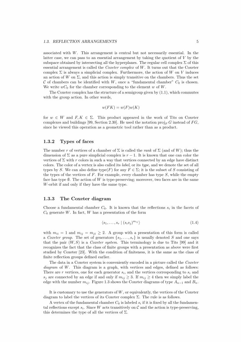
The data in a Coxeter system is conveniently encoded in a picture called the Coxeterdiagram of W . This diagram is a graph, with vertices and edges, defined as follows:There are r vertices, one for each generator si, and the vertices corresponding to si andsj are connected by an edge if and only if mij ≥ 3. If mij ≥ 4 then we simply label theedge with the number mij . Figure 1.3 shows the Coxeter diagrams of type An−1 and Bn.
It is customary to use the generators of W , or equivalently, the vertices of the Coxeterdiagram to label the vertices of its Coxeter complex Σ. The rule is as follows.
A vertex of the fundamental chamber C0 is labeled si if it is fixed by all the fundamen-tal reflections except si. Since W acts transitively on C and the action is type-preserving,this determines the type of all the vertices of Σ.

6 CHAPTER 1. COXETER GROUPS
Type An−1 : ��������s1
��������s2
. . . ��������sn−1
Type Bn : ��������s1
��������s2
. . . ��������sn−1
��������4
sn
Figure 1.3: The Coxeter diagrams of type An−1 and Bn.
1.3.4 The distance map
We write l(w) for the minimum length of w expressed as a word using elements of S.Then the gallery metric is given by
dist(uC0, vC0) = l(u−1v).
This further suggests that we can define the W -valued gallery distance function
d : C × C →W
by the formula
d(uC0, vC0) = u−1v.
It follows that this function is invariant under the diagonal action of W on C × C. Inother words,
d(C,D) = d(C′, D′) ⇐⇒ There exists a unique w such that wC = C′, wD = D′.
Also it is clear that
d(E,C) = d(E,D)d(D,C). (1.5)
The set C × C of pairs of chambers will play a central role in our theory.
1.3.5 The Bruhat order
We say that u ≤ v in the weak left Bruhat order on W if there is a minimum galleryE −D − C such that d(D,C) = u and d(E,C) = v.
Alternatively,
u ≤ v in W ⇐⇒ There is a minimum gallery v−1C0 − u−1C0 − C0.
⇐⇒ There is a minimum gallery C0 − vu−1C0 − vC0.
The first gallery condition is illustrated in Figure 1.4. The second gallery above is ob-tained from the first by multiplying by v.
u−1C0
v−1C0 C0
Figure 1.4: A minimum gallery that illustrates the partial order on W .

1.3. REFLECTION ARRANGEMENTS 7
By letting d(E,D) = w in the first definition above, one obtains a more combinatorialdescription of the weak left Bruhat order. Namely,
u ≤ v ⇐⇒ v = wu and l(v) = l(w) + l(u).
The left in the notation refers to the fact that w appears to the left of u in the expressionv = wu.
One can define the weak right Bruhat order on W , denoted ≤rb, by the equation
u ≤rb v ⇐⇒ u−1 ≤ v−1.
The partial order ≤ will be used crucially in Chapters 5, 7 and 8, while the partial order≤rb will only make a brief appearance in Chapter 7. Hence whenever we refer to thepartial order on W , it always means the weak left Bruhat order.
1.3.6 The descent algebra: A geometric approach
For a Coxeter system (W,S), let
Q = {T | T ≤ S}
be the poset of subsets of S ordered by inclusion. Let des : W → Q be the descent map
des(w) = {s ∈ S | l(ws) < l(w)}.
Let KW be the group algebra of W over the field K. Solomon [92] showed that theelements
dT =∑
des(w)≤T
w,
as T varies, give a basis for a subalgebra of KW . This subalgebra is known as the descentalgebra. Further Solomon also computed the radical of this algebra [92, Theorem 3]. Ageometric version of his result is given in Lemma 2.6.6.
Let Σ be the Coxeter complex of W and KΣ be its semigroup algebra. Let (KΣ)W
be the algebra of invariants of the W -action on KΣ. A basis for (KΣ)W is given by
σT =∑
type(F )=T
F,
as T ranges over all subsets of S. Bidigare [11] proved that the map
(KΣ)W → KW,
that sends σT to dT is an algebra anti-homomorphism. It is easy to see that this map isinjective and its image is precisely the descent algebra. Hence (KΣ)W is anti-isomorphicto the descent algebra. The proof, which is conceptual and short, is also explained inBrown [18, Section 9.6].
1.3.7 Link and join
The relevance to us of the link and join operations on simplicial complexes is that Coxetercomplexes are well behaved with respect to these operations. The facts written belowwill be crucially needed in Chapters 6, 7 and 8.

8 CHAPTER 1. COXETER GROUPS
Link
Let F ∈ Σ be a face of type T ≤ S. And let WS\T be the subgroup of W generatedby S \ T . Then the link of F in Σ, denoted link(F ), is again a Coxeter complex. TheCoxeter group of link(F ) can be viewed as a subgroup of W and it is a conjugate ofWS\T . A subgroup of W of this form is known as a parabolic subgroup. The Coxeterdiagram of link(F ) is obtained from the Coxeter diagram of Σ by deleting all the verticeswhose type is contained in T . The map
Σ→ link(F ),
that sends the face K to the face in link(F ) which corresponds to FK, is a semigrouphomomorphism. For convenience, we usually identify link(F ) with star(F ) and work withthe map Σ→ star(F ) that sends K to FK. This map also preserves opposites. Namely,if K and K are opposite faces in Σ then FK and FK are opposite faces in star(F ).
Remark It is clear that if F and F ′ are faces of the same type then link(F ) ∼= link(F ′).
Join
The join Σ1 ∗ Σ2 of two Coxeter complexes is again a Coxeter complex, whose diagramis the disjoint union of the diagrams of Σ1 and Σ2. Its Coxeter group is the cartesianproduct of the two smaller Coxeter groups. Further, the join operation is compatiblewith the projection maps and the distance map, that is,
(H1 ∗N1)(H2 ∗N2) = (H1H2 ∗N1N2), where Hi, Ni ∈ Σi.
d(C ∗ C′, D ∗D′) = (d(C,D), d(C′, D′)).
In addition, a minimum gallery in Σ1∗Σ2 yields a minimum gallery in Σ1 and a minimumgallery in Σ2. And using the galleries in the two smaller complexes, one can reconstructthe original gallery. We refer to this fact as the compatibility of galleries with joins.
1.4 The Coxeter group of type An−1
The symmetric group Sn on n letters can be generated by n − 1 transpositions s1, s2,. . ., sn−1, where si interchanges i and i+ 1 and fixes the other letters. These generatorssatisfy the relations
s2i = 1, (sisi+1)3 = 1, (sisj)
2 = 1 if i and j differ by more than 1.
This gives rise to a presentation for Sn, which is of the form written in (1.4). Hence Snis a Coxeter group, which is also known as the Coxeter group of type An−1. Its Coxeterdiagram is shown in Figure 1.3.
1.4.1 The braid arrangement
The reflection arrangement in this case is the braid arrangement in Rn. It is discussed in
detail in [11, 12, 13, 19]. It consists of the(n2
)hyperplanes Hij defined by xi = xj , where
1 ≤ i < j ≤ n. The intersection of all these hyperplanes is the line x1 = x2 = . . . = xn;so the arrangement is not essential. Each chamber is determined by an ordering of thecoordinates, so it corresponds to a permutation. The faces of a chamber are obtained bychanging to equalities some of the inequalities defining that chamber.
When n = 4, the arrangement consists of six planes in R4. By taking the quotient
of R4 by the line x1 = x2 = x3 = x4, and cutting by the unit sphere, we obtain the
spherical picture shown in Figure 1.5. It has been reproduced from Billera, Brown andDiaconis [13]. As an example, the permutation 2314 corresponds to the inequality
x2 < x3 < x1 < x4.

1.4. THE COXETER GROUP OF TYPE AN−1 9
������
����
2413 2431
2341
23142134
2143
12431234
1324 3124
3214
3412
3421
314213421432
1423
3241
1−2
2−4
2−3
3−4
1−4
1−3
Figure 1.5: The braid arrangement when n = 4.
1.4.2 Types of faces
The symmetric group Sn acts on the braid arrangement by permuting the coordinates.We fix x1 < x2 < . . . < xn to be the fundamental chamber C0. The supports of thefacets of C0 are hyperplanes of the form xi = xi+1, where 1 ≤ i ≤ n− 1. The reflectionin the hyperplane xi = xi+1 corresponds to the generator si of Sn that interchanges thecoordinates xi and xi+1. The chamber C0 has n− 1 vertices, namely
s1 : x1 < x2 = . . . = xn,
s2 : x1 = x2 < x3 = . . . = xn,...
sn−1 : x1 = . . . = xn−1 < xn.
The letters s1, s2, . . ., sn−1 on the left are labels assigned to each vertex by the rulementioned in Section 1.3.3. Applying the action of W we see, for example, that
xπ(1) < xπ(2) = . . . = xπ(n)
gives all vertices of type s1 as π varies over the permutations of [n].
1.4.3 Set compositions and partitions
A composition of the set [n] is an ordered partition F 1| . . . |F k of [n]. That is, F 1, . . . , F k
are disjoint nonempty sets whose union is [n], and their order counts. We can encode thesystem of equalities and inequalities defining a face by a composition of [n]; the equalitiesare used to define the blocks and the inequalities to order them. For example, for n = 4,
x1 = x3 < x2 = x4 ←→ 13|24.
Thus the faces of Σ are compositions of the set [n]. Observe that the vertices of type s1are two block compositions such that the first block is a singleton. Note that F is a faceof H if and only if H consists of a composition of F 1 followed by a composition of F 2,and so on, that is, if and only if H is a refinement of F .
The product in Σ is also easy to describe in this language. We multiply two com-positions by taking intersections and ordering them lexicographically; more precisely, if

10 CHAPTER 1. COXETER GROUPS
F = F 1| . . . |F l and H = H1| . . . |Hm, then
FH = (F 1 ∩H1| . . . |F 1 ∩Hm| . . . |F l ∩H1| . . . |F l ∩Hm) ,
where the hat means “delete empty intersections”. The 1-block composition is the iden-tity for the product.
The lattice of flats L is the lattice of set partitions ordered by refinement. For example,for n = 4,
x1 = x3, x2 = x4 ←→ {13, 24}.
The product or join of two set partitions is their smallest common refinement. Moreprecisely, we multiply partitions by taking intersections of the parts and deleting emptyintersections. The similarity between the product in Σ and L is explained by the supportmap. The support map Σ ։ L forgets the ordering of the blocks. For example, for n = 4,the support map sends the face 13|24 to {13, 24}.
Thus we see that set compositions and partitions emerge naturally in this example.In fact, one can explain this example in purely combinatorial terms without reference tohyperplane arrangements. More details are given in Section 5.4.
1.4.4 The Bruhat order
Let Inv(u) be the set of inversions of a permutation u ∈ Sn, that is,
Inv(u) := {(i, j) ∈ [n]× [n]∣∣ i < j and u(i) > u(j)} .
The inversion set determines the permutation. Given u and v in Sn, we write u ≤ v ifInv(u) ⊆ Inv(v). This gives the weak left Bruhat order on Sn.
Note that Inv(u) can be identified with the set of hyperplanes which separate C0 andu−1C0, by letting the pair (i, j) correspond to the hyperplane xi = xj . As an illustrativeexample, take u = 3|4|2|1. Then (1, 3) ∈ Inv(u). And note that the hyperplane x1 = x3
separatesx1 < x2 < x3 < x4 and x4 < x3 < x1 < x2,
which are the chambers C0 and u−1C0 respectively. Now using (1.3), one sees that theabove definition of the weak left Bruhat order is same as the gallery definition givenearlier.
3214 3142 2413 23414123 1432
3124 2143 1423 13422314
1324 1243
4213 4132 3412 24313241
4312 3421
1234
2134
4321
4231
Figure 1.6: The weak left Bruhat order on S4.
Figure 1.6, which is taken from [4], shows the partial order on S4. It can also bedrawn from Figure 1.5 by replacing each permutation by its inverse and drawing an edgebetween adjacent chambers.

Chapter 2
Left regular bands
Left regular bands, or LRBs for short, are semigroups that have been of recent interestin random walk theory. They are easy to define and work with and have a rich source ofexamples. For more details, see the seminal paper of Brown [18]. The main example is theposet of faces of a hyperplane arrangement defined in Section 1.2. The LRB terminologywe use is motivated by this example. Coxeter complexes fall in this category as theyarise from reflection arrangements. As a slightly more general example, we have theposet of covectors of an oriented matroid. More information about LRBs can be found inGrillet [38] and Petrich [76, 77]. The origin of LRBs can be traced to Schutzenberger [90].
2.1 Why LRBs?
The main motivation for LRBs is that many of our results in Chapter 5 generalize toLRBs. Coxeter complexes, and more generally, the poset of faces of a hyperplane ar-rangement, to which most of the theory is applied, can be viewed as special cases. Toeffect this generalization, one is forced to develop the standard theory of LRBs further.We begin with the standard material in Section 2.2 and then present the new materialin Sections 2.3-2.7.
In Section 2.3, we introduce the concept of a pointed face. This notion will allow usto properly formulate the adjointness properties of the descent map to be considered inChapter 5. Similarly, Section 2.4 on sub and quotient LRBs is motivated by the Hopfalgebra considerations in Chapter 6.
In Section 2.5, we define and study a bilinear form on any LRB Σ. This bilinearform controls the commutativity in diagram (5.8), which we will encounter in Chapter 5.We show that the radical of this form contains the radical of the semigroup algebra KΣ,which was computed by Bidigare [11] and Brown [18]. Further we give a computablecriterion for the equality of radicals to hold.
In Section 2.6, we specialize to the case when Σ is the Coxeter complex of a Coxetergroup. In this situation, one can pass to invariants and induce a bilinear form on (KΣ)W ,which can be identified with KQ defined in Section 1.3.6. We know that (KΣ)W is anti-isomorphic to the descent algebra (Section 1.3.6). Following the method in Section 2.5,we show that the radical of the above form contains the radical of the descent algebra.Further we show that the two radicals are equal if the above mentioned criterion issatisfied.
Some of our results in the second part of Chapter 5 generalize further to projectionposets, which is a notion that we introduce in Section 2.7. This allows us to considernonassociative structures like buildings and modular lattices.
11

12 CHAPTER 2. LEFT REGULAR BANDS
2.2 Faces and flats
The material in this section is taken from Brown [18, Appendix B]. In this section andthe next, we define the basic objects related to LRBs. Towards the end of each section,we explain the examples of a hyperplane arrangement and the free LRB. The example ofthe braid arrangement is explicitly worked out in Sections 1.4 and 5.4. The reader maywant to read these sections in parallel with the material below.
2.2.1 Faces
Let Σ be a left-regular band, or a LRB for short. It is a semigroup that satisfies theidentities
x2 = x and xyx = xy (2.1)
for all x, y ∈ Σ. Early references to this concept occur in Klein-Barmen [50] andSchutzenberger [90]. For simplicity, we assume that Σ is finite and has a unit. In thiscase, the first identity follows from the second.
The relationx ≤ y ⇐⇒ xy = y
defines a partial order on Σ. Elements of Σ are called faces and for x ≤ y, one says thatx is a face of y.
• If x ≤ y then zx ≤ zy for any z; however, xz ≤ yz may not hold.
• If there is z such that xz = y then x ≤ y. In other words, x is always a face of xz.
The above properties follow from the definitions. A complete list of properties whichwe will need to use later is given in Section 2.7.2.
2.2.2 Flats
Define another relation � on Σ by x � y ⇐⇒ yx = y. This is transitive and reflexive,but not necessarily antisymmetric. We therefore obtain a poset L by identifying x and yif x � y and y � x. We denote the quotient map by supp: Σ ։ L. Then
yx = y ⇐⇒ suppx ≤ supp y
holds by definition. Elements of L are called flats. It follows that
xy = x and yx = y ⇐⇒ suppx = supp y. (2.2)
The support map is order preserving. To see this, suppose that x ≤ y, that is, xy = y.Premultiplying by y and using Equation (2.1), we conclude that yx = y and hencesuppx ≤ supp y. Following [18, Appendix B], it can also be shown that L is a joinsemilattice and that
suppxy = suppx ∨ supp y. (2.3)
In other words, the support map is a map of semigroups, with the product in L given bythe join.
2.2.3 Chambers
We call an element c ∈ Σ a chamber if supp c = 1, where 1 is the largest element of L.
Proposition 2.2.1 [18, Proposition 9] The following conditions on an element c ∈ Σare equivalent:

2.3. POINTED FACES AND LUNES 13
1. c is a chamber.
2. cx = c for all x ∈ Σ.
3. c is maximal in the poset Σ.
For a partial generalization, see Lemma 2.7.6. Thus the set C of chambers consistsof the maximal elements of Σ and is a two sided ideal in Σ. Let Cx = {c ∈ C | x ≤ c}.Observe the following.
Lemma 2.2.1 If xy = x and yx = y then there is a bijection Cx → Cy given by c 7→ yc
and with inverse d 7→ xd.
For a generalization of this result to projection posets, see Lemma 2.7.7.
2.2.4 Examples
Example The motivating example of a LRB is the poset of faces of a central hyperplanearrangement, with the product as given in (1.1). The notion of flats and the supportmap given by the LRB theory agree with those described in Section 1.2. The reader maycompare Equations (2.3) and (1.2).
Example The free LRB on n letters consists of words with no letter repetitions. Theproduct of u and v is the concatenation (uv) , where the hat means “delete the letters inv that have occurred in u”. The empty word is the identity for this product. And u ≤ vif u is an initial subword of v. The chambers are the permutations of the n letters. Thelattice of flats consists of subsets of the n letters, and the support map sends a word tothe subset of letters it contains.
2.3 Pointed faces and lunes
There is an analogue of Sections 2.2.1 and 2.2.2 with faces and flats replaced by pointedfaces and lunes respectively. Details are as below.
2.3.1 Pointed faces
Let Q = {(x, c) | x ≤ c} ⊆ Σ× C. Define a partial order on Q by
(x, c) ≤ (y, d) ⇐⇒ c = d and x ≤ y.
Elements of Q are called pointed faces.
2.3.2 Lunes
Define another relation � on Q by (x, c) � (y, d) ⇐⇒ yx = y and yc = d. This istransitive and reflexive, but not necessarily antisymmetric. We therefore obtain a posetZ by identifying (x, c) and (y, d) if (x, c) � (y, d) and (y, d) � (x, c). We denote thequotient map by lune: Q ։ Z. Then
yx = y and yc = d ⇐⇒ lune(x, c) ≤ lune(y, d)
holds by definition. Elements of Z are called lunes and lune(x, c) is called the lune of xand c. It follows that
xy = x, xd = c, yx = y and yc = d ⇐⇒ lune(x, c) = lune(y, d). (2.4)
The lune map is order preserving. To see this, suppose that (x, c) ≤ (y, c), that is, xy = y.Argue as for the support map to conclude that yx = y and hence lune(x, c) ≤ lune(y, c).

14 CHAPTER 2. LEFT REGULAR BANDS
2.3.3 The relation of Q and Z with Σ and L
For a poset P , let KP be the vector space over K with basis the elements of P . Note thatKΣ and KL are semigroup algebras. The relation of Q and Z with Σ and L respectivelycan be seen as follows. Define the map base : Q → Σ by (x, c) 7→ x and the mapbase∗ : KΣ → KQ by x 7→
∑c: x≤c
(x, c). These maps induce maps Z → L and KL → KZ
so that the following diagrams commute.
Σ
supp
����
Qbaseoo
lune
����L Z
baseoo
KΣ� � base∗ //
supp
����
KQ
lune
����KL
base∗//KZ
(2.5)
Proof For the first diagram, we need to show that
lune(x, c) = lune(y, d) =⇒ suppx = supp y.
This follows from (2.2) and (2.4).For the second diagram, we need to show that
suppx = supp y =⇒∑
c∈Cx
lune(x, c) =∑
d∈Cy
lune(y, d).
This follows from (2.2), (2.4) and Lemma 2.2.1.�
2.3.4 Lunar regions
There is another approach one can take to lunes, which is closer to intuition and whichjustifies the terminology. Namely, define a map reg : Q→ {R | R ⊆ Σ} by
reg(x, c) = {y | xy ≤ c}. (2.6)
The terminology R and reg(x, c) indicate that these are “regions” in Σ. We say thatreg(x, c) is the lunar region of x and c in Σ. Let Z′ be the image of the map reg. Thesets Z′ and Z are closely related; the precise relation between them is as follows.
Lemma 2.3.1 There is a commutative diagram
Qlune
��������
� reg
�� ��???
??
Z zone// // Z′
Equivalently, by (2.4), for x ≤ c and y ≤ d, we have
xy = x, xd = c, yx = y and yc = d =⇒ reg(x, c) = reg(y, d). (2.7)
We call the induced map Z→ Z′ the zone map.
Proof Let x, y, c, d be as in the left hand side of (2.7). Now let z ∈ reg(x, c), that is,xzc = c. Then
yzd = yxzyc = yxzc = yc = d.
For the first equality, we used y = yx and d = yc. For the second equality, we usedEquation (2.1). From the above equation, we conclude that z ∈ reg(y, d). This showsthat reg(x, c) ⊆ reg(y, d) and the result follows by symmetry.
�

2.3. POINTED FACES AND LUNES 15
Open Question Identify the class of LRBs for which the zone map is a bijection; inother words, for which the reverse implication in (2.7) holds.
We give a partial answer to this question. The zone map is a bijection for the posetof faces of hyperplane arrangements, see Lemma 2.3.3. However, this fails for the freeLRB, see Section 2.3.5. In the general case, one can say the following.
reg(x, c) = reg(y, d) =⇒ reg(x, c) = reg(xy, c) = reg(y, d) = reg(yx, d). (2.8)
Note that reg(x, c) = reg(y, d) implies that y ∈ reg(x, c), that is, xy ≤ c. Hence the termreg(xy, c) written above makes sense.
Proof By symmetry, it is enough to show that reg(x, c) = reg(xy, c). This follows bythe following string of equivalences.
z ∈ reg(xy, c) ⇐⇒ xyz ≤ c ⇐⇒ yz ∈ reg(x, c) ⇐⇒ yz ∈ reg(y, d)
yz ∈ reg(y, d) ⇐⇒ yyz ≤ d ⇐⇒ z ∈ reg(y, d) ⇐⇒ z ∈ reg(x, c)
The third and last equivalence hold by the assumption reg(x, c) = reg(y, d) and the resthold by the definition of a lunar region given in (2.6).
�
2.3.5 Examples
Example We return to the example of hyperplane arrangements and first describe theset of lunar regions Z′. More material on lunes can be found in Billera, Brown andDiaconis [13] or Mahajan [60, Chapter 1]. Just as an element of L is an intersection ofhyperplanes, an element of Z′ is an intersection of a special set of closed half-spaces.
Lemma 2.3.2 The lunar region of F and D, namely reg(F,D), is the intersection ofthose closed half-spaces which contain D and whose supporting hyperplane contains F .More precisely, reg(F,D) consists of those faces which lie in the above intersection.
Proof Using (1.1), we obtain:
FK ≤ D ⇐⇒If a hyperplane H contains F then itdoes not separate K and D.
The lemma now follows from the definition of a lunar region given in (2.6).
Remark We note that reg(F,D) is a chamber in the subarrangement consisting ofthose hyperplanes which contain F . The walls of this chamber are same as the wallsof D which contain F . This requires an extra argument which we leave to the reader.Hence reg(F,D) is in fact the intersection of those closed half-spaces which contain D
and whose supporting hyperplane contains F and is a wall of D.
Remark In the lemma below, we will identify lunes and lunar regions. Hence we maysay that the base of the lunar region reg(F,D) is suppF .
In Figure 2.1, we have shown two schematic spherical pictures for lunar regions in arank 3 arrangement. Note that hyperplanes in this case are great circles on the sphere.In the first picture, F is a vertex of the two dimensional chamber D; hence there are twosupporting hyperplanes in question. The two great circles intersect at F and its oppositevertex P , dividing the sphere into four regions. The region containing D is the lunarregion reg(F,D) and its base consists of the two vertices F and P .
In the second picture, F is an edge; hence there is only one supporting hyperplanein question. It divides the sphere into two regions. The region containing D is the lunar

16 CHAPTER 2. LEFT REGULAR BANDS
P
P
F
F
C
C
D
D
Figure 2.1: Two low dimensional pictures of the lunar regions reg(P,C) = reg(F,D).
region reg(F,D) and its base is the hyperplane itself, which is shown as the ellipse passingthrough F and P . For a more concrete example of a lunar region, see the shaded regionin Figure 7.2.
Lemma 2.3.3 For the poset of faces of a central hyperplane arrangement, the zone mapZ→ Z′ in Lemma 2.3.1 is a bijection.
Proof By (2.7) and (2.8), it is enough to show that
reg(F,D) = reg(FP,D) =⇒ F = FP,
where F and P are arbitrary faces with P ∈ reg(F,D).
Let reg(F,D) = reg(FP,D) and P be the opposite face to P . Since PP = P , we haveFPP = FP ≤ D. Hence by definition P ∈ reg(FP,D), which by assumption impliesP ∈ reg(F,D). Therefore we obtain FP, FP ≤ D. By applying the third elementaryproperty of the product listed in Section 1.2.1, we conclude that FP = FP = F .
�
Remark As one can see from the proof, the existence of an opposite makes centralhyperplane arrangements special among LRBs.
Example We return to the example of the free LRB on n letters. From the definition,we have lune(x, c) = lune(y, d) if x and y contain the same letters and the subword ofc obtained by deleting the initial segment x is same as the subword of d obtained bydeleting the initial segment y. Thus the set Z can be identified with the set of words inthe n letters without repetition, which is the same as Σ. The lune map then sends thepointed face (x, c) to the subword of c obtained by deleting the initial segment x. In thisnotation, a word y is an element of zone(x) if the letters which are common to both x
and y form an initial segment of x. In particular, the zone of a one letter word is theentire set Σ. This shows that the zone map is not injective. To give a concrete example,take n = 3 and the letters to be x, y and z. Then
reg(xy, xyz) = reg(yz, yzx) but lune(xy, xyz) 6= lune(yz, yzx),
which says that zone(z) = zone(x).
2.4 Link and join of LRBs
In Chapter 6, we will construct Hopf algebras from the family of LRBs {Σn}n≥0, whereΣn is the Coxeter complex of Sn. In this section, we state two simple but useful lemmasin the construction. They are valid for any LRB.

2.5. BILINEAR FORMS RELATED TO A LRB 17
2.4.1 SubLRB and quotient LRB
Let Σ be a LRB and Q, L and Z be as above. Let
Σx = {y ∈ Σ | x ≤ y}.
Then Σx is a LRB in its own right, which we may also call the link or star region of x inΣ. Denote its corresponding objects by Qx, Lx and Zx respectively. Explicitly, we have
Qx = {(y, d) ∈ Q | x ≤ y ≤ d},
Lx = {X ∈ L | suppx ≤ X}, and
Zx = {lune(y, d) ∈ Z | x ≤ y ≤ d} = {L ∈ Z | suppx ≤ baseL}.
In addition to a subLRB, one can view Σx as a quotient LRB of Σ. The quotient map
x· : Σ ։ Σx
sends y to xy. This induces the map x· : Q ։ Qx which sends (y, d) to (xy, xd), themap x· : L ։ Lx which sends X to X ∨ suppx, and the map x· : Z ։ Zx which sendslune(y, d) to lune(xy, xd).
Lemma 2.4.1 The following diagrams commute.
Σx� � //
supp
����
Σx· // //
supp
����
Σx
supp
����Lx
� � // L x·// // Lx
Qx� � //
lune
����
Qx· // //
lune
����
Qx
lune
����Zx
� � // Z x·// // Zx
The proof is a direct consequence of the definitions.
2.4.2 Product of LRBs
For i = 1, 2, let Σi be a LRB and Qi, Li and Zi be the associated objects. Then thecartesian product Σ = Σ1 × Σ2 is a LRB with componentwise multiplication; we maycall Σ the join of Σ1 and Σ2.
Lemma 2.4.2 The associated posets of Σ = Σ1×Σ2 are Q = Q1×Q2, L = L1×L2 andZ = Z1 × Z2.
2.5 Bilinear forms related to a LRB
In this section, we initiate a study of three bilinear forms related to a LRB. They aredefined on KQ, KΣ and KL respectively. The material in Sections 2.5.1-2.5.3, exceptLemma 2.5.1 and Corollary 2.5.1, generalizes to projection posets, which are defined inSection 2.7.
2.5.1 The bilinear form on KQ
Define a symmetric bilinear form on KQ by
〈(x, c), (y, d)〉 =
1if yc = d and xd = c, or equivalently,if c ∈ reg(y, d) and d ∈ reg(x, c),
0 otherwise.

18 CHAPTER 2. LEFT REGULAR BANDS
In Figure 2.2, we have shown the schematic picture of two intersecting lunar regions.It illustrates the case when 〈(P,C), (F,D)〉 = 1 for the poset of faces of a hyperplanearrangement.
PF
CD
Figure 2.2: The pointed faces (P,C) and (F,D) lie in each other’s lunar regions.
Open Question The above form is degenerate in general. Compute its radical.
As a partial answer, we give one source of degeneracy in the Coxeter case. In thiscase, by passing to invariants, we obtain an induced form on (KQ)W ∼= KQ, which weshow to be degenerate in Section 2.6. This implies by general principles that the originalform was also degenerate. For example, for T, U ≤ S, if T − U is in the radical of theinduced form then ∑
D∈C
(TD, D)− (UD, D) (2.9)
belongs to the radical of the original form. Here TD refers to the face of D which is oftype T .
Example For type A, the elements of Σ and Q are set compositions and fully nestedset compositions respectively, see Section 5.4. One can give an explicit combinatorialdefinition for the bilinear form on KQ. We illustrate it by the following example.
〈(6|2|3|5|1|4|7), (4|6|7|2|5|1|3)〉 = 1.
This is because 6|2|3|5|1|4|7 is a shuffle of 4, 6|7, 2|5|1, 3 and 4|6|7|2|5|1|3 is a shuffle of6|2|3, 5|1, 4|7. This should make the general definition clear. The reader can also playwith Figure 1.5 and match the geometric and combinatorial definitions for n = 4.
To obtain an element in the radical of this form, one can take T and U to be twocompositions, say (1, 2, 1) and (2, 1, 1), with the same underlying partition, and then useformula (2.9).
2.5.2 The pairing between KQ and KΣ
Consider the diagram
KQ×KΣ))SSSS
KΣ×KΣ
55kkkk
))SSSS KQ×KQ // K,
KΣ×KQ
55kkkk(2.10)
induced by the map base∗ : KΣ → KQ given by x 7→∑
c: x≤c(x, c). The rightmost map is
the bilinear form defined in Section 2.5.1.

2.5. BILINEAR FORMS RELATED TO A LRB 19
Explicitly, the map KQ×KΣ→ K is given by
〈(x, c), y〉 =
{1 if xyc = c, or equivalently, y ∈ reg(x, c),
0 otherwise.
From the definition of the map reg : Q→ Z′, we have the following.
Lemma 2.5.1 The kernel of the map reg : KQ→ KZ′ lies in the left radical of the mapKQ×KΣ→ K. Hence there is a commutative diagram
KQ×KΣ
��
**UUUUUUU
K
KZ′ ×KΣ
44iiiiiii
2.5.3 The bilinear form on KΣ
Note that diagram (2.10) defines a symmetric bilinear form on KΣ. It is given by
〈x, y〉Σ = |{(c, d) | xd = c, yc = d}|. (2.11)
There is an alternate way to define this bilinear form. For each x ∈ Σ, let cx = |Cx| bethe number of chambers c ∈ C such that c ≥ x. Define a linear map ζ : KΣ→ K by
ζ(x) = cx. (2.12)
Lemma 2.5.2 We have 〈x, y〉Σ = ζ(xy).
Proof Since supp(xy) = supp(yx), by Lemma 2.2.1, there is a bijection
bij : Cxy → Cyx
given by c 7→ yxc with inverse d 7→ xyd.Let (C × C)x,y = {(c, d) | yc = d, xd = c}. Then
(c, d) ∈ (C × C)x,y ⇐⇒ c ∈ Cxy, d ∈ Cyx, bij(c) = d.
To see the forward implication, note that (c, d) ∈ (C × C)x,y implies y ≤ d and x ≤ c.Hence yc = y(xc) = d. This says that yx ≤ d and bij(c) = d. Similarly xy ≤ c. Thebackward implication is similar. This proves the lemma.
�
Corollary 2.5.1 The form 〈 , 〉Σ on KΣ is invariant. In other words,
〈x, yz〉Σ = 〈xy, z〉Σ.
2.5.4 The bilinear form on KL
The bilinear form on KΣ is far from being nondegenerate. We know from Lemma 2.2.1that cx depends only on suppx. Hence for each X ∈ L, let cX be the number of chambersc ∈ C such that c ≥ x, where x is any fixed element of Σ having support X . The map ζfactors through KL giving a function ζ : KL→ K with
ζ(X) = cX . (2.13)
Now 〈x, y〉Σ = ζ(xy) = ζ(supp xy) = ζ(supp x ∨ supp y). This shows the following.

20 CHAPTER 2. LEFT REGULAR BANDS
Lemma 2.5.3 The form 〈 , 〉Σ : KΣ×KΣ→ K and the map ζ : KΣ→ K factor throughKL to give a form 〈 , 〉L : KL×KL→ K and a map ζ : KL→ K satisfying
〈X,Y 〉L = ζ(X ∨ Y ).
In other words, there are two commutative diagrams
KΣ×KΣ
supp× supp
��
**UUUUUUUUUU
K
KL×KL
44iiiiiiiiii
KΣ
supp
��
ζ
))SSSSSSSSS
K
KLζ
55kkkkkkkkk
2.5.5 The nondegeneracy of the form on KL
Now we discuss conditions under which the induced form 〈 , 〉L on KL is nondegenerate.
Definition 2.5.1 We define numbers nX by the equation
∑
X≤Y
nY = cX ,
for each X ∈ L. Equivalently, nX =∑X≤Y µ(X,Y )cY , where µ is the Mobius function
of the lattice L.
The numbers nX , in this generality, were defined by Brown. They are the genericmultiplicities of certain random walks on the chambers of a LRB, see [18, Theorem 1].For the special case of hyperplane arrangements, nX = |µ(X, 1)|, where 1 is the maximumelement of L and µ is its Mobius function. This follows from a formula of Zaslavsky [101].The connection of these numbers to random walks was first made by Bidigare, Hanlonand Rockmore [11, 12].
Lemma 2.5.4 The semigroup algebra KL is split semisimple, that is, it is isomorphicto a product of copies of K. Further, the form 〈 , 〉L : KL× KL → K is nondegenerate⇐⇒ nX 6= 0 for each X ∈ L.
The first part is due to Solomon [91], see also Greene [37] and Stanley [93, Section 3.9].It holds for any finite semilattice.
Proof Explicitly, for the first part, if KL denotes the algebra of functions from L to K,
then there is an algebra isomorphism KL∼=−→ K
L given by X 7→∑X≤Y δY , where δY is
defined to be 1 at Y and 0 elsewhere.For the second part, let qX be the element of KL, which corresponds to δX under this
isomorphism. Then qX are the orthogonal idempotents for the algebra KL. It followsfrom Definition 2.5.1 that ζ(qX) = nX . We now compute the form 〈 , 〉L on the {qX}basis.
〈qX , qY 〉L = ζ(qXqY ) = ζ(qX)δX,Y = nXδX,Y , (2.14)
where δX,Y denotes the Kronecker delta. The result follows.�
Lemma 2.5.5 The kernel of the support map KΣ → KL is rad(KΣ), where rad(KΣ)stands for the Jacobson radical of KΣ.
This result is due to Bidigare and Brown.

2.6. BILINEAR FORMS RELATED TO A COXETER GROUP 21
Proof Bidigare [11] showed that for Σ arising from hyperplane arrangements, the kernelof the support map KΣ→ KL is nilpotent. And since KL is semisimple, the result follows.The same proof was generalized to LRBs by Brown [18, Section 7.2].
�
Corollary 2.5.2 We have nX 6= 0 for each X ∈ L ⇐⇒ rad〈 , 〉Σ = rad(KΣ).
This follows from the previous two lemmas and gives a computable criterion to checkequality of the radicals.
Open Question Identify the class of LRBs for which the above criterion holds.
It is known that the above criterion holds for Σ arising from hyperplane arrangements;see Orlik and Terao [71, Theorem 2.47]. We thank Victor Reiner for this reference.However one can check that the criterion fails for the free LRB. The reader who hascome this far may be convinced that free LRBs are good for producing counterexamples.
Example We recall that for type A, the elements of Σ and L are set compositions andset partitions respectively.
If F = F 1|F 2| . . . |F k is a set composition then cF = f1!f2! . . . fk! where fi = |F i|.Note that this depends only on the cardinalities of the F i and not on their order. Inother words, cF only depends on suppF = {F 1, F 2, . . . , F k}, as expected.
Using the formula for the Mobius function of the poset of set partitions, we obtain:
nX = |µ(X, 1)| = (x1 − 1)! . . . (xk − 1)!, (2.15)
where X = {X1, X2, . . . , Xk} and xi = |X i|. Note that nX 6= 0 for each X ∈ L, asalready claimed above.
Remark In the Coxeter case, the numbers nX are related to the invariant theory ofthe Coxeter group W . If X is the minimum element of L, then nX = |µ(X, 1)| is theproduct of the exponents of W , and hence in particular is nonzero. This is an old resultof Orlik and Solomon [70], see also Orlik and Terao [71, Corollary 6.62]. For any otherelement X in the lattice, the interval [X, 1] is isomorphic to the intersection lattice foranother Coxeter group W ′, which is a parabolic subgroup of W ; hence the above resultapplies.
2.6 Bilinear forms related to a Coxeter group
Let (W,S) be a Coxeter system and Σ be the Coxeter complex of W . Then the diagram
KQ ∼= (KΣ)W
supp
����
� � //KΣ
supp
����KL ∼= (KL)W
� � //KL
commutes. In Section 2.5, we studied bilinear forms on KQ, KΣ and KL for any LRBΣ. In the setting of Coxeter groups, it is clear that these forms are invariant under theW -action, and hence induce symmetric bilinear forms on KQ ∼= (KQ)W ∼= (KΣ)W andKL ∼= (KL)W . In this section, we study these two induced bilinear forms.
We have encountered the object Q in the context of the descent algebra (Section 1.3.6).The object L is new; it is defined as the set of W -orbits in L. In fact, it has a partialorder which it inherits from L.

22 CHAPTER 2. LEFT REGULAR BANDS
2.6.1 The bilinear form on (KΣ)W
In this subsection, we give some interesting descriptions of the bilinear form on (KΣ)W .We recall that a basis for (KΣ)W is given by
σT =∑
type(F )=T
F,
as T ranges over all subsets of S.
Lemma 2.6.1 We have
1
|W |〈σT , σU 〉 = |{w ∈ W | des(w) ≤ T, des(w−1) ≤ U}|.
Compare this equation with [4, Proposition 9.4].
Proof Consider the set
(C × C)T,U = {(C,D) | TCD = C and UDC = D},
where TC is the face of C of type T , and UD is the face of D of type U . It is clear thatthis set is closed under the diagonal action of W on C × C. From (2.11), we see that theleft hand side of the above equation counts the number of W -orbits in this set. Furthernote that each W -orbit can be indexed by an element w ∈W using the rule d(C,D) = w.Hence one has to determine those w ∈ W , which occur as orbits in (C × C)T,U . This isdone by translating the condition on the projection maps into a condition on des(w) anddes(w−1). This will be the content of Proposition 5.3.2. This gives the right hand sideof the above equation.
�
Using Lemma 2.5.2, the bilinear form on (KΣ)W can be written as
〈σT , σU 〉 = ζ(σTσU ), (2.16)
where ζ is given by (2.12). Now write
σTσU =∑
V≤S
αVTUσV .
Since (KΣ)W is anti-isomorphic to the descent algebra, the constants αVTU may alsobe regarded as the structure constants of the descent algebra (Section 1.3.6). We nowdescribe the bilinear form using these constants.
Lemma 2.6.2 We have 〈σT , σU 〉 = |W |∑V≤S
αVTU .
Proof Using the above equations, we have 〈σT , σU 〉 =∑V≤S
αVTUζ(σV ). It remains to
show thatζ(σV ) = |W | for all V ≤ S.
The left hand side counts pairs (F,D) with F ≤ D and typeF = V . Since every chamberhas a unique face of type V , this is same as the number of chambers, which is |W |.
�
Lemma 2.6.3 Let F ≤ H and typeF = T and typeH = V . Then αVTU counts thenumber of faces N of type U such that FN = H.

2.6. BILINEAR FORMS RELATED TO A COXETER GROUP 23
This lemma follows from the definition. Combining Lemmas 2.6.2 and 2.6.3 gives usthe following description.
Lemma 2.6.4 Let F ≤ D and typeF = T . Then
1
|W |〈σT , σU 〉 = |{N ∈ reg(F,D) | typeN = U}|.
Note that the symmetry of the bilinear form is not at all clear from the right handside. Hence we can use the symmetry along with this lemma to derive a nontrivial resultabout lunar regions as follows.
Corollary 2.6.1 The number of faces of type U in Σ, say fU , is equal to the number ofchambers in the lunar region reg(F,D), where F is any face of type U and F ≤ D.
This result is also implied by Mahajan [60, Lemma 5].
Proof Recall that S is the set of reflections and any chamber D is of type S. By thesymmetry of the bilinear form on (KΣ)W , we have
1
|W |〈σS , σU 〉 =
1
|W |〈σU , σS〉.
Now use Lemma 2.6.4 on both sides. Note that reg(D,D) = Σ. Hence the left hand sideis the number of faces of type U in Σ. And the right hand side is the number of chambersin the lunar region reg(F,D), where F is any face of type U and F ≤ D.
�
2.6.2 The bilinear form on (KL)W and its nondegeneracy
It is clear that the bilinear form on (KΣ)W factors through the map (KΣ)W → (KL)W
to give a bilinear form 〈 , 〉 : (KL)W × (KL)W → K. In analogy with Lemma 2.5.4, onecan show:
Lemma 2.6.5 The algebra (KL)W is split semisimple. Further, the form 〈 , 〉 : (KL)W×(KL)W → K is nondegenerate ⇐⇒ nX 6= 0 for each X ∈ L.
The proof is straightforward and is given in Lemma 5.7.1. The main step is toconstruct a basis for (KL)W such that each basis element when viewed as an element ofKL is a sum of primitive idempotents.
Lemma 2.6.6 The kernel of the support map (KΣ)W → (KL)W is rad((KΣ)W ).
Proof The kernel is nilpotent because it sits inside rad(KΣ) which is nilpotent. Andsince (KL)W is semisimple, the result follows.
�
The above result (phrased in a different language) was obtained by Solomon [92,Theorem 3]. For other proofs and additional related results, see Atkinson [6], Garsia andReutenauer [32] and Krob, Leclerc and Thibon [51, Corollary 3.11]. A lift of the theprimitive idempotents of (KL)W to (KΣ)W is given by Bergeron, Bergeron, Howlett andTaylor [7]. For a recent survey on the descent algebra, see Schocker [89].
The previous two lemmas give us the following corollary relating the radical of thedescent algebra to the radical of the bilinear form on it.
Corollary 2.6.2 We have nX 6= 0 for each X ∈ L ⇐⇒ rad〈 , 〉(KΣ)W = rad((KΣ)W ).
Note that the criterion for the equality of the radicals in the coinvariant case is thesame as the criterion obtained in Corollary 2.5.2.

24 CHAPTER 2. LEFT REGULAR BANDS
2.7 Projection posets
In this section, we introduce projection posets, which are more general than LRBs.The main motivation is that some of our results hold in this generality. However, theconstructions of the objects L and Z are specific to LRBs; they do not generalize toprojection posets.
2.7.1 Definition and examples
Definition 2.7.1 A projection poset Σ is a poset with a (not necessarily associative)product Σ× Σ→ Σ that satisfies:
(1) The product x1x2 . . . xn is well-defined if there exist y, z such that for every 1 ≤i ≤ n, either xi ≤ y or xi ≤ z.
(2) y2 = y and yzy = yz.
(3) yz = z ⇐⇒ y ≤ z.
(4) The set of chambers (maximal elements) C is a left ideal in Σ.
Proposition 2.7.1 Every LRB is a projection poset.
Proof Since the product in a LRB is associative, x1x2 . . . xn is always well-defined; so(1) holds. Property (2) holds by definition. The next two properties are a part of LRBfoundations, which were discussed in Section 2.2. Note that the definition of a LRB doesnot involve any poset. The point is to first define a relation on a LRB using property (3)and then to prove that it is a partial order.
�
A projection poset is not an empty generalization of a LRB. The generalization doesindeed give new examples.
Proposition 2.7.2 The poset of faces of a building and the order complex of a modularlattice are projection posets.
Proof A building is a simplicial complex obtained by gluing together Coxeter com-plexes. These Coxeter complexes are called the apartments of the building. For a building∆, given y, z ∈ ∆, one can always choose an apartment containing y and z. Details canbe found in Brown [17]. Tits defined a product (not necessarily associative) on the posetof faces of a building [99, Section 3.19]. One way to describe the product yz is to firstchoose an apartment containing y and z, and then take the product in that apartment.
Readers may now readily see the origin of property (1). Namely, one can choose anapartment containing the elements x1, x2, . . . , xn. The product x1x2 . . . xn is then well-defined because the product within an apartment is associative. Similarly, buildings alsosatisfy properties (2)− (4). All of them involve at most two distinct elements, hence onecan always choose an apartment containing them and argue as above.
In [1], Abels showed that the order complex of any modular lattice behaves like thebuilding of type A. The role of apartments is played by distributive lattices. The ordercomplex of a distributive lattice corresponds to a convex set of chambers in the braidarrangement [1, Proposition 2.5]. Hence it is an example of a LRB; in particular, itsproduct is associative. The same argument as for buildings then shows that the ordercomplex of a modular lattice is a projection poset.
�
The examples in the proposition above were referred to as nonassociative LRBs inMahajan [60, Chapter 1], where related material can be found.

2.7. PROJECTION POSETS 25
2.7.2 Elementary facts
We now generalize some known facts about LRBs to projection posets. These facts,though elementary, are important. They will allow us to use projection posets as thebasis for an axiomatic treatment of Hopf algebras in Chapter 6.
Lemma 2.7.1 We have y ≤ yz.
Proof By property (1), we know that yyz is well-defined. By property (2), we havey2 = y; hence y(yz) = (yy)z = yz. Now, applying property (3), we obtain y ≤ yz.
�
Lemma 2.7.2 If y ≤ z then zy = z.
Proof Let y ≤ z. Then by property (3), we have yz = z. Premultiplying by z, we getzyz = z2. Property (3) now implies that zy = z.
�
Lemma 2.7.3 If x ≤ y ≤ z and xw = z then yw = z.
Proof This follows from the sequence of equalities yw = yxw = yz = z. The firstequality uses Lemma 2.7.2.
�
Lemma 2.7.4 An element ∅ is the identity in Σ if and only if ∅ is the unique minimalelement in Σ.
Proof From property (3), we have
∅x = x for all x ⇐⇒ ∅ ≤ x for all x.
Also by Lemma 2.7.2, if ∅ ≤ x for all x then x∅ = x for all x.�
Lemma 2.7.5 If y ≤ z then xy ≤ xz.
Proof Let y ≤ z. Then xyxz is well-defined by property (1). By properties (2) and(3), we have xyxz = xyz = xz. Therefore, we get xy(xz) = xz, which by property (3)says that xy ≤ xz.
�
The set of chambers C in Σ can also be characterized using the product in Σ as below,also see Proposition 2.2.1.
Lemma 2.7.6 We have that c is a chamber in Σ ⇐⇒ cx = c for all x ∈ Σ.
Proof For the forward implication, note by Lemma 2.7.1 that c ≤ cx for all x, c ∈ Σ;so if c is maximal then c = cx for all x ∈ Σ. Conversely, if cx = c for all x ∈ Σ then c ismaximal because c ≤ x =⇒ cx = x =⇒ c = x.
�
Let Cx = {c ∈ C | x ≤ c}. The following is a generalization of Lemma 2.2.1.
Lemma 2.7.7 If xy = x and yx = y then there is a bijection Cx → Cy given by c 7→ yc
and with inverse d 7→ xd.

26 CHAPTER 2. LEFT REGULAR BANDS
Proof By property (4), we know that the maps in the lemma are well-defined. We wantto show that they are inverse to each other. By symmetry, it is enough to show that forx ≤ c, we have x(yc) = c. By property (1), we know that xyc is well-defined. Further,from assumption and property (3), we get xyc = xc = c.
�
Corollary 2.7.1 There is a bijection Cxy → Cyx given by c 7→ yxc with inverse d 7→ xyd.
Proof By property (1), we know that yxxy is well-defined and by property (2), we haveyxxy = yx. Similarly, we have xyyx = xy. The assertion now follows from the previouslemma.
�
Lemma 2.7.8 Let y ≤ z. Then
xz ≤ c ⇐⇒ xy ≤ c and yxz ≤ yc.
This result will be crucially used in Chapter 6, see the corollary to Proposition 6.4.5. Ifz is a chamber, say d, then we may say
xd = c ⇐⇒ xy ≤ c and yxd = yc.
This result will be used in Proposition 6.5.6.
Proof Since y ≤ z, by Lemma 2.7.5, we get xy ≤ xz. The forward implication is easy.Let xz ≤ c. Then using the above inequality, xy ≤ xz ≤ c. This proves one part. Andby Lemma 2.7.5, we have yxz ≤ yc, which proves the second part.
Conversely, let xy ≤ c and yxz ≤ yc. From Lemma 2.7.5 and the second assumption,we have xyxz ≤ xyc. Note that since y ≤ z and x ≤ c, both sides are well-defined byproperty (1). Further by properties (2) and (3), we have xyxz = xyz = xz. And by thefirst assumption and property (3), we have xyc = c. Hence xz ≤ c.
�

Chapter 3
Hopf algebras
For the definition of a Hopf algebra and basic examples, the reader may refer to Kas-sel [49], Montgomery [65] or Sweedler [95]. Roughly a Hopf algebra is a vector space witha product and a unit, a coproduct and a counit and an antipode; the structures beingcompatible in an appropriate sense.
Our Hopf algebras will have linear bases indexed by combinatorial objects of variouskinds. The study of Hopf algebras of this type was initiated by Joni and Rota [48] andcontinued by Schmitt [87, 88], Ehrenborg [29] and others.
3.1 Hopf algebras
In this section, we review the notions of cofree graded coalgebras, coradical filtration andantipode, which are relevant to us. The material is directly taken from [4].
3.1.1 Cofree graded coalgebras
Let V be a vector space over K and set
Q(V ) :=⊕
k≥0
V ⊗k .
The space Q(V ), graded by k, becomes a graded coalgebra with the deconcatenationcoproduct
∆(v1 ⊗ . . .⊗ vk) =
k∑
i=0
(v1 ⊗ · · · ⊗ vi)⊗ (vi+1 ⊗ · · · ⊗ vk) , (3.1)
and counit ǫ(v1 ⊗ · · · ⊗ vk) = 0 for k ≥ 1. The coalgebra Q(V ) is connected, in the sensethat the component of degree 0 is identified with the base field via ǫ.
We call Q(V ) the cofree graded coalgebra cogenerated by V . The canonical projectionπ : Q(V ) → V satisfies the following universal property. Given a graded coalgebraC = ⊕k≥0C
k and a linear map ϕ : C → V where ϕ(Ck) = 0 when k 6= 1, there is aunique morphism of graded coalgebras ϕ : C → Q(V ) such that the following diagramcommutes
Cϕ //_______
ϕ A
AAAA
AAA Q(V )
π||zz
zzzz
zz
V
Explicitly, ϕ is defined byϕ|
Ck= ϕ⊗k∆(k−1) ,
27

28 CHAPTER 3. HOPF ALGEBRAS
where ∆(k−1) is the iterated coproduct explained in Section 3.1.3. In particular,
ϕ|C0= ǫ, ϕ|C1
= ϕ, and ϕ|C2= (ϕ⊗ ϕ)∆.
For more explanation, see Sweedler [95, Lemma 12.2.7]. For a more general result, seeQuillen [79, Appendix B] and Loday and Ronco [55].
3.1.2 The coradical filtration
Let C be a graded connected coalgebra. The coradical C(0) of C is the 1-dimensionalcomponent in degree 0 (identified with the base field via the counit). The primitiveelements of C are
P (C) := {x ∈ C | ∆(x) = x⊗ 1 + 1⊗ x} .
Set C(1) := C(0) ⊕ P (C), the first level of the coradical filtration. More generally, thek-th level of the coradical filtration is
C(k) :=(∆(k)
)−1( ∑
i+j=k
C⊗i ⊗ C(0) ⊗ C⊗j).
We have C(0) ⊆ C(1) ⊆ C(2) ⊆ · · · ⊆ C =⋃k≥0 C
(k), and
∆(C(k)) ⊆∑
i+j=k
C(i) ⊗ C(j) .
Thus, the coradical filtration measures the complexity of iterated coproducts.Suppose now that C is the cofree graded coalgebra Q(V ). Then the space of primitive
elements is just V , and the k-th level of the coradical filtration is ⊕ki=0V⊗i. These are
straightforward consequences of the definition of the deconcatenation coproduct.
3.1.3 Antipode
There is a general formula for the antipode of a graded connected Hopf algebra H , dueto Takeuchi [96, Lemma 14] (see also Milnor and Moore [64]). Let H be an arbitrarybialgebra with structure maps: multiplication m : H ⊗H → H , unit u : K→ H , comul-tiplication ∆: H → H ⊗H , and counit ǫ : H → K. Set m(1) = m, ∆(1) = ∆, and for anyk ≥ 2,
m(k) = m(m(k−1) ⊗ id) : H⊗k+1 → H, and
∆(k) = (∆(k−1) ⊗ id)∆ : H → H⊗k+1 .
These are the higher or iterated products and coproducts. We also set
m(−1) = u : K→ H,
∆(−1) = ǫ : H → K, and
m(0) = ∆(0) = id: H → H .
If f : H → H is any linear map, the convolution powers of f are, for any k ≥ 0,
f∗k = m(k−1)f⊗k∆(k−1) .
In particular, f∗0 = uǫ and f∗1 = f .We set π := id−uǫ. If π is locally nilpotent with respect to convolution, then id =
uǫ+ π is invertible with respect to convolution, with inverse
S =∑
k≥0
(−π)∗k =∑
k≥0
(−1)km(k−1)π⊗k∆(k−1) . (3.2)

3.2. HOPF ALGEBRAS: EXAMPLES 29
This is certainly the case if H is a graded connected bialgebra, in which case π annihilatesthe component of degree 0 (and hence π∗k annihilates components of degree < k). ThusEquation (3.2) is a general formula for the antipode of a graded connected Hopf algebra.
In general, the interest is in finding an explicit formula for the structure constants ofthe antipode, which formula (3.2) does not always give because many cancellations oftentake place. This problem won’t be pursued in the examples we will consider.
3.2 Hopf algebras: Examples
We are interested in the following diagram of connected graded Hopf algebras that relatesthe Hopf algebra of permutations SΛ and the Hopf algebra of symmetric functions Λ,noncommutative symmetric functions NΛ and quasi-symmetric functions QΛ.
N� � //
����
SΛ
����Λ
� � // QΛ
KQn � � //
����
KSn
����
KLn � � //
K(Qn)∗
(3.3)
The diagram on the right shows the nth graded pieces of these Hopf algebras. For P aset, we write KP for the vector space over K with basis the elements of P , and KP ∗ forits dual space. The three sets, namely L
n, Q
nand Sn, and also the structure of these
Hopf algebras, are summarized in Table 3.1.
Table 3.1: Hopf algebras, their indexing sets and structure.
Hopf algebra Indexing set Comm. Cocomm. Structure
Λ Ln
= partitions of n Yes Yes Self-dual, free comm. and cofree cocomm.
QΛ Qn
= compositions of n Yes No Free comm. and cofree
NΛ Qn
= compositions of n No Yes Free and cofree cocomm.
SΛ Sn = permutations of n No No Self-dual, free and cofree
The Hopf algebra SΛ defined by Malvenuto [61] will be adequately dealt in Chapter 7.In this section, we explain the remaining three Hopf algebras. For a recent survey onrelated topics, see Hazewinkel [42, 43]. For an extensive theory and applications torepresentation theory of the symmetric group, see Blessenohl and Schocker [15].
3.2.1 The Hopf algebra Λ
The Hopf algebra Λ of symmetric functions is most often viewed as a subalgebra of thealgebra of formal power series in countably many variables x1, x2, . . . . Details can befound in Fulton [31], Macdonald [59], Sagan [84] and Stanley [94]. However, we treat Λas an intrinsic object.
Definition 3.2.1 A partition λ = (λ1, λ2, . . . , λk) of n is a nonincreasing finite sequenceof positive integers which add up to n. We write parts(λ) for the number of parts in λ.We denote partitions by the letters λ, µ and ρ.
We say that λ ≤ µ if µ refines λ, that is, µ is obtained by refining each part in λ
and then rearranging the parts in descending order. This defines a partial order on Ln,
the set of partitions of n. We warn the reader that this is different from the standardcontainment or dominance partial orders on partitions.

30 CHAPTER 3. HOPF ALGEBRAS
A false-shuffle of partitions λ and µ is a shuffle of the components of λ written issome order and the components of µ written is some order. For example, (2,1, 3, 1,3,1)is a false-shuffle of (3, 2, 1) and (3,1,1).
A shuffle of partitions λ and µ is a false-shuffle of λ and µ, whose entries are nonin-creasing. For example, (3,3, 2, 1,1,1) and (3, 3, 2,1, 1,1) are distinct shuffles of (3, 2, 1)and (3,1,1).
A quasi-shuffle of partitions λ and µ is a false-shuffle of λ and µ, where in addition wemay replace any number of pairs of consecutive components (λi, µj) in the false-shuffleby λi + µj , and the resulting entries are nonincreasing. For example, (3, 3, 1 + 1, 2,1) isa quasi-shuffle of (3, 2, 1) and (3,1,1).
The space Λ is equipped with a variety of basis, all indexed by partitions. We willmainly deal with the monomial m basis, the homogeneous h basis and the power sump basis. The change of bases matrices can be found in the references mentioned above.The product in the h and p basis is given by
hλhµ = hλ⊔µ and pλpµ = pλ⊔µ,
where ⊔ denotes the union as multisets. This follows because the h and p basis aredefined by
hλ = h(λ1)h(λ2) . . . h(λk) and pλ = p(λ1)p(λ2) . . . p(λk)
for λ = (λ1, λ2, . . . , λk). It is true that p(i) = m(i) for all i; however mλ is defineddifferently from pλ. The product in the m basis is given by
mλmµ =∑
ρ: ρ a quasi-shuffle of λ and µ
mρ.
Remark The definition of a quasi-shuffle is concocted so that the above formula holds.Note that the definition is a little complicated and involves ordering the components ofthe partitions, which is not so natural.
There are two ways in which one can make things easier. One way is to work with QΛ,the Hopf algebra of ordered partitions or compositions (Section 3.2.2). The definitionof a quasi-shuffle for compositions is much simpler. Another way is to work with Π,the Hopf algebra of set partitions (Section 6.2.10). The definition of a quasi-shuffle forset partitions is also simple, and more importantly, can be given without ordering thecomponents of the partitions.
The coalgebra structure of Λ was first pointed out by Geissinger [34] who also showedthat Λ is a self-dual Hopf algebra. The isomorphism of Λ with its dual is via the standardinner product on Λ with the m and h as dual bases. The Hopf algebra viewpoint on sym-metric functions can be found in Zelevinsky [102]. As an algebra, Λ is free commutativeon h(1), h(2), . . .. The formula
∆(h(n)) =n∑
i=0
h(i) ⊗ h(n−i), (3.4)
extended as an algebra map defines the coproduct on Λ. The reader may write down thegeneral expression for ∆(hλ). It is clear that Λ is both commutative and cocommutative.Hence Λ is the cofree graded connected cocommutative coalgebra cogenerated by P (Λ)by the Milnor-Moore theorem, see [64, Theorem 5.18] or Quillen [79, Theorem 4.5].
Remark The cofreeness of Λ is in the category of cocommutative coalgebras, and hencea little different from the setup in Section 3.1.1.

3.2. HOPF ALGEBRAS: EXAMPLES 31
On the m basis, the coproduct is as follows.
∆(mλ) =∑
mµ ⊗mρ,
where the sum is over all ordered pairs (µ, ρ) such that µ ⊔ ρ = λ as multisets. It isclear that m(1), m(2), . . . forms a basis for the space of primitive elements of Λ. Sincep(i) = m(i) for all i, the p(i)’s are primitive. One can now check that the coproduct onthe p basis has the same expression as on the m basis.
The antipode of Λ is given by the formulas
S(pλ) = (−1)parts(λ) pλ, S(mλ) = (−1)parts(λ)∑
µ≤λ
cλµmµ ,
where parts(λ) is the number of parts of λ, the partial order on partitions is as givenin Definition 3.2.1, and cλµ is the number of compositions with underlying partition λ,which refine µ.
3.2.2 The Hopf algebra QΛ
Quasi-symmetric functions QΛ were introduced by Gessel [36] as a subalgebra of thealgebra of formal power series in countably many variables x1, x2, . . . (although withhindsight one can recognize them in work of Cartier [20]). A discussion can be foundin Stanley [94, Section 7.19], Reutenauer [82, Section 9.4] and Bertet, Krob, Morvan,Novelli, Phan and Thibon [10]. The Hopf algebra structure of QΛ was introduced byMalvenuto [61, Section 4.1]. The description of the product in some form or another canbe found in Cartier [20, Formula (7)], Hoffman [46], Hazewinkel [41] and Ehrenborg [29,Lemma 3.3]. We recall some standard notions.
Definition 3.2.2 A composition α = (α1, α2, . . . , αk) of n is a finite sequence of positiveintegers which add up to n. If we replace positive by nonnegative, then we get a weakcomposition. We denote compositions by the letters α, β and γ.
We say that α ≤ β if β refines α. This defines a partial order on Qn, the set of
compositions of n.A shuffle of compositions α and β is a shuffle of the components of α and β. For
example, (3,4,2, 5,7, 2, 8) is a shuffle of (3, 5, 2, 8) and (4,2,7).A quasi-shuffle of compositions α and β is a shuffle of the components of α and β,
where in addition we may replace any number of pairs of consecutive components (αi, βj)in the shuffle by αi + βj . For example, (1 + 4,1, 3 + 1, 2,2) is a quasi-shuffle of (1, 3, 2)and (4,1,1,2).
For a composition α, we let supp(α) denote the underlying partition of α.
The Hopf algebra QΛ has two well-known basis, the monomial basis Mα and thefundamental basis Fα, both indexed by compositions. They are related by the equation
Fα =∑
α≤β
Mβ.
The inclusion map Λ→ QΛ sends
mλ 7→∑
α: supp(α)=λ
Mα (3.5)
The Hopf algebra structure of QΛ on the M basis is defined as below. The formulas onthe F basis are discussed in Section 8.4.
∆(M(α1,α2,...,αk)) =
k∑
i=0
M(α1,...,αi) ⊗M(αi+1,...,αk)

32 CHAPTER 3. HOPF ALGEBRAS
Comparing the coproduct with Equation (3.1) shows that QΛ is a cofree graded coalgebra,with Mα graded by the number of parts in α.
Mα ∗Mβ =∑
γ: γ a quasi-shuffle of α and β
Mγ .
We would like to clarify a small point about the definition of this product. The terms(1 + 4,1, 3 + 1, 2,2) and (1 + 4,1, 3 + 1,2, 2) are both distinct quasi-shuffles of (1, 3, 2)and (4,1,1,2), though they have the same underlying composition. Hence M(5,1,4,2,2,)
appears with a coefficient of 2 in the product M(1,3,2) ∗M(4,1,1,2).One may now check directly that Λ is a subHopf algebra of QΛ. The antipode of QΛ
is given by the formula
S(Mα) = (−1)parts(α)∑
β≤α
Mβ ,
where parts(α) is the number of parts of α, and if β = (β1, β2, . . . , βk) then β is β writtenin reverse order (βk, . . . , β2, β1).
3.2.3 The Hopf algebra NΛ
The Hopf algebra NΛ was introduced as a noncommutative analog of symmetric func-tions by Gelfand, Krob, Lascoux, Leclerc, Retakh and Thibon [35]. Accordingly, it canbe viewed as a subalgebra of the algebra of formal power series in countably many non-commutative variables. This object has been the center of intense activity; the lecturenotes by Thibon [98] may be a good place to start. There is a series of papers on thistopic [51, 28, 53, 54, 26, 27], apart from numerous other references.
In analogy with Λ, one can define the complete H basis for NΛ, again indexed bycompositions. The product in NΛ in the H basis is given by
Hα ∗Hβ = H(α,β).
It is then clear that NΛ is free on H(1), H(2), . . .. The coproduct is again defined byEquation (3.4), with H instead of h, and extended as an algebra map. Explicitly,
∆(Hγ) =∑
Hα ⊗Hβ ,
the sum being over pairs (α, β) of weak compositions such that α and β do not have a 0
in the same place, γ = α+ β, and deleting the 0 entries gives α and β.One may check that NΛ is a graded Hopf algebra with the above product and coprod-
uct. The cofreeness of NΛ as a graded connected cocommutative coalgebra follows fromthe Milnor-Moore theorem again. The primitive elements are described in [35, Proposi-tion 3.10] and [62]. In the latter paper, Malvenuto and Reutenauer identify the primitiveelements with a free Lie algebra. To mention another fact, the Hopf algebra NΛ has aninternal product which is isomorphic to the product in the descent algebra of type A[36, 62, 35].
3.2.4 The duality between QΛ and NΛ
One may observe that NΛ is the graded Hopf algebra dual of QΛ, with the H being thedual of the M basis, see [35, 62]. Hence by duality, QΛ is free as a commutative algebraover K. Hazewinkel has shown that in fact QΛ is free over the integers [40]. It is alsoclear that the map NΛ → Λ which sends Hα to Hsupp(α) is a map of Hopf algebras andis dual to the one in (3.5). It is natural to consider the dual of the F basis of QΛ; wecall this the K basis of NΛ. The product and coproduct formulas in the K basis can bewritten by dualizing the formulas in the F basis which are given in Section 8.4.

Chapter 4
A brief overview
We briefly summarize the contents of the second part of the monograph.
4.1 Abstract: Chapter 5
In Chapter 5, we initiate a systematic study of the descent theory for Coxeter groups.This brings to the fore two posets, namely C×C and Q, which are defined in terms of theCoxeter complex Σ associated to a Coxeter system (W,S). We have already encounteredthe poset Q in Section 2.2 in the more general context of LRBs. The poset C×C consistingof pairs of chambers is more specific to the Coxeter case. Its partial order mimics theweak left Bruhat order on W .
The descent theory consists of three order preserving maps denoted Road, GRoadand Θ that relate the two posets C × C and Q. The maps themselves are related to oneanother in an interesting way, namely, Road and GRoad are the left and right adjointsto Θ respectively. The arguments in the proofs involve repeated use of the gate propertysatisfied by Σ (Proposition 1.2.1).
C × C
Road
��
GRoad
@@ QΘoo W
des
��
gdes
AA Qθoo
Figure 4.1: The descent theory.
The Coxeter group W acts on C × C and Q and also on the maps relating them. Bytaking W -coinvariants, we obtain maps denoted des, gdes and θ that relate the posets Wunder the weak left Bruhat order and Q = {T | T ≤ S} under subset inclusion. Theseare shown in Figure 4.1. This gives us the notion of descent and global descent of anelement of W . The map des, already defined in Section 1.3.6, is standard while the mapgdes is new. It generalizes the notion of global descent of a permutation [4].
Let KΣ be the semigroup algebra over K with basis the elements of Σ. The radical ofthis algebra is well understood (Lemma 2.5.5). Its semisimple quotient is KL, where L isthe poset of flats of Σ. In Section 2.5, we defined a symmetric and invariant bilinear formon KΣ. In the second part of Chapter 5, we will see how this form emerges naturallyfrom descent theory. The relation between the radical of the form and the radical of thealgebra was given in Corollary 2.5.2.
33

34 CHAPTER 4. A BRIEF OVERVIEW
K� � //
����
KQ� � // K(C × C)∗
����KQ∗
����KL
� � //KΣ∗
KQ� � //
����
KW
����
KL� � // K(Q)∗
Figure 4.2: The commutative diagrams.
The bilinear form on KΣ allows us to define a commutative diagram that relates KΣ,KQ, K(C × C), KL and their duals. A part of this diagram is shown in Figure 4.2 onthe left. The composite map from KΣ to KΣ∗ is the one induced by the bilinear formon KΣ. By taking W -coinvariants, we obtain a quotient diagram, which is shown on theright. For type A, this coincides with the right part of diagram (3.3).
The abstract setting enables us to generalize some of the results by replacing Σ bya left regular band (Chapter 2). In order to incorporate nonassociative examples likebuildings and modular lattices, we generalize even further to projection posets, which isa notion that we introduced in Section 2.7.
4.2 Abstract: Chapter 6
In Chapter 6, we study how Hopf algebras enter in this context. We start with thefamily of symmetric groups Sn, for n ≥ 0. For each n, we have the corresponding objectsdenoted KΣn, KQn, K(Cn×Cn) and so on and the commutative diagram relating them,shown in Figure 4.2. By taking the direct sum over all n, we obtain a diagram of gradedvector spaces, a part of which is shown on the left below in Figure 4.3.
M� � //
����
NΠ� � // SΠ
����QΠ
����Π
� � // PΠ
N� � //
����
SΛ
����Λ
� � // QΛ
Figure 4.3: The external commutative diagrams.
We put a graded Hopf algebra structure on each object in the diagram on the leftand then show that all the maps are in fact morphisms of Hopf algebras. The semigroupstructure of Σ plays an important role in the definition of these Hopf algebras, as well asin the proofs. The combinatorial structures that arise in this theory are set partitions, setcompositions, pairs of permutations and so on. We have seen some of this in Section 1.4.To achieve more clarity, we write down abstract algebra and coalgebra axioms for a familyof projection posets and show that the above example is then a special case.
Following the philosophy of Chapter 5, we take the coinvariant quotient of the di-agram on the left. This yields the diagram on the right, which we have met before(Diagram (3.3)).

4.3. ABSTRACT: CHAPTERS 7 AND 8 35
4.3 Abstract: Chapters 7 and 8
In Chapter 7, we give an application of our methods. Namely, we study the Hopf algebra
SΠ = ⊕n≥0
K(Cn × Cn)∗,
indexed by pairs of permutations that is introduced in Chapter 6. In particular, we showthat it is free and cofree. The method of proof is similar to the one used in [4] to studythe Hopf algebra SΛ of permutations. Namely, we compute the product and coproduct ofSΠ in different bases. A notable difference is our extensive use of the semigroup structureof Σ. The above two Hopf algebras are related. Namely, there is a quotient map fromSΠ to SΛ. Using this map, one obtains some known as well as new results on SΛ.
In Chapter 8, in a similar way, we study and relate the Hopf algebra QΠ, also intro-duced in Chapter 6, and the Hopf algebra QΛ of quasi-symmetric functions.

36 CHAPTER 4. A BRIEF OVERVIEW

Chapter 5
The descent theory for Coxeter
groups
5.1 Introduction
In this chapter, we initiate a systematic study of a generalized descent theory for finiteCoxeter groups. We construct a commutative diagram involving interesting objects re-lated to Coxeter groups, which is central to the study of some Hopf algebras of recentinterest. The connection with Hopf algebras will be treated in detail in the next chapters.The current chapter is divided into two parts, whose contents we summarize briefly.
5.1.1 The first part: Sections 5.2-5.5
Standard material
Let Sn be the symmetric group on n letters and regard it as a poset under the weak leftBruhat order. Let Q
ndenote the poset of subsets of [n − 1] under inclusion. It is the
same as the poset of compositions of length n under refinement. In [4], Aguiar and Sottileconsidered two order preserving maps des, gdes : Sn ։ Q
nthat map a permutation to
its descent and global descent set respectively. Further they considered a third orderpreserving map θ : Q
n→ Sn and showed that the maps des and gdes are the left and
right adjoints respectively to θ. They used these ideas to study SΛ, the graded Hopfalgebra of permutations introduced by Malvenuto [61].
In the first part of this chapter, we generalize the above results to any finite Coxetergroup W . The papers by Reading [81, 80] generalize these ideas in a different directionfrom the one we take.
New material
The picture so far should be regarded as existing on the W -invariant-coinvariant level,and which can be derived from a more fundamental picture. Accordingly, in Section 5.2,we define three maps Road, GRoad and Θ and develop a descent theory. In particular,we show that the maps Road and GRoad are the left and right adjoints respectively toΘ. We refer to this as the lifted picture. The motivation for the “road” terminology isalso given in Section 5.2.
The maps Road, GRoad and Θ commute with the action of the Coxeter group W ,and by moding out the action, one recovers the original maps, namely, des, gdes and θ.This philosophy is summarized in Proposition 5.2.1. The descriptions of the maps des,gdes and θ are given in Section 5.3. The notion of shuffles for arbitrary Coxeter groups iswell-known (minimal coset representatives of parabolic subgroups), see Humphreys [47,
37

38 CHAPTER 5. THE DESCENT THEORY FOR COXETER GROUPS
Section 1.10]. In Section 5.3, we discuss this notion, but from a geometric viewpoint.
In Sections 5.4 and 5.5, we discuss the examples of type An−1 and A×(n−1)1 in explicit
combinatorial terms.The advantage of working with the lifted picture is both greater generality and con-
ceptual clarity. For example, for the most part, the Coxeter group W is not necessary forthe lifted picture and one may work with any central hyperplane arrangement. Howeverthere are problems if one wants to generalize further to left regular bands, see the openquestion at the end of Section 5.2.
5.1.2 The second part: Sections 5.6-5.7
Standard material
The Hopf algebra of permutations SΛ of Malvenuto [61] is related to three other gradedHopf algebras by a commutative diagram as follows.
N� � //
����
SΛ
����Λ
� � // QΛ
(5.1)
where Λ, QΛ and NΛ are the Hopf algebras of symmetric functions [34, 102], quasi-symmetric functions [36, 61, 46] and noncommutative symmetric functions [35] respec-tively. For more details, see Section 3.2.
For P a poset, let KP be the vector space over the field K with basis the elementsof P , and let KP ∗ be its dual space. The maps des, gdes and θ play a key role in thedefinition of the maps in diagram (5.1). The vector spaces in degree n of these gradedHopf algebras are as follows.
KQn � � //
����
KSn
����
KLn � � // K(Q
n)∗
(5.2)
Here Ln
is the poset of partitions of n, with partial order as given in Definition 3.2.1.
New material
Let (W,S) be a Coxeter system and let Σ be its Coxeter complex. In the second part ofthis chapter, we construct a commutative diagram as above for any Coxeter group W ,see diagram (5.17) in Section 5.7. It is a slightly expanded form of diagram (5.2). Wereplace Sn by W , and Q
nby
Q = {T | T ≤ S},
and Ln
by something appropriate, see Section 5.2.3. The main tool in the construction isa bilinear form on KQ. However, we mention that the construction of the Hopf algebrasin diagram (5.1) is special to the example of type A, the symmetric groups.
In the summary of the first part of the chapter above, we mentioned that the mapsdes, gdes and θ can be derived from more fundamental maps, namely Road, GRoadand Θ respectively. We continue with this philosophy in the second part of the chapter.Namely, in Section 5.6, we define the commutative diagram (5.8) to go along with theselifted maps. In this case, the commutativity in the lifted diagram (5.8) is controlled by abilinear form on KΣ. Note that the W -orbits in Σ can be identified with Q. By modingout the action of W , we recover diagram (5.17). In particular, for the example of typeAn−1, one can view diagram (5.2) as a quotient of a more fundamental diagram.

5.2. THE DESCENT THEORY FOR COXETER GROUPS 39
As in the first part, the lifted picture works for any central hyperplane arrangement.However, in contrast to the first part, the second part generalizes to LRBs in a satisfactoryway. And a part of it generalizes further to projection posets.
5.2 The descent theory for Coxeter groups
In this section and the next, we present the descent theory for any Coxeter group W , aswas outlined briefly in the introduction.
5.2.1 Preliminaries
We recall some definitions and facts from Chapter 1. Let (W,S) be a Coxeter system andΣ be the Coxeter complex of W . Then the Coxeter complex Σ is a chamber complex, thatis, a gallery connected pure simplicial complex. It follows that Σ is a meet semilatticewith the partial order given by face inclusion and the meet of F and G given by theirintersection F ∩G. Further Σ has the structure of a semigroup. For F,G ∈ Σ, we call theproduct FG as the projection of G on F . Let C be the set of chambers in Σ. Then C is atwo sided ideal in Σ. We use the letters C, D and E to denote chambers. Associated toΣ is a lattice L and an order preserving surjective map supp : Σ ։ L, called the supportmap, such that
suppFG = suppF ∨ suppG.
LetQ = {(F,D) | F ≤ D} ⊆ Σ× C and Q = {T | T ≤ S}.
The Coxeter group W acts on Σ and hence on C, the set of chambers in Σ. Further theaction on C is simply transitive. The action of W induces diagonal actions on C × C andQ. Let d : C × C ։ W and type : Q ։ Q, where d is the distance map and type maps(F,D) to the type of the face F . These maps are invariant under the W -action on C × Cand Σ respectively. In fact, we get induced isomorphisms
(C × C)W∼=−→W and ΣW
∼=−→ Q
from the respective spaces of orbits. The notation —W refers to the set of W -orbits in—.
5.2.2 Summary
We now summarize the content of this section and the next section.
Proposition 5.2.1 The following diagrams commute.
C × Cd // //
Road����
W
des����
Qtype
// // Q
C × Cd // //
GRoad����
W
gdes����
Qtype
// // Q
C × Cd // // W
Qtype
// //
Θ
OO
Q
θ
OO
(5.3)
All objects are posets and all maps are order preserving.
Note on the proof In Section 5.2.4, we define three partial orders each on C × C andQ. The ones relevant to this proposition are ≤ and �. The partial order on W is theweak left Bruhat order and on Q is subset inclusion.
In Sections 5.2.5-5.2.7, we define the maps Road, GRoad and Θ respectively andshow that they are order preserving for ≤ and �. It is clear from the definitions that

40 CHAPTER 5. THE DESCENT THEORY FOR COXETER GROUPS
they commute with the action of the Coxeter group W . Hence we get induced orderpreserving maps on the orbit spaces des, gdes : (C ×C)W → QW and θ : QW → (C×C)W .In Lemmas 5.2.1 and 5.2.2, we show respectively that the maps d and type are orderpreserving, and that the identifications
(C × C)W∼=−→W and ΣW
∼=−→ Q
are in fact poset isomorphisms. This yields the right hand columns of diagram (5.3).They are described in detail in Section 5.3.
2
In Section 5.2.3, we discuss the objects Z and L that are used in the second partof the chapter. In Sections 5.2.4-5.2.7, we discuss the various aspects in the proof ofProposition 5.2.1 as explained above. In Section 5.2.8, we show that the maps Roadand GRoad are the left and right adjoints respectively to Θ (Proposition 5.2.5). Wealso consider the maps Des and GDes, which are obtained from Road and GRoad bycomposing with the projection Q ։ Σ on the first coordinate. By construction, itfollows that the maps des and gdes are the left and right adjoints respectively to θ
(Proposition 5.3.5). As mentioned in the introduction, for the symmetric group Sn, thisresult was obtained in [4].
Remark The reader may omit the discussion pertaining to the partial orders ≤′ and� on a first reading of this section.
5.2.3 The posets Z and L
Associated to Q is a poset Z and an order preserving surjective map lune : Q ։ Z.The partial order ≤ on Q is the one relevant to this statement. This is explained in thegeneral setting of a LRB in Section 2.3. The construction of Z from Q is analogous to theconstruction of the poset of flats L from Σ. Further the map base : Q → Σ that sends(F,D) to F induces a map base : Z→ L.
Σ
type %% %%KKKK
KKKK
supp
����
Qbaseoooo
typeyyyysssss
sss
lune
����
Q
����
L
&& &&LLLLLLLL Zoooo
xxxxrrrrrrrr
L
(5.4)
Note that QW∼= ΣW ∼= Q as posets. Similarly, it is true that ZW ∼= LW . We call
this quotient poset L. The map Q→ L in diagram (5.4) is the induced map on the orbitspaces from both the supp and lune maps.
5.2.4 The partial orders on C × C and Q
Recall that the Coxeter group W acts simply transitively on the set of chambers C. Fixa fundamental chamber C0 in Σ and use it as a reference point to identify C with W .We use the notation discussed in Section 1.3 that wC0 is the chamber that correspondsto w ∈W . Note that d(C0, wC0) = w.
Definition 5.2.1 Let ≤ be the weak left Bruhat order on W . Define a partial order onthe set C by
uC0 ≤b vC0 in C ⇐⇒ u ≤ v in W.
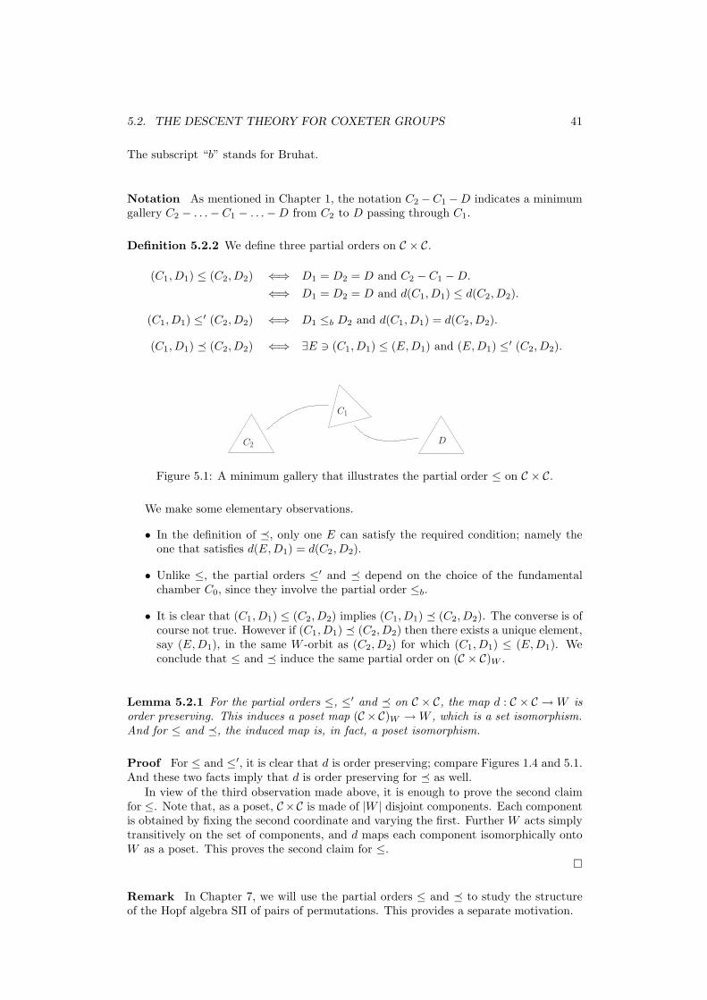
5.2. THE DESCENT THEORY FOR COXETER GROUPS 41
The subscript “b” stands for Bruhat.
Notation As mentioned in Chapter 1, the notation C2 −C1 −D indicates a minimumgallery C2 − . . .− C1 − . . .−D from C2 to D passing through C1.
Definition 5.2.2 We define three partial orders on C × C.
(C1, D1) ≤ (C2, D2) ⇐⇒ D1 = D2 = D and C2 − C1 −D.
⇐⇒ D1 = D2 = D and d(C1, D1) ≤ d(C2, D2).
(C1, D1) ≤′ (C2, D2) ⇐⇒ D1 ≤b D2 and d(C1, D1) = d(C2, D2).
(C1, D1) � (C2, D2) ⇐⇒ ∃E ∋ (C1, D1) ≤ (E,D1) and (E,D1) ≤′ (C2, D2).
C1
C2 D
Figure 5.1: A minimum gallery that illustrates the partial order ≤ on C × C.
We make some elementary observations.
• In the definition of �, only one E can satisfy the required condition; namely theone that satisfies d(E,D1) = d(C2, D2).
• Unlike ≤, the partial orders ≤′ and � depend on the choice of the fundamentalchamber C0, since they involve the partial order ≤b.
• It is clear that (C1, D1) ≤ (C2, D2) implies (C1, D1) � (C2, D2). The converse is ofcourse not true. However if (C1, D1) � (C2, D2) then there exists a unique element,say (E,D1), in the same W -orbit as (C2, D2) for which (C1, D1) ≤ (E,D1). Weconclude that ≤ and � induce the same partial order on (C × C)W .
Lemma 5.2.1 For the partial orders ≤, ≤′ and � on C × C, the map d : C × C →W isorder preserving. This induces a poset map (C ×C)W →W , which is a set isomorphism.And for ≤ and �, the induced map is, in fact, a poset isomorphism.
Proof For ≤ and ≤′, it is clear that d is order preserving; compare Figures 1.4 and 5.1.And these two facts imply that d is order preserving for � as well.
In view of the third observation made above, it is enough to prove the second claimfor ≤. Note that, as a poset, C ×C is made of |W | disjoint components. Each componentis obtained by fixing the second coordinate and varying the first. Further W acts simplytransitively on the set of components, and d maps each component isomorphically ontoW as a poset. This proves the second claim for ≤.
�
Remark In Chapter 7, we will use the partial orders ≤ and � to study the structureof the Hopf algebra SΠ of pairs of permutations. This provides a separate motivation.
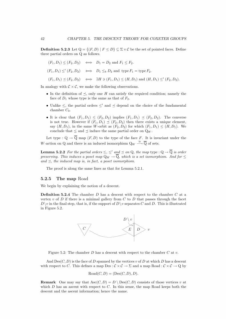
42 CHAPTER 5. THE DESCENT THEORY FOR COXETER GROUPS
Definition 5.2.3 Let Q = {(F,D) | F ≤ D} ⊆ Σ×C be the set of pointed faces. Definethree partial orders on Q as follows.
(F1, D1) ≤ (F2, D2) ⇐⇒ D1 = D2 and F1 ≤ F2.
(F1, D1) ≤′ (F2, D2) ⇐⇒ D1 ≤b D2 and typeF1 = typeF2.
(F1, D1) � (F2, D2) ⇐⇒ ∃H ∋ (F1, D1) ≤ (H,D1) and (H,D1) ≤′ (F2, D2).
In analogy with C × C, we make the following observations.
• In the definition of �, only one H can satisfy the required condition; namely theface of D1 whose type is the same as that of F2.
• Unlike ≤, the partial orders ≤′ and � depend on the choice of the fundamentalchamber C0.
• It is clear that (F1, D1) ≤ (F2, D2) implies (F1, D1) � (F2, D2). The converseis not true. However if (F1, D1) � (F2, D2) then there exists a unique element,say (H,D1), in the same W -orbit as (F2, D2) for which (F1, D1) ≤ (H,D1). Weconclude that ≤ and � induce the same partial order on QW .
Let type : Q → Q map (F,D) to the type of the face F . It is invariant under the
W -action on Q and there is an induced isomorphism QW
∼=−→ Q of sets.
Lemma 5.2.2 For the partial orders ≤, ≤′ and � on Q, the map type : Q→ Q is orderpreserving. This induces a poset map QW → Q, which is a set isomorphism. And for ≤and �, the induced map is, in fact, a poset isomorphism.
The proof is along the same lines as that for Lemma 5.2.1.
5.2.5 The map Road
We begin by explaining the notion of a descent.
Definition 5.2.4 The chamber D has a descent with respect to the chamber C at avertex v of D if there is a minimal gallery from C to D that passes through the facetD\v in the final step, that is, if the support ofD\v separates C and D. This is illustratedin Figure 5.2.
vC DE
D \ v
Figure 5.2: The chamber D has a descent with respect to the chamber C at v.
And Des(C,D) is the face ofD spanned by the vertices v ofD at whichD has a descentwith respect to C. This defines a map Des : C × C → Σ and a map Road : C × C → Q by
Road(C,D) = (Des(C,D), D).
Remark One may say that Asc(C,D) = D \ Des(C,D) consists of those vertices v atwhich D has an ascent with respect to C. In this sense, the map Road keeps both thedescent and the ascent information; hence the name.

5.2. THE DESCENT THEORY FOR COXETER GROUPS 43
Descent sets can be characterized in terms of the semigroup structure on Σ as follows.
Proposition 5.2.2 Given chambers C,D and a face F ≤ D, we have
FC = D ⇐⇒ Des(C,D) ≤ F.
Thus Des(C,D) is the smallest face F ≤ D such that FC = D.
The above observation is due to Brown [18, Proposition 4].
Lemma 5.2.3 For ≤ and �, the map Road : C × C → Q is order preserving.
Proof We prove the lemma only for the partial order ≤. Let (C1, D) ≤ (C2, D) andv ≤ Des(C1, D). To prove the lemma, we need to show that v ≤ Des(C2, D).
The first assumption gives a minimum gallery C2− . . .−C1− . . .−D and the second
gives a minimum gallery C1− . . .−ED\v
D. Replacing the second part of the first gallery
by the second gallery, one obtains a minimum gallery C2− . . .−C1− . . .−ED\v
D. Thisshows that v ≤ Des(C2, D).
�
5.2.6 The map GRoad
Next we introduce global descents. This notion is meaningful only when W is finite.Recall that in this case, there exists the notion of opposite faces. Let − : Σ → Σ be theopposite map that sends a face F to its opposite face F .
Definition 5.2.5 The chamber D has a global descent with respect to the chamber Cat the vertex v of D if, for every chamber E ∈ star(v), the star region of v, there is aminimal gallery from C to E that passes through the facet E \ v in the final step.
And GDes(C,D) is the face of D spanned by the vertices v of D at which D has aglobal descent with respect to C. This defines a map GDes : C × C → Σ and a mapGRoad : C × C → Q by
GRoad(C,D) = (GDes(C,D), D).
Note that by definition GDes(C,D) ≤ Des(C,D).
v
C
D
E C
Figure 5.3: The chamber D has a global descent with respect to the chamber C at v.
Proposition 5.2.3 We have GDes(C,D) = D ∩ C.
Proof Suppose that D has a global descent with respect to C at v, see Figure 5.3. Thedefinition implies that all chambers in star(v) have a descent (and global descent) withrespect to C at v. The fact mentioned after Equation (1.3) now implies that the oppositechamber C ∈ star(v).
Conversely, if C ∈ star(v) then the convexity of star(v) implies that all chambers instar(v) have a descent with respect to C at v.

44 CHAPTER 5. THE DESCENT THEORY FOR COXETER GROUPS
Lemma 5.2.4 For ≤ and �, the map GRoad : C × C → Q is order preserving.
Proof We only prove the lemma for the partial order ≤. Let (C1, D) ≤ (C2, D) andv ≤ GDes(C1, D) = D ∩ C1, that is, D,C1 ∈ star(v). To prove the lemma, we need toshow that C2 ∈ star(v).
v
C1
C2
D
C1
C2
D
v
The first assumption gives a minimum gallery C2 − . . . − C1 − . . . − D, which we canextend to D − . . .− C2 − . . .− C1 − . . .−D. Hence by restriction, we have a minimumgallery D− . . .−C2 − . . .−C1 such that D,C1 ∈ star(v). The convexity of a star regionnow implies that C2 ∈ star(v).
�
5.2.7 The map Θ
Next we introduce the map Θ. We continue to assume that W is finite. We first prove apreliminary fact.
Fact 5.2.1 Let F ≤ D and C be any chamber. Then
FD − C −D ⇐⇒ FC = D ⇐⇒ C ∈ reg(F,D).
The last equivalence is just the definition of reg(F,D), which is the lunar region of Fand D, as given in (2.6).
F F
H
C
DFD
Figure 5.4: A chamber C in the lunar region reg(F,D).
Proof The first equivalence is a consequence of the following three statements.
FC = D ⇐⇒If a hyperplane H separates C and D
then it does not pass through F .
H separates FD and D ⇐⇒ H does not pass through F.
FD − C −D ⇐⇒If a hyperplane H separates C and D
then it also separates FD and D.
Figure 5.4 shows the lunar region reg(F,D) and illustrates the situation in all the state-ments above. For the first two statements, one can argue with sign sequences using (1.1).The third statement is same as (1.3).
�

5.2. THE DESCENT THEORY FOR COXETER GROUPS 45
Definition 5.2.6 Let Θ : Q → C × C, where for F,D fixed, Θ(F,D) is the maximalelement of the poset {(C,D) | FC = D} in the partial order ≤ on C × C.
For Θ to be well-defined, we need to show that there is a unique maximum. Firstnote that FFD = FD = D. Hence (FD,D) ∈ {(C,D) | FC = D}. Now Fact 5.2.1implies that (FD,D) is the maximal element in {(C,D) | FC = D} in the partial order≤ on C × C. We have shown the following.
Proposition 5.2.4 We have Θ(F,D) = (FD,D).
C DF
CF
We also have (C,D) = Θ(F,D) ⇐⇒ (D,C) = Θ(F,C).
It follows from the gate property and the above proposition that:
Lemma 5.2.5 For ≤ and �, the map Θ : Q→ C × C is order preserving.
5.2.8 Connection among the three maps
Proposition 5.2.5 For ≤ and �, the maps Road and GRoad are the left and rightadjoints respectively to Θ. In other words,
(i) Road(C,D) ≤ (F,D) ⇐⇒ (C,D) ≤ Θ(F,D).
(ii) (F,D) ≤ GRoad(C,D) ⇐⇒ Θ(F,D) ≤ (C,D).
And the same statement with ≤ replaced by �.
Proof We prove the proposition only for the partial order ≤. Note that the result for� can be deduced using the result for ≤. To see (i), note that
Road(C,D) ≤ (F,D) ⇐⇒ FC = D ⇐⇒ (C,D) ≤ Θ(F,D). (5.5)
The first equivalence follows from Proposition 5.2.2 and the second from Fact 5.2.1 andProposition 5.2.4.
To see (ii), note that
(F,D) ≤ GRoad(C,D) ⇐⇒ F ≤ C ⇐⇒ F ≤ C
⇐⇒ D − C − FD −D ⇐⇒ C − FD −D
⇐⇒ Θ(F,D) ≤ (C,D).
The first equivalence is by Proposition 5.2.3. For the third equivalence, we use the gateproperty in one direction and the convexity of star(F ) and F ≤ D in the other direction.For the fourth equivalence, we use the fact mentioned after Equation (1.3). And for thelast equivalence, we use Proposition 5.2.4.
�
Proposition 5.2.6 The map Θ is a section to both Road and GRoad. In particular, itimplies that Θ is injective and Road and GRoad are surjective.

46 CHAPTER 5. THE DESCENT THEORY FOR COXETER GROUPS
Proof Let (C,D) = Θ(F,D). Then by Proposition 5.2.5,
Road(C,D) ≤ (F,D) ≤ GRoad(C,D).
However by definition, GRoad(C,D) ≤ Road(C,D). Hence
Road(Θ(F,D)) = (F,D) = GRoad(Θ(F,D)),
which proves the proposition.�
Remark It is clear that many results in this section hold for hyperplane arrangements.The objects W , Q, and L and the maps involving them, for example d and type, arespecial to the Coxeter case. The remaining part, with the exception of the partial orders≤′ and �, is valid for any central hyperplane arrangement.
Open Question It is not clear how to generalize the results in this section to LRBs.The problem starts right with defining the descent map. For that, one needs to assumethat a LRB satisfies the projection axiom (P2). These projection axioms were defined inMahajan [60, Chapter 1, page 15]. They are not to be confused with the axioms that wewill define in Chapter 6. Formulate the correct abstract framework to define descents,global descents and so forth.
5.3 The coinvariant descent theory for Coxeter groups
Let l : W → Z be the length function. In the previous section, we proved the existenceof the maps des, gdes : W → Q and θ : Q → W . In Sections 5.3.1-5.3.3, we explicitlydescribe these maps. As expected, they have very similar descriptions to the ones forthe maps Des,GDes and Θ. In Section 5.3.4, we deduce that the maps des and gdesare the left and right adjoints respectively to θ. In the rest of the section, we look atsome additional results. In Section 5.3.5, we discuss shuffles, and in Section 5.3.6, weconsider some sets that show up in the product in the M basis of the Hopf algebra ofpermutations SΛ. The later part will be relevant to Chapter 7.
Notation For T ≤ S and D ∈ C, it is convenient to write TD for the face of D of typeT .
5.3.1 The map des
Let C,D ∈ C be such that d(C,D) = w. Then by definition, des(w) is the type of theface Des(C,D). Let E ∈ C be such that d(D,E) = s. Hence from Equation (1.5), wehave d(C,E) = ws. Then in analogy with Definition 5.2.4, one can say:
The element w ∈W has a descent at s ∈ S if there is a minimum gallery C −E −D,or equivalently, if l(ws) < l(w). In other words:
Proposition 5.3.1 We have des(w) = {s ∈ S | l(ws) < l(w)}.
Thus, we recover the familiar notion of descent. Alternatively, from Proposition 5.2.2:
Proposition 5.3.2 Let C,D ∈ C and T ≤ S. Further let d(C,D) = w and TD be theface of D of type T . Then
TDC = D ⇐⇒ des(w) ≤ T.

5.3. THE COINVARIANT DESCENT THEORY FOR COXETER GROUPS 47
sC0 wC0wsC0
Figure 5.5: A descent at s for an element w ∈ W .
Since d(C0, wC0) = w, we can take for example C = C0 and D = wC0 and say thatdes(w) is the type of the face Des(C0, wC0). In analogy with Definition 5.2.4, one says:
The element w ∈W has a descent at s ∈ S if there is a minimum gallery from C0 towC0 passing through wsC0. This is illustrated in Figure 5.5.
Alternatively, from the above proposition, des(w) is the type of the smallest face Fsuch that FC0 = wC0.
Remark Following our earlier terminology, one should denote the map des by the term“road”. However in this particular case, such a distinction is not necessary because bytaking complement in the set S, the descent and ascent sets determine each other.
5.3.2 The map gdes
Let C,D ∈ C be such that d(C,D) = w. Then by definition, gdes(w) is the type of theface GDes(C,D). Since d(C0, wC0) = w, we can take C = C0 and D = wC0 and saythat gdes(w) is the type of the face GDes(C0, wC0). Applying Definition 5.2.5 gives usthe following.
Let v be the vertex of wC0 of type s. Then the element w ∈ W has a global descentat s ∈ S if s ∈ des(u) for every uC0 ∈ star(v).
s
C0
C0
uC0 wC0
Figure 5.6: A global descent at s for an element w ∈W .
The chambers in star(v) are characterized by the set {wzC0 | z is any word writtenusing generators other than s}. Hence w ∈ W has a global descent at s ∈ S if l(wzs) <l(wz), for any word z written using generators other than s.
Proposition 5.3.3 We have gdes(w) = {s ∈ S | l(wzs) < l(wz) for any word z writtenusing generators other than s}.
5.3.3 The map θ
Let θ : Q→W be the map induced from Θ : Q→ C×C. The analogy with Definition 5.2.6is given later in Proposition 5.3.7. In analogy with Proposition 5.3.4, one can say:
Proposition 5.3.4 For T ∈ Q, let TD be the face of type T of D. Then θ : Q → W isgiven by T 7→ θ(T ) where θ(T ) = d(TDD,D).

48 CHAPTER 5. THE DESCENT THEORY FOR COXETER GROUPS
Corollary 5.3.1 For T ∈ Q, let TC0be the face of type T of C0. Then θ : Q → W is
given by T 7→ θ(T ) where
θ(T ) = d(C0, TC0C0), or equivalently, θ(T )C0 = TC0
C0.
C0 TC0
C0
TC0
C0TC0
Proof Take D = TC0C0 in the previous proposition. The face TD of type T of D is
TC0. Hence TC0
D = TC0TC0
C0 = TC0C0 = C0.
�
Remark It may not be true that TC0= TC0
, where TC0is the face of type T of C0.
This is because the opposite map does not preserve types in general.
C0C0
Figure 5.7: The image of the θ map in rank 3.
The corollary says that except for C0, the image of the map θ viewed as distancefrom C0, is concentrated around C0. Alternatively, it isolates a set of “long” elements ofW . Consider the rank 3 case when W has 3 generators. The image of the θ map thenconsists of 23 = 8 chambers. A schematic picture for that is shown in Figure 5.7.
5.3.4 Connection among the three maps
The map d : C × C → W has a section given by w 7→ (w−1C0, C0). Similarly, the maptype : Q → Q has a section given by T 7→ (TC0
, C0), where TC0is the face of type T of
C0. Further, both the sections are order preserving for each of the partial orders ≤ and�.
Note that the second coordinate in the image of both maps is always C0. Further,the maps Road, GRoad and Θ preserve the second coordinate. Since the action of Wis simply transitive on C, and W and Q are the orbit spaces of C × C and Q respectively,we obtain three commutative diagrams.
C × C
Road����
W?_oo
des����
Q Q?_oo
C × C
GRoad����
W?_oo
gdes����
Q Q?_oo
C × C W?_oo
Q
Θ
OO
Q?_oo
θ
OO
(5.6)
Using diagrams (5.3) and (5.6), now Propositions 5.2.5 and 5.2.6 yield the followingcorollaries respectively.

5.3. THE COINVARIANT DESCENT THEORY FOR COXETER GROUPS 49
Proposition 5.3.5 The maps des and gdes are the left and right adjoints respectively toθ. In other words,
(i) des(w) ≤ T ⇐⇒ w ≤ θ(T ).
(ii) T ≤ gdes(w) ⇐⇒ θ(T ) ≤ w.
Proposition 5.3.6 The map θ is a section to both des and gdes.
5.3.5 Shuffles
This subsection is optional. By using the map des, we define the notion of shuffles for aCoxeter group. We then describe it by more geometric objects and explain how the mapθ fits into the picture. The motivation for the terminology comes from the example oftype An−1 given in Section 5.4.6.
Definition 5.3.1 For T ≤ S, define the set of T -shuffles by
ShT = {σ ∈W | des σ ≤ T }.
Let ΣT be the set of faces in Σ of type T . For a fixed T ≤ S, one can write
C =⊔
F∈ΣT
CF , where CF = {D | F ≤ D}.
This is because every chamber D ∈ C has a unique face of type T .Recall that we have fixed a fundamental chamber C0 in C. In each star region CF ,
by the gate property, there is a special chamber, namely FC0, closest to C0 in thegallery metric. Under the identification of C with W , it corresponds to a T -shuffle. Moreprecisely:
Lemma 5.3.1 There is a bijection
π : ΣT → ShT
given by F 7→ σ, where FC0 = σC0, or equivalently, σ = d(C0, FC0). Under thisbijection, TC0
, the face of type T of C0 maps to θ(T ).
In the identity FC0 = σC0, the left hand side is the product of F and C0 while the righthand side is the action of σ on C0.
Proof The first fact is a simple consequence of Proposition 5.3.2. The second factfollows from Corollary 5.3.1.
�
Figure 5.8 shows two bold dots, which are faces of type T , along with their starregions. The element σ = d(C0, FC0), which corresponds to F , has been shown as avector pointing from C0 to FC0.
Lemma 5.3.2 Let T ≤ S and D ∈ C be fixed, and let TD be the face of D of type T .Then the distance map
d : {(C,D) | C ∈ reg(TD, D)} −→ ShT
is a bijection. Under this bijection, (TDD,D) maps to θ(T ). And further
ShT = {σ ∈W | σ−1C0 ∈ reg(TC0, C0)}.

50 CHAPTER 5. THE DESCENT THEORY FOR COXETER GROUPS
C0
σ
θ(T )
C0
FFC0
TC0
TC0
C0
Figure 5.8: T -shuffles correspond to faces of type T .
Note that, in the left hand side in the above bijection, the second coordinate is alwaysfixed to be D. This bijection is dual to the one in Lemma 5.3.1, where the first coordinateis fixed to be C0. For more on this duality, see Mahajan [60, Chapter 1, pages 32-36].
Proof Observe that by definition,
C ∈ reg(TD, D) ⇐⇒ TDC = D.
The first claim now follows from Proposition 5.3.2. The second claim follows from Propo-sition 5.3.4. Setting D = C0 yields the third claim.
�
Remark Note that by the above lemma, the set
{σ ∈ W | des(σ−1) ≤ T },
closely related to ShT , corresponds to chambers in the lunar region of TC0and C0. This
makes the connection between shuffles and lunar regions precise. The reader may lookat the definition of the product in SΛ in this regard (Definition 7.2.13).
Proposition 5.3.7 The element θ(T ) is the maximal element in ShT in the weak leftBruhat order on W . Equivalently,
FC0 ≤b TC0C0
for any face F of type T .
Proof We know from Definition 5.2.6 and Proposition 5.2.4 that (TDD,D) is the max-imal element in {(C,D) | C ∈ reg(TD, D)}. Hence the result follows from Lemma 5.3.2and the fact that d is order preserving.
�
For W = Sn, the above result is written in [4, Lemma 2.8]. In Chapter 7, we willgeneralize this result further. For that purpose, the following direct proof of the aboveproposition will be useful.
Alternative proof Let FC0 = uC0 and TC0C0 = vC0. We want to show that there is
a minimum gallery C0− vu−1C0− vC0. For that, observe that vu−1 takes FC0 to TC0C0
and hence F to TC0. Therefore
TC0(vu−1C0) = vu−1(FC0) = TC0
C0.

5.3. THE COINVARIANT DESCENT THEORY FOR COXETER GROUPS 51
This says that TC0C0 is the gate of star(TC0
) when viewed from vu−1C0. Hence by thegate property, we have,
C0 − vu−1C0 − TC0
C0 − C0.
By restriction, we obtain the required minimum gallery.2
5.3.6 Sets related to the product in the M basis of SΛ
This subsection is optional for this chapter. Let T ≤ S and WS\T be the parabolicsubgroup of W generated by S \ T . Let w ∈ W and x ∈ WS\T . Further let G ≤ C0 bethe face of type T of the fundamental chamber.
Lemma 5.3.3 The sets S0w(x), S+
w (x) and S−w (x), defined below, are in bijection with
one another.
The definition of the set S0w(x) has a geometric flavor, while definitions of the other
two sets have a combinatorial flavor. These sets show up when one considers the productin the M basis of the Hopf algebra of permutations SΛ. We will see this in Chapter 7.Though this motivation is specific to type An−1, the discussion below is general. Wesuppress the dependence on T in the notation.
Definition 5.3.2
S0w(x) =
(C,D) ∈ C × C, d(C,D) = w,GD = C0
∣∣∣∣(i) C −GC −GD −D
(ii) GC = x−1C0.
Note that this definition depends on the choice of C0. From the gate property, there aretwo shorter ways to rewrite condition (i), namely, C −GC −D, or C −GD −D.
C
x−1C0 C0
D
G
GG
Figure 5.9: The set S0w(x).
To get a general idea of what is going on, the reader may refer to Figure 5.9. In thefigure, the face G is shown as a vertex. The two lunar regions, containing the chambersC and D respectively, lie on a sphere and meet at G, the vertex opposite to G. Forsimplicity, this is not shown in the figure, where there are two vertices labeled G.
We have defined S0w(x) using the Coxeter complex Σ. Since d(C,D) = w, knowing D
determines C and vice versa. So one can also define S0w(x) using the Coxeter group W
by getting rid of one of the coordinates. This leads to two more sets S+w (x) and S−
w (x)as below.
Let d(D,C0) = σ. Then by Proposition 5.3.2,
σ ∈ ShT ⇐⇒ GD = C0.
So S0w(x) can be rewritten as
σ ∈ ShT
∣∣∣∣(i) C −GC −GD −D
(ii) GC = x−1C0.
,

52 CHAPTER 5. THE DESCENT THEORY FOR COXETER GROUPS
where D and C are defined by d(D,C0) = σ and d(C,D) = w.
Note that a gallery condition can be rephrased using the partial order ≤ on C × C.And using the order preserving map d, one can then write it using the weak left orderon W . Hence condition (i) can be rewritten in two ways as follows.
d(GC,D) ≤ d(C,D) ⇐⇒ xσ−1 ≤ w, or d(GD,D) ≤ d(C,D) ⇐⇒ σ−1 ≤ w.
Further note that, if xσ−1 ≤ w then
GC = x−1C0 ⇐⇒For E ∈ star(G), a minimum gallery C − E −D implies
a minimum gallery x−1C0 − E − C0.
This follows from the gate property. Now let d(E,C0) = y ∈ WS\T , that is, E = y−1C0.Note that y and E determine each other. Now the right hand side in the above equationcan be rewritten as:
For x, y ∈WS\T , if yσ−1 ≤ w, then y ≤ x.
This motivates the following definition.
Definition 5.3.3
S+w (x) =
σ ∈ ShT
∣∣∣∣(i) xσ−1 ≤ w.
(ii) For y ∈WS\T , if yσ−1 ≤ w, then y ≤ x.
For type An−1, the above set is considered in [4, Equations (4.2) and (4.4)].
Analogous to the analysis above, instead of d(D,C0) = σ, we can start with theequation d(C, x−1C0) = σ. Then by Proposition 5.3.2,
σ ∈ ShT ⇐⇒ GC = x−1C0.
This leads us to the following.
Definition 5.3.4
S−w (x) =
σ ∈ ShT
∣∣∣∣(i) x−1σ−1 ≤ w−1.
(ii) For y ∈WS\T , if y−1σ−1 ≤ w−1, then y−1 ≤ x−1.
In the above discussion, along with the definitions, we also indicated the proof of Lemma 5.3.3.The details can be filled in by the reader.
5.4 The example of type An−1
This example arises from W = Sn, the symmetric group on n letters (Section 1.4). Wenow explain this example in direct combinatorial terms without reference to hyperplanearrangements or the general theory of Coxeter groups. We use the superscript n toindicate the dependence on n.

5.4. THE EXAMPLE OF TYPE AN−1 53
5.4.1 The posets Σn and Ln
We quickly recall the content of Section 1.4.3. The Coxeter complex Σn can be identifiedwith the poset of compositions F = F 1| . . . |F l of the set [n]. For example, 347|16|258 isan element of Σ8. We multiply two set compositions by taking intersections and orderingthem lexicographically; more precisely, if F = F 1| . . . |F l and H = H1| . . . |Hm, then
FH = (F 1 ∩H1| . . . |F 1 ∩Hm| . . . |F l ∩H1| . . . |F l ∩Hm) ,
where the hat means “delete empty intersections”. For example,
(347|16|258)(6|157|28|34) = (7|34|6|1|5|28).
For the partial order of Σn, we say F ≤ K if K is a refinement of F . The set ofchambers Cn in Σn consists of set compositions with singleton blocks, so they correspondto permutations of [n]. The opposite F of a face F = F 1| . . . |F l is obtained by reversingthe order of the blocks, that is, F = F l| . . . |F 1.
The lattice Ln is the poset of set partitions again under refinement and the supportmap supp : Σn ։ Ln forgets the ordering of the blocks. For example,
supp(347|16|258) = {347, 16, 25}.
5.4.2 The posets Qn and Zn
By definition, Qn consists of pairs (F,D), where F is a set composition and D is a setcomposition with singleton blocks that refines F . For example,
(236|15|4, 6|2|3|5|1|4) ∈ Q6.
It is convenient to write this element as (6|2|3|5|1|4), using small and big bars. We callthis a fully nested set composition of [6]. Similarly, the poset Zn associated to Qn canbe described using fully nested set partitions.
Table 5.1: Combinatorial notions for type An−1.
Σn = set compositions Qn = fully nested set compositions
Ln = set partitions Zn = fully nested set partitions
Definition 5.4.1 A nested set composition is a sequence F = F 1|F 2| . . . |F l, in which
each F i is a set composition of Ai, and A1| . . . |Al is a set composition of [n]. For example,
(3|15|7|48|29|6)
is a nested composition of [9]. A fully nested set composition is a nested set compositionwith singleton blocks.
Equivalently, a nested set composition is a pair (F,H) of set compositions such thatF ≤ H . In the above example, the pair is (135|24789|6, 3|15|7|48|29|6). And a fullynested set composition is a pair (F,D) with F ≤ D and D a chamber.
Definition 5.4.2 A nested set partition is a set L = {L1, . . . , Ll}, in which each Li is aset composition of Ai, and {A1, . . . , Al} is a set partition of [n]. For example,
{3|56, 2|17, 4}
is a nested partition of [7]. A fully nested set partition is a nested set partition withsingleton blocks.

54 CHAPTER 5. THE DESCENT THEORY FOR COXETER GROUPS
We now describe the partial orders on Qn and Zn in this language. We say x ≤ y
in Qn if y is obtained from x by replacing zero or more occurrences of a small bar by abig bar. Similarly, we say x ≤ y in Zn if y is obtained from x by deleting zero or moreoccurrences of a bar. For example,
(3|1|5|4|2|6) ≤ (3|1|5|4|2|6) in Q6 {3|5, 2|1, 4} ≤ {3, 5, 2|1, 4} in Z5.
Next we describe the maps related to these two objects. The map Qn → Σn forgets thesmall bars, and replaces the big bars by small bars. For example,
(6|2|3|5|1|4) 7→ (236|15|4).
The map lune : Qn → Zn forgets the big bars. For example,
lune(6|2|3|5|1|4) = {6|2|3, 5|1, 4}.
The map Zn → Ln forgets the small bars. For example,
{6|2|3, 5|1, 4} 7→ {236, 15, 4}.
As already mentioned, the map supp : Σn → Ln forgets the ordering among the blocks,or equivalently, forgets the small bars.
5.4.3 The quotient posets Qn
and Ln
The symmetric group Sn acts on Σn and Qn. The set of Sn-orbits in both cases can beidentified with the set of compositions of n, which we denote Q
n. The induced partial
order on Qn
is given by refinement of compositions. The quotient map type : Σn → Qn
(resp. Qn → Qn) sends a set composition (resp. fully nested set composition) to its
underlying composition. For example,
type(347|16|258) = (3, 2, 3).
The symmetric group Sn acts on Ln and Zn. The set of Sn-orbits in both cases can beidentified with the set of partitions of n, which we denote L
n. The induced partial order
on Ln
is as given in Definition 3.2.1. The map Ln → Ln
(resp. Zn → Ln) sends a set
partition (resp. fully nested set partition) to its underlying partition. For example,
{347, 16, 258} 7→ (3, 3, 2).
The maps supp : Σn → Ln and lune : Qn → Zn induce the map Qn→ L
nwhich sends a
composition to its underlying partition.
Remark We have explained combinatorially all the objects and maps that occur indiagram (5.4) for this particular example.
5.4.4 The maps Road, GRoad and Θ
The projection and opposite map for type An−1 were explicitly described in Section 5.4.1.The maps Des,GDes and Θ can be written by applying Propositions 5.2.2, 5.2.3 and 5.3.4to these descriptions.
Definition 5.4.3 The descent map Des : Cn × Cn → Σn is defined as follows.
• Des(C,D) = F is the face of D = D1|D2| . . . |Dn such that Di and Di+1 lie indifferent blocks of F iff Di appears after Di+1 in C.

5.4. THE EXAMPLE OF TYPE AN−1 55
For example, Des(2|4|1|3, 1|4|3|2) = (1|34|2).
Definition 5.4.4 The global descent map GDes : Cn × Cn → Σn is defined as follows.
• GDes(C,D) = F is the face of D = D1|D2| . . . |Dn such that Di and Di+1 lie indifferent blocks of F iff Dj appears after Dk in C for all j ≤ i and i+ 1 ≤ k.
For example, GDes(2|4|1|3, 1|4|3|2) = (134|2).
Definition 5.4.5 The map Θ : Qn → Cn × Cn is defined as follows.
• Θ(F,D) = (C,D), where C is obtained by reversing the order on the blocks of Fand ordering the elements within each block using the order of D.
For example, Θ(2|5|1|6|3|7|4) = (4|6|3|7|1|2|5, 2|5|1|6|3|7|4).
5.4.5 The maps des, gdes and θ
The maps Des,GDes : Cn ×Cn → Σn and Θ : Qn → Cn × Cn are maps of Sn-sets. Hencethey induce maps des, gdes : Sn → Q
nand θ : Q
n→ Sn on the Sn-orbits. The map des
gives the usual notion of descent of a permutation and the maps gdes and θ coincide withthe definitions given in [4]. We now describe them.
Write a permutation w ∈ Sn using the one-line notation as w1w2 . . . wn. Recall thatthe generating set S is {s1, . . . , sn−1}, where si is the transposition (i, i+ 1). Note thatsiw interchanges the letters i and i+ 1, while wsi interchanges the letters in positions iand i+ 1. In other words, wsi = w1w2 . . . wi+1wi . . . wn. Note that
l(wsi) < l(w) ⇐⇒ wi > wi+1.
Hence by Proposition 5.3.1, one obtains:
Definition 5.4.6 The element w has a descent at si (or position i) if wi > wi+1.
Now we explain the map gdes. Observe that the set
{z | z can be written using generators other than si}
consists of precisely those permutations which can be written as a permutation of thefirst i letters followed by a permutation of the remaining n − i letters. For such a z,we have wz = w1 . . . wi︸ ︷︷ ︸
permuted
wi+1 . . . wn︸ ︷︷ ︸permuted
. Combining with the above definition of des and the
definition of gdes given by Proposition 5.3.3, one obtains:
Definition 5.4.7 The element w has a global descent at si (or position i) if wj > wk
for all j ≤ i and k ≥ i+ 1.
Now we explain the map θ. The fundamental chamber C0 is the set composition(1|2| . . . |n) and its opposite chamber C0 is (n|n − 1| . . . |2|1). Let T = {t1 < · · · < tk}be any subset of [n − 1]. The face of type T of C0 is then given by the k block setcomposition
(n−t1+1 . . . n| n−t2+1 . . . n−t1| . . . |1 . . . n−tk).
Multiplying on the right by C0 and using Proposition 5.3.4, we obtain:
Definition 5.4.8 For T ≤ S, we have
θ(T ) = (n−t1+1| . . . |n| n−t2+1| . . . |n−t1| . . . |1| . . . |n−tk).

56 CHAPTER 5. THE DESCENT THEORY FOR COXETER GROUPS
5.4.6 Shuffles
Let T = {t1 < · · · < tk} be any subset of [n− 1]. It follows from the definitions that
ShT = {σ ∈ Sn | σ1 < σ2 < · · · < σt1 , σt1+1 < · · · < σt2 , . . . , σtk−1+1 < · · · < σtk}.
As an example, let n = 4 and T = {2}. Then in the composition notation, T = (2, 2)and
ShT = {1|2|3|4, 1|3|2|4, 1|4|2|3, 2|3|1|4, 2|4|1|3, 3|4|1|2}.
The set of inverses of the six elements obtained by shuffling 1|2 and 3|4 is precisely theset above. This explains the shuffle terminology used in Section 5.3.5.
5.5 The toy example of type A×(n−1)1
In this section, we give a toy example to illustrate the theory. It deals with the coordinatehyperplane arrangement arising from the Coxeter group Z
n−12 , that is, the Coxeter group
of type A×(n−1)1 . One reason we stress this example is that it belongs to an infinite
family and hence is relevant to external structures. As in the previous example, we usethe superscript n to indicate the dependence on n.
First note that Z2 or equivalently S2 is the Coxeter group of type A1 generated by asingle element of order 2. By taking direct product of n− 1 copies of Z2, we obtain theCoxeter group Z
n−12 with generating set S = {s1, . . . , sn−1} and presentation as below.
s2i = 1, (sisj)2 = 1 if i 6= j.
The reflection arrangement in this case is the coordinate arrangement in Rn−1. It consists
of the hyperplanes defined by xi = 0, where 1 ≤ i ≤ n − 1. The generator si acts onthe arrangement by changing the ith coordinate to its negative and keeping the othercoordinates unchanged.
We now explain the relevant objects for this example in direct combinatorial termswithout reference to hyperplane arrangements.
5.5.1 The posets Σn and Ln
Let Σn be the poset
+
////
/ −
�����
0
×+
////
/ −
�����
0
× · · · ×+
////
/ −
�����
0︸ ︷︷ ︸n−1
Namely, elements of Σn are sequences F = F 1F 2 . . . Fn−1 of length n−1 in the alphabet{+, 0,−}. And F ≤ K in Σn if K is obtained by replacing some of the zeroes in F byeither a + or a −. The product FK is the face with sign sequence
(FK)i =
F i if F i 6= 0,
Ki if F i = 0.(5.7)
This is the usual product rule in an oriented matroid as written in (1.1). Chambers inΣn are sequences of length n− 1 in the alphabet {+,−}. The opposite F of a face F isobtained by changing a + to a − and viceversa.
The lattice Ln can be identified with subsets of [n− 1], that is, Qn, but under reverse
inclusion. The map supp : Σn → Ln indicates the positions of the zero elements of a signsequence.

5.5. THE TOY EXAMPLE OF TYPE A×(N−1)1 57
5.5.2 The posets Qn and Zn
The elements of Qn can be regarded as stacked signed sequences. For example,
(+0 −
−0 +−
+0
)∈ Qn
and stands for the pair (0− 0 + −0,+−− + −+). For the partial order on Qn, we saythat x ≤ y if y is obtained from x by replacing zero or more occurrences of a stack bythe sign on top of the stack. For example,
(+0 −
−0 +−
+0
)≤
(+0 −−+−
+0
).
The elements of Zn are signed subsets of [n−1]. For example, {+1,−3,+6} is an elementof Z7. The partial order on Zn is reverse inclusion. For example,
{+1,−3,+6} ≤ {+1,+6}.
The map Qn → Σn forgets the signs above the zeroes. For example,
(+0 −
−0 +−
+0
)7→ 0− 0 +−0.
The map lune : Qn → Zn picks the positions of the zero elements and assigns them thesigns on top. For example,
(+0 −
−0 +−
+0
)7→ {+1,−3,+6}.
The map Zn → Ln = Qn
just forgets the signs of the signed set.
5.5.3 The quotient posets Qn
and Ln
The group Z2 acts on {+,−} where the nontrivial element of Z2 flips signs. This inducesan action of the group Z
n−12 on Σn and Qn. The set of orbits in both cases can be
identified with the set of compositions of n, which we denote Qn. The induced partial
order on Qn
is given by refinement of compositions. The quotient map type : Σn → Qn
indicates the positions of the nonzero elements of the sign sequence. The quotient maptype : Qn → Q
nindicates the positions of the nonzero elements of the stacked sign
sequence. For example,
type
(+0 −
−0 +−
+0
)= {2, 4, 5}.
Similarly the group Zn−12 acts on Zn and Ln. The set of orbits denoted L
nis the same
in both cases. Every element of Ln is fixed by Zn−12 . Hence the set of orbits L
n ∼= Ln.
The quotient map Zn → Ln
just forgets the signs of the signed set.The maps supp : Σn → Ln and lune : Qn → Zn induce the map Q
n→ L
nwhich is
an isomorphism sending a subset to its complement.
Remark We have explained combinatorially all the objects and maps that occur indiagram (5.4) for this particular example.
Remark The distance map d : Cn × Cn → Zn−12 sends (C,D) to the product of those
si’s for which Ci 6= Di. The order of the si’s is not important since Zn−12 is abelian. In
fact, the family Zn2 , as n varies, are the only abelian Coxeter groups.

58 CHAPTER 5. THE DESCENT THEORY FOR COXETER GROUPS
5.5.4 The maps Des, GDes and Θ
Definition 5.5.1 The notion of descent and global descent coincides for this example.We have
Des(C,D) = GDes(C,D) = F, where F i =
{0 if Ci = Di,
Di otherwise.
For example, Des(+−−+,−+−+) = −+ 00.
Definition 5.5.2 For the map Θ, we have
Θ(F,D) = (C,D), where
{Ci = Di if F i = 0,
Ci 6= Di if F i 6= 0.
For example, Θ(+00−,+ +−−) = (−+−+,+ +−−).
5.5.5 The maps des, gdes and θ
Note that as a set, Zn−12 can be indentified with the set of words of length n− 1 in the
alphabet {0, 1}. For example, for n = 6,
s2s4 ←→ (0, 1, 0, 1, 0).
Passing to orbits, we obtain the map des, gdes : Zn−12
∼=−→ Qn
that sends a word to thesubset that indicates the positions of the 1’s. It is an isomorphism in this case. The
induced map θ : Qn ∼=−→ Z
n−12 is the inverse to the above map.
5.6 The commutative diagram (5.8)
The goal of this section is to prove the following theorem.
Theorem 5.6.1 For Σ a left regular band (LRB), the following diagram of vector spacescommutes.
KΣb∗ //
supp
����Υ∗
��888
8888
8888
8888
8888
888 KQ
Θ //
lune
����Ψ
%%KKKKKKKKKKKKKKKKKKKKKKKKKKKKKKKKK K(C × C)
s
&&MMMMMMMMMM
K(C × C)∗
Road
��
KLb∗ //
Φ
""FFFFFFFFFFFFFFF KZ
Υ
))SSSSSSSSSSSSSSSSSSSSSSSSSSSSSS
KZ∗ � � lune∗ //
b��
KQ∗
b��KL∗ � �
supp∗//KΣ∗
(5.8)
For simplicity, we have abbreviated the base map to the letter b. If Σ is the Coxetercomplex of a Coxeter group W then the above is a commutative diagram of W -modules.
Note on the proof The proof is given in two parts. Cutting along the map Ψ, theabove diagram splits into two halves. The commutativity of each half is proved separately(Propositions 5.6.1 and 5.6.7). The organization is as below.
Let Σ be a Coxeter complex. Recall from Sections 5.2.3 and 5.2.4 that given Σ, onecan construct posets L,Q,Z and C × C. As remarked at the end of Section 5.2, apart

5.6. THE COMMUTATIVE DIAGRAM (5.8) 59
from the absence of the partial orders ≤′ and �, everything works the same for theposet of faces of any central hyperplane arrangement. In Section 5.6.1, we explain howthe ten objects in diagram (5.8) are constructed from these posets. In Sections 5.6.2and 5.6.3, we define the maps s, Θ, Road and Ψ and in Section 5.6.4 show that they fitin a commutative diagram (Proposition 5.6.1). The maps Θ and Road are defined usingthe corresponding maps in Section 5.2. We then explain how to adapt the proof to thecase when Σ is a LRB, or a projection poset. This is the top half of diagram (5.8).
For the bottom half of diagram (5.8), we directly work with a LRB. We use the resultsfrom Sections 2.2 and 2.5, where most of the work is done. The strategy is to break thediagram into five smaller diagrams as below. In Section 5.6.5, we define the maps supp,lune and base∗ and show that they fit in a commutative diagram. In Section 5.6.6, wedualize to get four more maps and the dual commutative diagram. In Section 5.6.7, weexplain the maps Φ and Υ. In Section 5.6.8, we draw three more commutative diagrams,which then imply the result (Proposition 5.6.7).
2
Remark Observe that scaling the five maps, namely, s,Ψ,Φ,Υ and Υ∗ by the samefactor does not affect the commutativity of the diagram.
5.6.1 The objects in diagram (5.8)
Let Σ be a Coxeter complex. The ten objects we consider are the vector spaces KΣ, KL,KQ, KZ, K(C × C) over K and their duals. The superscript ∗ refers to the dual space orthe dual map. Since each space is constructed by linearizing a poset, it has a canonicalbasis. However, in certain cases, it is better to use the partial order to define more bases,see Table 5.2.
Table 5.2: Vector spaces associated to Σ and their bases.
Vector space Bases Dual space Dual bases
KΣ H KΣ∗ M
KQ R,H,K KQ∗ S,M,F
K(C × C) R,H,K K(C × C)∗ S,M,F
KL h, q KL∗ m, p
KZ h KZ∗ m
For example, for both KQ and K(C × C), we let K be the canonical basis. We thendefine the R and H bases by the first two formulas below.
HA =∑
B≤A
KB, RA =∑
B�A
KB, RA =∑
B≤′A
HB , (5.9)
where A and B are elements of the underlying poset, and ≤, � and ≤′ are the partialorders given in Definitions 5.2.2 and 5.2.3. The last equality above follows from definitionsof the partial orders. For example,
H(E,C) =∑
(D,C)≤(E,C)
K(D,C) in K(C × C) and H(P,C) =∑
Q≤P
K(Q,C) in KQ,

60 CHAPTER 5. THE DESCENT THEORY FOR COXETER GROUPS
and so on. The M (resp. F ) basis is defined as dual to the H (resp. K) basis. It followsfrom (5.9) that
FB =∑
B≤A
MA, FB =∑
B�A
SA, MB =∑
B≤′A
SA. (5.10)
The case of KL is a little different. Instead of the H and K bases, we have the h andq bases related by
hX =∑
X≤Y
qY in KL. (5.11)
Dually, KL∗ has the m and p bases related by
pY =∑
X≤Y
mX in KL∗. (5.12)
The motivation for the q and p bases comes from the algebra structure of KL, seeLemma 5.6.3.
Remark The R and S bases are specific to the Coxeter case, since they involve thepartial orders ≤′ and �. Apart from that, the above discussion and what follows worksfor the poset of faces of any central hyperplane arrangement.
Example Recall from Section 5.4 that for the symmetric group Sn, the poset L, whichwe denoted Ln, is indexed by partitions of the set [n]. In this case, the graded vectorspace
ΠL∗ = ⊕n≥0
K(Ln)∗
is called the space of symmetric functions in noncommuting variables. It has a theorysimilar to that of symmetric functions. The definitions of the p and m bases abovecoincide with those considered by Gebhard, Rosas and Sagan [33, 83]; namely, p andm are the power and monomial basis respectively. The map Φ is an isomorphism inthis case. If we push the h basis from KL to KL∗ using Φ then it gives a basis of ΠL∗ ,denoted by the same letter in [83]. The map Φ is induced by a bilinear form on KL, seeDefinition 5.6.4. Pushing this form to KL∗ via Φ gives an inner product on ΠL∗ , withthe h and m bases being dual. The p basis is a lift of the power sum basis of symmetricfunctions. For more explanation, see Section 5.7.1 and Definition 5.7.8.
Remark The spaces Π (short for ΠL∗) and NΛ provide different noncommutative ana-logues to Λ, the space of symmetric functions (Section 3.2). Our treatment brings clarityto this distinction.
5.6.2 The maps s, Θ and Road
Definition 5.6.1 We define the switch map s : K(C × C)→ K(C × C)∗ by
K(D,C) 7→ F(C,D).
Lemma 5.6.1 Let Θ : Q→ C × C be the map defined in Section 5.2. The following arethree equivalent definitions of the map Θ : KQ→ K(C × C).
Θ(K(P,C)) =∑
Des(D,C)=P
K(D,C) (K basis).
Θ(H(P,C)) = HΘ(P,C) (H basis).
Θ(R(P,C)) = RΘ(P,C) (R basis).

5.6. THE COMMUTATIVE DIAGRAM (5.8) 61
Proof The equivalence of the first two definitions can be seen by a simple computation.We use the formula in the K basis to derive the formula in the H basis.
Θ(H(P,C)) =∑
(Q,C)≤(P,C)
Θ(K(Q,C)) =∑
Road(D,C)≤(P,C)
K(D,C)
=∑
(D,C)≤Θ(P,C)
K(D,C) = HΘ(P,C).
For the third equality, we used Proposition 5.2.5, part (i). The first and last equalitiesfollow from (5.9), which is the relation between the H and K bases.
Replacing H by R and ≤ by � in the computation, and using Proposition 5.2.5, part(i), one gets the equivalence between the first and third definitions.
�
The map Road : K(C × C)∗ → KQ∗ is defined as the dual to the map Θ : KQ →K(C × C). By duality, Lemma 5.6.1 gives:
Lemma 5.6.2 The following are three equivalent definitions of the map Road : K(C ×C)∗ → KQ∗.
Road(F(C,D)) = FRoad(C,D) (F basis).
Road(M(C,D)) =
MRoad (C,D) if (C,D) = Θ(Road(C,D))
0 otherwise.(M basis).
By replacing M by S, one gets the expression on the S basis.
A particularly useful expression for the map Θ is obtained when we start in the Hbasis and end in the K basis. It is given by the equation
Θ(H(P,C)) =∑
D: PD=C
K(D,C). (5.13)
This can be seen by using the first part of the computation in Lemma 5.6.1 and Equa-tion (5.5). Similarly, an useful expression for Road is obtained by going from the F basisto the M basis. It is given by
Road(F(C,D)) =∑
F : FC=D
M(F,D). (5.14)
An important feature of the above two formulas is that they are defined solely in termsof projection maps, and thus make sense not only for hyperplane arrangements or LRBs,but also for projection posets. We will exploit this feature in Chapter 6.
5.6.3 The bilinear form on KQ
Define a symmetric bilinear form on KQ by
〈H(P,C), H(F,D)〉 =
1 if FC = D and PD = C,
0 otherwise.
The above bilinear form induces a map Ψ : KQ 7→ KQ∗ given by
Ψ(H(P,C)) =∑
(F,D)
〈(P,C), (F,D)〉 M(F,D). (5.15)
A detailed discussion on this bilinear form is given in Section 2.5.

62 CHAPTER 5. THE DESCENT THEORY FOR COXETER GROUPS
5.6.4 The top half of diagram (5.8)
Proposition 5.6.1 For Σ a LRB, or more generally, a projection poset, the top half ofdiagram (5.8) commutes.
KQΘ //
Ψ
��
K(C × C)
s
��KQ∗
K(C × C)∗Road
oo
Proof First, let Σ be a central hyperplane arrangement. We want to show that Ψ =Road ◦s ◦ Θ. This is a direct computation. From Equation (5.13) and Definition 5.6.1,we obtain
s ◦Θ(H(P,C)) =∑
D: PD=C
F(C,D).
Now by Equation (5.14),
Road ◦s ◦Θ(H(P,C)) =∑
D: PD=C
∑
F : FC=D
M(F,D) =∑
(F,D)
〈(P,C), (F,D)〉 M(F,D).
The proposition now follows from the definition of Ψ.Now let Σ be any projection poset. Given Σ, one can define the objects Q and C ×C,
as in Section 2.2. Note that, in this generality, the partial order on C × C is not atall clear. Hence, we only consider the K basis on K(C × C) and dually the F basis onK(C ×C)∗, and define the maps Θ and Road by Equations (5.13) and (5.14) respectively.The advantage of these definitions is that they only involve projection maps, and hencemake sense for any projection poset. Similarly, the bilinear form on KQ and hence themap Ψ : KQ→ KQ∗ can be defined for any projection poset, as in Section 2.5. The samecomputation as above then proves Proposition 5.6.1 for projection posets.
�
Remark The map Road in the generality of projection posets may not be surjective.For example, take Σ to be a commutative LRB. Then it has a single chamber andsurjectivity is not possible.
5.6.5 The maps supp, lune and base∗
Definition 5.6.2 We define the maps supp, lune and base∗ in diagram (5.8). For that,we use the maps supp, lune and base of Section 5.2.3.
• supp : KΣ→ KL given by HP 7→ hsuppP .
• lune : KQ→ KZ given by H(P,C) 7→ hlune(P,C).
• base∗ : KΣ→ KQ given by HP 7→∑
C: P≤C
H(P,C).
In other words, we sum over all pointed faces whose base is P .
• base∗ : KL→ KZ given by hX 7→∑
L: baseL=X
hL.
Proposition 5.6.2 For Σ a LRB, the following diagram commutes.
KΣbase∗ //
supp
����
KQ
lune
����KL
base∗//KZ

5.6. THE COMMUTATIVE DIAGRAM (5.8) 63
The content of this proposition is that the map base∗ on the bottom is well defined. Thisis explained in diagram (2.5).
5.6.6 The dual maps supp∗, lune∗ and base
Definition 5.6.3 By dualizing the maps in Definition 5.6.2, we obtain the maps supp∗,lune∗ and base.
• supp∗ : KL∗ → KΣ∗ given by mY 7→∑
F : suppF=Y
MF .
• lune∗ : KZ∗ → KQ∗ given by mL 7→∑
(F,D): lune(F,D)=L
M(F,D).
• base : KQ∗ → KΣ∗ given by M(F,D) 7→MF .
We recall that F is the base of the pointed face (F,D).
• base : KZ∗ → KL∗ given by mL 7→ mbaseL.
By duality, we obtain:
Proposition 5.6.3 For Σ a LRB, the following diagram commutes.
KZ∗ lune∗ //
base
����
KQ∗
base
����KL∗
supp∗//KΣ∗
5.6.7 The maps Φ and Υ
In Section 2.3.4, we proposed a second approach to lunes. Namely, we defined an objectZ′ closely related to Z and maps reg : Q→ Z′ and zone : Z→ Z′.
Definition 5.6.4 We now define the map Φ and the maps related to the space KZ′.
• reg : KQ→ KZ′ given by H(P,C) → hreg(P,C).
• zone : KZ→ KZ′ given by hlune(P,C) → hreg(P,C).
• Υ : KZ′ → KΣ∗ given by hL 7→∑F∈L
MF .
• Φ : KL → KL∗ given by Φ(hX) =∑Y 〈X,Y 〉L mY , where 〈 , 〉L is the bilinear
form given in Section 2.5.4.
5.6.8 The bottom half of diagram (5.8)
By combining Lemmas 2.3.1 and 2.5.1, we obtain:
Proposition 5.6.4 The following diagram commutes.
KQ
reg��
base ◦Ψ
''OOOOOOOOOOlune
wwoooooooooo
KZ zone//KZ′
Υ//KΣ∗

64 CHAPTER 5. THE DESCENT THEORY FOR COXETER GROUPS
The map base ◦Ψ : KQ→ KΣ∗ is given by
H(P,C) 7→∑
F∈reg(P,C)
MF .
For the poset of faces of central hyperplane arrangements, by Lemma 2.3.3, there is nodifference between KZ′ and KZ. Hence, to avoid unnecessary complications, we haveomitted KZ′ from diagram (5.8), and referred to the composite Υ◦ zone as simply Υ. Byduality, we obtain:
Proposition 5.6.5 The following diagram commutes.
KΣ
Υ∗
��
Ψ◦base∗
''PPPPPPPPPPPPP
KZ′∗
zone∗
��
reg∗// KQ∗
KZ∗
lune∗
77nnnnnnnnnnnn
By Lemma 2.5.3, we obtain:
Proposition 5.6.6 The following diagram commutes.
KΣbase ◦Ψ◦base∗ //
supp
����
KΣ∗
KLΦ
//KL∗
?�
supp∗
OO
The map base ◦Ψ ◦ base∗ : KΣ→ KΣ∗ is given by
base ◦Ψ ◦ base∗(HP ) =∑
F
〈P, F 〉Σ MF ,
where 〈P, F 〉Σ is the bilinear form given in Section 2.5.3.
Proposition 5.6.7 The bottom half of diagram (5.8) commutes.
Proof This follows from Propositions 5.6.2-5.6.6.
�
5.6.9 The algebra KL
The spaces KΣ and KL are algebras with the products
HFHK = HFK and hXhY = hX∨Y
respectively. The content of Equation (2.3) is that the map supp : KΣ → KL in Def-inition 5.6.2 is a map of algebras. The structure of the algebra KL is explained inSection 2.5.5. Here we restate Lemma 2.5.4, making explicit the significance of the qbasis of KL.

5.7. THE COINVARIANT COMMUTATIVE DIAGRAM (5.17) 65
Lemma 5.6.3 Elements of the q basis of KL are the primitive idempotents for the splitsemisimple algebra KL. Further, the q basis is an orthogonal basis for KL with respectto the bilinear form on KL. More precisely,
〈qX , qY 〉L = nXδX,Y , (5.16)
with nX as in Definition 2.5.1.
Proof Following Section 2.5.5, there is an algebra isomorphism KL∼=−→ K
L given byhX 7→
∑X≤Y δY . Comparing with Equation (5.11), we see that qX 7→ δX under this
isomorphism. This proves the first part of the lemma. The second part is same asEquation (2.14).
�
5.7 The coinvariant commutative diagram (5.17)
In this section, we prove the following theorem. It is specific to the Coxeter case.
Theorem 5.7.1 For W a Coxeter group, the following diagram of vector spaces com-mutes.
KQ� � θ //
supp
���� ψHHHHHHHHH
$$HHHHHHHHH
KWs$$J
JJJ
KW ∗
des
����KL
φ##FF
FF
KL∗ � �
supp∗//KQ
∗
(5.17)
Recall that the partial orders on W and Q are given by the weak left Bruhat order andsubset inclusion respectively. And L is the poset defined in Section 5.2.3. The maps inthe diagram above are given in Definitions 5.7.9-5.7.15. The maps θ and des are writtenin terms of the corresponding maps of Section 5.3.
Note on the proof Recall a simple fact. For G a group and V a G-module, letV ∗ be the dual G-module and V G and VG be the space of invariants and coinvariantsrespectively. Then there is a canonical identification (V G)∗ ∼= (V ∗)G.
Recall from Section 5.2 that ΣW ∼= QW∼= Q, and (C ×C)W ∼= W and LW ∼= ZW ∼= L.
By linearizing, we obtain (KΣ)W ∼= (KQ)W ∼= KQ, and so on, where —W refers tothe space of coinvariants. We have similar statements for the space of invariants. Nowthe Coxeter group W acts on the commutative diagram (5.8). If we take W -invariantsfor the spaces KΣ, KL, KQ, KZ and K(C × C) and W -coinvariants for their duals thendiagram (5.8) immediately induces a diagram of the above form. All that remains to bedone is to make the above isomorphisms and the induced maps explicit. For this, thereader should consult Propositions 5.7.1-5.7.4.
2
Remark For G a finite group and V a G-module, the composite map
V G → V ։ VG
is an isomorphism in characteristic 0. In other words, invariants and coinvariants canbe identified in this case. Hence by removing invariants from the picture, one may alsoview diagram (5.17) as a coinvariant quotient of diagram (5.8). This different viewpointis explained in Section 5.7.6.

66 CHAPTER 5. THE DESCENT THEORY FOR COXETER GROUPS
The identification of W -invariants and W -coinvariants in our examples involves a fac-tor of |W |, see the proof of Proposition 5.7.5. This is the reason why such a normalizationfactor is required in Section 5.7.4.
Notation We know that ΣW ∼= Q and LW ∼= L. For T ∈ Q and λ ∈ L, it is convenientto let OT and Oλ denote the orbits in Σ and L corresponding to T in Q and λ in Lrespectively.
5.7.1 The objects in diagram (5.17)
Let W , Q and L be the posets in Section 5.2 and K be a field of characteristic zero. Thesix objects we consider are the vector spaces KW , KQ and KL, and their duals. For eachof them, we define two bases as shown in Table 5.3.
Table 5.3: Vector spaces associated to W and their bases.
Vector space Bases Dual objects Dual bases
KQ H,K KQ∗
M,F
KW H,K KW ∗ M,F
KL h, q KL∗
m, p
The H and K basis are related by
Hu =∑
v≤u
Kv in KW and HT =∑
U≤T
KU in KQ.
Dually, the M and F basis are related by
Fv =∑
v≤u
Mu in KW ∗ and FU =∑
U≤T
MT in KQ∗.
Analogous to the situation for L, the poset L is a little different. The change of basisformulas are
hµ =∑
µ≤λ
Rλµqλ in KL and pλ =∑
µ≤λ
Rλµmµ in KL∗.
The coefficients Rλµ are defined using Definition 5.7.8 and Equation (5.12). This meansthat
pλ =∑
X:X≤Y
|µ| mµ, (5.18)
where Y ∈ Oλ is a fixed set partition and µ is defined by X ∈ Oµ. Note that X ≤ Y
implies that µ ≤ λ, with the partial order on partitions given in Definition 3.2.1. It isthen clear that the Rλµ are nonnegative. We do not make them any more explicit inthis generality; for the type A case, see Fact 5.7.2. The q and p basis are relevant to thealgebra structure of KL, see Lemma 5.7.1.
Example Recall from Section 5.4 that for the symmetric group Sn, the poset L, whichwe denoted L
n, is indexed by partitions of n. In this case, the graded vector space
ΛL∗ = ⊕n≥0
K(Ln)∗

5.7. THE COINVARIANT COMMUTATIVE DIAGRAM (5.17) 67
is the familiar space of symmetric functions (Section 3.2.1). And the p and m basesdefined above are the power and monomial basis respectively of ΛL∗ . The map φ is anisomorphism in this case. If we push the h basis of KL to KL
∗using φ then it gives the
homogeneous basis of ΛL∗ . The map φ is induced by a nondegenerate bilinear form onKL, see Definition 5.7.15. If we push this form to KL
∗via φ then we recover the usual
inner product on symmetric functions, with the h and m bases being dual.
5.7.2 The maps from invariants
Proposition 5.7.1 The following diagram of vector spaces commutes.
KΣbase∗ //
����
KQ� � Θ //
����
K(C × C)
KQ.�
==zzzzz
����
� � // KW+�
99rrrrrr
KLbase∗
//KZ
KL-
;;xxxx
(5.19)
For the maps from the invariants, we make specific choices of normalization factors.They are given in Definitions 5.7.1-5.7.4 below. The induced maps KQ → KW andKQ→ KL are given in Definitions 5.7.10 and 5.7.12 below.
The proof is a straightforward check and is omitted.
Definition 5.7.1 The map KQ→ KΣ is given by
HT 7→∑
P∈ΣT
HP ,
where ΣT is the set of all faces of type T . Note that ΣT = OT .
Definition 5.7.2 By composing with the map base∗ : KΣ → KQ, we get:On the H basis, the map KQ→ KQ is given by
HT 7→∑
P≤C,P∈ΣT
H(P,C).
Observe that the map has the same expression on the K basis as well.
Definition 5.7.3 On the K basis, the map KW → K(C × C) is given by
Kw 7→∑
d(D,C)=w
K(D,C).
The map has the same expression on the H basis also. On the R basis, one has
Hw 7→ R(D,C0),
with D such that d(D,C0) = w.
Definition 5.7.4 On the h basis, the map KL→ KL is given by
hλ 7→ |λ|∑
X∈Oλ
hX ,

68 CHAPTER 5. THE DESCENT THEORY FOR COXETER GROUPS
where |λ| = |OT ||Oλ|
for any T ∈ Q such that suppT = λ. As the notation suggests, this
number only depends on λ and not on the specific choice of T . The reason for this isthat if w ∈ W fixes a face P ∈ Σ then it fixes suppP pointwise.
On the q basis, the map KL→ KL is given by
qλ 7→∑
X∈Oλ
qX .
Example Recall from Section 5.4 that for the symmetric group Sn, the poset L isindexed by partitions of n and L is indexed by partitions of the set [n]. Say, λ =(λ1, λ2, . . . , λk) with λ1 ≥ λ2 ≥ . . . ≥ λk > 0. Another common way to write λ is1r12r2 . . .mrm , which says that 1 occurs r1 times, 2 occurs r2 times, and so on. Then
|Oλ| =n!
λ1!λ2! . . . λk!r1! . . . rm!. (5.20)
An element T ∈ Q such that suppT = λ is any composition α = (α1, α2, . . . , αk) withunderlying partition λ, that is, the numbers α1, α2, . . . , αk are some permutation ofλ1, λ2, . . . , λk. First observe that
|Oα| =n!
α1!α2! . . . αk!.
This shows that |λ| = r1! . . . rm!.
Fact 5.7.1 For µ = (µ1, . . . , µk) and any X ∈ Oµ, we have that |µ| is the number ofcompositions F = F 1| · · · |F k with suppF = X and |F i| = µi.
Proof A composition F as above is obtained by arranging the parts of X in decreasingorder of size. There are precisely |µ| choices for doing this since the parts of X of thesame size can be arranged amongst themselves in any order.
�
For completeness, we derive the description of the coefficientsRλµ given in Stanley [94,Proposition 7.7.1].
Fact 5.7.2 Let λ = (λ1, . . . , λl) and µ = (µ1, . . . , µk). Then Rλµ is the number ofcompositions B = B1| · · · |Bk of the set [l] such that
µj =∑
i∈Bj
λi, 1 ≤ j ≤ k. (5.21)
We note that the above count is nonzero only if µ ≤ λ, with the partial order on partitionsgiven in Definition 3.2.1. This is consistent with what we expect.
Proof Let Y = {Y 1, . . . , Y l} be a fixed set partition with |Y i| = λi. From Equa-tion (5.18) and the previous fact, we have
Rλµ = {F = F 1| · · · |F k∣∣ suppF ≤ Y and |F i| = µi}.
The set compositions F such that suppF ≤ Y can be identified with compositionsof the set Y , or equivalently, compositions of the set [l]. It is clear that under thiscorrespondence, the condition |F i| = µi corresponds to Equation (5.21).
�

5.7. THE COINVARIANT COMMUTATIVE DIAGRAM (5.17) 69
5.7.3 The maps to coinvariants
Proposition 5.7.2 The following diagram of vector spaces commutes.
K(C × C)∗
wwwwpppppp
Road
����
KW ∗
����
KZ∗ � � //
base
��
KQ∗
base
����KL∗
{{{{wwwww
� � //KΣ∗
xxxxpppppp
KL∗ � � //
KQ∗
(5.22)
The diagram above is obtained by dualizing diagram (5.19). Hence no proof is necessary.The explicit maps to coinvariants are written down in Definitions 5.7.5-5.7.8 below forcompleteness. The maps KW ∗ → KQ
∗and KL
∗→ KQ
∗are given by Definitions 5.7.11
and 5.7.13 below.
Definition 5.7.5 The map KΣ∗ → KQ∗
is given by
MF 7→MtypeF .
Definition 5.7.6 On the M basis, the map KQ∗ → KQ∗
is given by
M(F,D) 7→MtypeF .
Observe that the map has the same expression on the F basis as well.
Definition 5.7.7 On the F basis, the map K(C × C)∗ → KW ∗ is given by
F(C,D) 7→ Fd(C,D).
The map has the same expression on the M basis also. On the S basis, one has
S(C,D) 7→
Md(C,D) if D = C0,
0 otherwise.
Definition 5.7.8 On the m basis, the map KL∗ → KL∗
is given by
mX 7→ |λ| mλ,
where λ is defined by X ∈ Oλ, and |λ| is as in Definition 5.7.4.
On the p basis, the map KL∗ → KL∗
is given by
pX 7→ pλ,
with λ as above.
For type An−1, these two maps have been considered by Rosas and Sagan [83]. Thisidea of studying partitions by lifting them to set partitions goes back to Doubilet [24].

70 CHAPTER 5. THE DESCENT THEORY FOR COXETER GROUPS
5.7.4 The maps in diagram (5.17)
In this section, we normalize the maps s,Ψ,Φ,Υ and Υ∗ in diagram (5.8) by the factor1|C| = 1
|W | and indicate the difference with an overline, see the remark before Section 5.6.1.
In analogy with Section 5.6, the maps θ and des in diagram (5.17) are defined in boththe F and M bases. The equivalence between the two definitions can be derived usingProposition 5.3.5.
Definition 5.7.9 The switch map s : KW → KW ∗ is given by
Kw 7→ Fw−1 .
Proposition 5.7.3 The following diagram commutes.
K(C × C)s // K(C × C)∗
����KW s
//?�
OO
KW ∗
The proof is a simple check.
Definition 5.7.10 On the H basis, the map θ : KQ→ KW is given by
HT 7→ Hθ(T ).
On the K basis, the map θ : KQ→ KW is given by
KT 7→∑
des(w)=T
Kw.
Definition 5.7.11 On the F basis, the map des : KW ∗ → KQ∗
is given by
Fw 7→ Fdes(w).
For type An−1, this map was defined by Malvenuto in her thesis [61].
On the M basis, the map des : KW ∗ → KQ∗
is given by
des(Mw) =
Mdes(w) if w = θ(des(w)),
0 otherwise.
For type An−1, this formula was obtained in [4].
Definition 5.7.12 The map supp : KQ→ KL is given by
HT 7→ hsuppT .
Definition 5.7.13 The map supp∗ : KL∗→ KQ
∗is given by
mλ 7→∑
suppT=λ
MT .

5.7. THE COINVARIANT COMMUTATIVE DIAGRAM (5.17) 71
Definition 5.7.14 The map ψ : KQ 7→ KQ∗
is given by
ψ(HT ) =∑
U
〈T, U〉 MU .
The bilinear form on KΣ in Section 2.5.3 via Definition 5.7.1 induces a bilinear form onKQ. The notation 〈 , 〉 above refers to this form, divided by the factor of |W |. In otherwords,
〈T, U〉 =1
|W |〈σT , σU 〉,
where 〈σT , σU 〉 is defined by Equation (2.16).
Definition 5.7.15 The map φ : KL 7→ KL∗
is given by
φ(hλ) =∑
µ
〈λ, µ〉 mµ.
The bilinear form on KL in Section 2.5.4 via Definition 5.7.4 induces a bilinear form onKL. The notation 〈 , 〉 above refers to this form, divided by the factor of |W |.
From the above two definitions, we obtain:
Proposition 5.7.4 The following diagrams commute.
KΣbase ◦Ψ◦base∗ //
KΣ∗
����KQ
ψ//
?�
OO
KQ∗
KLΦ //
KL∗
����KL
φ//?�
OO
KL∗
5.7.5 The algebra KL
Recall that KL∼=−→ (KL)W . Since the algebra structure and the bilinear form on KL
commute with the action of W , we obtain an induced algebra structure and bilinear formon KL. The specific choice KL → KL for the map is given in Definition 5.7.4. In analogywith Section 5.6.9, we now make explicit the significance of the q basis of KL.
For λ ∈ L, let
zλ =|W |
|Oλ|nX,
with X any element of L in the orbit Oλ and nX as in Definition 2.5.1.
Example For the example of type An−1, for a partition λ = (1r12r2 . . .mrm), we obtainthe standard formula
zλ =
m∏
i=1
iriri!
as in Macdonald [59] or Stanley [94, Equation 7.17]. This follows from Equations (5.20)and (2.15).
Going back to the general case, we have the following analogue of Lemma 5.6.3.
Lemma 5.7.1 Elements of the q basis of KL are the primitive idempotents for the splitsemisimple algebra KL. Further, the q basis is an orthogonal basis with respect to thebilinear form on KL. More precisely,
〈qλ, qµ〉 = z−1λ δλ,µ.

72 CHAPTER 5. THE DESCENT THEORY FOR COXETER GROUPS
In particular, the form on (KL)W is nondegenerate ⇐⇒ nX 6= 0 for each X ∈ L. Thiswas also written in Lemma 2.6.5.
Proof The first part follows from Lemma 5.6.3 and Definition 5.7.4 on the q basis. Forthe second part, we have
〈qλ, qµ〉 = 1|W | 〈
∑X∈Oλ
qX ,∑
X∈Oµ
qX〉L
= |Oλ||W | 〈qX , qX〉Lδλ,µ
= |Oλ||W | nXδλ,µ
= z−1λ δλ,µ
The second and third equalities follow from Lemma 5.6.3.�
Corollary 5.7.1 We have φ(qλ) = z−1λ pλ.
5.7.6 A different viewpoint relating diagrams (5.8) and (5.17)
So far, we regarded diagram (5.17) as a partly invariant and partly coinvariant pictureof the diagram (5.8), see Propositions 5.7.1 and 5.7.2. One may also consider it asjust coinvariants of diagram (5.8). This viewpoint, though unnecessary for the internalstructure, is well suited for studying external structure, which is initiated in the next twochapters.
Proposition 5.7.5 With Definitions 5.7.5-5.7.8 and Definitions 5.7.16-5.7.18 as below,the diagram (5.8) projects onto the diagram (5.17).
The new maps we need to define are:
Definition 5.7.16 On the H basis, the map KQ→ KQ is given by
H(P,C) 7→ HtypeP .
Observe that the map has the same expression on the K basis as well.
Definition 5.7.17 On the K basis, the map K(C × C)→ KW is given by
K(C,D) 7→ Kd(C,D).
The map has the same expression on the H basis also. On the R basis,
R(C,D) 7→ κ Hd(C,D),
where κ is the number of elements less than (C,D) in the partial order ≤′.
Definition 5.7.18 The map KZ→ KL is given by
hL 7→ hλ,
where λ represents the orbit of the element L in Z.

5.7. THE COINVARIANT COMMUTATIVE DIAGRAM (5.17) 73
Proof of Proposition 5.7.5 We recall some notation and facts from Sections 2.2and 2.5. For P ∈ Σ, let cP = |CP | be the number of chambers C ∈ C such that P ≤ C.We know from Lemma 2.2.1 that cP depends only on suppP . Hence for each X ∈ L, letcX be the number of chambers C ∈ C such that C ≥ P , where P is any fixed elementof Σ having support X . As explained in the proof of Lemma 2.6.2, if typeP = T thencP |ΣT | = |W |.
Now using the definitions of the maps in this section, we make some simple compu-tations. The map KW → K(C × C) ։ KW sends
Kw 7−→∑
d(D,C)=w
K(D,C) 7−→ |W |Kw.
Next the map KQ → KQ ։ KQ sends
HT 7−→∑
P≤C, P∈ΣT
H(P,C) 7−→ cP |ΣT |hT = |W |hT .
Next the map KL → KL ։ KL sends
hλ 7−→ |λ|∑
X∈Oλ
hX 7−→ |λ||Oλ|cXhλ = |OT |cXhλ = |W |hλ,
where X ∈ Oλ and T = typeP for any P such that suppP = X .Thus in each case, the composite map is simply multiplication by |W |. The result is
now implied by Propositions 5.7.1-5.7.4.2

74 CHAPTER 5. THE DESCENT THEORY FOR COXETER GROUPS

Chapter 6
The construction of Hopf
algebras
6.1 Introduction
In the introduction to Chapter 5, we outlined a program for organizing together somegraded Hopf algebras of recent interest. These included the Malvenuto-Reutenauer Hopfalgebra [61] and the Hopf algebras of symmetric functions [34, 102], quasi-symmetricfunctions [36, 61, 46] and noncommutative symmetric functions [35]. These Hopf algebras,which we denote by SΛ, Λ, QΛ and NΛ respectively, fit in a commutative diagram asfollows.
N� � //
����
SΛ
����Λ
� � // QΛ
(6.1)
In this chapter, we construct some new graded Hopf algebras and show that they fit in acommutative diagram (Theorem 6.1.3). The diagram (6.4) projects onto diagram (6.1)and hence is more fundamental. In Coxeter or Lie theory, the symmetric group Sn isknown as the group of type An−1. All the above Hopf algebras are related to the familyof symmetric groups Sn, n ≥ 0 in some way; hence one may say that they are objects oftype A.
6.1.1 A diagram of vector spaces for a LRB
We saw in Chapter 5 that the graded pieces of the above Hopf algebras display a richinternal structure. This internal theory is not specific to type A; it works for any Coxetergroup, and more generally, for any left regular band (LRB). We recall some notation fromChapter 2.
Let Σ be a LRB, and C be the set of chambers in Σ,
Q = {(F,D) | F ≤ D} ⊆ Σ× C
be the set of pointed faces, and L and Z be the support and lune posets associated to Σand Q respectively. For P a poset, let KP be the vector space over the field K with basisthe elements of P , and let KP ∗ be its dual space. Now recall Theorem 5.6.1.
75

76 CHAPTER 6. THE CONSTRUCTION OF HOPF ALGEBRAS
Theorem For Σ a LRB, the following diagram of vector spaces commutes.
KΣb∗ //
supp
����Υ∗
��888
8888
8888
8888
8888
888 KQ
Θ //
lune
���� ΨKKKKKKKKKKKKKKKK
%%KKKKKKKKKKKKKKKK
K(C × C)
s
∼= &&MMMMMMMMMM
K(C × C)∗
Road
��
KLb∗ //
Φ
""FFFFFFFFFFFFFFF KZ
Υ
))SSSSSSSSSSSSSSSSSSSSSSSSSSSSSS
KZ∗ � � lune∗ //
b��
KQ∗
b��KL∗ � �
supp∗//KΣ∗
(6.2)
The maps in the above diagram were defined in Sections 5.6.2-5.6.3 and Sections 5.6.5-5.6.7. The part of the diagram excluding KL, KZ and their duals generalized further toprojection posets, a concept introduced in Section 2.7.
6.1.2 A diagram of coalgebras and algebras for a family of LRBs
The goal of this chapter is to study external structure related to diagram (6.2). For that,let {Σn}n≥0 be a family of LRBs. As mentioned in Section 6.1.1, for each LRB Σn, onecan define
Qn = {(F,D) | F ≤ C} ⊆ Σn × Cn,
the set of pairs of chambers Cn×Cn, and the support and lune posets Ln and Zn. Usingthem, one can construct graded vector spaces as shown in Table 6.1.
Table 6.1: Graded vector spaces for a family of LRBs.
Name Vector space Basis Name Dual space Dual basis
M ⊕KΣn H P ⊕K(Σn)∗ M
N ⊕KQn H Q ⊕K(Qn)∗ M
R ⊕K(Cn × Cn) K S ⊕K(Cn × Cn)∗ F
AL ⊕KLn h AL∗ ⊕K(Ln)∗ m
AZ ⊕KZn h AZ∗ ⊕K(Zn)∗ m
For example,
M = ⊕n≥0
KΣn, P = ⊕n≥0
K(Σn)∗,
and so on. The letters H and M , and K and F for the bases are used for book-keeping,see the discussion in Section 5.6.1 for more information on this notation. In Section 5.6.1,we consider more than one basis for a given vector space. That is not the case in thischapter; only the basis mentioned in Table 6.1 will be used. Now by taking direct sumsof the diagrams (6.2) for varying n, and using the notation of Table 6.1, we obtain the

6.1. INTRODUCTION 77
following commutative diagram.
Mb∗ //
supp
���� Υ
��888
8888
8888
8888
8888
88N
Θ //
lune
���� ΨDD
DDDD
DDDD
DD
!!DDD
DDDDDD
DDD
Rs
∼= @@@
@@@@
S
Road
��
ALb∗ //
Φ
""EEE
EEEE
EEEE
EEEEAZ
Υ∗
&&NNNNNNNNNNNNNNNNNNNNNN
AZ∗� � lune∗ //
b��Qb��
AL∗� �
supp∗// P
(6.3)
For the moment, the above is just a diagram of graded vector spaces. We show thatunder suitable assumptions on the family {Σn}n≥0, one can say more:
Theorem 6.1.1 Let {Σn}n≥0 be a family of LRBs, that satisfies all coalgebra axioms(C1)− (CP ). Then diagram (6.3) is a diagram of coalgebras.
Theorem 6.1.2 Let {Σn}n≥0 be a family of LRBs, that satisfies all algebra axioms(A1)− (AP ). Then diagram (6.3) is a diagram of algebras.
The coalgebra and algebra axioms, along with examples, are defined in Sections 6.3and 6.6 respectively. The above theorems are proved in Sections 6.5 and 6.8 respectively.
6.1.3 The example of type A
A beautiful illustration of the above theorems is given by the type A example, that is,when Σn is the Coxeter complex of type An−1. They can then be put together in onetheorem as below.
Theorem 6.1.3 The following is a commutative diagram of graded Hopf algebras.
MΠb∗ //
supp
���� Υ
��888
8888
8888
8888
8888
88NΠ
� � Θ //
lune
���� ΨFF
FFFF
FFFF
FFF
""FFF
FFFF
FFFF
FF
RΠs
∼= ""EEE
EEEE
E
SΠ
Road
����
ΠLb∗ //
Φ
∼=
""EEE
EEEEEE
EEEEEE
ΠZ
Υ∗
''OOOOOOOOOOOOOOOOOOOOOOO
ΠZ∗� � lune∗ //
b��
QΠb��
ΠL∗� �
supp∗// PΠ
(6.4)
The graded vector spaces MΠ, NΠ, etc. and the algebra and coalgebra structures on themare defined in Section 6.2.
Proof There are three steps in the proof.
• For n ≥ 0, let Σn be the Coxeter complex of type An−1. For this example, the vectorspaces M, N , etc. in diagram (6.3) specialize to MΠ, NΠ, etc. The material inSection 5.4 is useful to make this translation. Hence, as vector spaces, diagram (6.4)is a special case of diagram (6.3) and so it commutes.
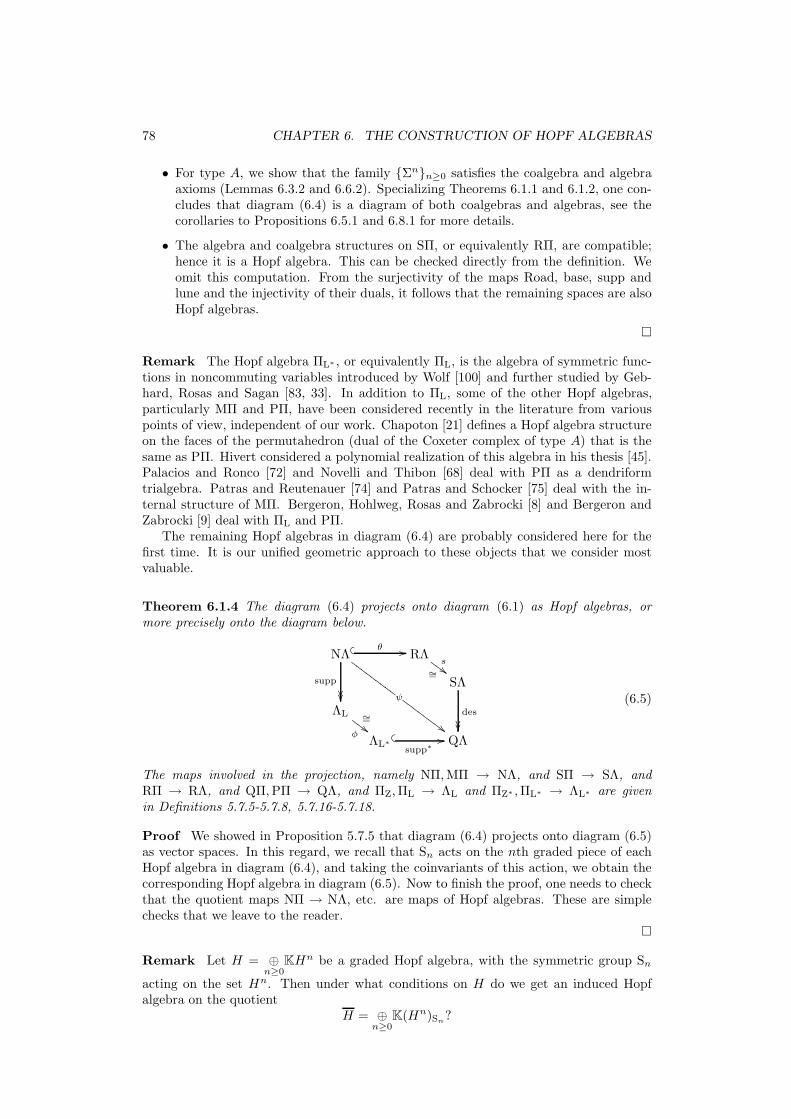
78 CHAPTER 6. THE CONSTRUCTION OF HOPF ALGEBRAS
• For type A, we show that the family {Σn}n≥0 satisfies the coalgebra and algebraaxioms (Lemmas 6.3.2 and 6.6.2). Specializing Theorems 6.1.1 and 6.1.2, one con-cludes that diagram (6.4) is a diagram of both coalgebras and algebras, see thecorollaries to Propositions 6.5.1 and 6.8.1 for more details.
• The algebra and coalgebra structures on SΠ, or equivalently RΠ, are compatible;hence it is a Hopf algebra. This can be checked directly from the definition. Weomit this computation. From the surjectivity of the maps Road, base, supp andlune and the injectivity of their duals, it follows that the remaining spaces are alsoHopf algebras.
�
Remark The Hopf algebra ΠL∗ , or equivalently ΠL, is the algebra of symmetric func-tions in noncommuting variables introduced by Wolf [100] and further studied by Geb-hard, Rosas and Sagan [83, 33]. In addition to ΠL, some of the other Hopf algebras,particularly MΠ and PΠ, have been considered recently in the literature from variouspoints of view, independent of our work. Chapoton [21] defines a Hopf algebra structureon the faces of the permutahedron (dual of the Coxeter complex of type A) that is thesame as PΠ. Hivert considered a polynomial realization of this algebra in his thesis [45].Palacios and Ronco [72] and Novelli and Thibon [68] deal with PΠ as a dendriformtrialgebra. Patras and Reutenauer [74] and Patras and Schocker [75] deal with the in-ternal structure of MΠ. Bergeron, Hohlweg, Rosas and Zabrocki [8] and Bergeron andZabrocki [9] deal with ΠL and PΠ.
The remaining Hopf algebras in diagram (6.4) are probably considered here for thefirst time. It is our unified geometric approach to these objects that we consider mostvaluable.
Theorem 6.1.4 The diagram (6.4) projects onto diagram (6.1) as Hopf algebras, ormore precisely onto the diagram below.
NΛ� � θ //
supp
���� ψGG
GGGG
GGG
##GGGGGGGG
RΛs
∼=##H
HH
SΛ
des
����ΛL
φ
∼=##F
FF
ΛL∗� �
supp∗// QΛ
(6.5)
The maps involved in the projection, namely NΠ,MΠ → NΛ, and SΠ → SΛ, andRΠ → RΛ, and QΠ,PΠ → QΛ, and ΠZ,ΠL → ΛL and ΠZ∗ ,ΠL∗ → ΛL∗ are givenin Definitions 5.7.5-5.7.8, 5.7.16-5.7.18.
Proof We showed in Proposition 5.7.5 that diagram (6.4) projects onto diagram (6.5)as vector spaces. In this regard, we recall that Sn acts on the nth graded piece of eachHopf algebra in diagram (6.4), and taking the coinvariants of this action, we obtain thecorresponding Hopf algebra in diagram (6.5). Now to finish the proof, one needs to checkthat the quotient maps NΠ → NΛ, etc. are maps of Hopf algebras. These are simplechecks that we leave to the reader.
�
Remark Let H = ⊕n≥0
KHn be a graded Hopf algebra, with the symmetric group Sn
acting on the set Hn. Then under what conditions on H do we get an induced Hopfalgebra on the quotient
H = ⊕n≥0
K(Hn)Sn?

6.2. THE HOPF ALGEBRAS OF TYPE A 79
The Hopf algebras in the above theorem, for example H = QΠ and H = QΛ, all fit inthis framework. Hence a good answer to this question can simplify matters a lot. Thisissue will be taken up in a future work.
In light of the theorems presented so far, one can ask the following question.
Open Question For a family {Σn}n≥0 of LRBs, can one define compatibility axiomssuch that if a family satisfies the coalgebra, algebra and compatibility axioms then dia-gram (6.3) is a diagram of Hopf algebras?
We make two comments about this question. Firstly, there must be enough exam-ples to justify an axiomatic approach; at the moment, there is only one example (Theo-rem 6.1.3). Secondly, we believe that the solution may require modification of the presentcoalgebra and algebra axioms themselves.
6.2 The Hopf algebras of type A
In this section, we define (without proof) the Hopf algebras in diagram (6.4). That is, wedo not check the (co)associativity of the (co)products or the compatibility of the productsand coproducts. These facts follow from the general considerations of later sections, seethe proof of Theorem 6.1.3 for a summary.
6.2.1 Summary
Table 6.2: Hopf algebras and their indexing sets.
Hopf algebras Indexing set
PΠ MΠ Σn = compositions of [n]
QΠ NΠ Qn = fully nested compositions of [n]
ΠL∗ ΠL Ln = partitions of [n]
ΠZ∗ ΠZ Zn = fully nested partitions of [n]
SΠ RΠ Cn × Cn = pairs of permutations of [n]
Table 6.3: Unified description of the Hopf algebras.
Hopf algebras Coproduct Product
PΠ, QΠ, ΠL∗ , ΠZ∗ Local vertex Quasi-shuffle
MΠ, NΠ, ΠL, ΠZ Global vertex Join
We showed in Section 5.4 that for the example of type A, the objects in diagram (6.3)can be described combinatorially, using the notions of (fully nested) set compositionsand partitions. Each one of them indexes two Hopf algebras, as shown in Table 6.2.We recall these four definitions in Sections 6.2.3, 6.2.6, 6.2.9 and 6.2.12, and for eachone define the notion of a local vertex, a global vertex, a quasi-shuffle and a join. Thegeometric meaning of the first two notions can be found in Tables 6.5 and 6.6. Withthese notions, the first eight Hopf algebras in Table 6.2 can be described in a unifiedway as summarized in Table 6.3. The formal definitions are given in Sections 6.2.4-6.2.5,6.2.7-6.2.8, 6.2.10-6.2.11, and 6.2.13-6.2.14. For example, the coproduct of PΠ, QΠ, ΠL∗

80 CHAPTER 6. THE CONSTRUCTION OF HOPF ALGEBRAS
and ΠZ∗ can be written using the notion of a local vertex of a composition, a fully nestedcomposition, a partition and a fully nested partition of [n] respectively, and so on. TheHopf algebras SΠ and RΠ are a little different and are defined towards the end of thissection (Sections 6.2.15-6.2.16).
6.2.2 The structure of the Hopf algebras of type A
Table 6.4: Hopf algebras and their structure.
Hopf algebra Comm. Cocomm. Structure
RΠ, SΠ No No Free and cofree
MΠ No Yes Free
PΠ No No Free and cofree
NΠ No No Free
QΠ No No Cofree
ΠL, ΠL∗ No Yes Free
ΠZ No No Free
ΠZ∗ No Yes
We now make a few comments about the structure of the Hopf algebras that weconstruct. Table 6.4 summarizes what is known so far. We note that the Hopf algebraMΠ is not dual to PΠ, the Hopf algebra ΠZ is not dual to ΠZ∗ ; similarly the Hopf algebraΠ (short for ΠL∗ and ΠL) is not self-dual. This is clear by looking at the commutativityand cocommutativity columns. This nonduality mystery will be explained in a futurework.
The fact that MΠ and NΠ, and Π and ΠZ are free follows directly from the definitionson the H and h basis respectively. The freeness and cofreeness of SΠ, or equivalently,RΠ, as well as the cofreeness of PΠ and QΠ will be proved in Chapter 7. The freenessof PΠ will be a consequence of further theory that we will develop in a follow-up to thiswork.
Remark The freeness and cofreeness of PΠ also appears in Bergeron and Zabrocki [9].Many other interesting Hopf algebras of a similar combinatorial nature are defined byHivert, Novelli and Thibon [45, 67, 68, 69, 44]. They are constructed as subalgebras of thefree algebra on countably many generators. This important point of view is not pursuedin this monograph. For other related work, see the references given in Section 6.1.3.
6.2.3 Set compositions
Definition 6.2.1 A vertex of a set N is an ordered splitting of N into two subsets. Ifone of the subsets is empty then we have a virtual vertex. For example,
134↓
25 ; 134 and 25
is a vertex of the set [5]. And↓
12345 and 12345↓
are the two virtual vertices of [5].
Definition 6.2.2 A set composition is an ordered set partition. For example, 6|34|125is a composition of [6].

6.2. THE HOPF ALGEBRAS OF TYPE A 81
Definition 6.2.3 There is a unique order preserving map st from any n-set N of theintegers to the standard n-set [n]. Using this map, one can standardize a composition ofN to a composition of [n]. For example,
st(9|36|58) = 5|13|24.
In the same way, we may standardize a composition of N to a composition of any n-set,say A, of the integers. We denote this map by stA.
Definition 6.2.4 A local vertex of a set composition F is an ordered splitting of F intotwo set compositions. For example,
F 1|F 2|F 3↓
|F 4; F 1|F 2|F 3 and F 4.
If one of the two set compositions is empty then we have a virtual local vertex. Everyset composition F has exactly two virtual local vertices.
F 1|F 2|F 3|F 4↓
; F 1|F 2|F 3|F 4 and ∅.
↓
F 1|F 2|F 3|F 4; ∅ and F 1|F 2|F 3|F 4.
Definition 6.2.5 A “shuffle” of set compositions F1 and F2 is a shuffle of the componentsof F1 and F2. For example,
5|mar|ce|21|34|lo|6 is a “shuffle” of 5|21|34|6 and mar|ce|lo.
This definition is not fully precise since we need to ensure that the shuffled sets aredisjoint. For that, we work with the following definition.
Let K = K1
↓
K2 be a vertex of the set N . And let F1 and F2 be compositions of thesets N1 and N2 such that |N1| = |K1| and |N2| = |K2|. Then a K-shuffle of F1 and F2 is
a shuffle of the components of stK1(F1) and stK2
(F2). For example, for K = 245679↓
138,
26|18|479|3|5 is a K-shuffle of 14|256|3 and 13|2.
We mostly deal with the special case when F1 and F2 are compositions of [g1] and [g2], andwe shuffle them by shifting the indices of F2 by g1 and then shuffling their components.
Definition 6.2.6 A “quasi-shuffle” of set compositions F1 and F2 is a shuffle of thecomponents of F1 and F2, where in addition we are allowed to substitute a disjoint set ofpairs of components (F i1 , F
j2 ) for F i1∪F
j2 , if they are adjacent in the shuffle. For example,
5sw|ap|21|34nil|6 is a “quasi-shuffle” of 5|21|34|6 and sw|ap|nil.
We leave it to the reader to make this precise by defining the notion of a K-quasi-shuffle,as in the previous definition.
Definition 6.2.7 A global vertex of a set composition P = P 1|P 2| · · · |P l is a choice ofa vertex for each set P i for 1 ≤ i ≤ l. This allows us to split P into two ordered setcompositions. For example,
12↓
5|347↓
|8↓
69 ; 12|347|8 and 5|69.
Note that there are two virtual global vertices that create an empty set composition aftersplitting.

82 CHAPTER 6. THE CONSTRUCTION OF HOPF ALGEBRAS
Definition 6.2.8 The join of a composition P1 of [g1] and a composition P2 of [g2] isthe composition j(P1 × P2) of [g1 + g2] obtained by shifting up the indices of P2 by g1and then placing it after P1. For example,
j(31|2× 23|14|5) = 31|2|56|47|8.
Remark The notion of a standardization map (Definition 6.2.3) and a virtual vertex(both local and global) exists and plays the same role for nested set compositions and(nested) set partitions also. We omit their definitions to avoid unnecessary repetition.Similarly, we do not repeat the issue of index shifting in the subsequent definitions ofquasi-shuffles.
6.2.4 The Hopf algebra PΠ
Let PΠ = ⊕n≥0
K(Σn)∗, where Σn is the set of compositions of [n]. Write MF for the basis
element corresponding to F ∈ Σn, n > 0 and 1 for the basis element of degree 0.
Definition 6.2.9 The coproduct on PΠ is given by
∆(MF ) =∑
local vertices of F
MF1⊗MF2
. (6.6)
A local vertex, by definition, splits F into two ordered parts. The F1 and F2 in the aboveformula are obtained by standardizing these two parts respectively. The two virtual localvertices of F contribute to the terms 1⊗MF and MF ⊗ 1. More explicitly,
∆(MF 1|···|F l) =
l∑
i=0
Mst(F 1|···|F i) ⊗Mst(F i+1|···|F l).
For example,
∆(M136|25|47) = 1⊗M136|25|47 +M123 ⊗M13|24 +M135|24 ⊗M12 +M136|25|47 ⊗ 1.
Definition 6.2.10 The product on PΠ is given by
MF1∗MF2
=∑
F : F a quasi-shuffle of F1 and F2
MF . (6.7)
If F1 and F2 are compositions of [g1] and [g2] respectively then the understanding is thatwe shift up the indices of F2 by g1 and then quasi-shuffle. For example,
M13|2 ∗M12 = M13|2|45 +M13|45|2 +M45|13|2 +M13|245 +M1345|2.
These formulas for the product and coproduct agree with Formulas (1) and (2) ofChapoton [21].
6.2.5 The Hopf algebra MΠ
Let MΠ = ⊕n≥0
KΣn, where Σn is the set of compositions of [n]. Write HP for the basis
element corresponding to P ∈ Σn, n > 0 and 1 for the basis element of degree 0.
Definition 6.2.11 The coproduct on MΠ is given by
∆(HP ) =∑
global vertices of P
HP1⊗HP2
. (6.8)

6.2. THE HOPF ALGEBRAS OF TYPE A 83
A global vertex splits P into two ordered parts. The P1 and P2 in the above formula areobtained by standardizing these two parts respectively. The two virtual global verticesof P contribute to the terms 1⊗HP and HP ⊗ 1. For example,
∆(H1|2|3) = 1⊗H1|2|3 + 3(H1 ⊗H1|2 +H1|2 ⊗H1) +H1|2|3 ⊗ 1.
The global vertices 1↓
|↓
2|↓
3,↓
1|2↓
|↓
3,↓
1|↓
2|3↓
each give the term H1 ⊗ H1|2, the global
vertices 1↓
|2↓
|↓
3,↓
1|2↓
|3↓
, 1↓
|↓
2|3↓
each give the term H1|2 ⊗ H1, and the two virtualglobal vertices give the end terms.
In contrast to the local case, different global vertices of P can give rise to the sameP1 and P2.
Remark The Hopf algebra MΠ is cocommutative.
5↓
12|3↓
74|689↓
; 5|3|689 and 12|74.
12↓
5|74↓
3|↓
689 ; 12|74 and 5|3|689.
As illustrated above, there is an involution without fixed points on the set of globalvertices of P obtained by switching the order of the two parts in each component of P . Ifa global vertex K splits P into P1 and P2 then K, the image of K under the involution,splits P into P2 and P1. This shows that MΠ is cocommutative.
Definition 6.2.12 The product on MΠ is given by
HP1∗HP2
= Hj(P1×P2). (6.9)
For example,
H31|2 ∗H12 = H13|2|45.
6.2.6 Nested set compositions
Definition 6.2.13 A nested set composition is a sequence F = F 1|F 2| . . . |F l, in which
each F i is a set composition of Ai, and A1| . . . |Al is a set composition of [n]. For example,
(3|15|7|48|29|6)
is a nested composition of [9]. A fully nested set composition is a nested set compositionwith singleton blocks.
Equivalently, a nested set composition is a pair (F,H) of set compositions such thatF ≤ H . In the above example, the pair is (135|24789|6, 3|15|7|48|29|6). And a fullynested set composition is a pair (F,D) with F ≤ D and D a chamber.
We use both the notations depending on our convenience.
Definition 6.2.14 A local vertex of a nested set composition (F,H) is simply a localvertex of F , as given in Definition 6.2.4. For example,
3|15
↓
|7|48|29|6 ; 3|15 and 7|48|29|6.
In other words, a local vertex is either a choice of a big bar, or one of the two extremechoices on either side corresponding to the virtual local vertices.

84 CHAPTER 6. THE CONSTRUCTION OF HOPF ALGEBRAS
Definition 6.2.15 A quasi-shuffle of two fully nested set compositions (F1, D1) and(F2, D2) is a fully nested set composition (F,D), where F is a quasi-shuffle of F1 and F2
and D is the underlying shuffle of D1 and D2. For example,
3|1|b|a|c|5|4|2|d|6 is a quasi-shuffle of 3|1|5|4|2|6 and b|a|c|d.In other words, we quasi-shuffle with respect to the big bars, and if two blocks get mergedin the quasi-shuffle then we write them one after the other with a small bar in between.
Definition 6.2.16 A global vertex of a fully nested set composition P 1|P 2| . . . |P l is a
choice of a local vertex for each set composition P i. This allows us to split P into twoordered fully nested set compositions. For example,
3↓
|1|5|4↓
|2|7|↓
6|8 ; 3|5|4 and 1|2|7|6|8.
Definition 6.2.17 The join of a nested set composition (P1, Q1) of [g1] and a nested setcomposition (P2, Q2) of [g2] is the nested set composition of [g1 + g2] given by (j(P1 ×P2), j(Q1 ×Q2)), with the notation as in Definition 6.2.8. For example,
j(3|1|2× 23|1|4|5) = 3|1|2|56|4|7|8.
Remark Note that we defined a quasi-shuffle and global vertex only for fully nestedset compositions. These notions for nested set compositions are more complicated. Sincethey are not necessary for this chapter, we omit them.
6.2.7 The Hopf algebra QΠ
Let QΠ = ⊕n≥0
K(Qn)∗, where Qn is the set of fully nested compositions of [n]. Write
M(F,D) for the basis element corresponding to (F,D) ∈ Qn, n > 0 and 1 for the basiselement of degree 0.
Definition 6.2.18 The coproduct and product on QΠ are given by Equations (6.6)and (6.7), but where local vertex and quasi-shuffle are now given by Definitions 6.2.14and 6.2.15. As an example, for the coproduct,
∆(M3|1|5|4|2|6) = 1⊗M
3|1|5|4|2|6 +M3|1|5 ⊗M2|1|3 +M
3|1|5|4|2 ⊗M1 +M3|1|5|4|2|6 ⊗ 1.
The number of terms is two more than the number of big bars in the nested set compo-sition.
As an example, for the product,
M2|3|1|4 ∗M2|1 = M
2|3|1|4|6|5 +M2|3|6|5|1|4 +M
6|5|2|3|1|4 +M2|3|1|4|6|5 +M
2|3|6|5|1|4.
6.2.8 The Hopf algebra NΠ
Let NΠ = ⊕n≥0
KQn, where Qn is the set of fully nested compositions of [n]. Write H(P,C)
for the basis element corresponding to (P,C) ∈ Qn, n > 0 and 1 for the basis element ofdegree 0.
Definition 6.2.19 The coproduct and product on NΠ are given by Equations (6.8)and (6.9), but where global vertex and join are now given by Definitions 6.2.16 and 6.2.17.For example, for the coproduct,
∆(H3|1|2) = 1⊗H
3|1|2 +H1 ⊗H2|1 +H1 ⊗H1|2 +H
2|1 ⊗H1 +H2|1 ⊗H1 +H3|1|2 ⊗ 1.

6.2. THE HOPF ALGEBRAS OF TYPE A 85
The fully nested set composition 3|1|2 has 3 ∗ 2 = 6 global vertices, namely,
↓
3|1|↓
2 ,↓
3|1|2↓
, 3↓
|1|↓
2 , 3↓
|1|2↓
, 3|1↓
|↓
2 , 3|1↓
|2↓
.
Each one of these contributes to a term in the coproduct.The product is quite simple and involves only one term. For example,
H2|3|1|4 ∗H2|1 = H
2|3|1|4|6|5.
6.2.9 Set partitions
We denote a set partition by X = {X1, X2, . . . , X l}. For example, {134, 56, 2} is apartition of the set [6].
Definition 6.2.20 A local vertex of a set partition X is an ordered splitting of X intotwo set partitions. For example,
{X1, X2, X3, X4} ; {X1, X2, X4} and {X3}.
Definition 6.2.21 A quasi-shuffle of set partitions X1 and X2 is the union of X1 andX2, where in addition we are allowed to substitute a disjoint set of pairs of components(X i
1, Xj2) for X i
1 ∪Xj2 . For example,
{34a, 15bd, 6, c} is a quasi-shuffle of {15, 34, 6} and {a, bd, c}.
Definition 6.2.22 A global vertex of a set partition Y = {Y 1, Y 2, . . . , Y l} is a choiceof a vertex for each set Y i. For example,
{36↓
4, 7↓
1, 2↓
5} ; {36, 7, 2} and {4, 1, 5}.
Definition 6.2.23 The join of a partition Y1 of [g1] and a partition Y2 of [g2] is apartition j(Y1 × Y2) of [g1 + g2] obtained by shifting up the indices of Y2 by g1 and thentaking union with Y1. For example,
j({31, 2} × {23, 14, 5}) = {31, 2, 56, 47, 8}.
6.2.10 The Hopf algebra ΠL∗
Let ΠL∗ = ⊕n≥0
K(Ln)∗, where Ln is the set of partitions of [n]. Write mX for the basis
element corresponding to X ∈ Ln, n > 0 and 1 for the basis element of degree 0.
Definition 6.2.24 The coproduct and product on ΠL∗ are given by Equations (6.6)and (6.7), but where local vertex and quasi-shuffle are now given by Definitions 6.2.20and 6.2.21. As an example, for the coproduct,
∆(m{13,2}) = 1⊗m{13,2} +m{12} ⊗m{1} +m{1} ⊗m{12} +m{13,2} ⊗ 1.
As an example, for the product,
m{13,2} ∗m{12} = m{13,2,45} +m{13,245} +m{1345,2}.
It is clear that the coproduct is cocommutative.

86 CHAPTER 6. THE CONSTRUCTION OF HOPF ALGEBRAS
6.2.11 The Hopf algebra ΠL
Let ΠL = ⊕n≥0
KLn, where Ln is the set of partitions of [n]. Write hY for the basis element
corresponding to Y ∈ Ln, n > 0 and 1 for the basis element of degree 0.
Definition 6.2.25 The coproduct and product on ΠL are given by Equations (6.8)and (6.9), but where global vertex and join are now given by Definitions 6.2.22 and 6.2.23.For example, for the coproduct,
∆(h{12,3}) = 1⊗ h{12,3} + 2(h{1} ⊗ h{1,2} + h{1,2} ⊗ h{1})+
(h{1} ⊗ h{12} + h{12} ⊗ h{1}) + h{12,3} ⊗ 1.
The product is quite simple and involves only one term. For example,
h{134,2} ∗ h{1,23} = h{134,2,5,67}.
Note that using the reasoning given for MΠ, it follows that the coalgebra ΠL is alsococommutative. We may also use the fact that the quotient of a cocommutative coalgebrais again cocommutative. As mentioned before, this Hopf algebra is not self-dual.
Remark The Hopf algebras ΠL and ΠL∗ are isomorphic. This is a part of the claimmade in Theorem 6.1.3.
6.2.12 Nested set partitions
Definition 6.2.26 A nested set partition is a set L = {L1, . . . , Ll}, in which each Li isa set composition of Ai, and {A1, . . . , Al} is a set partition of [n]. For example,
{3|56, 2|17, 4}
is a nested partition of [7]. A fully nested set partition is a nested set partition withsingleton blocks.
Definition 6.2.27 A local vertex of a nested set partition L is an ordered splitting of Linto two nested set partitions. For example,
{L1, L2, L3, L4} ; {L1, L2, L4} and {L3}.
Definition 6.2.28 A quasi-shuffle of two fully nested set partitions L1 and L2 is a unionof L1 and L2, where in addition we are allowed to substitute a disjoint set of pairs ofcomponents (Li1, L
j2) for the composition Li1|L
j2. For example,
{3|4|a, 1|6|c|d, b, 2|7} is a quasi-shuffle of {1|6, 3|4, 2|7} and {a, c|d, b}.
Definition 6.2.29 A global vertex of a fully nested set partition M = {M1, . . . ,M l} isa choice of a local vertex for each set composition M i. For example,
{↓
3|6|4, 7|8|1↓
|9, 2↓
|5} ; {7|8|1, 2} and {3|6|4, 9, 5}.
Definition 6.2.30 The join of nested partitions M1 of [g1] and M2 of [g2] is a nestedpartition j(M1 ×M2) of [g1 + g2] obtained by shifting up the indices of M2 by g1 andthen taking union with M1. For example,
j({3|1, 2} × {23, 1|4, 5}) = {3|1, 2, 56, 4|7, 8}.
Remark As for nested set compositions, to avoid complications, we have defined aquasi-shuffle and global vertex only for fully nested set partitions.

6.2. THE HOPF ALGEBRAS OF TYPE A 87
6.2.13 The Hopf algebra ΠZ∗
Let ΠZ∗ = ⊕n≥0
K(Zn)∗, where Zn is the set of fully nested partitions of [n]. Write mL for
the basis element corresponding to L ∈ Zn, n > 0 and 1 for the basis element of degree0.
Definition 6.2.31 The coproduct and product on ΠZ∗ are given by Equations (6.6)and (6.7), but where local vertex and quasi-shuffle are now given by Definitions 6.2.27and 6.2.28. As an example, for the coproduct,
∆(m{1|3,4|2}) = 1⊗m{1|3,4|2} +m{1|2} ⊗m{2|1} +m{2|1} ⊗m{1|2} +m{1|3,4|2} ⊗ 1.
As an example, for the product,
m{1|4|3,2} ∗m{1|2} = m{1|4|3,2,5|6} +m{1|4|3,2|5|6} +m{1|4|3|5|6,2}.
It is clear that the coproduct is cocommutative.
6.2.14 The Hopf algebra ΠZ
Let ΠZ = ⊕n≥0
KZn, where Zn is the set of fully nested partitions of [n]. Write hM for the
basis element corresponding to M ∈ Zn, n > 0 and 1 for the basis element of degree 0.
Definition 6.2.32 The coproduct and product on ΠZ are given by Equations (6.8)and (6.9), but where global vertex and join are now given by Definitions 6.2.29 and 6.2.30.For example,
∆(h{3|1,2}) = 1⊗ h{3|1,2} + h{1} ⊗ h{2|1} + h{2|1} ⊗ h{1}
+h{1} ⊗ h{1,2} + h{1,2} ⊗ h{1} + h{3|1,2} ⊗ 1.
The product is quite simple and involves only one term. For example,
h{1|4|3,2} ∗ h{1,2|3} = h{1|4|3,2,5,6|7}.
Remark The Hopf algebras ΠZ and ΠZ∗ are neither isomorphic nor dual to each other.
6.2.15 The Hopf algebra SΠ
Let SΠ = ⊕n≥0
K(Cn × Cn)∗, where Cn are the chambers in Σn and can be identified with
permutations. Write F(C,D) for the basis element (C,D) ∈ Cn × Cn, n > 0 and 1 for thebasis element of degree 0. Let C = C1|C2| . . . |Cn and D = D1|D2| . . . |Dn.
Definition 6.2.33 The coproduct on SΠ is given by
∆(F(C,D)) =n∑
i=0
Fst(C1|···|Ci,D1|···|Di) ⊗ Fst(Ci+1|···|Cn,Di+1|···|Dn),
where C1, . . . , Ci are the letters in the set {D1, . . . , Di} and Ci+1, . . . , Cn are the lettersin the set {Di+1, . . . , Dn} written in the order in which they appear in C1| · · · |Cn. Forexample,
∆(F2|3|1|4,4|2|1|3) = 1⊗ F2|3|1|4,4|2|1|3 + F1,1 ⊗ F2|3|1,2|1|3 + F1|2,2|1 ⊗ F2|1,1|2+
F2|1|3,3|2|1 ⊗ F1,1 + F2|3|1|4,4|2|1|3 ⊗ 1.

88 CHAPTER 6. THE CONSTRUCTION OF HOPF ALGEBRAS
Definition 6.2.34 The product on SΠ is given by
F(C1,D1) ∗ F(C2,D2) =∑
D: D a shuffle of D1 and D2
F(j(C1×C2),D).
The term j(C1 ×C2) refers to the join of C1 and C2 given in Definition 6.2.8. If D1 andD2 are compositions of [g1] and [g2] respectively then the understanding is that we shiftup the indices of D2 by g1 and then shuffle. For example,
F(2|1,2|1) ∗ F(2|1,1|2) = F(2|1|4|3,2|1|3|4) + F(2|1|4|3,2|3|1|4) + F(2|1|4|3,3|2|1|4)+
F(2|1|4|3,2|3|4|1) + F(2|1|4|3,3|2|4|1) + F(2|1|4|3,3|4|2|1).
6.2.16 The Hopf algebra RΠ
Let RΠ = ⊕n≥0
K(Cn × Cn), where Cn are the chambers in Σn and can be identified with
permutations. Write K(D,C) for the basis element (D,C) ∈ Cn × Cn, n > 0 and 1 for thebasis element of degree 0. We define a product and coproduct on RΠ (see below) suchthat:
Proposition 6.2.1 The switch map s : RΠ → SΠ which sends K(D,C) → F(C,D) is anisomorphism of Hopf algebras.
Definition 6.2.35 The coproduct on RΠ is given by
∆(K(D,C)) =
n∑
i=0
Kst(D1|···|Di,C1|···|Ci) ⊗Kst(Di+1|···|Dn,Ci+1|···|Cn).
where C1, . . . , Cn are as in Definition 6.2.33.
Definition 6.2.36 The product on RΠ is given by
K(D1,C1) ∗K(D2,C2) =∑
D: D a shuffle of D1 and D2
K(D,j(C1×C2)).
Remark As mentioned above, the Hopf algebras RΠ and SΠ are clearly isomorphic.However for book-keeping purposes, we prefer to keep them separate.
6.3 The coalgebra axioms and examples
In this section, we give the coalgebra axioms for a family of posets (Section 6.3.1). Theyappear very abstract at first glance; however they are natural, that is, there are manyexamples (Sections 6.3.2-6.3.4). The motivation is that one can construct the coalgebrasin diagram (6.3) starting with a family of posets that satisfies these axioms.
Our first example (Section 6.3.2) is based on compositions. It is simple yet nontrivialenough to help the reader gain some understanding of the axioms. The next example(Section 6.3.3) arises from the Coxeter group of type A. It is the motivating examplewhich led us to the axioms. We give two viewpoints for this example, one geometric andthe other combinatorial, stressing the former. In Section 6.3.4, we give another examplefrom Coxeter theory.

6.3. THE COALGEBRA AXIOMS AND EXAMPLES 89
6.3.1 The coalgebra axioms
Consider the family {Σn}n≥0, where Σn is a finite graded poset of rank n − 1 with aunique minimum element that we denote ∅. Further let Σ0 and Σ1 be singleton sets withthe unique element ∅. For K a face of Σ, let
ΣnK = {F ∈ Σn | K ≤ F}.
Let Cn be the set of chambers (maximal elements) in Σn and CnF = {D ∈ Cn | F ≤ D}.Let degK = rankK + 1, where rank denotes the rank of an element.
We give three coalgebra axioms for such a family of posets.
Axiom (C1). For every face F of Σn, there exists a composition (f1, f2, . . . , fdegF ) of nand a poset isomorphism
bF : ΣnF → Σf1 × Σf2 × . . .× Σfdeg F . (6.10)
For F = ∅, the composition is (n) and the poset isomorphism b∅ is the identity mapid : Σn → Σn.
GFED@ABCbF
66lllllllll //
((RRRRRRRRR
Figure 6.1: The break map bF .
Figure 6.1 shows a schematic picture for the break map bF for degF = 3. The circleat the center is an apparatus which takes one input larger than F and produces threeordered outputs.
Axiom (C2). The maps bF in axiom (C1) are “associative” in the following sense.Let K be a face of F . First apply the axiom (C1) to the face K of Σn to get a
composition (k1, k2, . . . , kdegK) of n and a poset isomorphism
bK : ΣnK → Σk1 × Σk2 × . . .× Σkdeg K .
Under this map, let F 7→ F1 × F2 × . . .× FdegK . This induces an isomorphism
bK : ΣnF → Σk1F1× Σk2F2
× . . .× Σkdeg K
Fdeg K.
Apply the axiom (C1) to the face Fi of Σki to get a composition (fi1, fi2, . . . , fidegFi) of
ki and a poset isomorphism
bFi: Σki
Fi→ Σfi1 × Σfi2 × . . .× Σfideg Fi for 1 ≤ i ≤ degK.
Then, we havebF = (bF1
× bF2× . . .× bFdeg K
) ◦ bK , (6.11)
where bF is the poset map given by the axiom (C1) for the face F . In particular, werequire that
(f1, f2, . . . , fdegF ) = (f11, f12, . . . , f1degF1, f21, . . . , fmdegFm
), (6.12)
where m = degK.Figure 6.2 shows a schematic picture for the associativity of the break map. It sum-
marizes what is going on without using the above menagerie of symbols.
Axiom (C3). Every rank 2 face H of Σn has exactly two rank 1 faces, say K and G.Further the poset isomorphisms bK : ΣnK → Σk1 ×Σk2 and bG : ΣnG → Σg1 ×Σg2 map Hto ∅ ×K ′ and G′ × ∅ respectively for some rank 1 faces K ′ ∈ Σk2 and G′ ∈ Σg1 .

90 CHAPTER 6. THE CONSTRUCTION OF HOPF ALGEBRAS
GFED@ABCbF1
rrrr
88rrr
&&LLL
GFED@ABCbK
99rrrr//
%%LLLL
GFED@ABCbF2//
GFED@ABCbF3
LLLL 88rrr
&&LLL
= ONMLHIJKbF
66mmmmmmmmm
??~~~~~~~~
((QQQQQQQQQ
@@@
@@@@
@//
Figure 6.2: The break map is associative.
Remark The content of this axiom is not the existence of K ′ and G′ but the fact thatthey belong to the second and first coordinate respectively of the range.
In addition to the above three coalgebra axioms, we define a projection axiom. Forthat assume, in addition, that each Σn is a projection poset, as defined in Section 2.7.This includes the case when Σn is a LRB.
Axiom (CP ). The poset maps respect the product structure of Σn; that is, for anyF ≤ H,N ∈ Σn, we have
bF (HN) = bF (H)bF (N),
where bF is the poset isomorphism associated to F by the axiom (C1).
Remark The elements of rank 1, or equivalently, degree 2 in Σn have a special roleto play when we consider coproducts. We also refer to them as vertices, since Σn is asimplicial complex in our examples.
Proposition 6.3.1 Let {Σn}n≥0 satisfy the coalgebra axioms (C1) and (C2). Then foreach n > 0, there are poset maps
type : Σn → Qn,
where Qn
is the poset of compositions of n.
Proof The map type sends a face F ∈ Σn to the composition (f1, f2, . . . , fdegF ) of nas given by the axiom (C1). The axiom (C2), in particular Equation (6.12), implies thatthis is a poset map.
�
Remark In our examples, the map type : Σn → Qn
is a map from a simplicial complexof rank n− 1 to the simplex of rank n− 1. It will always be surjective and have a “nice”section Q
n→ Σn. This section is important for the algebra axioms that we consider in
Section 6.6.
6.3.2 The warm-up example of compositions
Let Σn = Qn
be the simplex of rank n − 1, n ≥ 0. As a poset, it consists of subsets of[n− 1], or equivalently, compositions of n. Recall that a composition of n of degree l is a
sequence α = (α1, . . . , αl) of positive integers such that∑li=1 αi = n. The partial order
of Qn
is given by subset inclusion, or equivalently, refinement of compositions. The posetQn
has only one chamber D, namely the n-tuple
(1, 1, . . . , 1︸ ︷︷ ︸n
)

6.3. THE COALGEBRA AXIOMS AND EXAMPLES 91
and a unique minimum element ∅ = (n). It is a commutative LRB with the productbeing union of subsets. Let
Qn
α = {β ∈ Qn| α ≤ β}.
Our goal is to show the following.
Lemma 6.3.1 The family of LRBs {Qn}n≥0 satisfies all coalgebra axioms (C1)− (CP ).
Proof The map in Proposition 6.3.1, in this case, is the identity isomorphism Qn→ Q
n.
So the situation is as simple as can be. The break map is defined as below.
Definition 6.3.1 For α = (α1, . . . , αk), a composition of n and degree k, we define aposet isomorphism
bα : Qn
α → Qα1×Q
α2× . . .×Q
αk
as follows.
Let β ∈ Qn
α be a refinement of α. Then the image of β on the ith factor is obtained bylumping together the parts of β that refine αi. For example, for n = 9 and α = (2, 4, 3),
the map Q9
α → Q2×Q
4×Q
3sends β = (2, 1, 3, 2, 1) to (2)× (1, 3)× (2, 1).
It is easy but instructive to check the axioms (C2) and (CP ) from this definition.This is left to the reader. We check the axiom (C3). Let α = (α1, α2, α3) be a rank 2face. Then it has two rank 1 faces, namely, β = (α1, α2 + α3) and γ = (α1 + α2, α3).
Further, the maps Qn
β → Qα1×Q
α2+α3and Q
n
γ → Qα1+α2
×Qα3
send α to (α1)×(α2, α3)and (α1, α2)× (α3) respectively, in accordance with the axiom (C3). Remember that (n)stands for the empty face ∅ in Q
n.
�
Remark The idea behind Definition 6.3.1 is better seen in the language of subsets. Itwill also be useful for the next example. Let V be a subset of [n− 1] of cardinality k− 1.Then
[n− 1] \ V =
k⊔
j=1
Ij
is a disjoint union of k intervals. To every T such that V ⊆ T ⊆ [n−1], one can associateTj ⊆ Ij by the identity
T = V⊔
k⊔
j=1
Tj
. (6.13)
This defines a poset isomorphism
Qn
V −→k×j=1{subsets of Ij},
equivalent to the one in Definition 6.3.1, that sends T to T1 × T2 × . . .× Tk.
6.3.3 The motivating example of type An−1
The motivation for the coalgebra axioms comes from the theory of Coxeter groups. Let(W,S) be a Coxeter system, Σ its Coxeter complex and C the set of chambers in Σ. Werecall some key facts from Chapters 1 and 2.

92 CHAPTER 6. THE CONSTRUCTION OF HOPF ALGEBRAS
Fact 6.3.1 A Coxeter complex Σ is a left regular band (LRB). For F ∈ Σ and C ∈ C,the chamber FC is that chamber in CF = {D | F ≤ D} which is closest in the gallerymetric to C. This is shown in Figure 1.2. The product in Σ is then given by
FP =⋂
P≤C
FC.
We call FP the projection of P on F .
Fact 6.3.2 Let F ∈ Σ be a face of type T ≤ S. Then the link of F in Σ, denotedlink(F ), is again a Coxeter complex. In our notation, link(F ) ∼= ΣF as posets. Furtherthe Coxeter diagram of link(F ) is obtained from the Coxeter diagram of Σ by deletingall the vertices whose type is contained in T .
Fact 6.3.3 The join Σ1∗Σ2 of two Coxeter complexes is again a Coxeter complex, whosediagram is the disjoint union of the diagrams of Σ1 and Σ2. Further, the join operationis compatible with the projection maps, that is,
(H1 ∗N1)(H2 ∗N2) = (H1H2 ∗N1N2), where Hi, Ni ∈ Σi.
Geometry
Recall from Section 1.4 that for type An−1, the Coxeter group W is Sn, the symmetricgroup on n letters and S = {s1, . . . , sn−1}, where si is the transposition that interchangesi and i+1. Let Σn be the Coxeter complex of Sn. Identify Q
n, the poset of compositions
of n under refinement, with the poset of subsets of S under inclusion in the usual way.
��������s1
��������s2
. . . ��������sn−1
Figure 6.3: The Coxeter diagram of type An−1.
Lemma 6.3.2 The family of LRBs {Σn}n≥0 satisfies all coalgebra axioms (C1)− (CP ).
Proof Our goal here is two-fold, to prove the above lemma; at the same time, to usethis example, to motivate the axioms themselves.
Axiom (C1). Let F ∈ Σ be a face of type T ≤ S. Observe that deleting |T | = rankFvertices breaks the Coxeter diagram of type A, shown in Figure 6.3, into
degF = rankF + 1,
possibly empty, disjoint parts, each part again being of type A. Further, these parts canbe ordered in a natural way. In other words, using Facts 6.3.2 and 6.3.3,
bF : ΣnF∼=−→ Σf1 × Σf2 × . . .× Σfdeg F , (6.14)
where fi = 1+ (number of vertices in the ith part) and where × refers to the join ofsimplicial complexes. It is the cartesian product at the level of posets. This is the originof the coalgebra axiom (C1). There is still one difference though. The above isomorphismbF is specified only upto the symmetric groups involved. To pick out a specific bF , oneneeds to do the following.

6.3. THE COALGEBRA AXIOMS AND EXAMPLES 93
Fix a fundamental chamber Cn0 in Σn for all n ≥ 1. Now define bF to be the uniqueisomorphism that maps
FCn0 7→ Cf10 × C
f20 × . . .× C
fdeg F
0 . (6.15)
In this case, Proposition 6.3.1 specializes to the following.
Proposition 6.3.2 The poset map type : Σn → Qn
sends F ∈ Σn to type(F ) ≤ S.
This explains the origin of the name “type”. The above map is clearly surjective andhas a “nice” section that sends T ≤ S to the face of the fundamental chamber Cn0 of typeT .
Axiom (CP ). With bF as defined in Equation (6.14), it follows from Fact 6.3.3 that{Σn}n≥0 satisfies the axiom (CP ).
Axiom (C2). We now show that {Σn}n≥0 satisfies the axiom (C2). In other words,we show that Equation (6.11) holds. We use the notation of the axioms (C1) and (C2),and further set m = degK for notational simplicity. The first requirement is that Equa-tion (6.12) holds.
To get the composition of n in the left hand side of Equation (6.12) , we delete thosevertices from the Coxeter diagram of Σn whose type is contained in type(F ). And toget the composition of n in the right hand side, we first delete those vertices whose typeis contained in type(K) and then from the ith part delete those vertices whose type iscontained in type(Fi), for 1 ≤ i ≤ m. The point is that in both cases we delete the samevertices because
type(F ) = type(K)⊔
m⊔
j=1
type(Fj)
. (6.16)
since bK(F ) = F1 × F2 × . . .× Fm. This proves Equation (6.12). It is also instructive tocompare Equations (6.16) and (6.13).
Hence both sides of Equation (6.11) specify an isomorphism
ΣnF → Σf11 × Σf12 × . . .Σf1deg F1 × Σf21 × . . .× Σfm deg Fm .
To see that they specify the same isomorphism, one needs to check that
bF (FCn0 ) = (bF1× bF2
× . . .× bFm) ◦ bK(FCn0 ). (6.17)
For the left hand side, by (6.15), we have
bF (FCn0 ) = Cf110 × Cf120 × . . . C
f1deg F1
0 × Cf210 × . . .× Cfm deg Fm
0 .
The right hand side requires more work. Since K ≤ F , we have FCn0 = FKCn0 . Hence,first by the axiom (CP ), which we proved, and then applying (6.15) to bK , we obtain
bK(FCn0 ) = bK(F )bK(KCn0 ) = F1Ck10 × F2C
k20 × . . .× FmC
km
0 .
Applying (bF1× bF2
× . . .× bFm) to both sides and applying (6.15) to each bFi
, we obtain
(bF1× bF2
× . . .× bFm) ◦ bK(FCn0 ) = C
f110 ×Cf120 × . . . C
f1deg F1
0 ×Cf210 × . . .×Cfm deg Fm
0 .
This proves Equation (6.17) and consequently the axiom (C2).
Axiom (C3). Note that Σn is a simplicial complex. Hence, a rank 2 face H in an edgein Σn and has 2 rank 1 faces, or vertices, say K and G. If type(H) = {si, sj} withi < j then assume for concreteness that K has type si and G has type sj . Note thatif we delete the vertex of type si (resp. sj) then the Coxeter diagram of Σn, shown inFigure 6.3, breaks into two ordered parts with sj (resp. si) in the second (resp. first)part. This is the content of the axiom (C3).
�

94 CHAPTER 6. THE CONSTRUCTION OF HOPF ALGEBRAS
Combinatorics
We now explain the combinatorial content of the geometry. The Coxeter complex Σn
can be identified with Bn, the poset of set compositions. Namely, the elements of Bn arecompositions F = F 1| . . . |F l of the set [n]. For example, 347|16|258 is an element of B8.The equivalence between the geometry and the combinatorics is explained in detail inSection 1.4, with further details in Section 5.4.
Definition 6.3.2 Multiply two set compositions by taking intersections and orderingthem lexicographically; more precisely, if F = F 1| . . . |F l and H = H1| . . . |Hm, then
FH = (F 1 ∩H1| . . . |F 1 ∩Hm| . . . |F l ∩H1| . . . |F l ∩Hm) ,
where the hat means “delete empty intersections”. For example,
(347|16|258)(6|157|28|34) = (7|34|6|1|5|28).
For the partial order of Bn, we say F ≤ H if H is a refinement of F . The minimumelement in Bn is the one block partition 12 . . . n. An element of rank 1 in Bn is a two blockordered partition F 1|F 2 of [n]. The set of chambers Cn in Σn consists of set compositionswith singleton blocks, so they correspond to permutations of [n].
Lemma 6.3.3 The family of LRBs {Bn}n≥0 satisfies all coalgebra axioms (C1)− (CP ).
In principle, we already proved this in Lemma 6.3.2. So what is happening is lan-guage translation. For the fundamental chamber Cn0 in Σn, we take the set composition1|2| . . . |n. The geometric procedure then yields the following.
Definition 6.3.3 For F = F 1| . . . |F l, a composition of the set [n], we have l = degF .Let fi be the cardinality of F i for 1 ≤ i ≤ l. The poset isomorphism
bF : BnF → Bf1 × Bf2 × . . .× Bfl
is defined as follows.
LetH ∈ BnF be a refinement of F . Then the image ofH on the ith factor is obtained bylumping together the blocks of H that refine F i and standardizing (see Definition 6.2.3)so that the result is a composition of the set [fi].
For example, for n = 9 and F = 18|2357|469, the map bF : B9F → B
2×B4×B3 sendsH = 18|5|3|27|9|46 to the triplet 12× 3|2|14× 3|12.
The combinatorial content of Proposition 6.3.2 is the following.
Proposition 6.3.3 The poset map type : Bn ։ Qn, sends a composition of the set [n]
to its underlying composition of n.
The “nice” section Qn→ Bn sends a composition (α1, α2, . . . , αk) of n to the set com-
position
12 . . . α1|α1 + 1 . . . α1 + α2| . . . | . . . n.
We know from Lemma 6.3.2 that the axioms (C2) − (CP ) hold. But it is fun andinstructive to check them directly using Definitions 6.3.2 and 6.3.3. For example, tocheck the axiom (C3), let H = H1|H2|H3 be a rank 2 face. As a concrete example, takeH = 136|25|47. Then its two rank 1 faces are K = 136|2457 and G = 12356|47. Themap bK maps H to 123× 13|24 and bG maps H to 135|24× 12. Remember that 123 and12 are the empty faces in Σ3 and Σ2 respectively.

6.3. THE COALGEBRA AXIOMS AND EXAMPLES 95
6.3.4 The example of type A×(n−1)1
Geometry
Recall from Section 5.5 that for type A×(n−1)1 , the Coxeter group is Z
n−12 and S =
{s1, . . . , sn−1}, where si is the generator in the ith coordinate. Let Σn be the Coxetercomplex of Z
n−12 . Its Coxeter diagram is shown in Figure 6.4. Identify Q
n, the poset of
compositions of n under refinement, with the poset of subsets of S under inclusion in theusual way.
��������s1
��������s2
. . . ��������sn−1
Figure 6.4: The Coxeter diagram of type A×(n−1)1 .
Lemma 6.3.4 The family of LRBs {Σn}n≥0 satisfies all coalgebra axioms (C1)− (CP ).
Proof The situation is quite similar to the type A example. Recall that for type A, theposet map bF in (6.14) was defined using the following key property.
For F ∈ Σ, a face of type T ≤ S, deleting |T | = rankF vertices breaks theCoxeter diagram of type A, shown in Figure 6.3, into degF = rankF + 1,possibly empty, disjoint parts, each part again being of type A. Further, theseparts can be ordered in a natural way.
Now note the similarity between the Coxeter diagrams of type A×(n−1)1 and An−1. In
both cases, there are n−1 vertices labelled, s1, . . . , sn−1. For type A×(n−1)1 , there are no
edges in the diagram; however, the above property holds for the same reason as before.The proof is now identical to the proof of Lemma 6.3.2.
�
In this case, Proposition 6.3.1 specializes to Proposition 6.3.2, with the understanding
that Σn now refers to the Coxeter complex of type A×(n−1)1 .
Combinatorics
We make things combinatorially explicit (Section 5.5). The Coxeter complex Σn of type
A×(n−1)1 can be identified with Wn, the poset of words of length n − 1 in the alphabet{+,−, 0}. Namely, elements of Wn are sequences F = F 1F 2 . . . Fn−1 of length n− 1 inthe alphabet {+, 0,−}. The poset W1 consists of the empty word, which we write as ǫ.
Definition 6.3.4 The product FP is the face with sign sequence
(FP )i =
F i if F i 6= 0,
P i if F i = 0.
This is the usual product rule in an oriented matroid.For the partial order, we say that F ≤ H in Wn if H is obtained by replacing some
of the zeroes in F by either a + or a −. The minimum element in Wn is the word
00 . . .0︸ ︷︷ ︸n−1
.
96 CHAPTER 6. THE CONSTRUCTION OF HOPF ALGEBRAS
The chambers in Wn are sequences of length n− 1 in the alphabet {+,−}. For the fixedchamber Cn0 in Σn, we take
+ + . . .+︸ ︷︷ ︸n−1
.
Definition 6.3.5 The rank of a word F in Wn is the number of nonzero letters in it.For 1 ≤ i ≤ rankF , let pi be the position of the ith nonzero letter in F . Also let p0 = 0and pdegF = n. Let fi = pi − pi−1 for 1 ≤ i ≤ degF . We define
bF :WnF →W
f1 ×Wf2 × . . .×Wfdeg F
as follows.Let H ≥ F . Then the image of H on the ith factor is the subword of H between
positions pi−1 and pi. For example, for F = +00− 000 +− and H = + + 0− 0 + 0 +−,the map bF :W10
F →W1 ×W3 ×W4 ×W1 ×W1 sends H to ǫ× (+0)× (0 + 0)× ǫ× ǫ.
We know from Lemma 6.3.4 that the axioms (C2) − (CP ) hold. However it is alsoeasy to check them directly using Definitions 6.3.4 and 6.3.5.
6.4 From coalgebra axioms to coalgebras
Starting with a family {Σn}n≥0 of projection posets that satisfies the coalgebra axiomsin Section 6.3, one can construct many graded coalgebras. The formal coalgebra con-structions are given in the next section. However in this section, we do explain the basicidea behind the coproducts and then establish some results that are central to the coas-sociativity issue. The reader may just skim this section and refer back to these results,as necessary.
6.4.1 The coproducts
Let {Σn}n≥0 be a family of projection posets that satisfies the coalgebra axioms. LetK ∈ Σn and rankK = 1. Then by the axiom (C1), there exists a composition (k1, k2) ofn and a poset isomorphism
bK : ΣnK → Σk1 × Σk2 . (6.18)
Using this map, one can define coproducts on the graded vector spaces P , Q, S, R, NandM that occur in Table 6.1. In other words, the rank 1 faces, or vertices, in Σn holdthe key. The remaining axioms are necessary to prove coassociativity and that the mapsrelating these objects are morphisms of coalgebras. Details are given in the next section,see Theorem 6.5.1.
To get the full picture in diagram (6.3), one needs to assume that {Σn}n≥0 is afamily of LRBs. This is because the supp and lune maps are defined only for LRBs.The coproducts on AL and AZ are forced by the surjectivity of the supp and lune maps;similarly, the coproducts on AZ∗ and AL∗ are forced by the injectivity of the supp∗ andlune∗ maps.
6.4.2 Coassociativity of the coproducts
No matter which coalgebra we are considering, the coproduct ∆ of an element of degreen is always related to the rank 1 faces of Σn. Similarly, the k-fold coproduct ∆(k) isrelated to the rank k faces of Σn. But before one can talk of ∆(k), one needs to showthat (∆ ⊗ id) ◦∆ and (id⊗∆) ◦∆ coincide and can be written unambiguously as ∆(2).For this purpose, it is useful to formulate a special case of the axiom (C2), which westate as a proposition below.

6.4. FROM COALGEBRA AXIOMS TO COALGEBRAS 97
Proposition 6.4.1 Let {Σn} satisfy the coalgebra axioms (C1)− (C3). Let H be a rank2 face of Σn with type (h1, h2, h3) and poset map bH given by the axiom (C1). Let K,G, K ′, G′ be as defined by the axiom (C3). They have rank 1 in their respective posets.Namely, K and G are the two rank 1 faces of H and
bK(H) = ∅ ×K ′ and bG(H) = G′ × ∅, (6.19)
where bK and bG are the poset maps of K and G respectively. Following the notation ofthe axiom (C1), let K have type (k1, k2) and poset map bK and so on. Then
bH = (id×bK′) ◦ bK and h = (bG′ × id) ◦ bG. (6.20)
Further, we have (h1, h2, h3) = (k1, k′1, k
′2) = (g′1, g
′2, g2), where (k′1, k
′2) and (g′1, g
′2) are
compositions of k2 and g1 respectively.
Definition 6.4.1 Define three sets, namely Left, Middle and Right as follows.
Left = {(G′, G) | G ∈ Σn, rankG = 1, G′ ∈ Σg1 , rankG′ = 1}
Middle = {H | H ∈ Σn, rankH = 2} and
Right = {(K,K ′) | K ∈ Σn, rankK = 1, K ′ ∈ Σk2 , rankK ′ = 1},
where G has type (g1, g2) and K has type (k1, k2).
We define a map Middle→ Right that sends H to (K,K ′) and a map Middle→ Leftthat sends H to (G′, G), where K, G, K ′, G′ are as defined by the axiom (C3). Sincethe poset maps are isomorphisms, it follows that:
Proposition 6.4.2 The maps Middle→ Left and Middle→ Right are bijections.
The sets Left and Right will show up as index sets when we consider (∆ ⊗ id) ◦ ∆and (id⊗∆) ◦∆ respectively. This should be somewhat clear from the discussion so far.As a requirement for coassociativity, one needs a bijection between Left and Right. Weshowed this in the above proposition by using the third set Middle as a go-between thetwo. The set Middle will then give an unbiased index set for the definition of ∆(2).
6.4.3 Useful results for coassociativity
In Section 6.4.2, we explained the basic principle behind coassociativity. However, de-pending on the coalgebra at hand, one requires more specialized results, which we givehere. To avoid repetition, we omit the set Left from the discussion.
Proposition 6.4.3 Let P be a fixed face of Σn. Then the bijection Middle → Rightrestricts to a bijection between the subsets
{H ∈ Middle | H ≤ P} and {(K,K ′) ∈ Right | K ≤ P, K ′ ≤ P ′},
where P ′, which depends on K, is defined by
bK(P ) = P1 × P′.
Proof The proposition follows from the fact that bK is a poset isomorphism.�
Proposition 6.4.4 Let H be a rank 2 face of Σn and H 7→ (K,K ′) under the bijectionMiddle→ Right. Then, we have
bH(HP ) = (id×bK′)((∅ ×K ′)bK(KP )),
for any face P of Σn.

98 CHAPTER 6. THE CONSTRUCTION OF HOPF ALGEBRAS
Proof The proposition follows from the following sequence of equalities.
bH(HP ) = (id×bK′) ◦ bK(HP ) (Equation (6.20))
= (id×bK′) ◦ bK(HKP ) (K ≤ H)
= (id×bK′)(bK(H)bK(KP )) (Coalgebra axiom (CP ))
= (id×bK′)((∅ ×K ′)bK(KP )) (Equation (6.19))
For the second equality, we used that HP = HKP forK ≤ H , which holds for projectionposets by Lemma 2.7.2.
�
Proposition 6.4.5 Let H be a rank 2 face of Σn and H 7→ (K,K ′) under the bijectionMiddle→ Right. Let P ≤ C and
bK(KP ) = P1 × P′ and bK(KC) = C1 × C
′.
Then
P ′K ′ ≤ C′ ⇐⇒ KPH ≤ KC.
Proof The proposition follows from the following sequence of equalities.
P ′K ′ ≤ C′ ⇐⇒ (P1 × P ′)(∅ ×K ′) ≤ C1 × C′ (P1 ≤ C1)
⇐⇒ bK(KP )bK(H) ≤ bK(KC) (Equation (6.19))
⇐⇒ bK(KPH) ≤ bK(KC) (Coalgebra axiom (CP ))
⇐⇒ KPH ≤ KC. (bK a poset isomorphism)
�
Corollary 6.4.1 With the notation as above,
PH ≤ C ⇐⇒ PK ≤ C and P ′K ′ ≤ C′.
Proof It was shown in Lemma 2.7.8 that for P , K, H , C such that K ≤ H ,
PH ≤ C ⇐⇒ PK ≤ C and KPH ≤ KC.
The result now follows from the previous proposition.�
6.5 Construction of coalgebras
The goal of this section is to prove Theorem 6.1.1. In particular, starting with a family{Σn}n≥0 of LRBs that satisfies the coalgebra axioms defined in Section 6.3, we constructmany graded coalgebras. Throughout this section, we use the notation and definitionsin Section 6.1.2. We first show the following.
Theorem 6.5.1 Let {Σn}n≥0 be a family of projection posets, that satisfies all coalgebraaxioms (C1)− (CP ). Then
Mbase∗−→ N
Θ−→ R
s−→ S
Road−→ Q
base−→ P
is a diagram of coalgebras.

6.5. CONSTRUCTION OF COALGEBRAS 99
Proof There are two parts to this theorem. Firstly, we define coproducts on the objects(see Definitions 6.5.1-6.5.6) and show that they are coassociative (see Lemmas 6.5.1-6.5.6). Secondly, we show that the maps are morphisms of coalgebras (see Proposi-tions 6.5.2-6.5.6).
�
We restate Theorem 6.1.1 here for convenience.
Theorem Let {Σn}n≥0 be a family of LRBs, that satisfies all coalgebra axioms (C1)−(CP ). Then diagram (6.3) is a diagram of coalgebras.
Proof A LRB is a special case of a projection poset. Hence, in view of Theorem 6.5.1,one only needs to show that the surjective supp and lune maps induce coproducts on AL
and AZ and similarly the injective supp∗ and lune∗ maps induce coproducts on AL∗ andAZ∗ . This is the content of Definitions 6.5.7, 6.5.8 and Proposition 6.5.7.
�
6.5.1 Examples
In Sections 6.3.2-6.3.4, we gave three examples that satisfy the coalgebra axioms. So thecoalgebra constructions in this section can be applied to them. We mainly concentrateon the example of type A.
Proposition 6.5.1 For the example of type A, the coalgebras P, Q, S, R, N and Mand AZ , AL, AZ∗ and AL∗ as defined in this section respectively give the coalgebras PΠ,QΠ, SΠ, RΠ, NΠ and MΠ and ΠZ, ΠL, ΠZ∗ and ΠL∗ as defined in Section 6.2.
Proof The definitions of the coalgebras P , Q, S, R, N andM involve two ingredients:the product of the projection poset Σn and the poset isomorphisms in the axiom (C1).For the example of type A, explicit descriptions of these two were given in Definitions 6.3.2and 6.3.3. Hence the proof is a matter of unwinding definitions, see Facts 6.5.2, 6.5.4,6.5.5, 6.5.6 and 6.5.7.
The part of the proposition dealing with the coalgebras A— and Π— is left as anexercise to the reader, also see the remark before Proposition 6.5.7.
�
Corollary 6.5.1 Diagram (6.4) is a diagram of coalgebras.
6.5.2 The coproducts and local and global vertices
The coproducts we define have the form
∆(x) = 1⊗ x+ x⊗ 1 + ∆+(x),
where 1 is the basis element of degree 0 and ∆+ only involves terms of degree greaterthan 0. If x is of degree n then ∆+(x) is written as a sum over a subset of the verticesof Σn. This was partly motivated in Section 6.4.1. The specific subset of vertices to usewill depend on the kind of object that x is.
Now recall that the coproducts in Section 6.2 were defined by summing over eitherthe local or global vertices. These notions are not specific to type A, and can be definedin more generality. Such an approach also clarifies the geometric meaning of local orglobal vertices, see Tables 6.5 and 6.6, which are valid for projection posets and LRBsrespectively. Needless to say, these ideas will play a key role in the coalgebras that wedefine in this section. We recall that
reg(F,D) = {N | FN ≤ D} (6.21)

100 CHAPTER 6. THE CONSTRUCTION OF HOPF ALGEBRAS
Table 6.5: Local and global vertex of a face and pointed face.
Object Local vertex Global vertex
Face F ∈ Σ A vertex of F Any vertex of Σ
Pointed face (F,D) ∈ Q A vertex of F A vertex in reg(F,D)
Table 6.6: Local and global vertex of a flat and lune.
Object Local vertex Global vertex
Flat X ∈ L A vertex with support in X Any vertex of Σ
Lune L ∈ Z A vertex with support in base(L) A vertex in zone(L)
is the lunar region of F and D. The definition of the maps base and zone and relatedinformation can be found in Sections 2.3 and 2.4.
6.5.3 The coalgebra P
Let P = ⊕n≥0
K(Σn)∗. Write MF for the basis element corresponding to F ∈ Σn, n > 0
and 1 for the basis element of degree 0.
Definition 6.5.1 The coproduct on P is given by
∆(MF ) = 1⊗MF +MF ⊗ 1 + ∆+(MF ), where
∆+(MF ) =∑
K: rankK=1, K≤F
MF1⊗MF2
,
where for bK : ΣnK → Σk1 ×Σk2 , we have bK(F ) = F1 × F2. In other words, to compute∆+(F ), we sum over all the vertices of F and for each vertex K, the map bK specifies away to break F into two ordered parts F1 and F2.
We now explain how this definition works in the examples (Sections 6.3.2-6.3.4).
Example of compositions
For the example in Section 6.3.2, the LRB Σn is the poset of compositions Qn
of n. LetP∆ = ⊕
n≥0K(Q
n)∗.
Fact 6.5.1 The coproduct on P∆ given by Definition 6.5.1 is as follows.
∆+(M(α1,α2,...,αk)) =
k−1∑
i=1
M(α1,...,αi) ⊗M(αi+1,...,αk).
Note that this is precisely how the coproduct is defined on the M basis of the Hopfalgebra QΛ of quasi-symmetric functions (Section 3.2.2).

6.5. CONSTRUCTION OF COALGEBRAS 101
Example of type An−1
Recall from Section 6.3.3 or from Table 6.2 in Section 6.2 that for type A, the LRB Σn
is the poset of compositions Bn of the set [n]. Let PΠ = ⊕n≥0
K(Bn)∗.
Fact 6.5.2 The coproduct on PΠ given by Definition 6.5.1 coincides with the one givenby Definition 6.2.9.
Proof To be concrete, take F = 347|18|29|56 ∈ Σ9. The three vertices of F are347|125689, 13478|2569 and 1234789|56. Each one of them contributes one term to∆+(MF ) by Definition 6.5.1. Namely,
∆+(M347|18|29|56) = M123 ⊗M15|26|34 +M234|15 ⊗M14|23 +M345|16|27 ⊗M12.
These terms were computed using the definition of the poset maps for type A given byDefinition 6.3.3. Namely, for each vertex, we split F at the bar indicated by that vertexand standardize the two parts. This is precisely how the coproduct on PΠ was given inDefinition 6.2.9. This proves the first of the 10 parts of Proposition 6.5.1.
�
Example of type A×(n−1)1
Now we consider the example in Section 6.3.4. Let PΓ = ⊕n≥0
K(Wn)∗, where Wn is the
poset of words of length n− 1 in the alphabet {+,−, 0}. The letter Γ, which is the greekequivalent of the letter C, stands for “cube” to remind us that the faces of the Coxetercomplex in this case correspond to the faces of the cube. Now observe that:
Fact 6.5.3 The coproduct on PΓ given by Definitions 6.5.1 and 6.3.5 is as follows.
∆+(MF 1F 2···Fn) =∑
F i is nonzero
MF 1···F i−1 ⊗MF i+1···Fn .
For example,
∆+(M+−0−0) = Mǫ ⊗M−0−0 +M+ ⊗M0−0 +M+−0 ⊗M0.
We now return to the general definition.
Lemma 6.5.1 The coproduct on P is coassociative. We have
∆(2)+ (MF ) =
∑
H: rankH=2, H≤F
MF1⊗MF2
⊗MF3,
where for bH : ΣnH → Σh1 × Σh2 × Σh3 , we have bH(F ) = F1 × F2 × F3.
Proof The skeleton of the computation is as follows. The index sets Middle and Rightthat occur in the computation are as in Definition 6.4.1. The term (id⊗∆+) ◦∆+(MF )is equal to
=∑
K: rankK=1, K≤F
MF1⊗∆+(MF ′) (bK(F ) = F1 × F ′)
=∑
(K,K′)∈Right:K≤F, K′≤F ′
MF1⊗MF2
⊗MF3((id×bK′)bK(F ) = F1 × F2 × F3)
=∑
H∈Middle: H≤F
MF1⊗MF2
⊗MF3. (bH(F ) = F1 × F2 × F3)

102 CHAPTER 6. THE CONSTRUCTION OF HOPF ALGEBRAS
The first two equalities are clear; but the third requires some justification. By Propo-sition 6.4.3, the indexing sets in the second and third sum are in bijection. This isthe restriction of the bijection Middle → Right given by Definition 6.4.1. Further fromEquation (6.20), we see that
bH(F ) = (id×bK′) ◦ bK(F ). (6.22)
This shows that corresponding indices give rise to the same term. This justifies the thirdequality and shows that
(id⊗∆+) ◦∆+(MF ) = ∆(2)+ (MF ),
with ∆(2)+ (MF ) as defined in the lemma. The term (∆+ ⊗ id) ◦∆+(MF ) can be handled
similarly and shown equal to ∆(2)+ (MF ).
�
6.5.4 The coalgebra M
Let M = ⊕n≥0
KΣn. Write HP for the basis element corresponding to P ∈ Σn, n > 0 and
1 for the basis element of degree 0.
Definition 6.5.2 The coproduct onM is given by
∆(HP ) = 1⊗HP +HP ⊗ 1 + ∆+(HP ), where
∆+(HP ) =∑
K: rankK=1
HP1⊗HP2
,
where for bK : ΣnK → Σk1 × Σk2 , we have bK(KP ) = P1 × P2.
Example of type An−1
Recall from Section 6.3.3 that for type A, the LRB Σn is the poset of compositions Bn
of the set [n]. Let MΠ = ⊕n≥0
KBn.
Fact 6.5.4 The coproduct on MΠ given by Definition 6.5.2 coincides with the one givenby Definition 6.2.11.
Proof In Definition 6.2.11, to compute ∆+(HP ), we sum over the nonvirtual globalvertices of P ∈ Σn; whereas in Definition 6.5.2, we sum over all the vertices of Σn. Thereis a bijection between these two indexing sets given as follows.
A global vertex v of P specifies a way to split P into two ordered set compositions,say P ′
1 and P ′2, see Definition 6.2.7. We define a bijection that sends v to the vertex
K = K1|K2 of Σn, where K1 (resp. K2) contains the letters that occur in P ′1 (resp. P ′
2).For example, for P = 125|347|689,
v = 12↓
5|347↓
|8↓
69 7→ K = 123478|569.
Carrying this example further,
KP = 12|347|8|5|69,
which is simply P ′1 = 12|347|8 and P ′
2 = 5|69 placed next to each other. In Defini-tions 6.5.2 and 6.2.11, the next step is to standardize P ′
1 and P ′2 (Definition 6.2.3).
Hence both v and K give rise to the same term, namely H12|345|6 ⊗H1|23. The generalproof should be clear from this illustration.
�

6.5. CONSTRUCTION OF COALGEBRAS 103
Remark It is clear from the proof that
{P | bK(KP ) = P1 × P2} = {P | P is a K-quasi-shuffle of P1 and P2}. (6.23)
One can say that the left hand set is the geometric meaning of a K-quasi-shuffle (Defi-nition 6.2.6). Similarly, it is easy to show that
bK(KP ) = P1 × P2, PK = P ⇐⇒ P is a K-shuffle of P1 and P2,
which gives the geometric meaning of a K-shuffle.
Let us compare the coproducts ∆+(MF ) in P and ∆+(HP ) inM. There are two differ-ences.
• In ∆+(MF ), we sum only over the vertices of F , whereas in ∆+(HP ), we sum overall the vertices. This is precisely the difference between the local and global verticesof an element of Σ given in Table 6.5.
• The poset map bK can only be applied to faces ≥ K. This does not create anyproblem for ∆+(MF ); however for ∆+(HP ), we first modify P to KP and thenapply bK . Note that K ≤ KP for any P .
Lemma 6.5.2 The coproduct on M is coassociative. We have
∆(2)+ (HP ) =
∑
H: rankH=2
HP1⊗HP2
⊗HP3,
where for bH : ΣnH → Σh1 × Σh2 × Σh3 , we have bH(HP ) = P1 × P2 × P3.
Proof Let the sets Middle and Right be as in Definition 6.4.1. Following the lines ofthe computation in Lemma 6.5.1,
(id⊗∆+) ◦∆+(HP ) =∑
(K,K′)∈Right
HP1⊗HP2
⊗HP3, where
(id×bK′)((∅ ×K ′)bK(KP )) = P1 × P2 × P3.
To see that this is the same as ∆(2)+ (HP ), one needs to show that
bH(HP ) = (id×bK′)((∅ ×K ′)bK(KP )), (6.24)
where H 7→ (K,K ′) under the bijection Middle→ Right of Definition 6.4.1. This is trueby Proposition 6.4.4.
�
6.5.5 The coalgebra Q
Let Q = ⊕n≥0
K(Qn)∗. Write M(F,D) for the basis element corresponding to (F,D) ∈
Qn, n > 0 and 1 for the basis element of degree 0.

104 CHAPTER 6. THE CONSTRUCTION OF HOPF ALGEBRAS
Definition 6.5.3 The coproduct on Q is given by
∆(M(F,D)) = 1⊗M(F,D) +M(F,D) ⊗ 1 + ∆+(M(F,D)), where
∆+(M(F,D)) =∑
K: rankK=1, K≤F
M(F1,D1) ⊗M(F2,D2),
where for bK : ΣnK → Σk1 × Σk2 , we have bK(F ) = F1 × F2 and bK(D) = D1 ×D2.
Remark Note that the above coproduct is similar in spirit to the one that we gave forP . Since K ≤ F ≤ D, the poset map bK can be applied to both F and D. Also, bKbeing a poset isomorphism sends a chamber D to a pair of chambers D1 and D2.
Example of type An−1
Recall from Table 6.2 in Section 6.2 that for type A, the set Qn is the poset of fullynested compositions of the set [n]. Let QΠ = ⊕
n≥0K(Qn)∗.
Fact 6.5.5 The coproduct on QΠ given by Definition 6.5.3 coincides with the one givenby Definition 6.2.18.
Proof This is an easy extension of the proof of Fact 6.5.2.�
Lemma 6.5.3 The coproduct on Q is coassociative. We have
∆(2)+ (M(F,D)) =
∑
H: rankH=2, H≤F
M(F1,D1) ⊗M(F2,D2) ⊗M(F3,D3),
where for bH : ΣnH → Σh1 × Σh2 × Σh3 , we have bH(F ) = F1 × F2 × F3 and bH(D) =D1 ×D2 ×D3.
Proof We want to show that
(id⊗∆+) ◦∆+(M(F,D)) = ∆(2)+ (M(F,D)).
For that, repeat the steps in the proof of Lemma 6.5.1. The difference is that now weneed both
bH(F ) = (id×bK′) ◦ bK(F ) and bH(D) = (id×bK′) ◦ bK(D)
to hold. As before, this follows from the identity bH = (id×bK′) ◦ bK given by Equa-tion (6.20).
�
Proposition 6.5.2 The map base : Q → P given by M(F,D) 7→ MF is a morphism ofcoalgebras.
Proof Clear from Definitions 6.5.1 and 6.5.3.�

6.5. CONSTRUCTION OF COALGEBRAS 105
6.5.6 The coalgebra N
Let N = ⊕n≥0
KQn. Write H(P,C) for the basis element corresponding to (P,C) ∈ Qn, n >
0 and 1 for the basis element of degree 0. We would like to define a coproduct on Nusing the one onM just as we defined a coproduct on Q using the one on P . However,the definition is not the one that would immediately come to mind.
Definition 6.5.4 The coproduct on N is given by
∆(H(P,C)) = 1⊗H(P,C) +H(P,C) ⊗ 1 + ∆+(H(P,C)), where
∆+(H(P,C)) =∑
K: rankK=1, PK≤C
H(P1,C1) ⊗H(P2,C2),
where for bK : ΣnK → Σk1 × Σk2 , we have bK(KP ) = P1 × P2 and bK(KC) = C1 × C2.
Remark Let us compare the coproducts ∆+(M(F,D)) in Q and ∆+(H(P,C)) in N . Thecomparison is similar to the one we made for P and M.
• In ∆+(M(F,D)), we sum over the vertices of F , whereas in ∆+(H(P,C)), we sum overthe vertices which lie in the lunar region reg(P,C) = {N | PN ≤ C}, see Equa-tion (6.21). This is precisely the difference between the local and global vertices ofan element of Q given in Table 6.5.
• The poset map bK does not create any problem for ∆+(M(F,D)), since K ≤ F ≤D; however for ∆+(H(P,C)), we first need to modify P and C to KP and KC
respectively and then apply bK .
Example of type An−1
Recall from Table 6.2 in Section 6.2 that for type A, the set Qn is the poset of fullynested compositions of the set [n]. Let NΠ = ⊕
n≥0KQn.
Fact 6.5.6 The coproduct on NΠ given by Definition 6.5.4 coincides with the one givenby Definition 6.2.19.
Proof This is an extension of the proof of Fact 6.5.4. The key fact is that there is abijection between the nonvirtual global vertices of a nested set composition (P,C) (seeDefinition 6.2.16) and the vertices which lie in the lunar region reg(P,C) = {N | PN ≤C}. It is defined the same way as in the proof of Fact 6.5.4. The rest is simple checkingand left to the reader.
�
Lemma 6.5.4 The coproduct on N is coassociative. We have
∆(2)+ (H(P,C)) =
∑
H: rankH=2, PH≤C
H(P1,C1) ⊗H(P2,C2) ⊗H(P3,C3),
where for bH : ΣnH → Σh1 ×Σh2 ×Σh3 , we have bH(HP ) = P1×P2×P3 and bH(HC) =C1 × C2 × C3.

106 CHAPTER 6. THE CONSTRUCTION OF HOPF ALGEBRAS
Proof Let the sets Middle and Right be as in Definition 6.4.1 and P ′, C′ ∈ Σk2 beas in Proposition 6.4.5. Following the lines of the computation for the coalgebra M inLemma 6.5.2, one obtains
(id⊗∆+) ◦∆+(H(P,C)) =∑
(K,K′)∈Right:PK≤C, P ′K′≤C′
H(P1,C1) ⊗H(P2,C2) ⊗H(P3,C3),
where
(id×bK′)((∅ ×K ′)bK(KP )) = P1 × P2 × P3 and
(id×bK′)((∅ ×K ′)bK(KC)) = C1 × C2 × C3.
Comparing with the proof of Lemma 6.5.2, the additional fact one needs to show is
PH ≤ C ⇐⇒ PK ≤ C and P ′K ′ ≤ C′.
This is precisely the content of the Corollary to Proposition 6.4.5.
�
Proposition 6.5.3 The map base∗ :M→ N given by HP 7→∑
C: P≤CH(P,C) is a mor-
phism of coalgebras.
Proof This is a little more complicated than the proof of Proposition 6.5.2. We outlineall the steps without getting into details. For similar ideas, see the proofs of Proposi-tions 6.5.5 and 6.5.6. We need to show that
∆ ◦ base∗(HP ) = (base∗⊗ base∗) ◦∆(HP ).
The LHS is a sum over the set
IC = {(K,C) | rankK = 1, PK ≤ C}
and the pair (K,C) yields the term H(P1,C1)⊗H(P2,C2), where for bK : ΣnK → Σk1 ×Σk2 ,we have bK(KP ) = P1 × P2 and bK(KC) = C1 × C2.
The RHS is a sum over the set
JC = {(K,C1, C2) | rankK = 1, P1 ≤ C1, P2 ≤ C2},
where P1 and P2 are given by bK(KP ) = P1 × P2 and the triple (K,C1, C2) yields theterm H(P1,C1) ⊗H(P2,C2).
There is an obvious map IC → JC between the index sets, which sends (K,C) to(K,C1, C2), where C1 and C2 are given by bK(KC) = C1×C2. One needs to check thatthis map is well-defined and a bijection. This is a consequence of the bijection betweenthe set of chambers CPK and CKP that maps C to KPC with inverse sending D to PKD,see the corollary to Lemma 2.7.7. And clearly, corresponding elements contribute thesame term to the coproduct.
�
6.5.7 The coalgebra S
Let S = ⊕n≥0
K(Cn × Cn)∗, where Cn is the set of chambers in Σn. Write F(C,D) for the
basis element (C,D) ∈ Cn × Cn, n > 0 and 1 for the basis element of degree 0.

6.5. CONSTRUCTION OF COALGEBRAS 107
Definition 6.5.5 Define a coproduct on S by
∆+(F(C,D)) =∑
K: rankK=1, K≤D
F(C1,D1) ⊗ F(C2,D2),
where for bK : ΣnK → Σk1 × Σk2 , we have bK(D) = D1 ×D2 and bK(KC) = C1 × C2.
Note that the above coproduct combines the ideas used in defining the coproductsfor M and P . In the pair (C,D), the first (resp. second) coordinate is treated like thecoordinate in M (resp. P).
• We again emphasize that the poset map bK can be applied only to faces containingK. Hence to compute C1 and C2 from C in the above formula, we first modify Cto KC and then apply bK . For D, there is no problem since K ≤ D.
• The set of chambers C is a left ideal in Σ. Hence if C ∈ C then KC ∈ C.
• The map bK being a poset isomorphism sends a chamber D to a pair of chambersD1 and D2.
Remark Observe that Definition 6.5.5 can be used to define a coproduct on
⊕n≥0
K(Σn × Σn)∗.
This will be taken up in a future work.
Example of type An−1
Recall from Section 6.3.3 that for type A, the LRB Σn is the poset of compositions ofthe set [n]. Let SΠ = ⊕
n≥0K(Cn × Cn)∗, where Cn is the set of chambers in Σn and can
be identified with the set of permutations Sn.
Fact 6.5.7 The coproduct on SΠ given by Definition 6.5.5 coincides with the one givenby Definition 6.2.33.
Proof Let D = D1| · · · |Dn be an element of Cn, that is, a permutation. We begin withDefinition 6.5.5. The vertices of D are
K = D1 · · ·Di|Di+1 · · ·Dn, for 1 ≤ i ≤ n− 1.
From Definition 6.3.3, if bK(D) = D1 × D2 then D1 = st(D1| · · · |Di) and D2 =st(Di+1| · · · |Dn). This is precisely how the second coordinate works in Definition 6.2.33.The proof so far is identical to the proof of Fact 6.5.2. The first coordinate involves anextra step, which is to compute KC. Note that by Definition 6.3.2,
KC = C1| · · · |Ci|Ci+1| · · · |Cn,
with notation as in Definition 6.2.33. Now repeating the above argument finishes theproof.
�

108 CHAPTER 6. THE CONSTRUCTION OF HOPF ALGEBRAS
Example of type A×(n−1)1
Now we consider the example in Section 6.3.4. Let SΓ = ⊕n≥0
K(Cn × Cn)∗, where Cn is
the set of chambers in Wn, the poset of words of length n− 1 in the alphabet {+,−, 0}.Then observe that:
Fact 6.5.8 The coproduct on SΓ given by Definitions 6.5.5 and 6.3.5 is as follows.
∆+(F(C1C2···Cn,D1D2···Dn)) =
n∑
i=1
F(C1···Ci−1,D1···Di−1) ⊗ F(Ci+1···Cn,Di+1···Dn).
For example,
∆+(F+−+,−−+) = Fǫ,ǫ ⊗ F−+,−+ + F+,− ⊗ F+,+ + F+−,−− ⊗ Fǫ,ǫ.
Lemma 6.5.5 The coproduct on S is coassociative. We have
∆(2)+ (F(C,D)) =
∑
H: rankH=2, H≤D
F(C1,D1) ⊗ F(C2,D2) ⊗ F(C3,D3),
where for bH : ΣnH → Σh1 ×Σh2 ×Σh3 , we have bH(D) = D1 ×D2 ×D3 and bH(HC) =C1 × C2 × C3.
Proof This is simply putting together the proofs of coassociativity for the coalgebrasP and M. To compute (id⊗∆+) ◦∆+(F(C,D)), repeat the three steps in Lemma 6.5.1.The indexing sets in the sums remain the same, with D instead of F . The summandsare a little different with (C1, D1) for F1 and so on. To now justify the third equality,use Equation (6.22) with D for F and Equation (6.24) with C for F .
�
6.5.8 The coalgebra R
Let R = ⊕n≥0
K(Cn × Cn), where Cn is the set of chambers in Σn. Write K(D,C) for the
basis element (D,C) ∈ Cn×Cn, n > 0 and 1 for the basis element of degree 0. We definea coproduct on R such that:
Proposition 6.5.4 The switch map s : R → S which sends K(D,C) → F(C,D) is anisomorphism of coalgebras.
Definition 6.5.6 Define a coproduct on R by
∆+(K(D,C)) =∑
K: rankK=1, K≤D
K(D1,C1) ⊗K(D2,C2),
where for bK : ΣnK → Σk1 × Σk2 , we have bK(D) = D1 ×D2 and bK(KC) = C1 × C2.
Lemma 6.5.6 The coproduct on R is coassociative. We have
∆(2)+ (K(D,C)) =
∑
H: rankH=2, H≤D
K(D1,C1) ⊗K(D2,C2) ⊗K(D3,C3),
where for bH : ΣnH → Σh1 ×Σh2 ×Σh3 , we have bH(D) = D1 ×D2 ×D3 and bH(HC) =C1 × C2 × C3.

6.5. CONSTRUCTION OF COALGEBRAS 109
6.5.9 The maps Road : S → Q and Θ : N → R
So far, we have defined the coalgebras that occur in Theorem 6.5.1, and showed thatthey are coassociative. We also showed that the maps base∗, s and base are morphismsof coalgebras. To complete the proof, we now show that the maps Road and Θ aremorphisms of coalgebras.
Proposition 6.5.5 The map Road : S → Q that sends F(C,D) to∑
F : FC=D
M(F,D) is a
morphism of coalgebras.
Proof We need to show that
∆ ◦ Road(F(C,D)) = (Road⊗Road) ◦∆(F(C,D)).
From the definitions,
∆ ◦ Road(F(C,D)) =∑
(K,F )∈IC
M(F1,D1) ⊗M(F2,D2),
whereIC = {(K,F ) | K ≤ F ≤ D, rankK = 1, FC = D},
and where for bK : ΣnK → Σk1 × Σk2 , we have bK(F ) = F1 × F2 and bK(D) = D1 ×D2.Similarly,
(Road⊗Road) ◦∆(F(C,D)) =∑
(K,F1,F2)∈JC
M(F1,D1) ⊗M(F2,D2),
where
JC = {(K,F1, F2) | K ≤ D, rankK = 1, F1C1 = D1, F2C2 = D2},
and where the chambers Ci and Di vary with K and are given by bK(D) = D1×D2 andbK(KC) = C1 × C2.
There is an obvious map IC → JC between the index sets, which sends (K,F ) to(K,F1, F2), with F1 and F2 given by bK(F ) = F1 × F2. This map is well-defined and abijection because for K ≤ F , we have
FC = D ⇐⇒ FKC = D ⇐⇒ bK(F )bK(KC) = bK(D) ⇐⇒ FiCi = Di.
For the first equivalence, we used F = FK for K ≤ F . For the second equivalence, weused the coalgebra axiom (CP ) and the fact that bK is a poset isomorphism.
�
Proposition 6.5.6 The map Θ : N → R that sends H(P,C) to∑
D: PD=C
K(D,C) is a
morphism of coalgebras.
Proof The argument is very similar to the previous proof. Hence we will be brief. Weneed to show that
∆ ◦Θ(H(P,C)) = (Θ⊗Θ) ◦∆(H(P,C)).
The LHS is a sum over the set
IC = {(K,D) | K ≤ D, rankK = 1, PD = C},
and the pair (K,D) yields the term K(D1,C1)⊗K(D2,C2), where for bK : ΣnK → Σk1×Σk2 ,we have bK(D) = D1 ×D2 and bK(KC) = C1 × C2.

110 CHAPTER 6. THE CONSTRUCTION OF HOPF ALGEBRAS
The RHS is a sum over the set
JC = {(K,D1, D2) | PK ≤ C, rankK = 1, P1D1 = C1, P2D2 = C2},
where Pi and Ci vary withK and are given by bK(KP ) = P1×P2 and bK(KC) = C1×C2.The triple (K,D1, D2) yields the term K(D1,C1) ⊗K(D2,C2).
As before, there is an obvious map IC → JC between the index sets, which sends(K,D) to (K,D1, D2) given by bK(D) = D1 × D2. This map is well-defined and abijection because for K ≤ D, we have
PD = C ⇐⇒ PK ≤ C and KPD = KC (Lemma (2.7.8))
⇐⇒ PK ≤ C and bK(KP )bK(D) = bK(KC) (Axiom (CP ))
⇐⇒ PK ≤ C and PiDi = Ci.
�
6.5.10 The coalgebras AZ, AL, AZ∗ and AL∗
Thus far, we have proved Theorem 6.5.1. In the rest of this section, we prove theremaining part of Theorem 6.1.1. It involves the maps supp and lune and their duals.For that we recall the content of Lemmas 2.4.1 and 2.4.2.
For a vertex K ∈ Σn with type (k1, k2), one has the following two commutativediagrams.
ΣnK� � //
suppnK
����
ΣnK· // //
suppn
����
ΣnK
suppnK
����LnK
� � // LnK·
// // LnK
ΣnK
suppnK
����
bK
∼=// Σk1 × Σk2
suppk1 × suppk2
����LnK bK
∼= // Lk1 × Lk2
(6.25)
where
LnK = {X ∈ Ln | suppn(K) ≤ X}
is the poset of flats of ΣnK , and suppnK , suppk1 and suppk2 are the support maps of ΣnK ,Σk1 and Σk2 respectively. The map K· : Σn → ΣnK sends F to KF . One also has thesame two diagrams above with Σ and L replaced by Q and Z respectively, and the mapsupp replaced by the map lune.
Definition 6.5.7 Define a coproduct on AL∗ and AZ∗ by
∆+(mX) =∑
K: rankK=1, X∈LnK
mX1⊗mX2
,
∆+(mL) =∑
K: rankK=1, L∈ZnK
mL1⊗mL2
,
where for bK : LnK → Lk1 ×Lk2 , we have bK(X) = X1×X2 and for bK : ZnK → Zk1 ×Zk2 ,we have bK(L) = L1 × L2.
Definition 6.5.8 Define a coproduct on AL and AZ by
∆+(hX) =∑
K: rankK=1
hX1⊗ hX2
,
∆+(hL) =∑
K: rankK=1, K∈zone(L)
hL1⊗ hL2
,

6.5. CONSTRUCTION OF COALGEBRAS 111
where for bK : LnK → Lk1×Lk2 , we have bK(K ·X) = X1×X2 and for bK : ZnK → Zk1×Zk2 ,we have bK(K · L) = L1 × L2.
The set zone(L) is discussed in Section 2.3.4. If lune(P,C) = L then
K ∈ zone(L) ⇐⇒ K ∈ reg(P,C) ⇐⇒ PK ≤ C.
A comparison with Definition 6.5.4 should make the presence of the condition K ∈zone(L) clear.
Remark For the coproducts in AL∗ and AL, we sum over the local and global verticesrespectively of an element of L, as defined in Table 6.6. The same statement holds forthe coproducts in AZ∗ and AZ .
Remark For the example of type An−1, one can make explicit the maps K· in thediagram (6.25) above, as also the break maps bK : LnK → Lk1 × Lk2 and bK : ZnK →Zk1 × Zk2 . It is then easy to check that the above formulas reduce to the definitions ofthe corresponding coalgebras in Section 6.2.
Proposition 6.5.7 Let {Σn} be a family of LRBs, and let P, M, Q and N be thecoalgebras as given in Definitions 6.5.1-6.5.4.
(1) The injective maps supp∗ : AL∗ → P that sends mX to∑
F : suppF=X
MF and lune∗ :
AZ∗ → Q that sends mL to∑
(F,D): lune(F,D)=L
M(F,D) are maps of coalgebras.
(2) The surjective maps supp :M։ AL that sends HP to hsuppP and lune : N ։ AZ
that sends H(P,C) to hlune(P,C) are maps of coalgebras.
Proof We only give the proof for the supp and supp∗ maps.
(1) The following computation shows that the map supp∗ : AL∗ ։ P is a map ofcoalgebras. The term ∆+(supp∗(mX)) equals
= ∆+
(∑
F : suppF=X
MF
)
=∑
F : suppF=X
∑K:rankK=1, K≤F
MF1⊗MF2
(bK(F ) = F1 × F2)
=∑
K: rankK=1, suppK≤X
∑F : K≤F, suppF=X
MF1⊗MF2
(Switching sums)
=∑
K: rankK=1, X∈LK
∑Fi: suppFi=Xi
MF1⊗MF2
, (Diagram (6.25))
which is equal to (supp∗⊗ supp∗)(∆+(mX)).
(2) We now deal with the map supp :M։ AL. Let P ∈ Σn with suppn(P ) = X . UsingDefinition 6.5.2,
(supp⊗ supp)(∆+(HP )) =∑
K: rankK=1
hX1⊗ hX2
,
where Xi = supp(Pi) for bK(KP ) = P1 × P2. Now from diagram (6.25), we have
bK(K ·X) = bK(K · suppP ) = bK(supp(KP )) = (supp× supp)(bK(KP )).
This shows that the right hand side above equals ∆+(hX), thus completing the proof.�

112 CHAPTER 6. THE CONSTRUCTION OF HOPF ALGEBRAS
6.6 The algebra axioms and examples
In the rest of this chapter, we deal with the algebra analogues of Sections 6.3, 6.4 and 6.5.In this section, we give the algebra axioms for a family of posets (Section 6.6.1). Themotivation is that one can construct the algebras in diagram (6.3) starting with a family ofposets that satisfies these axioms. In Sections 6.6.2-6.6.4, we revisit our earlier examples(Sections 6.3.2-6.3.4), and show that they satisfy the algebra axioms.
6.6.1 The algebra axioms
Consider the family {Σn}n≥0, where Σn is a finite graded poset of rank n − 1 with aunique minimum element that we denote ∅. Further let Σ0 and Σ1 be singleton sets withthe unique element ∅. For K a face of Σ, let
ΣnK = {F ∈ Σn | K ≤ F}.
Let Cn be the set of chambers (maximal elements) in Σn and CnF = {D ∈ Cn | F ≤ D}.Let degK = rankK + 1, where rank denotes the rank of an element.
We give two algebra axioms for such a family of posets.
Axiom (A1). For every composition (f1, f2, . . . , fk) of n, there exists a face F of Σn ofdegree k, and a poset isomorphism
jF : Σf1 × Σf2 × . . .× Σfk → ΣnF . (6.26)
Further, distinct compositions give distinct faces; so it is unambiguous to use the notationjF for the poset map. If the composition is (n) then F = ∅ and the poset isomorphismj∅ is the identity map id : Σn → Σn.
GFED@ABCjFoo
lllllllll
RRRRRRRRR
Figure 6.5: The join map jF .
Axiom (A2). The maps jF in axiom (A1) are “associative” in the following sense.Let (g1, g2, . . . , gm) be a composition of n and for 1 ≤ i ≤ m, let (fi1, fi2, . . . , fiki
) bea composition of gi. First apply the axiom (A1) to the composition of gi to get a face Fiof Σn of degree ki, and a poset isomorphism
jFi: Σfi1 × Σfi2 × . . .× Σfiki → Σgi
Fifor 1 ≤ i ≤ m.
Next apply the axiom (A1) to the composition (g1, g2, . . . , gm) of n to get a face G ofdegree m and a poset isomorphism
jG : Σg1 × Σg2 × . . .× Σgm → ΣnG.
Under this map, let F1 × F2 × . . .× Fm 7→ F ′ (say). This induces an isomorphism
jG : Σg1F1× Σg2F2
× . . .× Σgm
Fm→ ΣnF ′ with G ≤ F ′.
Now consider the composition of n
(f11, f12, . . . , f1k1 , f21, . . . , f2k2 , . . . , fm1, . . . , fmkm),

6.6. THE ALGEBRA AXIOMS AND EXAMPLES 113
GFED@ABCjF1
xxrrrr
rrr
LLL
GFED@ABCjGoossss
KKKK
GFED@ABCjF2oo
GFED@ABCjF3
ffLLLL rrr
LLL
= ONMLHIJKjFoo
mmmmmmmmm
~~~~~~~~
QQQQQQQQQ
@@@@
@@@@
Figure 6.6: The join map is associative.
which is the concatenation of the m compositions that we started with. Apply the axiom(A1) to it to get a face F ∈ Σn. Then,
jF = jG ◦ (jF1× jF2
× . . .× jFm). (6.27)
In particular, we require that F = F ′.
Remark Figures 6.5 and 6.6 give schematic pictures for the axioms (A1) and (A2).They are obtained by reversing the arrows in Figures 6.1 and 6.2. Just as we used theletter b for “break”, the letter j stands for “join”.
In addition to the above two algebra axioms, we define a projection axiom. For thatassume, in addition, that each Σn is a projection poset, as defined in Section 2.7. Thisincludes the case when Σn is a LRB.
Axiom (AP ). The poset maps in the axiom (A1) respect the product structure of Σn,that is,
j−1F (HN) = j−1
F (H)j−1F (N),
for F ≤ H,N ∈ Σn.
Proposition 6.6.1 Let {Σn}n≥0 satisfy the algebra axioms (A1) and (A2). Then foreach n ≥ 0, there are injective poset maps
Qn→ Σn,
where Qn
is the poset of compositions of n, defined in Section 6.3.2.
Proof For a given n, the above map sends the composition (f1, f2, . . . , fk) of n to theface F ∈ Σn as given by the axiom (A1). The axiom (A2) implies that this is a posetmap.
�
Remark In our examples, the map in Proposition 6.6.1 is a section to the map inProposition 6.3.1. We refer to the elements in its image as the fundamental faces of Σn.The terminology is motivated by the theory of Coxeter groups (Proposition 6.6.2).
6.6.2 The warm-up example of compositions
Let Σn = Qn
be the poset of compositions of n, see the beginning of Section 6.3.2 formore details.
Lemma 6.6.1 The family of LRBs {Qn}n≥0 satisfies all algebra axioms (A1)− (AP ).

114 CHAPTER 6. THE CONSTRUCTION OF HOPF ALGEBRAS
Proof The map in Proposition 6.6.1, in this case, is an isomorphism and the inverse tothe map in Proposition 6.3.1. The definition of the join map is as below.
Definition 6.6.1 For (α1, . . . , αk) = α, a composition of n and of degree k, we define aposet isomorphism
jα : Qα1×Q
α2× . . .×Q
αk→ Q
n
α
as follows.
Let βi be a composition of αi for 1 ≤ i ≤ k. Then the above map sends β1 × β2 ×. . .× βk to (β1, β2, . . . , βk). For example, for n = 9 and (α1, α2, α3) = (2, 4, 3), the map
Q2×Q
4×Q
3→ Q
9
α sends (2)× (1, 3)× (2, 1) to β = (2, 1, 3, 2, 1).
With this definition, the reader may check the axioms (A2) and (AP ) directly.
�
6.6.3 The motivating example of type An−1
The motivation for the algebra axioms comes from the theory of Coxeter groups. InSection 6.3.3, we recalled some of their key properties, see Facts 6.3.1-6.3.3.
Geometry
Recall from Section 6.3.3 that for type An−1, the Coxeter group W is Sn, the symmetricgroup on n letters and S = {s1, . . . , sn−1}, where si is the transposition that interchangesi and i+1. Let Σn be the Coxeter complex of Sn and fix a fundamental chamber Cn0 ∈ Σn.Identify Q
n, the poset of compositions of n under refinement, with the poset of subsets
of S under inclusion in the usual way.
Lemma 6.6.2 The family of LRBs {Σn}n≥0 satisfies all algebra axioms (A1)− (AP ).
Proof This lemma is proved in the same way as Lemma 6.3.2, shedding light on thegeometry that underlies the axioms.
Axiom (A1). Let (f1, f2, . . . , fk) be a composition of n, or equivalently, a subset T ≤ S.Associate to this subset, the face F of Cn0 of type T . Then F has degree k and there isa unique poset isomorphism
jF : Σf1 × Σf2 × . . .× Σfdeg F∼=−→ ΣnF , (6.28)
such that
Cf10 × C
f20 × . . .× C
fdeg F
0 7→ Cn0 . (6.29)
For more details, see the explanation for the poset isomorphism in (6.14). In this case,Proposition 6.6.1 specializes to the following.
Proposition 6.6.2 The poset map Qn→ Σn sends T ≤ S to the face of the fundamental
chamber Cn0 of type T .
Note that the above map is injective and a section to the type map Σn ։ Qn
givenby Proposition 6.3.2.
Axiom (AP ). With jF as defined in (6.28), it follows from Fact 6.3.3 that {Σn}n≥0
satisfies the projection axiom (AP ).

6.6. THE ALGEBRA AXIOMS AND EXAMPLES 115
Axiom (A2). We now show that {Σn}n≥0 satisfies the axiom (A2). In other words, weshow that Equation (6.27) holds. Let G, F , F ′ and Fi for 1 ≤ i ≤ m with m = degG beas defined in the axiom (A2). Then the type of both F and F ′ is given by
type(G)⊔
m⊔
j=1
type(Fj)
,
and they are both faces of Cn0 ; hence F = F ′. It is instructive to look at the deriva-tion of Equation (6.16) in this context. Hence both sides of Equation (6.27) specify anisomorphism
Σf11 × Σf12 × . . .Σf1deg F1 × Σf21 × . . .× Σfm deg Fm → ΣnF .
And further they specify the same isomorphism because
Cf110 × Cf120 × . . . C
f1deg F1
0 × Cf210 × . . .× Cfm deg Fm
0 7→ Cn0
in both cases. This proves the axiom (A2).
�
Combinatorics
Recall from Section 6.3.3 that the Coxeter complex Σn can be identified with Bn, theposet of compositions of [n].
Lemma 6.6.3 The family of LRBs {Bn}n≥0 satisfies all algebra axioms (A1)− (AP ).
This is a restatement of Lemma 6.6.2. For the fixed chamber Cn0 in Σn, we take theset composition 1|2| . . . |n. The translation from geometry to combinatorics yields thefollowing.
Definition 6.6.2 For a composition (f1, . . . , fk) of n, let F = F 1| . . . |F k be the compo-sition of the set [n], where F 1 = 12 . . . f1, F
2 = f1 + 1 . . . f1 + f2, and so on. Then definea poset isomorphism
jF : Bf1 × Bf2 × . . .× Bfk → BnF
as follows.
Let Fi ∈ Bfi be a composition of the set [fi]. Then the image of F1 × F2 × . . .× Fkis obtained by shifting up the indices of F2 by f1, F3 by f1 + f2, and so on and thenplacing them next to one another. The case k = 2 was also explained in Definition 6.2.8.For example, for the composition (2, 4, 3) of 9, we have F = 12|3456|789, and the mapjF : B2 × B4 × B3 → B9
F sends 12× 3|2|14× 3|12 to the set composition 12|5|4|36|9|78.
The combinatorial content of Proposition 6.6.2 is the following. It is already presentin Definition 6.6.2.
Proposition 6.6.3 The poset map Qn→ Bn sends a composition (α1, α2, . . . , αk) of n
to the set composition
12 . . . α1|α1 + 1 . . . α1 + α2| . . . | . . . n.
The reader may also check the axioms (A2) and (AP ) directly using Definitions 6.3.2and 6.6.2.

116 CHAPTER 6. THE CONSTRUCTION OF HOPF ALGEBRAS
6.6.4 The example of type A×(n−1)1
Recall from Section 6.3.4 that for type A×(n−1)1 , the Coxeter group is Z
n−12 and the
generating set S = {s1, . . . , sn−1}, where si is the generator in the ith coordinate. LetΣn be the Coxeter complex of Z
n−12 .
Geometry
Lemma 6.6.4 The family of LRBs {Σn}n≥0 satisfies all algebra axioms (A1)− (AP ).
Proof Follow the proof of Lemma 6.6.2. The point of similarity between the examples
of type An−1 and A×(n−1)1 was explained in the proof of Lemma 6.3.4.
�
Combinatorics
The Coxeter complex Σn of type A×(n−1)1 can be identified withWn, the poset of words of
length n−1 in the alphabet {+,−, 0}. For more details, see the beginning of Section 6.3.4.
Definition 6.6.3 For a composition (f1, . . . , fk) of n, let
F = 0 . . . 0︸ ︷︷ ︸f1−1
+ 0 . . .0︸ ︷︷ ︸f2−1
+ . . .+ 0 . . . 0︸ ︷︷ ︸fk−1
∈ Σn
be the word of length n− 1. Define a poset isomorphism
jF : Σf1 × Σf2 × . . .× Σfk → ΣnF ,
which sends F1 × F2 × . . . × Fk to the word F1 + F2 + . . . + Fk. For example, for thecomposition (1, 3, 4, 1, 1) of 10, we have F = +00 + 000 + + and the map
jF : Σ1 × Σ3 × Σ4 × Σ1 × Σ1 → Σ10F
sends ǫ× (+0)× (0 + 0)× ǫ× ǫ to the word + + 0 + 0 + 0 + +.
The reader may also check the axioms (A2) and (AP ) directly using Definitions 6.3.4and 6.6.3.
6.7 From algebra axioms to algebras
In this section, we explain how the algebra axioms allow us to define associative productson the vector spaces in diagram (6.3). The formal algebra constructions are given in thenext section.
6.7.1 The products
Let {Σn}n≥0 be a family of projection posets that satisfies the algebra axioms. Then bythe axiom (A1), for every composition (g1, g2) of n, there is a poset inclusion
jG : Σg1 × Σg2 → Σn. (6.30)
Further, the image of this map is ΣnG for some rank 1 face G ∈ Σn. Analogous toSection 6.4.1, using this map, one can define products on the graded vector spaces indiagram (6.3).

6.7. FROM ALGEBRA AXIOMS TO ALGEBRAS 117
6.7.2 Associativity of the products
We first formulate a special case of the axiom (A2), which we state as a proposition.
Proposition 6.7.1 Let {Σn} satisfy the algebra axioms (A1) and (A2). For the com-position (h1, h2, h3) of n, let H be the rank 2 fundamental face of Σn and jH , the posetmap given by the axiom (A1). Similarly, let G, K, G′, K ′ be the fundamental facescorresponding to the compositions (h1, h2 + h3), (h1 + h2, h3), (h2, h3) and (h1, h2) re-spectively. Note that they have rank 1 in their respective posets and G and K are facesof H. Let jG, jK , jG′ , jK′ denote the respective poset maps. Then
jH = jG ◦ (id×jG′) and jH = jK ◦ (jK′ × id). (6.31)
In particular, we have
H = jG(∅ ×G′) and H = jK(K ′ × ∅). (6.32)
No matter which algebra we are considering, the following simple principle controlsassociativity.
Proposition 6.7.2 Let Fi ∈ Σhi for 1 ≤ i ≤ 3. With the notation as above,
jG(F1 × jG′(F2 × F3)) = jK(jK′(F1 × F2)× F3) ∈ Σh1+h2+h3 .
Proof From Equation (6.31), both the sides are equal to jH(F1 × F2 × F3).�
6.7.3 Useful results for associativity
In Section 6.7.2, we explained the basic principle for associativity. However, dependingon the algebra at hand, one requires more specialized results, which we now give. Toavoid repetition, we omit K and K ′ from the discussion.
Proposition 6.7.3 Let H, G and G′ be the fundamental faces for the compositions(h1, h2, h3), (h1, h2 + h3) and (h2, h3) respectively. Then we have
j−1H (HF ) = (id×j−1
G′ )((∅ ×G′)j−1G (GF )),
for any face F .
Proof By definition, we have G ≤ H . The proposition now follows from the followingsequence of equalities.
j−1H (HF ) = (id×j−1
G′ ) ◦ j−1G (HF ) (Equation (6.31))
= (id×j−1G′ ) ◦ j−1
G (HGF ) (HG = H)
= (id×j−1G′ )(j−1
G (H)j−1G (GF )) (Algebra axiom (AP ))
= (id×j−1G′ )((∅ ×G′)j−1
G (GF )). (Equation (6.32))
�
Proposition 6.7.4 Let H, G and G′ be the fundamental faces for the compositions(h1, h2, h3), (h1, h2 + h3) and (h2, h3) respectively. Let GF = F1×F ′ and Di ∈ Σhi withF1 ≤ D1. Then, we have
FjG(D1 × F′jG′(D2 ×D3)) = FjH(D1 ×D2 ×D3).

118 CHAPTER 6. THE CONSTRUCTION OF HOPF ALGEBRAS
Proof This follows from the sequence of equalities below. The left hand side is equalto
= FjG(F1 × F ′)jG(D1 × jG′(D2 ×D3)) (F1 ≤ D1 and axiom(AP ))
= FGFjH(D1 ×D2 ×D3) (GF = jG(F1 × F′))
= FGjH(D1 ×D2 ×D3) (FGF = FG)
= FjH(D1 ×D2 ×D3), (G ≤ jH(D1 ×D2 ×D3))
which equals the right hand side.
�
6.8 Construction of algebras
This section is the algebra analogue of Section 6.5 and the goal is to prove Theorem 6.1.2.In particular, starting with a family {Σn}n≥0 of LRBs that satisfies the algebra axiomsdefined in Section 6.6, we construct many graded algebras. Throughout this section, weuse the notation and definitions in Section 6.1.2. We first show the following.
Theorem 6.8.1 Let {Σn}n≥0 be a family of projection posets, that satisfies all algebraaxioms (A1)− (AP ). Then
Mbase∗−→ N
Θ−→ R
s−→ S
Road−→ Q
base−→ P
is a diagram of algebras.
Proof There are two parts to this theorem. Firstly, we define products on the objects(see Definitions 6.8.1-6.8.6) and show that they are associative (see Lemmas 6.8.1-6.8.6).Secondly, we show that the maps are morphisms of algebras (see Propositions 6.8.2-6.8.6).
�
We restate Theorem 6.1.2 here for convenience.
Theorem Let {Σn}n≥0 be a family of LRBs, that satisfies all algebra axioms (A1) −(AP ). Then diagram (6.3) is a diagram of algebras.
Proof A LRB is a special case of a projection poset. Hence, in view of the abovetheorem, one only needs to show that the surjective supp and lune maps induce productson AL and AZ and similarly the injective supp∗ and lune∗ maps induce products on AL∗
and AZ∗ . This is the content of Definitions 6.8.7, 6.8.8 and Proposition 6.8.7.
�
6.8.1 Examples
In Sections 6.6.2-6.6.4, we gave three examples that satisfy the algebra axioms. So thealgebra constructions in this section can be applied to them. We mainly concentrate onthe example of type A.
Proposition 6.8.1 For the example of type A, the algebras P, Q, S, R, N and M andAZ , AL, AZ∗ and AL∗ as defined in this section respectively give the algebras PΠ, QΠ,SΠ, RΠ, NΠ and MΠ and ΠZ, ΠL, ΠZ∗ and ΠL∗ as defined in Section 6.2.

6.8. CONSTRUCTION OF ALGEBRAS 119
Proof The definitions of the algebras P , Q, S, R, N and M involve two ingredients:the product of the projection poset Σn and the poset isomorphism in the axiom (A1). Forthe example of type A, explicit descriptions of these two were given in Definitions 6.3.2and 6.6.2. Hence the proof is a matter of unwinding definitions, see Facts 6.8.2, 6.8.4,6.8.5, 6.8.6 and 6.8.7.
The part of the proposition dealing with the algebras A— and Π— is left as an exerciseto the reader, also see the remark before Proposition 6.8.7.
�
Corollary 6.8.1 Diagram (6.4) is a diagram of algebras.
6.8.2 The algebra P
Let P = ⊕n≥0
K(Σn)∗. Write MF for the basis element corresponding to F ∈ Σn, n > 0
and 1 for the basis element of degree 0.
Definition 6.8.1 The product on P is given by
MF1∗MF2
=∑
F : GF=jG(F1×F2)
MF .
The vertex G ∈ Σn is fixed in the above sum. It is the fundamental vertex given by theaxiom (A1) for the composition (g1, g2) of n, where Fi ∈ Σgi , also see (6.30). We saythat a F as above is a quasi-shuffle of F1 and F2, see (6.33) below.
We now explain how this definition works in the examples (Sections 6.6.2-6.6.4).
Example of compositions
Recall from Section 6.6.2 that Qn
is the poset of compositions of n. Let P∆ = ⊕n≥0
K(Qn)∗.
Fact 6.8.1 The product on P∆ given by Definition 6.8.1 is as follows.
M(α1,α2,...,αi) ∗M(β1,β2,...,βj) = M(α1,...,αk,β1,...,βj) +M(α1,...,αk+β1,...,βj).
We point out that, in contrast to the coproduct on P∆, this is not how the productis defined on the M basis of the Hopf algebra QΛ of quasi-symmetric functions (Sec-tion 3.2.2). Rather this is how the product is defined on the K basis of the Hopf algebraNΛ (Section 3.2.4). We also remark that the product and coproduct we have obtainedon P∆ from the warm-up example of compositions are not compatible.
Example of type An−1
Recall from Section 6.6.3 that for type A, the LRB Σn is the poset of compositions Bn
of the set [n]. Let PΠ = ⊕n≥0
K(Bn)∗.
Fact 6.8.2 The product on PΠ given by Definition 6.8.1 coincides with the one givenby Definition 6.2.10.
Proof With the notations as in Definitions 6.8.1 and 6.2.10, we want to show that
{F | GF = jG(F1 × F2)} = {F | F is a quasi-shuffle of F1 and F2}. (6.33)

120 CHAPTER 6. THE CONSTRUCTION OF HOPF ALGEBRAS
One can say that the left hand set is the geometric meaning of a quasi-shuffle. Weillustrate this with an example.
Let F1 = 23|14|5 and F2 = 3|124. Then in the notation of Definition 6.8.1, we have(g1, g2) = (5, 4), the vertex G = 12345|6789 ∈ B9 and jG(F1 × F2) = 23|14|5|8|679 byDefinition 6.6.2. Now let F ∈ B9 be such that GF = jG(F1×F2). Then by the definitionof the product (see Definition 6.3.2), this occurs precisely if 23, 14 and 5 (resp. 8 and679) occur in different blocks of F and the blocks are in the order 23 < 14 < 5 (resp.8 < 679). An example of this is F = 238|14|5679. This is precisely a quasi-shuffle of F1
and F2 as given in Definition 6.2.6.�
Remark It is an easy exercise to see that
GF = jG(F1 × F2), FG = F ⇐⇒ F is a shuffle of F1 and F2.
This gives the geometric meaning of a shuffle.
Example of type A×(n−1)1
Now we consider the example in Section 6.6.4. Let PΓ = ⊕n≥0
K(Wn)∗, where Wn is the
poset of words of length n− 1 in the alphabet {+,−, 0}. Then observe that:
Fact 6.8.3 The product on PΓ given by Definitions 6.8.1 and 6.6.3 is as follows.
MF 1···F i ∗MH1···Hj = MF 1···F i+H1···Hj +MF 1···F i−H1···Hj +MF 1···F i0H1···Hj .
For example,M+−0 ∗M0 = M+−0+0 +M+−0−0 +M+−000.
We remark that the product and coproduct we have obtained on PΓ from the example
of type A×(n−1)1 are not compatible.
We now return to the general definition.
Lemma 6.8.1 The product on P is associative. We have
MF1∗MF2
∗MF3=
∑
F : HF=jH (F1×F2×F3)
MF .
The face H ∈ Σn is fixed in the above sum. It is the rank 2 fundamental face given bythe axiom (A1) for the composition (h1, h2, h3) of n, where Fi ∈ Σhi .
Proof LetG andG′ be the fundamental faces of Σn and Σh2+h3 given by the axiom (A1)for the compositions (h1, h2 + h3) and (h2, h3) respectively. They are fixed throughoutthis computation.
MF1∗ (MF2
∗MF3) =
∑F ′: G′F ′=jG′ (F2×F3)
MF1∗MF ′
=∑
F ′: G′F ′=jG′ (F2×F3)
∑F : GF=jG(F1×F ′)
MF
=∑
F : GF=jG(F1×F ′), G′F ′=jG′ (F2×F3)
MF .
An alternate way of writing the condition on F in the last sum is
(id×j−1G′ )((∅ ×G′)j−1
G (GF )) = F1 × F2 × F3.

6.8. CONSTRUCTION OF ALGEBRAS 121
In order to see that MF1∗ (MF2
∗MF3) = MF1
∗MF2∗MF3
, with the right hand side asdefined in the lemma, one needs to show that
j−1H (HF ) = (id×j−1
G′ )((∅ ×G′)j−1G (GF )). (6.34)
This is true by Proposition 6.7.3. The term (MF1∗MF2
) ∗MF3can be handled similarly.
�
6.8.3 The algebra M
Let M = ⊕n≥0
KΣn. Write HP for the basis element corresponding to P ∈ Σn, n > 0 and
1 for the basis element of degree 0.
Definition 6.8.2 The product on M is given by
HP1∗HP2
= HjG(P1×P2).
The vertexG ∈ Σn is the fundamental vertex given by the axiom (A1) for the composition(g1, g2) of n, where Fi ∈ Σgi . We say that jG(P1×P2) is the join of the faces P1 and P2.
Example of type An−1
Recall from Section 6.6.3 that for type A, the LRB Σn is the poset of compositions Bn
of the set [n]. Let MΠ = ⊕n≥0
KBn.
Fact 6.8.4 The product on MΠ given by Definition 6.8.2 coincides with the one givenby Definition 6.2.12.
Proof Follows directly from Definitions 6.6.2 and 6.2.8.
�
Lemma 6.8.2 The product on M is associative. We have
HP1∗HP2
∗HP3= HjH (P1×P2×P3).
The face H ∈ Σn is the rank 2 fundamental face given by the axiom (A1) for the compo-sition (h1, h2, h3) of n, where Pi ∈ Σhi .
Proof Clear from Proposition 6.7.2.
�
6.8.4 The algebra Q
Let Q = ⊕n≥0
K(Qn)∗. Write M(F,D) for the basis element corresponding to (F,D) ∈
Qn, n > 0 and 1 for the basis element of degree 0.

122 CHAPTER 6. THE CONSTRUCTION OF HOPF ALGEBRAS
Definition 6.8.3 The product on Q is given by
M(F1,D1) ∗M(F2,D2) =∑
F : GF=jG(F1×F2)
M(F,FjG(D1×D2)).
The vertex G ∈ Σn is fixed in the above sum. It is the fundamental vertex given by theaxiom (A1) for the composition (g1, g2) of n, where Fi ∈ Σgi .
Remark Note that the above product is quite similar to the one that we gave for P .The index set in the summation is identical in both cases. The additional ingredient isthe presence of the second coordinate.
Observe that D = FjG(D1 × D2) satisfies GD = jG(D1 × D2) and G ∈ reg(F,D).One may readily check that
M(F1,D1) ∗M(F2,D2) =∑
(F,D):GF=jG(F1×F2)GD=jG(D1×D2)G∈reg(F,D)
M(F,D).
This way of writing will be useful later. We say that a (F,D) as above is a quasi-shuffleof the pointed faces (F1, D1) and (F2, D2).
Example of type An−1
Recall from Section 6.3.3 that for type A, the set Qn is the poset of fully nested compo-sitions of the set [n]. Let QΠ = ⊕
n≥0K(Qn)∗.
Fact 6.8.5 The product on QΠ given by Definition 6.8.3 coincides with the one givenby Definition 6.2.18.
Proof This is an easy extension of the proof of Fact 6.8.2.�
Lemma 6.8.3 The product on Q is associative. We have
M(F1,D1) ∗M(F2,D2) ∗M(F3,D3) =∑
F : HF=jH (F1×F2×F3)
M(F,FjH(D1×D2×D3)).
The face H ∈ Σn is fixed in the above sum. It is the rank 2 fundamental face given bythe axiom (A1) for the composition (h1, h2, h3) of n, where Fi ∈ Σhi .
Proof In view of the above remark, the work on the first coordinate is done in the proofof Lemma 6.8.1. The extra ingredient is to check that the second coordinate works outcorrectly. This follows from Proposition 6.7.4.
�
Proposition 6.8.2 The map base : Q → P given by M(F,D) 7→ MF is a morphism ofalgebras.
Proof Clear from Definitions 6.8.1 and 6.8.3.�

6.8. CONSTRUCTION OF ALGEBRAS 123
6.8.5 The algebra N
Let N = ⊕n≥0
KQn. Write H(P,C) for the basis element corresponding to (P,C) ∈ Qn, n >
0 and 1 for the basis element of degree 0.
Definition 6.8.4 The product on N is given by
H(P1,C1) ∗H(P2,C2) = H(jG(P1×P2),jG(C1×C2)).
The vertexG ∈ Σn is the fundamental vertex given by the axiom (A1) for the composition(g1, g2) of n, where Pi ∈ Σgi . We say that (jG(P1 × P2), jG(C1 × C2)) is the join of thepointed faces (P1, C1) and (P2, C2).
Example of type An−1
Recall from Section 6.3.3 that for type A, the set Qn is the poset of fully nested compo-sitions of the set [n]. Let NΠ = ⊕
n≥0KQn.
Fact 6.8.6 The product on NΠ given by Definition 6.8.4 coincides with the one givenby Definition 6.2.19.
Proof Follows directly from Definitions 6.6.2 and 6.2.17.
�
Lemma 6.8.4 The product on N is associative. We have
H(P1,C1) ∗H(P2,C2) ∗H(P3,C3) = H(jH (P1×P2×P3),jH(C1×C2×C3)).
The face H ∈ Σn is the rank 2 fundamental face given by the axiom (A1) for the compo-sition (h1, h2, h3) of n, where Pi ∈ Σhi .
Proof Clear from Proposition 6.7.2.
�
Proposition 6.8.3 The map base∗ :M→ N given by HP 7→∑
C: P≤CH(P,C) is a mor-
phism of algebras.
Proof This is a simple consequence of the axiom (A1).
�
6.8.6 The algebra S
Let S = ⊕n≥0
K(Cn × Cn)∗, where Cn is the set of chambers in Σn. Write F(C,D) for the
basis element (C,D) ∈ Cn × Cn, n > 0 and 1 for the basis element of degree 0.

124 CHAPTER 6. THE CONSTRUCTION OF HOPF ALGEBRAS
Definition 6.8.5 Define a product on S by
F(C1,D1) ∗ F(C2,D2) =∑
D: GD=jG(D1×D2)
F(jG(C1×C2),D).
The vertex G ∈ Σn is fixed in the above sum. It is the fundamental vertex given by theaxiom (A1) for the composition (g1, g2) of n, where Ci ∈ Σgi .
Note that the above product combines the ideas used in defining the products forM and P . In the pair (C,D), the first (resp. second) coordinate is treated like thecoordinate in M (resp. P).
Remark Observe that Definition 6.8.5 can be used to define a product on
⊕n≥0
K(Σn × Σn)∗.
This will be taken up in a future work.
Example of type An−1
Recall from Section 6.6.3 that for type A, the LRB Σn is the poset of compositions ofthe set [n]. Let SΠ = ⊕
n≥0K(Cn × Cn)∗, where Cn is the set of chambers in Σn and can
be identified with permutations.
Fact 6.8.7 The product on SΠ given by Definition 6.8.5 coincides with the one given byDefinition 6.2.34.
Proof Comparing Definitions 6.8.5 and 6.2.34, we see that the first coordinate presentsno difficulty. To complete the proof, we want to show that
{D : D a permutation, GD = jG(D1 ×D2)} = {D : D a shuffle of D1 and D2}.
This follows from Equation (6.33) and the following simple observation.A quasi-shuffle D of two permutations D1 and D2 is a permutation if and only if D
is a shuffle of D1 and D2.�
Example of type A×(n−1)1
Now we consider the example in Section 6.6.4. Let SΓ = ⊕n≥0
K(Cn × Cn)∗, where Cn is
the set of chambers in Wn, the poset of words of length n− 1 in the alphabet {+,−, 0}.Then observe that:
Fact 6.8.8 The product on SΓ given by Definitions 6.8.5 and 6.6.3 is as follows.
F(C1···Ci,D1···Di) ∗ F(C1···Cj,D1···Dj) = F(C1···Ci+C1···Cj ,D1···Di+D1···Dj)
+ F(C1···Ci+C1···Cj,D1···Di−D1···Dj).
For example,
F(+,−) ∗ F(+−,−+) = F(+++−,−+−+) + F(+++−,−−−+).
We remark that the product and coproduct we have obtained on SΓ from the example
of type A×(n−1)1 are not compatible.

6.8. CONSTRUCTION OF ALGEBRAS 125
Lemma 6.8.5 The product on S is associative. We have
F(C1,D1) ∗ F(C2,D2) ∗ F(C3,D3) =∑
D: HD=jH (D1×D2×D3)
F(jH (C1×C2×C3),D).
The face H ∈ Σn is fixed in the above sum. It is the fundamental face given by the axiom(A1) for the composition (h1, h2, h3) of n, where Fi ∈ Σhi .
Proof One can look at the two coordinates separately. The associativity in the firstcoordinate is clear (Proposition 6.7.2). For the second coordinate, we repeat the proofof Lemma 6.8.1 with Fi and F ′ replaced by Di and D′ respectively.
�
6.8.7 The algebra R
Let R = ⊕n≥0
K(Cn × Cn), where Cn is the set of chambers in Σn. Write K(D,C) for the
basis element (D,C) ∈ Cn×Cn, n > 0 and 1 for the basis element of degree 0. We definea product on R such that:
Proposition 6.8.4 The switch map s : R → S which sends K(D,C) → F(C,D) is anisomorphism of algebras.
Definition 6.8.6 Define a product on R by
K(D1,C1) ∗K(D2,C2) =∑
D: GD=jG(D1×D2)
K(D,jG(C1×C2)).
Lemma 6.8.6 The product on R is associative. We have
K(D1,C1) ∗K(D2,C2) ∗K(D3,C3) =∑
D: HD=jH (D1×D2×D3)
K(D,jH(C1×C2×C3)).
6.8.8 The maps Road : S → Q and Θ : N → R
So far, we have defined the algebras that occur in Theorem 6.8.1, and showed that theyare associative. We also showed that the maps base∗, s and base are morphisms ofalgebras. To complete the proof, we now show that the maps Road and Θ are morphismsof algebras.
Proposition 6.8.5 The map Road : S → Q that sends F(C,D) to∑
F : FC=D
M(F,D) is a
morphism of algebras.
Proof We need to show that
Road(F(C1,D1) ∗ F(C2,D2)) = Road(F(C1,D1)) ∗ Road(F(C2,D2)).
From the definitions,
LHS =∑
D: GD=jG(D1×D2)
Road(F(jG(C1×C2),D))
=∑
D: GD=jG(D1×D2)
∑F : FjG(C1×C2)=D
M(F,D)
=∑
F : GFjG(C1×C2)=jG(D1×D2)
M(F,FjG(C1×C2)).
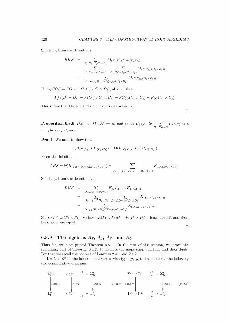
126 CHAPTER 6. THE CONSTRUCTION OF HOPF ALGEBRAS
Similarly, from the definitions,
RHS =∑
F1,F2: FiCi=Di
M(F1,D1) ∗M(F2,D2)
=∑
F1,F2: FiCi=Di
∑F : GF=jG(F1×F2)
M(F,FjG(D1×D2))
=∑
F : GFjG(C1×C2)=jG(D1×D2)
M(F,FjG(D1×D2)).
Using FGF = FG and G ≤ jG(C1 × C2), observe that
FjG(D1 ×D2) = FGFjG(C1 × C2) = FGjG(C1 × C2) = FjG(C1 × C2).
This shows that the left and right hand sides are equal.�
Proposition 6.8.6 The map Θ : N → R that sends H(P,C) to∑
D: PD=C
K(D,C) is a
morphism of algebras.
Proof We need to show that
Θ(H(P1,C1) ∗H(P2,C2)) = Θ(H(P1,C1)) ∗Θ(H(P2,C2)).
From the definitions,
LHS = Θ(H(jG(P1×P2),jG(C1×C2))) =∑
D: jG(P1×P2)D=jG(C1×C2)
K(D,jG(C1×C2)).
Similarly, from the definitions,
RHS =∑
D1,D2: PiDi=Ci
K(D1,C1) ∗K(D2,C2)
=∑
D1,D2: PiDi=Ci
∑D: GD=jG(D1×D2)
K(D,jG(C1×C2))
=∑
D: jG(P1×P2)GD=jG(C1×C2)
K(D,jG(C1×C2)).
Since G ≤ jG(P1 × P2), we have jG(P1 × P2)G = jG(P1 × P2). Hence the left and righthand sides are equal.
�
6.8.9 The algebras AZ, AL, AZ∗ and AL∗
Thus far, we have proved Theorem 6.8.1. In the rest of this section, we prove theremaining part of Theorem 6.1.2. It involves the maps supp and lune and their duals.For that we recall the content of Lemmas 2.4.1 and 2.4.2.
Let G ∈ Σn be the fundamental vertex with type (g1, g2). Then one has the followingtwo commutative diagrams.
ΣnG� � //
suppnG
����
ΣnG· // //
suppn
����
ΣnG
suppnG
����LnG
� � // LnG·
// // LnG
Σg1 × Σg2
suppg1 × suppg2
����
jG
∼=// ΣnG
suppnG
����Lg1 × Lg2
jG
∼= // LnG
(6.35)

6.8. CONSTRUCTION OF ALGEBRAS 127
whereLnG = {X ∈ Ln | suppn(G) ≤ X}
is the poset of flats of ΣnG, and suppnG, suppg1 and suppg2 are the support maps of ΣnG,Σg1 and Σg2 respectively. The map G· : Σn → ΣnG sends F to GF . One also has thesame two diagrams above with Σ and L replaced by Q and Z respectively, and the mapsupp replaced by the map lune.
Definition 6.8.7 Define a product on AL∗ and AZ∗ by
mX1∗mX2
=∑
X: G·X=jG(X1×X2)
mX ,
mL1∗mL2
=∑
L: G·L=jG(L1×L2), G∈zone(L)
mL.
The set zone(L) is discussed in Section 2.3.4. It also made an appearance in the coproductformula for AZ , see Definition 6.5.8. One way to justify its presence is by the conditionG ∈ reg(F,D) which occurs in the second product formula for Q, see the remark afterDefinition 6.8.3.
We say that a X (resp. L) as above is a quasi-shuffle of the flats X1 and X2 (resp.lunes L1 and L2).
Definition 6.8.8 Define a product on AL and AZ by
hX1∗ hX2
= hjG(X1×X2),
hL1∗ hL2
= hjG(L1×L2).
We say that jG(X1×X2) (resp. jG(L1×L2)) is the join of the flats X1 and X2 (resp.lunes L1 and L2).
Remark For the example of type An−1, one can make explicit the maps G· in thediagram (6.35) above, as also the join maps jG : Lg1 × Lg2 → LnG and jG : Zg1 × Zg2 →ZnG. It is then easy to check that the above formulas reduce to the definitions of thecorresponding algebras in Section 6.2.
Proposition 6.8.7 Let {Σn} be a family of LRBs, and let P, M, Q and N be thealgebras as given in Definitions 6.8.1-6.8.4.
(1) The injective maps supp∗ : AL∗ → P that sends mX to∑
F : suppF=X
MF and lune∗ :
AZ∗ → Q that sends mL to∑
(F,D): lune(F,D)=L
M(F,D) are maps of algebras.
(2) The surjective maps supp :M։ AL that sends HP to hsuppP and lune : N ։ AZ
that sends H(P,C) to hlune(P,C) are maps of algebras.
Proof We only give the proof for the supp and supp∗ maps.
(1) The following computation shows that the map supp∗ : AL∗ → P is a morphism ofalgebras. The term supp∗(mX1
) ∗ supp∗(mX2) equals
=∑
Fi: suppFi=Xi
MF1∗MF2
=∑
Fi: suppFi=Xi
∑F : GF=jG(F1×F2)
MF
=∑
F : supp(GF )=jG(X1×X2)
MF (Diagram (6.35))
=∑
F : supp(G)∨supp(F )=jG(X1×X2)
MF
=∑
X: G·X=jG(X1×X2)
∑F : suppF=X
mF ,

128 CHAPTER 6. THE CONSTRUCTION OF HOPF ALGEBRAS
which equals supp∗(mX1∗mX2
).
(2) It follows from diagram (6.35) that
supp(jG(P1 × P2)) = jG(supp(P1)× supp(P2)).
This proves that the map supp :M։ AL is a morphism of algebras.�

Chapter 7
The Hopf algebra of pairs of
permutations
7.1 Introduction
In this chapter, we study in detail the Hopf algebra SΠ indexed by pairs of permutationsthat was introduced in Chapter 6.
7.1.1 The basic setup
We recall some notation from Chapter 1, see Section 1.4 in particular. More backgroundmaterial for this chapter can be found in Section 5.4.
Let Sn be the symmetric group on n letters and Σn be its Coxeter complex. The groupSn is generated by S = {s1, . . . , sn−1}, where si is the transposition that interchanges iand i+ 1. Identify Q
n, the poset of compositions of n under refinement, with the poset
of subsets of S under inclusion in the usual way. Let Cn be the set of chambers in Σn.Since Sn acts simply transitively on Cn, one can identify
Cn ←→ Sn (7.1)
after fixing a fundamental chamber Cn0 ∈ Cn. We use the standard notation that wCn0 is
the chamber that corresponds to w ∈ Sn.Let d : Cn×Cn → Sn be the distance map, and type : Σn → Q
nmap a face to its type.
Note that d(Cn0 , wCn0 ) = w. We sometimes drop the superscript n to avoid overloading
the notation. We write F for the opposite of the face F ∈ Σn. The letters C, D and E
always stand for chambers.
7.1.2 The main result
Standard material
In [61], Malvenuto introduced the Hopf algebra
SΛ =∑
n≥0
K(Sn)∗,
indexed by permutations, and related it to the Hopf algebra of quasi-symmetric functionsQΛ via the descent map. Recall that:
Theorem 7.1.1 SΛ is a self-dual free and cofree graded Hopf algebra.
129

130 CHAPTER 7. THE HOPF ALGEBRA OF PAIRS OF PERMUTATIONS
Table 7.1: Hopf algebras and their indexing sets and bases.
Name Vector space Bases Name Dual space Dual bases
RΠ K(Cn × Cn) R,H,K SΠ K(Cn × Cn)∗ S,M,F
RΛ KSn H,K SΛ K(Sn)∗ M,F
The self-duality appears in Malvenuto’s thesis [61, Section 5.2] and Malvenuto andReutenauer [62, Theorem 3.3] and the freeness was established by Poirier and Reutenauer [78].For ideas related to the Hopf algebra SΛ, see Reutenauer [82], Patras and Reutenauer [73],Loday and Ronco [56, 57], Duchamp, Hivert and Thibon [26, 27], Foissy [30] and Aguiarand Sottile [4, 3, 5].
New material
In Chapter 5, we initiated a systematic study of the descent theory of Coxeter groups.This pointed us to the fact that one should be able to realize the Hopf algebra SΛ as aquotient of a bigger Hopf algebra indexed by pairs of permutations. This goal was realizedin Chapter 6, where we constructed many new Hopf algebras following this philosophy.Among them was the Hopf algebra
SΠ = ⊕n≥0
K(Cn × Cn)∗, (7.2)
indexed by pairs of permutations. The definitions of the Hopf algebras SΠ and SΛ arerecalled in Section 7.2.
The goal of this chapter is to study in detail the Hopf algebra SΠ. Using the quotientmap SΠ ։ SΛ, one can then quickly derive some of the results obtained in [4] for SΛ.The main result of this chapter is:
Theorem 7.1.2 SΠ is a free and cofree graded Hopf algebra.
Note that we do not claim SΠ to be self-dual. The proof of Theorem 7.1.2 is a conse-quence of Theorems 7.4.3 and 7.5.4 that we establish in this chapter. In Sections 7.1.3-7.1.5 below, we recall relevant ideas from Chapters 5 and 6. In Section 7.1.6, we providean outline of the proof of Theorem 7.1.2, and explain the organization of the rest of thechapter.
7.1.3 The Hopf algebras RΠ and RΛ
For book-keeping purposes, we introduce two more Hopf algebras RΠ and RΛ, whichare isomorphic copies of SΠ and SΛ respectively, see Table 7.1. The nth graded pieceof each Hopf algebra is indicated in the vector space column, see Equation (7.2) in thisregard. For each Hopf algebra, we consider a number of useful bases. They are relatedto one another via certain partial orders on Cn × Cn and Sn. This theory was developedin Chapter 5 for any Coxeter group. We recall the main definitions in Sections 7.1.4and 7.1.5 below.
The precise relation among the above four Hopf algebras is given by the followingspecial case of Theorem 6.1.4.

7.1. INTRODUCTION 131
Proposition 7.1.1 The following is a commutative diagram of graded Hopf algebras.
RΠ
d
����
∼=
s // SΠ
d
����RΛ
∼=s
// SΛ
where the switch map s : RΠ→ SΠ sends K(D,C) to F(C,D), and s : RΛ→ SΛ sends Kw
to Fw−1 . The distance map d is given by
A(C,D) 7→ Ad(C,D)
for A = F,M,H and K. On the S basis, one has
S(C,D) 7→
Md(C,D) if D = C0,
0 otherwise.
Proof The commutativity of the diagram follows from the definitions of the maps. TheHopf algebras RΠ and RΛ are defined from the Hopf algebras SΠ and SΛ respectively,using the isomorphism s. So the content of the proposition is that the distance mapd : SΠ→ SΛ is a map of Hopf algebras. This is an easy check.
�
Remark It follows directly from the definitions in the F and K basis that RΛ ∼= SΛ∗
as Hopf algebras with Kw = F ∗w.
7.1.4 Three partial orders on Cn × Cn
We recall some definitions and facts from Section 5.2.4 and Section 1.3.5.
Definition 7.1.1 Let ≤ be the weak left Bruhat order on Sn. Using the identificationin (7.1), define a partial order ≤b on the set Cn as follows.
uCn0 ≤b vCn0 in Cn ⇐⇒ u ≤ v in Sn.
This occurs precisely if there is a minimum gallery
Cn0 − vu−1Cn0 − vC
n0 .
The subscript “b” stands for Bruhat. Note that this partial order depends on the choiceof the fundamental chamber Cn0 in Cn.
Similarly, we write ≤rb for the partial order on Cn defined using the weak right Bruhatorder on Sn. The only purpose of the partial order ≤rb is to allow us to make a commentabout the product of SΛ, see Definition 7.2.13.
Definition 7.1.2 We define three partial orders on Cn × Cn.
(C1, D1) ≤ (C2, D2) ⇐⇒ D1 = D2 = D and C2 − C1 −D.
⇐⇒ D1 = D2 = D and d(C1, D1) ≤ d(C2, D2).
(C1, D1) ≤′ (C2, D2) ⇐⇒ D1 ≤b D2 and d(C1, D1) = d(C2, D2).
(C1, D1) � (C2, D2) ⇐⇒ ∃E ∋ (C1, D1) ≤ (E,D1) and (E,D1) ≤′ (C2, D2).
Note that in the definition of�, only one E can satisfy the required condition; namely theone that satisfies d(E,D1) = d(C2, D2). Unlike ≤, the partial orders ≤′ and � dependon the choice of the fundamental chamber Cn0 .

132 CHAPTER 7. THE HOPF ALGEBRA OF PAIRS OF PERMUTATIONS
7.1.5 The different bases of SΠ and SΛ
We recall some definitions from Section 5.6.1 and Section 5.7.1. The M basis of SΛ wasintroduced in [4]. It is related to the F basis by the weak left Bruhat order ≤ on Sn asfollows.
Fv =∑
u: v≤u
Mu.
Let RΛ be the graded dual of SΛ as a Hopf algebra, and H and K be the bases dual toM and F respectively. Then
Hu =∑
v: v≤u
Kv.
In the literature, it is RΛ rather than SΛ that is sometimes referred to as the Malvenuto-Reutenauer Hopf algebra.
Similarly, using the partial orders in Definition 7.1.2, we define the S, M and F basesof SΠ. They are related by
F(E,D) =∑
C: (E,D)≤(C,D)
M(C,D), M(C′,D′) =∑
(C′,D′)≤′(C,D)
S(C,D). (7.3)
Observe from the above formulas that the F basis is related to the S basis via the partialorder � as follows.
F(C′,D′) =∑
(C′,D′)�(C,D)
S(C,D).
Let RΠ be the graded dual of SΠ as a vector space. Then the R, H and K dual basesare related by
H(E,C) =∑
D: (D,C)≤(E,C)
K(D,C), R(D′,C′) =∑
(D,C)≤′(D′,C′)
H(D,C). (7.4)
We draw the reader’s attention to the fact that RΠ is not defined as the graded Hopfalgebra dual of SΠ.
7.1.6 The proof method and the organization of the chapter
Standard material
We first review the method for proving Theorem 7.1.1. It follows directly from thedefinitions in the F and K basis that RΛ ∼= SΛ∗ as Hopf algebras with Kw = F ∗
w. This
implies that SΛ is a self-dual Hopf algebra with SΛ∗∼=−→ SΛ given by F ∗
w 7→ Fw−1 . Asmentioned before, freeness and cofreeness of SΛ follows from results of Malvenuto, Poirier,and Reutenauer [61, 62, 78]. Other proofs are given in [27, 4]. Explicit expressions forthe product and coproduct in the M basis are given in [4].
New material
In order to prove Theorem 7.1.2, we apply similar ideas. However it is not true thatRΠ ∼= SΠ∗ as Hopf algebras with K(D,C) = F ∗
(D,C). So one cannot conclude that SΠ isself-dual. This doubles our work and one has to prove the freeness and cofreeness of SΠseparately.
In Section 7.2, we recall the definition of the Hopf algebra SΠ in the F basis as givenin Chapter 6. In Section 7.3, we compute the coproduct and product in the M basisof SΠ. The formulas for SΛ in the M basis obtained in [4] follow directly from these.However, unlike for SΛ, one cannot conclude cofreeness of SΠ from the coproduct formulain the M basis, since it produces some unwanted terms.

7.2. THE HOPF ALGEBRA SΠ 133
This flaw is rectified by replacing theM basis by the S basis. The coproduct computa-tion in the S basis in Section 7.4 produces exactly the terms that we want. In particular,it shows that SΠ is cofree, thus proving one part of Theorem 7.1.2. For completeness,we also write down the product in the S basis.
In Section 7.5, we compute the coproduct and product in the H basis of RΠ. Thefreeness of RΠ, and hence SΠ, follows from the product formula in the H basis of RΠ,proving the second part of Theorem 7.1.2.
Open Question For completeness, one would also like to compute the formulas inthe R basis of RΠ and formulas for the antipode in the various bases. These are openproblems at the moment.
Remark There is a way to recover the “self-duality” of SΠ by viewing it as a Hopfmonoid in a certain category of species. One can also derive the antipode formulas forSΛ obtained in [4] by this approach. These ideas will be explained in a future work.
7.2 The Hopf algebra SΠ
In this section, we recall the definition of the Hopf algebra SΠ in the F basis in both com-binatorial and geometric terms as given in Chapter 6. Then we recall the combinatorialdefinition of SΛ in the F basis and give a new geometric definition.
7.2.1 Preliminary definitions
We first give a few preliminary definitions, some of which were written in Section 6.2.3.
Definition 7.2.1 A set composition is an ordered set partition. For example, 6|34|125is a composition of [6].
Definition 7.2.2 There is a unique order preserving map from any n-set N of integersto the standard n-set [n]. Using this map, one can standardize compositions of N tocompositions of [n]. For example,
st(8|36|59) = 4|13|25.
Definition 7.2.3 The join of a composition F1 of [g1] and a composition F2 of [g2] is acomposition j(F1 × F2) of [g1 + g2] obtained by shifting up the indices of F2 by g1 andthen placing it after F1. For example,
j(31|2× 23|14|5) = 31|2|56|47|8.
We also define j(F1 × F2) to be the composition of [g1 + g2] obtained by shifting up theindices of F2 by g1 and then placing it before F1. For example,
j(31|2× 23|14|5) = 56|47|8|31|2.
Further, we define j′(F1 × F2) to be the composition of [g1 + g2] obtained by shifting upthe indices of F1 by g2 and then placing it before F2. For example,
j′(31|2× 23|14|5) = 86|7|23|14|5.
Further, we define j′′(F1×F2) to be the composition of [g1 + g2] obtained by shifting upthe indices of F1 by g2 and then placing it after F2. For example,
j′′(31|2× 23|14|5) = 23|14|5|86|7.

134 CHAPTER 7. THE HOPF ALGEBRA OF PAIRS OF PERMUTATIONS
Definition 7.2.4 A shuffle of set compositions F1 and F2 is a shuffle of the componentsof F1 and F2. For example,
5|bc|af |21|34|deg|6 is a shuffle of 5|21|34|6 and bc|af |deg.
Definition 7.2.5 A quasi-shuffle of set compositions F1 and F2 is a shuffle of the com-ponents of F1 and F2, where in addition we are allowed to substitute a disjoint set ofpairs of components (F i1 , F
j2 ) for F i1∪F
j2 , if they are adjacent in the shuffle. For example,
5bc|af |21|34deg|6 is a quasi-shuffle of 5|21|34|6 and bc|af |deg.
The above definitions of a shuffle and quasi-shuffle are not fully precise since oneneeds to ensure that the shuffled sets are disjoint, see Section 6.2.3 for more details.
7.2.2 Combinatorial definition
The Coxeter complex Σn can be identified with the poset of set compositions underrefinement. This allows us to define SΠ in combinatorial terms, without any referenceto Coxeter complexes, as below. Let C = C1|C2| . . . |Cn and D = D1|D2| . . . |Dn be twopermutations.
Definition 7.2.6 The coproduct on SΠ is given by
∆(F(C,D)) =
n∑
i=0
Fst(C1|···|Ci,D1|···|Di) ⊗ Fst(Ci+1|···|Cn,Di+1|···|Dn),
where C1, . . . , Ci are the letters in the set {D1, . . . , Di} and Ci+1, . . . , Cn are the lettersin the set {Di+1, . . . , Dn} written in the order in which they appear in C1| · · · |Cn. Forexample,
∆(F2|3|1|4,4|1|2|3) = 1⊗ F2|3|1|4,4|1|2|3 + F1,1 ⊗ F2|3|1,1|2|3 + F1|2,2|1 ⊗ F1|2,1|2+
F2|1|3,3|1|2 ⊗ F1,1 + F2|3|1|4,4|1|2|3 ⊗ 1.
Definition 7.2.7 The product on SΠ is given by
F(C1,D1) ∗ F(C2,D2) =∑
D: D a shuffle of D1 and D2
F(j(C1×C2),D).
The term j(C1 ×C2) refers to the join of C1 and C2 given in Definition 7.2.3. If D1 andD2 are compositions of [g1] and [g2] respectively then the understanding is that we shiftup the indices of D2 by g1 and then shuffle. For example,
F(2|1,1|2) ∗ F(1|2,2|1) = F(2|1|3|4,1|2|4|3) + F(2|1|3|4,1|4|2|3) + F(2|1|3|4,1|4|3|2)+
F(2|1|3|4,4|1|2|3) + F(2|1|3|4,4|1|3|2) + F(2|1|3|4,4|3|1|2).
Note that the first coordinate is the same in each term in the right hand side.
Proposition 7.2.1 With the coproduct and product as above, SΠ is a Hopf algebra.
We leave the proof to the reader.

7.2. THE HOPF ALGEBRA SΠ 135
7.2.3 The break and join operations
We recall the construction of the break and join operations for the family {Σn}, as nvaries (Sections 6.3.3 and 6.6.3). Let
ΣnK = {F ∈ Σn | K ≤ F}
be the star region of the face K. It can be identified with link(K), which is a Coxetercomplex in its own right.
For a vertex K ∈ Σn of type (k1, k2), we have an isomorphism
ΣnK∼=−→ Σk1 ∗ Σk2 ,
where Σk1 ∗ Σk2 is the join of Σk1 and Σk2 . This is because deleting a vertex in theCoxeter diagram of type A results in two smaller diagrams both of type A. Howeverthere is a choice involved in this isomorphism because of the action of the symmetricgroups Sk1 and Sk2 . We fix an isomorphism
bK : ΣnK∼=−→ Σk1 × Σk2 , by demanding that KCn0 7→ Ck10 × C
k20 ,
where KCn0 is the projection of Cn0 on K, see Figure 1.2. Recall from Section 1.3.1 thatthese projection maps define a semigroup structure on Σn. For F,G ∈ Σn, we denote theproduct by FG, and call it the projection of G on F .
Similarly, one defines an isomorphism
jG : Σg1 × Σg2∼=−→ ΣnG, by demanding that C
g10 × C
g20 7→ Cn0 ,
where G ∈ Cn0 is the fundamental vertex of type (g1, g2).The letters b and j stand for “break” and “join” respectively. In our arguments, we
often refer to the compatibility of galleries with the maps bK and jG. This is same asthe compatibility of galleries with joins (Section 1.3.7).
7.2.4 Geometric definition
The Hopf algebra SΠ can be described geometrically using the semigroup structure ofΣn and the maps bK and jG as below.
Definition 7.2.8 The coproduct on SΠ is given by
∆(F(C,D)) = 1⊗ F(C,D) + F(C,D) ⊗ 1 + ∆+(F(C,D)), where
∆+(F(C,D)) =∑
K: rankK=1, K≤D
F(C1,D1) ⊗ F(C2,D2),
where for bK : ΣnK → Σk1 × Σk2 , we have bK(D) = D1 ×D2 and bK(KC) = C1 × C2.
Definition 7.2.9 The product on SΠ is given by
F(C1,D1) ∗ F(C2,D2) =∑
D: GD=jG(D1×D2)
F(jG(C1×C2),D).
The vertex G ∈ Σn is fixed in the above sum. It is the vertex of Cn0 of type (g1, g2),where Ci ∈ Σgi .
Equivalently, the sum ranges over the chambers D in reg(G,D′), which is the lunarregion of G and D′ = jG(D1 ×D2), as shown in Figure 7.1. A more concrete example isgiven in Figure 7.2.
For a discussion of lunes, see Section 2.3 and the references therein. The maps bK ,jG and the semigroup structure of Σn can be described combinatorially. Using them,one can recover the combinatorial definitions of the product and coproduct for SΠ givenearlier. This is explained in some detail in Chapter 6.

136 CHAPTER 7. THE HOPF ALGEBRA OF PAIRS OF PERMUTATIONS
G D′
D
Figure 7.1: A chamber D in reg(G,D′), the lunar region of G and D′.
7.2.5 The Hopf algebra SΛ
In this subsection, we use chambers rather than permutations to index SΛ. We first recallthe combinatorial definition of SΛ in the F basis.
Definition 7.2.10 The coproduct on SΛ is given by
∆(FD) =
n∑
i=0
Fst(D1|···|Di) ⊗ Fst(Di+1|···|Dn).
Definition 7.2.11 The product on SΛ is given by
FD1∗ FD2
=∑
D: D a shuffle of D1 and D2
FD.
In geometric terms, the definitions are as follows.
Definition 7.2.12 The coproduct on SΛ is given by
∆(FD) = 1⊗ FD + FD ⊗ 1 +∑
K: rankK=1, K≤D
FD1⊗ FD2
,
where for bK : ΣnK → Σk1 × Σk2 , we have bK(D) = D1 ×D2.
Definition 7.2.13 The product on SΛ is given by
FD1∗ FD2
=∑
D: GD=jG(D1×D2)
FD.
The vertex G ∈ Σn is the vertex of Cn0 of type (g1, g2), where Ci ∈ Σgi .By definition, the sum ranges over the chambers D in reg(G,D′), which is the lunar
region of G and D′ = jG(D1 ×D2). Equivalently, the sum ranges over D such that
D′ ≤rb D ≤rb GD′
in the weak right Bruhat order ≤rb on Cn given in Definition 7.1.1. This relation of theproduct in SΛ to the weak right Bruhat order appears in Loday and Ronco [57]. Fromthe remark after Lemma 5.3.2, it is clear that one can also define the product in SΛ bysumming over T -shuffles where T = typeG.
As an example,
F2|1 ∗ F1|2 = F2|1|3|4 + F2|3|1|4 + F2|3|4|1 + F3|2|1|4 + F3|2|4|1 + F3|4|2|1.
The chambers that occur in the right hand side are precisely those in reg(12|34, 2|1|3|4),which is the shaded region in Figure 7.2.
From the discussion in this section, one also observes that:
Proposition 7.2.2 The map SΠ → SΛ that sends F(C,D) → FD is a map of Hopfalgebras.

7.3. THE HOPF ALGEBRA SΠ IN THE M BASIS 137
����������������������������������������������������������������������������������������������������������������������������������
����������������������������������������������������������������������������������������������������������������������������������
������
����
2413 2431
2341
23142134
2143
12431234
1324 3124
3214
3412
3421
314213421432
1423
3241
1−2
2−4
2−3
3−4
1−4
1−3
Figure 7.2: A lunar region in the Coxeter complex Σ4.
7.3 The Hopf algebra SΠ in the M basis
In this section, we write down formulas for the coproduct and product in the M basisof SΠ. We also show how they can be used to deduce the corresponding formulas forSΛ obtained in [4]. The global descent maps GDes : Cn × Cn → Σn and gdes : Sn → S
appear in the computations. For more details on these maps, see Sections 5.2-5.4.
7.3.1 A preliminary result
In order to compare the coproducts in the F and M basis, we need to relate the partialorder ≤ in Σn to the same partial order restricted to a star region ΣnK . The precisefact which is needed is stated below and it is valid for the poset of faces of any centralhyperplane arrangement.
Fact 7.3.1 Let K ≤ C,D. Then
(E,D) ≤ (C,D) ⇐⇒ (KE,D) ≤ (KC,D).
Proof The reader may refer to Figure 7.3. The assumption K ≤ C,D implies thatKC and C are opposite chambers in star(K). The lemma follows from the followingequivalences.
(E,D) ≤ (C,D) ⇐⇒ C − E −D (Definition 7.1.1)
⇐⇒ C − E −KE −D (Gate property)
⇐⇒ C −KE −D − C
⇐⇒ C −KC −KE −D − C (Gate property)
⇐⇒ KC −KE −D
⇐⇒ (KE,D) ≤ (KC,D) (Definition 7.1.1).
For the backward implication of the third equivalence, note that we always have thegallery C − E − C. By the gate property, we then get C − E −KE − C, which alongwith KE−D−C gives the gallery C −E−KE−D. For the second to last equivalence,we use the observation made at the beginning of the proof.
�

138 CHAPTER 7. THE HOPF ALGEBRA OF PAIRS OF PERMUTATIONS
7.3.2 Coproduct in the M basis
Theorem 7.3.1 The coproduct on SΠ is given by
∆(M(C,D)) = 1⊗M(C,D) +M(C,D) ⊗ 1 + ∆+(M(C,D)), where
∆+(M(C,D)) =∑
K: rankK=1, K≤D, K≤C
M(C1,D1) ⊗M(C2,D2),
where for bK : ΣnK → Σk1 × Σk2 , we have bK(D) = D1 ×D2 and bK(KC) = C1 × C2.
Comparing with Definition 7.2.8, the coproduct in the M basis has fewer terms than inthe F basis due to the additional condition K ≤ C on K. Since GDes(C,D) = D ∩ C,one can equivalently write the condition on K as K ≤ GDes(C,D), rankK = 1.
Proof To prove the theorem, we start with the above formula and derive the coproductin the F basis. The chambers D and E are fixed in the computation and K is a vertexthat varies.
KK
D
E
KE
C = KC ′ C′ = KC C
Figure 7.3: The close relation between the star regions of K and K.
It is useful to keep Figure 7.3 in mind. The steps in the computation are as below.The justification for the main steps are provided after the computation.
∆+(F(E,D)) =∑
C: (E,D)≤(C,D)
∆+(M(C,D)) (Relation (7.3))
=∑
(K,C): rankK=1
K≤D, K≤C, (E,D)≤(C,D)
M(C1,D1) ⊗M(C2,D2)
(bK(D)=D1×D2
bK(KC)=C1×C2.
)
=∑
(K,C′): rankK=1K≤D, K≤C′, (KE,D)≤(C′,D)
M(C1,D1) ⊗M(C2,D2)
(bK(D)=D1×D2
bK(C′)=C1×C2.
)
=∑
(K,C1,C2): rankK=1K≤D, (Ei,Di)≤(Ci,Di)
M(C1,D1) ⊗M(C2,D2)
(bK(D)=D1×D2
bK(KE)=E1×E2.
)
=∑
K: rankK=1, K≤D
F(E1,D1) ⊗ F(E2,D2). (Relation (7.3))
For the third equality, given K, the chambers C and C′ determine each other by therelations C′ = KC and C = KC′, as indicated in Figure 7.3. The equivalence betweenthe conditions (E,D) ≤ (C,D) and (KE,D) ≤ (C′, D) in this situation is the content ofFact 7.3.1, which was proved above. We now recall that star regions are convex. Sincethe partial order ≤ is defined by a gallery condition, we have
(KE,D) ≤ (C′, D) in the complex Σn ⇐⇒ (KE,D) ≤ (C′, D) in the complex ΣnK .
Hence all the action is now happening in the smaller Coxeter complex ΣnK .

7.3. THE HOPF ALGEBRA SΠ IN THE M BASIS 139
For the fourth equality, given K, the chamber C′ and the pair (C1, C2) determineeach other because the map bK is an isomorphism. The equivalence of the conditions(KE,D) ≤ (C′, D) and (Ei, Di) ≤ (Ci, Di) is due to the compatibility of galleries withthe map bK .
�
Let C = C1|C2| . . . |Cn and D = D1|D2| . . . |Dn be two permutations. Recall thatDefinition 5.4.4 implies that
si ∈ type(GDes(C,D)) ⇐⇒ Dj appears after Dk in C for all j ≤ i and i+ 1 ≤ k.
If this happens then one says that the chamber D has a global descent of type si, orat position i, with respect to the chamber C. This fact can be used to derive thecombinatorial content of Theorem 7.3.1 given below. We omit the details, since they aresimilar to those involved in showing that Definitions 7.2.6 and 7.2.8 are equivalent.
Theorem 7.3.2 The coproduct on SΠ is given by ∆+(M(C,D)) =
∑
si: si∈type(GDes(C,D))
Mst(Cn−i+1|···|Cn,D1|···|Di) ⊗Mst(C1|···|Cn−i,Di+1|···|Dn).
As an example,
∆(M(2|1|3,1|3|2)) = 1⊗M(2|1|3,1|3|2) +M(2|1|3,1|3|2) ⊗ 1 +M(1|2,1|2) ⊗M(1,1).
Remark From the above theorem, one cannot conclude that SΠ is cofree. This isbecause, given M(C1,D1) and M(C2,D2), one cannot uniquely recover M(C,D). However,the M basis is much better than the F basis to study the coradical filtration of SΠ. Forexample, one sees directly that the elements in the set
{M(C,D) | GDes(C,D) = D ∩ C = ∅}
are primitive. The graded cardinalities of the above set are 1, 2, 18, etc. Direct handcomputation from the coproduct formula shows that the graded dimensions of the space ofprimitive elements are 1, 3, 29, etc. In the first two degrees, M(1,1), M(1|2,1|2), M(2|1,2|1),and M(1|2,2|1) −M(2|1,1|2) provide a basis for the primitive elements.
Theorem 7.3.3 [4, Theorem 3.1] Let w = w1| . . . |wn be a permutation. The coproducton SΛ is given by
∆(Mw) = 1⊗Mw +Mw ⊗ 1 +∑
si: si∈gdes(w)
Mst(w1|...|wi) ⊗Mst(wi+1|...|wn).
Proof Take C = Cn0 = 1|2| . . . |n and D = wCn0 in the previous theorem and thenproject down the formula to SΛ via the distance map. The result follows by noting thatd(Cn0 , uC
n0 ) = u and type(GDes(Cn0 , wC
n0 )) = gdes(w).
�
For si ∈ gdes(w), given w1 = st(w1| . . . |wi) and w2 = st(wi+1| . . . |wn), one canuniquely recover w as j′(w1 × w2), with j′ as in Definition 7.2.3. Hence, in contrastto the situation for SΠ, the formula in the M basis shows that SΛ is cofree. This isexplained in detail in the proof of [4, Theorem 6.1].

140 CHAPTER 7. THE HOPF ALGEBRA OF PAIRS OF PERMUTATIONS
7.3.3 Product in the M basis
Theorem 7.3.4 The product on SΠ is given by
M(C1,D1) ∗M(C2,D2) =∑
(C,D):M(i): GD=jG(D1×D2)M(ii): GC=jG(C1×C2)M(iii): C−GC−GD−D
M(C,D).
The vertex G ∈ Σn is as in Definition 7.2.9.
G
C
D
E
C ′ D′
GG
Figure 7.4: The term M(C,D) occurring in the product M(C1,D1) ∗M(C2,D2).
In Figure 7.4, we have used the notation C′ = jG(C1 ×C2) and D′ = jG(D1 ×D2). Thetwo lunar regions shown in the figure lie on a sphere and are supposed to meet at G, thevertex opposite to G. For simplicity, this is not shown in the figure, where there are twovertices labeled G.
Proof As in Theorem 7.3.1, to prove this theorem, we start with the above formulaand derive the product in the F basis. We use the following simple consequence of thegate property.
For G ≤ E, C −GC − E −GD −D ⇐⇒ C − E −D. (7.5)
Let M(1) denote the condition
(jG(E1 × E2), jG(D1 ×D2)) ≤ (jG(C1 × C2), jG(D1 ×D2)),
or equivalently, jG(C1 × C2)− jG(E1 × E2)− jG(D1 ×D2).The vertex G and the chambers E1, E2, D1 and D2 are fixed in the computation
below. For the simplicity of notation, we denote the conditions M(1), M(i), M(ii) andM(iii) simply as (1),(i),(ii) and (iii) respectively.
F(E1,D1) ∗ F(E2,D2) =∑
C1,C2:(1)
M(C1,D1) ∗M(C2,D2)
(Compatibility ofgalleries with themap jG.
)
=∑
C1,C2:(1)
∑C,D:
(i),(ii),(iii)
M(C,D) (Theorem 7.3.4)
=∑D:(i)
∑C:
(1),(ii),(iii)
M(C,D)
(Switching the order ofthe summations.
)
=∑D:(i)
∑C:
C−jG(E1×E2)−D
M(C,D) (7.5)
=∑D:(i)
F(jG(E1×E2),D). (Relation (7.3))
For the third equality, also note that C determines C1 and C2, since jG is an isomorphism.Hence we can get rid of them from the summation.
�

7.3. THE HOPF ALGEBRA SΠ IN THE M BASIS 141
The combinatorial content of the above statement is as below. Let (Ci, Di) ∈ Σgi fori = 1, 2 and let [g1 + 1, g1 + g2] = {g1 + 1, . . . , g1 + g2}.
Theorem 7.3.5 The product on SΠ is given by
M(C1,D1) ∗M(C2,D2) =∑
(C,D): —
M(C,D),
where — says that C (resp. D) is a shuffle of C1 and C2 (resp. D1 and D2) such thatif ∗1 ∈ [g1] and ∗2 ∈ [g1 + 1, g1 + g2] then ∗2 does not appear before ∗1 in both C and D.
As an example,
M(1|2,2|1) ∗M(1,1) = M(1|2|3,2|1|3) +M(1|3|2,2|1|3) +M(3|1|2,2|1|3)
+M(1|2|3,2|3|1) +M(1|3|2,2|3|1) +M(1|2|3,3|2|1).
Theorem 7.3.6 [4, Theorem 4.1] Let u ∈ Sg1 , v ∈ Sg2 with g1 + g2 = n. Also letG = 1 . . . g1|g1 + 1 . . . n be the fundamental vertex in Σn of type (g1, g2). The product onSΛ is given by
Mu ∗Mv =∑
w
|S0w(u × v)| Mw,
where
S0w(u× v) =
(C,D) ∈ Cn × Cn, d(C,D) = w,GD = Cn0
∣∣∣∣C −GC −GD −D
GC = (u−1 × v−1)Cn0 .
There are two more sets S+w (u × v) and S−
w (u × v), more combinatorial in nature, withthe same cardinality as S0
w(u × v). This is explained in detail in Lemma 5.3.2. Thedescription in [4] for the above product is given using the set S+
w (u× v).
Proof Specialize Theorem 7.3.4 to the chambers C1 = u−1Cg10 , C2 = v−1C
g20 , D1 = C
g10
and D2 = Cg20 . Then note that d(C1, D1) = u and d(C2, D2) = v. Now the result follows
by projecting to SΛ via the distance map and noting that jG(Cg10 × Cg20 ) = Cn0 .
�
7.3.4 The switch map on the M basis
We note a striking feature of the formulas in the M basis of SΠ. In contrast to theformulas in the F basis, the two coordinates of C × C now play a symmetric role. Weformulate this precisely as a corollary to Theorems 7.3.1 and 7.3.4.
Corollary 7.3.1 The map SΠ→ SΠ that sends M(C,D) to M(D,C) is a map of algebrasand a map of anti-coalgebras.
Proof The algebra part is clear. The coalgebra part follows from the following fact.
bK(D) = D1 ×D2, bK(KD) = D′1 ×D
′2 =⇒ D′
1 = D2, D′2 = D1.
In other words, shifting from K to K has the effect of interchanging the factors.�
Applying the map SΠ ։ SΛ of Hopf algebras that sends M(C,D) to Md(C,D), oneobtains:
Corollary 7.3.2 The map SΛ → SΛ that sends Mw to Mw−1 is a map of algebras anda map of anti-coalgebras.

142 CHAPTER 7. THE HOPF ALGEBRA OF PAIRS OF PERMUTATIONS
7.4 The Hopf algebra SΠ in the S basis
In this section, we write down formulas for the coproduct and product in the S basis ofSΠ. From the coproduct formula, we conclude that SΠ is a cofree coalgebra, thus provingone half of Theorem 7.1.2.
7.4.1 Two preliminary results
In order to compare the coproducts in the M and S basis, we need to relate the partialorder ≤′ in Σn to the same partial order restricted to a star region ΣnK′ . In particular, weneed to undertake such a study for the distance map d and the partial order ≤b, whichare a part of ≤′. The crucial facts about d and ≤b which are needed are stated below.They are valid for any Coxeter complex Σ. A special case of the second fact was provedin Chapter 5, see Proposition 5.3.7.
Fact 7.4.1 Let K and K ′ be faces of Σ of the same type. Also let C, D, C′ and D′ bechambers with K ≤ D,C and K ′ ≤ D′, C′. Then
d(C,D) = d(C′, D′) ⇐⇒ d(KC,D) = d(K ′C′, D′).
Proof The reader may refer to Figure 7.6.
For the forward implication, let w ∈ W be such that wC = C′ and wD = D′. Thensince the action of W on Σ is type-preserving, we get wK = K ′. This implies thatw(KC) = w(K ′C′), which proves the right hand side.
For the backward implication, let w ∈ W be such that w(KC) = K ′C′ and wD = D′.Then since the action of W on Σ is type-preserving, we get wK = K ′, which implieswK = K ′. Now K ≤ C and K ′ ≤ C′ implies that C = K(KC) and C′ = K ′(K ′C).Hence we obtain wC = C′, which proves the left hand side.
Fact 7.4.2 Let C0 be the chosen fundamental chamber in Σ. Also let K and K ′ be facesof Σ of the same type, with K ≤ C0. Then using the type-preserving action of W on Σ,we have an isomorphism
ΣK∼=−→ ΣK′ ,
sending KC0 7→ K ′C0, or equivalently, KC0 7→ K ′C0. Further, let
D ∈ ΣK ←→ D′′ ∈ ΣK′
correspond to each other under the above isomorphism. In other words,
d(KC0, D) = d(K ′C0, D′′) or equivalently, d(D,C0) = d(D′′,K ′C0). (7.6)
Let K ′ ≤ D′. Then
D′ ≤b D in the complex (Σ, C0) ⇐⇒ D′ ≤b D′′ in the complex (ΣK′ ,K ′C0).
We recall that the partial order ≤b depends on the choice of a fundamental chamber.This should clarify our use of the notation (Σ, C0) and (ΣK′ ,K ′C0).
As a special case, we obtain
D′′ ≤b D, and in particular, K ′C0 ≤b KC0.
The last conclusion was the content of Proposition 5.3.7; its alternative proof is beinggeneralized here.

7.4. THE HOPF ALGEBRA SΠ IN THE S BASIS 143PSfrag
KK ′
KC0
D
C0
D′
D′′
C0K ′C0 K ′C0
Figure 7.5: A comparison of two star regions.
Proof To get an idea of what is going on, the reader may refer to Figure 7.5. It showstwo bold dots, which are the faces K and K ′ of the same type. The hexagonal regionsgive a schematic picture of their star regions.
In order to use the definition of≤b, we first need to name chambers by group elements.Accordingly, letD = wC0, D
′ = w′C0, andD′′ = w′′C0. Then observe that w(w′)−1D′ =D and hence w(w′)−1K ′ = K. The fact now follows from the following sequence ofequivalences.
D′ ≤b D in (Σ, C0) ⇐⇒ C0 − w(w′)−1C0 −D (Definition 7.1.1)
⇐⇒ KC0 −K(w(w′)−1C0)−D (Fact 7.3.1)
⇐⇒ KC0 − w(w′)−1(K ′C0)−D (w(w′)−1K ′ = K)
⇐⇒ K ′C0 − w′′(w′)−1(K ′C0)−D′′
(Multiplyingby w′′w−1
)
⇐⇒ D′ ≤b D′′ in (ΣK′ ,K ′C0) (Definition 7.1.1).
We made use of the hypothesis K ≤ C0 in the second equivalence. In the fourth equiva-lence, we used Equation (7.6) to conclude that w′′(w′)−1 sends KC0 to K ′C0.
�
7.4.2 Coproduct in the S basis
Theorem 7.4.1 The coproduct on SΠ is given by
∆(S(C,D)) = 1⊗ S(C,D) + S(C,D) ⊗ 1 + ∆+(S(C,D)), where
∆+(S(C,D)) =∑
K: rankK=1, K≤D, K≤C,C0
S(C1,D1) ⊗ S(C2,D2),
where for bK : ΣnK → Σk1 × Σk2 , we have bK(D) = D1 ×D2 and bK(KC) = C1 × C2.
Comparing with Theorem 7.3.1, the coproduct in the S basis has fewer terms than inthe M basis due to the additional condition K ≤ C0 on K. In other words, the termGDes(C,D) is now replaced by C ∩D ∩ C0.
Proof To prove the theorem, we start with the above formula and derive the coproductin the M basis given by Theorem 7.3.1. The chambers C′ and D′ are fixed in thecomputation and K and K ′ are vertices that vary.
It is useful to bear Figure 7.6 in mind. The main steps, which are as below, are

144 CHAPTER 7. THE HOPF ALGEBRA OF PAIRS OF PERMUTATIONS
KK ′
K
KC
D
C
D′
C ′
D′′
C′′
C0
C0
K′C′
K ′C0
K ′
Figure 7.6: The relation between the coproducts in the M and S basis.
justified after the computation.
∆+(M(C′,D′)) =∑
(C,D): (C′,D′)≤′(C,D)
∆+(S(C,D)) (Relation (7.3))
=∑
(K,C,D): rankK=1
K≤D,C,C0, (C′,D′)≤′(C,D)
S(C1,D1) ⊗ S(C2,D2)
(bK(D)=D1×D2
bK(KC)=C1×C2.
)
=∑
(K′,C′′,D′′): rankK′=1
K′≤D′,C′, (K′C′,D′)≤′(C′′,D′′)
S(C1,D1) ⊗ S(C2,D2)
(bK′ (D′′)=D1×D2
bK′ (C′′)=C1×C2.
)
=∑
(K′,C1,C2,D1,D2): rankK′=1
K′≤D′,C′, (C′i,D
′i)≤
′(Ci,Di)
S(C1,D1) ⊗ S(C2,D2)
(bK′(D′)=D′
1×D′2
bK′ (K′C′)=C′1×C
′2.
)
=∑
K′: rankK′=1K′≤D′,C′
M(C′1,D
′1) ⊗M(C′
2,D′2)
(Relation (7.3))
We first point out that in the third step above, for lack of space, we have shortened theexpression
(K ′C′, D′) ≤′ (C′′, D′′) in the complex (ΣnK′ ,K ′C0),
to simply (K ′C′, D′) ≤′ (C′′, D′′). The heart of the proof lies in this step.The triplets (K,C,D) and (K ′, C′′, D′′), which index the summations on either side,
are related to each other by the relations
typeK = typeK ′, d(D,C0) = d(D′′,K ′C0) and d(KC,C0) = d(C′′,K ′C0),
as indicated in Figure 7.6. The reader should check that under these relations the tripletsdetermine each other. For example, given (K,C,D), one can define K ′ as the face of D′
of the same type as K, and so forth.The conditions (C′, D′) ≤′ (C,D) and (K ′C′, D′) ≤′ (C′′, D′′) are equivalent under
this correspondence. This follows from the following two facts.
d(C′, D′) = d(C,D) ⇐⇒ d(K ′C′, D′) = d(KC,D) (Fact 7.4.1)
⇐⇒ d(K ′C′, D′) = d(C′′, D′′) (Equation (1.5))
D′ ≤b D in (Σ, C0) ⇐⇒ D′ ≤b D′′ in (ΣK′ ,K ′C0) (Fact 7.4.2).
For the fourth equality, we require that
(K ′C′, D′) ≤′ (C′′, D′′) in (ΣK′ ,K ′C0) ⇐⇒ (C′i, D
′i) ≤
′ (Ci, Di) in (Σgi , Cgi
0 ),

7.4. THE HOPF ALGEBRA SΠ IN THE S BASIS 145
where we have bK′(D′′) = D1 × D2, bK′(C′′) = C1 × C2, bK′(D′) = D′1 × D′
2 andbK′(K ′C′) = C′
1 × C′2. This follows from the compatibility of the distance map and
galleries with joins. Also observe that bK′(K ′C0) = Cg10 × C
g20 . This is important since
the partial order ≤′ depends on the fundamental chamber.�
Theorem 7.4.2 The combinatorial formula for the coproduct in the S basis is given byTheorem 7.3.2 with the term GDes(C,D) replaced by C ∩D ∩ C0.
Also, from the definitions, one has
si ∈ type(C ∩D ∩ C0) ⇐⇒D has a global descent at position i andC has a global ascent at position n− i,
with the natural definition for a global ascent. As an example,
∆(S(1|3|2,2|3|1)) = 1⊗ S(1|3|2,2|3|1) + S(1|3|2,2|3|1) ⊗ 1 + S(2|1,1|2) ⊗ S(1,1).
The S basis does precisely what the M basis failed to do. Namely, it allows us to concludethat SΠ is cofree. This is because, given S(C1,D1) and S(C2,D2), one can uniquely recoverS(C,D), by the formula D = j′(D1 × D2) and C = j′′(C1 × C2), with j′ and j′′ as inDefinition 7.2.3. More precisely, let S0 = {1} and for k ≥ 1, let
Sk = {(C,D)∣∣ rank(C ∩D ∩ C0) = k − 1}.
Let SΠk be the vector subspace of SΠ spanned by {S(C,D) | (C,D) ∈ Sk}.
Theorem 7.4.3 With the above grading, SΠ is a cofree graded coalgebra. A basis forthe kth level of the coradical filtration of SΠ is
k∐
i=0
Sk.
In particular, a basis for the space of primitive elements is
{S(C,D) | C ∩D ∩ C0 = ∅}.
This follows directly from the definitions (Sections 3.1.1-3.1.2).
Remark We mention that Theorem 7.3.3 can also be deduced from Theorem 7.4.1 inthe same way as from Theorem 7.3.1.
7.4.3 Product in the S basis
Theorem 7.4.4 The product on SΠ is given by
S(C1,D1) ∗ S(C2,D2) =∑
(K,C,D):S(i): bK(KD)=D1×D2
S(ii): bK(KC)=C1×C2
S(iii): C−KC−KD−DS(iv): C0−KC0−KD−D
S(C,D).
The proof is left as an exercise to the reader. Unlike the product in the M basis givenby Theorem 7.3.4, we note that the above product depends on C0. The coefficient ofS(C,D) continues to be nonnegative but it can be greater than 1.
The combinatorial content of the above statement is as below. We recall that a vertexof type (g1, g2) is a two block composition of the set [g1+g2], with underlying composition(g1, g2). Now let (Ci, Di) ∈ Σgi for i = 1, 2.

146 CHAPTER 7. THE HOPF ALGEBRA OF PAIRS OF PERMUTATIONS
Theorem 7.4.5 The product on SΠ is given by
S(C1,D1) ∗ S(C2,D2) =∑
K=K1|K2:a vertex of type (g1,g2)
∑
(C,D): —
S(C,D),
where — says that C (resp. D) is a K-shuffle of C1 and C2 (resp. D1 and D2) such thatif ∗1 ∈ K1 and ∗2 ∈ K2 and ∗2 appears before ∗1 in D then ∗2 appears after ∗1 in bothC and C0.
The definition of a K-shuffle can be found in Definition 6.2.5, and its relation withconditions such as S(i) and S(ii) can be found in Equation (6.23). The condition aboveinvolving ∗1 and ∗2 is a translation of the gallery conditions S(iii) and S(iv). As anexample, the product S(1|2,2|1) ∗ S(1,1) equals
S(1|2|3,2|1|3) + S(1|3|2,2|1|3) + S(3|1|2,2|1|3) + S(1|2|3,2|3|1) + S(1|3|2,2|3|1) + S(1|2|3,3|2|1)
+S(1|3|2,3|1|2) + S(1|2|3,3|1|2) + S(2|1|3,3|1|2) + S(1|3|2,3|2|1) + S(1|2|3,3|2|1)
+S(2|3|1,3|2|1) + S(2|1|3,3|2|1) + S(1|2|3,3|2|1).
The three rows correspond to the vertices 12|3, 13|2 and 23|1 respectively, which are oftype (2, 1). Note that the term S(1|2|3,3|2|1) appears with coefficient 3.
Remark We mention that Theorem 7.3.6 can also be deduced from Theorem 7.4.4 inthe same way as from Theorem 7.3.4.
7.5 The Hopf algebra RΠ in the H basis
In this section, we write down formulas for the coproduct and product in the H basis ofRΠ. From the product formula, we conclude that RΠ, and hence SΠ, is a free gradedalgebra, thus proving the second half of Theorem 7.1.2. We also show how they can beused to deduce the formulas for the quotient RΛ, and observe that, as expected, they aredual to the formulas for SΛ deduced in Section 7.3.
The formulas in the K basis of RΠ are written in Definitions 6.5.6 and 6.8.6. They aresimply obtained from Definitions 7.2.8 and 7.2.9 by changing F to K and interchangingthe two coordinates. We use this in the computations.
7.5.1 Coproduct in the H basis
Theorem 7.5.1 The coproduct on RΠ is given by
∆(H(D,C)) = 1⊗H(D,C) +H(D,C) ⊗ 1 + ∆+(H(D,C)), where
∆+(H(D,C)) =∑
K: rankK=1, D−KD−KC−C
H(D1,C1) ⊗H(D2,C2),
where for bK : ΣnK → Σk1 × Σk2 , we have bK(KD) = D1 ×D2 and bK(KC) = C1 × C2.

7.5. THE HOPF ALGEBRA RΠ IN THE H BASIS 147
Proof This is a straightforward computation.
∆+(H(D,C)) =∑
E: D−E−C∆+(K(E,C)) (Relation (7.4))
=∑E:
D−E−C
∑K: rankK=1
K≤E
K(E1,C1) ⊗K(E2,C2)
(bK(E)=E1×E2
bK(KC)=C1×C2.
)
=∑
(K,E): rankK=1, K≤ED−KD−E−KC−C
K(E1,C1) ⊗K(E2,C2) (Gate property)
=∑
K: rankK=1D−KD−KC−C
∑E: K≤E
KD−E−KC
K(E1,C1) ⊗K(E2,C2)
=∑
K: rankK=1D−KD−KC−C
∑E1,E2:
Di−Ei−Ci
K(E1,C1) ⊗K(E2,C2)
(bK(KD)=D1×D2
bK(KC)=C1×C2.
)
=∑
K: rankK=1D−KD−KC−C
H(D1,C1) ⊗H(D2,C2). (Relation (7.4))
For the fifth equality, we used the compatibility of galleries with the map bK .
�
Theorem 7.5.2 The coproduct on RΛ is given by
∆(Hw) = 1⊗Hw +Hw ⊗ 1 +∑
u,v
|S−w (u× v)| Hu ⊗Hv.
To avoid repetition, we refer the reader to Section 5.3.6 for the definition of the setS−w (u× v). We note that this result is dual to that in Theorem 7.3.6, consistent with the
fact that RΛ ∼= SΛ∗ as Hopf algebras with Hw = M∗w. A proof is strictly not necessary;
but we give it to show how this result follows from the previous theorem.
Proof As in the proof of Theorem 7.3.3, we put D = Cn0 in the previous theorem, whichimplies that D1 = C
g10 and D2 = C
g20 , where typeK = (g1, g2). Now let C = wCn0 ,
C1 = uCg10 and C2 = vC
g20 , and apply the distance map. The coefficient of Hu ⊗Hv is
the number of vertices K of type (g1, g2) such that
C0 −K(wC0)− wC0 and bK(K(wC0)) = (u× v)C0.
Let σ be the (g1, g2)-shuffle which corresponds to K. Then the two conditions abovecorrespond to the conditions (i) and (ii) respectively in the set S−
w (u× v).
�
7.5.2 Product in the H basis
Theorem 7.5.3 The product on RΠ is given by
H(D1,C1) ∗H(D2,C2) = H(GjG(D1×D2),jG(C1×C2))
= H(j(D1×D2),j(C1×C2)). (Definition 7.2.3)
The vertex G ∈ Σn is as in Definition 7.2.9.

148 CHAPTER 7. THE HOPF ALGEBRA OF PAIRS OF PERMUTATIONS
Proof The second equality above follows from the first by using Definition 7.2.3. Wenow prove the first equality.
H(D1,C1) ∗H(D2,C2) =∑
E1,E2:Di−Ei−Ci
K(E1,C1) ⊗K(E2,C2)
=∑
E1,E2:Di−Ei−Ci
∑E:
GE=jG(E1×E2)
K(E,jG(C1×C2))
=∑E:
jG(D1×D2)−GE−jG(C1×C2)
K(E,jG(C1×C2))
=∑E:
GjG(D1×D2)−E−jG(C1×C2)
K(E,jG(C1×C2))
= H(GjG(D1×D2),jG(C1×C2)).
For the third equality, note that E determines E1, E2 because the map jG is an iso-morphism. We also used the compatibility of galleries with the map jG. For the fourthequality, we used the fact that
For G ≤ C,D we have D −GE − C ⇐⇒ GD − E − C.
Note that this is a reformulation of Fact 7.3.1.�
As an illustration of the theorem,
H(2|1|3,1|3|2) ∗H(4|2|1|3,2|4|3|1) = H(7|5|4|6|2|1|3,1|3|2|5|7|6|4).
Note that in the pair of permutations on the right hand side, the first has a global descentat position 4 while the second has a global ascent at position 3. And these two positionsare complementary, that is, 3 + 4 = 7. It should now be fairly clear that:
Theorem 7.5.4 The Hopf algebra RΠ, and hence SΠ, is a free graded algebra on thespace spanned by
{H(D,C)
∣∣∣∣D does not have a global descentand C a global ascent at comple-mentary positions.
}= {H(D,C) | C ∩D ∩ C0 = ∅}.
Theorem 7.5.5 The product on RΛ is given by
Hu−1 ∗Hv−1 = Hj(u×v)−1 or equivalently, Hu ∗Hv = Hj′(u×v).
Proof Specialize Theorem 7.5.3 to the chambers C1 = uCg10 , C2 = vC
g20 , D1 = C
g10 and
D2 = Cg20 . Then note that d(C1, D1) = u−1 and d(C2, D2) = v−1. Now the first claim
follows by projecting to SΛ via the distance map and noting that jG(Cg10 × Cg20 ) = Cn0 .
The second claim can be proved from the first. We leave that as an exercise.�
7.5.3 The switch map on the H basis
As was the case with the M basis of SΠ, we note some symmetry in the two coordinatesof C × C in the formulas in the H basis as well. More precisely:
Corollary 7.5.1 The map RΠ → RΠ that sends H(D,C) to H(C,D) is a map of coalge-bras.

7.5. THE HOPF ALGEBRA RΠ IN THE H BASIS 149
Note that the above is not a map of anti-algebras. However, this problem disappearsat the level of RΛ. Namely:
Corollary 7.5.2 The map RΛ→ RΛ that sends Hw to Hw−1 is a map of coalgebras anda map of anti-algebras.
This is consistent with Corollary 7.3.2.
Remark It may be a little disconcerting that the switch map on the H basis is not sonice as on the M basis. A conceptual explanation of why this occurs can be given usingthe theory of species, which will be explained in a future work.

150 CHAPTER 7. THE HOPF ALGEBRA OF PAIRS OF PERMUTATIONS

Chapter 8
The Hopf algebra of pointed
faces
8.1 Introduction
In Chapter 7, we studied the Hopf algebra SΠ of pairs of permutations and related itto the study of the Hopf algebra SΛ of permutations [61]. In this chapter, we studythe Hopf algebra of pointed faces QΠ, and the Hopf algebra of faces PΠ, which wereintroduced in Chapter 6, and relate them to the Hopf algebra QΛ of quasi-symmetricfunctions [36, 61, 46], which was discussed in Section 3.2.2. For missing definitions ordetails, the reader should refer to Chapter 7.
8.1.1 The basic setup
We quickly recall some basic notation and facts from the previous chapters. Let Σn bethe Coxeter complex of Sn and Cn be the set of chambers in Σn. Let
Qn = {(F,D) | F ≤ D} ⊆ Σn × Cn
be the set of pointed faces and
QΠ = ⊕n≥0
K(Qn)∗ and PΠ = ⊕n≥0
K(Σn)∗.
The definitions of QΠ and PΠ as Hopf algebras are recalled in Sections 8.2 and 8.3.Recall the following special case of Theorem 6.1.4.
Proposition 8.1.1 The following is a commutative diagram of graded Hopf algebras.
SΠ
d
����
Road // QΠ
type
����
// // PΠ
type
}}}}||||
||||
||||
SΛdes // QΛ
The map des relating SΛ and QΛ is the descent map defined by Malvenuto [61]. Themap Road relating SΠ and PΠ is a lift of the descent map, which was explained in detailin Chapter 5. We recall its form in different bases in Section 8.1.5. The Hopf algebra PΠis the quotient of QΠ via the map which forgets the second coordinate on the M basis.The quotient maps d and type are the usual distance and type map in Coxeter theory.
151

152 CHAPTER 8. THE HOPF ALGEBRA OF POINTED FACES
8.1.2 Cofreeness
Our goal in this chapter is to prove the following result. Part of this appears in Bergeronand Zabrocki [9].
Theorem 8.1.1 The Hopf algebras QΠ and PΠ are cofree graded coalgebras.
This is a consequence of Theorem 8.2.2 and the remark after Theorem 8.3.1. It givesan analogue to the following well known result, see the remark after Theorem 8.4.1, orthe discussion in Section 3.2.2.
Theorem 8.1.2 The Hopf algebra QΛ is a cofree graded coalgebra.
The method of proof is the same as for the Hopf algebras SΠ and SΛ. Namely, we com-pute the coproduct in a basis different from the standard basis. In Sections 8.1.3-8.1.5, werecall the relevant notions from Chapter 5 and later in Sections 8.2, 8.3 and 8.4, we giveproduct and coproduct formulas in the various bases of QΠ, PΠ and QΛ respectively.By using the quotient map SΠ → QΠ, the results for QΠ follow in a straightforwardmanner from those for SΠ obtained in Chapter 7. As an example, consider the followinganalogue of Corollaries 7.3.1 and 7.3.2, related to the switch map.
Theorem 8.1.3 The map QΠ→ QΠ that sends M(F,D) to M(F,FD), the map PΠ→ PΠthat sends MF to MF and the map QΛ → QΛ that sends M(α1,...,αk) to M(αk,...,α1) aremaps of algebras and anti-coalgebras.
Proof The result for QΠ follows from Corollary 7.3.1 and the expression for the quotientmap SΠ→ QΠ on the M basis, as recorded in Lemma 8.1.1. The result for QΠ impliesthe result for PΠ and QΛ by using the quotient maps recorded in Proposition 8.1.1.
�
By virtue of studying QΠ and PΠ, we also derive an interesting expression for theproduct in the F basis of QΛ, see Theorem 8.4.2.
8.1.3 Three partial orders on Qn
Recall the following from Definition 5.2.3.
Definition 8.1.1 Define three partial orders on Qn as follows.
(F1, D1) ≤ (F2, D2) ⇐⇒ D1 = D2 and F1 ≤ F2.
(F1, D1) ≤′ (F2, D2) ⇐⇒ D1 ≤b D2 and typeF1 = typeF2.
(F1, D1) � (F2, D2) ⇐⇒ ∃H ∋ (F1, D1) ≤ (H,D1) and (H,D1) ≤′ (F2, D2).
The partial order ≤b is the weak left Bruhat order of Definition 7.1.1. Note that in thedefinition of �, only one H can satisfy the required condition; namely the face of D1
whose type is the same as that of F2. Unlike ≤, the partial orders ≤′ and � depend onthe choice of the fundamental chamber C0, since they involve ≤b.

8.2. THE HOPF ALGEBRA QΠ 153
8.1.4 The different bases of QΠ
Next we recall the following from Section 5.6.1. Using the partial orders in Defini-tion 8.1.1, one can define the S, M and F bases of QΠ. They are related by
F(F,D) =∑
F≤H≤D
M(H,D), M(H′,D′) =∑
(H′,D′)≤′(H,D)
S(H,D). (8.1)
Observe from the above formulas that the F basis is related to the S basis via the partialorder � as follows.
F(H′,D′) =∑
(H′,D′)�(H,D)
S(H,D).
8.1.5 The connection between SΠ and QΠ
Recall from Section 5.2 that for the partial orders ≤ and �, we had defined order pre-serving maps Road : Cn × Cn → Qn and Θ : Qn → Cn × Cn, which were adjoint to eachother and shown the following in Lemma 5.6.2.
Lemma 8.1.1 The following are three equivalent definitions of the map Road : SΠ →QΠ.
Road(F(C,D)) = FRoad(C,D) (F basis).
Road(M(C,D)) =
MRoad (C,D) if (C,D) = Θ(Road(C,D))
0 otherwise.(M basis).
By replacing M by S, one gets the expression on the S basis.
8.2 The Hopf algebra QΠ
In Chapter 6, we had defined QΠ on the M basis and shown that the map SΠ→ QΠ isa map of Hopf algebras, see Propositions 6.5.5 and 6.8.5. In Theorems 8.2.1 and 8.2.3below, we define QΠ on the S and F basis.
8.2.1 Geometric definition
We first describe QΠ in geometric terms. The proof of the coproduct and productformulas are indicated together.
Theorem 8.2.1 The following are three equivalent definitions of the coproduct on QΠ.
∆+(M(F,D)) =∑
K: rankK=1, K≤F
M(F1,D1) ⊗M(F2,D2)
∆+(S(F,D)) =∑
K: rankK=1, K≤F,C0
S(F1,D1) ⊗ S(F2,D2)
∆+(F(F,D)) =∑
K: rankK=1, K≤D
F(F1,D1) ⊗ F(F2,D2),
where for bK : ΣnK → Σk1 ×Σk2 , we have bK(KF ) = F1 × F2 and bK(D) = D1 ×D2. Inthe first two formulas, KF = F .
Consider the coproduct formula on the S basis. Suppose we are given S(F1,D1) and
S(F2,D2). Then one can recover the indexing vertex K as the vertex of C0 of the type
determined by F1 and F2. Since bK is an isomorphism, one then recovers F = b−1K (F1×F2)

154 CHAPTER 8. THE HOPF ALGEBRA OF POINTED FACES
and D = b−1K (D1×D2), and hence S(F,D). This shows that QΠ is cofree. More precisely,
let Q0 = {1} and for k ≥ 1, let
Qk = {(F,D) | rank(F ∩C0) = k − 1}.
Let QΠk be the vector subspace of QΠ spanned by {S(F,D) | (F,D) ∈ Qk}.
Theorem 8.2.2 With the above grading, QΠ is a cofree graded coalgebra. A basis forthe kth level of the coradical filtration of QΠ is
k∐
i=0
Qk.
In particular, a basis for the space of primitive elements is
{S(F,D) | F ∩ C0 = ∅}.
This follows directly from the definitions (Sections 3.1.1-3.1.2).
Theorem 8.2.3 The following are three equivalent definitions of the product on QΠ.
M(F1,D1) ∗M(F2,D2) =∑
F : GF=jG(F1×F2)
M(F,FjG(D1×D2)).
S(F1,D1) ∗ S(F2,D2) =∑
(K,F ): rankK=1bK(KF )=F1×F2
C0−KC0−Fb−1
K(D1×D2).
S(F,Fb−1K (D1×D2)).
F(F1,D1) ∗ F(F2,D2) =∑
D: GD=jG(D1×D2)
FRoad(jG(F 1×F 2)D,D).
Proof of Theorems 8.2.1 and 8.2.3 The Hopf algebra QΠ was defined in Chapter 6using the M basis. So we can take those formulas as a known quantity.
F basis. There are two ways to derive the formulas on the F basis. One can either usethe formulas on the M basis along with Relation (8.1), or one can project the formulason the F basis of SΠ using the map SΠ ։ QΠ in Lemma 8.1.1. We use the secondapproach.
We know from Propositions 5.2.4 and 5.2.6 that Θ is a section of Road and thatΘ(F,D) = (FD,D). Hence Road(FD,D) = (F,D).
We first deal with the coproduct. From Definition 7.2.8, we have
∆+(F(FD,D)) =∑
K: rankK=1, K≤D
F(C1,D1) ⊗ F(C2,D2),
where for bK : ΣnK → Σk1 × Σk2 , we have bK(D) = D1 × D2 and bK(KFD) = C1 ×C2. Now let bK(KF ) = F1 × F2. Then bK(KF ) = F 1 × F 2. Now using the formulabK(KFD) = bK(KF )bK(D), we obtain C1 = F 1D1 and C2 = F 2D2. Hence the aboveformula can be rewritten as
∆+(F(FD,D)) =∑
K: rankK=1, K≤D
F(F 1D1,D1) ⊗ F(F 2D2,D2),
where for bK : ΣnK → Σk1 × Σk2 , we have bK(D) = D1 × D2 and bK(KF ) = F1 × F2.Now applying the map Road, we get the formula for the coproduct in the F basis inTheorem 8.2.1.
8.2. THE HOPF ALGEBRA QΠ 155
We apply the same method to compute the product in the F basis. From Defini-tion 7.2.9, we obtain
F(F 1D1,D1)∗ F(F 2D2,D2)
=∑
D: GD=jG(D1×D2)
F(jG(F 1D1×F 2D2),D).
=∑
D: GD=jG(D1×D2)
F(jG(F 1×F 2)jG(D1×D2),D).
=∑
D: GD=jG(D1×D2)
F(jG(F 1×F 2)D,D).
For the third equality, we used that jG(F 1 ×F 2) ≥ G. Now applying the map Road, weget the formula for the product in the F basis in Theorem 8.2.3.
S basis. We derive the formulas on the M basis of QΠ by projecting the formulas on theM basis of SΠ. We leave it to the reader to modify the steps in this proof by replacingM by S, and derive the formulas on the S basis.
For the coproduct formula, from Theorem 7.3.1, we have
∆+(M(FD,D)) =∑
K: rankK=1, K≤F
M(C1,D1) ⊗M(C2,D2),
where for bK : ΣnK → Σk1 × Σk2 , we have bK(D) = D1 ×D2 and bK(KFD) = C1 × C2.Since
D ∩ FD = D ∩ FD = F,
the condition K ≤ F in the summation index is justified. The rest is similar to the Fbasis proof.
For the product formula, from Theorem 7.3.4, we have
M(F1D1,D1)∗M(F 2D2,D2)
=∑
(C,D):M(i),M(ii),M(iii)
M(C,D).
Now applying the map Road, only those M(C,D) survive for which C = FD for someF ≤ D. Further in this situation, we have GF = jG(F1 × F2); hence dropping conditionM(ii), we obtain
M(F 1D1,D1)∗M(F 2D2,D2)
=∑
(F,D):M(i),M(iii)
GF=jG(F1×F2)
M(FD,D) + irrelevant terms.
The condition M(iii) can be replaced by G ∈ reg(F,D), that is, FG ≤ D. And D isdetermined by F because FjG(D1 ×D2) = FGD = D. Hence
M(F1D1,D1) ∗M(F 2D2,D2)=
∑
F :GF=jG(F1×F2)
M(FjG(D1×D2),jG(D1×D2)),
since M(i) and M(iii) are both implied after we substitute for D. This gives the formulaon the M basis.
2
8.2.2 Combinatorial definition
We now describe QΠ in combinatorial terms in the M , S and F basis. The translationfrom geometry to combinatorics is straightforward and is left to the reader.
We begin with the coproduct. Let F = F 1|F 2| · · · |F k be a face of the chamberD = D1|D2| · · · |Dn.

156 CHAPTER 8. THE HOPF ALGEBRA OF POINTED FACES
Theorem 8.2.4 The following are three equivalent definitions of the coproduct on QΠ.
∆+(M(F,D)) =k−1∑i=1
Mst(F 1|···|F i,D′) ⊗Mst(F i+1|···|Fk,D′′)
∆+(S(F,D)) =∑
i∈gdes(F )
Sst(F 1|···|F i,D′) ⊗ Sst(F i+1|···|Fk,D′′)
∆+(F(F,D)) =n−1∑i=1
Fst(F ′,D1|···|Di) ⊗ Fst(F ′′,Di+1|···|Dn),
We explain the above notation.
- D′ and D′′ are the restrictions of D, to the letters in the sets {F 1, . . . , F i} and{F i+1, . . . , F k} respectively,
- F ′ and F ′′ are the restrictions of F to the letters in the sets {D1, . . . , Di} and{Di+1, . . . , Dn} respectively,
- The map st is the standardization map in Definition 7.2.2.
- gdes(F ) consists of those 1 ≤ i ≤ k − 1 such that the letters in {F 1, . . . , F i} aregreater than those in {F i+1, . . . , F k}. Observe that this generalizes gdes(w), whichis the set of global descents of a permutation. In a future work, we will generalizethe descent theory in Chapter 5, where the set gdes(F ) will appear naturally.
The following examples will make things clearer.
∆+(M43|25|1,4|3|2|5|1) = M21,2|1 ⊗M23|1,2|3|1 +M32|14,3|2|1|4 ⊗M1,1.
∆+(F43|25|1,4|3|2|5|1) = F1,1 ⊗ F3|24|1,3|2|4|1 + F21,2|1 ⊗ F23|1,2|3|1+
F23|1,3|2|1 ⊗ F2|1,2|1 + F32|14,3|2|1|4 ⊗ F1,1.
∆+(S43|25|1,4|3|2|5|1) = S32|14,3|2|1|4 ⊗ S1,1.
Before describing the product, we review some notation and facts. A vertex K oftype (g1, g2) is a two block composition K1|K2 of the set [g1 + g2] such that |Ki| = gi.The definition of a K-quasi-shuffle of set compositions can be found in Definition 6.2.5.This concept shows up in the product of QΠ on the S basis. We have already seen thishappen for SΠ in Section 7.4.3. A quasi-shuffle, as explained in Definition 7.2.5, is aspecial case of a K-quasi-shuffle. Now let (Fi, Di) ∈ Σgi for i = 1, 2.
Theorem 8.2.5 The following are two equivalent definitions of the product on QΠ.
M(F1,D1) ∗M(F2,D2) =∑
F : F a quasi-shuffle of F1 and F2
M(F,D′).
S(F1,D1) ∗ S(F2,D2) =∑
K=K1|K2:a vertex of type (g1,g2)
∑F : —
S(F,E).
F(F1,D1) ∗ F(F2,D2) =∑
D: D a shuffle of D1 and D2
F(F ′,D).
where — says that F is a K-quasi-shuffle of F1 and F2 such that if ∗1 ∈ K1 and ∗2 ∈ K2
and ∗2 appears before ∗1 in F then ∗1 < ∗2.We now explain the rest of the notation.
- D′ is the unique shuffle of D1 and D2, that refines F and keeps the blocks of D1
before D2, whenever there is such a choice.

8.3. THE HOPF ALGEBRA PΠ 157
- E is the unique K-shuffle of D1 and D2, that refines F and keeps the blocks of D1
before D2, whenever there is such a choice.
- F ′ is the face of D = D1|D2| · · · |Dn obtained as below. Di and Di+1 occur indifferent blocks of F ′ iff
– Di belongs to F ′2 and Di+1 belongs to F1, or
– Di and Di+1 both belong to F1 and Di appears before Di+1 in F1, or
– Di and Di+1 both belong to F ′2 and Di appears before Di+1 in F ′
2,
where F ′2 is F2 shifted up by g1.
The following examples will make things clearer.
M(21,2|1) ∗M(1|2,1|2) = M(21|3|4,2|1|3|4) +M(3|21|4,3|2|1|4) +M(3|4|21,3|4|2|1)+
M(213|4,2|1|3|4) +M(3|214,3|2|1|4).
S(1,1) ∗ S(1|2,1|2) = S(12|3,1|2|3) + S(12|3,2|1|3) + S(13|2,3|1|2) + S(2|13,2|1|3)+
S(1|2|3,1|2|3) + S(2|3|1,2|3|1) + 2 S(2|1|3,2|1|3) + S(3|1|2,3|1|2).
F(21,2|1) ∗ F(1|2,1|2) = F(213|4,2|1|3|4) + F(23|14,2|3|1|4) + F(3|124,3|2|1|4)+
F(23|4|1,2|3|4|1) + F(3|24|1,3|2|4|1) + F(3|4|12,3|4|2|1).
8.3 The Hopf algebra PΠ
We now want a cofreeness result for the Hopf algebra PΠ. Ideally we would like to deducethe result right away by making use of Theorem 8.2.1. However there seem to be someproblems with this approach. So we proceed more directly as below.
Definition 8.3.1 Define the partial order ≤′ on Σn as follows.
F1 ≤′ F2 in Σn ⇐⇒ (F1, F1C0) ≤′ (F2, F2C0) in Qn
⇐⇒ F1C0 ≤b F2C0 and typeF1 = typeF2.
The partial order ≤b is as given in Definition 7.1.1. Next define the S basis of the Hopfalgebra PΠ by the equation
MF ′ =∑
F ′≤′F
SF .
We now state without proof the formulas on the M and S basis of PΠ. The interestedreader may take this as an exercise. The combinatorial descriptions, which we also omit,are along the lines of QΠ.
Theorem 8.3.1 The following are two equivalent definitions of the coproduct on PΠ.
∆+(MF ) =∑
K: rankK=1, K≤F
MF1⊗MF2
∆+(SF ) =∑
K: rankK=1, K≤F,C0
SF1⊗ SF2
where for bK : ΣnK → Σk1 × Σk2 , we have bK(F ) = F1 × F2.
Remark The coproduct formula on the S basis shows that PΠ is cofree.
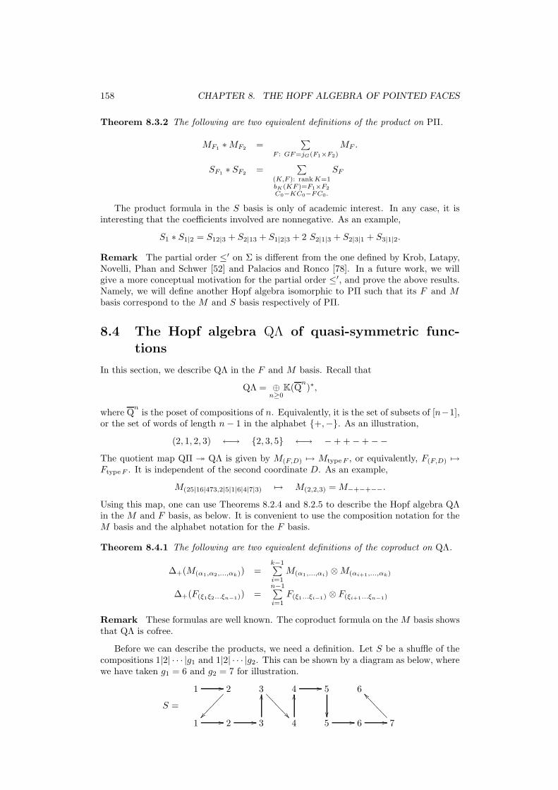
158 CHAPTER 8. THE HOPF ALGEBRA OF POINTED FACES
Theorem 8.3.2 The following are two equivalent definitions of the product on PΠ.
MF1∗MF2
=∑
F : GF=jG(F1×F2)
MF .
SF1∗ SF2
=∑
(K,F ): rankK=1bK(KF )=F1×F2
C0−KC0−FC0.
SF
The product formula in the S basis is only of academic interest. In any case, it isinteresting that the coefficients involved are nonnegative. As an example,
S1 ∗ S1|2 = S12|3 + S2|13 + S1|2|3 + 2 S2|1|3 + S2|3|1 + S3|1|2.
Remark The partial order ≤′ on Σ is different from the one defined by Krob, Latapy,Novelli, Phan and Schwer [52] and Palacios and Ronco [78]. In a future work, we willgive a more conceptual motivation for the partial order ≤′, and prove the above results.Namely, we will define another Hopf algebra isomorphic to PΠ such that its F and M
basis correspond to the M and S basis respectively of PΠ.
8.4 The Hopf algebra QΛ of quasi-symmetric func-
tions
In this section, we describe QΛ in the F and M basis. Recall that
QΛ = ⊕n≥0
K(Qn)∗,
where Qn
is the poset of compositions of n. Equivalently, it is the set of subsets of [n−1],or the set of words of length n− 1 in the alphabet {+,−}. As an illustration,
(2, 1, 2, 3) ←→ {2, 3, 5} ←→ −+ +−+−−
The quotient map QΠ ։ QΛ is given by M(F,D) 7→ MtypeF , or equivalently, F(F,D) 7→FtypeF . It is independent of the second coordinate D. As an example,
M(25|16|473,2|5|1|6|4|7|3) 7→ M(2,2,3) = M−+−+−−.
Using this map, one can use Theorems 8.2.4 and 8.2.5 to describe the Hopf algebra QΛin the M and F basis, as below. It is convenient to use the composition notation for theM basis and the alphabet notation for the F basis.
Theorem 8.4.1 The following are two equivalent definitions of the coproduct on QΛ.
∆+(M(α1,α2,...,αk)) =k−1∑i=1
M(α1,...,αi) ⊗M(αi+1,...,αk)
∆+(F(ξ1ξ2...ξn−1)) =n−1∑i=1
F(ξ1...ξi−1) ⊗ F(ξi+1...ξn−1)
Remark These formulas are well known. The coproduct formula on the M basis showsthat QΛ is cofree.
Before we can describe the products, we need a definition. Let S be a shuffle of thecompositions 1|2| · · · |g1 and 1|2| · · · |g2. This can be shown by a diagram as below, wherewe have taken g1 = 6 and g2 = 7 for illustration.
S =
1 // 2
������
���
3
��>>>
>>>>
4 // 5
��
6
1 // 2 // 3
OO
4
OO
5 // 6 // 7
^^>>>>>>>

8.4. THE HOPF ALGEBRA QΛ OF QUASI-SYMMETRIC FUNCTIONS 159
Now suppose we have two sign sequences ξ = ξ1ξ2 . . . ξg1−1 and η = η1η2 . . . ηg2−1 oflengths g1 − 1 and g2 − 1 respectively. Then, using the shuffle S, we can define a signsequence S(ξ, η) of length g1 + g2 − 1 as illustrated below.
S(ξ, η) =
ξ1 // ξ2
−
������
����
�ξ3
−��?
????
????
ξ4 // ξ5
−
��η1
//η2
//
+
OO
η3
+
OO
η4 η5//
η6//
+
__?????????
Namely, first draw the diagram for the shuffle S. Then put a − sign on the arrows goingdown and a + sign on the arrows going up. The horizontal arrows get labeled ξi or ηi.In the example above, S(ξ, η) = ξ1 − η1η2 +−+ ξ4 − η5η6+.
Theorem 8.4.2 The following are two equivalent definitions of the product on QΛ.
Mα ∗Mβ =∑
γ: γ a quasi-shuffle of α and β
Mγ .
Fξ ∗ Fη =∑
S: S a shuffle of 1| · · · |g1 and 1| · · · |g2
FS(ξ,η),
where ξ and η are sign sequences of length g1 − 1 and g2 − 1 respectively.
For example, in the M basis,
M(2) ∗M(1,1) = M(2,1,1) +M(1,2,1) +M(1,1,2) +M(3,1) +M(1,3).
In the F basis,
F− ∗ F+ = F−−+ + F−++ + F−+− + F+−+ + F++− + F+−−
− //−
������
��
+//
−
−��
+//
+
OO−
−��
−��
+
+??������
−
− ��???
???
+
+
OO+
OO− //
+//
+__??????
− //
−��
+
+
OO
Below each term, we have drawn the diagram from which it arises.In the literature, the product in the F basis is usually described in terms of permu-
tations, by appealing to the fact that QΛ is a quotient of SΛ. The description given inTheorem 8.4.2 in terms of sign sequences may be new. For an expression in terms ofcompositions, see Bertet, Krob, et al [10, Proposition 3.7].
Remark The Loday-Ronco Hopf algebra Y Λ of planar binary trees [56, 57] sits betweenSΛ and QΛ. We claim that there is a Hopf algebra YΠ that lifts Y Λ and sits betweenSΠ and QΠ; see Chapoton [21], Palacios and Ronco [72], Novelli and Thibon [68] andLoday and Ronco [58] for related ideas. There is a similar story for the Hopf algebra oftableau, see Poirier and Reutenauer [78] and also Taskin [97] for related ideas. The waytrees and tableau fit into this theory will be explained in a future work.
Remark The Hopf algebra QΛ satisfies a certain universal property [2]. What can wesay about QΠ and PΠ; do they satisfy any universal properties? This will be explainedin a future work.

160 CHAPTER 8. THE HOPF ALGEBRA OF POINTED FACES

Bibliography
[1] Herbert Abels, The geometry of the chamber system of a semimodular lattice, Order8 (1991), no. 2, 143–158.
[2] Marcelo Aguiar, Nantel Bergeron, and Frank Sottile, Combinatorial Hopf algebrasand generalized Dehn-Sommerville relations, arXiv:math.CO/0310016, to appearin Compos. Math.
[3] Marcelo Aguiar and Frank Sottile, Cocommutative Hopf algebras of permutationsand trees, J. Algebraic Combin. 22 (2005), 451–470.
[4] , Structure of the Malvenuto-Reutenauer Hopf algebra of permutations, Adv.Math. 191 (2005), no. 2, 225–275.
[5] , Structure of the Loday-Ronco Hopf algebra of trees, J. Algebra 295 (2006),no. 2, 473–511.
[6] M. D. Atkinson, Solomon’s descent algebra revisited, Bull. London Math. Soc. 24
(1992), no. 6, 545–551.
[7] Francois Bergeron, Nantel Bergeron, Robert B. Howlett, and Donald E. Taylor, Adecomposition of the descent algebra of a finite Coxeter group, J. Algebraic Combin.1 (1992), no. 1, 23–44.
[8] Nantel Bergeron, Christophe Hohlweg, Mercedes Rosas, and Mike Zabrocki,Grothendieck bialgebras, Partition lattices and symmetric functions in noncom-mutative variables, arXiv:math.CO/0506360.
[9] Nantel Bergeron and Mike Zabrocki, The Hopf algebras of symmetric functionsand quasisymmetric functions in non-commutative variables are free and cofree,arXiv:math.CO/0509265.
[10] K. Bertet, D. Krob, M. Morvan, J.-C. Novelli, H. D. Phan, and J.-Y. Thibon, Anoverview of Λ-type operations on quasi-symmetric functions, Comm. Algebra 29
(2001), no. 9, 4277–4303, Special issue dedicated to Alexei Ivanovich Kostrikin.
[11] T. Patrick Bidigare, Hyperplane arrangement face algebras and their associatedMarkov chains, Ph.D. thesis, University of Michigan, 1997.
[12] T. Patrick Bidigare, Phil Hanlon, and Daniel N. Rockmore, A combinatorial de-scription of the spectrum for the Tsetlin library and its generalization to hyperplanearrangements, Duke Math. J. 99 (1999), no. 1, 135–174.
[13] Louis J. Billera, Kenneth S. Brown, and Persi Diaconis, Random walks and planearrangements in three dimensions, Amer. Math. Monthly 106 (1999), no. 6, 502–524.
161

162 BIBLIOGRAPHY
[14] Anders Bjorner, Michel Las Vergnas, Bernd Sturmfels, Neil White, and Gunter M.Ziegler, Oriented matroids, Encyclopedia of Mathematics and its Applications,vol. 46, Cambridge University Press, Cambridge, 1993.
[15] Dieter Blessenohl and Manfred Schocker, Noncommutative character theory of thesymmetric group, Imperial College Press, London, 2005.
[16] Nicolas Bourbaki, Elements de mathematique, Masson, Paris, 1981, Groupes etalgebres de Lie. Chapitres 4, 5 et 6. [Lie groups and Lie algebras. Chapters 4, 5and 6].
[17] Kenneth S. Brown, Buildings, Springer-Verlag, New York, 1989.
[18] , Semigroups, rings, and Markov chains, J. Theoret. Probab. 13 (2000),no. 3, 871–938.
[19] Kenneth S. Brown and Persi Diaconis, Random walks and hyperplane arrangements,Ann. Probab. 26 (1998), no. 4, 1813–1854.
[20] P. Cartier, On the structure of free Baxter algebras, Advances in Math. 9 (1972),253–265.
[21] Frederic Chapoton, Algebres de Hopf des permutahedres, associahedres et hyper-cubes, Adv. Math. 150 (2000), no. 2, 264–275.
[22] George E. Cooke and Ross L. Finney, Homology of cell complexes, Princeton Uni-versity Press, Princeton, N.J., 1967, Based on lectures by Norman E. Steenrod.
[23] H. S. M. Coxeter, The complete enumeration of finite groups of the form r2i =(rirj)
kij = 1, J. London Math. Soc. 10 (1935), 21–25.
[24] Peter Doubilet, On the foundations of combinatorial theory. VII. Symmetric func-tions through the theory of distribution and occupancy, Studies in Appl. Math. 51
(1972), 377–396.
[25] Andreas W. M. Dress and Rudolf Scharlau, Gated sets in metric spaces, Aequa-tiones Math. 34 (1987), no. 1, 112–120.
[26] Gerard Duchamp, Florent Hivert, and Jean-Yves Thibon, Some generalizationsof quasi-symmetric functions and noncommutative symmetric functions, Formalpower series and algebraic combinatorics (Moscow, 2000), Springer, Berlin, 2000,pp. 170–178.
[27] , Noncommutative symmetric functions. VI. Free quasi-symmetric functionsand related algebras, Internat. J. Algebra Comput. 12 (2002), no. 5, 671–717.
[28] Gerard Duchamp, Alexander Klyachko, Daniel Krob, and Jean-Yves Thibon, Non-commutative symmetric functions. III. Deformations of Cauchy and convolutionalgebras, Discrete Math. Theor. Comput. Sci. 1 (1997), no. 1, 159–216, Lie compu-tations (Marseille, 1994).
[29] Richard Ehrenborg, On posets and Hopf algebras, Adv. Math. 119 (1996), no. 1,1–25.
[30] Loıc Foissy, Bidendriform bialgebras, trees, and free quasi-symmetric functions,arXiv:math.RA/0505207.
[31] William Fulton, Young tableaux, London Mathematical Society Student Texts,vol. 35, Cambridge University Press, Cambridge, 1997, With applications to rep-resentation theory and geometry.

BIBLIOGRAPHY 163
[32] A. M. Garsia and C. Reutenauer, A decomposition of Solomon’s descent algebra,Adv. Math. 77 (1989), no. 2, 189–262.
[33] David D. Gebhard and Bruce E. Sagan, A chromatic symmetric function in non-commuting variables, J. Algebraic Combin. 13 (2001), no. 3, 227–255.
[34] Ladnor Geissinger, Hopf algebras of symmetric functions and class functions, Com-binatoire et representation du groupe symetrique (Actes Table Ronde C.N.R.S.,Univ. Louis-Pasteur Strasbourg, Strasbourg, 1976), Springer, Berlin, 1977, pp. 168–181. Lecture Notes in Math., Vol. 579.
[35] Israel M. Gelfand, Daniel Krob, Alain Lascoux, Bernard Leclerc, Vladimir S. Re-takh, and Jean-Yves Thibon, Noncommutative symmetric functions, Adv. Math.112 (1995), no. 2, 218–348.
[36] Ira M. Gessel, Multipartite P -partitions and inner products of skew Schur functions,Combinatorics and algebra (Boulder, Colo., 1983), Amer. Math. Soc., Providence,RI, 1984, pp. 289–317.
[37] Curtis Greene, On the Mobius algebra of a partially ordered set, Advances in Math.10 (1973), 177–187.
[38] Pierre Antoine Grillet, Semigroups. an introduction to the structure theory, Mono-graphs and Textbooks in Pure and Applied Mathematics, vol. 193, Marcel DekkerInc., New York, 1995.
[39] Larry C. Grove and Clark T. Benson, Finite reflection groups, second ed., GraduateTexts in Mathematics, vol. 99, Springer-Verlag, New York, 1985.
[40] Michiel Hazewinkel, The algebra of quasi-symmetric functions is free over the in-tegers, Adv. Math. 164 (2001), no. 2, 283–300.
[41] , Generalized overlapping shuffle algebras, J. Math. Sci. (New York) 106
(2001), no. 4, 3168–3186, Pontryagin Conference, 8, Algebra (Moscow, 1998).
[42] , Symmetric functions, noncommutative symmetric functions, and qua-sisymmetric functions, Acta Appl. Math. 75 (2003), no. 1-3, 55–83, Monodromyand differential equations (Moscow, 2001).
[43] , Symmetric functions, noncommutative symmetric functions and quasisym-metric functions. II, Acta Appl. Math. 85 (2005), no. 1-3, 319–340.
[44] F. Hivert, J.-C. Novelli, and J.-Y. Thibon, Commutative Hopf algebras of permu-tations and trees, arXiv:math.CO/0502456.
[45] Florent Hivert, Combinatoire des fonctions quasi-symetriques, Ph.D. thesis, Uni-versite de Marne-la-Vallee, 1999.
[46] Michael E. Hoffman, Quasi-shuffle products, J. Algebraic Combin. 11 (2000), no. 1,49–68.
[47] James E. Humphreys, Reflection groups and Coxeter groups, Cambridge Studies inAdvanced Mathematics, vol. 29, Cambridge University Press, Cambridge, 1990.
[48] S. A. Joni and G.-C. Rota, Coalgebras and bialgebras in combinatorics, Umbralcalculus and Hopf algebras (Norman, Okla., 1978), Contemp. Math., vol. 6, Amer.Math. Soc., Providence, R.I., 1982, pp. 1–47.
[49] Christian Kassel, Quantum groups, Springer-Verlag, New York, 1995.

164 BIBLIOGRAPHY
[50] Fritz Klein-Barmen, Uber eine weitere Verallgemeinerung des Verbandsbegriffes,Math. Z. 46 (1940), 472–480.
[51] D. Krob, B. Leclerc, and J.-Y. Thibon, Noncommutative symmetric functions. II.Transformations of alphabets, Internat. J. Algebra Comput. 7 (1997), no. 2, 181–264.
[52] Daniel Krob, Matthieu Latapy, Jean-Christophe Novelli, Ha Duong Phan, andSylvaine Schwer, Pseudo-permutations I : First combinatorial and lattice properties,Paper presented at 13th FPSAC (Formal power series and algebraic combinatorics)Arizona State University, Arizona – USA, May 20 – 26, 2001.
[53] Daniel Krob and Jean-Yves Thibon, Noncommutative symmetric functions. IV.Quantum linear groups and Hecke algebras at q = 0, J. Algebraic Combin. 6 (1997),no. 4, 339–376.
[54] , Noncommutative symmetric functions. V. A degenerate version of Uq(glN ),Internat. J. Algebra Comput. 9 (1999), no. 3-4, 405–430, Dedicated to the memoryof Marcel-Paul Schutzenberger.
[55] Jean-Louis Loday and Marıa O. Ronco, On the structure of cofree Hopf algebras,arXiv:math.QA/0405330, to appear in J. f. reine u. angew. Mathematik (Crelle’sJournal).
[56] , Hopf algebra of the planar binary trees, Adv. Math. 139 (1998), no. 2,293–309.
[57] , Order structure on the algebra of permutations and of planar binary trees,J. Algebraic Combin. 15 (2002), no. 3, 253–270.
[58] , Trialgebras and families of polytopes, Homotopy theory: relations withalgebraic geometry, group cohomology, and algebraic K-theory, Contemp. Math.,vol. 346, Amer. Math. Soc., Providence, RI, 2004, pp. 369–398.
[59] I. G. Macdonald, Symmetric functions and Hall polynomials, second ed., TheClarendon Press Oxford University Press, New York, 1995, With contributionsby A. Zelevinsky, Oxford Science Publications.
[60] Swapneel Mahajan, Shuffles, shellings and projections, Ph.D. thesis, Cornell Uni-versity, 2002.
[61] Claudia Malvenuto, Produits et coproduits des fonctions quasi-symetriques et del’algebre des descents, Ph.D. thesis, Laboratoire de combinatoire et d’informatiquemathematique (LACIM), Univ. du Quebec a Montreal, 1994.
[62] Claudia Malvenuto and Christophe Reutenauer, Duality between quasi-symmetricfunctions and the Solomon descent algebra, J. Algebra 177 (1995), no. 3, 967–982.
[63] Arnaldo Mandel, Topology of oriented matroids, Ph.D. thesis, University of Water-loo, 1982.
[64] John W. Milnor and John C. Moore, On the structure of Hopf algebras, Ann. ofMath. (2) 81 (1965), 211–264.
[65] Susan Montgomery, Hopf algebras and their actions on rings, CBMS Regional Con-ference Series in Mathematics, vol. 82, Published for the Conference Board of theMathematical Sciences, Washington, DC, 1993.
[66] Bernhard Muhlherr, Some contributions to the theory of buildings based on the gateproperty, Ph.D. thesis, Eberhard-Karls-Universitat zu Tubingen, 1994.
BIBLIOGRAPHY 165
[67] Jean-Christophe Novelli and Jean-Yves Thibon, A Hopf algebra of parking func-tions, arXiv:math.CO/0312126.
[68] , Construction of dendriform trialgebras, arXiv:math.CO/0510218.
[69] Jean-Christophe Novelli and Jean-Yves Thibon, Hopf algebras and dendriformstructures arising from parking functions, arXiv:math.CO/0511200.
[70] Peter Orlik and Louis Solomon, Unitary reflection groups and cohomology, Invent.Math. 59 (1980), no. 1, 77–94.
[71] Peter Orlik and Hiroaki Terao, Arrangements of hyperplanes, Grundlehren derMathematischen Wissenschaften, vol. 300, Springer-Verlag, Berlin, 1992.
[72] Patricia Palacios and Marıa O. Ronco, Weak Bruhat order on the set of faces ofthe permutahedra, arXiv:math.CO/0404352.
[73] Frederic Patras and Christophe Reutenauer, Lie representations and an algebracontaining Solomon’s, J. Algebraic Combin. 16 (2002), no. 3, 301–314 (2003).
[74] , On descent algebras and twisted bialgebras, Mosc. Math. J. 4 (2004), no. 1,199–216, 311.
[75] Frederic Patras and Manfred Schocker, Twisted descent algebras and the Solomon-Tits algebra, Adv. Math. 199 (2006), no. 1, 155–184.
[76] Mario Petrich, A construction and a classification of bands, Math. Nachr. 48 (1971),263–274.
[77] , Lectures in semigroups, John Wiley & Sons, London-New York-Sydney,1977.
[78] Stephane Poirier and Christophe Reutenauer, Algebres de Hopf de tableaux, Ann.Sci. Math. Quebec 19 (1995), no. 1, 79–90.
[79] Daniel Quillen, Rational homotopy theory, Ann. of Math. (2) 90 (1969), 205–295.
[80] Nathan Reading, Lattice congruences of the weak order, arXiv:math.CO/0401404.
[81] , Lattice congruences, fans and Hopf algebras, J. Combin. Theory Ser. A110 (2005), no. 2, 237–273.
[82] Christophe Reutenauer, Free Lie algebras, London Mathematical Society Mono-graphs. New Series, vol. 7, The Clarendon Press Oxford University Press, NewYork, 1993, Oxford Science Publications.
[83] Mercedes H. Rosas and Bruce E. Sagan, Symmetric functions in noncommutingvariables, Trans. Amer. Math. Soc. 358 (2006), no. 1, 215–232 (electronic).
[84] Bruce E. Sagan, The symmetric group, second ed., Graduate Texts in Mathemat-ics, vol. 203, Springer-Verlag, New York, 2001, Representations, combinatorial al-gorithms, and symmetric functions.
[85] Franco V. Saliola, The Face Semigroup Algebra of a Hyperplane Arrangement,arXiv:math.RA/0511717.
[86] Rudolf Scharlau, Metrical shellings of simplicial complexes, European J. Combin.6 (1985), no. 3, 265–269.
[87] William R. Schmitt, Hopf algebras of combinatorial structures, Canad. J. Math. 45
(1993), no. 2, 412–428.

166 BIBLIOGRAPHY
[88] , Incidence Hopf algebras, J. Pure Appl. Algebra 96 (1994), no. 3, 299–330.
[89] Manfred Schocker, The descent algebra of the symmetric group, Representations offinite dimensional algebras and related topics in Lie theory and geometry, FieldsInst. Commun., vol. 40, Amer. Math. Soc., Providence, RI, 2004, pp. 145–161.
[90] Maurice-Paul Schutzenberger, Sur certains treillis gauches, C. R. Acad. Sci. Paris224 (1947), 776–778.
[91] Louis Solomon, The Burnside algebra of a finite group, J. Combinatorial Theory 2
(1967), 603–615.
[92] , A Mackey formula in the group ring of a Coxeter group, J. Algebra 41
(1976), no. 2, 255–264.
[93] Richard P. Stanley, Enumerative combinatorics. Vol. 1, Cambridge Studies in Ad-vanced Mathematics, vol. 49, Cambridge University Press, Cambridge, 1997, witha foreword by Gian-Carlo Rota, corrected reprint of the 1986 original.
[94] , Enumerative combinatorics. Vol. 2, Cambridge Studies in Advanced Math-ematics, vol. 62, Cambridge University Press, Cambridge, 1999, With a forewordby Gian-Carlo Rota and appendix 1 by Sergey Fomin.
[95] Moss E. Sweedler, Hopf algebras, Mathematics Lecture Note Series, W. A. Ben-jamin, Inc., New York, 1969.
[96] Mitsuhiro Takeuchi, Free Hopf algebras generated by coalgebras, J. Math. Soc. Japan23 (1971), 561–582.
[97] Muge Taskin, Properties of four partial orders on standard Young tableaux,arXiv:math.CO/0509174.
[98] Jean-Yves Thibon, Lectures on noncommutative symmetric functions, Interactionof combinatorics and representation theory, MSJ Mem., vol. 11, Math. Soc. Japan,Tokyo, 2001, pp. 39–94.
[99] Jacques Tits, Buildings of spherical type and finite BN-pairs, Springer-Verlag,Berlin, 1974, Lecture Notes in Mathematics, Vol. 386.
[100] M. C. Wolf, Symmetric functions of noncommuting elements, Duke Math. J. (1936),626–637.
[101] Thomas Zaslavsky, Facing up to arrangements: face-count formulas for partitionsof space by hyperplanes, Mem. Amer. Math. Soc. 1 (1975), no. 154, vii+102 pp.
[102] Andrey V. Zelevinsky, Representations of finite classical groups, Lecture Notes inMathematics, vol. 869, Springer-Verlag, Berlin, 1981, A Hopf algebra approach.
[103] Gunter M. Ziegler, Lectures on polytopes, Graduate Texts in Mathematics, vol. 152,Springer-Verlag, New York, 1995.

AUTHOR INDEX 167
Author Index
Abels, Herbert, 1, 24Aguiar, Marcelo, 10, 22, 27, 33, 35, 37,
50, 52, 55, 70, 129, 132, 139,141, 159
Atkinson, M. D., 23
Benson, Clark T., 4Bergeron, Francois, 23Bergeron, Nantel, 23, 78, 80, 152, 159Bertet, Karell, 31, 159Bidigare, T. Patrick, 7, 8, 11, 20Billera, Louis J., 8, 15Bjorner, Anders, 1–3Blessenohl, Dieter, 29Bourbaki, Nicolas, 4Brown, Kenneth S., 2, 4, 7, 8, 11, 12, 15,
20, 24, 25, 43
Cartier, Pierre, 31Chapoton, Frederic, 78, 82, 159Cooke, George E., 1Coxeter, H.S.M., 5
Diaconis, Persi, 8, 15Doubilet, Peter, 69Dress, Andreas W. M., 1Duchamp, Gerard, 32, 129, 132
Edmonds, J., 3Ehrenborg, Richard, 27, 31
Finney, Ross L., 1Foissy, Loıc, 129Fulton, William, 29
Garsia, Adriano M., 23Gebhard, David D., 60, 78Geissinger, Ladnor, 30, 38, 75Gelfand, Israel M., 32, 38, 75Gessel, Ira M., 31, 32, 38, 75, 151Greene, Curtis, 20Grillet, Pierre Antoine, 11Grove, Larry C., 4
Hanlon, Phil, 8, 20Hazewinkel, Michiel, 29, 31, 32Hivert, Florent, 32, 78, 80, 129, 132Hoffman, Michael E., 31, 38, 75, 151Hohlweg, Christophe, 78Howlett, Robert B., 23Humphreys, James E., 4, 37
Joni, S. A., 27
Kassel, Christian, 27Klein-Barmen, Fritz, 12Klyachko, Alexander, 32Krob, Daniel, 23, 31, 32, 38, 75, 158, 159
Las Vergnas, Michel, 1–3Lascoux, Alain, 32, 38, 75Latapy, Matthieu, 158Leclerc, Bernard, 23, 32, 38, 75Loday, Jean-Louis, 28, 129, 136, 159
Macdonald, Ian G., 29, 71Mahajan, Swapneel, 1, 4, 15, 23, 24, 46,
50Malvenuto, Claudia, 29, 31, 32, 37, 38,
70, 75, 129, 132, 151Mandel, Arnaldo, 3Milnor, John W., 28, 30, 32Montgomery, Susan, 27Moore, John C., 28, 30, 32Morvan, Michel, 31, 159Muhlherr, Bernhard, 1
Novelli, Jean-Christophe, 31, 80, 158, 159
Orlik, Peter, 2, 21
Palacios, Patricia, 78, 158, 159Patras, Frederic, 78, 129Petrich, Mario, 11Phan, Ha Duong, 31, 158, 159Poirier, Stephane, 129, 132, 159
Quillen, Daniel, 28, 30
Reading, Nathan, 37Reiner, Victor, 21Retakh, Vladimir S., 32, 38, 75Reutenauer, Christophe, 23, 31, 32, 78,
129, 132, 159Rockmore, Daniel N., 8, 20Ronco, Marıa O., 28, 78, 129, 136, 158,
159Rosas, Mercedes H., 60, 69, 78Rota, Gian-Carlo, 27
Sagan, Bruce E., 29, 60, 69, 78Saliola, Franco V., 3Scharlau, Rudolf, 1Schmitt, William R., 27Schocker, Manfred, 23, 29, 78Schwer, Sylvaine, 158Schutzenberger, Maurice-Paul, 11, 12

168 BIBLIOGRAPHY
Solomon, Louis, 7, 20, 21, 23Sottile, Frank, 10, 22, 27, 33, 35, 37, 50,
52, 55, 70, 129, 132, 139, 141,159
Stanley, Richard P., 20, 29, 31, 68, 71Sturmfels, Bernd, 1–3Sweedler, Moss E., 27, 28
Takeuchi, Mitsuhiro, 28Taskin, Muge, 159Taylor, Donald E., 23Terao, Hiroaki, 2, 21Thibon, Jean-Yves, 23, 31, 32, 38, 75,
80, 129, 132, 159Tits, Jacques, 1, 4, 5, 24
White, Neil, 1–3Wolf, M. C., 78
Zabrocki, Michael, 78, 80, 152Zaslavsky, Thomas, 20Zelevinsky, Andrei V., 30, 38, 75Ziegler, Gunter M., 1–3

NOTATION INDEX 169
Notation Index
algebra(KL)W , 23(KΣ)W , 7, 22KL, 14, 20, 64KL, 71KΣ, 7, 14, 64
basisH , K, M , F , 59, 66, 130R, S, 59, 130h, m, 59, 66q, p, 59, 64, 66, 71
bilinear formon (KL)W , 23on (KΣ)W , 11, 22on KL, 19on KQ, 17, 61on KΣ, 11, 19
chamberC, D, E, ii
coalgebraC, 27
compositionα, β and γ, 31
elements of an algebraσT , 7dT , 7
faceF , G, H , K, N , P , Q, ii
fieldK, ii
flatX , Y , ii
gradedalgebraAZ , AL, AZ∗ and AL∗ , 126P∆, 119PΓ, 120SΓ, 124P , Q, S, R, N andM, 118
coalgebraAZ , AL, AZ∗ and AL∗ , 110P∆, 100PΓ, 101Q(V ), 27SΓ, 108P , Q, S, R, N andM, 98
group
W , 4WS\T , 7Sn, 8Zn−12 , 56
group generatorssi, 5sH, 4, 8
half-spaceH+i , H−
i , 2Hopf algebra
MΠ of set compositionsH basis, 77, 79, 82, 102, 121
NΛ of noncommutative symmetricfunctions, 29, 38
H basis, 32K basis, 32, 119
NΠ of fully nested set compositionsH basis, 77, 79, 84, 105, 123
PΠ of set compositionsM basis, 77, 79, 82, 101, 119, 157S basis, 157
QΛ of quasi-symmetric functions, 29,31, 38
F basis, 31, 158M basis, 31, 100, 119, 158
QΠ of fully nested set compositionsF basis, 153M basis, 77, 79, 84, 104, 122, 153S basis, 153
RΛ of permutations, 130RΠ of pairs of permutations, 130H basis, 146K basis, 77, 79, 88
SΛ of permutationsF basis, 136M basis, 137
SΠ of pairs of permutationsF basis, 77, 79, 87, 107, 124, 133M basis, 137S basis, 142
Y Λ of planar binary trees, 159Λ of symmetric functions, 29, 38, 66h basis, 29m basis, 29p basis, 29q basis, 66, 72
ΠL and ΠL∗ of set partitionsh basis, 60, 77, 79, 86m basis, 60, 77, 79, 85p basis, 60

170 BIBLIOGRAPHY
q basis, 60ΠZ∗ of fully nested set partitionsm basis, 77, 79, 87
ΠZ of fully nested set partitionsh basis, 77, 79, 87
hyperplaneHi, 2
luneL, M , ii
mapS antipode, 28∆ coproduct, 27Des, 42, 54, 58GDes, 43, 54, 58GRoad, 43Φ, 60, 63Ψ, 61Road, 42, 60, 109, 125Θ, 44, 54, 58, 60, 109, 126Υ, 63base, 63, 104, 122base∗, 62, 106, 123deg, 89, 112des, 7, 46, 55, 58dist, 1ǫ counit, 28gdes, 47, 55, 58lune, 13, 53, 57, 62, 111, 127lune∗, 63, 111, 127φ, 65, 66, 78ψ, 65, 78rank, 89, 154reg, 14, 63road, 47st, 80supp, 12, 53, 56, 62, 111, 127supp∗, 63, 111, 127θ, 47, 55, 58type, 39, 54, 57, 90ζ, 19zone, 14, 63j, j, j′, j′′ join, 133l length, 6, 46, 55m product, 28s switch, 60, 88u unit, 28x·, 17break bK
axioms, 89, 111example, 91, 92, 94, 96, 135
join jGaxioms, 112, 127
example, 113–116, 135minimum gallery
E −D − C, 4
numberRλµ, 66, 68|λ|, 67, 68dist(C,D), 2κ, 72parts(α), 32parts(λ), 31cX , 19, 21cx, 19cλµ, 31mij , 5nX , 20, 21, 23, 71zλ, 71
orbit space(C × C)W , 39LW , 39QW , 39ΣW , 39ZW , 39
partial order≤ on W , 6≤, ≤′ and � on C × C, 41, 131≤, ≤′ and � on Q, 42, 152≤′ on Σ, 157≤b on C, 40, 131≤rb on W , 6≤rb on C, 131, 136
partitionλ, µ and ρ, 29
pointed face(F,D), (P,C), ii
posetW , 6, 39C × C, 39L, 12Ln, 53, 56L, 21, 40Ln, 29, 54, 57
Q, 13, 39Qn, 53, 57Q, 7, 21, 39Qn, 31, 54, 57
Σ, 1, 2, 4, 12Σn, 53, 56Sn, 10Z, 13, 40Zn, 53, 57
set

NOTATION INDEX 171
S+w (u × v), 141S−w (u × v), 141, 147S0w(u × v), 141S0w(x), S+
w (x) and S−w (x), 51
C, 1CF , 2, 49, 89, 112Cx, 12Left, Middle and Right, 97, 101, 103,
105OT , 66Oα, 68Oλ, 66, 68, 71ShT , 49, 56ΣF , 2ΣK , 89, 112ΣT , 49Σx, Lx, Zx, 17Z′ of lunar regions, 14, 15, 63link(F ), 2reg(F,D), 15reg(x, c), 14star(F ), 2
sign sequenceS(ξ, η), 159
subsetS, T , U , V , ii
vector spaceP (C), 28V , 27KP , iiKP ∗, ii

172 BIBLIOGRAPHY
Subject Index
actionof the Coxeter group, 4, 39simply transitive, 4, 40type-preserving, 5
adjoint functors, 45, 48algebra, 116
associative, 117free, 29, 32, 129from axioms, 116iterated product, 28primitive idempotent in, 23, 64, 71radical of, 11, 20, 23semigroup, 7semisimple, 20, 23, 64, 71
alphabet, 56, 158antipode, see Hopf algebraapartment, see buildingascent
of a pair of chambers, 42of an element of W , 47
axiomalgebra, 112coalgebra, 89, 96compatible, 79projection, 90, 113
barsbig, 53, 83small, 53, 83
basiscanonical, 59dual, 30, 60, 66, 132orthogonal, 64, 71
bialgebra, 28bijection
chambers in two star regions, 13, 25controlling coassociativity, 97lunes and lunar regions, 16
bilinear forminvariant, 19nondegenerate, 20, 23on faces, 19on flats, 19on orbit space of flats, 23on pointed faces, 17, 61on subsets or compositions, 22radical of, 11, 20, 23
braid arrangement, 8, 52Bruhat order
of permutations, 10weak left, 6, 37, 131
weak right, 6, 131building, 24
apartment, 24
chamberadjacent, 1fundamental, 4, 40, 49, 92of a LRB, 12of a projection poset, 24of a regular cell complex, 1of a simplicial complex, 1of an arrangement, 2pair of, 6wall of, 3, 15
chamber complex, 39coalgebra
coassociative, 96cofree, 27, 129, 152, 158connected, 27coradical filtration of, 28, 145, 154coradical of, 28deconcatenation coproduct, 27from axioms, 96iterated coproduct, 27primitive element in, 28, 30, 32, 139,
145, 154universal property, 27
cofree coalgebra, see coalgebracoinvariants
maps to, 69of the W action, 37
commutative diagramof type A, 77related to C × C, 58related to W , 65
composition, 31, 54, 90, 113, 158bilinear form on, 22internal product, 32partial order on, 31, 54quasi-shuffle of, 31, 159support of, 31weak, 31, 32
convex, 1, 44, 45convolution, 28coordinate arrangement, 56coradical, see coalgebracoradical filtration, see coalgebraCoxeter
complex, 4diagram, 5
of type A×(n−1)1 , 95
SUBJECT INDEX 173
of type An−1, 5, 92, 135of type Bn, 5
group, 5, 39cartesian product of, 7exponent, 21invariant theory, 21
of type A×(n−1)1 , 56, 95, 116
of type An−1, 8, 52, 92, 114presentation, 5, 8, 56
parabolic subgroup, 7, 21, 37, 51system, 5, 39
criterion on radicals, 11
deconcatenation coproduct, see coalge-bra
dendriform trialgebra, 78descent
of a pair of chambers, 42of a pair of permutations, 54of a pair of words, 58of a permutation, 55of a word, 58of an element of W , 7, 46
descent algebra, 7, 23structure constants, 22
distance, see mapdistributive lattice, see lattice
exponent, see Coxeter groupexternal structure, 56, 72, 76
facebilinear form on, 19fundamental, 113global vertex of, 99join of, 121joinable, 2local vertex of, 99of a LRB, 12of a simplicial complex, 1of an arrangement, 2opposite, 2, 43, 53, 56partial order on, 12, 157quasi-shuffle of, 119type of, 5, 9
facet, see hyperplane arrangementflat
bilinear form on, 19global vertex of, 99join of, 127local vertex of, 99of a LRB, 12of an arrangement, 3partial order on, 12quasi-shuffle of, 127
free algebra, see algebrafree Lie algebra, 32free LRB, see left regular band (LRB)
gallery, 1connected, 1, 2, 4distance, 1, 4, 6metric, 1, 4, 6, 49, 91minimum, 1, 2, 4, 6, 8, 41–43
gate property, 1application of, 45, 50–52, 137, 140,
147of hyperplane arrangements, 3
global ascentof a pair of permutations, 145, 148
global descentof a pair of chambers, 43of a pair of permutations, 54, 137,
139, 145, 148of a pair of words, 58of a permutation, 55of a word, 58of an element of W , 47
global vertexof faces, 99of flats, 99of fully nested set compositions, 83of fully nested set partitions, 86of lunes, 99of pointed faces, 99of set compositions, 80of set partitions, 85
great circle, 15
half-spaceclosed, 2, 15open, 2
Hopf algebra, 27antipode, 28, 133examples, 29, 77, 79self-dual, 29, 129structural results, 29, 80structure maps, 28universal property, 159
hyperplaneseparates, 2, 4, 10, 42, 44supporting, 2, 15
hyperplane arrangement, 2as a LRB, 13central, 2chamber of, 2essential, 2face of, 2facet of, 2

174 BIBLIOGRAPHY
flat of, 3lunar region in, 15, 44, 135product in, 2projection map in, 4rank 3 example, 15subarrangement, 15
ideal, see semigroupinner product, 4, 30, 60, 66internal product
composition, 32set composition, 9set partition, 9
internal structure, 72, 75, 78intersection lattice, see latticeinvariant theory, see Coxeter groupinvariants
maps from, 67of the W action, 37
inversions, see permutationisomorphism
ΛL and ΛL∗ , 66ΠL and ΠL∗ , 60
iterated coproduct, see coalgebraiterated product, see algebra
joinin a poset, 39of Coxeter complexes, 7, 92of faces, 121of flats, 127of LRBs, 17of lunes, 127of nested set compositions, 83of nested set partitions, 86of pointed faces, 123of set compositions, 80of set partitions, 85of simplicial complexes, 2
joinable, see face
latticedistributive, 24intersection, 3, 21modular, 24of flats, 3semilattice, 12, 39
left regular band (LRB), 12chamber of, 12face of, 12family of, 76flat of, 12free, 13, 16, 21link in, 17lune in, 13, 99
nonassociative, 24product of, 17quotient, 17star region in, 17sub, 17
length, see maplink
in a Coxeter complex, 7, 92, 135in a LRB, 17in a simplicial complex, 2
local vertexof faces, 99of flats, 99of lunes, 99of nested set compositions, 83of nested set partitions, 86of pointed faces, 99of set compositions, 80of set partitions, 85
LRB, see left regular bandlunar region
base of, 15in a LRB, 14in an arrangement, 15, 44, 50, 135
luneglobal vertex of, 99in a LRB, 13, 99join of, 127local vertex of, 99quasi-shuffle of, 127
Mobius function, see posetmap
distance, 6, 39, 57length, 6, 46opposite, 43, 53, 56order preserving, 12, 13, 41–45standardization, 80support, 3, 12switch, 60, 88
on the H basis, 148on the M basis, 141
matroid, 3meet, see posetminimum gallery, see gallerymodular lattice, see lattice
nilpotent, 20, 23, 28nonassociative, 11, 24noncommutative, 32, 60, 78
open questions, 15, 18, 21, 46, 79, 133opposite, see face, maporbit, 39order complex, 24

SUBJECT INDEX 175
order preserving, see maporiented matroid, 2, 3, 15, 56
pair, see chamber,permutationparabolic subgroup, see Coxeterpartial order
compositions, 31, 54faces, 12, 157flats, 12fully nested set compositions, 53fully nested set partitions, 53pairs of chambers, 41pairs of permutations, 131partitions, 29, 54permutations, 10pointed faces, 13, 42, 152set compositions, 9set partitions, 9
partition, 29, 54, 66false-shuffle of, 29partial order on, 29, 54quasi-shuffle of, 29shuffle of, 29
permutahedron, 78permutation
Bruhat order on, 10descent of, 55global descent of, 55inversions of, 10pair of, 79
pointed face, 13bilinear form on, 17global vertex of, 99join of, 123local vertex of, 99partial order on, 13, 42quasi-shuffle of, 122
polygon, 2polynomial realization, 78poset
Mobius function of, 20, 21cartesian product of, 92family of, 89, 112graded, 89, 112join in a, 39meet in a, 39quotient, 40, 54, 57
power series, 29, 31presentation, see Coxeter groupprimitive element, see coalgebraprimitive idempotent, see algebraprojection map
in a Coxeter complex, 5, 91in an arrangement, 4
in type A, 9, 53
in type A×(n−1)1 , 56
projection posetdefinition, 24family of, 96, 98, 116, 118in algebra axioms, 113in coalgebra axioms, 90
pure, see regular cell complex
quasi-shuffleof compositions, 31, 159of faces, 119of flats, 127of fully nested set compositions, 83of fully nested set partitions, 86of lunes, 127of partitions, 29of pointed faces, 122of set compositions, 80
geometric meaning, 103, 120of set partitions, 85
radical, see algebrarandom walk, 20rank, 5, 89, 112reflection
arrangement, 4group, 4
regular cell complex, 1, 3gallery connected, 1pure, 1strongly connected, 1
representation theory, 29
section to a surjective map, 45, 49, 113self-dual, see Hopf algebrasemigroup, 2, 5, 12, see algebra
ideal in, 2, 13semilattice, see latticesemisimple, see algebraset composition, 9, 53, 79, 80
fully nested, 53, 79, 83internal product, 9nested, 53, 83partial order on, 9
set partition, 9, 53, 60, 79, 85fully nested, 53, 79, 86internal product, 9nested, 53, 86partial order on, 9
shufflefor a Coxeter group, 49of compositions, 31of partitions, 29of set compositions, 56, 80, 159

176 BIBLIOGRAPHY
geometric meaning, 103, 120sign sequence, 2, 56
stacked, 57simplicial complex, 1, 3
gallery connected, 1, 39join of, 2, 92link in, 2pure, 1, 39strongly connected, 1
simply transitive, see actionSolomon’s descent algebra, see descent
algebrastandardize, see mapstar region
in a complex, 1, 43, 47in a LRB, 17
strongly connected, see regular cell com-plex
support, see mapsupporting hyperplane, see hyperplanesymmetric group
Bruhat order on, 10combinatorial approach, 52geometric approach, 8presentation, 8
tableau, 159trees, 159type, see face,vertextype-preserving, see action
universal property, see coalgebra, Hopfalgebra
vertexfundamental, 119, 135of a set, 80type of, 5, 9
wall, see chamberweak composition, see composition
zone, 14