coversheet - los alamos national laboratory: mcnp home … · mcnp6 for criticality accident alarm...

LA-UR-12-25545Approved for public release; distribution is unlimited.

Title: MCNP6 for Criticality Accident Alarm Systems -- A Primer

Author(s): Kiedrowski, Brian C.

Intended for: MCNP WebsiteReportWeb

Disclaimer:Los Alamos National Laboratory, an affirmative action/equal opportunity employer,is operated by the Los Alamos National Security, LLC for the National NuclearSecurity Administration of the U.S. Department of Energy under contract DE-AC52-06NA25396. By approving this article, the publisher recognizes that the U.S. Government retains nonexclusive, royalty-free license to publish or reproduce the published form of this contribution, or to allow others to do so, for U.S. Government purposes. Los Alamos National Laboratory requests that the publisher identify this article as work performed under the auspices of the U.S. Departmentof Energy. Los Alamos National Laboratory strongly supports academic freedom and a researcher's right to publish; as an institution, however, the Laboratory does not endorse the viewpoint of a publication or guarantee its technical correctness.

MCNP6 for Criticality Accident Alarm Systems – A Primer

Brian C. KiedrowskiLos Alamos National Laboratory

XCP-3: Monte Carlo Codes

Introduction

MCNP6 is a Los Alamos National Laboratory (LANL) developed, general-purpose Monte Carlo radiationtransport simulation package [1]. The code is capable of transporting a broad range of particles for numerousapplications. MCNP6 has continuous-energy neutron and photon physics that make it suitable for bothcriticality and shielding problems. The analysis of a criticality accident alarm system (CAAS) combinesmethodologies and techniques for both classes of problems, and the requisite knowledge for both is quitedifferent in some areas. For this reason, a primer has been created with the focus on teaching criticalitysafety practitioners the Monte Carlo techniques needed to analyze a CAAS.

This primer specifically focuses on the Monte Carlo transport techniques for CAAS design. The use ofradiation transport codes is a small portion of the overall design process, which is preceeded and followed bymany other design calculations and decisions. Those readers unfamiliar with the design of CAAS systems aredirected to a PNNL report by Greenfield [2], which gives a thorough overview of the CAAS design process.This document gives reference to applicable standards and regulatory requirements and how to meet them,which is not the subject of this primer. The PNNL report explains where radiation transport codes such asMCNP play a role in this process, and this primer is meant to provide a more in-depth set of lessons for thisportion of the design process.

This is done by way of several exercises that successively do more analysis of the same system. First thebasics of setting up and running a simple criticality calculation is reviewed. Next, an accident configurationis investigated and the neutron/gamma source is obtained for the CAAS calculation. Then, how to set up aCAAS facility geometry with detector tallies is explained. Methods for detailed dose calculations from theaccident are given. Since these calculations are often computationally inefficient, several applicable variancereduction techniques are explained to allow practitioners to obtain answers in a reasonable amount of time.

One additional aspect of using codes that is not addressed in this document, but should be emphasized,is validation. The MCNP code development team at LANL performs a fairly large suite of validation testsroutinely throughout software development. The nature of these tests is to cover a broad swath of applicationsand not necessarily to go deep into any specific one – doing so would be impossible considering the myriadof potential uses of MCNP. As with any software simulation tool, it is up to the end user to ensure that aspecific code and its associated data libraries are capable of solving his or her problems. The CAAS designermust therefore consult and satisfy all regulations and institutional requirements before using MCNP or anyother software tool for perfoming such analyses.

The lessons herein assume some basic understanding of using MCNP6 or previous versions. Requisiteknowledge in creating input files representing simple geometries and running calculations is assumed. Abasic understanding of both criticality (KCODE) and fixed-source (SDEF) problems is required. Many ofthe basic concepts are reviewed, but many details are absent for brevity, and beginners are directed to otherresources. Namely, the MCNP Manual, Vols. I [3] and II provide an overview of the theory and practiceof using MCNP. Specific sections will be called out throughout this primer that the interested reader canpursue for supplemental information. Vol. I is available on the MCNP website (mcnp.lanl.gov), whereasVol. II is only available on the MCNP DVD because of export control issues. Additionally, the MCNP5Criticality Primer [4] is also a very detailed reference that is available on the MCNP website. Readersunfamiliar with criticality calculations are strongly encouraged to review that document first, as it containsbasic information on setting up criticality problems and running MCNP. Another useful reference is thePNNL Material Compendium [5], which contains compositions of a large number of relevant materials – anelectronic copy may be obtained on the MCNP website.

1

Problem Statement

For the analysis, a hypothetical accident location and type is chosen based upon similarly hypotheticalanalysis that would have been done for determining credible minimum accidents of concern. In reality, the“starting point” for this primer would already have been a significant amount of work, and represents onlyone of many accidents that would need to be analyzed for a full CAAS design. Again, the point of thisprimer is not to teach how to design a CAAS, but to illustrate the MCNP techniques required or helpful inthat design.

Suppose a cylindrical tank of plutonium nitrate solution at LANL that has been overfilled to the pointof supercriticality. This tank resides in a simplified experimental facility described. The details of theexperiment and facility are described in Exercise 1.

MCNP6 is to be used to determine the neutron and gamma sources, along with personnel doses as afunction of position. Also, suppose a specific configuration of detectors has been proposed (again, fromprevious, hypothetical analyses), and MCNP6 is to be used to find the doses delivered to one of thesedetectors. Personnel doses from neutrons and photons, arising from the accident, throughout the facility arealso desired.

Exercises

This primer contains seven exercises. Exercises 1-4 go through defining the geometry and writing a fissionsource file to be used in fixed-source calculations. Exercise 1 focuses on setting up the geometry and reviewsthe basics of criticality calculations, exercise 2 discusses fission source convergence and plotting of results,exercise 3 shows how to create a “surface-source file” in an eigenvalue calculation, and exercise 4 demonstrateshow to read that file in a fixed-source calculation. Exercises 5-6 focus on solving a source-detector problem.Exercise 5 sets up the geometry and tallies, and exercise 6 discusses the variance reduction techniques thatare useful for solving it. Exercise 7 discusses mesh tallies and personnel doses throughout a facility.

2

Exercise 1: Geometry & Criticality Review

Recall that the MCNP input file has four different sections or blocks (excluding the message block). Thefirst section is the title card (lines in an MCNP input are referred to as “cards” as homage to the days ofpunch card computing), which is a user comment that occupies the first line of the input text file. Thesecond section is a list of cells or cell block, followed by one (and only one) blank line. The third sectionlists the surfaces (surface block) that are used to define the cells in the previous section. Like the cell block,the surface block ends with a blank line. The fourth section is the data block, which contains all the datacards used for materials, importances, tallies, criticality controls, and everything else about the problem.The MCNP input file ends with an optional blank line; anything after that are solely user comments ignoredby MCNP.

There are many philosophies for setting up an MCNP input file and what naming conventions to use. Solong as these produce valid input files, none of them is wrong. Some styles, however, tend to produce clearerand easier-to-read input files, especially for those who did not set up the original file.

In this primer, the following conventions are used: First, entries on like cards are formatted to lineup in columns where possible. This makes the file easier to read and errors easier to detect, and is astrongly recommended practice. Secondly, cell properties such as importances are specified on the cell cards.Alternatively, there are data cards available for this purpose. Third, materials, surfaces, and cells all havespecific number ranges and do not overlap. Here, materials are given numbers 1-9, surfaces are given numbers10-99, and cells are assigned numbers 100 and higher. While it is perfectly acceptable to have cell 1 beingdefined with surface 1 and containing material 1, these multiple definitions can be confusing to a readerencountering an input file for the first time. Fourth, the cell, surface, and data cards are grouped into likeentries (e.g., all the materials are listed together) and separated by comments.

First, create a text file called caas1.txt. This file will be where the MCNP commands or cards willbe placed. Note that older versions of MCNP only allow for file names up to eight letters total, includingsuffixes. If using an older version, choose a shorter file name or omit the .txt suffix.

A schematic of the facility geometry is given in Fig. 1. The facility has six rooms, three across (xdirection or east-west), and two down (y direction or north-south). Each room is 10 meters by 10 meters.The walls are all 0.5 meters thick. The height of each room is 3 meters. The floor extends down 0.5 meters,and the ceiling is 0.1 meters thick. Doorways connect the rooms as shown in the schematic, they are all 1meter wide, and 2.5 meters tall.

The north center room contains the cylindrical fissile solution tank. The center of the cylindrical tank is2 meters from the north wall, and 2 meters from the west wall. The tank has an inner diameter of 1 meter,and a radial thickness of 0.5 cm. The tank holds 1 meter of solution in height, and the base is 1 cm thick.The plutonium nitrate solution height for the accident being analyzed is 12.6 cm.

The southeast room contains a labyrinth wall. Like with the doorways, the hallway has a width of 1meter as are its doorways. The doorway separating the labyrinth from the rest of the southeast room is 3meters high, unlike the other doors, which, again, are 2.5 meters.

First, the point where the origin is located must be selected. For this model, a convenient choice is thelocation where the center of the cylindrical tank touches the floor. Now the surfaces can be defined.

Let surfaces numbered 10-19 be those pertaining to the solution tank. There are multiple ways to definethe surfaces needed for the tank. A convenient choice that allows easy adjustment of the solution heightinvolves using two right-circular cylinder macrobodies (RCC’s) and a plane parallel to the z-axis (PZ). OneRCC is needed to define the inside of the tank, and another to define the outside. The PZ separates thesolution from the air. Recall the format for the RCC is:

ID RCC VX VY VZ HX HY HZ RAD

Here ID is the surface index, RCC is the surface type label, VX VY VZ are the x, y, z coordinates of thebase, HX HY HZ describe a vector (with magnitude) for orienting the axis, and RAD is the cylinder’s radius.The two surfaces for the cylinder are therefore

10 rcc 0 0 1 0 0 101 5011 rcc 0 0 0 0 0 100 50.5

3

The PZ surface has one argument, the offset from the z = 0 plane. For this problem, the PZ is

12 pz 13.6

The next surfaces to be defined are those for the rooms and the doorways. Let the surfaces for therooms be numbered 20-29, and the doorways 30-39. For this purpose, the rectangular parallelpiped (RPP)macrobody is useful. The form for the RPP is

ID RPP X1 X2 Y1 Y2 Z1 Z2

Here X1 is the lower x coordinate, X2 is the upper x coordinate, and the y and z coordinates are similar.A consistent ordering scheme for the rooms and doorways is useful. One choice that is used here is to go leftto right going from top to bottom, similar to reading a page of English text. The surfaces for the rooms are

20 rpp -1250 -250 -800 200 0 30021 rpp -200 800 -800 200 0 30022 rpp 850 1850 -800 200 0 30023 rpp -1250 -250 -1850 -850 0 30024 rpp -200 800 -1850 -850 0 30025 rpp 850 1850 -1850 -850 0 300

Similarly, the RPP’s for the doorways can be defined

30 rpp -250 -200 -800 -700 0 25031 rpp 800 850 100 200 0 25032 rpp -1250 -1150 -850 -800 0 25033 rpp 700 800 -850 -800 0 25034 rpp -250 -200 -1850 -1750 0 25035 rpp 800 850 -1850 -1750 0 25036 rpp 1750 1850 -1900 -1850 0 250

Now the solution tank and the rooms with their connecting doorways are defined. Next is the structureof the building itself. Suppose surface 99, an RPP, will be the “bounding box” for the building. This hasthe following definition:

99 rpp -1300 1900 -1900 250 -50 310

This, however, leaves out the wall for the labyrinth, which can be represented as another RPP. Letsurfaces 40-98 be reserved for any other objects in the rooms, and count the labyrinth wall RPP as one ofthese. This RPP is

40 rpp 950 1000 -1850 -950 0 300

This defines all the surfaces needed for the facility and accident. A completed list with comments wouldlook as follows:

c ### surfacescc >>>>> critical experiment tank10 rcc 0 0 1 0 0 100 5011 rcc 0 0 0 0 0 101 50.512 pz 13.6cc >>>>> rpp’s for the empty space in the rooms20 rpp -1250 -250 -800 200 0 300 $ northwest room21 rpp -200 800 -800 200 0 300 $ north (accident) room22 rpp 850 1850 -800 200 0 300 $ northeast room

4

23 rpp -1250 -250 -1850 -850 0 300 $ southwest room24 rpp -200 800 -1850 -850 0 300 $ south room25 rpp 850 1850 -1850 -850 0 300 $ southeast roomcc >>>>> doorways30 rpp -250 -200 -800 -700 0 250 $ nw. to n. door31 rpp 800 850 100 200 0 250 $ n. to ne. door32 rpp -1250 -1150 -850 -800 0 250 $ nw. to sw. door33 rpp 700 800 -850 -800 0 250 $ n. to s. door34 rpp -250 -200 -1850 -1750 0 250 $ sw. to s. door35 rpp 800 850 -1850 -1750 0 250 $ s. to se. door36 rpp 1750 1850 -1900 -1850 0 250 $ sw. exitcc >>>>> other objects in rooms40 rpp 950 1000 -1850 -950 0 300 $ labyrinth wallcc >>>>> building structure99 rpp -1300 1900 -1900 250 -50 310

The surfaces are defined, but the cells can be created, the materials need to be defined. Recall theseare done in the data block. For now, there are four materials needed: (1) the plutonium nitrate solution,(2) the stainless steel for the tank, (3) the air, and (4) the concrete for the building. The numbering willrespectively be materials 1-4. The materials are defined with a card called M, with the following format:

Mn ZAID1 FRAC1 ZAID2 FRAC2 ...

Here n is the index of the material, ZAID and FRAC are the isotopic ZAID and its corresponding atomic(or weight if negative) fraction. There may be an arbitrary number of isotopes in a material. The fractionsneed not sum to one; MCNP will renormalize them.

For criticality calculations, thermal scattering effects may be important. When a neutron has energies ofa few eV or less, it can interact with vibrational states of atoms or crystalline lattices – this is often referredto as the S(α, β) law. The former effect is most important for light nuclides, especially hydrogen. In thissystem, the most important effect is hydrogen bonded to a water molecule. This is done by specifying theMT card:

MTn THERMLAW1 THERMLAW2 ...

Here n is the same material index specified in the corresponding M card. THERMLAW is the thermal scatteringlaw name. The isotope that it modifies is defined in the data. A few common THERMLAW types are lwtr forlight water, poly for polyethylene, and grph for graphite – a full listing may be found in Appendix G ofthe MCNP manual. The number of thermal laws is only limited by the number of isotopes in the materialand the availability of such data, but two thermal laws cannot be used for the same isotope (i.e., it is notpossible in MCNP for hydrogen to be bonded both to water and polyethylene in the same material). Forthe plutonium nitrate solution, air, and concrete, the light-water thermal scattering law should be used forhydrogen.

The plutonium nitrate solution material definition is:

c plutonium nitrate solutionm1 1001 6.0070e-2

8016 3.6540e-27014 2.3699e-3

94239 2.7682e-494240 1.2214e-594241 8.3390e-794242 4.5800e-8

mt1 lwtr

5

The stainless steel material definition is:

c stainless steelm2 24050 7.1866e-4

24052 1.3859e-224053 1.5715e-324054 3.9117e-426054 3.7005e-326056 5.8090e-226057 1.3415e-326058 1.7853e-428058 4.4318e-328060 1.7071e-328061 7.4207e-528062 2.3661e-428064 6.0256e-5

The material definition for dry air is:

c dry air (typical of American Southwest)m3 1001 1.7404E-10

1002 1.3065E-142003 8.3540E-162004 4.5549E-106000 1.11008E-087014 3.8981E-057015 1.3515E-078016 9.1205E-068017 3.4348E-09

18036 3.0439E-1018038 5.3915E-1118040 8.0974E-0836078 1.7811E-1436080 1.1164E-1336082 5.6154E-1336083 5.49985E-1336084 2.69359E-1236086 7.98498E-1354124 2.30549E-13

mt3 lwtr

The material definition for Los Alamos concrete is:

c los alamos concretem4 1001 0.00842

8016 0.0442313027 0.0025214028 0.01469095814029 0.00071817614030 0.00046086611023 0.0010520040 2.84037E-0320042 1.89571E-0520043 3.95550E-0620044 6.11198E-05

6

20046 1.17200E-0720048 5.47910E-0626054 0.00004178826056 0.00063200326057 0.00001434726058 0.00000186219039 6.43481E-0419040 8.07300E-0819041 4.64384E-05

mt4 lwtr

With the surfaces and materials defined, there is now enough information to define the cells. The formatfor the cell is

ID MAT RHO EXPR IMP:N=k

ID is a user-defined cell index, MAT is the material index corresponding the the n on the material card(zero is a special material for vacuum), RHO is the density of the cell material (this is absent for vacuum),EXPR is a list of Boolean combinations of surfaces, and IMP:N=k says that this cell has a neutron importanceof k. Note that the density is positive for atomic density (atoms per barn per cm) or negative for massdensity (grams per cubic cm) EXPR has the following simple form:

S1 B1 S2 B2 ...

The S are surface indicies and are either positive or negative. The sign of S denotes whether it is withrespect to the positive or negative sense of the surface. MCNP evaluates the surface equation for the currentx, y, z and gets a result that is either positive, negative, or zero. If the evaluation is negative, for example,and the sign of S is also negative, then this evaluates to “true”. Likewise, if the sign of S is positive (andthe evaluation of the surface equation is still negative), then it is “false”. Evaluations of zero occur at thesurface boundary. For surfaces such as PZ, the value is positive if z is greater than the entry on the PZand negative if less. For macrobodies, the sense is negative if inside and positive if outside. The B are is aBoolean operator that is either a space for “and” or a colon for “or”. The cell is defined to be everywherethat EXPR evaluates to be true. Precedence rules of doing all “ands” prior to “ors” are followed in evaluatingEXPR. Parentheses may also be used like standard mathematics to control the order of operations.

For now, neutron importances will either be 1 or 0. The former means to transport particles, and thelatter means that all particles entering that cell are to be terminated.

In MCNP, all of space must be defined. Typically, there one or more cells that have a zero importancesurrounding the region of interest. This can be thought of as a vacuum boundary for truncating the geometryand the cells are often referred to as “the rest of the world”.

Like with the surface cards, it is important to have a numbering strategy. Recall that numbers 100 andabove were assigned for surfaces. For staring, assign cells 100-199 for any cells in the solution tank; eventhough having 100 cells available is excessive in this case, it does keep the numbering simple. Cells 200-299are assigned from the empty space in the rooms and doorways. Cells 300-899 are reserved for anything elsethat may be inside the rooms. Cells 900-999 are for the building and the rest of the world. Again, this choiceof labeling is arbitrary, but it is a relatively organized labeling scheme.

For the solution tank, three cells are needed: One for the solution, another for the air above the solution,and a third for the stainless steel tank itself. In principle, the air above the solution could be combinedwith the to-be-defined cell for the north room, but this would be more complicated given the choice ofsurfaces made earlier. Generally speaking, the tracking in MCNP is more efficient with having more simplercells versus fewer complicated ones – any definition needing parentheses in particular tends to be more timeconsuming. The Boolean combination of operators is relatively straightforward and given here:

100 1 9.9270e-2 -10 -12 imp:n=1101 3 4.8333e-5 -10 +12 imp:n=1102 2 8.6360e-2 +10 -11 imp:n=1

7

Note that having the + sign is optional, but is there for clarity. Next the cells for the rooms need to bedefined:

200 3 4.8333e-5 -20 imp:n=1201 3 4.8333e-5 -21 +11 imp:n=1202 3 4.8333e-5 -22 imp:n=1203 3 4.8333e-5 -23 imp:n=1204 3 4.8333e-5 -24 imp:n=1205 3 4.8333e-5 -25 +40 imp:n=1

Note the convention of going left to right and top to bottom is followed for the ordering. Also, the northand southeast rooms specifically exclude the solution tank and labyrinth wall surfaces respectively. Thedoorways are next:

206 3 4.8333e-5 -30 imp:n=1207 3 4.8333e-5 -31 imp:n=1208 3 4.8333e-5 -32 imp:n=1209 3 4.8333e-5 -33 imp:n=1210 3 4.8333e-5 -34 imp:n=1211 3 4.8333e-5 -35 imp:n=1212 3 4.8333e-5 -36 imp:n=1

Finally comes the facility and the rest of the world. There are numerous ways with the surfaces chosenthat would define valid cells for this. One simple choice is to let everything except for the labyrinth wallwould be the area inside surface 99, the RPP for the building, and excluding the RPP’s for the rooms anddoors. The labyrinth wall is a separate cell. Finally, the rest of the world (denoted by cell 999), is everythingoutside of surface 99, and has a zero importance. These are as follows:

900 4 7.6400e-2 -99 +20 +21 +22 +23 +24+25 +30 +31 +32 +33+34 +35 +36 imp:n=1

901 4 7.6400e-2 -40 imp:n=1999 0 +99 imp:n=0

It is possible further subdivide cell 900 into separate regions by adding more surfaces. This may berecommended as the facility becomes more complicated to keep the amount of Boolean evaluations duringtracking reasonable. It turns out for this fairly simple facility, the tracking performance is quite good evenfor the fairly complex definition of cell 900.

For completeness, the cell cards are

c ### cellscc >>>>> accident tankc100 1 9.9270e-2 -10 -12 imp:n=1101 3 4.8333e-5 -10 +12 imp:n=1102 2 8.6360e-2 +10 -11 imp:n=1cc >>>>> facility rooms: nw. -> ne., sw. -> se.c200 3 4.8333e-5 -20 imp:n=1201 3 4.8333e-5 -21 +11 imp:n=1202 3 4.8333e-5 -22 imp:n=1203 3 4.8333e-5 -23 imp:n=1204 3 4.8333e-5 -24 imp:n=1

8

205 3 4.8333e-5 -25 +40 imp:n=1cc >>>>> doorwaysc206 3 4.8333e-5 -30 imp:n=1207 3 4.8333e-5 -31 imp:n=1208 3 4.8333e-5 -32 imp:n=1209 3 4.8333e-5 -33 imp:n=1210 3 4.8333e-5 -34 imp:n=1211 3 4.8333e-5 -35 imp:n=1212 3 4.8333e-5 -36 imp:n=1cc >>>>> facility and rest of worldc900 4 0.0764 -99 +20 +21 +22 +23 +24 +25

+30 +31 +32 +33 +34+35 +36 imp:n=1

901 4 0.0764 -40 imp:n=1999 0 +99 imp:n=0

With the cells, surfaces, and materials defined, the input file is almost complete. The remaining thingthat needs to be added are the criticality controls and initial guess for the fission source. The criticalitycontrol is done with the KCODE card

KCODE BATCHSIZE KGUESS NSKIP NCYCLES

BATCHSIZE is the target number of particles to run each cycle or iteration. For scoping runs, a typicalnumber for this is a few thousand. During production runs, recommended numbers are ten thousand orhigher. In theory, the value of k is biased low for finite batch sizes and the magnitude of this bias decreaseswith the size of the batch; in practice, this bias becomes negligible for batch sizes of 10,000 or more. KGUESS isan initial guess for k. So long as the guess is reasonable, this does not particularly matter for the calculation,and usually 1.0 will suffice for most problems. NSKIP is the number of iterations to skip before accruingresults. The starting source guess is usually not representative of the true fission source, and iterationsare required to find the stationary distribution. Methods for picking NSKIP will be discussed in Exercise 2.NCYCLES is the total number of cycles to run and must be greater than NSKIP. This number should usuallybe at least 100 to help ensure the statistical analysis that MCNP does to determine if the calculation isincorrect or faulty in some way is valid. Generally speaking, it is better from a parallel efficiency perspectiveto have larger batch sizes and fewer cycles, so long as the number of active cycles is not too low.

The initial fission source guess can be provided using either an SDEF or KSRC card. Which one to usedepends on the problem. For simpler problems that are geometrically small, KSRC is usually the moreconvenient option, as the number of cycles going from even a very poor source guess to a fully convergedone is typically small. For larger problems where convergence will take longer, the additional flexibility thatSDEF offers is very useful. The format for KSRC is

KSRC X1 Y1 Z1 X2 Y2 Z2 ...

The entries come in triplets, which are x, y, z coordinates of points in space to start particles. The numberof starting source points is arbitrary. The format for SDEF is far more complicated, and to not get boggeddown in spurious details, the reader is referred to the MCNP Manual.

To find k in a scoping run, use a batch size of 5000, initial guess of 1.0, skipping 20 cycles and running120 total. Because this system is relatively small, a point source at x = 0, y = 0, z = 5 cm is a convenientchoice. These cards are as follows:

kcode 5000 1.0 20 120ksrc 0.0 0.0 5.0

9

Now everything is ready to run this problem in MCNP. Before performing transport, however, it is alwaysimportant to first visually check the geometry using the MCNP plotter, VisEd, or another tool of choice.For this primer, the MCNP plotter is used, which requires an X11 client to be running on the local machine.To invoke the plotter, open a DOS prompt on Windows, a terminal on Unix/Linux, or an xterm on MacOS.Navigate to the directory where the input file resides and type:

mcnp6 i = caas1.txt ip

This assumes that mcnp6 has been aliased as a valid command by the MCNP installer. The i =caas1.txt tells MCNP which input file to use. The ip means to execute two MCNP modules: (1) read theinput file, and (2) load the plotter. Note that the default is ixr, which means to (1) read the input file, (2)load the cross sections, and (3) run particle transport.

If everything was successful, a window should appear. If not, the most common error is from not loadingor configuring the X11 client correctly.

Click near the center of the new window. A view of the solution should appear. To correct the latter ofthese issues, click on the box in the lower left corner with the text Click here or picture or menu. Thebox should then show Enter Data>. Type

extent 150

to zoom out. An axial slice of the solution can should appear on the screen. What is on the screen shouldagree with what is shown in Fig. 2.

Next on the panel of buttons on the left, locate the one that says XY and click on it. Unfortunately, thecurrent view is not at all useful because it is a slice through the z = 0 cm plane. To adjust the z slice, clickon the lower-left box again and type

pz 10

to change it to be z = 10 cm. The view on the screen should match what is in Fig. 3.To get a view of the entire facility, click on the lower-left box again and type

extent 2000

To have a more centered view, click on the lower-left box again and type

origin 250 -850 10

This will relocate the origin to have a clearer view. The image in Fig. 4 should match what is displayedon the screen. If there are any dashed red lines or any other areas that are not colored inside the facility,something is wrong with the cell or surface cards. From here, experiment with the plotter and inspect thegeometry and try to locate any oddities. When finished, click on the button with End in the lower-rightcorner. Do not proceed until the geometry is correct.

Now that the input file is as desired, it is time to run the problem. In the command prompt, type

mcnp6 i = caas1.txt o = caas1out.txt r = caas1run

If the machine this is being run on has multiple cores, then adding tasks n to the command line, wheren is the number of cores available on the machine, will make the problem run faster. The o = caas1out.txttells MCNP to write the output to a file called caas1out.txt, and the r = caas1run tells MCNP to createa binary dump file called caas1run that will be used later for plotting results. Again, older versions ofMCNP have a limit of eight characters; is this is an older version, use less.

Depending on the speed of the machine, the problem may take several minutes to run to completion. Ifthe problem finishes successfully, MCNP should print out the final estimated value of k, which should beabout 1.018 depending on the nuclear data (the results here use ENDF/B-VII.0 data).

The screen output is:

10

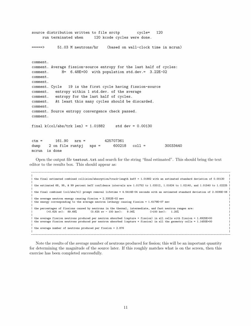
source distribution written to file srctp cycle= 120run terminated when 120 kcode cycles were done.

=====> 51.03 M neutrons/hr (based on wall-clock time in mcrun)

comment.comment. Average fission-source entropy for the last half of cycles:comment. H= 6.48E+00 with population std.dev.= 3.22E-02comment.comment.comment. Cycle 19 is the first cycle having fission-sourcecomment. entropy within 1 std.dev. of the averagecomment. entropy for the last half of cycles.comment. At least this many cycles should be discarded.comment.comment. Source entropy convergence check passed.comment.

final k(col/abs/trk len) = 1.01882 std dev = 0.00130

ctm = 161.90 nrn = 425707361dump 2 on file runtpj nps = 600218 coll = 30033440mcrun is done

Open the output file testout.txt and search for the string “final estimated”. This should bring the texteditor to the results box. This should appear as:

-----------------------------------------------------------------------------------------------------------------------------------| || the final estimated combined collision/absorption/track-length keff = 1.01882 with an estimated standard deviation of 0.00130 || || the estimated 68, 95, & 99 percent keff confidence intervals are 1.01752 to 1.02012, 1.01624 to 1.02140, and 1.01540 to 1.02225 || || the final combined (col/abs/tl) prompt removal lifetime = 4.5414E-04 seconds with an estimated standard deviation of 2.0035E-06 || || the average neutron energy causing fission = 2.3352E-02 mev || the energy corresponding to the average neutron lethargy causing fission = 1.6179E-07 mev || || the percentages of fissions caused by neutrons in the thermal, intermediate, and fast neutron ranges are: || (<0.625 ev): 89.68% (0.625 ev - 100 kev): 9.06% (>100 kev): 1.25% || || the average fission neutrons produced per neutron absorbed (capture + fission) in all cells with fission = 1.6925E+00 || the average fission neutrons produced per neutron absorbed (capture + fission) in all the geometry cells = 1.1455E+00 || || the average number of neutrons produced per fission = 2.876 || |-----------------------------------------------------------------------------------------------------------------------------------

Note the results of the average number of neutrons produced for fission; this will be an important quantityfor determining the magnitude of the source later. If this roughly matches what is on the screen, then thisexercise has been completed successfully.

11

Accident Tank

Lab

yrin

th

North

Figure 1: Exercise 1: Schematic of the facility geometry.

1010

10

10

1111

11

12

99

10/14/12 14:16:12plutonium-nitrate solution tank in a room

probid = 10/14/12 14:15:22basis: YZ( 0.000000, 1.000000, 0.000000)( 0.000000, 0.000000, 1.000000)origin:( 0.00, 0.00, 0.00)extent = ( 150.00, 150.00)

Figure 2: Exercise 1: Axial view of the can of plutonium nitrate solution.

12

10

11


probid = 10/14/12 14:16:33basis: XY( 1.000000, 0.000000, 0.000000)( 0.000000, 1.000000, 0.000000)origin:( 0.00, 0.00, 10.00)extent = ( 150.00, 150.00)

Figure 3: Exercise 1: Radial view of the can of plutonium nitrate solution at z = 10 cm.

1011

20

20

20

20 20

2020

21

21

21

22

22

22

22

23 23 23

23

30

31

32 33

34 34

3636

40

40

40

99

99

99


probid = 10/14/12 14:19:15basis: XY( 1.000000, 0.000000, 0.000000)( 0.000000, 1.000000, 0.000000)origin:( 250.00, -850.00, 10.00)extent = ( 2000.00, 2000.00)

Figure 4: Exercise 1: Slice of the entire facility in the x-y plane at z = 10 cm

13

Exercise 2: Source Convergence and Results Plotting

Since the fission source is usually unknown prior to running the calculation, a guess must be provided andan iterative method must be employed to converge it before accruing tally results. Otherwise, the answerswill be biased. The number of iterations required depends on both the characteristics of the problem andhow close the source guess is to the true fission source.

MCNP6 has a diagnostic called the Shannon entropy that is useful for assessing source convergence.The Shannon entropy is a measure of the shape of a distribution – the more “spread out” the distribution,the higher its Shannon entropy. At the beginning of the calculation, a uniform, coarse mesh is placed overthe problem geometry. Each cycle, the fission source points are binned according to their locations and aquantity called the Shannon entropy of the fission source distribution is obtained. By observing trends inthe Shannon entropy, and observing its convergence, the convergence of the underlying fission source maybe inferred.

The most effective means of doing this is by visualizing a plot of the Shannon entropy as a function ofcycle. The Shannon entropy is printed both to the output file and the screen. In principle these results couldbe parsed, and placed into a spreadsheet or plotting tool of the user’s choice. Alternatively, MCNP has thecapability to plot k and the Shannon entropy as a function of cycle via the tally plotter. To do this, MCNPrequires a run-tape (runtpe). For the run in the previous exercise, this is called caas1run, and this shall beneeded now.

In the command prompt, type

mcnp6 r = caas1run z

The z option tells MCNP to invoke the tally plotter. Like with the geometry plotter, X11 must beenabled to use the tally plotter. The user should then find a command prompt where MCNP expects a tallyplot command. First, it may be instructive to plot k as a function of cycle. The collision estimate of k as afunction of cycle may be obtained by entering

kcode 1

into the command prompt. Gridlines may be added to the plot by typing

scales 2

This is displayed in Fig. 5. While the plot has a bit of statistical noise, the trend shows that convergencein k occurs at about 20 cycles. Unfortunately, convergence in k is not the same as convergence in the fissionsource, which is necessary for getting an accurate estimate. For this, the trend in the Shannon entropy needsto be observed. To get this from the tally plotter, type

kcode 6

Again, there is noise in the plot, but it appears to converge around 25 cycles. Figure 6 gives a plot ofShannon entropy as a function of cycle. Therefore, the user should modify the KCODE card to skip at least25 cycles, probably more to be conservative.

Based on this information, copy caas1.txt to caas2.txt and modify the KCODE card to skip 30 cycleswhile keeping the number of active cycles at 100. Also, increase the batch size from 5000 to 20000, since thenext exercise require a more resolved fission source. The KCODE card should now read

kcode 20000 1.0 30 130

Rerun the problem:

mcnp6 i = caas2.txt o = caas2out.txt r = caas2run

The file results on the screen are:

source distribution written to file srctp cycle= 130

14

run terminated when 130 kcode cycles were done.

=====> 104.59 M neutrons/hr (based on wall-clock time in mcrun)

comment.comment. Average fission-source entropy for the last half of cycles:comment. H= 8.19E+00 with population std.dev.= 1.45E-02comment.comment.comment. Cycle 19 is the first cycle having fission-sourcecomment. entropy within 1 std.dev. of the averagecomment. entropy for the last half of cycles.comment. At least this many cycles should be discarded.comment.comment. Source entropy convergence check passed.comment.

final k(col/abs/trk len) = 1.01723 std dev = 0.00063

This confirms that cycle convergence as well as the prediction of k; the results are within 2-σ of eachother. As a check, a plot of the Shannon entropy also confirms this.

15

0 20 40 60 80 100 120

keff cycle number

0.8

0.9

1.

1.1

1.2

1.3k (collision)

kcode data from file caas1run

mcnp 6

probid: 10/14/12 13:57:49

nps 600218

runtpe = caas1run

dump 2

kcode 1

Figure 5: Exercise 2: Cyclewise collision estimate of k.

0 20 40 60 80 100 120

keff cycle number

4.

4.5

5.

5.5

6.

6.5

7.

Entropy of source

kcode data from file caas1run

mcnp 6

probid: 10/14/12 13:57:49

nps 600218

runtpe = caas1run

dump 2

kcode 6

Figure 6: Exercise 2: Shannon entropy of the fission source of each cycle.

16

Exercise 3: Writing a Fission Source File

Until now, everything discussed should have been review for an experienced MCNP user in the field ofcriticality. This exercise connects a criticality calculation to the shielding-type calculations needed for CAAS.To obtain an accurate representation of the fission source for a CAAS calculation, a criticality calculation isused to generate the source; this was reviewed in previous exercises. The next step is to get MCNP to writethe source, represented as a set of x, y, z points with emission energies, to a file. This file is then read intoMCNP in a fixed-source calculation, and tally results for detectors are then obtained.

MCNP has a “surface-source write” capability. Originally, this capability was designed to record particlestate information as it crosses surfaces, and write that state to a file. Later, this was extended to writing thesource points of a criticality calculation, although the name of a “surface-source write” remains, even thoughit is a misnomer for this specific use of it. Unfortunately, this capability does not yet work in parallel, andtherefore the accelerations from threading cannot be used.

To tell MCNP to write a source file, the SSW card is used having the following format:

SSW CEL = C1 C2 ...

where the listing after CEL is a list of all fissionable cells in the problem. In this specific exercise, thereis only one fissionable cell, cell 100, so the modification to the input file is straightforward. Copy the filecaas2.txt from the previous exercise to a new file called caas3.txt and insert the appropriate SSW cardamong the data cards. This new card is

ssw cel = 100

This will now have MCNP write a file containing source points in the active cycles. The default file nameis wssa, but this can be changed by including

wssa = filename

on the command line.Before running the problem, one thing to consider is that the continuum of the fission source is being

approximated by a discrete set of points. It is possible to run multiple instances of these same particles withdifferent random number sequences, however, it is not possible to generate any new points subsequently.Therefore, it is important to ensure the fission source is adequately captured during the calculation. For thenew settings on the KCODE card, approximately 100 times 20000 particles will be written, or 2 million. For asmall critical configuration such as this, 2 million should be sufficient, but may not be for large reactor-typesystems.

For this problem, let the file name of the surface source file be caassrc. Run the new problem by typingin the command prompt

mcnp6 i = caas3.txt o = caas3out.txt r = caas3run wssa = caassrc

The following should appear on the screen:

surface-source file caassrc written with 2000601 tracks.

If this is so, then this exercise is complete.

17

Exercise 4: Using the Fission Source File in a Fixed-Source Calculation

To test that this file was written successfully, it must be read back in by MCNP in a fixed-source calculation.To get started, make a copy of caas3.txt to caas4.txt.

Going from a criticality calculation to a fixed-source calculation has a peculiarity in how fission must betreated. In the eigenvalue problem, the fission process was already accounted for. Therefore, in the fixed-source problem, fission must be ignored or treated as capture. As a practical point of view, this configurationis supercritical, so if this system were run in fixed-source mode, a divergent fission chain would eventuallyoccur and the simulation would never terminate – or at least not until it runs out of memory from storingall the state information of progeny.

To treat fission as capture the NONU card is available. All cells where NONU = 0, fission is turned off.There are two ways to specify this: (1) on the cell cards, or (2) as a list of numbers in the data cards wherethe order of entries corresponds to the order that the cells are listed. Because any changes in the ordering ofthe cell cards may have deleterious and unintended effects, it sometimes makes the most sense to list theseon the cell cards. So on each cell card, after the imp:n=1 append a nonu=0. This ensures fission is turnedoff everywhere.

Next the KCODE, KSRC, and SSW cards must be removed. The NPS card must be inserted to tell MCNP howmany particles to run. Note that the total weight used in the calculation is equal to the number of particleswritten to the surface-source file, regardless of the value of NPS, and the weight is modified accordingly.Correspondingly, the results should not scale with NPS. If NPS is equal to the number of particles, then theparticles are transported as in the file. If it is is less, then a fraction of the particles are skipped and theweight is readjusted. If it is greater, then some of the source particles are duplicated with lesser weight andrun with different random number sequences. In the latter case, the value of NPS reported (deceptively) atthe end of the calculation will match the number written to the surface-source file, even though numeroustrajectories have been simulated.

Next, MCNP must know to read the surface-source file. This is accomplished with the SSR card

SSR CEL = C1 C2 ... WGT = W

The entries after CEL denote which cells to accept from the file. It is possible with the surface-sourcewrite to record information about fissions in numerous cells, and then only transport the ones for individualor a specific group of cells during the surface-source read. In this case, only cell 100 is available, so theissue is irrelevant. The WGT entry is a modifier for the source weight, and is needed to scale the intensity ofthe source to get doses and detector responses correct. The entry here is typically the number of neutronsemitted in the criticality accident, which is determined from other means than MCNP. Often times, the dataavailable for this is the energy release, which can be used to find the total number of fissions in the event.This number of fissions must be multiplied by an estimate of the number of neutrons released per fission ν,which can be obtained from the results of the criticality calculation used to generate the surface-source file.While this is an approximation, it typically is a good one as fission ν is a weak function of incident neutronenergy below a few MeV, which are the typical energies that cause fission in criticality problems.

For this problem, suppose the energy release is used to determine the magnitude of this event to be1 × 1015 fissions. Given the magnitude of ν is about 2.9 for this system, the multiplicative factor for theweight is 2.9× 1015. The SSR card that needs to be inserted is

ssr cel = 100 wgt = 2.9e15

Next, MCNP needs to know the number of particles NPS to run. Suppose for this trial run, 100,000histories is desired. Add an appropriate NPS card to the input file

nps 1e5

MCNP expects to read a file called rssa to get the source. Like with the surface-source write, this canbe overridden on the command line by adding

rssa = filename

18

Because the source is located in a file called critsource, that is the argument for the command line.Next, run the problem by typing on the command prompt

mcnp6 i = caas4.txt o = caas4out.txt r = caas4run rssa = caassrc

If the problem runs to completion, then this exercise has been successfully completed. Note that the valueof NPS printed to the screen may differ from 1× 105 because MCNP sampled histories with a probability ofabout 1/20, the ratio of the specified NPS to the number of particles written to the surface-source file.

19

Exercise 5: Defining the Detector

Now that the neutron source is available, the next step is to transport the neutrons into some detectorvolume. First, copy caas4.txt to caas5.txt.

A detector must be defined. For simplicity, assume the detector is a sphere of polyethylene (density of0.92 g/cc) with a radius of 5 cm. Realistic detectors are going to be far more complicated, but this willsuffice for pedagogical purposes. Suppose a detector location is chosen to be in the northwest room, centeredon its east wall, and just touching the ceiling. The spherical surface SPH may be used to define this. Theform for the surface is

ID SPH X0 Y0 Z0 RAD

where X0 Y0 Z0 are the coordinates for the center of the sphere and RAD is its radius. For the sphere atthis position, add the following surface card,

41 sph -255 -300 295 5.0

A material card for polyethylene with the appropriate thermal scattering law is needed:

c polyethlyenem5 1001 2

6000 1mt5 poly

The corresponding cell card is

300 5 -9.2000e-1 -41 imp:n=1 nonu=0

Also, the cell card for the northwest room must be modified to account for the subtracted space:

200 3 4.8333e-5 -20 +41 imp:n=1 nonu=0

At this point, the user should plot the geometry to ensure the detector has been placed appropriately.Once the geometry is verified, the next step is to place the tally for the response. The response is the

energy deposited in the detector during the radiation event. This can be obtained using the energy-depositiontally or the F6 type. The format is

F6:n C1 C2 ...

Here n denotes the tally is for neutrons, and the C1 C2 ... are a list of cells for which the tally is to bemade. Since the cell number is 300, the tally definition is

f6:n 300

The units of the F6 tally are Mev/gram of the cell, which are usually inconvenient for working with.Rather, this can be transformed to Gy or J/kg by a tally multiplier or FM card

fm6 1.6022e-10

Now that the tally is present, the problem is ready to be run. In the command prompt type

mcnp6 i = caas5.txt o = caas5out.txt r = caas5run rssa = caassrc

and run the problem. Open the output file caas1out.txt in a text editor and search for the literal string1tally. Below are the results of the tally and its relative uncertainty:

1tally 6 nps = 100429tally type 6 track length estimate of heating.

20

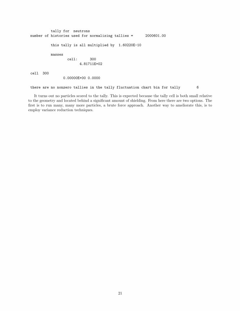
tally for neutronsnumber of histories used for normalizing tallies = 2000601.00

this tally is all multiplied by 1.60220E-10

massescell: 300

4.81711E+02

cell 3000.00000E+00 0.0000

there are no nonzero tallies in the tally fluctuation chart bin for tally 6

It turns out no particles scored to the tally. This is expected because the tally cell is both small relativeto the geometry and located behind a significant amount of shielding. From here there are two options. Thefirst is to run many, many more particles, a brute force approach. Another way to ameliorate this, is toemploy variance reduction techniques.

21

Exercise 6: Variance Reduction

Variance reduction techniques are a set of methods designed to increase the efficiency of the calculations. Allof the methods are mathematically proven to preserve the mean value of the tally – in other words, the answerafter a very large number of histories is the same. The variance reduction techniques each have parametersthat can be adjusted, and if these parameters are well chosen, then the calculation should converge morequickly. Conversely, it is also quite easy to pick parameters that actually decrease the efficiency. Therefore,there is a bit of judgment involved in deciding which parameters to employ and how to dial in the values ofthe specific parameters to improve performance.

One thing of note is that many of the institutional standards and guidelines actually prohibit the useof variance reduction techniques for design calculations. The presumption is that variance reduction toolsprovide an extra set of “knobs” that can be used to get misleading results and (more precisely) incorrectassessments of uncertainties. This issue arises because the relevant phase space of the problem is notadequately sampled, and therefore the results are failing to capture important pieces of information. This isnot a unique problem with variance reduction techniques, as any Monte Carlo calculation may be susceptibleto such biasing. Variance reduction techniques, however, can be abused in such a way to exacerbate thisissue. Therefore, users are advised to exercise caution and reasonable judgment in evaluating the quality ofanswers – codes should never be trusted as black boxes.

One diagnostic that MCNP offers are the statistical checks. There are ten checks performed on theconvergence trends and scoring behavior during the calculation. These look at what if any trends in theconvergence of the mean, relative uncertainty, variance of the variance (VOV), and the figure of merit (FOM)there may be. MCNP performs a check as to whether the trend matches expected behavior (e.g., the meanshould have no trend and vary randomly, the relative uncertainty should decrease as the square root of thenumber of histories, etc.). Also, relative uncertainty and the VOV – for VOV, think about having errorbars on the error bars of the results – are checked to ensure they are less than the canonical value of 0.1,above which results have a significant chance of being questionable. Finally, MCNP does a check on thescoring density function via the PDF slope, which checks to ensure enough very large, but rare contributionshave been sampled; this serves as a diagnostic for adequate sampling. Note that passing these tests doesnot guarantee the reliability of results (it is impossible to construct such a test), but it offers confidence.Ultimately, it is up to the user to determine whether the answers appear reasonable, and to use the statisticaltests as a guide for making that determination.

Variance reduction techniques usually try to achieve two competing goals. The first is to reduce theamount of variance incurred per history (i.e., reduce the spread in the scores), and the second is to reducethe amount of time per history. Usually doing the former harms the latter and vice versa. Therefore, pickingthe appropriate set of variance reduction parameters involves balancing these two considerations, and thereis some optimal set that maximizes efficiency. Thankfully, as a practical consideration, there seems to be afairly large range of parameters (a kind of mathematical plateau) that are nearly optimal. Therefore, oftenfor a fairly small amount of effort on the part of the user, nearly optimal variance reduction parameters canbe obtained. Furthermore, because gains are minimal once this plateau is found; the user needs to be carefulnot to invest too much time as there are diminishing returns (or even negative returns if more time is spenttweaking parameters than had that time just been invested in grinding out the calculation) past a certainpoint.

One important point about MCNP is that there are two variance reduction techniques on by default:implicit capture (also called survival biasing in other codes) and the weight cutoff (more accurately, a weightroulette game).

To understand implicit capture, it is first illustrative to understand how an analog Monte Carlo simulationwould occur. At a collision, suppose a neutron can either undergo scattering with probability p, or becaptured with probability 1− p. A random number is selected from zero to one, and if that number is lessthan p, the neutron scatters, continuing with a new energy and direction, otherwise, it disappears and thecode moves on to the next history.

In the non-analog case, each particle carries with it a statistical weight w that is multiplied by all tallyscores to preserve all means. In the analog case, the statistical weight is constant. With variance reductiongames, this weight changes throughout the history. For implicit capture, at a collision, rather than decidingwhether the neutron is absorbed or not, the neutron always scatters and has its weight multiplied by p. The

22

net effect of that this, in the long run, produces mathematically identical means, but because the historymay continue and therefore contribute more to tally scores each history, the variance tends to be lower eachhistory. This technique tends to decrease the amount of variance per history, but increases the amount oftime per history.

Because the weight can get arbitrarily low with implicit capture employed, allowing for a large amount oftime to be spent on histories that contribute little to tallies, there needs to be some mechanism to selectivelycull these tracks, but in a statistically fair way. This is the weight cutoff or weight roulette game. Whenthe weight w falls below a certain user-defined value, a roulette came is played. A random number fromzero to one is obtained, and if that number is greater than q, the particle is terminated. Otherwise, theparticle survives, but with its weight multiplied by 1/q, increasing the particle weight. The effect of thisis to remove many of the low-weight histories that contribute little to tallies from the simulation, but keepa certain fraction and weight their scores in a fair way to preserve mean values. Weight cutoff reduces theamount of time per history, but tends to increase the amount of variance. The hope is that the amount ofadditional variance incurred is more than compensated by the reduction in time per history.

These two techniques can be turned off or modified using either the CUT:N or PHYS:N cards. Sometimesit may be useful to try and change the parameters to get better performance, but the defaults are typicallysuitable for most applications.

For streaming problems of this sort, perhaps the most useful technique is also perhaps one of the mostdifficult to understand, the DXTRAN sphere. A DXTRAN sphere is an artificial spherical surface typicallycontaining a tally cell. At each collision and source emission, angular biasing is performed to pull particlestoward the sphere. The probability space is split or partitioned into two pieces: one where upon collision,the particle scatters directly toward the sphere, and streams without collision to the edge of the DXTRANsphere (the DXTRAN particle), and another where the particle continues as it would have with no DXTRANsphere (the non-DXTRAN particle). The DXTRAN particle has its weight reduced by the probabilitydensity of scattering in the direction toward the sphere along with the exponential attenuation throughany intervening materials from collision or source point to the edge of the sphere. This DXTRAN particle,from this point forward, ignores the DXTRAN game and transports normally. The non-DXTRAN particlecontinues, producing more DXTRAN particles at subsequent collisions, but with one minor modificationto keep the game fair. If the non-DXTRAN particle happens to reach the sphere during the course of itsnormal random walk, it is terminated, as that part of phase space within the sphere is no longer part of itsprobability space partition.

This technique, in effect, forces particles to a small region of space that they would be otherwise veryunlikely to go. Such is the case of the detector in this large facility model. The DXTRAN spheres are definedwith the DXT card:

DXT:n X1 Y1 Z1 RI1 RO1 X2 Y2 Z2 RI2 RO2 ... DWC1 DWC2

Here n is the particle type for neutrons (p for photons), X1 Y1 Z1 are the center of the first DXTRANsphere, RI1 RO1 are the inner and outer radii of the that sphere, subsequent DXTRAN spheres can bedefined similarly, and DWC1 DWC2 are upper and lower weight cutoff parameters. The inner and outer radiiof the spheres is a way to further refine the angular biasing toward the inner sphere; scattering toward theinner sphere is five times as likely as scattering to the outer sphere. Unless there is a compelling reason tothe contrary, it is typically best to pick the inner and outer radii as the same. The weight cutoff or roulettingparameters at the end of the list of spheres are important for ensuring that time is not spent on particleswith very low weight. If a particle is below DWC2, then the weight cutoff game is played to bring the weightof the particle back to be above DWC1.

To get started, copy the file caas5.txt to caas6a.txt. For this problem, the DXTRAN sphere shouldcover the detector region, the inner and outer radii being the same, with DWC1 and DWC2 being 5× 10−6 and1× 10−6 respectively. This card is

dxt:n -255 -300 295 5.0 5.0 5e-6 1e-6

One other consideration that arises with DXTRAN spheres and sources is that the probability of beingemitted in the direction of the DXTRAN sphere must be known. Recall that only the direction change incollisions matters (there is no incident directional dependence in MCNP), therefore it is appropriate to speak

23

of the probability of scattering cosines −1 ≤ µ ≤ 1 and the units of the probability density are per unitcosine. The PSC parameter must be added to the SSR card to provide this information. Since the sourceis from fission, which is isotropic, the probability of scattering is 1/2 everywhere (the total cosine range isnormalized to 2). The surface-source read card is now

ssr cel = 100 wgt = 2.9e15 psc = 0.5

Run the problem and analyze the output:

mcnp6 i = caas6a.txt o = caas6aout.txt r = caas6arun rssa = caassrc

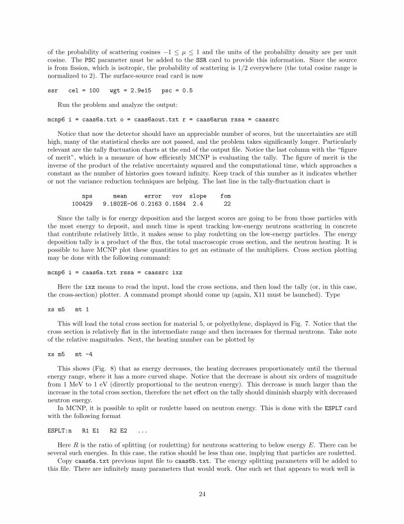
Notice that now the detector should have an appreciable number of scores, but the uncertainties are stillhigh, many of the statistical checks are not passed, and the problem takes significantly longer. Particularlyrelevant are the tally fluctuation charts at the end of the output file. Notice the last column with the “figureof merit”, which is a measure of how efficiently MCNP is evaluating the tally. The figure of merit is theinverse of the product of the relative uncertainty squared and the computational time, which approaches aconstant as the number of histories goes toward infinity. Keep track of this number as it indicates whetheror not the variance reduction techniques are helping. The last line in the tally-fluctuation chart is

nps mean error vov slope fom100429 9.1802E-06 0.2163 0.1584 2.4 22

Since the tally is for energy deposition and the largest scores are going to be from those particles withthe most energy to deposit, and much time is spent tracking low-energy neutrons scattering in concretethat contribute relatively little, it makes sense to play rouletting on the low-energy particles. The energydeposition tally is a product of the flux, the total macroscopic cross section, and the neutron heating. It ispossible to have MCNP plot these quantities to get an estimate of the multipliers. Cross section plottingmay be done with the following command:

mcnp6 i = caas6a.txt rssa = caassrc ixz

Here the ixz means to read the input, load the cross sections, and then load the tally (or, in this case,the cross-section) plotter. A command prompt should come up (again, X11 must be launched). Type

xs m5 mt 1

This will load the total cross section for material 5, or polyethylene, displayed in Fig. 7. Notice that thecross section is relatively flat in the intermediate range and then increases for thermal neutrons. Take noteof the relative magnitudes. Next, the heating number can be plotted by

xs m5 mt -4

This shows (Fig. 8) that as energy decreases, the heating decreases proportionately until the thermalenergy range, where it has a more curved shape. Notice that the decrease is about six orders of magnitudefrom 1 MeV to 1 eV (directly proportional to the neutron energy). This decrease is much larger than theincrease in the total cross section, therefore the net effect on the tally should diminish sharply with decreasedneutron energy.

In MCNP, it is possible to split or roulette based on neutron energy. This is done with the ESPLT cardwith the following format

ESPLT:n R1 E1 R2 E2 ...

Here R is the ratio of splitting (or rouletting) for neutrons scattering to below energy E. There can beseveral such energies. In this case, the ratios should be less than one, implying that particles are rouletted.

Copy caas6a.txt previous input file to caas6b.txt. The energy splitting parameters will be added tothis file. There are infinitely many parameters that would work. One such set that appears to work well is

24

esplt:n 0.25 1e-3 0.1 1e-6

This means that only a quarter of neutrons survive when scattering below 1 keV (with those survivinghaving their weight multiplied by four), and only a tenth survive when scattering below 1 eV (the survivalweight increased by a factor of ten).

Run the problem again:

mcnp6 i = caas6b.txt o = caas6bout.txt r = caas6brun rssa = caassrc

Notice that it runs much faster now. Also note that the figure of merit in the output file has increased.The relatively uncertainty may have increased slightly, as expected since there are fewer histories contributingto the tally, but this appears to be offset with the reduction in time per history. The last lines of the previousand current tally-fluctuation charts are

nps mean error vov slope fom100429 9.1802E-06 0.2163 0.1584 2.4 22100429 8.4930E-06 0.2363 0.2744 3.0 61

Next, in the output file search for the literal string 1dxtran. Below is information related to informationon neutrons going toward the DXTRAN spheres. The first block of information is the distribution of weights.

cumulative weight cumulativefraction of transmitted fraction of

times average weight transmissions transmissions per history total weight

1.0000E-01 572 0.21941 2.01416E+05 0.000371.0000E+00 512 0.41580 5.80285E+05 0.001442.0000E+00 115 0.45992 6.86117E+05 0.002705.0000E+00 140 0.51362 1.91980E+06 0.006231.0000E+01 141 0.56770 4.95372E+06 0.015341.0000E+02 359 0.70541 5.76020E+07 0.121281.0000E+03 128 0.75451 1.66081E+08 0.426741.0000E+38 36 0.76832 3.11690E+08 1.00000

Notice that a vast majority of the weight contributing to the DXTRAN sphere are a few particles withrelative weight that is very high. Below this is information where particles are coming from and reachingthe DXTRAN sphere. This is broken into hits and misses.

cell misses hits weight per history weight per hit

1 100 935976 508 5.12376E+04 2.01784E+082 101 227 0 0.00000E+00 0.00000E+003 102 49056 101 2.34447E+04 4.64392E+084 200 0 21 1.05844E+08 1.00834E+135 201 3333 41 2.29512E+04 1.11991E+0918 900 780108 1936 4.37772E+08 4.52380E+11

Notice that there seem to be very few tracks to the DXTRAN relatively, even in the room with thedetector itself (cell 200). The weight per hit also seems significantly higher than those coming from othercells (1 × 1013 versus contributions four to five orders of magnitude lower, on average). Note that becauseof the energy dependence of the heating value and total cross section, an unusually large weight to theDXTRAN sphere (the results of this table are energy independent) does not necessarily imply an unusuallylarge score to the tally, which is the real issue. Nonetheless, in this specific case, using DXTRAN hits isindeed an appropriate proxy for the tally scores. This information, along with the results of the previoussection of the table, implies that a few collisions are contributing a vast majority to the overall score ofthe tally. Considering their rarity (21 hits out of just over 1 × 105 histories) and high weight per history,

25

indicating their high importance to the tally result, it is advisable to increase the frequency of these events.This is possible using a technique called forced collisions.

When a collision is forced, MCNP decomposes the particle track into an uncollided and a collided part.The uncollided part immediately streams to the end of the cell and transport continues. The collided partundergoes a collision somewhere along its trajectory. The weight is partitioned according to the probabilityof colliding to preserve the mean value.

Forced collisions are controlled by the FCL:n card, which is a listing of numbers for each cell similar toNONU. Also like with NONU, FCL:n can be placed on the cell cards. The numbers can range from -1 to 1. Forhere, let the numbers be either 0 for not forcing collisions, or 1 meaning to always force them.

Copy caas6b.txt to caas6c.txt. On the cell cards, insert

fcl:n=k

where k is 1 for cells 101, 200, 201, 206, and 208 and 0 elsewhere. This particular list of cells are all thosein air that have a probable chance of contributing significantly to the DXTRAN sphere.

Run the problem again, and examine the tally-fluctuation charts in the output file:

mcnp6 i = caas6c.txt o = caas6cout.txt r = caas6crun rssa = caassrc

The previous and current are

nps mean error vov slope fom100429 8.4930E-06 0.2363 0.2744 3.0 61100429 7.8835E-05 0.7308 0.9728 1.8 5.7E+00

At first glance, it would appear that just based on the figure of merit alone, that forced collisions hasactually made the performance worse. This would be an incorrect conclusion, however. While the figure ofmerit has fallen by over a factor of ten and the error has dramatically increased, notice that the mean valueis over a factor of ten higher. The reason for this is that collisions near the detector tend to contribute thegreatest scores, and the previous calculations did not capture enough of them to have a reliable estimate ofthe mean. In other words, the tally-fluctuation chart values from the previous runs are deceptive in that theyare missing necessary portions of information. This is an example where examining the diagnostic tables(in this case, the DXTRAN contribution table) is important for getting correct answers. Had this problembeen run out longer without forced collisions, eventually large scores would have been made that would havesignificantly perturbed the mean and statistical quantities, serving as a clear warning signal. This may,however, have taken a long time to have arisen, and apparently reliable but wrong answers (too low by afactor of about six it turns out) may have been obtained.

Observe how the DXTRAN table changes:





1 100 937181 327 5.17773E+04 3.16776E+08

26

2 101 22244 36 4.28249E+00 2.37987E+053 102 49084 73 1.92037E+04 5.26286E+084 200 15 500 1.33771E+08 5.35243E+115 201 61724 143 3.42945E+04 4.79788E+0818 900 857400 3014 9.93944E+08 6.59749E+11

Notice that there are now significantly more particles (500 versus 21) are contributing to the DXTRANsphere from cell 200, the room with the detector. The weight per hit has also decreased to be closer to thosefrom elsewhere, which is desirable because the goal is to minimize the disparity in weight. This stronglysupports undersampling of important tracks is the reason for the dramatic increase in the mean.

Still, however, most of the scores to the DXTRAN are for particles with very high relative weight (about20% have a thousand times or more weight than average). The next step is to control this with weightwindows.

The weight-window game is a means to keep particle weights constrained to within a defined range. Thereare lower and upper weight-window bounds, which can be a function of space and energy. When a particlein a particular region of phase space has a weight above the upper weight-window bound, it is split to makeit within the weight window. Conversely, if the particle weight is below the lower weight-window bound,then it is rouletted such that the surviving particles have weights within the weight window. If the particleweight is already within the window, no action is taken.

Copy caas6c.txt to caas6d.txt. This file will serve as the starting point for developing the neededweight windows.

Weight windows can be used in conjunction with both cells and a superimposed mesh – the latter is moreversatile, and therefore the usual method of choice. Almost always, the weight-window mesh should coverthe entire geometry. The mesh is defined with the MESH card with a set of keywords. The mesh may be eitherin Cartesian, cylindrical, or spherical coordinates, and this is specified with the GEOM keyword. Here onlythe Cartesian or GEOM = XYZ case will be used. The x, y, z coordinates of lower corner of the mesh must bedefined with the ORIGIN keyword. Also, a reference x, y, z point must be defined with the REF keyword. Thereference point tells MCNP which mesh element to serve as the one for normalization and is typically onethat contains source particles. Next, a coarse mesh must be defined in x, y, z using the IMESH, JMESH, KMESHkeywords. The entries are absolute coordinates to define planes forming the mesh regions. Each coarse-meshelement may be further subdivided into some number of equally sized bins specified with the correspondingIINTS, JINTS, KINTS keywords. The example of this used in this exercise is

mesh geom = xyz origin = -1300 -1900 -50 ref = 0 0 5imesh = -1250 -260 -250 -200 800 850 1850 1900iints = 1 1 4 5 4 1 1 1jmesh = -1850 -850 -800 -305 -295 200 250jints = 1 1 1 2 1 2 1kmesh = 0 290 300 310kints = 1 3 1 1

The lower corner of the mesh corresponds to the lower corner of the geometry, or x = −1300 cm,y = −1900 cm, z = −50 cm. The reference point is located inside the can of plutonium nitrate solution,in line with keeping the weight-window values with respect to a source region. The mesh has eight coarseintervals with x bounds defined with the IMESH keyword. Each of these is subdivided into equally-sizedintervals with the IINTS keyword, with more resolution in the regions between the source and detector andlittle resolution faraway, where few neutrons are expected to contribute. This same idea is followed for the yand z coordinates. It may be a good idea at this point to pause to understand how the superimposed meshcorresponds with the geometry and understand why the particular choices were made. Note that this is notthe only valid choice for the mesh intervals, and almost surely not the optimal ones, but they appear to besufficient for the upcoming analysis.

A lower-weight window bound must be specified for each mesh element – the upper weight-window boundsin MCNP are determined by a global multiplicative constant (typically five, but this can be changed withthe WWP card). Because the number required is usually quite large, it is unreasonable to expect a user tounderstand the physics of the problem well enough to take intelligent guesses as to what those should be.

27

MCNP does provide, however, a weight-window generator, which can, using statistical methods, estimatewhat the lower weight-window bounds should be.

A note with using the weight-window generator with a mesh is that the mesh resolution needs to beappropriate. First, the mesh needs to be fine enough to capture the needed gradients in importance betweenregions; having too coarse a mesh may actually cause biasing so severe that performance is lower than analog.Conversely, because Monte Carlo techniques are used to estimate the lower weight-window bounds in eachelement, the tallies for each need to adequately sampled to have meaningful weight-window bounds. Goingtoo fine will mean that it will be too difficult for MCNP to find statistically resolved values, and either agreater amount of time would be needed to find parameters than simply “brute forcing” the desired result,or the results will be so erratic because of statistical noise to be useful. The previously chosen mesh tookthese issues into consideration, and the mesh resolution appears to appropriately balance them.

The weight-window generator is designed to optimize lower weight-window bounds for a specific tally. Itis invoked with the WWG card with the first entry being the index of the tally to attempt the optimizationfor. Other options of the weight-window generator card can be found in the MCNP Manual. In this case,the following card is needed

wwg 6

When MCNP is run, it will automatically create new tallies for each mesh element defined by the MESHcard and compute estimates of what the lower weight-window bounds should be. These will be printedout to a specially formatted file with the default name of wwout. This file may then be used as an input insubsequent runs. The weight-window generator may also be run iteratively using a previously obtained set ofweight-window bounds in the hope of obtaining a more statistically resolved set. Typically, a few iterationswill need to be performed before suitable weight-window bounds can be obtained.

Now run the problem:

mcnp6 i = caas6d.txt o = caas6dout.txt r = caas6drun rssa = caassrc

Note that the problem is now taking slightly longer. This is because MCNP is performing internalaccounting to produce estimates of the weight-window bounds. The results in the output file should nothave changed, because no new biasing parameters were introduced. The figure of merit, however, will likelybe lower because of the computational penalty incurred by the weight-window generator.

As previously mentioned, MCNP produces a file called wwout that contains these estimates. Rename thisfile to wwinp1, as it will be the first in a series of weight window input files. Also copy the MCNP input filecaas6d.txt to caas6e.txt.

To use the new weight-window file, the WWP:n card must be added. Specifically, the fifth parameter mustbe set to -1 to indicate that the weight-window bounds are to be obtained from a file. Add the followingcard to the MCNP input file

wwp:n 4j -1

Recall that the 4j means to “jump” over the first four entries, using their defaults. The fifth entry, theparameter to tell where MCNP should obtain the weight-window bounds, is then changed to -1. A fulldescription of the WWP card may be obtained in the MCNP Manual.

Which file to use is done on the execution command line. This is done with the wwinp = <file> option,where <file> is the name of the weight-window file, or wwinp1 in this case. Run the problem:

mcnp6 i = caas6e.txt o = caas6eout.txt r = caas6erun rssa = caassrc wwinp = wwinp1

MCNP is now using the previously obtained set of weight-window bounds to obtain a new, and hopefullyimproved set. Because of the new biasing games being played, this run takes significantly longer than before.Upon completion, a new file called wwout is produced containing the new set of parameters; rename this fileto wwinp2.

Examining the new output file should show that uncertainty is significantly reduced. The last lines inthe two different tally-fluctuation charts are

28

nps mean error vov slope fom100429 7.8835E-05 0.7308 0.9728 1.8 5.5E+00100429 4.9018E-05 0.2293 0.3095 1.8 3.2E+00

The DXTRAN tables are also informative:





1 100 9981049 1973 7.51494E+04 7.62007E+072 101 314745 411 1.23567E+00 6.01482E+033 102 528737 378 3.17756E+04 1.68176E+084 200 660873 25635 1.67741E+08 1.30908E+105 201 882385 1316 4.21140E+04 6.40223E+0718 900 23405644 170079 1.42156E+09 1.67215E+10

The introduction of weight control has largely reduced the number of extremely high weight contributions.Less than 1% of the transmissions to the DXTRAN sphere have a weight a factor of a thousand greater thanaverage. The number of contributions from cell 200 has also increased dramatically, going from 500 to over25000. Consequently, the weight per hit is also a factor of 40 lower and nearer the weight per hit from othernearby regions of the problem (namely cell 900, which accounts for neutrons going from the accident throughthe concrete wall).

It is desirable to iterate again to further improve the weight windows. First, copy caas6e.txt file tocaas6f.txt. Also, increasing the number of histories run will get more reliable estimates of the lower weight-window bounds. There is a particular subtlety with doing this with a surface source, however. The averagesource weight is related to the number of histories run (the NPS) and the number of tracks stored in thesurface-source file. While results of tallies are independent of the NPS chosen, the weight windows are not,and things need to adjusted accordingly.

Doubling NPS means that the average source weight is reduced by half. The weight windows, however,are expecting the same average source weight. This can be done if the emitted weight on the SSR card isdoubled along with NPS:

nps 2e5ssr cel = 100 wgt = 5.8e15 psc = 0.5

Tally scores, however, will be a factor of two too high. This can be fixed by adjusting the halving thetally multiplier:

fm6 8.0110e-11

Remember that none of this is needed in a normal, fixed-source (SDEF) problem.Run the problem again, but with the new set of weight windows

mcnp6 i = caas6f.txt o = caas6fout.txt r = caas6frun rssa = caassrc wwinp = wwinp2

29

The tally fluctuation charts show markedly improved performance. The last lines of the previous andcurrent runs are

nps mean error vov slope fom100429 4.9018E-05 0.2293 0.3095 1.8 3.2E+00199653 5.5539E-05 0.0692 0.0331 3.8 14

The entire tally fluctuation chart is

nps mean error vov slope fom16000 7.5688E-05 0.2425 0.3509 1.7 1432000 6.7599E-05 0.1631 0.1884 1.9 1648000 6.4932E-05 0.1262 0.1265 1.9 1864000 6.0339E-05 0.1094 0.1000 2.1 1880000 6.0882E-05 0.0985 0.0718 2.4 1896000 5.9743E-05 0.0949 0.0633 2.5 16112000 5.7343E-05 0.0948 0.0643 2.4 14128000 5.6485E-05 0.0876 0.0566 2.9 14144000 5.6947E-05 0.0826 0.0482 2.9 14160000 5.6425E-05 0.0773 0.0435 3.1 14176000 5.6144E-05 0.0740 0.0384 3.2 14192000 5.5828E-05 0.0710 0.0341 3.6 14199653 5.5539E-05 0.0692 0.0331 3.8 14

The relative uncertainty is less than 10% and all statistical checks have been passed. The figure of merit isalso significantly higher, indicating that weight windows have improved the efficiency of getting the answers,as well as their reliability. As a check, the mean is also about the same as before, and no significant jumpsare observed. Also, the slope of the PDF tail is significantly greater (now being above three) and steadilyimproving. The reason this matters is that the tail of the PDF slope is related to those rare extremely highweight contributions. As the magnitude of the score gets very large, the frequency of that score occurringshould decrease rapidly. Having a low PDF slope indicates that the tail has not been adequately resolved. Inother words, there are likely some extremely high weight contributions that have not been sampled enough.

As an aside, the reason for the choice of a PDF slope of three for the statistical check criteria is that thisis the minimum requirement for the central limit theorem being satisfied. If this condition is met, both themean and standard deviation (uncertainty) exist, and the relative uncertainty should decrease as the squareroot of the number of histories. If this behavior is expected (which it always is in cases of interest exceptfor a notable exception involving F5 tallies), then the true PDF slope must fall off with at least a slope ofthree, and resolving that behavior is an indicator of reliability.

In principle this calculation is finished. The tally means appear reasonable and all statistical checks arepassed. Once in a while, it is good to verify that things are well behaved with an even longer run. Asan exercise, run the problem with one million histories, remembering to adjust the source weight and tallymultiplier.

The tally-fluctuation chart of the longer run confirm what was seen in the previous case:

nps mean error vov slope fom64000 6.0176E-05 0.1330 0.1304 1.8 12128000 5.5487E-05 0.0918 0.0692 2.6 13192000 5.2667E-05 0.0781 0.0522 2.5 12256000 5.1279E-05 0.0689 0.0557 3.2 12320000 5.1672E-05 0.0677 0.0527 3.1 9.9E+00384000 5.1803E-05 0.0597 0.0428 3.5 11448000 5.0410E-05 0.0544 0.0378 3.8 11512000 5.0908E-05 0.0498 0.0311 4.1 12576000 4.9349E-05 0.0465 0.0290 4.2 12640000 4.9371E-05 0.0435 0.0252 4.5 12

30

704000 5.0017E-05 0.0415 0.0217 4.5 12768000 5.0807E-05 0.0398 0.0192 4.3 12832000 5.1213E-05 0.0380 0.0174 4.0 12896000 5.1107E-05 0.0363 0.0158 4.2 12960000 5.1281E-05 0.0350 0.0145 4.5 121000571 5.0766E-05 0.0341 0.0142 4.6 13

It turns out that with application of variance reduction techniques (DXTRAN, energy cutoffs, forcedcollisions, and weight windows), this problem is quite easy to solve. Getting results for detectors furtheraway is more difficult, and will require better attention to variance reduction parameters including the weight-window mesh resolution, and probably just running more histories. The variance reduction techniques justdiscussed, however, should mostly be sufficient to solve this type of problem.

31

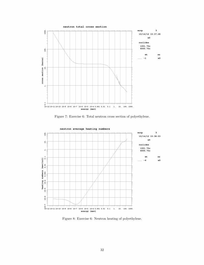
10-12 10-11 10-10 10-9 10-8 10-7 10-6 10-5 10-4 0.001 0.01 0.1 1. 10. 100. 1000.

energy (mev)

0.1

1.

10.

100.

1000.

cross section (barns)

cross section plot

neutron total cross section

mcnp 5

10/14/12 15:37:28

m5

nuclides

1001.70c 6000.70c

mt xs

-1 m5

.

Figure 7: Exercise 6: Total neutron cross section of polyethylene.

10-12 10-11 10-10 10-9 10-8 10-7 10-6 10-5 10-4 0.001 0.01 0.1 1. 10. 100. 1000.

energy (mev)

10-7

10-6

10-5

10-4

0.001

0.01

0.1

1.

10.

100.

heating numbers (mev/col)

cross section plot

neutron average heating numbers

mcnp 5

10/14/12 15:38:03

m5

nuclides

1001.70c 6000.70c

mt xs

-4 m5

.

Figure 8: Exercise 6: Neutron heating of polyethylene.

32

Exercise 7: Facility Doses to Personnel

In addition to the alarm system design, another consideration is estimating the doses delivered to personnel asa consequence of a criticality accident. These can be important for the development of evacuation proceduresand emergency response activities. MCNP6 can compute flux or dose maps on a spatially resolved mesh.This exercise details how to set up a flux mesh and how to apply dose response functions D(E) to get theenergy absorbed by tissue.

For now, these exercises have focused explicitly on neutrons only. For dose calculations, neutrons willlikely contribute most of the dose, but gamma doses may not be negligible. Since gammas are also generatedfrom fission, this means that the surface-source file will need to be regenerated.

Copy the file caas3.txt to caas7a.txt. To add photons to the eigenvalue calculation, the MODE cardmust be used. The format is the card name followed by a list of characters denoting the particle types tobe used. The default is neutrons only, for which the symbol is n. The symbol for gammas or photons is p.Insert the following card into the new file:

mode n p

The surface-source write or SSW card does not need to be changed. There is an optional argument calledPTY, which can be used to list the particle types that need to be recorded. The default is to record everything.To be explicit, the following could be used but is not necessary:

ssw cel = 100 pty = n p

Run the problem with the surface-source file name of caas7src:

mcnp6 i = caas7a.txt o = caas7aout.txt r = caas7arun wssa = caas7src

The problem should take longer than before because MCNP is tracking photons during the active cycles.At the end of the problem, the following line should appear on the screen:

surface-source file caas7src written with 3798013 tracks.

About 3.8 million tracks have been written to the file, up from the about 2 million neutron histories run.This is because the fission gammas produced are also stored in the file in addition to the neutrons.

Next, copy the file caas4.txt to caas7b.txt. Modify the MODE card to include photons. Note that thisfile should contain the nonu=0 on the cell cards, which must be changed to nonu=2 This implies that neitherfission neutrons nor fission gammas will not be produced, as they are already encountered in the source.Photons produced from neutron capture or inelastic scattering are still emitted, however.

Run this problem with 1× 105 histories:

mcnp6 i = caas7b.txt o = caas7bout.txt r = caas7brun rssa = caas7src

Examine the neutron and photon creation tables in the output file:

neutron creation tracks weight energy neutron loss tracks weight energy(per source particle) (per source particle)

source 100433 2.9105E+15 2.1048E+00 escape 13615 3.1943E+14 7.5768E-02nucl. interaction 0 0. 0. energy cutoff 0 0. 0.particle decay 0 0. 0. time cutoff 0 0. 0.weight window 0 0. 0. weight window 0 0. 0.cell importance 0 0. 0. cell importance 0 0. 0.weight cutoff 0 1.8468E+14 2.4325E-07 weight cutoff 86821 1.8577E+14 8.6359E-05e or t importance 0 0. 0. e or t importance 0 0. 0.dxtran 0 0. 0. dxtran 0 0. 0.forced collisions 0 0. 0. forced collisions 0 0. 0.exp. transform 0 0. 0. exp. transform 0 0. 0.upscattering 0 0. 1.2348E-07 downscattering 0 0. 1.9664E+00photonuclear 0 0. 0. capture 0 1.5555E+15 5.4491E-02(n,xn) 6 1.2898E+11 4.0087E-05 loss to (n,xn) 3 6.4492E+10 2.1743E-04prompt fission 0 0. 0. loss to fission 0 1.0345E+15 7.8795E-03delayed fission 0 0. 0. nucl. interaction 0 0. 0.prompt photofis 0 0. 0. particle decay 0 0. 0.

33

tabular boundary 0 0. 0. tabular boundary 0 0. 0.tabular sampling 0 0. 0. elastic scatter 0 0. 0.

total 100439 3.0953E+15 2.1048E+00 total 100439 3.0953E+15 2.1048E+00

number of neutrons banked 3 average time of (shakes) cutoffsneutron tracks per source particle 5.0186E-02 escape 5.7382E+04 tco 1.0000E+33neutron collisions per source particle 2.9970E+00 capture 7.3138E+04 eco 0.0000E+00total neutron collisions 5997993 capture or escape 7.0453E+04 wc1 -5.0000E-01net multiplication 1.0000E+00 0.0000 any termination 5.7821E+04 wc2 -2.5000E-01

photon creation tracks weight energy photon loss tracks weight energy(per source particle) (per source particle)

source 89997 7.9409E+15 8.6851E-01 escape 12702 7.1632E+14 1.0556E-01nucl. interaction 0 0. 0. energy cutoff 0 0. 8.3789E-05particle decay 0 0. 0. time cutoff 0 0. 0.weight window 0 0. 0. weight window 0 0. 0.cell importance 0 0. 0. cell importance 0 0. 0.weight cutoff 0 0. 0. weight cutoff 0 0. 0.e or t importance 0 0. 0. e or t importance 0 0. 0.dxtran 0 0. 0. dxtran 0 0. 0.forced collisions 0 0. 0. forced collisions 0 0. 0.exp. transform 0 0. 0. exp. transform 0 0. 0.from neutrons 93800 4.3477E+15 1.2200E+00 compton scatter 0 0. 1.6561E+00bremsstrahlung 56944 2.9505E+15 2.5418E-02 capture 331099 2.2237E+16 2.8010E-01p-annihilation 12824 5.4425E+14 3.5023E-02 pair production 6412 2.7212E+14 1.5504E-01photonuclear 0 0. 0. photonuclear abs 0 0. 0.electron x-rays 0 0. 0. loss to photofis 0 0. 0.compton fluores 0 0. 0.muon capt fluores 0 0. 0.1st fluorescence 83196 6.3204E+15 4.5743E-022nd fluorescence 13452 1.1218E+15 2.2097E-03(gamma,xgamma) 0 0. 0.tabular sampling 0 0. 0.prompt photofis 0 0. 0.

total 350213 2.3226E+16 2.1969E+00 total 350213 2.3226E+16 2.1969E+00

number of photons banked 267017 average time of (shakes) cutoffsphoton tracks per source particle 1.7499E-01 escape 4.3518E+04 tco 1.0000E+33photon collisions per source particle 7.3072E-01 capture 1.5038E+04 eco 1.0000E-03total photon collisions 1462411 capture or escape 1.5927E+04 wc1 -5.0000E-01

any termination 1.6459E+04 wc2 -2.5000E-01

For each neutron emitted in the simulation, about 0.9 photons are emitted from the source. The weightof photon source particles, however, is about 2.73 times higher than neutron sources. This implies that about2.44 photons are emitted per neutron emitted from fission. Multiplying by about 2.9 neutrons per fission,this would imply that just over 7 photons are emitted per fission.

Additional photons are produced as secondaries from neutron collisions in this simulation, with manymore coming from other photon-electron induced physical processes (e.g., bresstrahlung). Note that MCNP6is not explicitly tracking electrons in this simulation – doing so would slow the simulation down by ordersof magnitude. To produce x-rays from bresstrahlung, MCNP6 uses the thick-target approximation, whichpreserves the mean number of bresstrahlung photons produced, but only at the point of the photoatomiccollision. Photonuclear effects (e.g., neutrons produced from high-energy photon collisions) are neglected. Itwould be possible to include this effect with the PHYS:P card, but they should be negligible for this type ofproblem.

Copy caas7b.txt to caas7c.txt. Next the neutron and photon mesh tallies will be added. First, it isimportant to decide the resolution of the mesh. For this, using a 50 cm × 50 cm mesh in the x− y directionextending from floor to ceiling seems appropriate.

The are done by way of the FMESH cards. The format is very similar to the MESH card, except that thereis no REF keyword needed. The following FMESH cards should be inserted:

c ### mesh talliesc neutron mesh tallyfmesh104:n geom = xyz origin = -1300 -1900 0

imesh = 1900 iints = 64jmesh = 250 jints = 43kmesh = 300 kints = 1

c photon mesh tally

34

fmesh204:p geom = xyz origin = -1300 -1900 0imesh = 1900 iints = 64jmesh = 250 jints = 43kmesh = 300 kints = 1

If this calculation is run, neutron and photon fluxes averaged over each mesh element will be produced.This is not, however, the answer that is desired. To get the dose (in Gy), dose functions need to appliedwith DE and DF cards. These specify energy-dependent tally multipliers that use either linear or logarithmicinterpolation. The cards are:

c ### fluence to dose (particles/cm^2 to Gy) kerma response factorsc neutronsc J. Shultis, R. Faw, "Radiation Shielding" p. 477c selected values from Table D.8 (use larger set for actual calculations)de104 log 2.00e-06 2.00e-05 2.00e-04 2.00e-03 2.00e-02 2.00e-01

1.00e+00 2.00e+00 3.03e+00 3.99e+00 5.02e+00 7.60e+001.00e+01 1.21e+01 1.45e+01 2.00e+01

df104 log 2.33e-14 9.32e-15 2.26e-14 2.01e-13 1.81e-12 9.88e-122.53e-11 3.03e-11 3.58e-11 4.10e-11 4.56e-11 5.25e-115.72e-11 6.14e-11 6.60e-11 7.35e-11

c photonsc ANSI/ANS-6.1.1 1977de204 log 1.00e-02 3.00e-02 5.00e-02 7.00e-02 1.00e-01 1.50e-01

2.00e-01 2.50e-01 3.00e-01 3.50e-01 4.00e-01 4.50e-015.00e-01 5.50e-01 6.00e-01 6.50e-01 7.00e-01 8.00e-011.00e+00 1.40e+00 1.80e+00 2.20e+00 2.60e+00 2.80e+003.25e+00 3.75e+00 4.25e+00 4.75e+00 5.00e+00 5.25e+005.75e+00 5.75e+00 6.25e+00 6.75e+00 7.50e+00 9.00e+001.10e+01 1.30e+01 1.30e+01 1.50e+01

df204 log 1.10e-11 1.62e-12 8.06e-13 7.17e-13 7.86e-13 1.05e-121.39e-12 1.75e-12 2.11e-12 2.44e-12 2.74e-12 3.00e-123.25e-12 3.53e-12 3.78e-12 4.00e-12 4.22e-12 4.67e-125.50e-12 6.97e-12 8.31e-12 9.50e-12 1.06e-11 1.11e-111.23e-11 1.34e-11 1.45e-11 1.56e-11 1.61e-11 1.67e-111.77e-11 1.87e-11 1.98e-11 2.13e-11 2.44e-11 2.86e-113.28e-11 3.69e-11

The mesh tally results will be printed to a text file with a default file name of meshtal. Like with otheroptions, this can be changed on the execution line. Run the problem

mcnp6 i = caas7c.txt o = caas7cout.txt r = caas7crun meshtal = caas7cmesh rssa = caas7src

Once the problem completes, it would be useful to visualize the results. This can be done in the tallyplotter. On the execute line, type

mcnp6 z r = caas7crun

MCNP6 will load the runtpe file. On the command prompt, type

fmesh 104

This will load the geometry plotter and display tally 104, the neutron mesh tally. Click on the windowto see the results. These are displayed in Fig. 9. It should be readily apparent that while the dose in theroom with the accident is well-resolved, the doses in the other rooms are not. The appearance of coloredstreaks are clear signs of poor sampling, and they are in abundance.

35

The plotter may also plot the relative uncertainties. Click on the box in bottom-left corner of thegeometry plotter and type fmrelerr. A plot of the relative uncertainty should appear. This is displayed inFig. 10. Note that except for the region immediately around the source, the relative uncertainties are veryhigh.

A plot of the photon tally may be brought up by clicking on the same box and typing fmesh 204. Thisbrings up the photon plot, which looks similar to the neutron one. The relative uncertainty may also belikewise plotted. After doing this, close the plotter.

At this point, the only real viable option currently in MCNP6 is to run many, many more particles.While some variance reduction techniques may be tried, there is currently no automatic way to generatevariance reduction parameters (e.g., weight windows) for a mesh tally. This is a topic of future research anddevelopment in MCNP6.

36

2.8-10

.66

6.2-8

.000014

.003



Mesh Tally 104nps 2001333runtpe = runtphdump 2

Figure 9: Exercise 7: Neutron dose (in Gy) mesh tally.

0

1

.05

.1

.15

.25

.5

1



Mesh Tally 104nps 2001333runtpe = runtphdump 2

Figure 10: Exercise 7: Relative uncertainties of neutron dose mesh tally.

37

References

[1] MCNP6 Development Team, “Initial MCNP6 Release Overview”, J. Nucl. Technol., Accepted forPublication, also LA-UR-11-07082, Los Alamos National Laboratory (2011).

[2] B.A. Greenfield, “Criticality Alarm System Design Guide with Accompanying Alarm System Devel-opment for the Radiochemical Processing Laboratory in Richland, Washington,” Pacific NorthwestNational Laboratory, PNNL-18348 (2009).

[3] X-5 Monte Carlo Team, “MCNP - A General N-Particle Transport Code, Version 5, Volume I: Overviewand Theory,” Los Alamos National Laboratory, LA-UR-03-1987 (2003).

[4] R. Brewer (Ed.), “Criticality Calculations with MCNP5: A Primer,” Los Alamos National Laboratory,LA-UR-09-00380 (2009).

[5] R.J. McConn, C.J. Gesh, R.T. Pagh, R.A. Rucker, R.G. Williams, “Compendium of Material Compo-sition Data for Radiation Transport Modeling, Revision 1,” PNNL-15870 Rev. 1 (2011).

38

coversheet - los alamos national laboratory: mcnp home … · mcnp6 for criticality accident alarm...

Documents