Covariate Adjusted Functional Principal Component Analysis

(FPCA) for Longitudinal Data

Ci-Ren Jiang & Jane-Ling WangUniversity of California, Davis

National Taiwan UniversityJuly 9, 2009

Ci-Ren JiangPh. D. Candidate, UC Davis

Outline

Introduction

(Univariate) Covariate adjusted FPCA

? (Multivariate ) Covariate adjusted FPCA

FPCA as a building block for Modeling

Application to PET data

1. Introduction

Principal Component analysis is a standard dimension reduction tool for multivariate data. It has been extended to functional data and termed functional principal component analysis (FPCA).

Standard FPCA approaches treat functional data as if they are from a single population.

Our goal is to accommodate covariate information in the framework of FPCA for longitudinal data.

Functional vs. Longitudinal Data

A sample of curves, with one curve, X(t), per subject.

- These curves are usually considered realizations of a stochastic process in . - dimensional

Functional Data - In reality, X(t) is recorded at a regular and dense time grid high-dimensional.

Longitudinal Data – irregularly sampled X(t).

- often sparse, as in medical follow-up studies.

2( )L I

Longitudinal AIDS Data

CD4 counts of 369 patients were recorded. The number , of repeated measurements for subject i, varies with an average of 6.44.

This resulted in longitudinal data of uneven no. of measurements at irregular time points.

in

CD4 Counts of First 25 Patients

-3 -2 -1 0 1 2 3 4 5 60

500

1000

1500

2000

2500

3000

3500

time since seroconversion

CD

4 C

ount

Review of FPCA² A ssume data originates from a random function X (t),

with mean ¹ (t) and covariance function

¡ (s; t) = C ov(X (s); X (t)), s & t 2 a compact interval.

² FP CA corresponds to a spectral decomposition of thecovariance ¡ (s; t), which leads to K arhunen-Loeve de-composition of the random function as:

X (t) = ¹ (t) +XXX

k

A kÁk(t);

where var(A k) = ¸ k and Ák(t) are the eigenvalues andeigenfunctions of ¡ (s; t);

A k =R

f X (t) ¡ ¹ (t)gÁ(t)dt are orthogoanl

Review of FPCA

Both longitudinal and functional data may be observed with noise (measurement errors).

the observed data for subject i might be

ij

1(t ) = ( ) ( ) ( ).ij ij i ijij i ik k

kYY t A t e t

Review of FPCA

Functional Data Dauxois, Pousse & Romain (1982) Rice & Silverman (1991) Cardot (2000) Hall & Hosseini-Nasab (2006)

Longitudinal Data Shi, Weiss & Taylor(1996) James, Sugar & Hastie(2000) Rice & Wu (2001) Yao, Müller & Wang (2005)

Steps to FPCA

1. Estimate the mean ¹ (t) and covariance ¡ (s; t).(T his usually involves smoothing).

2. Estimate the eigenvalues and eigenfunctions of ¡ (s; t).3. Estimate P C scores A i k =

RRR(X (t) ¡ ¹ (t))Á(t)dt.

² W hen functional data are observed at irregular & fewtime points, the functional P C scores cannot be esti-mated through integration method.

² Y ao et al. (2005) proposed PACE to resolve this issue.

A i k = E (A i k jY i ) = ^kÁT

k § ¡ 1Y i

(Y i ¡ ¹ i )

Estimation of Mean Function

Taipei 101

CD4 Counts of First 25 Patients

-3 -2 -1 0 1 2 3 4 5 60

500

1000

1500

2000

2500

3000

3500

time since seroconversion

CD

4 C

ount

CD4 Counts of First 25 Patients

-3 -2 -1 0 1 2 3 4 5 60

500

1000

1500

2000

2500

3000

3500

time since seroconversion

CD

4 C

ount

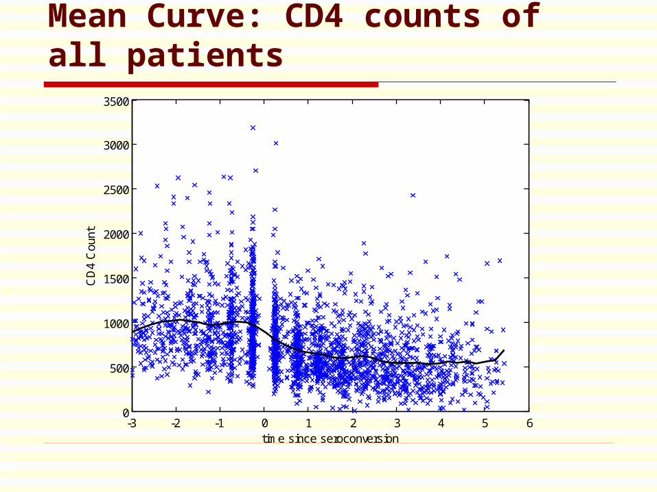
Mean Curve: CD4 counts of all patients

-3 -2 -1 0 1 2 3 4 5 60

500

1000

1500

2000

2500

3000

3500

time since seroconversion

CD

4 C

ount

Estimation of Covariance Function

Row Covariance Plot: [ ( ) ( )][ ( ) ( )], ,ij ij ik ikY t t Y t t j k

Y(t)= X(t)+e(t)

Cov (Y(s), Y(t))

= Cov (X(s), X(t)),

if s t,

2

var(Y(t))

=var(X(t))

b t

+

u

.

Row Covariance Plot: [ ( ) ( )][ ( ) ( )], ,ij ij ik ikY t t Y t t j k

Y(t)= X(t)+e(t)

Cov (Y(s), Y(t))

= Cov (X(s), X(t)),

if s t,

2

var(Y(t))

=var(X(t))

b t

+

u

.

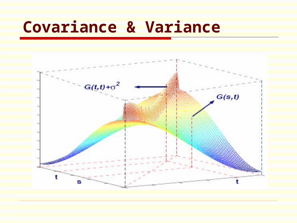
Covariance & Variance

References

Yao, Müller and Wang (2005, JASA)

Methods and theory for the mean and covariance functions.

Hall, Müller and Wang (2006, AOS)

Theory on eigenfunctions and eigenvalues.

End of Introduction

2. Covariate adjusted FPCA – Univariate Z

For dense functional data

Chiou, Müller & Wang (2003)

Cardot (2006)

Their method does not work for sparse dara.

We propose two ways:

fFPCA & mFPCA

Covariate adjusted FPCA: Longitudinal Data

Suppose the data originate froma random function X (t; z)

with mean ¹ (t; z)and covariance function ¡ (s; t; z),

where z is the value of a covariate Z ,and s and t are in a compact time interval.

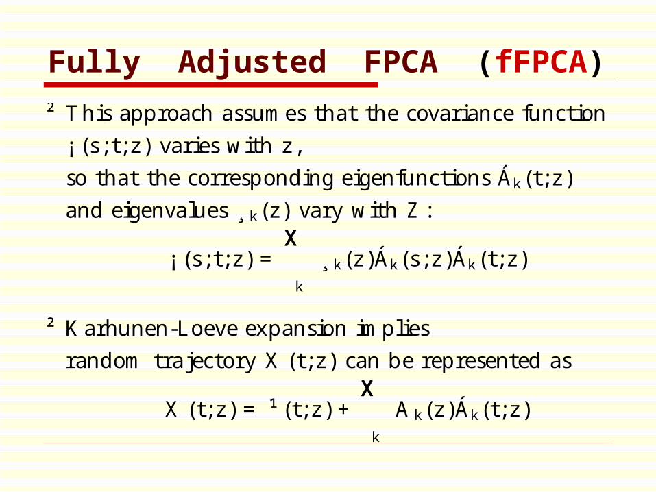
Fully Adjusted FPCA (fFPCA)

² T his approach assumes that the covariance function

¡ (s; t; z) varies with z,

so that the corresponding eigenfunctions Ák(t; z)

and eigenvalues ¸ k(z) vary with Z :

¡ (s; t; z) =XXX

k

¸ k(z)Ák(s; z)Ák(t; z)

² K arhunen-Loeve expansion implies

random trajectory X (t; z) can be represented as

X (t; z) = ¹ (t; z) +XXX

k

A k(z)Ák(t; z)

Mean Adjusted FPCA (mFPCA)

² T he second approach took the view that the covariateZ is a random variable, and if we pool all the subjectstogether after centering each individual curve to zero,we would have a pooled covariance function

¡ ¤(s; t) =XXX

k

¸ ¤kÁ¤

k(s)Á¤k(t)

² K arhunen-Loeve expansion thus implies that the ran-dom trajectory X (t; z) can be represented as

X (t; z) = ¹ (t; z) +XXX

k

A ¤kÁ¤

k(t)

Estimation: Mean Function

T he mean function for fFP CA and mFP CAare the same and can be estimated using anytwo-dimensional scatter-plot smoother ofY i j on (Ti j ; Z i ):

For examples:

Nadaraya-Watson kernel estimator:

¹ N W (t; z) =

P ni =1

P N ij =1 K 2( t¡ Ti j

h¹ ;t; z¡ Z i

h¹ ;z)Y i j

P ni =1

P N ij =1 K 2( t¡ Ti j

h¹ ;t; z¡ Z i

h¹ ;z)

Estimation: Mean Function

Local linear estimator:

¹ L (t; z) = ^0; where for ¯ = (¯ 0; ¯ 1; ¯ 2)

^= argmin¯

nXXX

i =1

N iXXX

j =1

K 2(t ¡ Ti j

h¹ ;t;

z ¡ Z i

h¹ ;z)

£ [Y i j ¡ ¯ 0 ¡ ¯ 1(Ti j ¡ t) ¡ ¯ 2(Z i ¡ z)]2:

CD4 Counts of All Patients and Mean Curve

-3 -2 -1 0 1 2 3 4 5 60

500

1000

1500

2000

2500

3000

3500

time since seroconversion

CD

4 C

ount

AIDS CD4: Estimated Mean

Estimation: Covariance Function

T he covariance estimators can also be expressedas a scatter-plot smoother of the so called\ raw covariances" de ned as:

C i j k = (Y i j ¡ ¹ (Ti j ; Z i ))(Y i k ¡ ¹ (Ti k; Z i )):

² fFP CA : three-dimensional smoother of

C i j k on (Ti j ; Ti k; Z i )

² mFP CA : two-dimensional smoother of

C i j k on (Ti j ; Ti k).

Estimation: Covariance Function

Since

cov(Y i j ; Y i k jTi j ; Ti k; Z i )

= cov(X (Ti j ; Z i ); X (Ti j ; Z i )) + ¾2±j k;

where ±j k is 1 if j = k, and 0 otherwise, the diagonal of

the \ raw" covariances C i j k

should not be included in the covariancefunction smoothing step.

Example of Covariance Estimates

² L inear local smoother for fFP CA :

¡ L (t; s; z) = ^0; where

^= argmin¯

fnXXX

i =1

XXX

16 j 6=k6 N i

K 3(t ¡ Ti j

hG ;t;

s ¡ Ti k

hG ;t;

z ¡ Z i

hG ;z)

£ [C i j k ¡ (¯ 0 + ¯ 1(Ti j ¡ t) + ¯ 2(Ti k ¡ s) + ¯ 3(Z i ¡ z))]2g:

² L inear local smoother for mFP CA :

¡ ¤(t; s) = ^0; where

^=argmin¯

fnXXX

i =1

XXX

16 j 6=k6 N i

K 1(t ¡ Ti j

hG ¤)K 1(

s ¡ Ti k

hG ¤)

£ [C i j k ¡ (¯ 0 + ¯ 1(Ti j ¡ t) + ¯ 2(Ti k ¡ s)]2g

AIDS CD4: Estimated Covariance

Estimation: Variance of Measurement Errors

T he variance of Y (t) for a given z is

V (t; z) = ¡ (t; t; z) + ¾2:

V (t; z) = ^0; where

^=argmin¯

nXXX

i =1

N iXXX

j =1

K 2(t ¡ Ti j

hV;t;

z ¡ Z i

hV;z)

£ [C i j j ¡ ¯ 0 ¡ ¯ 1(Ti j ¡ t) ¡ ¯ 2(Z i ¡ z)]2:

Estimation: Variance of Measurement Errors

For stability,

¾2 =2

T

ZZZ

Z

ZZZ

T1

f V (t; z) ¡ ¡ L (t; t; z)gdtdz;

where

T 1 = [inff t : t 2 T g + jT j=4; supf t : t 2 T g ¡ jT j=4].

AIDS: Estimated Covariance + measurement error

Estimation: Eigenvalues and Eigenfunctions

² fFP CA : T he solutions of the eigen-equations,ZZZ

¡ L (t; s; z)Ák(s; z)ds = ^k(z)Ák(t; z);

where the Ák(t; z) satis¯esRRR

Á2k(t; z)dt = 1 andRRR

Ák(t; z)Ám (t; z)dt = 0 for m < k.

² mFP CA : T he solutions of the eigen-equations,ZZZ

¡ ¤(t; s)Á¤k(s)ds = ^¤

kÁ¤k(t);

where the Á¤k(t) satis¯es

RRR(Á¤

k(t))2dt = 1 andRRRÁ¤

k(t)Á¤m (t)dt = 0 for m < k.

Estimation: Principal Component Scores

² fFP CA :Use the conditional expectation (PACE) E (A i k(Z i )j ~Y i )

to estimate the principal component scores, where~Y i = (Y i 1; : : : ; Y i N i )

T .

² Under the assumption that ~Y i is multivariate normal:

A i k(Z i ) = ^kÁT

i k § ¡ 1~Y i

( ~Y i ¡ ¹ i );

where

¹ i = (¹ (Ti 1; Z i ); : : : ; ¹ (Ti N i ; Z i ))T ;

(§ ~Y i)j ;k = ¡ L (Ti j ; Ti k; Z i ) + ¾2±j k;

Ái k = (Ák(Ti 1; Z i ); : : : ; Ák(Ti N i ; Z i ))T :

Estimation: Principal Component Scores

T he prediction of principal component scoresin mFP CA is similar.

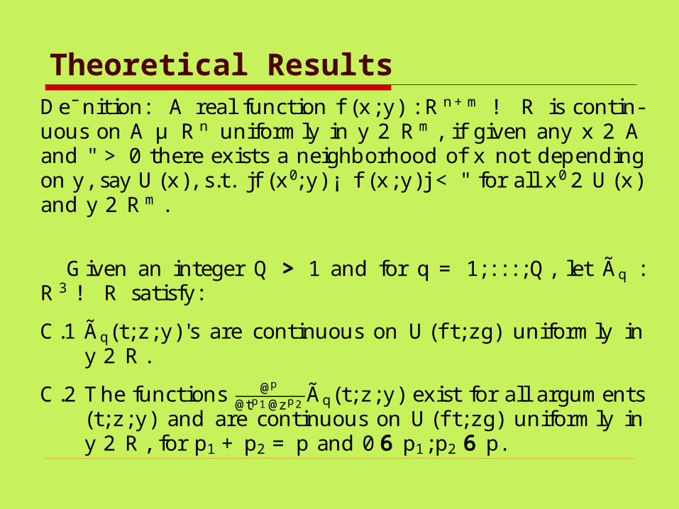
Theoretical ResultsDe nition: A real function f (x; y) : R n +m ! R is contin-uous on A µ R n uniformly in y 2 R m , if given any x 2 Aand " > 0 there exists a neighborhood of x not dependingon y, say U (x), s.t. jf (x0; y) ¡ f (x; y)j < " for all x0 2 U (x)and y 2 R m .

Given an integer Q >>> 1 and for q = 1; : : : ; Q, let Ãq :R 3 ! R satisfy:

C.1 Ãq(t; z; y)'s are continuous on U (f t; zg) uniformly iny 2 R .

C.2 T he functions @p

@tp1 @zp2Ãq(t; z; y) exist for all arguments

(t; z; y) and are continuous on U (f t; zg) uniformly iny 2 R , for p1 + p2 = p and 0 666 p1; p2 666 p.

Notations: 2D Smoothers

T he kernel-weighted averages for two-dimensional smoothersare de ned as:

ª qn =1

nE N hº 1+1¹ ;t hº 2+1

¹ ;z

nXXX

i =1

N iXXX

j =1

Ãq(Ti j ; Z i ; Y i j )K 2(t ¡ Ti j

h¹ ;t;

z ¡ Z i

h¹ ;z):

Let

®q(t; z) =@jº j

@tº 1 @zº 2

ZZZÃq(t; z; y)f 3(t; z; y)dy; and

¾qr (t; z) =ZZZ

Ãq(t; z; y)Ãr (t; z; y)f 3(t; z; y)dykK 2k2;

where f 3(t; z; y) is the joint density of (T; Z; Y ),kK 2k2 =

RRRK 2

2 and 1 666 q; r 666 Q.

Theoretical Results: 2D Smoothers

T heorem 1. Let H : R Q ! R be a function with continuous¯rst order derivatives, D H (v) = ( @

@x1H (v); : : : ; @

@xQH (v))T ,

and ¹N = 1n

PPP ni =1 N i . Under suitable assumptions, and as-

suming h¹ ;z

h¹ ;t! ½¹ and nE (N )h2j· j+2

¹ ;t ! ¿ 2¹ for some 0 <

½¹ ; ¿¹ < 1 , we can obtainq

n ¹N h2º 1+1¹ ;t h2º 2+1

¹ ;z [H (ª 1n ; : : : ; ª Q n ) ¡ H (®1; : : : ; ®Q )]

D¡! N (¯ H ; [D H (®1; : : : ; ®Q )]T § [D H (®1; : : : ; ®Q )]);

Theoretical Results: 2D Smoothers (cont’d)

where

§ =(¾qr )16 q;r 6 l

¯ H =XXX

k1+k2=j· j

(¡ 1)j· j

k1!k2![ZZZ

sk11 sk2

2 K 2(s1; s2)ds1ds2]

£ fQXXX

q=1

@H

@®q[(®1; : : : ; ®Q )T ]

@k1+k2¡ º1¡ º2

@tk1¡ ®q @zk2¡ º2®q(t; z)g¿¹

q½2k2+1

¹ :

Mean Function: Nadaraya-Watson Est.Corollary 1. Under suitable assumptions, and assuming h¹ ;z

h¹ ;t!

½¹ and nE (N )h6¹ ;t ! ¿ 2

¹ for some 0 < ½¹ ; ¿¹ < 1 :q

n ¹N h¹ ;th¹ ;z[¹ N W (t; z) ¡ ¹ (t; z)]fD¡! N (¯ N W ; § N W );

where

¯ N W =XXX

k1+k2=2

1

k1!k2![ZZZ

sk11 sk2

2 K 2(s1; s2)ds1ds2]¿¹

q½2k2+1

¹

£ f1

f 2(t; z)

@2

@tk1 @zk2®1(t; z) ¡

¹ (t; z)

f 2(t; z)

@2

@tk1 @zk2f 2(t; z)g

§ N W =Var(Y jt; z)

f 2(t; z)kK 2k2; ®1(t; z) = ¹ (t; z)f 2(t; z);

and f 2(t; z) is the joint density of (T; Z ).

Mean Function: Local Linear Est.

Corollary. Under suitable assumptions, and assuming h¹ ;z

h¹ ;t!

½¹ , and nE (N )h6¹ ;t ! ¿ 2

¹ for some 0 < ½¹ ; ¿¹ < 1 :

qn ¹N h¹ ;th¹ ;z[¹ L (t; z) ¡ ¹ (t; z)] D¡! N (¯ L ; § L );

where

¯ L =XXX

k1+k2=2

1

k1!k2![ZZZ

sk11 sk2

2 K 2(s1; s2)ds1ds2]@2

@tk1 @zk2¹ (t; z)¿¹

q½2k2+1

¹

§ L =Var(Y jt; z)

f 2(t; z)kK 2k2;

and f 2(t; z) is the joint density of (T; Z ).

Rate of Convergence

If E(N) < , the rate of convergence for the 2D mean and covariance function is .

- This is the optimal rate of convergence for 2D smoothers with independent data.

If E(N) → , the rate of convergence can be as close to as possible but not equal to .

If , the convergence rate is .

1/3n

2/5n2/5n

iN n

Notations: 3D Smoothers

T he technique of kernel-weighted averages can be ex-tended to three-dimensional smoothers to obtain their asymp-totic normalities. Given an integer Q >>> 1, let #q : R 5 ! Rfor q = 1; : : : ; Q satisfying:

D.1 #q(t; s; z; y1; y2)'s are continuous on U (f t; s; zg) uni-formly in (y1; y2) 2 R 2.

D.2 T he functions @p

@tp1 @sp2 @zp3#q(t; s; z; y1; y2) exist for all

arguments (t; s; z; y1; y2) and are continuous on U (f t; s; zg)uniformly in (y1; y2) 2 R 2, for p1 + p2 + p3 = p and0 666 p1; p2; p3 666 p.

Notations: 3D Smoothers (cont’d)

T he general weighted averages of three-dimensionalsmoothing methods are de ned as:

£ qn (t; s; z) =1

nE (N (N ¡ 1))hº 1+º 2+2G ;t hº 3+1

G ;z

£nXXX

i =1

XXX

16 j 6=k6 N i

#q(Ti j ; Ti k; Z i ; Y i j ; Y i k)K 3(t ¡ Ti j

hG ;t;

s ¡ Ti k

hG ;t;

z ¡ Z i

hG ;z):

Notations: 3D Smoothers (cont’d)

Let

»q(t; s; z) =@jº j

@tº 1 @sº 2 @zº 3

ZZZ#q(t; s; z; y1; y2)f 5(t; s; z; y1; y2)dy1dy2

! qr =ZZZ

#q(t; s; z; y1; y2)#r (t; s; z; y1; y2)f 5(t; s; z; y1; y2)dy1dy2kK 3k2;

where f 5(t; s; z; y1; y2) is the joint density of (T1; T2; Z; Y1; Y2),kK 3k2 =

RRRK 2

3, and 1 666 q; r 666 l.

Theoretical Results: 3D Smoothers

T heorem. Let H : R Q ! R be a function with continuous¯rst order derivatives, D H (v) = ( @

@x1H (v); : : : ; @

@xQH (v))T ,

and ¹N = 1n

PPP ni =1 N i . Under suitable assumptions,

hG ;z

hG ;t! ½G and nE (N (N ¡ 1))h2j· j+3

G ;t ! ¿ 2G

for some 0 < ½G ; ¿G < 1 :

qn ¹N ( ¹N ¡ 1)h2º 1+2º 2+2

G ;t h2º 3+1G ;z f H (£ 1n ; : : : ; £ Qn ) ¡ H (»1; : : : ; »Q )g

D¡! N (°H ; [D H (»1; : : : ; »Q )]T ­ [D H (»1; : : : ; »Q )]);

Theoretical Results: 3D Smoothers (cont’d )

where ­ = (! qr )16 q;r 6 Q and

°H =QXXX

q=1

XXX

· 1+· 2+· 3=j· j

f(¡ 1)j· j

j· j!

ZZZu· 1

1 u· 22 u· 3

3 K 3(u1; u2; u3)du1du2du3g

£dj· j

dt· 1 ds· 2 dz· 3

Z#q(t;s;z;y1;y2)f5(t;s;z;y1;y2)dy1dy2

£@H

@»q(»1; : : : ; »Q )T ¿G

q½2· 3+1

G :

Covariance in fFPCA: Nadaraya Watson Est.

Corollary. Under suitable assumptions, and assuminghG ;z

hG ;t! ½G and

nE (N (N ¡ 1))h7G ;t ! ¿ 2

G for some 0 < ½G ; ¿G < 1 :q

n ¹N ( ¹N ¡ 1)h2G ;thG ;z f ¡ N W (t; s; z)¡ ¡ (t; s; z)g D¡! N (°N W ; ­ N W );

Covariance in fFPCA: Nadaraya-Watson cont’d

where

°N W =1

2f ¾2

1¿1d2

dt2¡ (t; s; z) + ¾2

2¿1d2

ds2¡ (t; s; z) + ¾2

3¿2d2

dz2¡ (t; s; z)g

+f ¾21¿1(

d

dt¡ (t; s; z))(

d

dtg3(t; s; z)) + ¾2

2¿1(d

ds¡ (t; s; z))(

d

dsg3(t; s; z))

+¾23¿2(

d

dz¡ (t; s; z))(

d

dzg3(t; s; z))g=g3(t; s; z);

­ N W =À3(t; s; z)kK 3k2

g3(t; s; z);

and g3(t; s; z) is the joint density of (T1; T2; Z ).

Covariance in fFPCA: Local Linear Smoothers

Corollary. Under suitable assumptions, assuming hG ;z

hG ;t!

½G , and nE (N (N ¡ 1))h7G ;t ! ¿ 2

G for some 0 < ½G ; ¿G < 1 :

qn ¹N ( ¹N ¡ 1)h2

G ;thG ;z f ¡ L (t; s; z) ¡ ¡ (t; s; z)g D¡! N (°L ; ­ L );

where

°L =1

2f ¾2

1¿1d2

dt2¡ (t; s; z) + ¾2

2¿1d2

ds2¡ (t; s; z) + ¾2

3¿2d2

dz2¡ (t; s; z)g

­ L =À3(t; s; z)kK 3k2

g3(t; s; z);

and g3(t; s; z) is the joint density of (T1; T2; Z ).

Covariance in mFPCA: Local Linear SmoothersCorollary. Under suitable assumptions, hG ¤ ! 0,nE (N 2)h2

G ¤ ! 1 , hG ¤ E (N 3) ! 0, nE (N (N ¡ 1))h6G ¤ ! ¿ 2

for some 0 666 ¿ < 1 , we can obtainq

n ¹N ( ¹N ¡ 1)h2G ¤ f ¡ ¤(t; s) ¡ ¡ ¤(t; s)g D¡! N (° ¤; ­ ¤);

where

° ¤ =¿

2

ZZZu2K 1(u)duf

d2

dt2¡ ¤(t; s) +

d2

ds2¡ ¤(t; s)g;

­ ¤ =À2(t; s)kK 1k4

g2(t; s);

À2(t; s) =Var((Y1 ¡ ¹ (T1; Z ))(Y2 ¡ ¹ (T2; Z ))jT1 = t; T2 = s);

and g2(t; s) is the joint density of (T1; T2).

Rates of Convergence

If E(N) < , the rate of convergence for the 3D covariance is , which is the optimal rate of convergence for independent data.

If E(N) → , the rate of convergence can be as close to as possible, but not equal to it.

If , the convergent rate should be .

2/7n

iN n

2/5n

Theorem 3: Eigen-values/functions in mFPCA

T heorem. Let n´ ¡ (1=3) 666 h¹ = o(1) for some ´ > 0, andassume that for an integer j 0 > 1 there are no ties amongthe (j 0 + 1) largest eigenvalues of ¡ ¤(t; s); that

(i) n´ 1¡ (1=3) 666 hG ¤ for some ´1 > 0, h¹ = o(hG ¤ ),max(n¡ 1=3h(2=3)

G ¤ ; n¡ 1h(¡ 8=3)G ¤ ) = o(h¹ ), and hG ¤ = o(1)

(ii) n´ ¡ (3=8) 666 hG ¤ , and hG ¤ + h¹ = o(n ¡ 1=4):

A lso, let ¤ = (¸ 1; : : : ; ¸ j 0 )T , and ¤ = (^1; : : : ; ^

j 0 )T .

Theorem 3 (cont’d) :

Let N ¤ = 12

PPP ni =1 N i (N i ¡ 1):

Under assumptions (i),

kÁj ¡ Áj k2 =C 1j

N ¤hG ¤+ C 2j h4

G ¤ + opf (nhG ¤ )¡ 1 + h4G ¤ g;

and under assumptions (ii):

pn(¤ ¡ ¤ ) is asymptotically a multivariate normal dis-

tribution with mean 0 and covariance matrix § .

Optimal Rates of Convergence

The first k eigenfunctions can be estimates at the same optimal rate as a 1-dim nonprametric regression function.

The largest k eigenvalues can be estimated at the rate. n

Bandwidth Selection

² M ean Function ¹ (t; z) and covariance ¡ ¤(s; t) :

Leave one subject out cross-validation

² Covariance Function ¡ (s; t; z): k-fold cross-validation

Suppose that the subjects are randomly assigned to ksets (S1; S2; : : : ; Sk).

h = argminh

kXXX

l=1

XXX

i 2 S l

XXX

16 j 6=m 6 N i

f C i j m ¡ ¡ (¡ Sl )(Ti j ; Ti m ; zi )g2;

where ¡ (¡ Sl )(Ti j ; Ti m ; zi ) is the estimated covariance func-tion at (Ti j ; Ti m ; zi ) when the subjects in S l are not usedto estimate ¡ (t; s; z).

Number of Eigenfunctions

We used three methods:

AIC

BIC

FVE: minimum number of eigen-components needed to explained at least a specified total fraction of the variation.

Predicted Trajectory for X(t)

Suppose that the ¯rst K eigenfunctions are used to pre-dict the trajectories; given t 2 T and z 2 Z , the predictedtrajectory of X i (t; z) based on the ¯rst K eigenfunctionswill be

X Ki (t; z) = ¹ L (t; z) +

KXXX

k=1

A i k(z)Ák(t; z) (fFP CA )

X Ki (t; z) = ¹ L (t; z) +

KXXX

k=1

A ¤i kÁ¤

k(t) (mFP CA )

Simulation Study

² Let covariate Z » U (0; 1)

² ¹ (t; z) = t + z sin (t) + (1 ¡ z) cos(t)

² Á1(t; z) = ¡ cos(¼(t + z=2))p

2 andÁ2(t; z) = sin (¼(t + z=2))

p2

² ¸ 1(z) = z=9, ¸ 2(z) = z=36 and ¸ k(z) = 0 for k >>> 3.

² A i k » N (0; ¸ k(z))

² measurement errors » N (0; 0:052)

T he simulation consists of 100 runs.T he number of subect is 100 in each run.

True and Estimated Mean Surface

Simulation: Estimated Eigenfunctions (mFPCA)

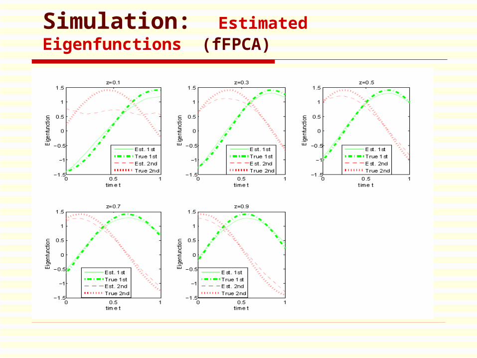
Simulation: Estimated Eigenfunctions (fFPCA)

Simulation Studycovariate z 0.1 0.3 0.5 0.7 0.9I SE of ¡ L 0.00015 0.00025 0.00071 0.0014 0.0030

I SE of Á1(t; z) 0.0294 0.0076 0.0071 0.0074 0.0112I SE of Á2(t; z) 0.2720 0.0305 0.0242 0.0179 0.0300

^1(z) 0.0047 -0.0041 -0.0113 -0.0202 -0.0242(0.0073) (0.0106) (0.0181) (0.0205) (0.0333)

^2(z) 0.0034 0.0001 0.0005 -0.0002 -0.0037(0.0045) (0.0039) (0.0057) (0.0077) (0.0094)

Simulation results of fFP CA . T he three rows correspond-ing to ISE are based on the average integrated squared er-rors of the 100 simulations, and the rows corresponding to^

i are the biases and standard deviation (in bracket).

Simulation Study

M I SE M SF EF V E A IC BI C F V E A I C BI C

uF P CA 0.0325 0.0198 0.0197 0.0067 0.0065 0.0065mF P CA 0.0103 0.0063 0.0063 0.0050 0.0017 0.0017

fF P CA 0.0085 0.0077 0.0077 0.0022 0.0015 0.0015

M I SE =1

n

nXXX

i = 1

ZZZ 1

0(X i (t; zi ) ¡ X K

i (t; zi ))2dt

M SF E =1

n

nXXX

i = 1

1

N i

N iXXX

j = 1

(Y i j ¡ Y i j )2:

.

Conclusions

² T hrough simulations and data analysis, we have shownthat current approaches for functional principal com-ponent analysis are no longer suitable for functionaldata when covariate information is available.

² Numerical evidence supports the simpler mean-adjustedapproach especially when the purpose is to predict thetrajectories Y (t).

² T he catch is the high-dimensional smoothing involvedwith a vector Z . Some dimension reduction on Z willbe needed for practical implementation and this willbe a future research project.

End of Single Covariate

* Multidimensional Covariates

T T T1 2 k

T

,

k<p

single i

Assume that and only the mea

(t, z)= (t, z)

(t, z)= (t, z, z, ...,

n function depends on Z.

nde or

, )z

multiple indices

x

pZ

Dimension Reduction Models

There are many ways to estimate the indices for independent data, i.e. when there is no t.

Few has been extended to longitudinal or functional data, but none for the multi-index model

We choose an approach “MAVE” by Xia et al. (2002) to extend to longitudinal data.

T T T1 2 k= ( z, z, ..., z .)+Y

T T T1 2 k( ) = ( , z, z, ..., z)+ ( ).t t tY

- convergence of

T heorem. Let ^ be the estimator of ¯ 0 in the algorithm.Under some regularity conditions, we have

pn( ^¡ ¯ 0) ¡ ! D N (0; § );

where

§ =[E (G(T; Z ))]+ § ¤[E (G(T; Z ))]+ ;

G(t; z) =µ

d¹ (t; ¯ T0 z)

d(¯ T0 z)

¶2 ¡zzT ¡ m(t; z)m(t; z)T

¢;

G0(t; z) =µ

d¹ (t; ¯ T0 z)

d(¯ T0 z)

¶(z ¡ m(t; z));

m(t; z) =E (Z jT = t; ¯ T0 Z = ¯ T

0 z);

and A + is the M oore-Penrose inverse of matrix A .

n

- convergence of

§ ¤ =E N ¡ 1

E NE (f G0(T; Z )²gf G0(T; Z )²)gT )

+1

E NE (f G0(T; Z )²gf G0(T; Z )²gT )

n

AIDS CD4: Estimated Mean

AIDS: Estimated Covariance + measurement error

End of Multidimensional Covariates

­­3. What’s Next After FPCA?­

FPCA can be the end product - to explore the covariate effects, to recover the trajectories of each subject, and to explore the modes of variation etc.

FPCA can help to find more parsimonious model.

AIDS CD4: Estimated Mean

AIDS CD4 Data

This suggests the possibility of a more parsimonious model with multiplicative covariate effects.

could be parametric, e.g. a polynomial.

Common marginal models for longitudinal data take the additive form, and employ parametric models for both the mean and covariance function.

- Both parametric forms are difficult to detect for sparse and noisy longitudinal data.

( ) ( ) ( ) ).(TY t t z e t ( )t

AIDS CD4: Estimated Covariance

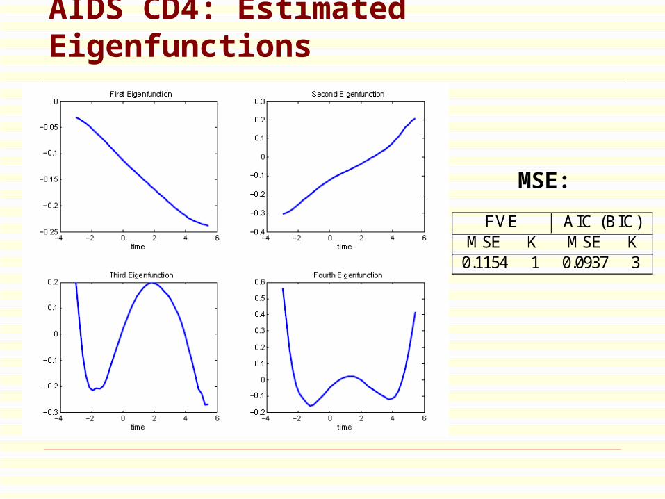
AIDS CD4: Estimated Eigenfunctions

FVE AIC (BIC)MSE K MSE K

0.1154 1 0.0937 3

MSE:

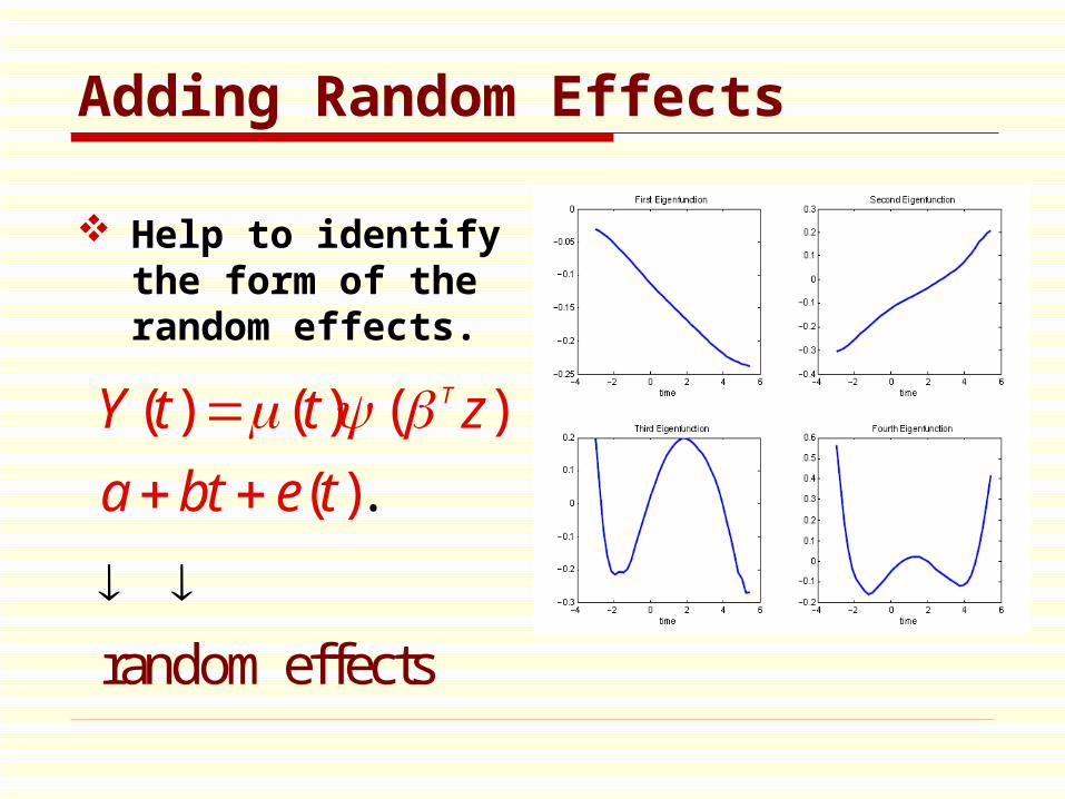
Adding Random Effects

Help to identify the form of the random effects.

( ) ( ) ( )

( .

random

)

e cts

ffe

TY t t z

a bt e t

Semiparametric Product Model

If we assume that the first eigenfunction is proportional to the population mean function , and discards the remaining eigenfunctions, we arrive at the following multiplicative random effect model:

Random effects

( ) ( , ) ( , ) ( ) ( , ) ( .)Y t t z A t z e t

b t z e t

( , )t Z

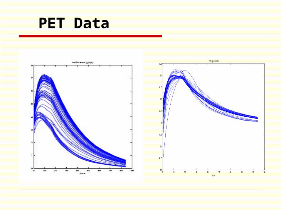
­­PET Data

0 10 20 30 40 50 60 70 80 90-0.2

-0.15

-0.1

-0.05

0

0.05

0.1

0.15

0.2

0.25

time

First Eigenfunction

4. Dynamic Positron Emission Tomography (PET) Time Course Data

Joint work with

Ciren Jiang , UC Davis

&

John Aston

Academia Sinica & Univ. of Warwick

John Aston, Academia Sinica & Warwick U.

Dynamic PET Time-Course Data PET is a nuclear medicine imaging technique

which produces a three-dimensional image or picture of functional processes in the body.

A PET scan measures important body functions, such as blood flow, oxygen use, and sugar (glucose) metabolism, to help doctors evaluate how well organs and tissues are functioning.

Measured 11C-Diprenorphine Data

The scan is an experiment on epilepsy. The chemical compound Diprenorphine measures the concentration of opioid (pain) receptors in the brain.

The idea of the overall experiment was to see if there was a difference in the concentration of receptors in Epileptics against normal subjects.

However, the changes that were hypothesized were very small so it was important that the experiment could get as accurate measurements as possible.

Measured 11C-Diprenorphine Data

A dynamic scan from a measured 11C-diprenorphine study of a normal subject were analyzed.

Four Dimensional Data: three spatial + one temporal 128 × 128 × 95 × 32

Voxel sizes were 2.096 mm × 2.096 mm × 2.43 mm.

Scans were rebinned into 32 time frames of increasing duration.

t = 27.5, 60, 70, 80, 100, 130, ..., 1075, 1195, 1315, ..., 4435, 5035 seconds

Example of Analysis for five voxels

Motivation

Due to experimental constraints, the time course measurements are often fairly noisy.

The Spectral Analysis method (Cunningham and Jones, 1993) is well known to be sensitive to noise with the bias being highly dependent on the level of noise present.

By borrowing information across space through the use of a non-parametric covariate adjustment, it is possible to reconstruct the PET time course data and thus reduce noise.

Many of the processes presented in the PET time course data have chemical rates associated with them. These rates are dependent on a large number of biological factors, too numerous and complex to be exhaustively represented or identified in the discretely and noisily measured data.

However, if an alternative viewpoint that the rates are random variables is taken, then a small additive random change in one rate will lead to a multiplicative change in the time course.

Motivation

Multiplicative Nonparametric Random Effects Model

Since Á1(t; z) / ¹ (t; z), from the random curve view-point the concentration curve of the voxel i with covariatezi can be represented as

X i (t; zi ) = ¹ (t; zi ) +1XXX

k=1

A i kÁk(t; zi )

= B i ¹ (t; zi ) +1XXX

k=2

A i kÁk(t; zi );

where B i = 1 + ®A i 1 and Á1(t; z) = ®¹ (t; z).

Estimation Procedures

² Determine in-brain voxels

² A pply 2D smoother to the setf (Y i j ; tj ; zi )ji = 1; : : : ; n; 1 666 j 666 pg to estimate ¹ (t; z)

² A pply least squares method to estimate B i

² A pply 3D smoother to the setf (G i j k; tj ; tk; zi )ji = 1; : : : ; n; 1 666 j 6= k 666 pg to estimate¡ (t; s; z), whereG i j k = (Y i j ¡ B i ¹ (tj ; zi ))(Y i k ¡ B i ¹ (tk; zi ))

Estimation Procedures

² Estimate ¸ k(z) and Ák(t; z), and apply FV E to choosethe number of eigenfunctions

² A pply Integration M ethod to estimate the principalcomponent scores A i k(zi )

² R econstruct the random curve for each voxel:X K

i (t) = B i ¹ (t; zi ) +PPP K

k=2 A i k(zi )Ák(t; zi )

² A pply parametric method to the reconstructed curves.

Variable Bandwidth b(t)

A global bandwidth is appropriate along the covariate coordinate, but not desirable in the time coordinate.

denser measurement schedule at the beginning and sharp peak near the left boundary

Smaller bandwidths are preferred near the peak, while larger bandwidths are used near the right boundary.

Choose Variable Bandwidth b(t)

choose 13 time locations.

[t-b(t), t+b(t)] includes at least four observations

boundary correction to ensure a positive bandwidth

To ensure a smooth outcome, fit a polynomial of order 4 to the pairs (tj, b(tj)).

The resulting b(t) is further multiplied by a constant α, determined by a cross-validation step.

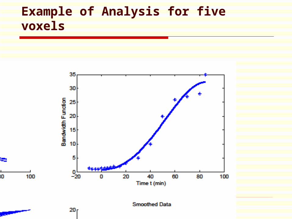
Example of Analysis for five voxels

Spectral Analysis (Cunningham and Jones, 1993)

Spectral A nalysis does not assume a known compart-mental structure, but rather performs a model selectionthrough a non-negativity constraint on the parameters. Inparticular, the concentration curve X (t) is parameterizedby

X (t) = I (t)O KXXX

j =1

®j exp ¡ ¯ j t;

where I (t) is a known input function and ®j and ¯ j are thenon-negative parameters to be estimated.

T he parameter of interest VT is the integral of the im-pulse response function

VT =ZZZ 1

0

KXXX

j =1

®j exp ¡ ¯ j tdt =KXXX

j =1

®j

¯ j:

Conclusions

This is consistent with the knowledge that Spectral Analysis has high positive bias at voxel noise levels of around 5%. By reconstructing the data through fFPCA, the noise level is reduced, and thus the level of bias is also reduced. (Overall mean squared residuals reduce 71.82%)

The covariate adjusted FPCA can be applied in practice to measured PET data using spatially pooled information.

Thank You

The End

Sedona, Arizona, 2006 IMS WNAR

Covariate adjusted FPCA: Longitudinal Data

We propose two ways:

fFPCA & mFPCA.

Both consist of two parts:

a systematic part for the mean function and a stochastic part for the covariance function.

Difference - handling of the covariance structure