course 02283, f2011, lecture notes on randomized search heuristics

Course 02283, F2011, Lecture Notes onRandomized Search Heuristics

Carsten Witt

Version 0.41 (April 2, 2011)

1 Introduction

This part of the course deals with randomized search for optimization problems,more precisely bio-inspired randomized search heuristics such as evolutionary algo-rithms, simulated annealing etc. Such general heuristics are applied “off-the-shelf”when it is not possible to apply an algorithm tailored to the problem at hand. Rea-sons for this are lack of resources such as time, money, knowledge etc.

Practitioners report surprising success of randomized search heuristics on op-timization problems, but a theoretical foundation has been built up only recently.The aim of this part of the course is to contribute to the understanding of random-ized search heuristics from an algorithmic viewpoint using methods from classicaltheoretical computer science.

2 Preliminaries

We consider two very simple randomized search heuristics for the search space{0, 1}n, where the aim is to find a bit string that optimizes a so-called fitnessfunction f : {0, 1}n → R. The search heuristics are called RLS (Algorithm 1)and (1+1) EA (Algorithm 2). They only differ in Step 3, the so-called mutation.Common of both is that they start with a uniformly at random selected searchpoint, proceed in rounds and replace search points if and only if the new searchpoint created by mutation is at least as good as the previous one. The mutationoperator of RLS flips exactly one bit, while the number of bits flipped by the(1+1) EA is random. It can be between 0 and n and is n⋅(1/n) = 1 in expectation.

The algorithms as presented here do not use a stopping criterion, which wouldbe needed in practical implementations. For our theoretical purposes, we can ana-lyze the search heuristics as infinite stochastic processes. We are mainly interested

1

in the first point of time TA,f such that algorithm A (so far only RLS or (1+1) EA)has created a search point that is optimal for f . Each time step contains one eval-uation of f , hence TA,f basically counts the number of f -evaluations until reachingthe optimum, which is the common cost measure (sometimes called black-boxmeasure) in the analysis of randomized search heuristics. The reason is that anevaluation of a complicated fitness function is typically the most expensive part inexperiments, while the other steps of the algorithm are cheap and computationallyneglegible. Since we do not always know how the concrete fitness function works(it is a so-called black box), we always set up one time unit for an evaluation.

We call TA,f the optimization time or simply runtime of A on f and note thatthis is a random variable. As usual in the analysis of randomized algorithms,the expected value E(TA,f ) is of particular interest and is referred to as expectedoptimization time or, synonymously, expected runtime. Finally, optimization maymean that we minimize or maximize a function. The algorithms are defined formaximization problems, which is without loss of generality since maximizing f isequivalent to minimizing −f .

Algorithm 1 Randomized Local Search (RLS)

1. t := 0. Choose x = (x1, . . . , xn) ∈ {0, 1}n uniformly at random.

2. y := x

3. Choose one bit in y uniformly at random and flip it (mutation).

4. If f(y) ≥ f(x) Then x := y (selection).

5. t := t+ 1. Continue at line 2.

Algorithm 2 (1+1) Evolutionary Algorithm ((1+1) EA)


2. y := x

3. Independently for each bit in y: flip it with probability 1n

(mutation).

4. If f(y) ≥ f(x) Then x := y (selection).


2

3 (1+1) EA and RLS on Example Problems

Randomized search heuristics were defined without a theoretical analysis in mind.Instead, the aim was to follow biological ideals such as evolution (“‘survival of thefittest”), which makes them harder to analyze than classical algorithms, where thedesigner had a proof of correctness, runtime etc. already in mind when publishingthe algorithm. In order to develop first results, initial research focused on so-called example problems of a simple structure. Even on these problems, it isnot obvious how randomized search methods behave. Methods from probabilitytheory and algorithmics had to be adjusted to randomized search heuristics andthe stochastic processes behind them. In the course of this and the subsequentsections, we develop proof techniques along with the results presented.

3.1 Upper Bounds

We start with a very general result, whose proof presents the first general tech-nique.

Theorem 1. Let f : {0, 1}n → R be arbitrary. The expected optimization time ofthe (1+1) EA on f is at most nn.

Proof. Let x∗ be a search point that has maximal f -value. For any current searchpoint x, the probability of creating x∗ by mutation of x is(

1

n

)H(x,x∗)(1− 1

n

)n−H(x,x∗)

,

where H(x, x∗) is the Hamming distance (see Appendix) of x∗ and x. The reasonis that exactly those bits where x and x∗ differ need to be flipped. Obviously, theprobability becomes smallest (assuming n ≥ 2) if H(x, x∗) = n and is (1/n)n then.In each step, we have this minimum probability, hence the waiting time argument(see Appendix) tells us that we have to wait for an expected number of at most1/(1/n)n = nn steps until x∗ is created.

For RLS, we do not have any general upper bound on the expected optimizationtime except for the trivial bound∞. The reason is that RLS might fail to optimizefunctions since it would have to change 2 or more bits for an improvement, whichis not possible with RLS’s mutation operator; in such a case, one says that RLS isstuck in a local optimum. Theorem 1 tells us that the (1+1) EA cannot get stuckand will eventually optimize every function, but the bound is exponential. Later(Theorem 7), we will see that the bound is tight, i. e., that on certain functionsnΩ(n) steps are needed.

3

On well-structured problems, we expect randomized search heuristics to bemuch faster than nn. One of the most famous example problems is

OneMax(x1, . . . , xn) = x1 + ⋅ ⋅ ⋅+ xn,

which just returns the number of one-bits in the current search point. Of course, ifthe randomized search heuristic knew that it is optimizing OneMax, it would betrivial to state the optimum, namely the string of all-ones. However, randomizedsearch heuristics do not know the fitness function since they are general black-boxalgorithms that only evaluate the function by querying search points. Nevertheless,our two search heuristics optimize OneMax fairly efficiently, as will be shown inthe following theorem.

Theorem 2. The expected optimization time of RLS and the (1+1) EA on One-Max is O(n log n).

Proof. We start with a general observation. The fitness function OneMax de-pends only on the number of one-bits, and both search heuristics do not careabout the positions of the bits in the current search point; namely, RLS selectsthe bit to flip randomly and (1+1) EA considers each bit independently withouttaking the position of the bits into account. It is therefore safe to consider only thenumber of one-bits in the current search point, no matter where these are. Moreformally, we compress the state space of the search heuristic to {0, . . . , n}, wherestate i means that the current search point has i one-bits.

Let us first consider RLS. If the current search points has i one-bits, there aren−i out of n good outcomes of the mutation, namely those that flip a zero-bit. Allother mutations lead to a search point with inferior fitness, which will be rejected.Hence, the probability of improving the number of one-bits by 1 is exactly (n−i)/nin this situation. The expected time for this to happen (waiting time argument)is n/(n − i). Each value of i has to be considered at most once, since the fitnessof the current search point will not decrease. Pessimistically assuming that everyvalue occurs once (i. e., assuming we start with no one-bit) gives us the expectedoptimization time

n−1∑i=0

n

n− i= n

n∑i=1

1

i≤ n(lnn+ 1) = O(n log n),

where we have used∑n

i=11i≤ (lnn) + 1 (a bound for the so-called Harmonic

number, see Appendix).With the (1+1) EA, the argumentation is similar. However, this search heuris-

tic might flip several bits in a step, and it is difficult to argue about such steps.

4

Instead, we concentrate on the steps that flip only a single bit, more precisely azero-bit in the current search point. The probability of such a step is

(n− i) 1

n

(1− 1

n

)n−1

≥ n− ien

,

where we used that there are n − i zero bits, each of which flips with probability1/n, while n − 1 bits do not flip with probability 1 − 1/n each; finally, we haveused the estimate (1 − 1/n)n−1 ≥ 1/e (see Appendix). Continuing as in the caseof RLS, the expected optimization time of (1+1) EA is at most

n−1∑i=0

en

n− i= en

n∑i=1

1

i= O(n log n),

which completes the proof.

Remark: The argumentation for the case of RLS is well known in the theoryof randomized algorithms as the “Coupon Collector’s Problem” (Motwani andRaghavan, 1995). The scenario is that there are n initially empty bins, and astochastic process throws at each time step one ball into a uniformly chosen bin.It takes Θ(n log n) expected steps until each bin contains at least one ball, whichresult we have proved above noting that ”we throw one-bits”. This analogy showshow classical algorithms theory helps to analyze the stochastic processes behindrandomized search heuristics. However, we also see that we cannot apply thecoupon collector’s problem in its pure form to the (1+1) EA. Here we had toadapt the method towards our stochastic process.

As said above, one aim behind the analysis of simple problems like OneMax isto develop an understanding of the search heuristics and general techniques for theanalysis. It turns out that the proof method from Theorem 2 can be generalizedas follows. We partition the search space into levels of “roughly” the same fitnessand consider the progress of the search heuristics through the levels.

Definition 1 (Fitness-based partition). Let f : {0, 1}n → R be given. ThenL0, L1, . . . , Lk ⊆ {0, 1}n is called a fitness-based partition with respect to f iff

1. ∀i ∈ {0, 1, . . . , k} : Li ∕= ∅2. ∀i ∕= j ∈ {0, 1, . . . , k} : Li ∩ Lj = ∅

3.k∪i=0

Li = {0, 1}n

4. ∀i < j ∈ {0, 1, . . . , k} : ∀x ∈ Li : ∀y ∈ Lj : f(x) < f(y)

5. Lk = {x ∈ {0, 1}n ∣ f(x) = max{f(x′) ∣ x′ ∈ {0, 1}n}}

5

The first three conditions from Definition 1 just specify that L0, . . . , Lk parti-tions the search space into non-empty, non-overlapping sets. The fourth conditiontells us that every search point in a set with a certain index has higher fitness(i. e., f -value) than all search points in all sets with smaller index. Finally, theset with largest index contains only optimal search points, i. e., those with max-imal f -value. In the proof of Theorem 2, we implicitly considered the partitionLi := {(x1, . . . , xn) ∣ x1 + ⋅ ⋅ ⋅+ xn = i} for 0 ≤ i ≤ n.

A fitness-based partition will be used in the following way to derive upperbounds on the expected optimization time of RLS and the (1+1) EA. Suppose wehave for each level a lower bound on the probability of leaving the level. Since oursearch heuristics do not accept search points of lower fitness, each level can be leftat most once; in fact certain levels might be left out. Summing up the waitingtimes on all levels, we obtain the following general upper bound.

Theorem 3 (Fitness-level method). Consider the (1+1) EA or RLS on a functionf : {0, 1}n → ℝ and suppose an f -based partition L0, L1, . . . , Lk is given. Let forall i ∈ {0, 1, . . . , k − 1}

si := minx∈Li

Prob(mutate x into some y ∈ Li+1 ∪ ⋅ ⋅ ⋅ ∪ Lk).

Then the expected optimization time on f is at most∑k−1

i=01si

.

Proof. As mentioned above, each fitness level is left as most once. As long as thesearch heuristic is in level i, there is a lower bound si on the probability of leavingthe level, and the expected time for this to happen is at most 1/si by the waitingtime argument. Summing up the 1/si for all levels yields the theorem.

The proof of Theorem 2 used si = (n − i)/n and si = (n − i)/(en) for RLSand (1+1) EA, respectively. As an additional application, we consider anotherwell-known example function, namely

BinVal(x1, . . . , xn) :=n∑i=1

2n−i ⋅ xi,

which returns the integer value of the bit string with x1 being the most significantbit.

Theorem 4. The expected optimization time of the (1+1) EA and RLS on Bin-Val is O(n2).

Proof. We use

Li := {x ∣ 2n−1+2n−2+⋅ ⋅ ⋅+2n−i ≤ BinVal(x) < 2n−1+2n−2+⋅ ⋅ ⋅+2n−i+2n−i−1},

6

where 0 ≤ i ≤ n, as fitness-based partition. By studying the intervals whichmake up the sets Li, it immediately follows that L0, . . . , Ln partitions the wholesearch space (first three properties from Definition 1) and is fitness-based (last twoproperties). Moreover, since 2k ≤

∑k−1j=0 2j holds for all k ≥ 0, it follows see that

a search point is in level i if and only if the bits with index 1, . . . , i are all 1 whilebit i+ 1 is 0. Note that the remaining n− i−1 bits are arbitrary, hence Li (i < n)contains 2n−i−1 search points.

In order to advance from Li to a level of higher index, it is sufficient to flipbit i+ 1 and leave the other bits unchanged. The corresponding probability is 1/nfor RLS and (1/n)(1 − 1/n)n−1 ≥ 1/(en) for the (1+1) EA. (Recall the proof ofTheorem 2 if these estimations are unfamiliar.) Hence, defining si := 1/(en) is inaccordance with Theorem 3 for both heuristics. Consequently,

∑n−1i=0 1/si = en2 =

O(n2) is an upper bound on the expected optimization time.

3.2 Lower Bounds

Of course, it is interesting to know whether the previously proven upper boundsare tight or whether they can be improved. Therefore, we supply lower bounds onOneMax and another example function in this subsection.

Theorem 5. The expected optimization time of RLS and the (1+1) EA on One-Max is Ω(n log n).

Proof. For both search heuristics, we consider the number X of one-bits in theinitial search point. Since this one is drawn uniformly, each bit is set to 1 withprobability 1/2, and we obtain E(X) = n/2. Moreover, Chernoff bounds (seeAppendix) tell us that Prob(X > (2/3)n) = 2−Ω(n) holds, hence with overwhelmingprobability the initial search point has at least n/3 zero-bits. Let A denote theevent that this happens. In the following, we consider the expected optimizationtime under the condition of A. Using the law of total probability (see Appendix)we obtain E(T ) ≥ E(T ∣ A) Prob(A) ≥ E(T ∣ A)⋅(1−2−Ω(n)) for the unconditionalexpected optimization time E(T ).

With RLS, the number of one-bits increases by at most 1 in every step andthe probability of improving from i to i+ 1 one-bits is exactly (n− i)/n. Arguinganalogously to the proof of Theorem 2 and using the bound

∑ki=1 1/i ≥ ln k (see

Appendix), we obtain

E(TRLS,OneMax ∣ A) ≥n−1∑

i=(2/3)n

n

n− i= n

n/3∑i=1

1

i≥ n ln(n/3) = Ω(n log n),

hence also E(TRLS,OneMax) = Ω(n log n).

7

With the (1+1) EA, the arguments from the preceding paragraph do not work.Instead, we take a more direct approach. The aim is to show (still assumingevent A) that with probability at least c1 for some constant c1 > 0 it happensthat at least one of the at least n/3 zero-bits from the initial search point is neversubject to mutation in a period of c2n lnn steps for some constant c2 > 0. Ifwe manage to prove this statement, then the law of total probability still givesus a bound of c1c2n lnn on the expected optimization time (given A), altogetherΩ(n log n) for the unconditional expected optimization time.

To prove the statement, fix an arbitrary bit i. Obviously, Prob(i flips) = 1n

and the probability that i does not flip equals 1 − 1n

for every single step of the(1+1) EA. Moreover, due to the independence of the mutations over several steps,we obtain for every t > 0 that Prob(i does not flip in t steps) = (1− 1

n)t, and the

probability that i flips at least once in t steps equals 1−(1− 1n)t. Since the mutation

operator of the (1+1) EA treats all bits independenly also while performing themutation steps, we have that n/3 specific bits all flip at least once in t steps withprobability (1− (1− 1

n)t)n/3 and, finally,

Prob

(∃ bit out of n

3specific bits

that never flips in t steps

)= 1−

(1−

(1− 1

n

)t)n/3

.

We are left with finding an appropriate value for t. This can be found havingin mind the estimations (1−1/n)n ≤ 1/e ≤ (1−1/n)n−1 and using some intuition.We verify that t := (n− 1) lnn is a good choice.

Prob(∃ bit out of n3

specific bits that never flips in t steps)

= 1−

(1−

(1− 1

n

)(n−1) lnn)n/3

≥ 1−

(1−

(1

e

)lnn)n/3

= 1−(

1− 1

n

)n/3≥ 1−

(1

e

)1/3

> 0.28,

where we used (1 − 1/n)n−1 ≥ 1/e in the first “≥” and (1 − 1/n)n ≤ 1/e in thesecond “≥”. Since c2 := 0.28 does not depend on n and t = c1n lnn for c1 = 0.5,the desired statement has been shown and the proof is complete.

Taking the previous proof and the upper bounds from Theorem 2 together, weobtain the following asymptotically tight bound.

Corollary 1. The expected optimization time of RLS and the (1+1) EA on One-Max equals Θ(n log n).

8

One might wonder whether there are functions on which the search heuristicsare faster. Reconsidering the proof of Theorem 5, we actually have proven a muchmore general result, showing that the lower bound Ω(n log n) cannot be beatenunless the function is very simple.

Theorem 6. Let f : {0, 1}n → ℝ be a function with a unique optimum. Then theexpected optimization time of RLS and the (1+1) EA on f is Ω(n log n).

Proof. Let x∗ be the unique search point that optimizes f . In the initial searchpoint, every bit is set to the corresponding value in x∗ with probability exactly 1/2,hence the event A that x differs from x∗ in at least n/3 bits occurs with probabilityat least 1 − 2−Ω(n). Consequently, with the (1+1) EA we proceed as in the proofof Theorem 5 by considering “wrongly” intialized bits instead of zero-bits.

With RLS, the proof is an exercise.

Finally, we investigate the general upper bound from Theorem 1. It turns outto be tight by virtue of the following function.

Define

Trap(x1, . . . , xn) :=

{x1 + ⋅ ⋅ ⋅+ xn if x1 + ⋅ ⋅ ⋅+ xn ≥ 1,

n+ 1 otherwise.

Except for the all-zeros string, the Trap function equals OneMax. However, theoptimal search point is the all-zeros string, not the all-ones string. Typically, asearch heuristic will follow the OneMax-like structure in order to arrive at theall-ones string. There it will be trapped in a sense that all bits have to be changedat once in order to reach the optimum.

Theorem 7. The optimization time of the (1+1) EA on Trap is at least nn/2

with probability 1− 2−Ω(n). For RLS, it is infinite with probability 1− 2−Ω(n).

Proof. The idea is to consider a so-called typical run of either heuristic. Let A1

be the event that the initial search point has at least n/3 zero-bits. Let A2 bethe event that the search heuristic optimizes OneMax within at most c2nn log nsteps for some constant c to be chosen later. Let A3 be the event that the searchheuristic does not flip n/3 or more bits in a single step of the first c2nn log n steps.If A∗ := A1∩A2∩A3, i. e., all three events together, occur, the run is called typical.We will show later that Prob(A∗) = 1− 2−Ω(n).

Let us consider a typical run. Hence, after at most c2nn log n steps the all-onesstring is reached, which is the second-best point. To create the optimum, all bitshave to flip at once, which has probability (1/n)n for the (1+1) EA and is impos-sible for RLS. Using the law of total probability to take into account Prob(A∗)(see the proof of Theorem 5 for the first application of this technique), we already

9

obtain the lower bound for RLS. With regard to the (1+1) EA, the probabil-ity of reaching the optimum is (1/n)n in every step t where the all-ones stringis the current search point. Therefore, the probability of reaching the optimum

within T := nn/2 steps is at most∑nn/2

t=1 (1/n)n = n−n/2 by the union bound. Theprobability that this happens or that the run is not typical is altogether at mostn−n/2 + 2−Ω(n) = 2−Ω(n), which proves the theorem for the (1+1) EA assumingProb(A∗) = 1− 2−Ω(n).

We are left with the claim on Prob(A∗). We have already argued in the proofof Theorem 5 that Prob(A1) = 1−2−Ω(n) follows by Chernoff bounds. With regardto A2, recall (Theorem 2 that the expected optimization time of the (1+1) EA onOneMax is at most cn log n for some constant c > 0, hence it is at most c2nn log nwith probability at least 1− 2−n using Markov’s inequality (see Appendix).

With regard to A3, observe that the probability of flipping at least n/3 bits ina single step is at most(

n

n/3

)⋅(

1

n

)n/3≤ nn/3

(n/3)!

(1

n

)n/3=

1

(n/3)!≤(

3e

n

)n/3,

where we used the inequalities(nk

)≤ nk/k! and k! ≥ (k/e)k (see also the Ap-

pendix). Using a union bound similarly as in the preceding paragraph, the prob-ability that at least n/3 bits flip in at least one out of c2nn log n steps is at most(c2nn log n)(3e/n)n/3 = 2−Ω(n), which proves Prob(A3) = 1− 2−Ω(n). We concludethe proof by noting that Prob(A∗) = 1 − Prob(A∗) = 1 − Prob(A1 ∪ A2 ∪ A3) ≥1− (2−Ω(n) + 2−Ω(n) + 2−Ω(n)) = 1− 2−Ω(n), where we applied De Morgan’s law toconclude A1 ∩ A2 ∩ A3 = A1 ∪ A2 ∪ A3 and finally used a union bound.

We finally remark that the upper bound obtained for BinVal from Theorem 4is not tight, and indeed the lower bound from Theorem 6 is tight again, whichmeans Θ(n log n) for the expected optimization time of RLS and (1+1) EA onboth OneMax and BinVal. For further reading and more example functions,the reader is referred to Droste, Jansen and Wegener (2002).

4 (1+1) EA and RLS for Minimum Spanning

Trees

This section and the forthcoming two sections will deal with the analysis of ran-domized search heuristics on problems from combinatorial optimization as theyare known from textbooks on algorithms. Our analyses reuse many of the tech-niques developed in the previous section and introduce new, more advanced ones.In order to communicate the main proof ideas and not go get bogged down in

10

details, we omit in the following some tedious technicalities of the analysis. Forfull proofs, the interested reader is referred to Neumann and Witt (2010).

Of course, when applying general randomized search heuristics to problems likeminimum spanning trees, we cannot expect the search heuristic to outperform thebest problem-specific algorithm, for example Kruskal’s algorithm. We can, how-ever, hope for that the heuristic solves the problem or at least important subclassesthereof in expected polynomial time. If that is the case, we have arrived at a the-oretical explanation for the success of randomized search heuristis on practicallyrelevant problems.

Many combinatorial optimization problems involve binary decisions – whichedges to select for a spanning tree, which object to include in a knapsack ofbounded capacity etc. It is natural to encode such problems as optimization prob-lems over the search space {0, 1}∗, and we can apply RLS and (1+1) EA as definedabove to them.

In this section, we study the minimum spanning tree problem. Given a graphG = (V,E) with a cost function w : E → N, the aim is to find a selection E ′ ⊆ Eof edges that form a spanning tree (a connected, cycle-free subgraph) such thatthe total cost of the edges chosen is smallest possible. The graph G is assumedto be connected, since otherwise there is no solution. We encode the problem byworking with bit strings of length m := ∣E∣, where every edge is represented bya bit. More precisely, we enumerate the edges as e1, . . . , em, and having xi = 1,1 ≤ i ≤ m, in the current bit string means that ei is chosen. Moreover, weabbreviate wi := w(ei). Finally, we also need the number n := ∣V ∣ but recall thatthe main characteristic of the problem is now the number of edges (and bits) m.

Many search points x ∈ {0, 1}m (in fact an overwhelming fraction) are invalid inthe sense that they do not encode spanning trees. Hence, using f(x) =

∑mi=1 wixi

as fitness function to be minimized (!) by the (1+1) EA or RLS is not sufficient tosolve the MST problem since the search heuristic would just try to find the emptyedge set. Instead, we have to build in a minimum of problem-specific knowledgeand to penalize unconnected subgraphs as well as connected graphs that containcycles. The primary aim is to arrive at a selection that is connected, the secondaryaim is to remove cycles. Afterwards, the search for a spanning tree of minimumcost can be started. This leads to the following definition of the fitness functionfor the problem:

f(x) :=

{w1x1 + ⋅ ⋅ ⋅+ wmxm if x encodes a tree

M2 ⋅ (c(x)− 1) +M ⋅ ((∑m

i=1 xi)− (n− 1)) otherwise,

where c(x) is the number of connected components (CCs) in the graph encodedby x, and M is a sufficiently huge number. We work with M := n ⋅ (w1 + ⋅ ⋅ ⋅+wm),

11

which is sufficiently large. The term involving M is called a penalty term since itpushes the search heuristics towards spanning trees.

Let us recall that the search heuristic minimizes f (equivalent to maximizationof −f). Hence, any unconnected graph has worse f -value than any connectedgraph with cycles. The latter ones are worse than any spanning tree since thoseinclude exactly n − 1 edges. This hierarchy will be used in the following, whenwe analyze the progress of the search heuristic towards minimum spanning trees.The aim is to prove the following result.

Theorem 8. Let an arbitrary instance to the MST problem, encoded as fitnessfunction f in the way described above, be given. Then the expected time un-til the (1+1) EA and RLS≤2 construct a minimum spanning tree is bounded byO(m2(log n+logwmax)) = O(n4(log n+logwmax)) where wmax := max{w1, . . . , wm}.

RLS≤2 is the same as Algorithm 1 except for the mutation in Step 3, whichnow reads as

With probability 1/2, choose one bit in y and flip it; otherwise choosetwo bits in y uniformly and flip them.

The reason is that the standard RLS algorithm could get stuck at a suboptimalsearch point.

4.1 Getting from Arbitrary Graphs to Spanning Trees

The proof of Theorem 8 is divided into two major parts. First, we prove thatthe search heuristic gets from an arbitrary initial search point to a search pointdescribing a spanning tree in an expected time that is O(m log n), i. e., muchless than the bound from the theorem and thus asymptotically neglegible. Theinteresting part of the analysis is described in the next subsection, where it isshown how arbitrary spanning trees are improved to minimum spanning trees.

Actually, we split the analysis further and focus first on connected graphs thatare allowed to contain cycles.

Lemma 1. The expected time until the (1+1) EA and RLS≤2 construct a connectedgraph is O(m log n).

Proof. By the structure of the fitness function, the number of connected compo-nents (CCs) in the accepted search points cannot increase. For each search pointdescribing a graph with k CCs, there are at least k − 1 edges whose inclusiondecreases the number of CCs by 1. Otherwise, the input graph G would not beconnected. The probability of decreasing the number of CCs in a step of RLS≤2

12

is at least (1/2)(k − 1)/m since with probability 1/2 only one bit is flipped andthere are at least k − 1 out of m good edges. With the (1+1) EA, the probabilityis at least ((k − 1)/m) ⋅ (1 − 1/m)m−1 ≥ (k − 1)/(em). Using the argumentationfor the analysis of OneMax, the expected time until the search point describes aconnected graph is at most

emn∑k=2

1

k − 1= O(m log n)

since there are at most n connected components.

Lemma 2. Starting with a search point describing a connected graph, the expectedtime until the (1+1) EA and RLS≤2 construct a spanning tree is O(m log n).

Proof. By the structure of the fitness function, the number of connected compo-nents (CCs) cannot increase, and if there is only one CC left, the number of edgesin the accepted search points cannot increase. For each search point describing aconnected graph with r edges, there are at least r− (n− 1) edges whose exclusiondecreases the number of edges; if r = n − 1, we have reached a spanning tree.Using the same arguments as in the proof of Lemma 1, the expected time to reacha spanning tree is bounded from above by

emm∑r=n

1

r − (n− 1)= O(m log(m− (n− 1))) = O(m log n).

In the following, we can concentrate on spanning trees.

4.2 Getting from Arbitrary to Minimum Spanning Tress

Given that the current search point contains n − 1 edges describing a spanningtree, it is no longer obvious how to make progress. Analyzing the combinatorialstructure, however, it turns out that arbitrary non-optimal spanning trees can beimproved by mutations flipping two bits. The combinatorial argument goes backto Mayr and Plaxton (1992) and is formalized as follows.

Theorem 9. Let T be a minimum spanning tree and S be an arbitrary spanningtree of a given weighted graph G = (V,E,w). Then there exists a bijection Φ fromT ∖S to S ∖T such that for every edge e ∈ T ∖S the following two properties hold:

∙ Adding edge Φ(e) to S makes Φ(e) lie on a cycle in the resulting graph.

∙ w(�(e)) ≥ w(e).

13

For a proof, see Neumann and Witt (2010, page 55). Basically, Theorem 9tells us that we can exchange Φ(e) in favor of e without destroying the spanningproperty and without increasing cost. Obviously, our search heuristics are ableto carry out such exchanges by mutations flipping two bits. It is not yet clear,however, how this finally efficiently leads to the minimum spanning tree. Notethat if one carried out for all e ∈ T ∖S the exchange of Φ(e) in favor of e, we wouldhave transformed S into T . The total decrease in f -value amounts to w(S)−w(T ),where we by w(R) denote the total weight of a tree R. If S and T differ in kedges, we are dealing with k disjoint pairs of edges (Φ(ei1), ei1), . . . , (Φ(eik), eik)representing the exchange operations. Each of these improves the f -value, andit holds

∑kj=1(w(Φ(eij)) − w(eij)) = w(S) − w(T ), i. e., the improvements of the

single exchanges sum up to the total gain in f -value. Averaging yields the followinglemma, where fopt denotes the f -value of a minimum spanning tree.

Lemma 3. Let x be a search point describing a non-minimum spanning tree. Thenthere exist some k ∈ {1, . . . , n−1} and k different accepted two-bits flips such thatthe average f -decrease of these flips is at least (f(x)− fopt)/k.

There are(m2

)possibilities of choosing two bits to flip, but only k ≤ n − 1 of

these are guaranteed to improve. Since our search heuristics do not accept wors-enings, we can take the

(m2

)− k non-accepted two-bit flips into consideration. On

average, given that a two-bit flip occurs, the f -decrease is at least (f(x)−fopt)/(m2

).

The search heuristics choose uniformly at random from the(m2

)≤ m2

2possibilities,

which is why the average improvement is also the expected improvement. Finally,a two-bit flip occurs with probability at least(

m

2

)⋅(

1

m

)2(1− 1

m

)m−2

≥ m(m− 1)

2m2⋅ e−1 ≥ 1

4e,

(hence constant probability) with the (1+1) EA, and with RLS≤2 the probability is1/2. Multiplying the expected improvement due to 2-bit flips with this probability,we obtain the following statement about the expected progress.

Lemma 4. Let x be the current search point of RLS or the (1+1) EA and suppose xdescribes a non-minimum spanning tree. Then the next search point decreases thef -value in expectation by at least f(x)−fopt

2em2 .

Note that the (bound on the) expected progress depends on the differencebetween the current and the optimum f -value. The farther the current search pointis away from optimality, the larger the expected progress is. Often, f(x) − fopt

is called the distance from the current search point x to an optimal search point.Lemma 4 tells us that the distance is decreased by an amount which is the old

14

distance multiplied by an expected factor of at least 1/(2em2). Putting it theother way round, the expected distance after one step is at most 1 − 1

2em2 timesthe old distance. Such a multiplicative decrease of the distance is often observedin the analysis of randomized search heuristics, and a technique called expectedmultiplicative distance decrease to handle such cases has been developed. It isstated in the following theorem.

Theorem 10 (Expected multiplicative distance decrease). Consider a stochasticprocess over time t = 0, 1, . . . and suppose there is an optimal state. Denote byDt its random distance from this state at time t ≥ 0. If the Dt are nonnegativeintegers and E(Dt+1 ∣ Dt = d) ≤ cd for some c < 1 then the expected time to reachdistance 0 is bounded from above by 2⌈ln(2D0)/ ln(1/c)⌉.

For example, if c = 1/2 then the distance is halved in every step. Thenthe expected time to reach distance 0 is O(logD0), i. e., logarithmic in the initialdistance. This may sound natural by asking the question: How often can a numberbe halved until it is less than 1? The proof of the more general statement is moreinvolved since it has to take into account that we are dealing with a randomprogress.

Proof of Theorem 10. According to our assumptions, we have E(D1 ∣ D0) ≤ cD0,and by induction, we obtain E(Dt ∣ D0) ≤ ctD0. By choosing t∗ = ⌈− lnc(2D0)⌉,we obtain

E(Dt∗ ∣ D0) ≤ D0 ⋅ c− lnc(2D0) = D0 ⋅1

2D0

=1

2

Using Markov’s inequality (see Appendix) we conclude that Dt∗ < 1 occurs withprobability at least 1/2. Finally, since Dt∗ is integral, Dt∗ < 1 is equivalent toDt∗ = 0. In simpler words, distance 0 is reached within t∗ steps with probabilityat least 1/2. Since this argumentation holds for every search point of distanceat most D0, we can repeat the argumentation if the algorithm fails to reach zerodistance in t∗ steps. The expected number of repetitions is at most 2, resultingin an expected number of at most 2t∗ = 2⌈ln(2D0)/ ln(1/c)⌉ steps to reach zerodistance.

We have all arguments together to conclude the proof of the final phase of thealgorithm.

Proof of Theorem 8. According to Lemmas 1 and 2, a (not necessarily minimum)spanning tree is created after O(m log n) steps. After that, we apply the methodof expected multiplicative distance decrease (Theorem 10) with Dt = f(xt)− fopt,where xt is the current search point at time t and fopt the optimum functionvalue. According to Lemma 4, we can work with a factor c = 1 − 1/(2em2) bywhich the expected distance is decreased in every step. For the initial distance

15

D0 we estimate D0 ≤ m ⋅ wmax and obtain an upper bound of order ln(2D0)ln(1/c)

from

Theorem 10. Using ln(1− x) ≥ −2x for 0 ≤ x ≤ 1/2, we obtain

1

ln(1/c)=−1

ln(c)=

−1

ln(1− 1/(2em2))≤ −1

−1/(em2)= O(m2),

altogether

ln(2D0)

ln(1/c)= O(log(m ⋅ wmax) ⋅m2) = O(m2(log n+ logwmax))

since logm = O(log n). Taking all bounds together, the expected optimizationtime is still O(m2(log n+ logwmax)).

If wmax is polynomial in m, the previous bound is polynomial in n and m andsimplifies to O(n4 log n). It turns out that this is tight. The reason for the highpolynomial degree is that the search heuristics try out many two-bit flips that arenot accepted.

4.3 Lower Bound

We only sketch the ideas for a graph where RLS≤2 and the (1+1) EA take Ω(n4 log n)steps to find the minimum spanning tree. For full details, see Neumann and Witt(2010, page 59).

The example graph (see Figure 1) consists of a clique (a fully connected sub-graph) on n/2 nodes and n/4 triangles. The purpose of the clique is to make the

2n22n2

3n2

2n2

3n2

2n2

3n2

2n22n2

Kn/2weights 1

Figure 1: A instance to the MST problem where Ω(n4 log n) steps are needed

graph dense, i. e., to achieve m = Ω(n2). The triangles have two light and oneheavy edge, and there are three ways of choosing two edges of a triangle for aspanning tree. Two of these are non-optimal and only one is optimal, see Figure 2.

optimal3n2

2n22n2

non-optimal3n2

2n22n2

non-optimal3n2

2n22n2

Figure 2: Configurations of triangles

16

Using Chernoff bounds, it can be shown that Ω(n) triangles are non-optimalafter initialization with high probability. This remains valid with high probabilityin the first spanning tree. In order to correct a non-optimal triangle, two bits(corresponding to the missing edge and the wrongly chosen edge) have to flip,which has probability O(1/m2) = O(1/n4). Recalling that there are Ω(n) trianglesto correct, an argument similar to the lower bound in Theorem 6 (similar to the so-called coupon collector’s problem) yields the (log n)-factor, resulting in an expectedoptimization time of Ω(n4 log n).

5 Maximum Matchings

The maximum matching problem is another well-known combinatorial optimiza-tion problem. Given an undirected graph G = (V,E), the aim is to find a subsetE ′ ⊆ E of maximum size where E ′ is a matching, i. e., a set of edges withoutcommon vertices. The problem is solvable in polynomial time using classical al-gorithms, and there is a well-developed theory giving structural insights into theproblem (Hopcroft and Karp, 1973).

In this section, we study how the (1+1) EA and RLS≤2 (see Section 4 for thedefinition) find maximum matchings. As before, we encode the problem using bitstrings of length m, reserve bit i for edge ei and let the algorithms maximize (!)

f(x1, . . . , xm) =

{x1 + ⋅ ⋅ ⋅+ xm if {ei ∣ xi = 1} describes a matching

−p(x) otherwise,

where p(x) ≥ 0 is a penalty function that measures how far away the currentsearch point is from a valid matching. We do not go into the details of the penaltyfunction (see Neumann and Witt, 2010, page 76) and concentrate on search pointsthat represent matchings. In this situation, the algorithm will never accept non-matchings again.

5.1 Upper Bounds

We study a very simple graph class, namely paths on n nodes, where n is even. Themaximum matching consists of every second edge, see Figure 3 for an illustration,where edges chosen for the matching are solid. Edges that are not chosen for thematching (called non-matching edges hereinafter) are dashed.

Figure 3: The path graph and its maximum matching

17

Non-optimal matchings might look as in Figure 4, where only 7 edges are chosenfor the matching. An important propterty of such non-optimal matchings is theexistence of augmenting paths, which are paths

1. that alternate between matching and non-matching edges,

2. and start and end with a non-matching edge,

3. and whose start and end vertex are not incident on a matching edge (theyare said to be free)

If all edges along an augmenting path are flipped (i. e., non-matching edges areincluded in the matching and the other edges are excluded), we obtain a matchingof increased cardinality. A famous theorem (Hopcroft and Karp, 1973) from thetheory on matchings states that augmenting paths exist if and only if the matchingis non-optimal.

Randomized search heuristics tend to change only few bits in a step, and itmight be very unlikely (or impossible) for them to flip all edges of a long augment-ing path in a single step. Interestingly, the search heuristics are able to shortenaugmenting paths over time. Suppose that the two leftmost or the two rightmostedges in the gray area depicted in Figure 4 are flipped. Then the augmentingpath is shortened by two edges. However, there are also two mutations flippingtwo bits that make the augmenting path longer. Neither the shortenings nor thelenghtenings change the f -value. If a randomized search heuristics encounters sucha situation, it is said to search on a plateau of constant fitness.

Figure 4: An augmenting path (indicated by gray area) and environments of pos-sible mutations leading to extensions or shortenings (dotted)

The situation seems like a tie: 2 out of 4 mutations increase the length by 2and the other two decrease the length by 2. Hence, the expected length of theaugmenting path does not change. However, due to random fluctuations, the pathwill eventually shrink to its minimum length, and an improvement will be achieved.This is the main idea behind the following theorem.

Theorem 11. The expected time until (1+1) EA and RLS≤2 find a maximummatching on a path of n edges is O(n4).

We do not present the full proof of this theorem here (again, see the literaturecited above for more details) but concentrate on the main proof idea. Furthermore,we introduce an important technique to analyze the behavior on plateaus using

18

so-called random walks. In the following, we consider a stochastic process on afinite interval that goes equiprobably one step to the left and one step to the rightand is reflected at the borders. Although it in expectation does not move awayfrom inner points, it reaches every point of the interval in quadratic time w. r. t.the length of the interval. For a proof of the following theorem, consider Feller(1968, Chapter 4).

Theorem 12 (Fair random walk). Let a stochastic process on the set {0, . . . , N}for some integer N be given and denote by Xt its state at time t. Suppose that forevery i ∈ {1, . . . , N−1} and every t ≥ 0 it holds that Prob(Xt+1 = i+1 ∣ Xt = i) =Prob(Xt+1 = i−1 ∣ Xt = i) = 1/2 and that Prob(Xt+1 = 1 ∣ Xt = 0) = 1 as well asProb(Xt+1 = N − 1 ∣ Xt = N) = 1. Then for any pair of states s, d ∈ {0, . . . , N}the expected number of steps to reach d starting from s is O(N2).

Some proof ideas for Theorem 11. The main idea is contained in the analysis ofthe following case: Let us assume the search heuristic has already found a second-best matching, which means it has one edge less than the optimal matching. Thisimplies that there is only one augmenting path left. As argued above, the searchheuristic will describe a fair random walk with two possibilities to lengthen andtwo possibilities to shorten the path (if the path has maximum length, it will ofcourse only be shortened).

A specific two-bit flip has probability 12⋅1/(n2

)≥ 1/n2 with RLS and probability

at least1

n2

(1− 1

n2

)n−2

≥ 1

en2

with the (1+1) EA. According to Theorem 12, an expected number of O(n2)two-bit flips is sufficient to reach an augmenting path of length 1. The expectedtime for this is therefore O(n2) ⋅ O(n2) = O(n4). Finally, an augmenting path oflength 1 consists of a “free” edge, i. e., an edge which is not incident on a matchingedge. A single-bit flip is sufficient to add this edge to the matching, and this finalimprovement occurs with probability Ω(1) before the augmenting path happens tobecome longer again.

5.2 Lower Bounds

Even though the maximum matching problem is solvable in polynomial time byproblem-specific algorithms, our two search heuristics have difficulties with certaininput graphs. We present a class of example graphs called Gℎ,ℓ for odd ℓ = 2ℓ′+ 1.Such a graph is best illustrated by placing its n := ℎ(ℓ+ 1) vertices in ℎ rows andℓ+1 columns on a grid, i. e., V = {(i, j) ∣ 1 ≤ i ≤ ℎ, 0 ≤ j ≤ ℓ}. Between column j,j even, and column j + 1, there are exactly the horizontal edges {(i, j), (i, j + 1)},

19

1 ≤ i ≤ ℎ. In contrast, there are complete bipartite graphs between column jand column j + 1 for odd values of j. The graph G3,11 is shown in Figure 5. Theunique perfect matching M∗ consists of all horizontal edges between the columns jand j + 1 for even j. The set of all other edges is denoted by M

∗. Obviously, we

have m = ∣M ∣+ ∣M∗∣ = (ℓ′ + 1)ℎ+ ℓ′ℎ2 = Θ(ℓℎ2) for the number of edges.

0 1 2 3 4 5 6 7 8 9 10 11

1

2

3

Figure 5: The graph Gℎ,ℓ, ℎ = 3, ℓ = 11, and its perfect matching

For the proof, one concentrates again on a second-best matching and the uniqueaugmenting path in the graph. It can be shown for such a path that it “runs fromleft to right”, i. e., it contains at most one vertex from each column and that thereare typically 2ℎ lengthenings but only two shortenings by 2-bit flips. That is, theprobability of making the augmenting path longer is larger than the probability ofmaking it shorter. The random walk is now unfair. Using advanced tools, so-calleddrift analysis, which we will use only in Section 7, it can be shown that it takes along time until the augmenting path becomes short. This results in the followingtheorem.

Theorem 13. For ℎ ≥ 3, the (1+1) EA and RLS≤2 have exponential expectedruntime 2Ω(ℓ) on Gℎ,ℓ.

For full proof details, see Neumann and Witt (2010, Section 6.4).

5.3 Approximations

Although the result from the previous subsection is negative, there is a generalpositive result about the behavior of RLS and the (1+1) EA on the maximummatching problem. The idea is to sacrifice optimality a bit and to look for so-calledapproximations. We introduce the notion of approximation in the usual way (seeHochbaum, 1997, for more results on classical approximation algorithms).

Definition 2. A solution with value a for a maximization problem is called anr-approximation if OPT

a≤ r, where OPT is the optimal value. For minimization

problems, the condition is aOPT≤ r.

Definition 2 contains an inequality, which implies that r-approximate solutionsare also s-approximate for any s ≥ r. Note that an optimal solution is always a

20

1-approximation and that only r ≥ 1 makes sense. Often, one considers how farthe solution is away from optimality and talks about (1 + �)-approximations. Asolution which is (1 + �)-approximate for, e. g., � = 0.01, is only 1 % away fromoptimality.

It turns out that our search heuristics are at least good approximizers for themaximum matching problem.

Theorem 14. For � > 0, the (1+1) EA and RLS≤2 find a (1 + �)-approximationof a maximum matching in expected time O(m2/�+2).

The proof of this theorem relies on a classical structural insight, which goesback to Hopcroft and Karp (1973). In simple terms, it exploits that bad matchingsimply many augmenting paths, at least one of which has to be relatively short dueto the pigeon-hole principle.

Lemma 5 (Structural lemma). Given a current matching of size S, there existsan augmenting path of length at most 2 S

OPT−S + 1.

Idea of proof. Each augmenting path represents an improvement in the amountof 1. It can be shown that augmenting paths are node-disjoint, hence there mustexist at lest OPT−S node-disjoint augmenting paths in order to make an im-provement from S to OPT edges possible. Augmenting paths alternate betweenedges from the current matching and OPT−S non-matching edges and start andend with non-matching edges. By the pigeon-hole principle, at least one of theaugmenting paths has at most S

OPT−S edges from the current matching. Its length

is at most 2 SOPT−S + 1

This has been the main idea to prove the result on the approximation quality.

Proof of Theorem 14 (sketched). Consider a search point describing a matchingof size S that is not (1 + �)-approximate. Hence, S(1 + �) ≤ OPT, implyingOPT−S ≥ S(1 + �− 1), which finally leads to S

OPT−S ≤ 1/�. By Lemma 5, there

is an augmenting path of length at most 2 SOPT−S + 1 ≤ 2/� + 1. The (1+1) EA

has a probability of at least e−1m−2/�+1 of flipping all edges along this augmentingpaths within one step, and for RLS≤2 a consideration over 1/� + 1 steps allowsa similar conclusion. Hence, after an expected number of O(m2/�+1) steps thematching is improved by at least 1. Taking into account that there are at most mimprovements leads to the statement in the theorem.

6 Makespan Scheduling

The problems considered in the previous two sections are solvable in polynomialtime by classical algorithms. To understand the working principles of randomized

21

search heuristics, it was important to analyze them on these relatively easy prob-lems. However, the real domain of application of heuristics are hard problems.In this section, we consider a problem that is NP-hard (see Garey and Johnson,1979, for an introduction to NP-hardness) in the classical sense and investigatehow close RLS and the (1+1) EA come to optimal solutions.

The problem studied here can be formulated as Makespan Scheduling on 2machines. Given n jobs (also called objects) with processing times (also calledweights) p1, . . . , pn, which we always assume to be sorted according to p1 ≥ ⋅ ⋅ ⋅ ≥pn, the aim is to schedule all jobs on two identical machines (also called bins) suchthat the makespan is minimized. Formally, we have to find S ⊆ {1, . . . , n} suchthat

max

{∑i∈S

pi,∑i/∈S

pi

}is minimized. In the best case, the makespan is P/2, where P := (

∑ni=1 pi),

and the problem to decide (i. e., to give a YES-NO-answer) whether there is sucha perfectly balanced schedule is commonly called number partitioning or simplyPARTITION in theoretical computer science. Note that we are confronted withthe optimization problem, where the aim is to minimize the total weight of thejobs on the most loaded machine. Taking the viewpoint of packing n objects intotwo bins, we often just say that the aim is to minimize the weight of the fuller bin.

As previously, we focus in this section on the two search heuristics (1+1) EAand RLS, this time again for minimization. Note that RLS is the standard variantthat flips only one bit per mutation. The encoding of a problem instance p1, . . . , pnas a fitness function is straightforward. In a search point x = (x1, . . . , xn) ∈ {0, 1}n,we reserve a bit for each object and put the i-th object in bin xi + 1, assuming thebins to be numbered 1 and 2. The f -value of the search point is then

f(x1, . . . , xn) := max

{n∑i=1

pixi,

n∑i=1

pi(1− xi)

},

which, as said above, has to be minimized. Note that x and its bitwise complementlead to the same value, which we do not care about in the following.

In the remainder of this section, we study the quality of the solutions obtainedby the heuristics in polynomial time and successively refine the analysis towardsstudies of success probabilities and average-case models. We start by determiningsufficient conditions for progress using single-bit mutations.

6.1 Sufficient Conditions for Progress

Virtually all the analyses in this section use the following simple observation.Suppose we know an upper bound s∗ on the size of an object in the fuller bin. If

22

the current search point x satisfies f(x) > P/2 + s∗/2, then the emptier bin has aweight of less than P/2−s∗/2. Therefore, moving the object from the fuller to theemptier bin (using a mutation flipping a single bit) will lead to a stricly smallerf -value. Note that this also holds if the fuller bin becomes the emptier one dueto the move. However, if f(x) ≤ P/2 + s∗/2, the search heuristic might be facedwith a local optimum.

We use the observation to estimate the time until the search heuristic does nolonger satisfy the sufficient condition for progress. As it will be needed later, wereplace P/2 by a number L∗ ≥ P/2, which will be a more precise lower bound onthe optimal f -value under certain circumstances. Note that the sufficient conditionon progress holds in particular for search points of f -value greater than L∗+ s∗/2.

Lemma 6. Consider RLS or the (1+1) EA on an arbitrary instance to the makespanscheduling problem, and denote by L∗ ≥ P/2 a lower bound on the optimumf -value. Suppose that it is guaranteed that there is an object of size at most s∗

in the fuller bin in all future search points. Then the expected time to reach anf -value of at most L∗ + s∗

2is O(n2).

Proof. We use a fitness-based partition (Lemma 1) as proof method, where it is atechnical detail to adjust the method toward minimization. We furthermore recallthat the weights are sorted decreasingly, i. e., p1 ≥ ⋅ ⋅ ⋅ ≥ pn.

Let r be the smallest index such that for all i ≥ r it holds pi ≤ s∗. We define

Li :=

{x∣∣∣ P − r+i−1∑

j=r

pj ≥ f(x) > P −r+i∑j=r

pj

}for 0 ≤ i ≤ n − r and Ln−r+1 := {x ∣ f(x) ≤ P −

∑nj=r pj}. At the latest, the

search points in Ln−r+1 satisfy the goal f(x) ≤ L∗ + s∗/2; possibly this is alreadysatisfied when the algorithm has reached a fitness level of smaller index.

If the current search point is in Li, there must be an object from pr, . . . , pr+iin the fuller bin, since otherwise we would obtain a contradiction to the fact p1 ≥⋅ ⋅ ⋅ ≥ pn. If the goal has not been reached yet, this job can be moved to the emptierbin by a single-bit flip, resulting in that the new search point is in Li+1∪⋅ ⋅ ⋅∪Ln−r+1.The probability of performing a single-bit flip is at least 1/(en) in both searchheuristics. Since there are at most n levels, the expected time until the goal isreached is O(n2).

6.2 Worst-Case Results

The preceding lemma helps us to prove the following worst-case bound.

Theorem 15. Given an arbitrary problem instance, RLS and (1+1) EA arrive ata 4/3-approximate solution in expected time O(n2).

23

Before the proof, we note an easy but fundamental fact.

Lemma 7. For any 1 ≤ i ≤ n it holds that pi ≤ P/i.

Proof. Since p1 ≥ ⋅ ⋅ ⋅ ≥ pn, we have p1 + ⋅ ⋅ ⋅ + pi ≥ i ⋅ pi. If pi > P/i was true,then p1 + ⋅ ⋅ ⋅+ pi > P in contradiction to the definition of P .

Proof of Theorem 15. We recall that p1 ≥ ⋅ ⋅ ⋅ ≥ pn and choose L∗ := max{P/2, p1}as a lower bound on the optimum f -value. In the following, we distinguish betweentwo cases.

The first case is p1 +p2 > 2P/3. Then p1 > P/3 and, therefore, P −p1 < 2P/3.Hence, if objects 1 and 2 are in the same bin, they can be separated by a single-bitflip, resulting in that all following accepted search points will not have objects 1and 2 in the same bin. The other objects in the fuller bin are thus boundedfrom above by p3 after O(n) steps, which is the expected time for a single-bit flipseparating the objects. Note that p3 ≤ P/3 due to Lemma 7.

In the other case, we have p1+p2 ≤ 2P/3, which means that pi < P/3 for i ≥ 2.Hence, in both cases, the other objects in the fuller bin (expect for p1 and p2) arebounded from above by P/3 ≤ 2L∗/3. Lemma 6 states that after O(n2) steps, thesearch heuristic has arrived at a solution of value at most L∗+(2L∗/3)/2 = (4/3)L∗.A 4/3-approximation has been reached.

The previous result cannot be improved significantly. We will prove that inthe worst case, we cannot hope for much more than approximation ratio 4/3 in arun of polynomial length. To this end, we define the instance P ∗� = {p1, . . . , pn}for n even by p1 := p2 := 1

3− �

4and pi := 1/3+�/2

n−2for 3 ≤ i ≤ n, for an arbitrarily

small constant �. Hence, the instance cosistst of two big and n− 2 small objects.Obviously, there are many perfect partitions putting one big and n/2 − 1 smallobjects into each bin.

The search heuristics are trapped when the two big objects are in one bin andthe small ones in the other. The f -value is 2

3− �

2in this case, and moving only

one big object from the fuller to the emptier bin would result in an f -value of13

+ �2

+ 13− �

4= 2

3+ �

4. Such a search point will hence not be accepted. In fact,

since each small object has size roughly 1/(3n) (assuming � very small), at least�n objects are needed to compensate for the difference 3�/4 of the two f -values.These �n small objects have to be moved in addition to the big object. See Figure 6for an illustration.

The arguments are made precise in the following theorem.

Theorem 16. Let � be any constant such that 0 < � < 1/3. With probability Ω(1),both the (1+1) EA and RLS need on the instance P ∗� at least nΩ(n) steps to createa solution with a better approximation ratio than 4/3− �.

24

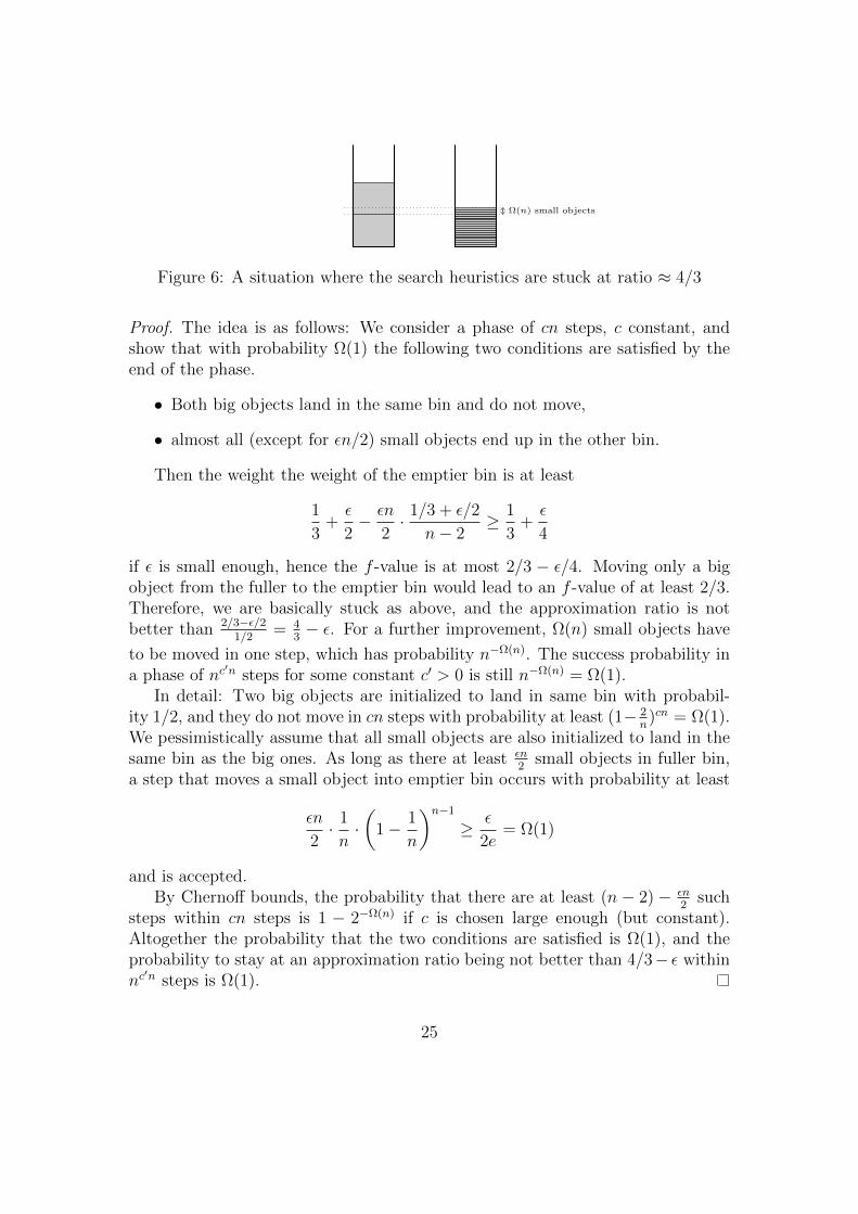
Ω(n) small objects

Figure 6: A situation where the search heuristics are stuck at ratio ≈ 4/3

Proof. The idea is as follows: We consider a phase of cn steps, c constant, andshow that with probability Ω(1) the following two conditions are satisfied by theend of the phase.

∙ Both big objects land in the same bin and do not move,

∙ almost all (except for �n/2) small objects end up in the other bin.

Then the weight the weight of the emptier bin is at least

1

3+�

2− �n

2⋅ 1/3 + �/2

n− 2≥ 1

3+�

4

if � is small enough, hence the f -value is at most 2/3 − �/4. Moving only a bigobject from the fuller to the emptier bin would lead to an f -value of at least 2/3.Therefore, we are basically stuck as above, and the approximation ratio is notbetter than 2/3−�/2

1/2= 4

3− �. For a further improvement, Ω(n) small objects have

to be moved in one step, which has probability n−Ω(n). The success probability ina phase of nc

′n steps for some constant c′ > 0 is still n−Ω(n) = Ω(1).In detail: Two big objects are initialized to land in same bin with probabil-

ity 1/2, and they do not move in cn steps with probability at least (1− 2n)cn = Ω(1).

We pessimistically assume that all small objects are also initialized to land in thesame bin as the big ones. As long as there at least �n

2small objects in fuller bin,

a step that moves a small object into emptier bin occurs with probability at least

�n

2⋅ 1

n⋅(

1− 1

n

)n−1

≥ �

2e= Ω(1)

and is accepted.By Chernoff bounds, the probability that there are at least (n − 2) − �n

2such

steps within cn steps is 1 − 2−Ω(n) if c is chosen large enough (but constant).Altogether the probability that the two conditions are satisfied is Ω(1), and theprobability to stay at an approximation ratio being not better than 4/3− � withinnc′n steps is Ω(1).

25

6.3 Improving the Approximation Ratio

The previous worst-case result showed that it is important to handle big objectsin the instance correctly. In this subsection, we show that good approximationscan be found in this way.

The following theorem shows how (1 + �)-approximations can be obtained,where � is assumed constant. Actually, a more general statement, where � isallowed to converge to zero, can be shown, see Neumann and Witt (2010, page102) for details.

Theorem 17. Let � > 0 be an arbitrarily small constant. There are constantsc1, c2 > 0 such that RLS and the (1+1) EA on any instance find (1+�)-approximatesolutions with probability ≥ 2−c1/� in at most c2n/� steps.

Before we prove the theorem, we discuss how to interpret it. Even thougha success probability of 2−c1/� may sound small, it can be boosted by repeatingthe algorithm. After an expected number of 2c1/� repetitions we have achieved the(1+�)-approximation, and the expected total time is only 2c1/�c2n/� = O(n), since� is a constant.

Proof of Theorem 17. Let s := ⌈1/�⌉. By Lemma 7, we have pi ≤ P/s ≤ �P fori ≥ s. We call the objects of index at least s small, big otherwise (see Figure 7for an illustration). The idea is that if the algorithm moves small objects fromthe fuller into the emptier bin until no further improvements are possible, thenthe volume of the fuller bin is by at most �P/2 larger than in an optimal solution.This implies a (1 + �)-approximate solution.

p1 p2 p3 p4 p5 p6 p7 p8≤ �P

Figure 7: Division into big and small objects

We make these ideas precise. We consider an optimal distribution of the s− 1big objects to the two bins and denote by L∗ the volume of the fuller bin forthis optimal distribution. The probability that the big objects accord with theoptimal distribution in the initial search point is at least 2−s+1 ≥ 2−1/� since theinitial search point is drawn uniformly. After initialization, we consider a phase

26

consisting of t := c2n/� steps. The probability that none of the big objects movesin this phase is at least (

1− s− 1

n

)c2n/�= 2−Ω(1/�).

It remains to show that a sufficient number of small objects is distributed. We callthe phase successful if the approximation ratio at its end is (1 + �).

Using the usual argumentation on sufficient conditions for progress, the al-gorithm can make improvements by moving small objects from the fuller to theemptier bin as long as the f -value is greater than max{P/2, L∗}+ �P/2 (assumingthe big objects to be fixed). We estimate the contribution of small objects tothe fuller bin using the method of expected multiplicative distance decrease fromTheorem 10. We define Dt := f(x)− P/2, hence Dt measures the contribution ofsmall objects to the fuller bin. When the f -value is at most max{P/2, L∗}+ �P/2,we stop our considerations. It holds

E(Dt+1 ∣ Dt = d) ≤ d ⋅(

1− 1

en

)since moving small objects from the fuller to the emptier bin using single-bit flips ofprobability at least 1/(en) decreases the f -value until we stop the considerations.The expected contribution after t steps is at most ≤ P (1 − 1

en)c2n/�, which is less

than �P/4 if c2 is large enough. Using Markov’s inequality, the contribution aftert steps is at most �P/2 with probability at least 1/2. Altogether, the phase issuccessful with probability at least 2−1/� ⋅ 2−Ω(1/�) ⋅ (1/2) = 2−Ω(1/�).

6.4 An Average-Case Analysis

All analyses so far were dealing with arbitrary inputs to the problem, so thatthey implicitly also considered the worst-case input. From the viewpoint of apractitioner running the algorithm, this worst-case model analysis might be overlypessimistic. In practice, the worst-case inputs studied might be rare not even occurat all.

A common alternative is average-case models. A classical example for thebenefits of average-case models is given by simple deterministic Quicksort imple-mentations. These might take Ω(n2) steps in the worst case, e. g., if the input isthe reverse of the sorted sequence. If the sequence is assumed uniform at randomover all permutations, then the expected runtime of Quicksort is only O(n log n).It should be noted that average-case analyses assume a probability distributionover the sets of possible inputs.

27

The distribution that we consider in this subsection is very simple. We assumethat each weight pi is drawn uniformly and independently from [0, 1]. We call ouraverage-case model the uniform-distribution model. Despite the simplicity of themodel, the analysis of randomized search heuristics will be challenging. The reasonis that we are confronted with two sources of randomness, namely a randomizedalgorithm on a random input.

In this section, we do not longer consider the approximation ratio obtained bythe heuristic since it is not clear how to define this measure for random inputs.Instead, one typically considers the discrepancy,

d(x) :=

∣∣∣∣∣n∑i=1

pixi −n∑i=1

pi(1− xi)

∣∣∣∣∣,i. e., the absolute difference of weights of the bins and asks how close to discrep-ancy 0 the search heuristics come within a certain time span.

We start by noting that the discrepancy of the initial search point is large.

Theorem 18. With probability Ω(1), the initial discrepancy of (1+1) EA and RLSin the uniform-distribution model is Ω(

√n).

Proof. Let N denote the number of objects assigned to the first bin by the initialsearch point. Obviously, N is binomially distributed with parameters n and 1/2.A standard result from probability yields that Prob(N > n/2+

√n) = Ω(1), which

is due to the variance of the binomial distribution.Now let Si denote the sum of weights in bin i. Since each weight is uniform

over [0, 1] with expectation 1/2, we obtain E(S1) = N/2 and E(S2) = (n−N)/2.Moreover, the Si are symmetrical around the expectation, i. e., Prob(Si > E(Si)) =Prob(Si < E(Si)) since the single terms of the sum are symmetrical distributions.Moreover, Prob(Si = E(Si)) = 0 by the properties of the uniform distribution.We finally obtain Prob(S1 > E(S1) ∧ S2 < E(S2)) = 1/4.

Altogether, we have with probability Ω(1) that S1 > n/4 +√n/2 and S2 <

n/4−√n/2, hence the discrepancy is at least

√n with probability Ω(1).

It is not too difficult to see that RLS and the (1+1) EA reduce the discrepancyto at most 1 in an expected number of O(n2) steps. The following theorem showsthat significantly smaller discrepancies will be obtained in polynomial time withhigh probability. Actually, the discrepancy described by the theorem convergesto 0 with growing n

Theorem 19. After O(n5 log n) steps, the discrepancy of the (1+1) EA in theuniform-distribution model is at most O((log n)/n) with probability at least 1 −O(1/n).

28

It should be noted that the theorem does not include RLS.

Idea of proof. One important idea is to consider swaps of objects. If object i is inthe fuller bin, object j in the emptier one, and if the discrepancy is greater than2(pi− pj) > 0, then the objects can be swapped, resulting in that the discrepancydecreases by 2(pi−pj). More generally, we can consider so-called difference objectsmade from an object in the fuller bin and a smaller object in the emptier bin, suchthat the size of the difference object is the difference of the two objects. In thefollowing, we will show that with probability 1−O(1/n) there is always a differenceobject of size O((log n)/n). Then the usual arguments on local progress can beapplied.

To show the statement on the difference jobs, we consider the order statisticsof the n objects. Let X(i) denote the object of rank i among the n random objects,i. e., X(1) is the maximum and X(n) the minimum. For the uniform-distributionmodel, the distribution of the order statistics are well known, and we will exploitthe property

Prob(X(i) −X(i+1) ≥ t) = Prob(X(n) ≥ t) = (1− t)n. (1)

Choosing t∗ = (2 lnn)/n, we obtain (1 − t∗)n ≤ 1/n2. Hence, with probability atleast 1− 1/n (union bound), it holds that X(i) −X(i+1) ≤ t∗ for all 1 ≤ i ≤ n− 1and also X(n) ≤ t∗. In the following, we assume that this has happened.

It is an exercise to show that at any time, at least one of the following twoholds:

∙ For at least one i, the object of rank i is in the fuller and the object ofrank i+ 1 is in the emptier bin.

∙ The object of rank n is in the fuller bin.

Hence, as long as the discrepancy is greather than 2t∗ = O(log n/n), there is aswap of objects or a movement of the minimum object such that the discrepancy isreduced. The amount of improvement is determined by the smallest of X(i)−X(i+1)

and X(n). Using (1) once again, we can prove that X(i) − X(i+1) ≥ 2/n3 for1 ≤ i ≤ n − 1 and X(n) ≥ 2/n3 all hold with probability at least 1 − O(1/n).Assumings this to happen, the discrepancy is reduced by at least 2/n3 in everystep (if it is greater than 2t∗) with probability at least 1/(en2) since a 2-bit flip issufficient.

We can assume to start with discrepancy at most 1 since this is guaranteedafter an expected number of at most O(n2) steps. As argued in the precedingparagraph, the expected time to reduce the discrepancy from 1 to at most 2t∗ isat most c′n5 for some constant c′, and it is bounded by 2c′n5 with probablity atleast 1/2 using Markov’s inequality. If the goal is not reached within a phase of

29

2c′n5 steps, the probability of reaching it within the next 2c′n5 steps is again atleast 1/2. Altogether, the probability of not reaching the goal within log n phasesconsisting of 2c′n5 steps each is at most (1/2)logn, which means that the goal isreached within 2c′n5 log n = O(n5 log n) steps with probability at least 1 − 1/n.The sum of all failure probabilities is O(1/n).

The result of Theorem 19 is encouraging since it shows that randomized searchheuristics can obtain very good solutions in average-case models for NP-hard prob-lems. It is an important direction for future research to carry out further average-case analyses of simple randomized search heuristics.

7 Simulated Annealing vs. Metropolis

The previous sections were concerned with the (1+1) EA, i. e., a simple evolution-ary algorithm, and randomized local search. In this final part, we will considerone of the oldest randomized search heuristics, namely the Metropolis Algorithm(invented in 1953) and Simulated Annealing, see Algorithms 3 and 4, respectively.The mutation step is as in RLS since exactly one bit is chosen to flip. However,the selection is not strict in the sense that only search points with at least thesame fitness (assuming a maximization problem) as before are accepted. If thenew search point y has inferior fitness, it is possibly accepted anyway. In this way,the algorithm has the ability to escape from local optima, where RLS might bestuck.

Algorithm 3 Metropolis Algorithm (MA) for maximization


2. y := x

3. Choose one bit in y uniformly at random and flip it.

4. If f(y) ≥ f(x) Then x := y; Else x := y with probability e(f(y)−f(x))/T , whereT is fixed.


The probability to acccept worsenings depends on the fitness difference f(y)−f(x) < 0 from the previous search point and the parameter Tt (or just T ), calledtemperature. The larger Tt and the smaller ∣f(y)−f(x)∣, the larger the probabilityof accepting a worsening. If Tt > 0, the probability is certainly positive, while Tt =

30

Algorithm 4 Simulated Annealing (SA) for maximization


2. y := x


4. If f(y) ≥ f(x) Then x := y; Else x := y with probability e(f(y)−f(x))/Tt , whereTt may depend on t.


0 implies that a worsening is accepted with probability e(f(y)−f(x))/0 = e−∞ = 0.Hence, RLS is a special case of MA. Moreover, the only distinguishing feature ofMA and SA is the choice of Tt. In MA, T = Tt is not allowed to depend on the timeindex, which means that the algorithm has to work with a fixed temperature inall time steps. In SA, the temperature is allowed to depend on time, and typicallyTt decreases in a certain way with t, which is called cooling schedule. The reasonis that the first steps of the heuristic should follow a more chaotic behavior andbe able to jump around in the search space to leave local optima, while the latersteps should fine-tune the search process in a region of high fitness such that nodrastic worsenings should happen any longer. The nature-inspired idea is relatedto annealing of crystals, which follows also a kind of “cooling down” to arrive at acertain shape of the crystal.

For a long time, there was no illustrative example that showed the benefitsof SA compared to MA, more precisely there was no proof that a well-chosencooling schedule could decrease the runtime of SA compared to MA on a prob-lem from combinatorial optimization. This open problem was solved by Wegener(2005). Actually, the example he presented does not allow efficient optimizationwith MA at any temperature. The cooling schedule by SA is simple and allows forpolynomial runtimes. In this section, we describe the example where “simulatedannealing beats metropolis in combinatorial optimization” in detail along withnew interesting and important techniques for the analysis of randomized searchheuristics.

7.1 A Minimum Spanning Tree Instance

It turns out that SA beats MA on a simple instance to the minimum spanningtree (MST) problem defined in Section 4. To keep things simple, we let the searchheuristic start with the all-ones string instead of a uniformly random string. This

31

corresponds to the case that all edges have been chosen, hence the subgraph en-coded by the all-ones string is connected. We avoid the complicated penalty termsfrom Section 4 and give unconnected graphs just an infinite f -value. More pre-cisely, as before we let x ∈ {0, 1}n encode a subset E ′ ⊆ E of the edge set of theunderlying weighted graph G = (V,E,w) and define

f(x) :=

{total cost of E ′ if (V,E ′) is a connected graph,

∞ otherwise.

The aim is to minimize f , which leads to the search heuristic given as Algorithm 5.If Tt does not depend on t, we call the heuristic MA, otherwise we call it SA.

Algorithm 5 SA/MA for minimization


2. y := x


4. If f(y) ≤ f(x) Then x := y; Else x := y with probability e(f(x)−f(y))/Tt .


We now define the instance to the MST problem where SA beats MA. Letn = 6k. Similarly to the example from Section 4.3, the instance considered hereconsists of n/3 connected triangles, half of which are called light and half of whichare called heavy. Each triangle has two light edges and one heavy edge. The edgesin the light triangles have weight 1 and n, while the edges in the heavy triangleshave weight n2 and n3. Hence, a heavy edge in a light triangle is still much lighterthan a light edge in a heavy triangle. Obviously, the minimum spanning tree isunique and consists of light edges, only. See Figure 8 for an illustration.

n

11

n

11

n

11

n

11

n3

n2n2

n3

n2n2

n3

n2n2

n3

n2n2

Figure 8: The MST instance where SA beats MA

The aim is to show that MA with arbitrary fixed temperature T typically needsexponential time on the instance, whereas SA with an appropriate cooling scheduletypically finds optimum in polynomial time. The basic idea is that temporary

32

worsenings of the f -value are necessary during the optimization process to correcttriangles, and that this requires two different temperatures. On the one hand,if the temperature is low, the algorithm is unlikely to correct mistakes made atheavy triangles. On the other hand, if the temperature is high, the search processat the light triangles is too chaotic and it is likely to destroy correct light trianglesagain. If the temperature is decreased slowly, though, then the search process canfirst correct the heavy triangles at high temperature and then the light trianglesat low temperature.

7.2 Lower Bound for MA

The aim is to show the following theorem, which shows that MA is highly inefficenton the chosen instance, regardless of the temperature.

Theorem 20. The probability that MA with arbitrary but fixed T computes theMST within ecn steps (c a small enough positive constant) is bounded from aboveby e−Ω(n).

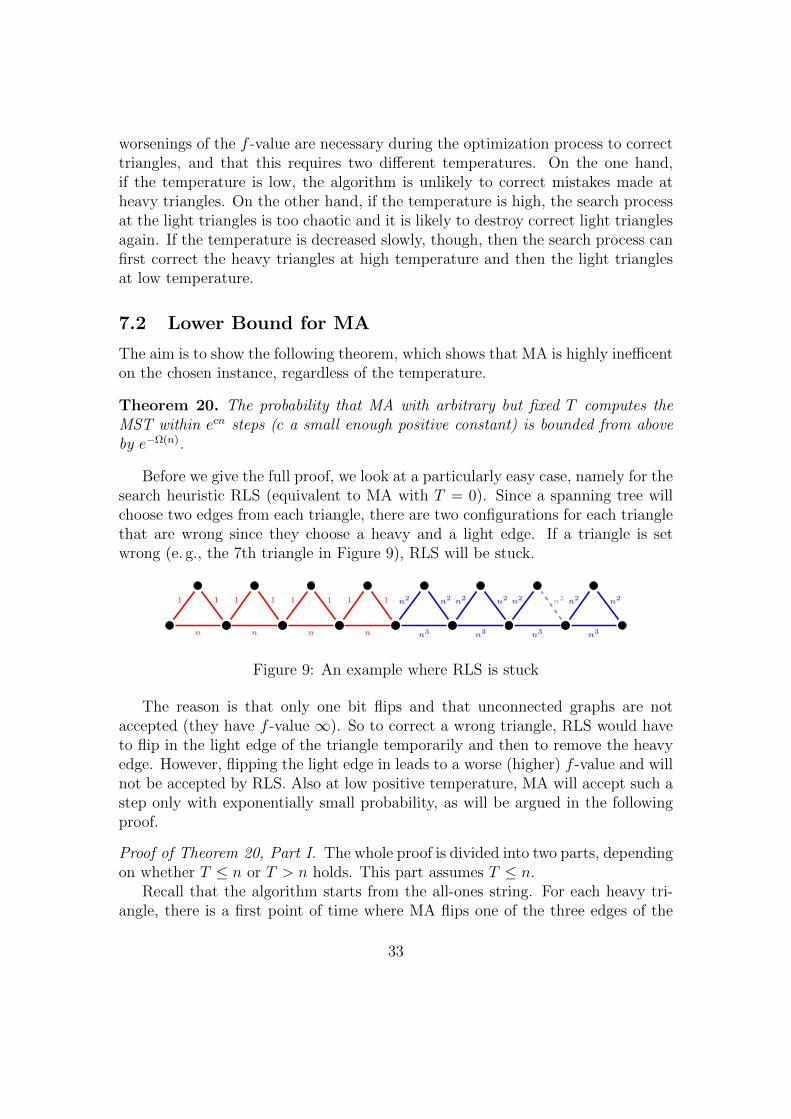
Before we give the full proof, we look at a particularly easy case, namely for thesearch heuristic RLS (equivalent to MA with T = 0). Since a spanning tree willchoose two edges from each triangle, there are two configurations for each trianglethat are wrong since they choose a heavy and a light edge. If a triangle is setwrong (e. g., the 7th triangle in Figure 9), RLS will be stuck.

n

11

n

11

n

11

n

11

n3

n2n2

n3

n2n2

n3

n2n2

n3

n2n2

Figure 9: An example where RLS is stuck

The reason is that only one bit flips and that unconnected graphs are notaccepted (they have f -value ∞). So to correct a wrong triangle, RLS would haveto flip in the light edge of the triangle temporarily and then to remove the heavyedge. However, flipping the light edge in leads to a worse (higher) f -value and willnot be accepted by RLS. Also at low positive temperature, MA will accept such astep only with exponentially small probability, as will be argued in the followingproof.

Proof of Theorem 20, Part I. The whole proof is divided into two parts, dependingon whether T ≤ n or T > n holds. This part assumes T ≤ n.

Recall that the algorithm starts from the all-ones string. For each heavy tri-angle, there is a first point of time where MA flips one of the three edges of the

33

triangle. With probability only 1/3, the step flips a heavy edge, i. e., a light edgeis excluded from the triangle with probability 2/3. The probability that these firststeps exclude the heavy edges from all heavy triangles is only (1/3)n/6 = 2−Ω(n).Consequently, with probablity 1−2−Ω(n) there is after some time at least one heavytriangle that is configured wrongly and missing a light edge.

As argued above, to correct a wrong triangle it is necessary to temporarilyflip in a light edge before exluding the heavy edge. Let x be a search point witha wrong heavy triangle. A step that flips in the light edge will lead to a searchpoint y with f(y) = f(x)+n2 due to the weight of a light edge in a heavy triangle.Hence, y is accepted as a new search point only with probability e−n

2/T ≤ e−n

since T ≤ n. The probability that such step is accepted within en/2 steps is atmost en/2 ⋅ e−n = e−n/2 = 2−Ω(n) by the union bound. Hence, altogether withprobability 1− 2−Ω(n), the MST will not be found within en/2 steps.

We are left with the case T > n. As said above, a high temperature makes thesearch process more chaotic and leads to frequent acceptance of worsenings. Withrespect to the light triangles, it will often happen that steps are accepted that flipan unnecessary edge in again. More precisely, we distinguish for each triangle 1correct, 2 wrong and 1 complete configurations (see Figure 7.2 for an illustration).The aim is to show that the algorithm is inclined to prefer wrong and completeconfigurations towards the correct ones.

correct

n

11

wrongn

11

wrongn

11

n

11

complete

Formalizing this idea is more difficult. The algorithm tends to drift to incor-rect configurations of light triangles only if there are already many correct lighttriangles. This behavior can be covered by so-called drift analysis, which will bepresented as a general tool now. The negative drift theorem (Theorem 21) de-scribes the following scenario: A random process has to pass the interval [a, b]from “left to right”, and within the interval, it moves to the left in expectation(first condition of the theorem). Steps to the right direction are possible, but un-likely, and especially large jumps are extremely unlikely (second condition). SeeFigure 10 for an illustration. Intuition suggests that it takes a long time to passthe interval, which is formalized by the theorem. The random variable T ∗ denotesthe first point of time where position at least b is reached if the process startsat position at most a. Roughly, the theorem states that T ∗ is exponential in theinterval length with high probability.

34

Theorem 21 (Negative Drift Theorem). Let Xt, t ≥ 0, denote a stochastic processover S := {0, 1, . . . , N}. Denote Δt(i) := (Xt+1−Xt ∣ Xt = i) for i ∈ S and t ≥ 0.Suppose that there exists an interval [a, b] ⊆ S and three constants �, � > 0, � < 1such that for all t ≥ 0

1. E(Δt(i)) ≤ −� for a < i < b

2. Prob(Δt(i) = j) ≤ � ⋅ �j for i < b and j ≥ 1

then there is a constant c∗ > 0 such that for T ∗ := min{t ≥ 0: Xt ≥ b ∣ X0 ≤ a}it holds Prob(T ∗ ≤ 2c

∗(b−a)) = 2−Ω(b−a).

It should be noted that �, �, � must not depend on N (neither on a or b).

starta b

target

drift away from target

no large jumpstowards target

Figure 10: Illustration of Negative Drift Theorem

The negative drift theorem has many applications. In order to exercise its use,we present an application for an example problem before we proceed with the proofof Theorem 20.

Let us consider the function

Needle(x) =

{1 if x = (1, . . . , 1)

0 otherwise,

which has a unique optimum in the all-ones string, whereas all other search pointshave the same function value. The function thus consists of a huge plateau anddoes not give any hints on the optimum, which is a “needle in a haystack” of 2n

search points. It is intuitive that randomized search heuristics will not be efficienton Needle, which we formalize as follows.

Theorem 22. With probability 1− 2−Ω(n), RLS needs at least 2Ω(n) steps to opti-mize Needle.

Proof. The aim is to apply Theorem 21. We define the random variable Xt as thenumber of one-bits in RLS’s current search point at time t. Using the linearity ofexpectation and the fact that each bit is flipped with probability 1/n, it is easy tosee that a mutation flips an expected number of Xt

n1-bits and an expected number

of n−Xt

n0-bits. Except for Xt = n, the next search point created by mutation is

35

always accepted, which implies E(Xt+1 ∣ Xt) = Xt + n−Xt

n− Xt

n. In other words,

using the notation from Theorem 21, we have

E(Δt(i) ∣ Xt = i) =n− in− i

n=n− 2i

n,

which is negative for i > n/2. By choosing a := 23n and b := n (other values

would be possible), we get n−2in≤ −1/3 for i ≥ a, hence the first condition of the

negative drift theorem is satisfied by choosing � := −1/3.The second condition is trivial to fulfil by choosing � = 1/2 and � = 2. We

have Prob(Xt+1 = i+ j ∣ Xt = i) ≤ 2 ⋅(

12

)jfor j ≥ 1 since RLS flips only one bit.

Note that 2(

12

)j= 1 for j = 1.

Finally, by Chernoff bounds we have Prob(X0 ≤ 2n/3) = 1 − 2−Ω(n). Alto-gether, we obtain an optimization time of at least 2Ω(b−a) = 2Ω(n) with probaba-bility at least 1− 2−Ω(n) from the negative drift theorem.

We proceed with the proof of the lower bound for MA.

Proof of Theorem 20, Part II. We assume T > n. The aim is to apply the negativedrift theorem (Theorem 21) on the number of correct light triangles. Therefore, letXt denote the number of correct light triangles at time t and note that Xt ≤ n/6.Since MA initializes with the all-ones string, we also know that X0 = 0.

Since only one bits flips per step, it holds Xt+1 − Xt ∈ {−1, 0, 1}. Hence,using the same argument as in the proof of Theorem 22, the second conditionof the drift theorem is trivially satisfied with � = 1/2 and � = 2. With respectto the first condition, we introduce p+

i := Prob(Xt+1 = i + 1 ∣ Xt = i) andp−i := Prob(Xt+1 = i − 1 ∣ Xt = i) and note that E(Δt(i) ∣ Xt = i) = p+

i − p−i .Since it is necessary for an increase of Xt to flip out the heavy edge in one of then/6 − i wrong/complete triangles, we get p+

i ≤n/6−in

. Since it is sufficient for adecrease of Xt to flip in the heavy edge in one of i correct triangles and to acceptthe step, we get p−i ≥ i

n⋅ e−n/T ≥ i

n⋅ e−1 ≥ i

3n, where we have used that T ≥ n.

The drift interval contains the configurations with at least 90% and at most100% correct light triangles, i. e., a := 9

10⋅ n

6= 3n

20and b := n/6. This yields

E(Δt(i)) ≤ p+i − p−i = 1

60− 1

20= −1

30for i ≥ a, and the first condition of the

drift theorem is satisfied. Since we start with X0 = 0, and since Xt = n/6 isnecessary for an optimal search point, the negative drift theorem tells us that theoptimization time is 2Ω(b−a) = 2Ω(n) with probability at least 1− 2−Ω(n).

7.3 Upper Bound for SA

In this section, we show that SA is efficient on the considered MST instance. Thecooling schedule is Tt := n3 ⋅ (1− 1/(cn))t for some constant t, which means thatthe temperature starts at n3 and decreases to at most 1 within 3cn lnn steps.

36

Theorem 23. Choosing the cooling schedule Tt := n3 ⋅ (1− 1/(cn))t for some suf-ficiently large constant c > 0, SA computes the MST within 3cn lnn = O(n log n)steps with probability at least 1− 1

p(n), where p(n) is an arbitrary polynomial.

Proof. The proof idea is as follows: We concentrate on the phases where thetemperature is in the intervals [n2, n5/2] and [1, n1/2]. When it is in the firstinterval, the heavy triangles are corrected with high probability, whereas the lighttriangles are corrected with high probability when the temperature is in the secondinterval. We solve (1− 1/(cn))ℓ = n−1/2 to obtain that the number of steps spentin each interval is ℓ := −(1/2)(ln(n))/ln(1− 1/(cn)) ≈ (c/2)n lnn, where we haveused ln(1 − x) ≈ x for −x close to 0. Note that the approximation becomesmore and more precise with increasing n. If c is large enough, then coupon-collector-like processes correct wrong triangles with high probability. Steps wherethe temperature is outside the intervals do not harm with high probability. Finally,we note that T3cn lnn ≤ 1.

We make these ideas more precise. Let us consider the first phase, i. e., thepoints of time t such that Tt ∈ [n2, n5/2]. We only look at the heavy trianglesand distinguish as in Section 7.2 between correct, wrong and complete configura-tions. A possible bad behavior is that a step is accepted that flips the heavy edgeof an already correct triangle in again, i. e., makes a correct triangle complete.However, the probability that this occurs at some point of time in the phase isat most c

2(n lnn)e−n

3/Tt ≤ e−Ω(n1/2), using the union bound and Tt ≤ n5/2. Letus fix an arbitrary wrong or complete triangle. We would like the triangle tobe made correct. A sufficient condition for this is that the triangle is first madecomplete (if the triangle was not complete yet) and that the heavy edge is flippedout afterwards. We concentrate on the steps that affect the considered triangle,i. e., consider only steps that flip one of the three edges of the triangle. Withprobability (1/3) ⋅ e−n2/Tt ≥ e−1/3 (since Tt ≥ n2), such a step flips in the lightedge (if applicable) and is accepted, and with probability 1/3 it flips out the heavyedge. Two consecutive steps that affect the triangle are therefore correcting withprobability at least (e−1/3) ⋅ (1/3) ≥ 1/27. We now concentrate on pairs of stepsthat affect the considered triangle and remark that there might be many otherirrelevant steps in between these steps.

We have to show that the phases contains enough steps affecting a triangle toensure a total failure probability that is sufficiently small. If n is large enough,then the phase length ℓ satisfies ℓ ≥ (c/3)n lnn. We fix an edge e. The numberof times among ℓ steps where e is flipped is at least (c/4) lnn with probability atleast 1 − e−Ω(c lnn) = 1 − nΩ(c) according to Chernoff bounds. Given an arbitrarypolynomial p(n), for large enough but constant c the probability is at least 1− 1

8p(n).

We consider (c/8)n lnn pairs of steps, each of which is correcting with probabilityat least 1/27 as argued above. The probability of not correcting all heavy triangles

37

within the first phase is at most

n

6⋅(

26

27

)(c/8) lnn

≤ 1

8p(n)

for appropriate c. Altogether, by summing up all probabilities for failures, the firstphase is not successful with probability at most 1

8p(n)+ 1

8p(n)+ e−Ω(n−1/2) ≤ 1

3p(n).

For the second phase, a very similar analysis applies. The weights of the edgesof light triangles are by a factor of n2 smaller than for the heavy triangles, as is thetemperature in the phase. Using the same calculations, it follows that the secondphase corrects all light triangles with probability at least 1− 1

3p(n). The only prob-

lem that might occur is that a correct heavy triangle becomes wrong or completewithin the second phase again. However, the probability of this happening is atmost (c/2)n(lnn) ⋅ e−n2/Tt = e−Ω(n−3/2) since Tt ≤ n1/2.

The sum of all failure probablities is at most 1p(n)

if n is large enough, whichcompletes the proof.

7.4 SA vs. MA for TSP

The technique behind the MST example can be transferred to instances of NP-hardproblems. Meer (2007) considers the Traveling Salesperson Problem (TSP): Givena complete graph on the vertex set V = {1, . . . , n} and edge costs c(i, j) ∈ ℝ+, finda permutation � on the set {1, . . . , n} resulting in a Hamiltonian circuit (roundtrip, also called tour) of minimum total cost. The example instance he uses ismade up of the skeleton graph displayed in Figure 11, which takes the role of thetriangles from the MST instance.

3

1 2

4

65

Figure 11: The skeleton graph for the TSP instance

The edges that are drawn are called permissible. Those that are not drawn areassumed to have a huge cost such that they will never be chosen in the tours thatwe consider. More precisely, we will only consider tours that enter the skeleton ateither vertex 1 or vertex 6 and leave it at the other vertex from {1, 6}. The edge{1, 3} will be the heaviest edge in the skeleton, {1, 2} will be second-heaviest and

38

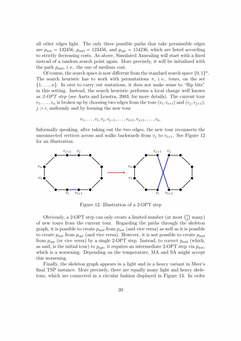
all other edges light. The only three possible paths that take permissible edgesare pwst = 132456, pmid = 123456, and popt = 154236, which are listed accordingto strictly decreasing costs. As above, Simulated Annealing will start with a fixedinstead of a random search point again. More precisely, it will be initialized withthe path pmid, i. e., the one of medium cost.

Of course, the search space is now different from the standard search space {0, 1}n.The search heuristic has to work with permutations �, i. e., tours, on the set{1, . . . , n}. In orer to carry out mutations, it does not make sense to “flip bits”in this setting. Instead, the search heuristic performs a local change well knownas 2-OPT step (see Aarts and Lenstra, 2003, for more details). The current tourv1, . . . , vn is broken up by choosing two edges from the tour (vi, vi+1) and (vj, vj+1),j > i, uniformly and by forming the new tour

v1, . . . , vi, vj, vj−1, . . . , vi+1, vj+1, . . . , vn.

Informally speaking, after taking out the two edges, the new tour reconnects theunconnected vertices across and walks backwards from vj to vi+1. See Figure 12for an illustration.

v1

vn

vj+1 vj

vi+1vi

v1

vn

vj+1 vj

vi+1vi

Figure 12: Illustration of a 2-OPT step

Obviously, a 2-OPT step can only create a limited number (at most(n2

)many)

of new tours from the current tour. Regarding the paths through the skeletongraph, it is possible to create pmid from pwst (and vice versa) as well as it is possibleto create pwst from popt (and vice versa). However, it is not possible to create pmid

from popt (or vice versa) by a single 2-OPT step. Instead, to correct pmid (which,as said, is the initial tour) to popt, it requires an intermediate 2-OPT step via pwst,which is a worsening. Depending on the temperature, MA and SA might acceptthis worsening.

Finally, the skeleton graph appears in a light and in a heavy variant in Meer’sfinal TSP instance. More precisely, there are equally many light and heavy skele-tons, which are connected in a circular fashion displayed in Figure 13. In order

39

to find the optimal tour, the subtours through all skeleton graphs have to be cor-rected at least once. The ideas worked out above for the MST instance apply:MA with fixed temperature fails either at the heavy or light skeletons, while SAwith an appropriate cooling schedule will optimize heavy and light skeletons oneafter another. The detailed analysis uses the same techniques as above, and theinterested reader is referred to Meer (2007) for the full proof.

heavy heavy heavy heavy

light light light light

Figure 13: A sketch of the whole TSP instance

References

Aarts, Emile and Lenstra, Jan Karel (2003). Local Search in Combinatorial Opti-mization. Princeton University Press.

Droste, S., Jansen, T., and Wegener, I. (2002). On the analysis of the (1+1)evolutionary algorithm. Theoretical Computer Science, 276, 51–81.

Feller, W. (1968). An Introduction to Probability Theory and Its Applications,vol. 1. Wiley, 3rd ed.

Garey, M. and Johnson, D. S. (1979). Computers and Intractability: A Guide tothe Theory of NP-Completeness. W.H. Freeman and Company.

Hochbaum, D. (1997). Appromixation Algorithms for NP-hard Problems. PWSPublishing Company.

Hopcroft, J. E. and Karp, R. M. (1973). An n5/2 algorithm for maximum matchingsin bipartite graphs. SIAM Journal on Computing, 2, 225–231.

Mayr, Ernst W. and Plaxton, C. Greg (1992). On the spanning trees of weightedgraphs. Combinatorica, 12(4), 433–447.

Meer, Klaus (2007). Simulated Annealing versus Metropolis for a TSP instance.Information Processing Letters, 104(6), 216–219.

40

Motwani, R. and Raghavan, P. (1995). Randomized Algorithms. Cambridge Uni-versity Press.

Neumann, F. and Witt, C. (2010). Bioinspired Computation in Combinatorial Op-timization – Algorithms and Their Computational Complexity. Springer. Onlineversion available on www.bioinspiredcomputation.com.

Wegener, I. (2005). Simulated annealing beats Metropolis in combinatorial opti-mization. In Proceedings of the 32nd International Colloquium on Automata,Languages and Programming (ICALP ’05), vol. 3580 of Lecture Notes on Com-puter Science, 589–601. Springer.

41

A Appendix

In this appendix, we list definitions and results from probability theory that will beneeded to analyze randomized search heuristics. These will be described withouttoo much formalism if this can be avoided. Having said that, the material assumesthe reader to be familiar with discrete event spaces, probabilities and expectedvalues. Moreover, the O-notation should be known. By log(n) we denote thebinary logarithm (base 2) and by ln(n) the natural logarithm (base e).

The following notions are fundamental:

∙ An event is (a set of) something that can happen or not happen

∙ A random variable X maps outcomes of events to valuesExample: roll a die → X ∈ {1, . . . , 6}

∙ By Prob(A) we denote the probability of event AExample: Prob(die shows 6) = 1/6

∙ By E(X) we denote the expected value of XExample E(X) = 1

6(1 + 2 + 3 + 4 + 5 + 6) = 3.5

∙ By Prob(A ∣ B) we denote the conditional probability of event A givenevent B. By E(X ∣ B) we denote the conditional expectation of X givenevent B.

∙ Sequences of random variables Xt, t ≥ 0: model stochastic processExample: Xt current bitstring of (1+1) EA in step t

∙ A Markov chain is a stochastic process satisfying : (Xt+1 ∣ Xt, Xt−1, . . . , X0) =(Xt+1 ∣ Xt), hence only most recent state influences the next one

The following list allow us to manipulate expected values, defines the notion ofstochastic independence and states a simple bound on the probability of a unionof events.

∙ Linearity of expectation: E(X + Y ) = E(X) + E(Y ) for arbitrary X, Y

∙ Law of total probability:Prob(A) =

∑ni=1 Prob(A ∣ Bi) ⋅ Prob(Bi)

for a partition B1, . . . , Bn of the space of all events

∙ The law of total probability for expected values:E(X) =

∑ni=1E(X ∣ Bi) ⋅ Prob(Bi)

42

∙ Events A,B (random variables X, Y ) are independent ifProb(A ∩B) = Prob(A) ⋅ Prob(B) (E(X ⋅ Y ) = E(X) ⋅ E(Y ))

∙ Union bound: Prob(A ∪B) ≤ Prob(A) + Prob(B)

The expected value of a random variable is an average value that does not tellmuch about the real distribution of the variable in general. Under certain circum-stances, however, random variables typically take values close to their expectationand are called sharply concentrated then. The following so-called concentrationinequalities cover such cases.

∙ Markov’s inequality : If X is a random variable with non-negative outcomesthen Prob(X ≥ t ⋅ E(X)) ≤ 1

tfor any t.

Example: algorithm with expected runtime n2 does not finish in time n3

with probability ≤ 1n.

∙ Chernoff’s inequality : Let X1, . . . , Xn be independent {0, 1}-random vari-ables with pi := Prob(Xi = 1), 1 ≤ i ≤ n. For X :=

∑ni=1Xi and

� := E(X) =∑n

i=1 pi we have

1. Prob(X < (1− �)�) < e−��2/2 for 0 < � < 1,

2. Prob(X > (1 + �)�) < e−��2/3 for 0 < � < 1.

Toy example: Assume a fair coin is tossed n times. Then Xi, 1 ≤ i ≤ n, isdefined to be 1 iff the outcome is heads in the i-th trial. We can apply Cher-noff bounds on X = X1+⋅ ⋅ ⋅+Xn using � = n/2 and � = 1/5 and obtain thatthe number of heads among 1000 toin cosses is in [400, 600] with probability≥ 0.997. If the coin is tossed 10000 times, then the number of heads is in[4000, 6000] with probability ≥ 0.99999999999999999999999999992. That is,Chernoff bounds tend to become more powerful with larger expected values.

A “serious application” of Chernoff bounds applies to the number of 1-bitsin a uniform bit string of length n, which is typically used as the initialsolution in randomized search heuristics. Each bit is set to 1 independentlywith probability 1/2, hence Chernoff bounds can be applied. They yield thatthe number of 1-bits is in [1

3n, 2

3n] with prob. 1− 2−Ω(n).

Finally, we list some commonly used inequalities, in particular about bit-flipprobabilities in the (1+1) EA and a result on the waiting time for certain events.For n ≥ k ≥ 1 it holds that

∙ lnn ≤∑n

i=11i≤ (lnn) + 1 (the sum is sometimes called the n-th Harmonic

number).

43

∙(1− 1

n

)n−1 ≥ 1e≥(1− 1

n

)n(where e = 2.718...)

∙ nk

kk≤(nk

)≤ nk

k!

∙ Definition: For x = (x1, . . . , xn), y = (y1, . . . , yn) ∈ {0, 1}n we define theHamming distance H(x, y) :=

∑ni=1∣xi − yi∣; hence, the Hamming distance

yields the number of mismatched bits.

∙ The probability of mutating x to y by the standard mutation of the (1+1) EA

equals(

1n

)H(x,y) (1− 1

n

)n−H(x,y).

∙ Prob(step of (1+1) EA flips k specific bits) =(1n

)k (1− 1

n

)n−k ≥ 1enk

∙ Prob(step of (1+1) EA flips k arbitrary bits) =(nk

) (1n

)k (1− 1

n

)n−k ≥ nk

kk⋅ 1nk ⋅ 1

e= 1

ekk

Lemma 8 (Waiting time lemma). Assume that event A occurs in each step of asearch heuristic independently with prob. p. Then it holds that the expected firsttime until A occurs is at most 1/p.

Example: The expected number of steps until specific k bits flip is O(nk).

44

course 02283, f2011, lecture notes on randomized search heuristics

Documents