Distributed noise-shaping quantization: I. Beta duals of finite

frames and near-optimal quantization of random measurements

Evan Chou∗and C. Sinan Gunturk†

Courant Institute, NYU

submitted: May 18, 2014, last revised: Feb 24, 2016

Abstract

This paper introduces a new algorithm for the so-called “Analysis Problem” in quantizationof finite frame representations which provides a near-optimal solution in the case of random mea-surements. The main contributions include the development of a general quantization frameworkcalled distributed noise-shaping, and in particular, beta duals of frames, as well as the perfor-mance analysis of beta duals in both deterministic and probabilistic settings. It is shown thatfor random frames, using beta duals results in near-optimally accurate reconstructions withrespect to both the frame redundancy and the number of levels that the frame coefficients arequantized at. More specifically, for any frame E of m vectors in Rk except possibly from asubset of Gaussian measure exponentially small in m and for any number L ≥ 2 of quantizationlevels per measurement to be used to encode the unit ball in Rk, there is an algorithmic quan-tization scheme and a dual frame together which guarantee a reconstruction error of at most√kL−(1−η)m/k, where η can be arbitrarily small for sufficiently large problems. Additional fea-

tures of the proposed algorithm include low computational cost and parallel implementability.

Keywords Finite frames, quantization, random matrices, noise shaping, beta encoding.

Mathematics Subject Classification 41A29, 94A29, 94A20, 42C15, 15B52

1 Introduction

Let X denote a bounded subset of Rk, such as the unit ball Bk2 with respect to the `2-norm, and A

denote a quantization alphabet (a finite subset of R), such as an arithmetic progression. Given afinite frame, i.e., a list of m vectors F := f1, . . . , fm that span Rk, we consider

Ds(F,A,X) := supx∈X

infq∈Am

∥∥∥∥∥x−m∑i=1

qifi

∥∥∥∥∥2

(1)

which represents the smallest error of approximation that can be attained uniformly over X byconsidering linear combinations of elements of F with coefficients in A. We will call this quantity

∗Current affiliation: Google New York. email: chou@cims.nyu.edu†Address: Courant Institute, 251 Mercer Street, New York, NY 10012. email: gunturk@cims.nyu.edu

1

arX

iv:1

405.

4628

v2 [

cs.I

T]

5 M

ay 2

016

the synthesis distortion associated with (F,A,X) (hence the subscript ‘s’). Understanding thenature of the synthesis distortion and finding quantization algorithms (i.e., maps x ∈ X 7→ q ∈ Am)that achieve or even approximate this quantity is generally an open problem, usually referred to asthe “Synthesis Problem” in the theory of quantization of frame representations [26].

The synthesis distortion can be seen as a generalized notion of linear discrepancy [18, 24]. Recall(e.g. [6, 23]) that the linear discrepancy of a k ×m matrix Φ is defined as

lindisc(Φ) := supy∈[−1,1]m

infq∈−1,1m

‖Φ(y − q)‖∞. (2)

We may define lindiscp(Φ) by replacing the∞-norm in (2) with any p-norm, 1 ≤ p ≤ ∞. We wouldthen have

lindisc2(F ) = Ds(F, −1, 1, F ([−1, 1]m)),

where F also stands for the matrix whose columns are (fi)m1 .

Consider any other frame E := e1, . . . , em in Rk that is dual to F , i.e.

m∑i=1

〈x, ei〉fi = x for all x ∈ Rk. (3)

We will write E for the matrix whose rows are (e>i )m1 . (Depending on the role it assumes, E willbe called the analysis frame or the sampling operator, and similarly F will be called the synthesisframe or the reconstruction operator.) It is then evident that (3) is equivalent to FE = I and alsothat duality of frames is a symmetric relation. We define the analysis distortion associated with(E,A,X) by

Da(E,A,X) := infDs(F,A,X) : FE = I. (4)

The analysis distortion has the following interpretation: Given an analysis frame E, the encoderchooses a quantization map Q : Rm → Am and the decoder chooses a synthesis frame F that isdual to E. The encoder maps each x ∈ X (or equivalently, the measurement vector y := Ex) toits quantized version q := Q(Ex), and using q the decoder produces Fq as its approximation tox. The optimal choice of Q and F (dual to E) yields the analysis distortion. We will refer to thisoptimization problem as the “Analysis Problem”. (Also see [26].)

There are some remarks to be made regarding the definition of the analysis distortion and itsabove interpretation:

First, the assumption that the reconstruction must be “linear” is made for practical reasons.Non-linear methods (such as consistent reconstruction [29, 15]) have also been considered in the lit-erature for the above type of encoders, but these methods generally come with higher computationalcost.

Second, the assumption that F be dual to E is made so that the reconstruction is guaranteedto be exact in the high-resolution quantization limit, or simply when there is no quantization. Itshould be noted that this assumption is also meaningful in order to make sense of how the choiceof E might influence the reconstruction accuracy: without any assumptions on F or Q, F can bechosen optimally (in the sense of minimizing the synthesis distortion for X) and Q can be chosento produce the corresponding optimally quantized coefficients, thereby erasing the influence of E.

To make these points more precise, let us define, for any pair of frames (E,F ) (not necessarilydual to each other) and any quantization map Q : Rm → Am,

D(E,Q, F,X) := supx∈X‖x− FQ(Ex)‖2. (5)

2

With this definition, we trivially obtain D(E,Q, F,X) ≥ Ds(F,A,X) so that

infQ

D(E,Q, F,X) ≥ Ds(F,A,X). (6)

In fact, (6) is an equality. To see this, note that the infimum in (1) is achieved for every x, so thereis an optimal q∗(x) ∈ Am that yields

Ds(F,A,X) = supx∈X‖x− Fq∗(x)‖2.

Since E is injective, a map Q∗ : Rm → Am can now be found such that Q∗(Ex) = q∗(x), whichthen yields

Ds(F,A,X) = D(E,Q∗, F,X) = infQ

D(E,Q, F,X).

This relation is valid for all E and F . Fixing E and minimizing over its dual frames F now resultsin the interpretation of the analysis distortion given in the previous paragraph:

Da(E,A,X) = inf(Q,F ):FE=I

D(E,Q, F,X). (7)

Finally, it should be noted that in the setup of this paper we do not allow the decoder to picka different linear map Fq depending on the quantized vector q that it receives. While such anadaptive method could be considered in practice, it would generally be classified as a non-lineardecoder.

The distortion performance of any given encoder-decoder scheme (adaptive or not) that uses atmost N codewords for X is constrained by the entropic lower bound ε(N,X) which is defined to bethe smallest ε > 0 for which there exists an ε-net1 for X of cardinality N . Then we have

D(E,Q, F,X) ≥ Ds(F,A,X) ≥ Da(E,A,X) ≥ ε(|A|m,X) (8)

where the second inequality assumes that FE = I. The entropic lower bound depends on A onlythrough its cardinality, so it will not necessarily be useful without a suitable matching between A

and X. For example, if the convex hull of F (Am) is small compared to X, then Ds(F,A,X) willbe artificially large. For the rest of this paper, we will fix X = Bk

2 . With slight abuse of notation,define

Ds(F,L) := infA:|A|=L

Ds(F,A, Bk2 ), (9)

andDa(E,L) := inf

A:|A|=LDa(E,A, B

k2 ). (10)

Since the cardinality N of any ε-net for Bk2 must satisfy the volumetric constraint Nvol(εBk

2 ) ≥vol(Bk

2 ), we have ε(N,Bk2 ) ≥ N−1/k. Hence, the relations in (8) and the definitions in (9) and (10)

yield, with N = Lm,Ds(F,L) ≥ Da(E,L) ≥ L−m/k.

One of the main results of this paper is a matching upper bound for the analysis distortion forGaussian random frames. We call E a standard Gaussian random frame if (Ei,j) are independentstandard Gaussian random variables.

1As is common, our convention for ε-nets is synonymous to ε-coverings: N is an ε-net for X if for all x ∈ X thereexists y ∈ N with ‖x− y‖2 ≤ ε.

3

Theorem 1.1. There exist absolute positive constants c1 and c2 such that for any scalar η ∈ (0, 1),if k ≥ 4

η and mk ≥

c1η2

log mk , then with probability at least 1 − exp(−c2η2m), a standard Gaussian

random frame E of m vectors in Rk satisfies

Da(E,L) ≤√kL−(1−η)m/k. (11)

for all L ≥ 2.

The proof of this theorem is constructive and algorithmic. Given η, we will, for each L, pro-vide a quantization alphabet A which is an arithmetic progression of size L, and an algorithmicquantization map Q : Rm → Am such that with high probability on E, there exists a certaindual frame F , determined by E and Q and computable by a fast, low-complexity algorithm, whichyields D(E,Q, F,Bk

2 ) . (m/k)3/2k−1L−(1−η)m/k. The chosen Q is a variation on vector-valuedβ-expansions and F is an alternative dual of E determined by Q. Suitably restricting the range ofm and k and summing over the failure probability for each L will then allow us to guarantee thedistortion bound (11) uniformly over L.

Quantization of finite frames by sigma-delta modulation goes back to [3, 2]. Alternative duals forframes were introduced in the context of sigma-delta quantization in [22, 21, 4], and more recentlyhave been effectively used for Gaussian random frames in [16] and more generally for sub-Gaussianrandom frames in [20]. For these frames, an r-th order sigma-delta quantization scheme coupledwith an associated Sobolev dual can achieve the bound Da(E,L) . L−1(cr)2r(m/k)−r with high

probability for some constant c. Optimizing this bound for r yields Da(E,L) . L−1e−c√m/k for

another constant c which is sub-optimal in terms of its dependence on both the alphabet size L andthe oversampling factor m/k and L. In contrast, our result achieves near-optimal dependence onboth parameters: Not only is the dependence on m/k exponential, but the rate can also be madearbitrarily close to its maximum value log2 L. To the best of our knowledge, this is the first resultof this kind.2

The paper is organized as follows: In Section 2, we review the notion of general noise-shapingquantizers and their stability as well as alternative duals of frames based on noise shaping. In thissection we introduce a number of new notions, namely, V -duals and V -condensation of frames andthe concept of distributed noise shaping. In Section 3, we introduce the special case of beta dualsand derive a general bound for the analysis distortion of an arbitrary frame using beta duals. Asan example, we show in this section that beta duals are optimal for harmonic semicircle frames. InSection 4, we bound the analysis distortion of Gaussian frames, prove Theorem 1.1 as well as somevariations of it, and also discuss the extension of our results to sub-Gaussian frames.

This paper is the first in a series of papers (in progress) on distributed noise shaping. Thefollow-up papers will address extensions of the theory developed in this paper for frames to moregeneral sampling scenarios, including compressive sampling and infinite dimensional systems.

2Similar exponential error bounds that have been obtained previously in the case of conventional sigma-deltamodulation or for other quantization schemes are not compatible with the results of this paper: The results of [17]and [11] are for a fixed frame-like system, but using a different norm in infinite dimensions, and the dependence onL is unavailable. The results in [12], obtained in yet another functional setting for sigma-delta modulation, comeclose to being optimal, however these results were obtained under modeling assumptions on the quantization noiseand circuit stability. The exponential near-entropic error decay in the bitrate obtained in [19] combine sigma-deltamodulation with further (lossy) bit encoding. Finally, the exponential error decay reported in [1] is obtained withadaptive hyperplane partitions and does not correspond to linear reconstruction.

4

2 Quantization via distributed noise shaping

2.1 Noise-shaping quantizers

Let A be a quantization alphabet and J be a compact interval in R. Let h = (hj)j≥0 be a givensequence, finite or infinite, and h0 = 1. By a noise-shaping quantizer with the transfer sequence h,we mean any map Q : Jm → Am where q := Q(y) satisfies

y − q = h ∗ u

and ‖u‖∞ ≤ C for some constant C which is independent of m. Here h∗u refers to the convolutionof h and u defined by (h ∗ u)n :=

∑hjun−j where it is assumed that un := 0 for n ≤ 0.

Noise-shaping refers to the fact that the “quantization noise” y − q cannot be arbitrary. Eventhough the operator H : u 7→ h ∗ u is invertible on Rm; the requirement that ‖u‖∞ must becontrolled uniformly in m imposes restrictions on what q can be for a given y.

The above formulation amounts to saying that H is an m×m lower triangular Toeplitz matrixdefined by h, in particular with unit diagonal. Let us relax the notion of a noise-shaping quantizerand assume that H is any given m ×m lower triangular matrix with unit diagonal. We will referto H as the noise transfer operator and keep the noise-shaping relation

y − q = Hu, (12)

but since H is more general and m is therefore static, we can no longer insist that ‖u‖∞ is controlledin the same manner. While we will mostly stick to convolution-based noise-shaping as defined atthe beginning, the above relaxation is conceptually and algebraically simpler.

Noise-shaping quantizers do not exist unconditionally. However, under certain suitable assump-tions on H and A, they exist and can be implemented via recursive algorithms. The simplest isthe greedy quantizer whose general formulation is given below:

Proposition 2.1. Let A := AL,δ denote the arithmetic progression in R which is of length L,spacing 2δ, and symmetric about 0. Assume that H = I − H, where H is strictly lower triangular,and µ ≥ 0 such that ‖H‖∞→∞+µ/δ ≤ L. Then there exists a quantization map QH,A : [−µ, µ]m →Am implementable by a recursive algorithm such that q := QH,A(y) satisfies (12) and ‖u‖∞ ≤ δ.

Proof. Let roundA : R→ A be any rounding function satisfying |w − roundA(w)| ≤ |w − a| for alla ∈ A and w ∈ R. Since A = (−L + 2l − 1)δ : 1 ≤ l ≤ L, we have |w − roundA(w)| ≤ δ for all|w| ≤ Lδ. For n = 1, . . . ,m, we set

qn := roundA

yn +n−1∑j=1

Hn,n−jun−j

and

un := yn +n−1∑j=1

Hn,n−jun−j − qn.

The proof now follows by induction. Setting w = y1, we obtain |u1| ≤ δ. Assuming that |uj | ≤ δfor j = 1, . . . , n− 1, we obtain∣∣∣∣∣∣yn +

n−1∑j=1

Hn,n−jun−j

∣∣∣∣∣∣ ≤ µ+ δ‖H‖∞→∞ ≤ Lδ.

5

Hence |un| ≤ δ.

Remark 2.2. In the special case Hu = h ∗ u where h0 = 1, note that ‖H‖∞→∞ = ‖h‖1 − 1. Thisbasic fact will be invoked in Section 3.

2.2 Alternative duals of frames for noise shaping

Let E be a frame and y = Ex be the frame measurements of a given signal x. Assume that wequantize y using a noise-shaping quantizer with transfer operator H. Any left-inverse (dual) F ofE gives

x− Fq = F (y − q) = FHu.

As explained in the introduction, the choice of F is to be made based upon E and the quantizerQH,A, but not u which is unavailable to the decoder. We are interested in bounding ‖x − Fq‖2,but the best a priori bound for u is in the ∞-norm. This suggests that we employ the bound

‖x− Fq‖2 ≤ ‖FH‖∞→2‖u‖∞. (13)

With this bound, the natural objective would be to minimize ‖FH‖∞→2 over all duals of E.However, an analytical solution for this problem is not available to us. If instead we minimize‖FH‖2→2, then the solution is known explicitly, and given by F = (H−1E)†H−1, where A† :=(A∗A)−1A∗ is the pseudoinverse [4, 16].

More generally, for any p×m matrix V such that V E is also a frame for Rk (i.e. of rank k),

FV := (V E)†V

is a dual of E, which we will call the V -dual of E. (For the case V = H−1, the resulting dual wascalled the H-dual in [16] and denoted by FH . With our more general definition, this dual moreaccurately becomes the H−1-dual and denoted by FH−1 .) The particular case V = D−r, called the“Sobolev dual”, was introduced in [4] and studied for random E in [16].

With a V -dual, we have FVH = (V E)†V H. Given that ‖(V E)†‖2→2 = 1/σmin(V E), we employthe initial bound

‖FVH‖∞→2 ≤‖V H‖∞→2

σmin(V E).

Note that this bound is still valid when V E fails to be a frame, since then we have σmin(V E) = 0.Let us compare the following two routes for bounding ‖V H‖∞→2:

(i) ‖V H‖∞→2 ≤√m‖V H‖2→2. Since ‖V H‖2→2/σmin(V E) ≥ ‖FVH‖2→2 ≥ 1/σmin(H−1E), it

follows that the minimum value of ‖V H‖2→2/σmin(V E) is attained when V = H−1. Hence,this route does not offer a new bound.

(ii) ‖V H‖∞→2 ≤√p‖V H‖∞→∞. The minimization of

√p‖V H‖∞→∞/σmin(V E) opens up the

possibility of a smaller error bound because V = H−1 readily achieves the same bound as in(i).3 Let v1, . . . , vp denote the rows of V . Note that

‖V H‖∞→∞ = max1≤n≤p

‖vnH‖1.

3The following example shows that the minimum value can be strictly smaller: Let H =

[1 0−1 1

], E =

[11

]for

which√m/σmin(H−1E) =

√2/5. Meanwhile, V =

[1 1

]yields

√p‖V H‖∞→∞/σmin(V E) = 1/2.

6

Hence an effective strategy for designing V is based on choosing v1, . . . , vp near (but notnecessarily equal to) the bottom p left singular vectors of H. We will exploit this principle inthe next section.

Note that different choices of V can yield the same V -dual. In particular, given any V , the k×mmatrix V := (W ∗W )−1/2W ∗V yields FV = FV , where W := V E. This V is not particularly usefulfor computational purposes, but it shows that p can be chosen as small as k without sacrificingperformance. In general, when p < m, we will call V E the V -condensation of E.

2.3 Distributed noise shaping

By a distributed noise-shaping quantization scheme, we will mean a noise-shaping quantizer definedby a block-diagonal noise transfer matrix H, and for any given analysis frame E, an associatedV -dual where V is also block-diagonal with matching sized blocks. More specifically, we set

H =

H1

. . .

Hl

and V =

V1 . . .

Vl

where Hi ∈ Rmi×mi and Vi ∈ Rpi×mi with

∑imi = m and

∑i pi = p. We further decompose E, y,

q and u as

E =

E1...El

, y =

y1...yl

, q =

q1...ql

and u =

u1...ul

,where Ei ∈ Rmi×k, and yi, qi, ui ∈ Rmi , i ∈ [l] := 1, . . . , l. Note that the Ei may or may not beindividual frames in Rk. With this notation, we have l individual quantizers that run in parallel:

Eix− qi = Hiui, i ∈ [l]. (14)

Let vi,j denote the jth row of Vi, i ∈ [l], j ∈ [pi]. Then we have

‖V H‖∞→∞ = maxi∈[l]

maxj∈[pi]

‖vi,jHi‖1.

With this expression it follows from the matrix-norm bound

‖FVH‖∞→2 ≤√p‖V H‖∞→∞σmin(V E)

derived in Section 2.2 (via route (ii)) for V -duals and the general noise-shaping error bound (13)that

‖x− FV q‖2 ≤√p‖u‖∞

σmin(V E)maxi∈[l]

maxj∈[pi]

‖vi,jHi‖1.

Remark 2.3. For conceptual clarity, we may assume that l 6= 1 so that distributed noise shapingis genuinely a special case of noise shaping as described in Section 2.2. However, we will not needto turn this into an explicit assumption because we will only consider l ≥ k, and most often, l > k.

7

Remark 2.4. Our formalism for noise-shaping quantization and alternate-dual reconstruction as-sumes that the frame vectors and the measurements are processed in the given (specified) order.For distributed noise shaping, we assume that these vectors are collected into groups according tothe same ordering.

Remark 2.5. It is possible to view distributed noise-shaping quantization as a generalization ofparallel sigma-delta modulation introduced in the analog-to-digital conversion literature [14].

3 Beta duals

We now propose a specific distributed noise-shaping quantization scheme and corresponding alter-native duals for reconstruction which will form the basis for the main results of this paper.

For any β ≥ 1, let hβ be the (length-2) sequence given by hβ0 = 1 and hβ1 = −β. This paper isabout the implications of setting β > 1, but the case β = 1 is permissible, too.

Given k ≤ l ≤ m, let m := (m1, . . . ,ml) and β := (β1, . . . , βl) be such that∑mi = m and

βi ≥ 1, i ∈ [l]. For each i, we set Hi equal to the convolution operator u 7→ hβi ∗ u, u ∈ Rmi , asdefined in Section 2.1. Note that each Hi is an mi ×mi bidiagonal matrix with diagonal entriesequal to 1 and the subdiagonal entries equal to −βi. As in Remark 2.2, we have ‖Hi‖∞→∞ = βi.

We set pi = 1 and Vi = vi,1 := [β−1i β−2i · · · β−mii ], i ∈ [l]. Let V =: Vβ,m and H be as inSection 2.3. Note that p = l. It follows that ViHi = [0 · · · 0 β−mii ], ‖ViHi‖∞→∞ = β−mii , andtherefore ‖V H‖∞→∞ = β−m∗∗ , where β∗ := mini βi and m∗ := minimi. With the setup and thenotation of Section 2.3, it follows that

‖x− FVβ,mq‖2 ≤√l‖u‖∞

σmin(Vβ,mE)β−m∗∗ . (15)

Also note that we have ‖H‖∞→∞ = maxi βi.Note that this particular choice of Vi = vi,1 is derived from β-expansions of real numbers. In fact,

solving the difference equations (14) for qi and recovering with vi,1 gives a truncated βi-expansionof vi,1Eix. (Here we assume the βi > 1.) For theory and applications of β-expansions, see [25, 7, 8].

We will refer to Vβ,mE as the (β,m)-condensation of E, and the corresponding Vβ,m-dualFVβ,m as the (β,m)-dual of E. We will use the term beta dual when implicitly referring to any

such dual. The case βi = 1 corresponds to sigma-delta modulation within the ith block, but theduals considered in this paper will differ from Sobolev duals and therefore we will continue to usethe term beta dual.

In a typical application all the βi would be set equal to some β = β∗ and the mi (approximately)equal to m/l. To denote this choice, we will replace the vector pair (β,m) by the scalar triplet(β,m, l), ignoring the exact values of the mi as long as m∗ ≥ bm/lc.

3.1 Bounding the analysis distortion via beta duals

For any integer L ≥ 2 and scalar µ > 0, let

Sµ,L := (β, δ) : β ≥ 1, δ > 0, β + µ/δ ≤ L.

This set corresponds to the admissible set of β and δ values such that the greedy quantization ruledescribed in Proposition 2.1 and Remark 2.2 using AL,δ and a noise shaping operator H as defined

8

above (with all βi = β) is stable with ‖u‖∞ ≤ δ uniformly for all inputs bounded by µ. Note thatthe best `∞-norm bound for y = Ex over all x ∈ Bk

2 is by definition equal to ‖E‖2→∞. Combining(15) with (5), (7) and (10), we immediately obtain the following result:

Proposition 3.1. Let E be an m× k frame and L ≥ 2. For any µ ≥ ‖E‖2→∞, (β, δ) ∈ Sµ,L, andk ≤ l ≤ m, we have

Da(E,L) ≤ δ√lβ−bm/lc

σmin(Vβ,m,lE). (16)

In order to bound Da(E,L) effectively via this proposition, we will do the following:

(1) Find an upper bound µ for ‖E‖2→∞ = max1≤i≤m

‖ei‖2. Note that µ1 ≤ µ2 implies Sµ2,L ⊂ Sµ1,L,

therefore the smallest value of µ would result in the largest search domain for (β, δ).

(2) Find a lower bound on σmin(Vβ,m,lE) in terms of β ≥ 1 and (if chosen as an optimizationparameter) l.

(3) Choose optimal (or near-optimal) admissible values of (β, δ) and (if chosen as an optimizationparameter) l for the resulting effective upper bound replacing (16).

The following simple lemma will be useful when choosing (β, δ).

Lemma 3.2. For any L ≥ 2, µ > 0, and α ≥ 0, let β = L(α + 1)/(α + 2) and δ = µ(α + 2)/L.Then (β, δ) ∈ Sµ,L and

δβ−α < µe(α+ 1)L−(α+1). (17)

Proof. We have β ≥ 1, δ > 0, and β+µ/δ = L so that (β, δ) ∈ Sµ,L. (In fact, we have β > 1 unlessα = 0 and L = 2.) With these values, we obtain δβ−α = µ(1 + 1

α+1)α+1(α + 1)L−(α+1) and (17)follows by noting that (1 + 1/t)t < e for all t > 0.

Remark 3.3. As it is evident from Proposition 3.1, the above lemma will be used in the regimeα ≈ m/k. As the number of measurements m is increased, the value of δ chosen in Lemma 3.2would increase linearly with m, which may not be feasible in a practical circuit implementation dueto dynamic range (or power) limitations. Note that the increase in δ is actually caused by the factthat the chosen value of β approaches L as α is increased. These values were chosen in Lemma 3.2to (near)-optimize δβ−α subject to the constraint (β, δ) ∈ Sµ,L. If instead a more modest, fixedvalue of β, such as β = 2L/3, is employed, then it suffices to set δ = 3µ/L, which is only weaklydependent on m (possibly through µ, depending on the nature of measurements). This sub-optimalchoice would increase the analysis distortion bound in (17) roughly by a factor of (3/2)α which maystill be affordable in practice due to the presence of the dominating term L−α.

As an example of the above procedure for bounding the analysis distortion of frames, we willdiscuss in the next subsection a specific family of (deterministic) frames, namely the harmonicsemicircle frames in R2. In Section 4, we will reformulate this procedure for the setting of randomframes.

9

3.2 Example: the analysis distortion for the harmonic semicircle frames

Harmonic semicircle frames are obtained from harmonic frames by removing some of their symmetry(see [5] for the general definition). In R2, the harmonic semicircle frame of size m is defined by them× 2 matrix E := Ehsc,m given by

Ehsc,m :=

cosπ/m sinπ/mcos 2π/m sin 2π/m

......

cosπ sinπ

In Figure 1 we illustrate the harmonic semicircle frame of size m = 12 with its (β,m, l)-duals

for l = 2 and l = 3. For these plots, we have used β = 1.6.

-1 -0.8 -0.6 -0.4 -0.2 0 0.2 0.4 0.6 0.8 1

0

0.2

0.4

0.6

0.8

1

-1 -0.8 -0.6 -0.4 -0.2 0 0.2 0.4 0.6 0.8 10

0.2

0.4

0.6

0.8

1

Figure 1: Harmonic semicircle frame (circles) of size m = 12 and two of its (β,m, l)-duals (stars)for β = 1.6. Top: l = 2, bottom: l = 3.

To bound the analysis distortion of the harmonic semicircle frames, we start by setting µ = 1since all the frame vectors are of unit norm.

We will work with the choice l = 2, and for simplicity, assume that m is even. Let E1 and E2

be the two halves of E as in Section 2.3.For any β > 1, consider Vβ,m,2E, which is given by the 2× 2 matrix[

vβE1

vβE2

]where vβ := V1 = V2 = [β−1 · · ·β−m/2]. Note that each row of E2 is a 90 degree rotation of thecorresponding row of E1. Therefore vβE2 is also a 90 degree rotation of vβE1 which implies that

10

σmin(Vβ,m,2E) = ‖vβE1‖2. An exact expression for ‖vβE1‖2 follows easily using Euler’s formula:

‖vβE1‖2 =

∣∣∣∣∣∣m/2∑k=1

β−keπik/m

∣∣∣∣∣∣ =(1 + β−m)1/2

|β − eπi/m|.

It can now be deduced from this expression that ‖vβE1‖2 ≥ β−1 for all m. Indeed, for m = 2we have equality, and for all m ≥ 3 (which in turn implies m ≥ 4), we have |β − eπi/m| ≤(β − 1) + |1− eπi/m| ≤ β. Therefore Proposition 3.1 yields

Da(Ehsc,m, L) ≤√

2δβ−m/2+1

which is valid for all (β, δ) ∈ S1,L. With α := m/2− 1, Lemma 3.2 now implies

Da(Ehsc,m, L) <e√2mL−m/2.

4 Analysis distortion of random frames

In this section, we assume that E is an m×k random matrix with entries drawn independently froma given probability distribution. The main results we highlight will be for the standard Gaussiandistribution N (0, 1), though we will also discuss what can be achieved by the same methods forsub-Gaussian distributions. As before, L stands for a given alphabet size. To bound the analysisdistortion Da(E,L), we will again follow the 3-step plan based on beta duals as outlined in section3.1, except the steps 1 and 2 are available only with probabilistic guarantees. The selection of theparameters β and l in step 3 will affect the level of probabilistic assurance with which the resultingdistortion bound will hold.

Note that the entries of the l × k matrix Vβ,m,lE are mutually independent and the entries ofthe ith row are identically distributed according to N (0, σ2mi), where

σ2n :=

n∑j=1

β−2j ,

and the mi satisfy∑mi = m and mi ≥ bm/lc for all i. Our analysis of σmin(Vβ,m,lE) would

be simpler if all the σmi were equal, which holds if and only if m is a multiple of l. Howeverthis condition cannot be enforced in advance. To circumvent this issue, we define for each l, thesubmatrix El of E formed by the first m rows of E where m := bm/lcl. Provided that El is a framefor Rk (which holds almost surely if l ≥ k), the definition of the analysis distortion Da(E,A,X)given by (4) implies that

Da(E,A,X) ≤ Da(El,A,X),

because for any F such that F El = I, the zero-padded k ×m matrix F := [F 0] satisfies FE = Iand

Ds(F,A,X) = Ds(F ,A,X).

Hence we can replace (16) with

Da(E,L) ≤ δ√lβ−bm/lc

σmin(Vβ,m,lEl). (18)

where again (β, δ) ∈ Sµ,L and k ≤ l ≤ m are to be chosen suitably.

11

4.1 Upper bound for ‖E‖2→∞Since the Gaussian distribution has unbounded support, there is no absolute bound on ‖E‖2→∞ thatis applicable almost surely, so we employ concentration bounds which hold with high probability.For any a > 0, consider the event

M(a) :=‖E‖2→∞ ≤ 2(1 + a)

√m.

Noting that ‖E‖2→∞ ≤ ‖E‖2→2 = σmax(E), we consider the largest singular value instead. Thefollowing well-known result will be suitable for this purpose:

Proposition 4.1 ([9, Theorem II.13][10]). Let m ≥ k and E be an m × k random matrix whoseentries are i.i.d. standard Gaussian variables. For any t > 0,

P(σmax(E) ≥

√m+

√k + t

)< e−t

2/2.

Hence we have, with t = 2a√m and noting m ≥ k,

P(M(a)c) < e−2a2m. (19)

4.2 Lower bound for σmin(Vβ,m,lEl)

Again, we employ concentration bounds. For any γ > 0, we are interested in the event

E(γ, β, l) :=σmin(Vβ,m,lEl) ≥ γ

. (20)

Note that the entries of the l× k matrix Vβ,m,lEl are now independent and identically distributed,with each entry having distribution N (0, σ2bm/lc). It will suffice to use standard methods andresults on the concentration of the minimum singular value of Gaussian matrices. The nature ofthese results differ depending on whether l = k or l > k and the optimal value of l depends on thedesired level of probabilistic assurance.

For l = k, we use the following result:

Proposition 4.2 ([28, Theorem 3.1], [13]). Let Ω be a k × k random matrix with entries drawnindependently from N (0, 1). Then for any ε > 0,

P(σmin(Ω) ≤ ε√

k

)≤ ε.

For l > k, there are standard estimates concentration estimates (e.g. [9, 27, 30]) which take thelower end of the spectrum

√l −√k as a reference point. In contrast, the following result concerns

the probability of the smallest singular value being near zero. The proof, which is based on astandard covering technique, is given in Appendix A.

Theorem 4.3. Let l > k and Ω be an l× k random matrix whose entries are drawn independentlyfrom N (0, 1). Then for any 0 < ε < 1,

P(σmin(Ω) ≤ ε

√l/2)≤ 2

(10 + 8

√log ε−1

)kel/2εl−k+1.

12

Note that ε needs to be sufficiently small for the above probabilistic bound to be effective, i.e.,less than 1.

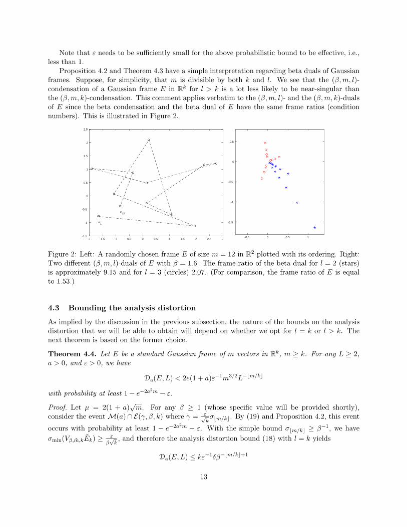
Proposition 4.2 and Theorem 4.3 have a simple interpretation regarding beta duals of Gaussianframes. Suppose, for simplicity, that m is divisible by both k and l. We see that the (β,m, l)-condensation of a Gaussian frame E in Rk for l > k is a lot less likely to be near-singular thanthe (β,m, k)-condensation. This comment applies verbatim to the (β,m, l)- and the (β,m, k)-dualsof E since the beta condensation and the beta dual of E have the same frame ratios (conditionnumbers). This is illustrated in Figure 2.

-2 -1.5 -1 -0.5 0 0.5 1 1.5 2 2.5 3-1.5

-1

-0.5

0

0.5

1

1.5

2

2.5

e1

e12

-0.5 0 0.5 1

-1.5

-1

-0.5

0

0.5

Figure 2: Left: A randomly chosen frame E of size m = 12 in R2 plotted with its ordering. Right:Two different (β,m, l)-duals of E with β = 1.6. The frame ratio of the beta dual for l = 2 (stars)is approximately 9.15 and for l = 3 (circles) 2.07. (For comparison, the frame ratio of E is equalto 1.53.)

4.3 Bounding the analysis distortion

As implied by the discussion in the previous subsection, the nature of the bounds on the analysisdistortion that we will be able to obtain will depend on whether we opt for l = k or l > k. Thenext theorem is based on the former choice.

Theorem 4.4. Let E be a standard Gaussian frame of m vectors in Rk, m ≥ k. For any L ≥ 2,a > 0, and ε > 0, we have

Da(E,L) < 2e(1 + a)ε−1m3/2L−bm/kc

with probability at least 1− e−2a2m − ε.

Proof. Let µ = 2(1 + a)√m. For any β ≥ 1 (whose specific value will be provided shortly),

consider the event M(a) ∩ E(γ, β, k) where γ = ε√kσbm/kc. By (19) and Proposition 4.2, this event

occurs with probability at least 1 − e−2a2m − ε. With the simple bound σbm/kc ≥ β−1, we have

σmin(Vβ,m,kEk) ≥ εβ√k, and therefore the analysis distortion bound (18) with l = k yields

Da(E,L) ≤ kε−1δβ−bm/kc+1

13

for any δ > 0 such that (β, δ) ∈ Sµ,L. Now we specify the pair (β, δ) ∈ Sµ,L. With α = bm/kc − 1,we set β = L(α+ 1)/(α+ 2) and δ = µ(α+ 2)/L as in Lemma 3.2 and obtain

Da(E,L) < kε−1µebm/kcL−bm/kc.

Substituting the value of µ and simplifying completes the proof.

The parameter a is largely inconsequential and could be fixed, e.g. a = 1. Meanwhile, themost favorable choice of ε depends on the probabilistic assurance as well as the analysis distortionguarantee that is desired. For example, if k is comparable to logL, then choosing ε = L−ηbm/kc

for some (small) η > 0 would guarantee, without affecting the analysis distortion significantly, thatthe failure probability is exponentially small in m. However, when k is large (or L is small), thischoice will not correspond to a practical scenario. In any case, the above theorem is sufficient toconclude that as m→∞, we have Da(E,L) = O

(L−(1+o(1))m/k

)with probability 1− o(1).

We now present an alternative probabilistic bound on the analysis distortion based on the choicel > k, which will ultimately lead to the proof of Theorem 1.1.

Theorem 4.5. Let E be a standard Gaussian frame of m vectors in Rk, m > k. For any L ≥ 2,a > 0, ε > 0, and l such that k < l ≤ m, we have

Da(E,L) < 4e(1 + a)ε−1m3/2l−1L−bm/lc (21)

with probability at least 1− e−2a2m − 2(10 + 8√

log ε−1)kel/2εl−k+1.

Proof. We follow the same route as in Theorem 4.4. Again, let µ := 2(1 + a)√m, and for β ≥ 1

to be specified shortly, consider the event M(a) ∩ E(γ, β, l) (recall the definition given in (20))where γ = εσbm/lc

√l/2. By (19) and Theorem 4.3, this event occurs with probability at least

1−e−2a2m−2(10+8√

log ε−1)kel/2εl−k+1. Again using σbm/lc ≥ β−1, we have σmin(Vβ,m,lEl) ≥ ε√l

2β ,and therefore the analysis distortion bound (18) yields

Da(E,L) ≤ 2ε−1δβ−bm/lc+1

for any δ > 0 such that (β, δ) ∈ Sµ,L. With α = bm/lc − 1, we again set β = L(α+ 1)/(α+ 2) andδ = µ(α+ 2)/L as in Lemma 3.2 and obtain

Da(E,L) < 2ε−1µebm/lcL−bm/lc.

Substituting the value of µ and simplifying completes the proof.

When l > k and ε is small, Theorem 4.5 provides a more favorable bound on the failure prob-ability compared to Theorem 4.4 because of the presence of εl−k+1. We now turn this observationinto a concrete form by suitably choosing the values of ε and l.

For simplicity, let a = 1. For any (small) θ ∈ (0, 1), let ε = L−θm/k and l = k + bθkc. Supposek ≥ 1/θ and m/k ≥ (1 + θ)/θ2. Clearly we have l > k and also⌊m

l

⌋≥⌊

m

(1 + θ)k

⌋≥ m

(1 + θ)k− 1 ≥ (1− θ)m

k

so that the error bound (21) is effective and can be simplified to

Da(E,L) < 8em3/2k−1L−(1−2θ)mk .

14

Furthermore, this bound is simultaneously valid for all L ≥ 2 if the event M(1) ∩ Eθ where

Eθ :=∞⋂L=2

E(γ, β, l)

occurs. Here γ = εσbm/lc√l/2 and β = L(α+ 1)/(α+ 2) with α = bm/lc − 1 are as in the proof of

Theorem 4.5.By Theorem 4.3, the probability of E(γ, β, l)c is bounded by 2(10 + 8

√log ε−1)kel/2εl−k+1. To

simplify this bound, note that 13√

log 2 > 10 so that 10 + 8√

log ε−1 < 21√

(m/k) logL. Hence,together with the observation that l − k + 1 = bθkc+ 1 > θk, we have

P(E(γ, β, l)c) ≤ 2 exp

k

(log 21 +

1

2log

m

k+

1

2log logL+

1

2(1 + θ)

)−mθ2 logL

.

There exists an absolute constant c1 > 0 such that if mk ≥

c1θ2

log mk , then

k

(log 21 +

1

2log

m

k+

1

2log logL+

1

2(1 + θ)

)≤ 1

2mθ2 logL

so thatP(E(γ, β, l)c) ≤ 2L−

12θ2m.

By readjusting the value of c1 if necessary, we are guaranteed that m ≥ 4/θ2 so that 12θ

2m ≥ 2 and

P(Ecθ) ≤∞∑L=2

2L−12θ2m < 2

(2−

12θ2m +

∫ ∞2

t−12θ2m dt

)≤ 6 · 2−

12θ2m.

Setting η = 2θ and restricting θ ∈ (0, 1/2), we obtain the following corollary:

Corollary 4.6. There exists an absolute constant c1 > 0 such that if η ∈ (0, 1), and m and k aresuch that k ≥ 2/η and m

k ≥c1η2

log mk , a standard Gaussian frame E of m vectors in Rk satisfies

Da(E,L) < 8em3/2k−1L−(1−η)m/k

for all L ≥ 2 with probability at least 1− 6 · 2−18η2m − e−2m.

Proof of Theorem 1.1. We make the following observations. First, increasing the value of c1in Corollary 4.6 if necessary, the assumption m

k ≥c1η2

log mk implies that m

k ≥c1η2

, and therefore

8e(mk

)3/2< e4+1.5 log(m/k) < Lc3η

2m/k,

where c3 = 8/c1. Again increasing the value of c1 if necessary, we can assume that c3 ≤ 1 sothat 1 − η − c3η2 ≥ 1 − 2η. Next, we can restrict η ∈ (0, 1/2), set η′ = 2η and c′1 = 4c1. Thisyields the error bound

√kL−(1−η

′)m/k. For the probability guarantee, note that m = k(m/k) ≥(4/η′)(c′1/η

′2) = 4c′1/η′3. Once again increasing the value of c′1 if necessary, we can find an absolute

constant c2 > 0 such that 6 · 2−132η′2m + e−2m ≤ e−c2η

′2m for all admissible m, hence Theorem 1.1follows once we denote η′ by η and c′1 by c1 again.

15

4.4 Results for sub-Gaussian distributions

Our methods are applicable in the case of any other probability distribution governing the frameE since the basic quantization algorithm and the resulting bound on the analysis distortion aredeterministic. As we discussed in depth for the Gaussian distribution, two types of probabilisticbounds need to be established for E: The first is an upper bound on ‖E‖2→∞ which may bereplaced by an upper bound on σmax(E), and the second is a lower bound on σmin(Vβ,m,lEl).

For simplicity we will continue to assume that the entries of E are chosen independently, butnow more generally from a centered sub-Gaussian distribution of unit variance. Recall that arandom variable X on R is called sub-Gaussian if there exists K > 0, called the sub-Gaussianmoment of X, such that P(|X| > t) ≤ 2e−t

2/K2for all t > 0 [30].

Regarding the upper bound on σmax(E), the generalization of Proposition 4.1 to sub-Gaussianrandom matrices says that

P(σmax(E) > K1(

√m+

√k) + t

)≤ 2e−t

2/K22

for positive absolute numerical constants K1 and K2 (see, e.g. [28]). Consequently, we may simplyset µ := 2(K1 + 1)

√m which is essentially the same as in the Gaussian case, albeit for a slightly

larger constant. In the special case of bounded distributions, then it is actually possible to setµ := O(

√k) which is even better than the Gaussian case, and in a certain sense, the best we can

ever achieve.As for the lower bound on σmin(Vβ,m,lEl), note that the entries of Ω := Vβ,m,lEl are also

independent because each entry of E influences at most one entry of Vβ,m,lEl, thanks to the structureof the beta condensation matrix Vβ,m,l. (Again thanks to this structure, one may even weaken theentry-wise independence assumption we made above.) In addition, the entries of Ω are identicallydistributed and are centered sub-Gaussian random variables [30, Lemma 5.9]. Proposition 4.2and Theorem 4.3 have also been generalized to the sub-Gaussian case, and in fact as part of onecommon result: If Ω is an l × k matrix whose entries are independent and identically distributedsub-Gaussian random variables with zero mean and unit variance, then

P(σmin(Ω) ≤ ε

(√l −√k − 1

))≤ (K3ε)

l−k+1 + cl (22)

where K3 > 0 and c ∈ (0, 1) depend only on the sub-Gaussian moment of the entries [27].With these tools, it is possible to obtain fairly strong bounds on the analysis distortion of

sub-Gaussian frames, but not quite as strong as those obtainable for the Gaussian case. Themain problem stems from the presence of the cl term in (22) which, as explained in [27, 28],is characteristic of the sub-Gaussian case. As such, this term prevents us from stating an exactanalog of Theorem 1.1. In particular, l must be required to go to infinity in order to ensure that thefailure probability bound vanishes as m→∞. Consequently, the resulting analysis distortion boundwould not be near-optimal in the sense we currently have, but of the form L−o(m). For example, ifwe let l ≈ mκk1−κ for some κ ∈ (0, 1), then we can obtain a “root-exponential” distortion boundof the form L−(m/k)

1−κwhich is guaranteed also up to root-exponentially small failure probability.

Alternatively, the more conservative choice l ≈ k + logm would result in a distortion bound of theform L−m/(k+logm) up to a failure probability of O(m−a) where c = e−a.

16

Acknowledgements

The authors would like thank Thao Nguyen, Rayan Saab and Ozgur Yılmaz for the useful conver-sations on the topic of this paper and the anonymous referees for the valuable comments and thereferences they have brought to our attention.

A Appendix

Lemma A.1. Let ξ ∼ N (0, Il). For any 0 < ε ≤ 1, we have

P(‖ξ‖2 ≤ ε

√l)≤ εle(1−ε2)l/2.

Proof. For any t ≥ 0, we have

P(‖ξ‖22 ≤ ε2l

)≤∫Rle(ε

2l−‖x‖22)t/2 e−‖x‖22/2

(2π)l/2dx = eε

2tl/2

∫Rl

e−(1+t)‖x‖22/2

(2π)l/2dx =

(eε

2t

1 + t

)l/2.

Choosing t = ε−2 − 1 yields the desired bound.

Proof of Theorem 4.3. For an arbitrary τ > 1, let E1 be the event ‖Ω‖2→2 ≤ 2τ√l. Propo-

sition 4.1 with m = l, E = Ω, t = 2(τ − 1)√l implies

P(Ec1) ≤ e−2(τ−1)2l.

Next, consider a ρ-net Q of the unit sphere of Rk with |Q| ≤ 2k(1 + 2/ρ)k−1 (see [27, Proposition2.1]), where we set ρ = ε/(4τ). Let E2 be the event ‖Ωz‖2 ≥ ε

√l, ∀z ∈ Q. For each fixed z ∈ Rk

with unit norm, Ωz has entries that are i.i.d. N (0, 1). By Lemma A.1, we have

P(Ec2) ≤ |Q|εle(1−ε2)l/2 ≤ 2k(ε+ 8τ)k−1εl−k+1e(1−ε2)l/2.

Suppose the event E1 ∩ E2 occurs. For any unit norm x ∈ Rk, there exists a z ∈ Q such that‖x− z‖2 ≤ ρ. Then ‖Ω(x− z)‖2 ≤ 2τρ

√l = ε

√l/2 and ‖Ωz‖2 ≥ ε

√l, so that

‖Ωx‖2 ≥ ‖Ωz‖2 − ‖Ω(x− z)‖2 ≥ ε√l/2,

hence σmin(Ω) ≥ ε√l/2. It follows that F :=

σmin(Ω) ≤ ε

√l/2⊂ Ec1 ∪ Ec2, and therefore

P (F) ≤ e−2(τ−1)2l + 2k(ε+ 8τ)k−1εl−k+1el/2.

We still have the freedom to choose τ > 1 as a function of ε, l, and k. For simplicity, we chooseτ = 1 +

√log ε−1 so that e−2(τ−1)

2l = ε2l. Noting that 1 + k(1 + 8τ)k−1 < (2 + 8τ)k, we obtain

P (F) < εl−k+1(

1 + 2k(1 + 8τ)k−1el/2)< 2

(10 + 8

√log ε−1

)kel/2εl−k+1.

17

References

[1] R.G. Baraniuk, S. Foucart, D. Needell, Y. Plan, and M. Wootters. Exponential decay ofreconstruction error from binary measurements of sparse signals. CoRR, abs/1407.8246, 2014.

[2] J.J. Benedetto, A.M. Powell, and O. Yılmaz. Second-order sigma-delta (Σ∆) quantization offinite frame expansions. Appl. Comput. Harmon. Anal., 20(1):126–148, 2006.

[3] J.J. Benedetto, A.M. Powell, and O. Yılmaz. Sigma-delta quantization and finite frames.Information Theory, IEEE Transactions on, 52(5):1990–2005, 2006.

[4] J. Blum, M. Lammers, A.M. Powell, and O. Yılmaz. Sobolev duals in frame theory andsigma-delta quantization. Journal of Fourier Analysis and Applications, 16(3):365–381, 2010.

[5] B.G. Bodmann and V.I. Paulsen. Frame paths and error bounds for sigma-delta quantization.Appl. Comput. Harmon. Anal., 22(2):176–197, 2007.

[6] B. Chazelle. The discrepancy method: randomness and complexity. Cambridge UniversityPress, 2002.

[7] K. Dajani and C. Kraaikamp. Ergodic theory of numbers, volume 29 of Carus MathematicalMonographs. Mathematical Association of America, Washington, DC, 2002.

[8] I. Daubechies, R.A. DeVore, C.S. Gunturk, and V.A. Vaishampayan. A/D conversion withimperfect quantizers. IEEE Trans. Inform. Theory, 52(3):874–885, 2006.

[9] K.R. Davidson and S.J. Szarek. Local operator theory, random matrices and Banach spaces. InHandbook of the geometry of Banach spaces, Vol. I, pages 317–366. North-Holland, Amsterdam,2001.

[10] K.R. Davidson and S.J. Szarek. Addenda and corrigenda to: “Local operator theory, randommatrices and Banach spaces”. In Handbook of the geometry of Banach spaces, Vol. 2, pages1819–1820. North-Holland, Amsterdam, 2003.

[11] P. Deift, F. Krahmer, and C.S. Gunturk. An optimal family of exponentially accurate one-bit sigma-delta quantization schemes. Communications on Pure and Applied Mathematics,64(7):883–919, 2011.

[12] M.S. Derpich, E.I. Silva, D.E. Quevedo, and G.C. Goodwin. On optimal perfect reconstructionfeedback quantizers. IEEE Trans. Signal Process., 56(8, part 2):3871–3890, 2008.

[13] A. Edelman. Eigenvalues and condition numbers of random matrices. SIAM Journal on MatrixAnalysis and Applications, 9(4):543–560, 1988.

[14] I. Galton and H.T. Jensen. Oversampling parallel delta-sigma modulator A/D conversion. Cir-cuits and Systems II: Analog and Digital Signal Processing, IEEE Transactions on, 43(12):801–810, Dec 1996.

[15] V.K. Goyal, M. Vetterli, and N.T. Thao. Quantized overcomplete expansions in RN : analysis,synthesis, and algorithms. Information Theory, IEEE Transactions on, 44(1):16–31, 1998.

18

[16] C. S. Gunturk, M. Lammers, A. M. Powell, R. Saab, and O. Yılmaz. Sobolev duals for randomframes and Σ∆ quantization of compressed sensing measurements. Found. Comput. Math.,13(1):1–36, 2013.

[17] C.S. Gunturk. One-bit sigma-delta quantization with exponential accuracy. Communicationson Pure and Applied Mathematics, 56(11):1608–1630, 2003.

[18] C.S. Gunturk. Mathematics of analog-to-digital conversion. Comm. Pure Appl. Math.,65(12):1671–1696, 2012.

[19] M. Iwen and R. Saab. Near-optimal encoding for sigma-delta quantization of finite frameexpansions. Journal of Fourier Analysis and Applications, 19(6):1255–1273, 2013.

[20] F. Krahmer, R. Saab, and O. Yılmaz. Sigma-delta quantization of sub-gaussian frame ex-pansions and its application to compressed sensing. Information and Inference, 3(1):40–58,2014.

[21] M. Lammers, A.M. Powell, and O. Yılmaz. Alternative dual frames for digital-to-analogconversion in sigma-delta quantization. Adv. Comput. Math., 32(1):73–102, 2010.

[22] M.C. Lammers, A.M. Powell, and O. Yılmaz. On quantization of finite frame expansions:sigma-delta schemes of arbitrary order. Proc. SPIE 6701, Wavelets XII, 670108, 6701:670108–670108–9, 2007.

[23] J. Matousek. Geometric discrepancy, volume 18 of Algorithms and Combinatorics. Springer-Verlag, Berlin, 1999. An illustrated guide.

[24] V. Molino. Approximation by Quantized Sums. PhD thesis, New York University, 2012.

[25] W. Parry. On the β-expansions of real numbers. Acta Math. Acad. Sci. Hungar., 11:401–416,1960.

[26] A.M. Powell, R. Saab, and O. Yılmaz. Quantization and finite frames. In Finite Frames, pages267–302. Springer, 2013.

[27] M. Rudelson and R. Vershynin. Smallest singular value of a random rectangular matrix.Communications on Pure and Applied Mathematics, 62(12):1707–1739, 2009.

[28] M. Rudelson and R. Vershynin. Non-asymptotic theory of random matrices: extreme singularvalues. In Proceedings of the International Congress of Mathematicians. Volume III, pages1576–1602. Hindustan Book Agency, New Delhi, 2010.

[29] N.T. Thao and M. Vetterli. Lower bound on the mean-squared error in oversampled quan-tization of periodic signals using vector quantization analysis. Information Theory, IEEETransactions on, 42(2):469–479, 1996.

[30] R. Vershynin. Introduction to the non-asymptotic analysis of random matrices. In Compressedsensing, pages 210–268. Cambridge Univ. Press, Cambridge, 2012.

19