Coupling of WRF with the EPA’s Community Multiscale Air Quality (CMAQ) Model

Prof. Daewon Byun (PI)C.K. Song & P. Percell

University of HoustonInstitute for Multidimensional Air Quality Studies

Collaborators:Ken. Schere (PO) & Jon Pleim, NOAA/ARL & EPA/ORD ASMD

Paula Davidson, Jeff McQueen, NOAA/NCEPand many others…

build a linkage between the meteorological and air quality model while maintaining the dynamic description of the base model as closely as possible

Use meteorological data (state variable definitions) that minimize errors during the temporal interpolations in air quality model.

Goal: Build Dynamically Consistent Coupled WRF/nmm & CMAQ Air Quality Forecasting System

Development objectives

1) One-way coupling:Loose coupling (NOAA & EPA RTP group)Tight coupling (University of Houston & EPA)

2) Provide algorithms for the coupling

3) Verification of coupling

Numerical Weather Prediction (NWP)

~ 1950s with the advent of modern computer

Simplified Dynamics Models

barotropic models

baroclinic models

hydrostatic models

incompressible atm. assumption.

compressible atm. assumption

pseudo nonhydrostatic model

Fully-compressible atm. models

Air Quality Models (AQMs)

~ 1970s started by chemical engineers

Simulates pollutant transport only.

Meteorological data as external inputs

Objective analyzed winds

•UAM & ROM utilize Implicit/Explicit assumption of

hydrostatic & incompressible atmosphere

NWP output

•RADM (late 1980s) is the first (?) model linked with an NWP model (e.g., MM4)

•SAQM – linked with MM5 (pseudo nonhydrostatic)

•CMAQ - fully compressible & generalized coordinate formulation (linked with MM4, MM5, RAMS, CALMET, WRF/EM, WRF/EH, etc…)

Brief History of Atmospheric Models

(USA only…)

Brief Introduction of CMAQ

•“First principles” description of atmospheric systemConservation laws – mass, energy, momentum, …

•Multiple scale atmospheric dynamicsMeso-gamma, urban, regional, global scalesDaily, episodic, seasonal, annual time scales

•Multiple atmospheric pollutantsOzone, acid deposition, eutrophicationFine particles, visibilityTracer transportToxics

Science Characteristics of EPA’s Community Multiscale Air Quality Model (CMAQ)

References; Byun & Ching (1999), Byun & Schere (2005) & papers by many others….

Degree of Comprehensiveness in science process representation

Aerosol thermodynamics codes: equilibrium model, hybrid model, dynamic model

Aerosol distribution: modal & sectionalAdvection: finite volume methods (Botts, PPM, YAM, etc..)Diffusion: K-theory & Asymmtric Convective Model (Pleim & Chang)Deposition: RADM-scheme (Weseley et al, 1989), M3DRY (Pleim)Gas-phase: CB-4, RADM, SAPRC99, Air Toxics, Hg, etc…

Degree of Generality in the governing equations

Example for the atmospheric dynamics and thermodynamics: fully compressible nonhydrostatic formulation vs. hydrostatic, nondivergent flow assumption

Note: More general and comprehensive formulations do not necessarily increase numerical complexity

Generalized coordinate system expands model application domain with minimal increase in the computational cost

Communty Multiscale Air Quality (CMAQ) System

SMOKE

Meteorologicalmodels

Emissionsmodels

Analysis&

Visualization

Chemistry

Clouds Aerosols

DiffusionAdvection

Chemistry - Transport model

USERS

EnvironmetalData

EnvironmentalData

ScienceFindings

Policy Related Information

Interface Processors

Plume-in-Grid

MM5

WRF/EM

WRF/NMM

EPS2

WRF/nmm

WRF/nmmPostprocessors

(vertical/horizontal)

PREMAQ (modified)

CMAQ

Loose coupling Tight coupling

WRF/nmm

Interface Processor

CMAQ/nmm

Components of Coupled system

Developed by EPA

Under development by UofH

Spatial interpolation

Lambert conformal projection On rotated lat/long coordinate?

Under development by UofH

Consistent governing set of equations & state variables

Consistent coordinates and grid structures

Consistent numerics & physics, and parameterizations

Consistent use of basic input data (e.g., Land Use/Land Cover, topography)

Flexibility: ability to help diverse stake holders (research – regulatory application)

What are the main science issues of the NWP & AQM coupling?

WRF (EM core)

Governing Eq. Formulation : Flux formPrognostic variable :

Momentum, Dry entropy, Geopotential, Column massHorizontal grid : Arakawa C grid (Lambert Conformal)Vertical coordinate : Terrain following sigma

WRF (NMM core)

Governing Eq. Formulation : Advective formPrognostic variable :

Velocity, Temperature, Pressure, Column massHorizontal grid : Arakawa E grid (Rotated Lat./Lon.)Vertical coordinate : Hybrid(Terrain following sigma/Pressure)

zszs

zzs

szs Jf

svJ

mJm

tJ VτVVVV ρ

∂∂ρρ

∂ρ∂

×++•∇+ 33

2 ˆˆ)()(

ssss

ss Jsp

zs

gmJpmJ Fρ

∂∂

∂∂

ρρρ =⎥

⎦

⎤⎢⎣

⎡Φ∇⎟

⎠⎞

⎜⎝⎛−∇+

∂ ( ρJ sw )∂ t

+ m 2 ∇ s •ρJ sw V z

m⎛ ⎝ ⎜ ⎞

⎠ ⎟ +

∂ ( ρJ sw ˆ v 3 )∂ s

+ ρJ smρ

∂ p∂ s

+∂ Φ∂ s

⎛

⎝ ⎜

⎞

⎠ ⎟

∂s∂ z

⎛ ⎝ ⎜ ⎞

⎠ ⎟ = ρ Js F3 +

wQ ρ

ρ⎛

⎝ ⎜

⎞

⎠ ⎟

∂ (ρJs )∂t

+ m2∇s •ρJs

ˆ V sm2

⎛

⎝ ⎜

⎞

⎠ ⎟ +

∂ (ρJs ˆ v 3 )∂s

= JsQρ ζ∂σ∂σ

∂σ∂ QJ

svJ

mJm

tJ

ssss

ss =+⎟⎟

⎠

⎞⎜⎜⎝

⎛•∇+

)ˆ(ˆ)( 3

22 V

∂ (ϕi Js )∂t

+ m2∇ s •ϕ i Js

ˆ V sm2

⎛

⎝ ⎜

⎞

⎠ ⎟ +

∂(ϕ i Js ˆ v 3 )∂s

= JsQϕ i)ln()ln(

ood

oovd R

TTC

ρρρρσ −=

γ

⎟⎟⎠

⎞⎜⎜⎝

⎛ Θ=

o

do p

Rpp

Fully Compressible Atmosphere (OOyama, 1990) used for CMAQ

Horizontal grid : Arakawa C grid (Lambert Conformal)

Map Factor & Grid Resolution

m = n = 1LATGRD3=1For WRF/NMM[Rotated Lat./Lon.]

LATGRD3=2For WRF/EM (WCIP)[Lambert Conformal]

LATGRD3=2For MM5 (MCIP)[Lambert Conformal]

NoteMap Scale (m)ID in Models-3 IOAPI

1

1

2

1

2

1

1

)4/tan()4/tan(ln

)2/sin()2/sin(ln

)4/tan()4/tan(

)2/sin()2/sin(

−

⎥⎦

⎤⎢⎣

⎡⎟⎟⎠

⎞⎜⎜⎝

⎛−−

⎥⎦

⎤⎢⎣

⎡−−

=

⎥⎦

⎤⎢⎣

⎡−−

−−

=

φπφπ

φπφπ

φπφπ

φπφπ

n

mn

1

1

2

1

2

1

1

)4/tan()4/tan(ln

)2/sin()2/sin(ln

)4/tan()4/tan(

)2/sin()2/sin(

−

⎥⎦

⎤⎢⎣

⎡⎟⎟⎠

⎞⎜⎜⎝

⎛−−

⎥⎦

⎤⎢⎣

⎡−−

=

⎥⎦

⎤⎢⎣

⎡−−

−−

=

φπφπ

φπφπ

φπφπ

φπφπ

n

mn

dydxxx centcent

== ),()ˆ,ˆ( 00

21 φλ

dydxxx centcent

== ),()ˆ,ˆ( 00

21 φλ

.),.(

).,.()ˆ,ˆ( 21

constdyLatfdx

LatLonxx

rotated

rotatedrotated

==

=

Generalized Vertical Coordinate Forms

For WRF/NMM

For WRF/EM (WCIP)

For MM5 (MCIP)

Vertical Jacobian, JsVertical Coordinate, s

)()(

Ts

Tpo pp

pp−−

=σgppJ T

s ρ)( −

=pos σ−= 1

η−= 1s)()(

Ts

T

ππππη

−−

=g

J s ρµ

= Ts ππµ −=

),,(~)()(),,,(~* tyxpBpAtyxp T ηηη += *

~)()(~~pBpAJgp

T ηη

ηηρ

η η ∂∂

+∂

∂=−=

∂∂

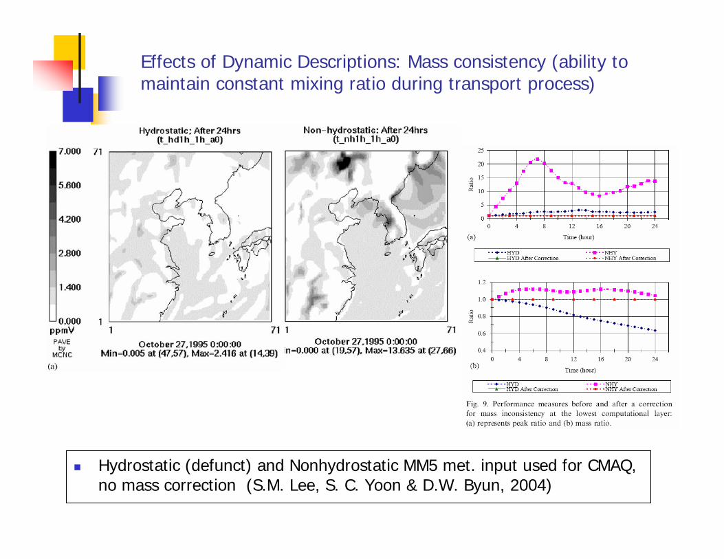
Effects of Dynamic Descriptions: Mass consistency (ability to maintain constant mixing ratio during transport process)

Hydrostatic (defunct) and Nonhydrostatic MM5 met. input used for CMAQ, no mass correction (S.M. Lee, S. C. Yoon & D.W. Byun, 2004)

µππη t−

= ts ππµ −= gJ s ρµ /=

iqssissi

ssi QJ

svJq

mJqm

tJq

=+⎟⎠⎞

⎜⎝⎛•∇+

∂ρ∂ρ

∂ρ∂ )ˆ(ˆ)( 3

22 v

How to link dynamics between WRF & CMAQ?

CMAQ

WRF EM coordinate information

WRF EM dynamic variables

1vU µ= 2vV µ= wW µ= 3vµ=Ω

On-line model: All the state variables available at integration time step

Off-line model: What temporal averaging schemes should be used?

ˆs sJρ< >v sJρ< >

sJρ ˆs sJρ vˆ sv sJρ ˆs sJρ vˆ sv

ˆ s< >v

CMAQ

WRF/EM

Possibilities

ˆ s< >v

zmgmJ

mJ

vvv ˆˆˆ 22

µρρη

ηξ

ξ ==gmm

J22

Ω−=ξ

ρ ξ &

⎩⎨⎧

=−=

==)at top 0 bottom,at 1sfor (1)at top 1 bottom,at 0sfor (

ˆ 3

ss

x ξ

)ˆ()(ˆ2 zs

mhH

mJ

vv ρρ

ξξ −

=

⎟⎠⎞

⎜⎝⎛+∇•−+=

zwhm

tv

∂∂ς

∂∂ς

ςς )ˆ(ˆ3 v32

32

ˆ)(ˆ vm

hHv

mJ s−

=ρρ ς

For WRF/EM Core, consider how to apply temporal averaging for all the components in the conservation eq.

Cf: for EH Dynamic Core – vertical coordinate “fixed” (NCAR dropped EH)

Previous Study: Use of instantaneous WRF output

•Instantaneous Mass-Jacobian for coordinate •Instantaneous Mass-Jacobian weighted Contravariant wind

Instantaneous Vertical Velocity at layer 1

MM5 WRF mass

(31,50)(31,50)2000/08/26 20UTC (14LST)

Vertical velocity multiplied with Jacobian-weighted density (instantaneous)

MM5 WRF mass WRF height

2000/08/26/06UTC

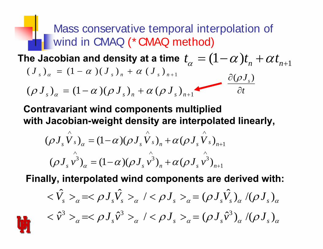
Mass conservative temporal interpolation of wind in CMAQ (*CMAQ method)

1(1 ) n nt t tα α α += − +

1( ) (1 )( ) ( )s s n s nJ J Jαρ α ρ α ρ += − +

1( ) (1 ) ( ) ( )s s n s nJ J Jα α α += − +The Jacobian and density at a time

1( ) (1 )( ) ( )s s ss s n s nJ V J V J Vαρ α ρ α ρ∧ ∧ ∧

+= − +

Contravariant wind components multiplied with Jacobian-weight density are interpolated linearly,

3 3 31( ) (1 )( ) ( )s s n s nJ v J v J vαρ α ρ α ρ

∧ ∧ ∧

+= − +

( )sJt

ρ∂∂

ˆ ˆ ˆ/ ( ) /( )s s s s s s sV J V J J V Jα α α α αρ ρ ρ ρ< > =< > < > =

Finally, interpolated wind components are derived with:

3 3 3ˆ ˆ ˆ/ ( ) /( )s s s sv J v J J v Jα α α α αρ ρ ρ ρ< > =< > < > =

Test of other temporal interpolation methods

Method 1 (both averaged coordinate and wind components)

Method1.5 (instantaneous µ and averaged wind component)

Method 2 (use interpolated wind but no density interpolation)

ˆ( )ˆ( )

s ss

s

J VV

Jα

αα

ρρ

< > =

ˆ( )ˆ( )

s ss

s

J VV

Jα

αα

ρρ

< > =3

3 ˆ( )ˆ( )

s

s

J vv

Jα

αα

ρρ

< > =

ˆ ˆ( )s sV Vα α< > = 3 3ˆ ˆ( )v vα α< > =

33 ˆ( )ˆ

( )s

s

J vv

Jα

αα

ρρ

< > =

Note: Current tests use instantaneous Mass*Jacobian as the verticalcoordinate in CMAQ

sJ gρ µ=

1 day simulation with 1hrly met. data from WRF/EM-CMAQ coupling

1. Except CMAQ method, mass is decreasing with time for other methods. No strong diurnal variation

2. CMAQ> M1.5: the variation of coordinate variables in 24 hrs is larger than that in 1hr. Thus, in linkage methods which use averaged values, it is also needed to consider time-averaged coordinate variables for building model coordinate.

3. to maintain mass conservation, there is no need to feed met data at the

TIME (UTC)

0 5 10 15 20

Standard Deviation (ppm

V) 0.000.200.400.600.801.001.201.401.601.802.002.202.40

0

Mean (ppm

V)

0.8600.8800.9000.9200.9400.9600.9801.0001.020

CMAQ method Method 2

Method 1

Method1.5

NWP models can conserve air mass well! ~ 0.05 %/hr

Diurnal behavior of error growth (without correction)

CMAQ interpolationmethod

Method1.5

Daytime

In other methods, error growth is too fast!

Error growth in the CMAQ method is due to the convective cells from NWP

Nighttime

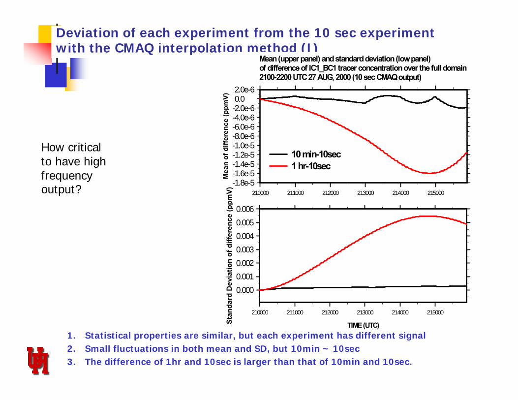
Deviation of each experiment from the 10 sec experiment with the CMAQ interpolation method (I)

TIME (UTC)

210000 211000 212000 213000 214000 215000

Stan

dard

Dev

iatio

n of

diff

eren

ce (p

pmV)

0.0000.0010.0020.0030.0040.0050.006

Mean (upper panel) and standard deviation (low panel)of difference of IC1_BC1 tracer concentration over the full domain2100-2200 UTC 27 AUG, 2000 (10 sec CMAQ output)

210000 211000 212000 213000 214000 215000

Mea

n of

diff

eren

ce (p

pmV)

-1.8e-5-1.6e-5-1.4e-5-1.2e-5-1.0e-5-8.0e-6-6.0e-6-4.0e-6-2.0e-60.02.0e-6

10 min-10sec1 hr-10sec

1. Statistical properties are similar, but each experiment has different signal2. Small fluctuations in both mean and SD, but 10min ~ 10sec3. The difference of 1hr and 10sec is larger than that of 10min and 10sec.

How critical to have high frequency output?

Layer mean(shaded) and standard deviation (white line)of difference of IC1_BC1 tracer concentrationbetween 10min experiment and 10sec experiment

TIME (HHMM)

2100

2105

2110

2115

2120

2125

2130

2135

2140

2145

2150

2155

VER

TIC

AL L

AYER

123456789

10111213141516171819202122232425262728293031323334353637383940414243

Layer mean(shaded) and standard deviation (white line)of difference of IC1_BC1 tracer concentrationbetween 1hr experiment and 10sec experiment

TIME (HHMM)

2100

2105

2110

2115

2120

2125

2130

2135

2140

2145

2150

2155

VER

TIC

AL L

AYER

123456789

10111213141516171819202122232425262728293031323334353637383940414243

-0.00180 -0.00150 -0.00120 -0.00090 -0.00060 -0.00030 0.00000 0.00030

0.00030.0003 0.00030.0003

0.0003

0.0003

0.00060.0006 0.0009

0.00090.0009

0.0009

0.0009

0.00120.0012

0.00150.0015

0.00210.0018 0.0018

0.0012

0.0012

0.00120.0012

0.0012

0.0009

0.0003

0.0006

0.0006

0.00060.0003

0.0003

0.0003

Deviation of each experiment from the 10 sec experiment with the CMAQ interpolation method (II)

10min – 10sec 1hr – 10sec

1. Layer mean difference in time-vertical cross-section2. Large difference near surface due to surface forcing3. Same message (The difference of 1hr and 10sec is larger than that of 10min and

10sec)

Deviation of each experiment from the 10 sec output experiment with the CMAQ interpolation method (III):Layer 1 at 21:45 UTC, August 27, 2000

1. In this case, the dynamical variation in less 10min are not well represented in the WRF simulation Related with Dr. Bill Skaramock’s KE spectra analysis result

2. Possible to use a larger time step than meteorological integration time step without losing mass consistency of wind fields.

We have revealed that the wind from the WRF mass core is very mass-consistent most of the timeEven without mass adjustment, the off-line WRF-CMAQ system has conserved the mass of pollutants well by using the mass conservative temporal interpolation of wind in CMAQ except for the convective cells.Higher met. data transfer frequency makes the off-line CMAQ model results closer to the on-line model.Also, this study clearly indicates that the mass-consistency of wind fields can be maintained with an output time step larger than met. time step because the WRF mass provides the mass-consistent wind field.

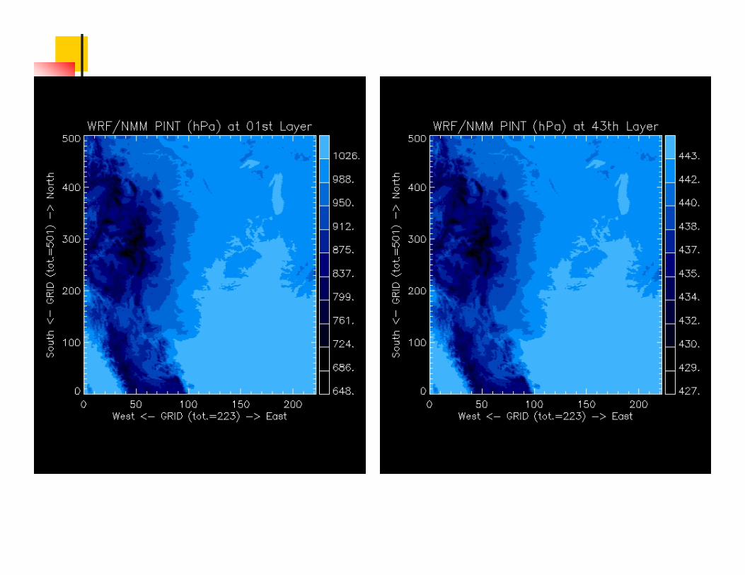
Vertical grid system of WRF/nmm

Terrain-following hybrid pressure-sigma coordinate (Arakawa and Lamb, 1977)

Lorenz vertical staggering- Geopotential and nonhydrastaticpressure are on the interfaces

- 3-D velocity components and temperature are on the middle layers

From Janjic (2003)

Consistent coordinates and grid structures

sigma values for each levels of WRF/NMM

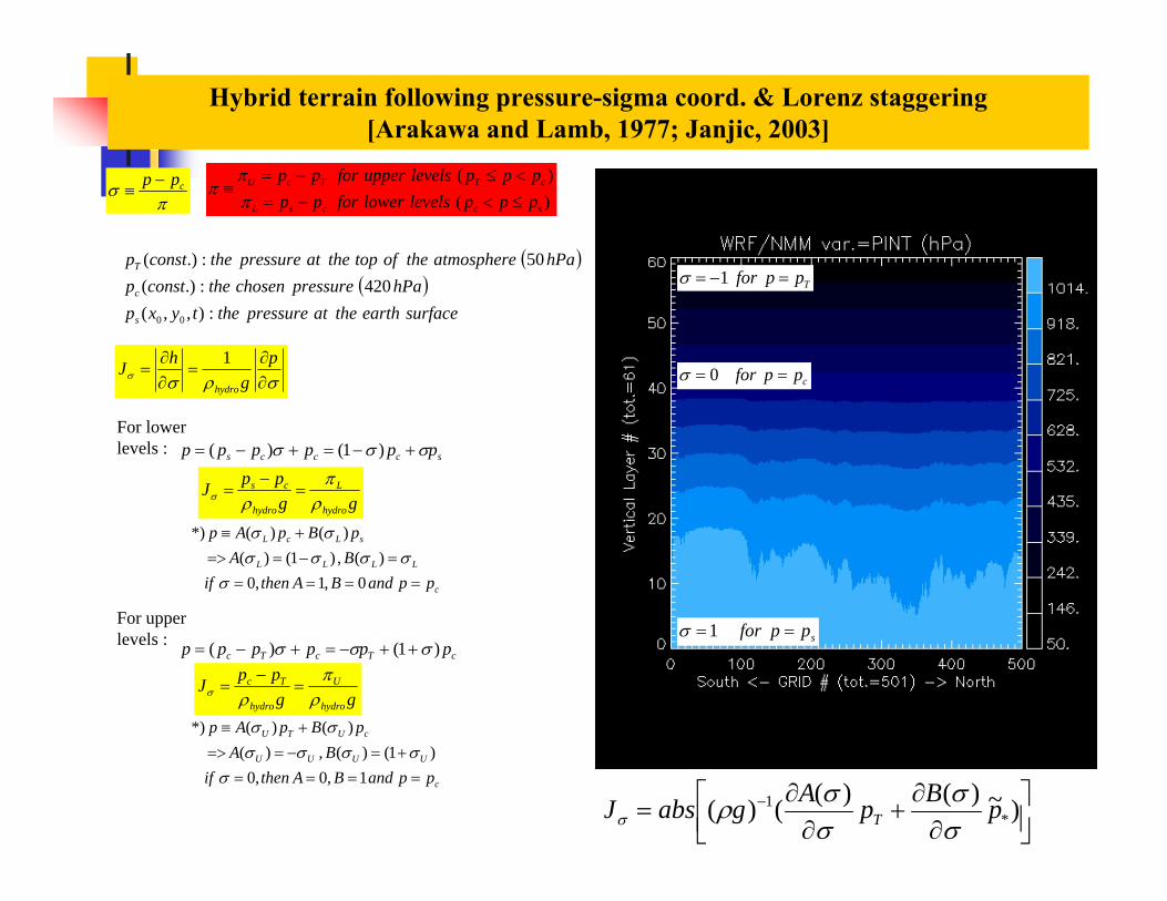
πσ cpp −

≡ )()(

sccsL

cTTcU

ppplevelslowerforppppplevelsupperforpp

≤<−=<≤−=

≡ππ

π

( )( )

surfaceearththeatpressurethetyxphPapressurechosentheconstp

hPaatmospheretheoftoptheatpressuretheconstp

s

c

T

:),,(420:.)(

50:.)(

00

sppfor == 1σ

cppfor == 0σ

Tppfor =−= 1σ

σρσσ ∂∂

=∂∂

=p

ghJ

hydro

1

For lower levels : scccs pppppp σσσ +−=+−= )1()(

ggppJ

hydro

L

hydro

cs

ρπ

ρσ =−

=

For upper levels :

cTcTc pppppp )1()( σσσ ++−=+−=

ggppJ

hydro

U

hydro

Tc

ρπ

ρσ =−

=

c

LLLL

sLcL

ppandBAthenifBApBpAp

=====−==>

+≡

0,1,0)(,)1()(

)()(*)

σσσσσ

σσ

c

UUUU

cUTU

ppandBAthenifBA

pBpAp

====+=−==>

+≡

1,0,0)1()(,)(

)()(*)

σσσσσ

σσ

Hybrid terrain following pressure-sigma coord. & Lorenz staggering [Arakawa and Lamb, 1977; Janjic, 2003]

⎥⎦⎤

⎢⎣⎡

∂∂

+∂

∂= − )~)()(()( *

1 pBpAgabsJ T σσ

σσρσ

WRF/nmm Utilizes Rotated Latitude/Longitude Coordinate

( )( )

Λ =−

− +arctg

cos sincos cos cos sin sin

ϕ λ λϕ ϕ λ λ ϕ ϕ

0

0 0 0

( )( )Φ = − −arcsin cos sin sin cos cosϕ ϕ ϕ ϕ λ λ0 0 0

( )[ ] ( )( )[ ]2

000

00000

coscossinsincos1

sinsincossinsincoscos

λλϕϕϕϕ

λλϕλλϕϕϕϕ

−−−

−−−+=

vuU

( ) ( )[ ]( )[ ]

Vu v

=− + + −

− − −

sin sin cos cos sin sin cos

cos sin sin cos cos

ϕ λ λ ϕ ϕ ϕ ϕ λ λ

ϕ ϕ ϕ ϕ λ λ

0 0 0 0 0

0 0 02

1

( )( )

uU V

=− +

− +

cos cos sin sin cos sin sin

cos sin sin cos cos

ϕ ϕ ϕ

ϕ ϕ

0 0 0

0 021

Φ Φ Λ Λ

Φ Λ Φ

( )( )

vU V

=− + −

− +

sin sin cos cos sin sin cos

cos sin sin cos cos

ϕ ϕ ϕ

ϕ ϕ

0 0 0

0 021

Λ Φ Φ Λ

Φ Λ Φ

sytemcoordinatenaturaldomainofcenter

sytemcoordinaterotated

:),(:),(:),(

00

λϕλϕΦΛ

( )V = U,V

( )v = u,v

The horizontal wind in the rotated system

The horizontal wind in the natural latitude/longitude system

“The simplicity of a lat-lon grid is made applicable over the entire globe by rotating the earth’s lat-lon grid such that the equator and prime meridian intersect at the center of the WRF/nmm computational grid. This rotation minimizes the convergence of meridians, keeping the true horizontal scale relatively uniform over the domain” (Tom Black, 1988; Pyle et al.,2004)

Grid definition <griddef_08central> for the model domain of (223x502)DATA TLM0D/-98.0/, TPH0D/37.0/, WBD/-11.866370/, SBD/-13.157894/, DLMD/.053452115/, DPHD/.052631578/

Earth Lon./Lat. of Center Rotated Lon./Lat. of Left and Lower dXrotated/dXrotated (degree)

Calculate some information from <griddef_08central>

- LONrotated (i,j) & LATrotated (i,j) (radian) - LONearth (i,j) & LATearth (i,j) (radian)

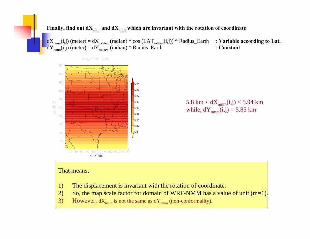
Finally, find out dXnmm and dXnmm which are invariant with the rotation of coordinate

dXnmm(i,j) (meter) = dXrotated (radian) * cos (LATrotated(i,j)) * Radius_Earth : Variable according to Lat.dYnmm(i,j) (meter) = dYrotated (radian) * Radius_Earth : Constant

That means;

1) The displacement is invariant with the rotation of coordinate.2) So, the map scale factor for domain of WRF-NMM has a value of unit (m=1).3) However, dXnmm is not the same as dYnmm (non-conformality).

5.8 km < dXnmm(i,j) < 5.94 km while, dYnmm(i,j) = 5.85 km

Horizontal Grid System of WRF/nmm:Rotated lat./long & Arakawa-E grid -> C-grid for CMAQ

If we use diamond gridC(C,R,L,S) -> C*(CR, L,S)

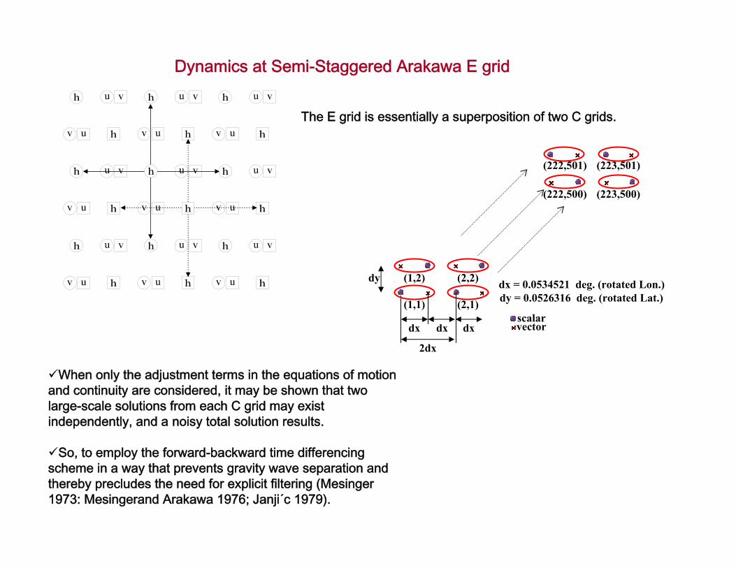
Dynamics at Semi-Staggered Arakawa E grid

The E grid is essentially a superposition of two C grids.

When only the adjustment terms in the equations of motion and continuity are considered, it may be shown that two large-scale solutions from each C grid may exist independently, and a noisy total solution results.

So, to employ the forward-backward time differencing scheme in a way that prevents gravity wave separation and thereby precludes the need for explicit filtering (Mesinger1973: Mesingerand Arakawa 1976; Janji´c 1979).

(1,1) (2,1)

(1,2) (2,2)

(223,501)

(223,500)

(222,501)

(222,500)

dx

dy

dx dx

dx = 0.0534521 deg. (rotated Lon.)dy = 0.0526316 deg. (rotated Lat.)

2dx

scalarvector

Semi-Staggered Arakawa E grid on the Rotated Lon./Lat. System

The momentum field (u-wind and v-wind) is computed on different points than the mass or scalar field (temperature, moisture, TKE, vertical wind, pressure and passive substants)

In order to achieve higher computational efficiency of the model code, the grid is rotated relative to other grid configurations (two horizontal coordinate systems in plane geometry, the main (x,y) and the auxiliary (x’,y’) system, both will be used in order to perform horizontal differencing )

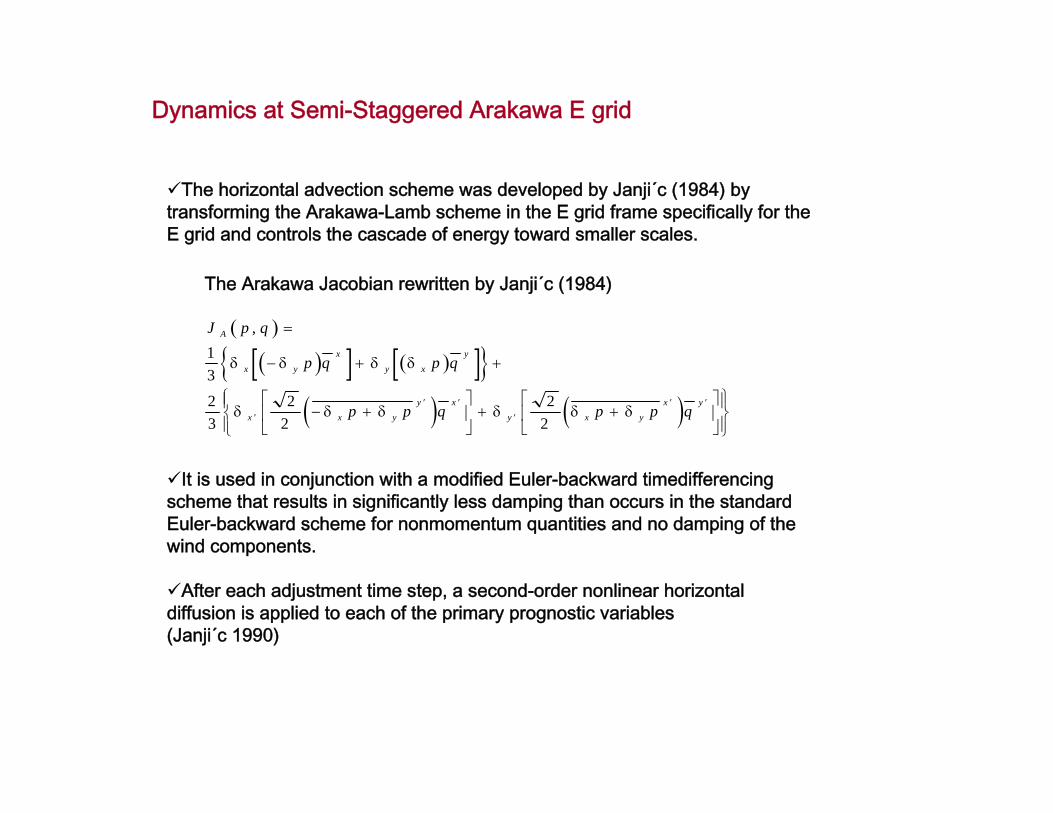
Dynamics at Semi-Staggered Arakawa E grid

The horizontal advection scheme was developed by Janji´c (1984) by transforming the Arakawa-Lamb scheme in the E grid frame specifically for the E grid and controls the cascade of energy toward smaller scales.

It is used in conjunction with a modified Euler-backward timedifferencingscheme that results in significantly less damping than occurs in the standard Euler-backward scheme for nonmomentum quantities and no damping of the wind components.

After each adjustment time step, a second-order nonlinear horizontal diffusion is applied to each of the primary prognostic variables(Janji´c 1990)

( )

( )[ ] ( )[ ] ( ) ( )

J p q

p q p q

p p q p p q

A

x y

x

y x

y

x x yy x

y x yx y

, =

− + +

− +⎡

⎣⎢

⎤

⎦⎥ + +

⎡

⎣⎢

⎤

⎦⎥

⎧⎨⎪

⎩⎪

⎫⎬⎪

⎭⎪′

′ ′

′

′ ′

1323

22

22

δ δ δ δ

δ δ δ δ δ δ

The Arakawa Jacobian rewritten by Janji´c (1984)

Dynamics at Semi-Staggered Arakawa E grid

Conservation properties

( ) ( ) ( ) ( ) ( )∂∂

δ δ δ δt

h u U u V u U u V uu xx x

yx y

xx x

yx y

= − +⎡⎣⎢

⎤⎦⎥

+ +⎡⎣⎢

⎤⎦⎥

⎧⎨⎩

⎫⎬⎭

+′

′

′

′′13

23

...

The conservation of the momentum

The conservation the kinetic energy

∂∂

δ δ δ δh u U uu V uu U uu V uux

x

x x

y

x y

x

x x

y

x y12

13

12

12

23

12

12

2⎛⎝⎜

⎞⎠⎟

= − ⎛⎝⎜

⎞⎠⎟

+ ⎛⎝⎜

⎞⎠⎟

⎡

⎣⎢

⎤

⎦⎥

⎛⎝⎜

⎞⎠⎟

+ ⎛⎝⎜

⎞⎠⎟

⎡

⎣⎢

⎤

⎦⎥

⎧⎨⎩

⎫⎬⎭+′

′

′

′

...

∂∂

δ δ δ δh v U vv V vv U vv V vvx

x

x x

y

x y

x

x x

y

x y12

13

12

12

23

12

12

2⎛⎝⎜

⎞⎠⎟

= − ⎛⎝⎜

⎞⎠⎟

+ ⎛⎝⎜

⎞⎠⎟

⎡

⎣⎢

⎤

⎦⎥

⎛⎝⎜

⎞⎠⎟

+ ⎛⎝⎜

⎞⎠⎟

⎡

⎣⎢

⎤

⎦⎥

⎧⎨⎩

⎫⎬⎭+′

′

′

′

...

After summation over a domain with cyclic boundary conditions, the right hand side of each equation vanishes,

and thus, the properties are conserved.

Dimension for Grid Point

(NCOL , NROW)(NCOL , NROW)(NCOL , NROW)For WRF/NMM

X-dir (NCOL+1 , NROW)Y-dir (NCOL , NROW+1)

(NCOL , NROW)(NCOL+1 , NROW+1)For WRF/EM (WCIP)

X-dir (NCOL+1 , NROW)Y-dir (NCOL , NROW+1)

(NCOL , NROW)(NCOL+1 , NROW+1)For MM5 (MCIP)

Flux-PointCross-PointDot-Point

Consistent coordinates and grid structuresWRF/EM & CMAQ utilize Arakawa-C Grid

Arakawa-B Grid (MM5) is linearly interpolated onto Arakawa-C Grid (CMAQ)

How to Utilize Arakawa-E for CMAQ?Develop a horizontal advection algorithm in CMAQ for Arakawa E-gridsSplit 2-D horizontal advection operator into 1-D operators and use CMAQ-proven 1-D schemes, such as PPM, with alternation between appropriate X and Y directionsWork directly with meteorological variables on the E-grid - avoid spatial interpolation

Option 1: Rotated square cells (rotated B-grid then on C-grid

Spatial distribution of dependent variables for a uniformly spaced Arakawa E-Grid

E-Grid with rotated square cells. Scalar variables are considered to be constant on each grid

Advantages Makes the E-Grid look like a B-grid whose “rows” and “columns” are along diagonal SW→NE and SE→NW linesCan use 1-D algorithm, e.g. PPM, along these linesCMAQ (and preprocessors) are familiar with turning B-grid data into C-grid flux point data

Disadvantages

Diagonal lines of cells have variable lengths, which requires non-trivial extra book-keeping (in EGRID_MODULE.F)Requires interpolation of wind velocities to get flux point valuesJagged boundary effectParallelization is more difficult

Grid geometry changes depending on whether thenumber of columns or rows is even or odd

Bookkeeping issues

Partitioning for parallelization

.

Cells have the same area as the rotated cells

E-grid wind velocity components are already at cell flux points – no interpolation neededSimpler book-keeping (but columns and row lengths can still vary by 1)Easier parallelization

Grid separation effect – DEAL KILLER(The sub-grid with odd numbered columns and rows and the sub-grid with even numbered columns and rows form two separate C-grids that don’t exchange mass by advection)Lower resolution (greater distance between cell centers) in the advection directionsNeed an extra E-grid column or row on each edge to get boundary conditions

Advantages

Disadvantages

Option 2: Rotated square cells (XY-Elongated cell)

Alternate between rotated cell advection and XY cell advection – mitigatesthe drawbacks of each method alone

Option 3: mixed grid

Jagged Boundary Effect

Boundary values propagate into the domain because boundaries are angled 45 degree

Option 1: rotated B-grid then on C-grid

Grid Separation Effect: signals moving x- and y-direction each do not interact

Option 2: XY-Elongated cellOption 1: rotated B-grid then on C-grid

Option 1: rotated B-grid then on C-gridCMAQ C-grid

Comparison between regular CMAQ and Option 1

Option 2: XY-Elongated cell Option 3: mixed grid

Comparison between Option 2 & 3

Variables required for linking WCIP and WRF-EM! Dynamics

:: u_m(:,:,:) ! U wind (m/s)

:: v_m(:,:,:) ! V wind (m/s)

:: w_m(:,:,:) ! W wind (m/s)

:: ww_mm(:,:,:)! Eta-dot (Pa s-1)

! Geopotential

:: ph_m(:,:,:) ! perturbation geopotential

:: phb_m(:,:,:) ! base-state geopotential

! Temperature

:: t_m(:,:,:) ! Temperature - 300 (K)

! Pressure

:: p_m(:,:,:) ! perturbation pressure [Pa]

:: pb_m(:,:,:) ! base-state pressure [Pa]

:: psfc_m(:,:) ! surface pressure [Pa]

! TKE

:: tke_m(:,:,:) ! turbulent kinetic energy

:: tke_myj_m(:,:,:) ! TKE in the MYJ scheme

! Water mixing ratio

:: qvapor_m(:,:,:) ! water vapoar [kg/kg]

:: qcloud_m(:,:,:) ! cloud water [kg/kg]

:: qrain_m(:,:,:) ! rain water [kg/kg]

:: qice_m(:,:,:) ! ice [kg/kg]

:: qsnow_m(:,:,:) ! snow [kg/kg]

! Density

:: alt_m(:,:,:) ! inverse density [m3 kg-1]

! 2D (J,I,ITIME)

:: mu_m(:,:) ! perturbation dry air mass in column [Pa]

:: mub_m(:,:) ! base-state dry air mass in column [Pa]

:: q2_m(:,:) ! QV at 2m [kg/kg]

:: t2_m(:,:) ! Temp at 2m [K]

:: th2_m(:,:) ! Pot. Temp. at 2m [K]

:: u10_m(:,:) ! U at 10 m [m/s]

:: v10_m(:,:) ! V at 10 m [m/s]

:: mapfac_m_m(:,:) ! map scale factor at cross

:: mapfac_u_m(:,:) ! map scale factor at square

:: mapfac_v_m(:,:) ! map scale factor at Triangle

:: hgt_m(:,:) ! Terrain height [m]

:: tsk_m(:,:) ! surface skin temperature [K]

:: sst_m(:,:) ! sea surface temp [K]

:: rainc_m(:,:) ! accumulated total CU precipitation [mm]

:: rainnc_m(:,:)! accumulated total Grid scale precip. [mm]

:: swdown_m(:,:) !sfc downward shortwave flux [W m-2]

:: gsw_m(:,:) ! sfc downdward shortwave flux [W m-2]

:: glw_m(:,:) ! sfc downdward longwave flux [W m-2]

:: xlat_m(:,:) ! latitude at cross [deg]

:: xlong_m(:,:) ! longitude at cross [deg]

:: lu_index_m(:,:) ! land use

:: hfx_m(:,:) ! sfc upward heat flux [W m-2]

:: qfx_m(:,:) ! sfc upward moisture flux [kg m-2 s-1]

:: snowc_m(:,:) ! snow cover (1=snow)

! add

:: mavail_m(:,:) ! surface moisture availability

:: hol_m(:,:) ! PBL height over M-O length [m/m]

:: ust_m(:,:) ! u* [m s-1]

:: zpbl_m(:,:) ! PBL height [m]

:: ivgtyp_m(:,:) ! dominant vegetation category

:: isltyp_m(:,:) ! dominant soil category

:: vegfra_m(:,:) ! vegetation fraction

:: canwat_m(:,:) ! canopy water [kg m-2]

:: albedo_m(:,:) ! albedo

:: emiss_m(:,:) ! surface emissivity

:: znt_m(:,:) ! surface roughness length [m]

! 1D (K,ITIME)

:: znu_m(:)

:: znw_m(:)

! ...

! 1D (E,ITIME) ---> E: ext_scalar

:: p_top

:: itimestep

:: mp_physics

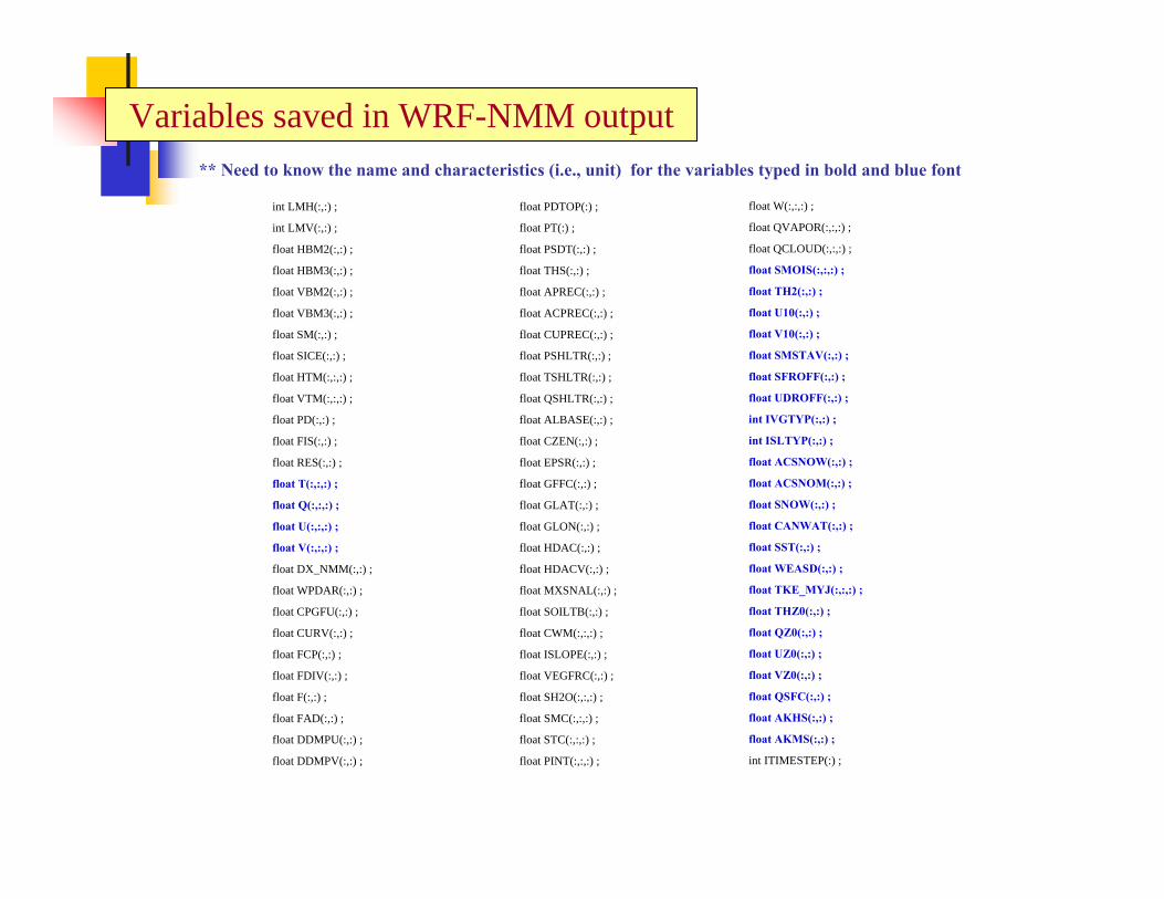
Variables saved in WRF-NMM output

int LMH(:,:) ;

int LMV(:,:) ;

float HBM2(:,:) ;

float HBM3(:,:) ;

float VBM2(:,:) ;

float VBM3(:,:) ;

float SM(:,:) ;

float SICE(:,:) ;

float HTM(:,:,:) ;

float VTM(:,:,:) ;

float PD(:,:) ;

float FIS(:,:) ;

float RES(:,:) ;

float T(:,:,:) ;

float Q(:,:,:) ;

float U(:,:,:) ;

float V(:,:,:) ;

float DX_NMM(:,:) ;

float WPDAR(:,:) ;

float CPGFU(:,:) ;

float CURV(:,:) ;

float FCP(:,:) ;

float FDIV(:,:) ;

float F(:,:) ;

float FAD(:,:) ;

float DDMPU(:,:) ;

float DDMPV(:,:) ;

float PDTOP(:) ;

float PT(:) ;

float PSDT(:,:) ;

float THS(:,:) ;

float APREC(:,:) ;

float ACPREC(:,:) ;

float CUPREC(:,:) ;

float PSHLTR(:,:) ;

float TSHLTR(:,:) ;

float QSHLTR(:,:) ;

float ALBASE(:,:) ;

float CZEN(:,:) ;

float EPSR(:,:) ;

float GFFC(:,:) ;

float GLAT(:,:) ;

float GLON(:,:) ;

float HDAC(:,:) ;

float HDACV(:,:) ;

float MXSNAL(:,:) ;

float SOILTB(:,:) ;

float CWM(:,:,:) ;

float ISLOPE(:,:) ;

float VEGFRC(:,:) ;

float SH2O(:,:,:) ;

float SMC(:,:,:) ;

float STC(:,:,:) ;

float PINT(:,:,:) ;

float W(:,:,:) ;

float QVAPOR(:,:,:) ;

float QCLOUD(:,:,:) ;

float SMOIS(:,:,:) ;

float TH2(:,:) ;

float U10(:,:) ;

float V10(:,:) ;

float SMSTAV(:,:) ;

float SFROFF(:,:) ;

float UDROFF(:,:) ;

int IVGTYP(:,:) ;

int ISLTYP(:,:) ;

float ACSNOW(:,:) ;

float ACSNOM(:,:) ;

float SNOW(:,:) ;

float CANWAT(:,:) ;

float SST(:,:) ;

float WEASD(:,:) ;

float TKE_MYJ(:,:,:) ;

float THZ0(:,:) ;

float QZ0(:,:) ;

float UZ0(:,:) ;

float VZ0(:,:) ;

float QSFC(:,:) ;

float AKHS(:,:) ;

float AKMS(:,:) ;

int ITIMESTEP(:) ;

** Need to know the name and characteristics (i.e., unit) for the variables typed in bold and blue font

Summary

Issues related with linking WRF models with CMAQ discussed

Studied differences in the governing equations and coordinates, their interactions with transport algorithms in WRF and the CMAQchemistry-transport model

Presented several methods to cast the WRF meteorological data onCMAQ grid and coordinate structures to represent transportation of pollutants.

Contrasted the differences in dynamics descriptions between the WRF/NMM and WRF/EM and their implication on the development of the linking strategy.