coupling of vertical and horizontal transport models · the danish environmental protection agency...
TRANSCRIPT
GrundRisk Coupling of vertical and
horizontal transport models
Environmental Project No. 1915 January 2017

2 The Danish Environmental Protection Agency / GrundRisk / Coupling of vertical and horizontal transport models
Publisher: The Danish Environmental Protection Agency
Editors:
Luca Locatelli, DTU Miljø
Louise Rosenberg, DTU Miljø
Poul L. Bjerg, DTU Miljø
Philip J. Binning, DTU Miljø
ISBN: 978-87-93529-56-4
The Danish Environmental Protection Agency publishes reports and papers about research and development projects
within the environmental sector, financed by the Agency. The contents of this publication do not necessarily represent
the official views of the Danish Environmental Protection Agency. By publishing this report, the Danish Environmental
Protection Agency expresses that the content represents an important contribution to the related discourse on Danish
environmental policy.
Sources must be acknowledged.

The Danish Environmental Protection Agency / GrundRisk / Coupling of vertical and horizontal transport models 3
Content
Content 3
Preface 5
Konklusion og sammenfatning 6
Summary and Conclusion 8
1. Introduction 10
1.1 Aim of the project 11
1.2 Model outputs 12
1.3 Structure of the report 12
2. Description of the five contaminant transport models 13
2.1 Model I. Homogeneous saturated clay overlying an aquifer 14
2.1.1 Model I. Homogeneous saturated clay vertical contaminant transport model 15
2.1.2 Model I. Coupling between the horizontal and vertical model 16
2.1.3 Model I. Model parameters, variables and output 17
2.2 Model II. Fractured saturated clay overlying an aquifer 18
2.2.1 Model II. Vertical transport model within a saturated fracture clay. 19
2.2.2 Model II. Coupling between the horizontal and vertical model 21
2.2.3 Model II. Model parameters and output 22
2.3 Model III. Unsaturated zone overlying an unconfined aquifer 23
2.3.1 Model III. Unsaturated zone vertical transport model with infiltration 23
2.3.2 Model III. Coupling between the horizontal and vertical model 26
2.3.3 Model III. Model parameters and output 28
2.4 Model IV. Unsaturated zone under an impervious area with zero infiltration 28
2.4.1 Model IV. Unsaturated zone vertical transport model without infiltration 30
2.4.2 Model IV. Coupling between the horizontal and vertical model 30
2.4.3 Model IV. Model parameters and output 31
2.5 Model V. Direct input from the contaminant source to the groundwater aquifer 32
2.6 Incorporation of reactive decay chains 33
3. Model applications 34
3.1 Rugårdsvej. Application of Model I 34
3.1.1 Geology and hydrogeology 34
3.1.2 Contamination at the site 35
3.1.3 Conceptual model and parameters for Rugårdsvej 35
3.1.4 Results for Rugårdsvej 37
3.1.5 Rugårdsvej example assuming contamination of benzene and toluene 38
3.1.6 Conclusion of Model I application 40
3.2 Vadsbyvej. Application of model II 40
3.2.1 Geology and hydrogeology 40
3.2.2 Contamination at the site 41
3.2.3 Conceptual model and parameters for Vadsbyvej 42
3.2.4 Results for Vadsbyvej 43
3.2.5 The effect of the fracture spacing parameter 2B 44
3.2.6 The assumption of fully mixed conditions at the bottom of the fractured aquitard 45
3.2.7 Conclusion of Model II application 47

4 The Danish Environmental Protection Agency / GrundRisk / Coupling of vertical and horizontal transport models
3.3 MW Gjøes Vej. Application of model III 48
3.3.1 Geology and hydrogeology 48
3.3.2 Contamination at the site 48
3.3.3 Conceptual model and parameters for MW Gløes Vej 48
3.3.4 Results for MW Gjøes Vej 50
3.3.5 MW Gjøes Vej example assuming contamination of benzene and toluene 52
3.3.6 Determining the numerical integration intervals of Model III 53
3.3.7 Conclusion of Model III application 54
3.4 MW Gjøes Vej. Application of model IV 55
3.4.1 Determining the numerical integration intervals of Model IV. 56
3.4.2 Conclusion of Model IV application 57
References 58
Appendix I 61

The Danish Environmental Protection Agency / GrundRisk / Coupling of vertical and horizontal transport models 5
This report presents the development of the GrundRisk model for contaminated site risk as-
sessment. GrundRisk consists of 5 models, each simulating the contaminant transport from a
contaminant source to an underlying aquifer. Each model consist of a vertical transport model
(based on the models presented in Miljøstyrelsen (2016a)) coupled to a horizontal transport
model (Miljøstyrelsen (2016b). This report focuses on the coupling between the vertical and
horizontal models.
In order to achieve a more realistic risk assessment and prioritization of contaminated sites new
methods need to be developed. This report is part of the project GrundRisk, where DTU Envi-
ronment and Miljøstyrelsen (the Danish Environmental Protection Agency) have identified four
research goals to be addressed in four sub-projects:
1. Development of an effective method for risk screening of identified contaminated sites
(V1 and V2), so that contamination threatening groundwater resources is identified at
an early stage.
2. Development of computational models for risk assessment of contaminated sites
threatening groundwater resources. Based on an evaluation of the current risk as-
sessment (standard no. 6 and 7, the Miljøstyrelsen, 1998), a new and more realistic
model is developed for more detailed assessment following the initial risk screening.
3. Development of a methodology for prioritization of remediation measures in a ground-
water catchment or a larger geographical area.
4. Development of a method to assess the groundwater management strategy.
This report is part of sub-project 2.
Preface
6 The Danish Environmental Protection Agency / GrundRisk / Coupling of vertical and horizontal transport models
I denne rapport præsenteres fem nye modeller (Model I, II, III, IV og V) til risikovurdering af
forurenede grunde i Danmark. De nye modeller sammenkobler forskellige modeller for vertikal
forureningstransport til en horisontal model for transport af forurening i grundvandet. Modellerne
er baseret på stationære løsninger, og kan simulere forureningskoncentrationer under en foru-
reningskilde og nedstrøms i et kontrolpunkt i det underliggende grundvandsmagasin. Modeller-
ne er implementeret i MATLAB.
Denne rapport præsenterer de metoder, der er anvendt til at koble de vertikale og horisontale
transportmodeller. Desuden beskrives det hvilke antagelser, der er gjort, og der gøres rede for
baggrunden for de valgte metoder. Modellerne er desuden afprøvet på tre udvalgte testlokalite-
ter i Danmark for herigennem at demonstrere deres kunnen.
Ved anvendelse af de nye koblede modeller, der kobler den horisontale transportmodel
GrundRisk (Miljøstyrelsen, 2016b) med vertikale transportmodeller, fås lavere forureningskon-
centrationer i grundvandsmagasinet, end hvis den horisontale model anvendes alene. Dette
skyldes, at modellerne indeholder flere transportprocesser for den vertikale transport (dispersi-
on, nedbrydning mv.) under forureningens transport fra kilden til toppen af grundvandsmagasi-
net.
De nye modeller er en del af GrundRisk (Miljøstyrelsen, 2016b), som er et nyt risikovurderings-
værktøj, der har til formål at give en mere realistisk risikovurdering, der inkluderer de mest rele-
vante transportprocesser. Hermed bliver identifikationen af grundvandstruende forureninger
mere præcis, og indsatsen i forhold til videre undersøgelser og afværge af forurenede lokalite-
ter bliver mere målrettet.
Anvendelsen af modellerne på de tre testlokaliteter viser, at vertikale transportprocesser kan
have en betydelige indvirkning på de simulerede koncentrationer i det underliggende grund-
vandsmagasin, især når det gælder letnedbrydelige forureninger som eksempelvis benzen og
toluen. Testlokaliteten Rugårdsvej, hvor grundvandsmagasinet er overlejret af homogent mæt-
tet sand, viste, at den 6 m lange vertikale transportvej fra forureningskilden til toppen af maga-
sinet gav en koncentrationsreduktion for dichlorethylen (DCE), mens koncentrationer af ned-
brydningsproduktet vinylklorid (VC) forøgedes. På testlokaliteten Vadsbyvej er grundvandsma-
gasinet overlejret af sprækket og mættet ler. Her viste resultaterne et lille fald i forureningskon-
centrationerne under den 7 m lange vertikale transportvej fra forureningskilden til toppen af
grundvandsmagasinet. Dette skyldes, at vandets hastighed i sprækkerne er høj, hvorfor trans-
porttiden er lille og nedbrydningens omfang dermed også er lille. På lokaliteten MW Gjøes Vej
overlejres et frit grundvandsmagasin af en 18 m dyb umættet zone af sand. Her viste resulta-
terne, at der under transporten til grundvandsmagasinet sker en lille reduktion i forureningskon-
centrationer pga. gasdiffusion (der var ingen nedbrydning i den umættede zone). Denne testlo-
kalitet blev også anvendt til at simulere en hypotetisk forurening med letnedbrydelige forurenin-
ger (benzen og toluen). Dette eksempel viste, at der skete en betydelig reduktion i forurenings-
koncentrationerne under transporten i den 18 m lange umættede zone især på grund af ned-
brydning. Desuden blev der for MW Gjøes Vej simuleret en situation, hvor der antages ikke at
ske infiltration til grundvandsmagasinet på grund af befæstningen af arealet. Dette eksempel
illustrerede hvordan umættede og mættede transportprocesser påvirker forureningskoncentrati-
onerne, når der ikke er nogen infiltration. Særligt viser eksemplet, hvorledes der sker diffusion
af forureningen gennem kapillærzonen på grænsen mellem den umættede og den mættede
zone.
Konklusion og sammenfatning

The Danish Environmental Protection Agency / GrundRisk / Coupling of vertical and horizontal transport models 7
Det er desuden undersøgt hvorledes modellernes følsomhed er overfor ændringer i infiltration,
nedbrydningsrater og sprækkeafstande (som er blandt de mest betydende modelparametre).
Beregningstiden for at simulere forureningskoncentrationer i et specifikt punkt i grundvandsma-
gasinet er få sekunder for Model I, II og V, hvorimod den kan vare op til 5 minutter for Model III
og Model IV. Beregningstiden forøges næsten lineært med antallet af beregningspunkter i
grundvandsmagasinet. At beregne et koncentrationsprofil i grundvandsmagasinet med 10 be-
regningspunkter vil tage ca. 50 minutter (10 gange 5 minutter) for hvert forureningsstof i Model
III og Model IV (hvis der er en reaktionskæde med 4 stoffer vil det tage 4 gange 50 minutter).
De vertikale transportmodeller inkluderer de vigtigste processer, der påvirker transporten af
forurening fra kildeområdet til et underliggende grundvandsmagasin. Der kan tages højde for
forskellige typer af geologi. Resultaterne viser, at det er vigtigt at tage højde for den vertikale
transport for at beskrive forureningsstoffernes skæbne fra forureningskilden til grundvandsma-
gasinet. Det er især vigtigt at give den vertikale transport opmærksomhed, hvis der er tale om
forureningsstoffer, der nedbrydes forholdsvis let (f.eks. BTEX), mens det er mindre vigtigt for
stoffer, der nedbrydes i mindre grad som f.eks. klorerede opløsningsmidler.

8 The Danish Environmental Protection Agency / GrundRisk / Coupling of vertical and horizontal transport models
This report presents five new contaminant transport models (Model I, II, III, IV and V) for risk
assessment of contaminated sites in Denmark. The new models couple different vertical con-
taminant transport models to a horizontal transport model. The models are based on steady-
state solutions and can simulate the contaminant concentration below a contaminant source
and downstream at control points in an underlying groundwater aquifer. The models are imple-
mented in MATLAB.
This report presents the methods needed to couple the vertical and horizontal transport models,
describing the assumptions made and the rationale for the chosen methods. The report demon-
strates the capabilities of the new models by applying them to three selected case studies in
Denmark.
The coupling between the horizontal transport model of GrundRisk (Miljøstyrelsen, 2016b) with
vertical transport models produces a reduction in the modeled concentrations in the aquifer
compared to the use of the horizontal transport alone. This is because of the added transport
processes (dispersion, degradation, etc.) in the vertical direction from the contaminant source
downward to the top of the aquifer.
The new models are part of GrundRisk (Miljøstyrelsen, 2016b) which is a new risk assessment
tool that aims to achieve a more realistic risk assessment, including the most relevant transport
processes so that identification of groundwater threatening contaminant sources becomes more
precise and site remediation can be more targeted.
The model application to the Danish case studies shows that vertical transport processes can
have a significant impact on the simulated concentration in underlying aquifers, particularly for
highly degradable compounds such as benzene and toluene. The case study of Rugårdsvej
where the aquifer is overlain by homogeneous saturated clay showed that the 6 m long vertical
transport pathway from the source to the top of the aquifer reduced the initial concentrations of
Dichlorethylen (DCE), however it increased those of Vinylchlorid (VC) (a degradation product
formed from DCE). The case study of Vadsbyvej where the aquifer is overlain by fractured
saturated clay showed that the 7 m long vertical transport pathway from the source to the top of
the aquifer slightly reduces contaminant concentrations, because the water velocity in the frac-
tures is high and the time it takes for the contaminant to reach the top of the aquifer from the
source is short and thus the degradation is small. The case study of MW Gjøes Vej where the
unconfined aquifer is overlain by unsaturated sand showed that the 18 m long vertical transport
pathway from the source to the top of the aquifer slightly reduces contaminant concentrations
due to gas diffusion (there was no degradation in the unsaturated zone). The case study of MW
Gjøes Vej was also used to simulate a hypothetical scenario with highly degradable compounds
(benzene and toluene) showing that the 18 m long vertical transport pathway from the source to
the top of the aquifer significantly reduces contaminant concentrations mainly due to degrada-
tion. Furthermore, the case study of MW Gjøes Vej was simulated assuming no recharge in the
area due to impervious surfaces covering the area. This scenario showed how unsaturated and
saturated transport processes affect the contaminant concentrations when there is no recharge,
particularly how the contaminant diffuses through the capillary fringe at the interface between
the unsaturated and the saturated zone.
Summary and Conclusion

The Danish Environmental Protection Agency / GrundRisk / Coupling of vertical and horizontal transport models 9
This report examined the model sensitivity to the model parameters: recharge rates, the first
order degradation rates and fracture spacing (which are among the most influential model pa-
rameters).. The computational time to simulate the contaminant concentration at a single point
in the aquifer is in the order of seconds for Model I, II and V, whereas it can be up to 5 minutes
for Model III and Model IV. The computational time increases almost linearly with the number of
simulated points in the aquifer, i.e. computing a concentration profile in the aquifer using 10
simulated points takes approximately 50 minutes (10 times 5 minutes) for each compound in
Model III and Model IV (if there is a reaction chain of 4 compounds it will take 4 times 50
minutes).
The vertical transport model includes the main processes affecting contaminant transport from
a source to an underlying groundwater aquifer. Various types of geology are considered. Con-
sideration of vertical transport is shown to be important for determining the attenuation of con-
taminant transport between the source and the underlying aquifer. Attenuation during vertical
transport is particularly important for more degradable compounds like BTEX, but has less
effect for less degradable compounds like the chlorinated solvents.
10 The Danish Environmental Protection Agency / GrundRisk / Coupling of vertical and horizontal transport models
1. Introduction
Risk assessments of contaminated sites are often conducted using simple models to determine
contaminant concentrations in groundwater downstream of the contaminant source. In Denmark
the JAGG model developed by Miljøstyrelsen (1998) and later updated (Miljøstyrelsen 2013) is
widely used for risk assessments of contaminated sites. The JAGG model simulates the con-
taminant concentration at a point of compliance based on input source concentrations and
geometry and other soil and groundwater parameters. JAGG is based on a simple 1-D model
with many simplifying assumptions, and is usually employed assuming a worst case scenario.
As a result of the conservative assumptions made, a large number of contaminant point
sources have been identified as a potential problem for groundwater. Hence there is a need for
improved models.
GrundRisk (Miljøstyrelsen, 2016b) is a new risk assessment tool that aims to achieve a more
realistic risk assessment including the most relevant transport processes so that identification of
groundwater threatening sources becomes more precise and site remediation can be more
targeted.
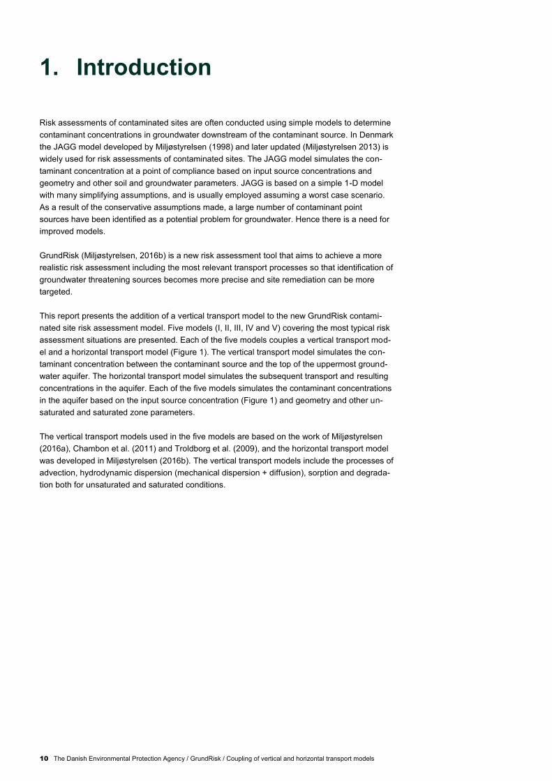
This report presents the addition of a vertical transport model to the new GrundRisk contami-
nated site risk assessment model. Five models (I, II, III, IV and V) covering the most typical risk
assessment situations are presented. Each of the five models couples a vertical transport mod-
el and a horizontal transport model (Figure 1). The vertical transport model simulates the con-
taminant concentration between the contaminant source and the top of the uppermost ground-
water aquifer. The horizontal transport model simulates the subsequent transport and resulting
concentrations in the aquifer. Each of the five models simulates the contaminant concentrations
in the aquifer based on the input source concentration (Figure 1) and geometry and other un-
saturated and saturated zone parameters.
The vertical transport models used in the five models are based on the work of Miljøstyrelsen
(2016a), Chambon et al. (2011) and Troldborg et al. (2009), and the horizontal transport model
was developed in Miljøstyrelsen (2016b). The vertical transport models include the processes of
advection, hydrodynamic dispersion (mechanical dispersion + diffusion), sorption and degrada-
tion both for unsaturated and saturated conditions.
The Danish Environmental Protection Agency / GrundRisk / Coupling of vertical and horizontal transport models 11
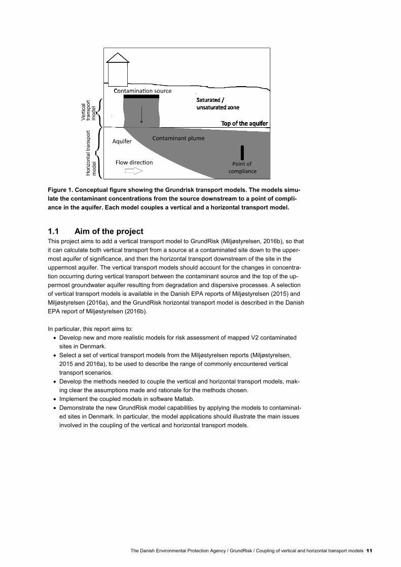
Figure 1. Conceptual figure showing the Grundrisk transport models. The models simu-
late the contaminant concentrations from the source downstream to a point of compli-
ance in the aquifer. Each model couples a vertical and a horizontal transport model.
1.1 Aim of the project This project aims to add a vertical transport model to GrundRisk (Miljøstyrelsen, 2016b), so that
it can calculate both vertical transport from a source at a contaminated site down to the upper-
most aquifer of significance, and then the horizontal transport downstream of the site in the
uppermost aquifer. The vertical transport models should account for the changes in concentra-
tion occurring during vertical transport between the contaminant source and the top of the up-
permost groundwater aquifer resulting from degradation and dispersive processes. A selection
of vertical transport models is available in the Danish EPA reports of Miljøstyrelsen (2015) and
Miljøstyrelsen (2016a), and the GrundRisk horizontal transport model is described in the Danish
EPA report of Miljøstyrelsen (2016b).
In particular, this report aims to:
Develop new and more realistic models for risk assessment of mapped V2 contaminated
sites in Denmark.
Select a set of vertical transport models from the Miljøstyrelsen reports (Miljøstyrelsen,
2015 and 2016a), to be used to describe the range of commonly encountered vertical
transport scenarios.
Develop the methods needed to couple the vertical and horizontal transport models, mak-
ing clear the assumptions made and rationale for the methods chosen.
Implement the coupled models in software Matlab.
Demonstrate the new GrundRisk model capabilities by applying the models to contaminat-
ed sites in Denmark. In particular, the model applications should illustrate the main issues
involved in the coupling of the vertical and horizontal transport models.

12 The Danish Environmental Protection Agency / GrundRisk / Coupling of vertical and horizontal transport models
1.2 Model outputs The new models simulate the contaminant water phase concentration from the source to the
top of the aquifer and then horizontally downstream in the aquifer. Figure 2 shows examples of
the output that can be obtained from the models simulating a contaminated site. Figure 2 (a)
shows the simulated concentrations from the source to the top of the aquifer; Figure 2 (b)
shows the simulated concentrations in the aquifer at a 0.01 m depth below the top of the aquifer
(concentration along the centerline of the plume can also be plotted) and Figure 2 (c) shows the
concentrations in the aquifer as a function of depth below the top of the aquifer, 100 m down-
stream the most downstream point of the source.
Figure 2. (a) Concentration as a function of the depth from the bottom of the source to
the top of the aquifer. (b) Concentration in the aquifer as a function of the distance
downstream of the source at a 0.01 m distance from the top of the aquifer. (c) Concentra-
tion in the aquifer at the centre of the plume 100 m downstream of the source.
1.3 Structure of the report The report is organized as follows;
Chapter 2 describes the details of the 5 different contaminant transport models. Conceptual
model, mathematical description, coupling approach and an overview of the model parame-
ters are given for each of the models.
Chapter 3 presents the model applications to different case studies.
A first time reader of this report may wish to skip the mathematical details in chapter 2 and
focus on the figures and conceptual descriptions of the models in chapter 2 and the model
applications in chapter 3.
-4
-3
-2
-1
0
0 0.1 0.2 0.3
De
pth
bel
ow
th
e
gro
un
dw
ate
r ta
ble
[m
]
Concentration 100 m downstream the source [mg/L]
(c)
0
1
2
3
4
5
-30 0 30 60 90 120
Co
nce
ntr
atio
n [
mg/
L]
Distance along the aquifer [m]
Source
(b)
-18
-15
-12
-9
-6
-3
0
0 10 20 30 40 50
De
pth
bel
ow
th
e so
urc
e [m
]
Concentration [mg/L]
(a)
The Danish Environmental Protection Agency / GrundRisk / Coupling of vertical and horizontal transport models 13
2. Description of the five contaminant transport models
This chapter describes the five different GrundRisk contaminant transport models (Model I, II,
III, IV and V). Each model consists of a coupled vertical and a horizontal transport model simu-
lating the transport from source to a point of compliance located in the aquifer downstream of
the source zone. The vertical transport model equations and the coupling model between the
vertical and horizontal transport components are described. A detailed description of the hori-
zontal transport model can be found in Miljøstyrelsen (2016b). The five different models aim to
include the most common contaminant transport mechanisms and processes of contaminated
sites. Table 1 shows a summary of the five contaminant transport models.
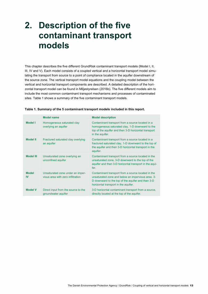
Table 1. Summary of the 5 contaminant transport models included in this report.
Model name Model description
Model I Homogeneous saturated clay
overlying an aquifer Contaminant transport from a source located in a
homogeneous saturated clay, 1-D downward to the
top of the aquifer and then 3-D horizontal transport
in the aquifer.
Model II Fractured saturated clay overlying
an aquifer Contaminant transport from a source located in a
fractured saturated clay, 1-D downward to the top of
the aquifer and then 3-D horizontal transport in the
aquifer.
Model III Unsaturated zone overlying an
unconfined aquifer Contaminant transport from a source located in the
unsaturated zone, 3-D downward to the top of the
aquifer and then 3-D horizontal transport in the aqui-
fer.
Model
IV Unsaturated zone under an imper-
vious area with zero infiltration Contaminant transport from a source located in the
unsaturated zone and below an impervious area, 3-
D downward to the top of the aquifer and then 3-D
horizontal transport in the aquifer.
Model V Direct input from the source to the
groundwater aquifer 3-D horizontal contaminant transport from a source,
directly located at the top of the aquifer.
14 The Danish Environmental Protection Agency / GrundRisk / Coupling of vertical and horizontal transport models
The choice of model is based on a conceptualization of the contaminant site which is outside
the scope of this report. Each model is based on an analytical steady state solution of the 3-
dimensional advection-dispersion equation and includes the most relevant transport processes
for that specific case.
All the models are based on the following assumptions:
Homogenous conditions. This means that the soil parameters (e.g. water content, porosity,
bulk density, content of organic carbon and dispersivity) and contaminant parameters (e.g.
diffusion coefficient, Henry’s law constant and degradation rates) are constant in space and
time.
Linear, reversible, instantaneous equilibrium sorption processes between the water and
solid phases
Advection only occurs in the water phase and in one dimension (the vertical and/or horizon-
tal flow direction) with a constant velocity.
Degradation is described by 1st order kinetics and occurs in only the water phase.
The concentration and the contaminant mass discharge in the contaminant source are con-
stant over time.
Transport of non-aqueous phase liquids is not included and the model only simulates dis-
solved compounds.
These assumptions/limitations are thought to be reasonable since the models are risk assess-
ment tools and not advanced solute transport models. In order to ensure that the model can be
used in risk assessments where little data is available, the conceptual models must be simple
and the input parameters must be few and well-known.
Each model employs a different coordinate system in order to develop the needed analytical
solution. Model I, II and V place the coordinate system origin on the upstream edge of the con-
taminant source, whereas Model III and IV place the origin at the center of the contaminant
source.
2.1 Model I. Homogeneous saturated clay overlying an aquifer The conceptual model for Model I is shown in Figure 3. Model I simulates the water phase con-
centrations in a saturated clay between the contaminant source and an underlying aquifer using
a vertical transport model, and then the concentrations in the underlying aquifer using a hori-
zontal transport model. The contaminant source is considered to have length Lx, width Ly, and a
source concentration of C0. The source can be located below land surface and has a user spec-
ified distance to the top of the aquifer. The vertical transport model of Model I simulates the
concentrations between the contaminant source and the top of the aquifer using a 1D steady-
state analytical solution that assumes that the horizontal mixing (dispersion) is negligible (i.e.
there is no variation in concentrations in the y and x directions of the vertical transport).
The output of the vertical transport model is the concentration C1 at the top of the aquifer. The
concentration C1 is used as input to the horizontal model computing downstream concentrations
in the aquifer. In the horizontal transport model, the concentration C1 is applied over the same
area (LxLy) as used in the source area. The horizontal model simulates the concentrations in the
aquifer based on a 3D steady-state analytical solution that includes advection and dispersion in
the aquifer. A complete description of the horizontal transport model is found in Miljøstyrelsen
(2016b). The following 3 sections describe the vertical transport component of Model I, the
coupling between the vertical and the horizontal transport models, and the model parameters.

The Danish Environmental Protection Agency / GrundRisk / Coupling of vertical and horizontal transport models 15
Figure 3. Conceptual Model I. Vertical contaminant transport from a source located in a
HOMOGENEOUS saturated clay, downward to the top of the aquifer and then horizontal
transport in the aquifer.
2.1.1 Model I. Homogeneous saturated clay vertical contaminant
transport model
This section presents the steady-state analytical solution that is used for computing the vertical
transport in Model I. The clay layer in this case is saturated (Figure 3) and so there is no gas
transport. The most significant transport processes within a homogeneous saturated layer are
percolation (advection) of the contaminant with groundwater recharge; diffusion and mechanical
dispersion in the water phase; sorption; and degradation. Note that Figure 3 shows that the
water table is above the contaminant source. The model can also be used when the water table
is below the source because the porous media will still be saturated above the aquifer due to
capillary rise in the low permeability material.
The transport equation for Model I is (Miljøstyrelsen, 2016a):
2w ww w w
C CR D C v C
t z
t TIME
FIRST ORDER DEGRADATION RATE
CW CONCENTRATION IN THE WATER PHASE
Z VERTICAL DISTANCE FROM THE SOURCE
V PORE WATER VELOCITY IN THE Z DIRECTION
R RETARDATION FACTOR
DW HYDRODYNAMIC DISPERSION COEFFICIENT IN WATER
Equation 1
The one-dimensional steady-state solution is shown in Equation 1 (van Genuchten et al., 1982).
It is noted that the retardation factor R does not affect the steady-state vertical transport. How-
ever, it can affect contaminant concentration at the top of the aquifer where the output of the
vertical transport model is input into the horizontal transport model (see Appendix I). This solu-
tion was found by applying the boundary conditions of fixed concentration at the source c(0)=Co
and zero gradient at infinite distance from the source dc/dz(∞)=0. The 1D solution has been
shown to be a good approximation of the 3D solution (Miljøstyrelsen, 2016a) because trans-
verse dispersion is negligible in saturated clay. Equation 2 is used to calculate the water phase
concentration at the top of the uppermost aquifer underlying the source. This concentration is
then used as input to the horizontal transport model.
16 The Danish Environmental Protection Agency / GrundRisk / Coupling of vertical and horizontal transport models
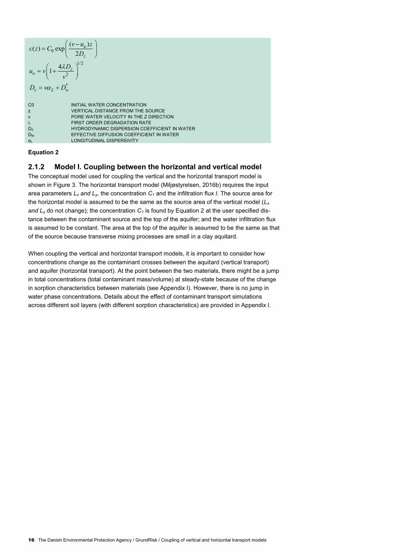
0
( )( ) exp
2
u
z
v u zc z C
D
1/2
2
41 z
u
Du v
v
*z L wD v D
C0 INITIAL WATER CONCENTRATION
z VERTICAL DISTANCE FROM THE SOURCE
v PORE WATER VELOCITY IN THE Z DIRECTION
FIRST ORDER DEGRADATION RATE
DZ HYDRODYNAMIC DISPERSION COEFFICIENT IN WATER
DW EFFECTIVE DIFFUSION COEFFICIENT IN WATER
αL LONGITUDINAL DISPERSIVITY
Equation 2
2.1.2 Model I. Coupling between the horizontal and vertical model
The conceptual model used for coupling the vertical and the horizontal transport model is
shown in Figure 3. The horizontal transport model (Miljøstyrelsen, 2016b) requires the input
area parameters Lx and Ly, the concentration C1 and the infiltration flux I. The source area for
the horizontal model is assumed to be the same as the source area of the vertical model (Lx
and Ly do not change); the concentration C1 is found by Equation 2 at the user specified dis-
tance between the contaminant source and the top of the aquifer; and the water infiltration flux
is assumed to be constant. The area at the top of the aquifer is assumed to be the same as that
of the source because transverse mixing processes are small in a clay aquitard.
When coupling the vertical and horizontal transport models, it is important to consider how
concentrations change as the contaminant crosses between the aquitard (vertical transport)
and aquifer (horizontal transport). At the point between the two materials, there might be a jump
in total concentrations (total contaminant mass/volume) at steady-state because of the change
in sorption characteristics between materials (see Appendix I). However, there is no jump in
water phase concentrations. Details about the effect of contaminant transport simulations
across different soil layers (with different sorption characteristics) are provided in Appendix I.

The Danish Environmental Protection Agency / GrundRisk / Coupling of vertical and horizontal transport models 17
2.1.3 Model I. Model parameters, variables and output
Table 2 shows the user input model parameters and Table 3 the derived variables for Model I.
The input parameters and variables in the tables are divided into three categories: Global pa-
rameters applicable to both the vertical and the horizontal transport model, Vertical model pa-
rameters, and Horizontal Model parameters. The model output is the contaminant concentration
at a single or multiple user specified points in the underlying aquifer.
Table 2. User input parameters of Model I
Input parameter
Description
Global parameters
Yi [-]* Stoichiometric ratio of each compound i of the degradation chain
I [L/T] Recharge
Lx [L] Source length
Ly [L] Source width
Vertical model
C0_v [M/L3] Concentration in the water phase at the source
k_v [T-1] First order degradation rate
n_v [-] Porosity = water content (assuming full water saturation)
αL_v [L] Longitudinal dispersivity (z direction)
Z_v [L] Distance between the source and the top of the aquifer
Dw_v [L2/T] Free diffusion coefficient in water
Horizontal model
H [L] Thickness of the aquifer
u [L/T] Groundwater velocity
k [T-1
] First order degradation rate
n [-] Porosity
αL [L] Longitudinal dispersivity (x direction)
αT [L] Transversal dispersivity (y direction)
αV [L] Vertical dispersivity (z direction)
* Yi+1=molar massi/molar mass
i+1. It is the ratio of the molar masses of the com-
pounds in a degradation chain.
Table 3. Derived variables for Model I.
Derived variables
Description
Vertical model _ v
Iv
n Pore water velocity
*_ _w v w vD D Effective diffusion coefficient in water (Bear, 1972)
Tortuosity of the soil matrix. Assumed to equal to the soil porosity as a first approximation (Parker et al., 1994)
Horizontal model
L LD u Longitudinal dispersion coefficient
T TD u Transversal dispersion coefficient
V VD u Vertical dispersion coefficient
18 The Danish Environmental Protection Agency / GrundRisk / Coupling of vertical and horizontal transport models
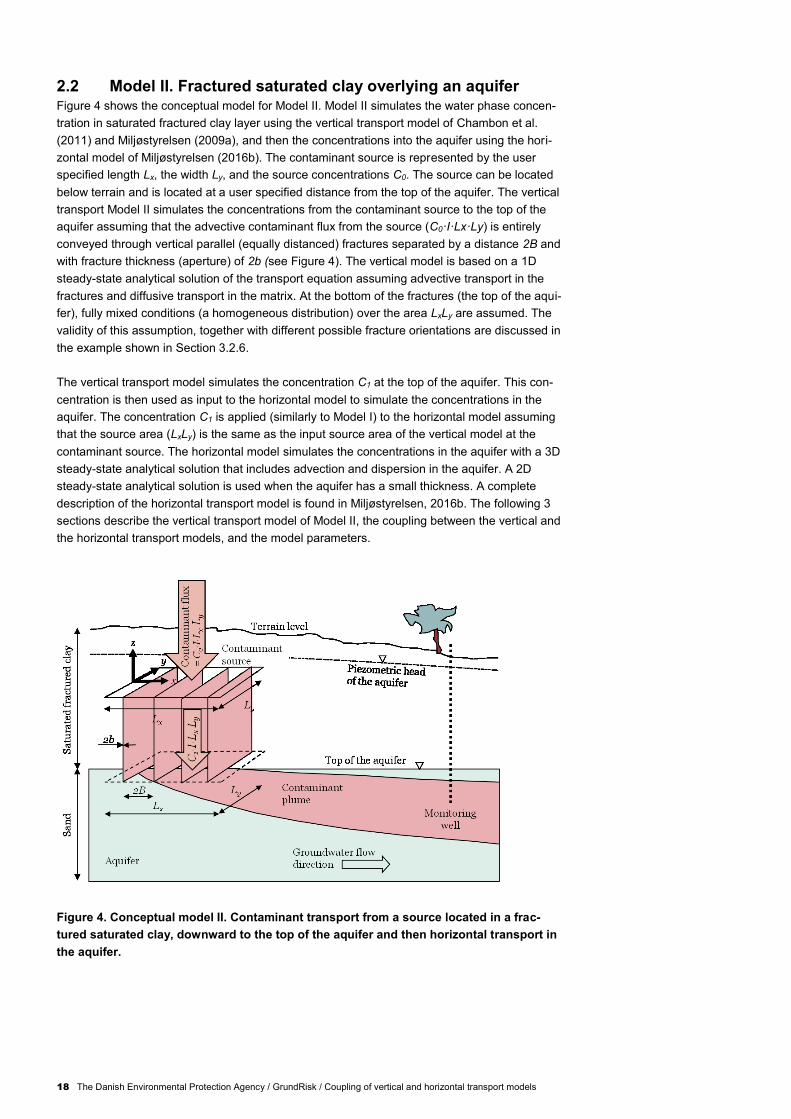
2.2 Model II. Fractured saturated clay overlying an aquifer Figure 4 shows the conceptual model for Model II. Model II simulates the water phase concen-
tration in saturated fractured clay layer using the vertical transport model of Chambon et al.
(2011) and Miljøstyrelsen (2009a), and then the concentrations into the aquifer using the hori-
zontal model of Miljøstyrelsen (2016b). The contaminant source is represented by the user
specified length Lx, the width Ly, and the source concentrations C0. The source can be located
below terrain and is located at a user specified distance from the top of the aquifer. The vertical
transport Model II simulates the concentrations from the contaminant source to the top of the
aquifer assuming that the advective contaminant flux from the source (C0·I·Lx·Ly) is entirely
conveyed through vertical parallel (equally distanced) fractures separated by a distance 2B and
with fracture thickness (aperture) of 2b (see Figure 4). The vertical model is based on a 1D
steady-state analytical solution of the transport equation assuming advective transport in the
fractures and diffusive transport in the matrix. At the bottom of the fractures (the top of the aqui-
fer), fully mixed conditions (a homogeneous distribution) over the area LxLy are assumed. The
validity of this assumption, together with different possible fracture orientations are discussed in
the example shown in Section 3.2.6.
The vertical transport model simulates the concentration C1 at the top of the aquifer. This con-
centration is then used as input to the horizontal model to simulate the concentrations in the
aquifer. The concentration C1 is applied (similarly to Model I) to the horizontal model assuming
that the source area (LxLy) is the same as the input source area of the vertical model at the
contaminant source. The horizontal model simulates the concentrations in the aquifer with a 3D
steady-state analytical solution that includes advection and dispersion in the aquifer. A 2D
steady-state analytical solution is used when the aquifer has a small thickness. A complete
description of the horizontal transport model is found in Miljøstyrelsen, 2016b. The following 3
sections describe the vertical transport model of Model II, the coupling between the vertical and
the horizontal transport models, and the model parameters.
Figure 4. Conceptual model II. Contaminant transport from a source located in a frac-
tured saturated clay, downward to the top of the aquifer and then horizontal transport in
the aquifer.

The Danish Environmental Protection Agency / GrundRisk / Coupling of vertical and horizontal transport models 19
2.2.1 Model II. Vertical transport model within a saturated fracture clay.
The vertical transport model of Model II calculates the downward vertical contaminant transport
in a saturated fractured clay from the source to the top of the underlying aquifer in a saturated
fractured clay. The model was presented by Chambon et al. (2011). The contaminant transport
in fractured clays is controlled by advection in the fractures and diffusion in the matrix (Cham-
bon et al., 2011). Contamination in both the fractures and the matrix is affected by both sorption
and degradation (Jørgensen et al., 2004; McKay et al., 1993; Broholm et al., 2000).
Several different mathematical models describing the contaminant transport in fractured media
are described by Chambon et al. (2011). Model II employs the model with a constant source
concentration above the fractured soil (Chambon et al. 2011). The vertical transport model used
in Model II is illustrated in Figure 5; this model simulates the steady-state concentration in the
fractured clay from a source with constant concentration C0. The mathematical model is based
on the following assumptions (in addition to those already mentioned in the introduction to
Chapter 2): mass transport along the fracture is one-dimensional; dispersion along the fracture
is neglected; advection in the porous matrix is neglected; transport in the matrix is perpendicu-
lar to the fracture. The mathematical solution was developed for an infinitly long single fracture
conveying the water flux over on infinitely long strip of width 2B.
Figure 5. Conceptual sketch of the vertical model of model II. source overlying the frac-
tured media for an infinite time (Chambon et al., 2011). C0 is the input concentration, cl is
the initial concentration in the matrix, 2b is the fracture spacing and 2b is the fracture
aperture. the red area represents the source above the fractured clay (modified from
Chambon et al., 2011).
The one-dimensional transport equation in a vertical fracture is shown in Equation 3 (Tang et
al., 1981). Advective transport is only considered in the fractures since there is little advection in
the matrix. This approximation is reasonable if the hydraulic conductivity of the matrix is low
compared to the hydraulic conductivity of the fracture.
0f f m
f f f
C C QR v C
t z b
t TIME
FIRST ORDER DEGRADATION RATE
Cf CONCENTRATION IN THE WATER PHASE IN A FRACTURE
z VERTICAL DISTANCE FROM THE SOURCE
vf WATER VELOCITY IN THE FRACTURE
Rf RETARDATION FACTOR ON THE FRACTURE SURFACE
Qm MASS TRANSFER FLUX AT THE FRACTURE-MATRIX INTERFACE [M/T/L2]
b HALF APERTURE OF THE FRACTURE
Equation 3
20 The Danish Environmental Protection Agency / GrundRisk / Coupling of vertical and horizontal transport models
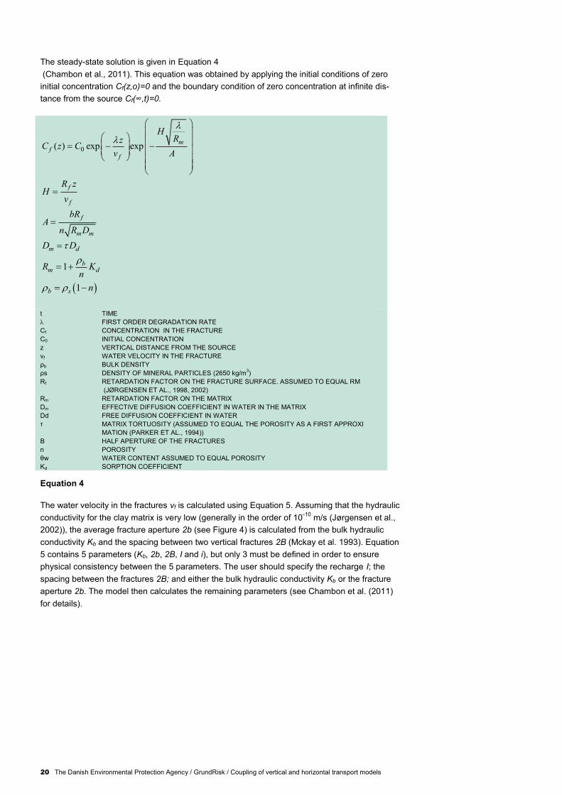
The steady-state solution is given in Equation 4
(Chambon et al., 2011). This equation was obtained by applying the initial conditions of zero
initial concentration Cf(z,o)=0 and the boundary condition of zero concentration at infinite dis-
tance from the source Cf(∞,t)=0.
0( ) exp expm
ff
HRz
C z Cv A
f
f
R zH
v
f
m m
bRA
n R D
m dD D
1 bm dR K
n
1b s n
t TIME
FIRST ORDER DEGRADATION RATE
Cf CONCENTRATION IN THE FRACTURE
C0 INITIAL CONCENTRATION
z VERTICAL DISTANCE FROM THE SOURCE
vf WATER VELOCITY IN THE FRACTURE
ρb BULK DENSITY
ρs DENSITY OF MINERAL PARTICLES (2650 kg/m3)
Rf RETARDATION FACTOR ON THE FRACTURE SURFACE. ASSUMED TO EQUAL RM
(JØRGENSEN ET AL., 1998, 2002)
Rm RETARDATION FACTOR ON THE MATRIX
Dm EFFECTIVE DIFFUSION COEFFICIENT IN WATER IN THE MATRIX
Dd FREE DIFFUSION COEFFICIENT IN WATER
τ MATRIX TORTUOSITY (ASSUMED TO EQUAL THE POROSITY AS A FIRST APPROXI
MATION (PARKER ET AL., 1994))
B HALF APERTURE OF THE FRACTURES
n POROSITY
θw WATER CONTENT ASSUMED TO EQUAL POROSITY
Kd SORPTION COEFFICIENT
Equation 4
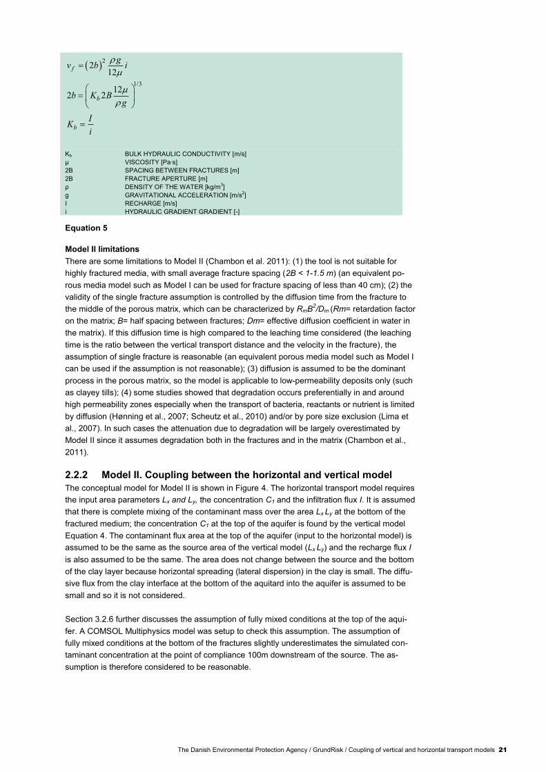
The water velocity in the fractures vf is calculated using Equation 5. Assuming that the hydraulic
conductivity for the clay matrix is very low (generally in the order of 10-10
m/s (Jørgensen et al.,
2002)), the average fracture aperture 2b (see Figure 4) is calculated from the bulk hydraulic
conductivity Kb and the spacing between two vertical fractures 2B (Mckay et al. 1993). Equation
5 contains 5 parameters (Kb, 2b, 2B, I and i), but only 3 must be defined in order to ensure
physical consistency between the 5 parameters. The user should specify the recharge I; the
spacing between the fractures 2B; and either the bulk hydraulic conductivity Kb or the fracture
aperture 2b. The model then calculates the remaining parameters (see Chambon et al. (2011)
for details).
The Danish Environmental Protection Agency / GrundRisk / Coupling of vertical and horizontal transport models 21
2
212
f
gv b i
1/312
2 2bb K Bg
b
IK
i
Kb BULK HYDRAULIC CONDUCTIVITY [m/s]
μ VISCOSITY [Pa∙s]
2B SPACING BETWEEN FRACTURES [m]
2B FRACTURE APERTURE [m]
ρ DENSITY OF THE WATER [kg/m3]
g GRAVITATIONAL ACCELERATION [m/s2]
I RECHARGE [m/s]
i HYDRAULIC GRADIENT GRADIENT [-]
Equation 5
Model II limitations
There are some limitations to Model II (Chambon et al. 2011): (1) the tool is not suitable for
highly fractured media, with small average fracture spacing (2B < 1-1.5 m) (an equivalent po-
rous media model such as Model I can be used for fracture spacing of less than 40 cm); (2) the
validity of the single fracture assumption is controlled by the diffusion time from the fracture to
the middle of the porous matrix, which can be characterized by RmB2/Dm (Rm= retardation factor
on the matrix; B= half spacing between fractures; Dm= effective diffusion coefficient in water in
the matrix). If this diffusion time is high compared to the leaching time considered (the leaching
time is the ratio between the vertical transport distance and the velocity in the fracture), the
assumption of single fracture is reasonable (an equivalent porous media model such as Model I
can be used if the assumption is not reasonable); (3) diffusion is assumed to be the dominant
process in the porous matrix, so the model is applicable to low-permeability deposits only (such
as clayey tills); (4) some studies showed that degradation occurs preferentially in and around
high permeability zones especially when the transport of bacteria, reactants or nutrient is limited
by diffusion (Hønning et al., 2007; Scheutz et al., 2010) and/or by pore size exclusion (Lima et
al., 2007). In such cases the attenuation due to degradation will be largely overestimated by
Model II since it assumes degradation both in the fractures and in the matrix (Chambon et al.,
2011).
2.2.2 Model II. Coupling between the horizontal and vertical model
The conceptual model for Model II is shown in Figure 4. The horizontal transport model requires
the input area parameters Lx and Ly, the concentration C1 and the infiltration flux I. It is assumed
that there is complete mixing of the contaminant mass over the area Lx Ly at the bottom of the
fractured medium; the concentration C1 at the top of the aquifer is found by the vertical model
Equation 4. The contaminant flux area at the top of the aquifer (input to the horizontal model) is
assumed to be the same as the source area of the vertical model (Lx Ly) and the recharge flux I
is also assumed to be the same. The area does not change between the source and the bottom
of the clay layer because horizontal spreading (lateral dispersion) in the clay is small. The diffu-
sive flux from the clay interface at the bottom of the aquitard into the aquifer is assumed to be
small and so it is not considered.
Section 3.2.6 further discusses the assumption of fully mixed conditions at the top of the aqui-
fer. A COMSOL Multiphysics model was setup to check this assumption. The assumption of
fully mixed conditions at the bottom of the fractures slightly underestimates the simulated con-
taminant concentration at the point of compliance 100m downstream of the source. The as-
sumption is therefore considered to be reasonable.
22 The Danish Environmental Protection Agency / GrundRisk / Coupling of vertical and horizontal transport models
When coupling the vertical and horizontal transport models, it is important to consider how
concentrations change as the contaminant crosses between the aquitard (vertical transport)
and aquifer (horizontal transport). This issue is handled in the same way as for Model I.
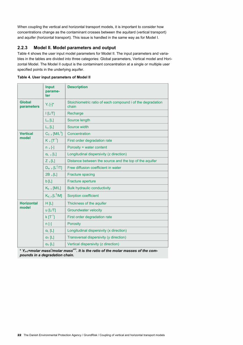
2.2.3 Model II. Model parameters and output
Table 4 shows the user input model parameters for Model II. The input parameters and varia-
bles in the tables are divided into three categories: Global parameters, Vertical model and Hori-
zontal Model. The Model II output is the contaminant concentration at a single or multiple user
specified points in the underlying aquifer.
Table 4. User input parameters of Model II
Input parame-ter
Description
Global parameters
Yi [-]* Stoichiometric ratio of each compound i of the degradation chain
I [L/T] Recharge
Lx [L] Source length
Ly [L] Source width
Vertical model
C0_v [M/L3] Concentration
K_v [T-1
] First order degradation rate
n_v [-] Porosity = water content
αL_v [L] Longitudinal dispersivity (z direction)
Z_v [L] Distance between the source and the top of the aquifer
Dw_v [L2/T]
Free diffusion coefficient in water
2B_v [L] Fracture spacing
b [L] Fracture aperture
Kb_v [M/L] Bulk hydraulic conductivity
Kd_v [L3/M] Sorption coefficient
Horizontal model
H [L] Thickness of the aquifer
u [L/T] Groundwater velocity
k [T-1
] First order degradation rate
n [-] Porosity
αL [L] Longitudinal dispersivity (x direction)
αT [L] Transversal dispersivity (y direction)
αV [L] Vertical dispersivity (z direction)
* Yi+1=molar massi/molar mass
i+1. It is the ratio of the molar masses of the com-
pounds in a degradation chain.

The Danish Environmental Protection Agency / GrundRisk / Coupling of vertical and horizontal transport models 23
2.3 Model III. Unsaturated zone overlying an unconfined aquifer The conceptual model of Model III is shown in Figure 6. Model III simulates the water phase
concentrations in the unsaturated zone overlying an unconfined aquifer using a downward ver-
tical transport model and then the concentrations in the aquifer using a horizontal transport
model. The contaminant source is represented by the length Lx, the width Ly and the source
concentration C0. The source can be located below terrain and is located at a user specified
distance from the top of the aquifer. The vertical transport model of Model III simulates the
water phase concentrations from the contaminant source to the top of the aquifer using a 3D
steady-state analytical solution.
The vertical transport model simulates the concentration C1(x,y,Zv) at the top of the aquifer
which is then used as input to the horizontal model to simulate the concentrations in the aquifer.
The concentration C1(x,y,Zv) is integrated over the x and y area at the groundwater table level
(Zv) and multiplied by the recharge rate I to obtain the contaminant mass input for the horizontal
model. The horizontal model simulates the concentrations in the aquifer using a 3D steady-
state analytical solution including advection and dispersion in the aquifer. The horizontal model
is a modified version of the horizontal model shown in Miljøstyrelsen (2016b) to account for a
larger contaminant discharge area at the groundwater table. The following sections describe the
vertical component of Model III, the coupling between the vertical and the horizontal transport
models, the horizontal model and the model parameters.
Figure 6. (Left) Conceptual model III. Contaminant transport from a source located in the
unsaturated zone, downward to the top of the aquifer and then horizontal transport in the
aquifer. (Right) Concentration at the top of the aquifer in plan view as a function of x and
y (z_v=18 m); the black line shows the location of the contaminant source (from the Mw
Gjøes Vej model application).
2.3.1 Model III. Unsaturated zone vertical transport model with
infiltration
The vertical model of Model III simulates the downward vertical contaminant transport in the
water phase in the unsaturated zone when the recharge is greater than zero. Contaminants are
transported in both the air and water phases. Diffusion is considered in the air phase, but not
in the water phase because vapour phase diffusion is several orders of magnitude larger than
that occurring in the aqueous phase (approximately 104 times larger. See Schwarzenbach et
al., 1993). Advection is considered in the water phase due to water infiltration, but air phase
advection is typically small and so is neglected.

24 The Danish Environmental Protection Agency / GrundRisk / Coupling of vertical and horizontal transport models
Gas transport is a significant process in the unsaturated zone. Many studies have shown that
diffusion in the gas phase is a dominant transport process in the unsaturated zone, particularly
for volatile compounds (Christophersen et al., 2005). Both field data and model results show
that the risk of contamination of groundwater consisting of volatile compounds is limited in are-
as in contact with the atmosphere due to diffusive transport and loss to the atmosphere (Chris-
tophersen et al., 2005; Lahvis et al., 2004; Grathwohl et al., 2002; Lahvis et al., 2000).
By summing the transport equations for water and air and employing the phase partitioning
expression Ca=KH∙Cw, Equation 6 is obtained.
( )( )w H a w ww w a H w w w w
R K C CK C q C
t z
aD D
Cw CONCENTRATION IN THE WATER
R RETARDATION FACTOR
KH DIMENSIONLESS HENRY’S LAW CONSTANT
θw WATER CONTENT
θa AIR CONTENT
t TIME
qw DARCY’S FLUX
Dw HYDRODYNAMIC DISPERSION IN WATER
Da HYDRODYNAMIC DISPERSION IN AIR
FIRST ORDER DEGRADATION RATE IN THE WATER PHASE
Equation 6
The 3D steady-state solution of Model III is given by Equation 7
(Miljøstyrelsen, 2016a; Troldborg, 2009). This equation was obtained with boundary and initial
conditions describing a source of concentration perpendicular to the flow direction
(Cw(x,y,0,t)=C0 for -Lx/2<x<Lx/2 and -Lx/2<x<Lx/2; Cw(x,y,0,t)=C0 otherwise) and a zero concen-
tration initial condition Cw(z,y,z,0)=0.

The Danish Environmental Protection Agency / GrundRisk / Coupling of vertical and horizontal transport models 25
' ' '0
0
( , , , ) ( , ) ( , ) ( , )8
w z x y
CC z x y t f z f x f y d
where:
2 2' 3/2
'
'
( , ) exp exp '2 4 4
2 2( , )2 2
2 2( , )2 2
zz z zz
x x
x
x x
y y
y
y y
z vz v zf z
D D DD
L Lx x
f x erf erfD D
L Ly y
f y erf erfD D
w
Iv
' w a HR R K
''
w
R
1 bd
w
R K
1b s n
d oc ocK f K
* *
'
w T w w a a Hx y
v D D KD D
R
* *
'
w L w w a a Hz
v D D KD
R
2,5*
,a
a d aD Dn
* * 410w aD D

26 The Danish Environmental Protection Agency / GrundRisk / Coupling of vertical and horizontal transport models
Cw CONCENTRATION IN THE WATER PHASE
t TIME
C0 CONCENTRATION IN THE SOURCE
I RECHARGE
erf ERROR FUNCTION
LX LENGTH OF THE SOURCE
LY WIDTH OF THE SOURCE
n POROSITY
ρb BULK DENSITY
ρs DENSITY OF MINERAL PARTICLES (2650 kg/m3)
Z VERTICAL DISTANCE FROM THE SOURCE
KH DIMENSIONLESS HENRY’S LAW CONSTANT
θw WATER CONTENT
θa AIR CONTENT
v PORE WATER VELOCITY
Dd,a FREE DIFFUSION COEFFICIENT IN AIR
Da* EFFECTIVE DIFFUSION COEFFICIENT IN AIR
Dw* EFFECTIVE DIFFUSION COEFFICIENT IN WATER
αL LONGITUDINAL DISPERSIVITY IN THE WATER PHASE
αT TRANSVERSAL DISPERSIVITY IN THE WATER PHASE
foc FRACTION OF ORGANIC CARBON
Koc PARTITION COEFFICIENT WITH RESPECT TO ORGANIC MATTER
FIRST ORDER DEGRADATION RATE
Equation 7
2.3.2 Model III. Coupling between the horizontal and vertical model
The conceptual model describing the coupling between the vertical and the horizontal transport
models is shown in Figure 6.
The vertical transport model simulates steady-state spatially distributed concentration C1(x,y,Zv)
(Equation 7) at the top of the aquifer. The spatially distributed concentration at the top of the
aquifer C1(x,y,Zv) is integrated over x and y and multiplied by the recharge rate in order to ob-
tain the contaminant mass discharge input to the horizontal model.
The steady-state solution (Equation 8) for the horizontal transport model is that of Miljøstyrelsen
(2016b). Equation 8 is similar to the solution of Miljøstyrelsen (2016b) (that is used on Model I,
II and V) but with 2 changes: (1) the mass flux [M/L2/T] from a point source at the top of the
aquifer is now described by the function J(x’,y’); (2) the integrals are calculated from -∞ to +∞,
because the contaminated area above the top of the aquifer is now larger than the original
source area.
The integrals are solved numerically over a finite integration interval. The integration interval
was set from –10max(Lx,Ly) to 10max(Lx,Ly). The integration interval selected based on a differ-
ent scenarios applied to the case study of MW Gjøes Vej (see Section 3.3.6). This selected
integration interval is assumed to be ok for other cases. The integration interval was selected
large enough so that almost 100% of the contaminant flux to the aquifer was captured. The
selection was made after testing several integration intervals in different scenarios that included
also very diffusive compounds.

The Danish Environmental Protection Agency / GrundRisk / Coupling of vertical and horizontal transport models 27
2 ( ', ')
, , exp2 24 x xy z
u x xJ x yc x y z dx dy
D Dn D D
1( ', ') ( ', ', )vJ x y C x y Z I
1
22 4 xu D
2 22 2x x
y z
D Dx x y y z
D D
x LD u
y TD u
z VD u
C1 WATER PHASE CONCENTRATION AT THE TOP OF THE AQUIFER (OUTPUT OF THE
VERTICAL TRANSPORT MODEL)
z DEPTH BELOW THE TOP OF THE AQUIFER
ZV DISTANCE BETWEEN THE CONTAMINANT SOURCE AND THE TOP OF THE AQUIFER
I RECHARGE
n POROSITY
αT TRANSVERSAL DISPERSIVITY IN THE WATER PHASE
αL LONGITUDINAL DISPERSIVITY IN THE WATER PHASE
αV VERTICAL DISPERSIVITY IN THE WATER PHASE
DX DISPERSION COEFFICIENT IN THE X DIRECTION (LONGITUDINAL)
DY DISPERSION COEFFICIENT IN THE Y DIRECTION (TRANSVERSAL)
DZ DISPERSION COEFFICIENT IN THE Z DIRECTION (TRANSVERSAL)
λ FIRST ORDER DEGRADATION RATE
u GROUNDWATER VELOCITY IN THE X DIRECTION
Equation 8

28 The Danish Environmental Protection Agency / GrundRisk / Coupling of vertical and horizontal transport models
2.3.3 Model III. Model parameters and output
Table 5 shows the user input model parameters for Model III. The input parameters and varia-
bles in the tables are divided into three groups: Global parameters, Vertical model and Horizon-
tal Model. The Model III output is the contaminant concentration at a single or multiple user
specified points x, y, z.
Table 5. User input parameters of Model III
Input parameter
Description
Global parameters
Yi [-]* Stoichiometric ratio of each compound i of the degrada-tion chain
I [L/T] Recharge
Lx [L] Source length
Ly [L] Source width
Vertical model
C0_v [M/L3] Concentration
k_v [T-1
] First order degradation rate
n_v [-] Porosity = water content
θw_v [-] Water content
αL_v [L] Longitudinal dispersivity (z direction)
αT_v [L] Transversal dispersivity (z direction)
Z_v [L] Distance between the source and the top of the aquifer
Da_v [L2/T]
Free diffusion coefficient of air
KH [-] Dimensionless Henry’s law constant
foc_v [-] Fraction of organic carbon
Koc_v [-] Partition coefficient with respect to organic matter
Horizontal model
H [L] Thickness of the aquifer
u [L/T] Groundwater velocity
k [T-1
] First order degradation rate
n [-] Porosity
αL [L] Longitudinal dispersivity (x direction)
αT [L] Transversal dispersivity (y direction)
αV [L] Vertical dispersivity (z direction)
* Yi+1=molar massi/molar mass
i+1. It is the ratio of the molar masses of the com-
pounds in a degradation chain.
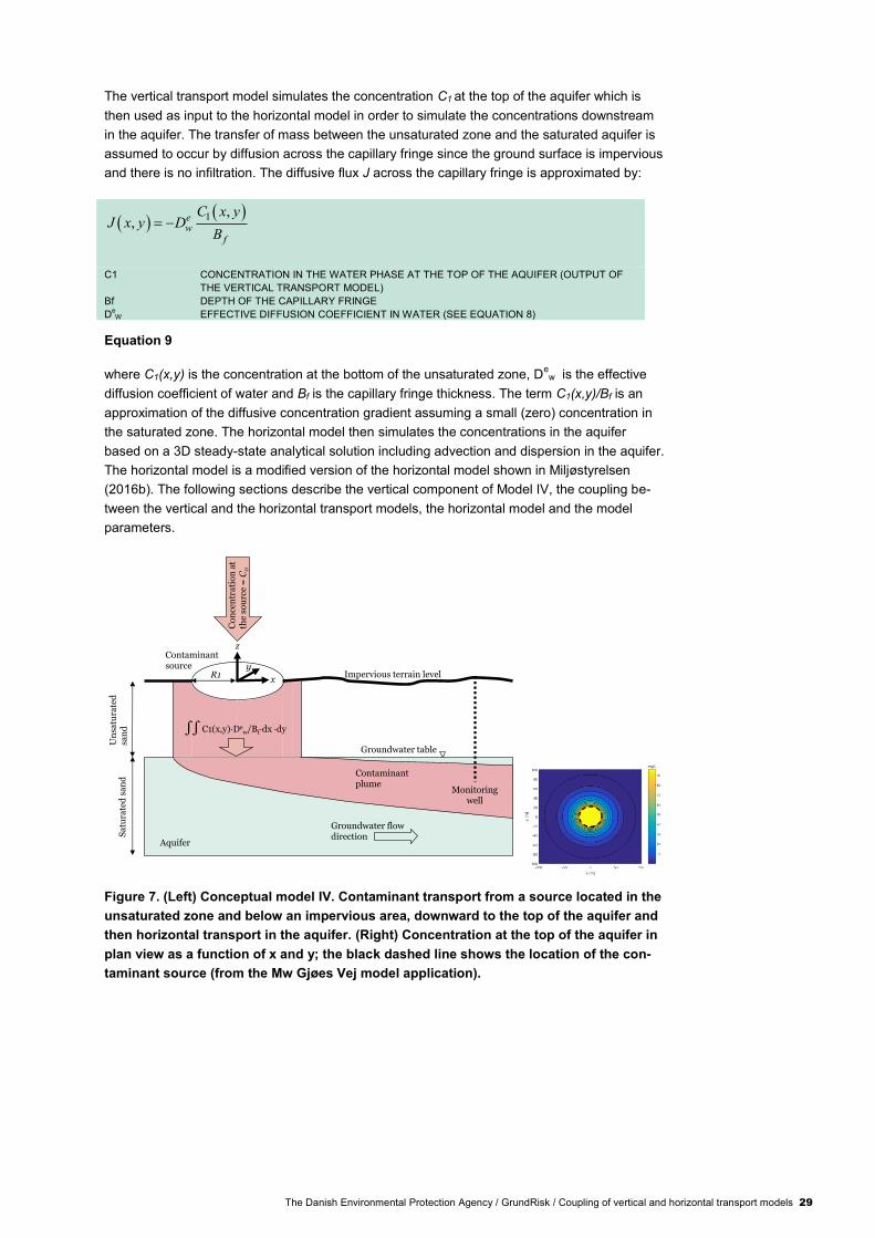
2.4 Model IV. Unsaturated zone under an impervious area with zero infiltration
The conceptual model for Model IV is shown in Figure 7. Model IV simulates the water phase
concentrations in the unsaturated zone overlying the unconfined aquifer with zero recharge
using a vertical transport model, and then the concentrations in the aquifer using a horizontal
transport model. The contaminant source is assumed to have a radius R1 and a source concen-
tration C0. The source can be located below the terrain. The vertical transport model of Model
IV simulates the water phase concentrations in the unsaturated zone between the contaminant
source and to the top of the aquifer using a 2D steady-state analytical solution. The steady-
state solution only considers 2D horizontal diffusive transport and thus concentration is not a
function of the distance between the contaminant source and the top of the aquifer (i.e. concen-
tration are constant in the vertical direction).
The Danish Environmental Protection Agency / GrundRisk / Coupling of vertical and horizontal transport models 29
The vertical transport model simulates the concentration C1 at the top of the aquifer which is
then used as input to the horizontal model in order to simulate the concentrations downstream
in the aquifer. The transfer of mass between the unsaturated zone and the saturated aquifer is
assumed to occur by diffusion across the capillary fringe since the ground surface is impervious
and there is no infiltration. The diffusive flux J across the capillary fringe is approximated by:
1 ,
, ew
f
C x yJ x y D
B
C1 CONCENTRATION IN THE WATER PHASE AT THE TOP OF THE AQUIFER (OUTPUT OF
THE VERTICAL TRANSPORT MODEL)
Bf DEPTH OF THE CAPILLARY FRINGE
DeW EFFECTIVE DIFFUSION COEFFICIENT IN WATER (SEE EQUATION 8)
Equation 9
where C1(x,y) is the concentration at the bottom of the unsaturated zone, De
w is the effective
diffusion coefficient of water and Bf is the capillary fringe thickness. The term C1(x,y)/Bf is an
approximation of the diffusive concentration gradient assuming a small (zero) concentration in
the saturated zone. The horizontal model then simulates the concentrations in the aquifer
based on a 3D steady-state analytical solution including advection and dispersion in the aquifer.
The horizontal model is a modified version of the horizontal model shown in Miljøstyrelsen
(2016b). The following sections describe the vertical component of Model IV, the coupling be-
tween the vertical and the horizontal transport models, the horizontal model and the model
parameters.
Figure 7. (Left) Conceptual model IV. Contaminant transport from a source located in the
unsaturated zone and below an impervious area, downward to the top of the aquifer and
then horizontal transport in the aquifer. (Right) Concentration at the top of the aquifer in
plan view as a function of x and y; the black dashed line shows the location of the con-
taminant source (from the Mw Gjøes Vej model application).
Groundwater table
Co
nce
ntr
ati
on
at
the
sou
rce
= C0
Impervious terrain levelR1x
y
z
Contaminantplume
Contaminantsource
Aquifer
Monitoringwell
∫∫ C1(x,y)∙Dew/Bf∙dx ∙dy
Un
satu
rate
d
san
dS
atu
rate
dsa
nd
Groundwater flow direction

30 The Danish Environmental Protection Agency / GrundRisk / Coupling of vertical and horizontal transport models
2.4.1 Model IV. Unsaturated zone vertical transport model without
infiltration
The vertical component of Model IV simulates the vertical contaminant transport in the water
phase in the unsaturated zone when there is zero recharge, i.e. in the presence of an impervi-
ous area such as thick clays or paved areas. In this case the main mechanism of contaminant
transport is gaseous diffusion in the horizontal direction.
Equation 10 the transport equation for volatile, reactive contaminants formulated in radial coor-
dinates and in the case of zero recharge.
2
2
( ) 1( )e ew H a w w wa H a w w w w
R K C C CK D D C
t r rr
Cw CONCENTRATION IN THE WATER PHASE
r RADIAL DISTANCE FROM THE CENTER OF THE CONTAMINANT SOURCE
R RETARDATION FACTOR
KH DIMENSIONLESS HENRY’S LAW CONSTANT
θw WATER CONTENT
θa AIR CONTENT
t TIME
Dea EFFECTIVE DIFFUSION COEFFICIENT IN AIR (SEE EQUATION 8)
Dew EFFECTIVE DIFFUSION COEFFICIENT IN WATER (SEE EQUATION 8)
FIRST ORDER DEGRADATION RATE
Equation 10
With the boundary conditions Cw(0<r<R1)=C0 and Cw(r→∞)=0, the steady-state solution was
given by (Spiegel, 1968; Miljøstyrelsen, 2016a) and shown in Equation 11. Equation 11 is im-
plemented in Model IV and it shows that the concentrations at steady-state are a function of the
radial distance (and not the vertical distance in the z direction).
00
0 1
( ) ( )( )
w
CC r K r
K R
w
e ea H a w wK D D
Cw CONCENTRATION IN THE WATER PHASE
K0() MODIFIED BESSEL FUNCTION OF SECOND KIND AND ORDER 0
KH DIMENSIONLESS HENRY’S LAW CONSTANT
C0 SOURCE CONCENTRATION
R RADIAL DISTANCE FROM THE CENTER OF THE CONTAMINANT SOURCE
R1 RADIUS OF THE CONTAMINANT SOURCE
θw WATER CONTENT
θa AIR CONTENT
Dea EFFECTIVE DIFFUSION COEFFICIENT IN AIR (SEE EQUATION 8)
Dew EFFECTIVE DIFFUSION COEFFICIENT IN WATER (SEE EQUATION 8)
FIRST ORDER DEGRADATION RATE
Equation 11
2.4.2 Model IV. Coupling between the horizontal and vertical model
The conceptual model describing the coupling between the vertical and the horizontal transport
model is shown in Figure 7. The vertical transport model simulates steady-state concentration
C1(x,y) (Equation 11) at the top of the aquifer. The concentration at the top of the aquifer C1(x,y)
is integrated over x and y and multiplied by the effective diffusion coefficient of water De
w and
divided by the capillary fringe in Bf order to obtain the contaminant flux.

The Danish Environmental Protection Agency / GrundRisk / Coupling of vertical and horizontal transport models 31
The steady-state solution (Equation 12) for the horizontal transport model is derived from
Miljøstyrelsen, 2016b. Equation 12 is similar to the solution of Miljøstyrelsen (2016b) but with 2
changes (similar to Model III): (1) the mass discharge [M/L2/T] from a point source at the top of
the aquifer is now described by the function J(x’,y’); (2) the integrals are calculated from -∞ to
+∞ because the contaminated area at the top of the aquifer is now larger than the original
source area.
The integrals are calculated numerically over a finite integration interval. The integration interval
are set from –150R1 +to 150R1. The integration interval selected based on a different scenari-
os applied to the case study of MW Gjøes Vej (see Section 3.4.1). This selected integration
interval is assumed to be appropriate for other cases.
( )
, , exp2 24
ox xy z
u x xJ rc x y z c dx dy
D Dn D D
( )( )
ew w
f
C r DJ r
B
2 2' 'r x y
1
22 4 xu D
2 22 2x x
y z
D Dx x y y z
D D
x LD u
y TD u
z VD u
Cw WATER PHASE CONCENTRATION CALCULATED USING EQUATION 11
Co BACKGROUND CONCENTRATION
Bf DEPTH OF THE CAPILLARY FRINGE
I RECHARGE
n POROSITY
Dx DISPERSION COEFFICIENT IN THE X DIRECTION (LONGITUDINAL)
Dy DISPERSION COEFFICIENT IN THE Y DIRECTION (TRANSVERSAL)
Dz DISPERSION COEFFICIENT IN THE Z DIRECTION (TRANSVERSAL)
αT TRANSVERSAL DISPERSIVITY IN THE WATER PHASE
αL LONGITUDINAL DISPERSIVITY IN THE WATER PHASE
αT TRANSVERSAL DISPERSIVITY IN THE WATER PHASE
λ FIRST ORDER DEGRADATION RATE
u GROUNDWATER VELOCITY IN THE X DIRECTION
Equation 12
2.4.3 Model IV. Model parameters and output
Table 6 shows the user input model parameters for Model IV. The input parameters and varia-
bles in the tables are divided into three categories: Global parameters, Vertical model and Hori-
zontal Model. The Model IV output is the contaminant concentration at a single or multiple user
specified points x, y, z.
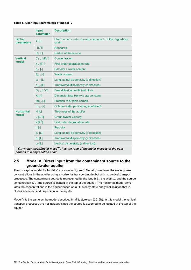
32 The Danish Environmental Protection Agency / GrundRisk / Coupling of vertical and horizontal transport models
Table 6. User input parameters of model IV
Input parameter
Description
Global parameters
Yi [-] Stoichiometric ratio of each compound i of the degradation chain
I [L/T] Recharge
R1 [L] Radius of the source
Vertical model
C0_v [M/L3] Concentration
k_v [T-1
] First order degradation rate
n_v [-] Porosity = water content
θw_v [-] Water content
αL_v [L] Longitudinal dispersivity (z direction)
αT_v [L] Transversal dispersivity (z direction)
Da_v [L2/T]
Free diffusion coefficient of air
KH [-] Dimensionless Henry’s law constant
foc_v [-] Fraction of organic carbon
Koc_v [-] Octanol-water partitioning coefficient
Horizontal model
H [L] Thickness of the aquifer
u [L/T] Groundwater velocity
k [T-1
] First order degradation rate
n [-] Porosity
αL [L] Longitudinal dispersivity (x direction)
αT [L] Transversal dispersivity (y direction)
αV [L] Vertical dispersivity (z direction)
* Yi+1=molar massi/molar mass
i+1. It is the ratio of the molar masses of the com-
pounds in a degradation chain.
2.5 Model V. Direct input from the contaminant source to the groundwater aquifer
The conceptual model for Model V is shown in Figure 8. Model V simulates the water phase
concentrations in the aquifer using a horizontal transport model but with no vertical transport
processes. The contaminant source is represented by the length Lx, the width Ly and the source
concentration C0. The source is located at the top of the aquifer. The horizontal model simu-
lates the concentrations in the aquifer based on a 3D steady-state analytical solution that in-
cludes advection and dispersion in the aquifer.
Model V is the same as the model described in Miljøstyrelsen (2016b). In this model the vertical
transport processes are not included since the source is assumed to be located at the top of the
aquifer.

The Danish Environmental Protection Agency / GrundRisk / Coupling of vertical and horizontal transport models 33
Figure 8. Conceptual model V. Horizontal contaminant transport from a source, located
at the top of the aquifer. (this models is the same as Miljøstyrelsen, 2016B).
2.6 Incorporation of reactive decay chains Reactive processes can be included in all five models in a similar way. In this section we only
report the equations used in the model, however Miljøstyrelsen (2016b) provides the details of
the approach.
Contaminant transport with reactive decay chains is described by Equation 13. In Equation 13,
R and D have the same value for all the components i.
1 1
1
2,3,...,
ii i i
i íi
i i i i i
cR c D c X ct
k c iX c
y k c k c i n
R RETARDATION FACTOR
Ci CONCENTRATION OF THE ITH COMPOUND
t TIME
D HYDRODYNAMIC DISPERSION COEFFICIENT IN WATER
ki FIRST ORDER DEGRADATION RATE OF THE ITH COMPOUND
yi STOICHIOMETRIC RATIO OF THE ITH COMPOUND
Equation 13
We employ the method of Sun et al. (1999a; 1999b). That is, we define a set of auxiliary con-
centration variables:
111
1
1
2,3,....,
i
iii l l
i jl ij l j
c i
a y kc c i n
k k
The contaminant transport Equation 13 is then solved by the methods described for each of the
models I-V with ia replacing ic . The solution for the components ic is then obtained from ia
using:
111
1
1
2,3,....,
i
iii l l
i jl ij l j
a i
c y ka c i n
k k

34 The Danish Environmental Protection Agency / GrundRisk / Coupling of vertical and horizontal transport models
3. Model applications
In this chapter several examples are presented showing how the models perform when applied
to contaminated sites in Denmark. Each example includes a brief description of a contaminated
site, shows how the model parameters were selected and presents the results. The modeling of
the contaminant transport at the contaminated sites is based on historical data, so the observed
contamination in the aquifer can be very different because the case may not consider results of
recent investigations and remedial actions. Comparison of the model results with observation
data was beyond the scope of this project. Note also that several simplifying assumptions are
made in each case so that they can be described by the model.
The computational time depends on the model. Model I, II, and V have computational time of
approximately 0-2 seconds for each simulated compound at a single point in the aquifer. Model
III and IV have computational time up to 5 minutes for each simulated compound at a single
point in the aquifer (this is because the numerical iterative convergence of the double integrals
of Model III and IV is computationally demanding). This means that if we need to extract a con-
centration profile in the aquifer with 10 points, Model III and IV can take up to 50 minutes for
each simulated compound. It may be possible to improve the computational time of Model III
and IV by optimizing the integration routines (used to solve the integrals of Equation 8 and 12)
and by exploiting geometrical symmetries of the model, however this was not attempted.
3.1 Rugårdsvej. Application of Model I Rugårdsvej in Odense is contaminated with DCE and VC. Machinery was manufactured at the
site in the period 1951-1989. Part of the area is now covered with asphalt. The source area is
about 30 m long and 10 m wide. The contaminant mass discharging through the source (as-
suming 300 mm/y infiltration according to JAGG 2.0) is 33 kg/y of DCE and 0.63 kg/y of VC. In
the simulation degradation of both components is assumed to occur.
3.1.1 Geology and hydrogeology
The primary aquifer is comprised of meltwater sand and gravel and is overlain by a 25-30 m
clay till. Locally there is a 1 m thick upper aquifer of fine-medium graded meltwater sand. The
secondary aquifer is about 12 m.b.s. and is overlain by fill and clay till with sand, silt and clay
lenses. Figure 9 shows the geological profile in the area of Rugårdsvej.
The water table in the secondary aquifer is located about 3-4 m.b.s. The clay layers are as-
sumed not to be fractured. JAGG 2.0 provides a recharge of 300 mm/y; Jørgensen et al.
(2007b) proposed a recharge of 100 mm/y and Miljøstyrelsen (2011) reported a recharge of 8
mm/y at the site.

The Danish Environmental Protection Agency / GrundRisk / Coupling of vertical and horizontal transport models 35
Figure 9. (A) Geological profile at Rugårdsvej 234-238 i Odense; (B) Plan view of the site
(Scheutz et al., 2008).
3.1.2 Contamination at the site
At Rugårdsvej 95% of the overall contaminant load from the source consists of DCE (Jørgen-
sen et al., 2007a). The original contaminant spill was TCE; however it has degraded into DCE
and VC which were found to be the main contaminants at the site.
The vertical and horizontal spreading of contaminants is shown in Figure 10. The source is
estimated to be 4-9 m.b.s. and the total concentration of chlorinated solvent in the source is
approximately 10 mg/kg of dry soil (Jørgensen et al. 2007a).
The highest concentration of DCE in the source zone is 371 mg/l (77 mg/kg of dry soil), and 7
mg/l VC (1.9 mg/kg of dry soil) was measured at the borehole M1 (Figure 9) at 4-5 m.b.s.
(Jørgensen et al. 2007). There are iron reducing conditions in and around the contaminant
source, with a trend to less reduced conditions with increasing distance from the source
(Jørgensen et al., 2007a).
Figure 10. Cross Section of the contaminant plume at Rugårdsvej (Jørgensen et al.,
2003).
3.1.3 Conceptual model and parameters for Rugårdsvej
Model I was chosen because the vertical transport processes from the source to the top of the
sand aquifer (Figure 9 and 10) take place in the saturated homogenous clay. The vertical con-
taminant transport of DCE and VC was simulated from the point where the highest concentra-
tions were measured to the top of the upper aquifer (the vertical distance between the source
and the upper aquifer was estimated to be approximately 6 m). The source concentrations of
DCE and VC are assumed to be equal to the highest measured concentrations to ensure a
conservative risk estimate in line with the recommendations in JAGG. The length and width of
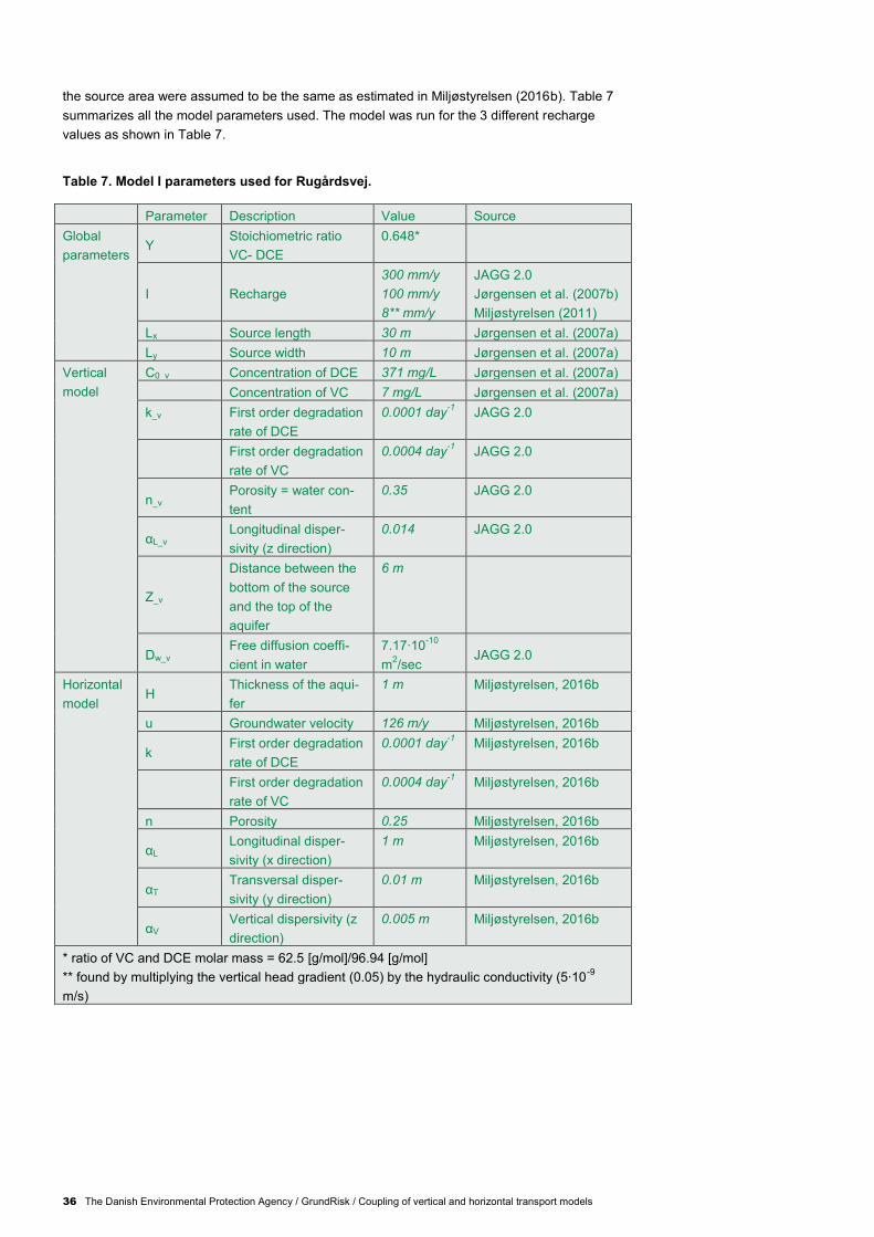
36 The Danish Environmental Protection Agency / GrundRisk / Coupling of vertical and horizontal transport models
the source area were assumed to be the same as estimated in Miljøstyrelsen (2016b). Table 7
summarizes all the model parameters used. The model was run for the 3 different recharge
values as shown in Table 7.
Table 7. Model I parameters used for Rugårdsvej.
Parameter Description Value Source
Global
parameters Y
Stoichiometric ratio
VC- DCE
0.648*
I Recharge
300 mm/y
100 mm/y
8** mm/y
JAGG 2.0
Jørgensen et al. (2007b)
Miljøstyrelsen (2011)
Lx Source length 30 m Jørgensen et al. (2007a)
Ly Source width 10 m Jørgensen et al. (2007a)
Vertical
model
C0_v Concentration of DCE 371 mg/L Jørgensen et al. (2007a)
Concentration of VC 7 mg/L Jørgensen et al. (2007a)
k_v First order degradation
rate of DCE
0.0001 day-1
JAGG 2.0
First order degradation
rate of VC
0.0004 day-1
JAGG 2.0
n_v Porosity = water con-
tent
0.35 JAGG 2.0
αL_v Longitudinal disper-
sivity (z direction)
0.014 JAGG 2.0
Z_v
Distance between the
bottom of the source
and the top of the
aquifer
6 m
Dw_v Free diffusion coeffi-
cient in water
7.17∙10-10
m2/sec
JAGG 2.0
Horizontal
model H
Thickness of the aqui-
fer
1 m Miljøstyrelsen, 2016b
u Groundwater velocity 126 m/y Miljøstyrelsen, 2016b
k First order degradation
rate of DCE
0.0001 day-1
Miljøstyrelsen, 2016b
First order degradation
rate of VC
0.0004 day-1
Miljøstyrelsen, 2016b
n Porosity 0.25 Miljøstyrelsen, 2016b
αL Longitudinal disper-
sivity (x direction)
1 m Miljøstyrelsen, 2016b
αT Transversal disper-
sivity (y direction)
0.01 m Miljøstyrelsen, 2016b
αV Vertical dispersivity (z
direction)
0.005 m Miljøstyrelsen, 2016b
* ratio of VC and DCE molar mass = 62.5 [g/mol]/96.94 [g/mol]
** found by multiplying the vertical head gradient (0.05) by the hydraulic conductivity (5∙10-9
m/s)
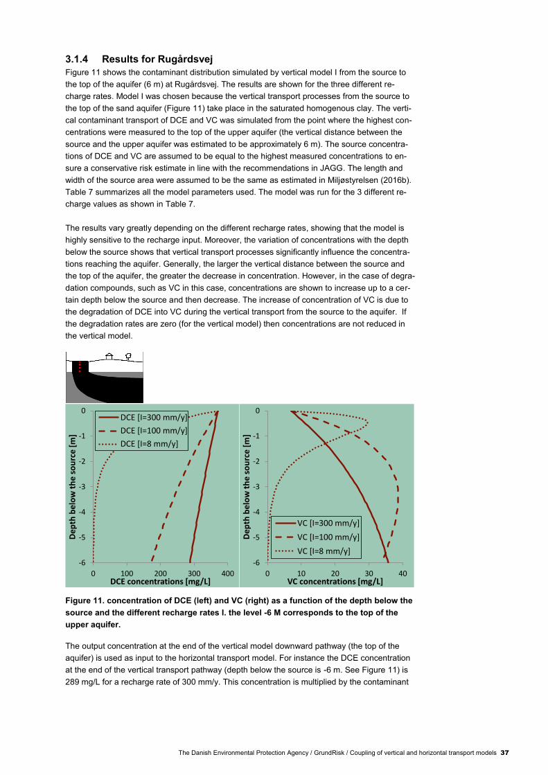
The Danish Environmental Protection Agency / GrundRisk / Coupling of vertical and horizontal transport models 37
3.1.4 Results for Rugårdsvej
Figure 11 shows the contaminant distribution simulated by vertical model I from the source to
the top of the aquifer (6 m) at Rugårdsvej. The results are shown for the three different re-
charge rates. Model I was chosen because the vertical transport processes from the source to
the top of the sand aquifer (Figure 11) take place in the saturated homogenous clay. The verti-
cal contaminant transport of DCE and VC was simulated from the point where the highest con-
centrations were measured to the top of the upper aquifer (the vertical distance between the
source and the upper aquifer was estimated to be approximately 6 m). The source concentra-
tions of DCE and VC are assumed to be equal to the highest measured concentrations to en-
sure a conservative risk estimate in line with the recommendations in JAGG. The length and
width of the source area were assumed to be the same as estimated in Miljøstyrelsen (2016b).
Table 7 summarizes all the model parameters used. The model was run for the 3 different re-
charge values as shown in Table 7.
The results vary greatly depending on the different recharge rates, showing that the model is
highly sensitive to the recharge input. Moreover, the variation of concentrations with the depth
below the source shows that vertical transport processes significantly influence the concentra-
tions reaching the aquifer. Generally, the larger the vertical distance between the source and
the top of the aquifer, the greater the decrease in concentration. However, in the case of degra-
dation compounds, such as VC in this case, concentrations are shown to increase up to a cer-
tain depth below the source and then decrease. The increase of concentration of VC is due to
the degradation of DCE into VC during the vertical transport from the source to the aquifer. If
the degradation rates are zero (for the vertical model) then concentrations are not reduced in
the vertical model.
Figure 11. concentration of DCE (left) and VC (right) as a function of the depth below the
source and the different recharge rates I. the level -6 M corresponds to the top of the
upper aquifer.
The output concentration at the end of the vertical model downward pathway (the top of the
aquifer) is used as input to the horizontal transport model. For instance the DCE concentration
at the end of the vertical transport pathway (depth below the source is -6 m. See Figure 11) is
289 mg/L for a recharge rate of 300 mm/y. This concentration is multiplied by the contaminant
-6
-5
-4
-3
-2
-1
0
0 100 200 300 400
De
pth
be
low
th
e s
ou
rce
[m
]
DCE concentrations [mg/L]
DCE [I=300 mm/y]
DCE [I=100 mm/y]
DCE [I=8 mm/y]
-6
-5
-4
-3
-2
-1
0
0 10 20 30 40
De
pth
be
low
th
e s
ou
rce
[m
]
VC concentrations [mg/L]
VC [I=300 mm/y]
VC [I=100 mm/y]
VC [I=8 mm/y]

38 The Danish Environmental Protection Agency / GrundRisk / Coupling of vertical and horizontal transport models
source area Lx·Ly and the recharge I rate in order to obtain the input mass discharge for the
horizontal model.
Figure 12 shows the concentrations of DCE and VC as a function of distance x in the aquifer
(y=0) up to 100 m downstream of the source. Two solutions are presented, the first one uses
Model I and the second one uses Model I excluding the vertical transport model (this means
that the input source concentrations of DCE and VC are directly applied to the horizontal model,
i.e. Model V is used). The concentrations do not vary in the z direction since the top of the aqui-
fer is thin and so the 2D horizontal transport model (Miljøstyrelsen, 2016b) was used. The re-
sults show that including the vertical transport model reduces the output concentrations of DCE
and increases the output concentration of VC. This is because DCE degrades to VC during the
vertical transport from the source to the top of the aquifer. A significant difference in concentra-
tions 100 m downstream of the source (particularly the VC concentration) is observed if the
vertical transport processes are included.
Figure 12. concentration of DCE (left) and VC (right) in the aquifer (note that there are
fully mixed conditions in the thin aquifer so there is no variation in concentrations in the
z direction). I=300 MM/Y.
3.1.5 Rugårdsvej example assuming contamination of benzene and
toluene
This section shows the results of a hypothetical example applying Model I to a site similar to
Rugårdsvej, but with the chlorinated solvents replaced by the more degradable compounds
benzene and toluene. Results demonstrate how changes in degradation rates change contami-
nant concentrations entering the aquifer.
The input model parameters are still as shown in Table 7 but with the following few changes
applied: (1) the input concentration of benzene and toluene are assumed to be C0_v=50 mg/l;
(2) the free diffusion coefficient in water of benzene is Dw_v=9.3∙10-10
m2/s and that of toluene is
Dw_v=8.56∙10-10
m2/s (JAGG 2.0); (3) the first order degradation rate of benzene is k_v=0.001
day-1
and for toluene is k_v=0.01 day-1
(JAGG 2.0), so about 10-100 times higher than for DCE
and VC.
0
20
40
60
80
100
120
0 25 50 75 100 125
con
cen
trat
ion
of
DC
E [m
g/L]
x-axis along the aquifer [m]
Model I withoutthe vertical model
Model I
Source
0
2
4
6
8
10
12
0 25 50 75 100 125
con
cen
trat
ion
of
VC
[m
g/L
]
x-axis along the aquifer [m]

The Danish Environmental Protection Agency / GrundRisk / Coupling of vertical and horizontal transport models 39
Figure 13 shows the results of the vertical transport model from the source to the top of the
aquifer (6 m.b.s.) using Model I. The results show a significant reduction of concentration with
increasing the depth below the source, particularly for toluene. The overall reduction of concen-
tration is more pronounced compared to the results shown above in Figure 13 for DCE. This is
because the first order degradation rates of toluene and benzene are much higher than DCE.
Figure 13. Model I application to high degradable compounds. concentration of benzene
and toluene as a function of the depth below the source. An infiltration rate of 300 MM/Y
was used and the level -6 M corresponds to the top of the aquifer.
Figure 14 shows the concentrations of benzene and toluene as a function of distance x in the
aquifer (y=0) up to 100 m downstream the source. Two solutions are presented, the first one
uses Model I and the second one uses Model I without the vertical transport processes (this
means that the input source concentrations of benzene and toluene are directly applied to the
horizontal model). The concentrations do not change in the z direction since the 2D solution
(Miljøstyrelsen, 2016b) was used. The results show a significant reduction of concentration if
the vertical transport processes are included.
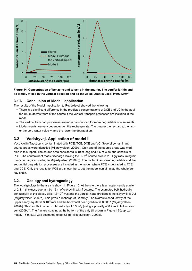
40 The Danish Environmental Protection Agency / GrundRisk / Coupling of vertical and horizontal transport models
Figure 14. Concentration of benzene and toluene in the aquifer. The aquifer is thin and
so is fully mixed in the vertical direction and so the 2d solution is used. I=300 MM/Y
3.1.6 Conclusion of Model I application
The results of the Model I application to Rugårdsvej showed the following:
There is a significant difference in the predicted concentrations of DCE and VC in the aqui-
fer 100 m downstream of the source if the vertical transport processes are included in the
model.
The vertical transport processes are more pronounced for more degradable contaminants.
Model results are very dependent on the recharge rate. The greater the recharge, the larg-
er the pore water velocity, and the lower the degradation.
3.2 Vadsbyvej. Application of model II Vasbyvej in Taastrup is contaminated with PCE, TCE, DCE and VC. Several contaminant
source areas were identified (Miljøstyrelsen, 2009b). Only one of the source areas was mod-
eled in this report. The source area considered is 10 m long and 5.5 m wide and consists of
PCE. The contaminant mass discharge leaving the 55 m2 source area is 2.6 kg/y (assuming 82
mm/y recharge according to Miljøstyrelsen (2009b)). The contaminants are degradable and the
sequential degradation processes are included in the model, where PCE is degraded to TCE
and DCE. Only the results for PCE are shown here, but the model can simulate the whole de-
cay chain.
3.2.1 Geology and hydrogeology
The local geology in the area is shown in Figure 15. At the site there is an upper sandy aquifer
of 2.4 m thickness overlain by 15 m of clayey till with fractures. The estimated bulk hydraulic
conductivity of the clayey till is 1.3∙10-8
m/s and the vertical head gradient in the clayey till is 0.2
(Miljøstyrelsen, 2009b). This gives a recharge of 82 mm/y. The hydraulic conductivity of the
upper sandy aquifer is 3∙10-5
m/s and the horizontal head gradient is 0.0007 (Miljøstyrelsen,
2009b). This results in a horizontal velocity of 3.3 m/y (using a porosity of 0.2 as in Miljøstyrel-
sen (2009b)). The fracture spacing at the bottom of the caly till shown in Figure 15 (approxi-
mately 15 m.b.s.) was estimated to be 5.6 m (Miljøstyrelsen, 2009b).
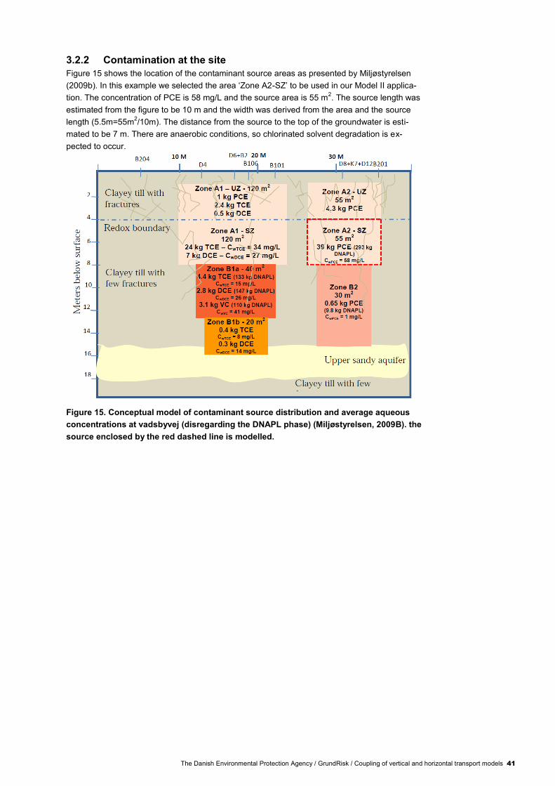
The Danish Environmental Protection Agency / GrundRisk / Coupling of vertical and horizontal transport models 41
3.2.2 Contamination at the site
Figure 15 shows the location of the contaminant source areas as presented by Miljøstyrelsen
(2009b). In this example we selected the area ‘Zone A2-SZ’ to be used in our Model II applica-
tion. The concentration of PCE is 58 mg/L and the source area is 55 m2. The source length was
estimated from the figure to be 10 m and the width was derived from the area and the source
length (5.5m=55m2/10m). The distance from the source to the top of the groundwater is esti-
mated to be 7 m. There are anaerobic conditions, so chlorinated solvent degradation is ex-
pected to occur.
Figure 15. Conceptual model of contaminant source distribution and average aqueous
concentrations at vadsbyvej (disregarding the DNAPL phase) (Miljøstyrelsen, 2009B). the
source enclosed by the red dashed line is modelled.

42 The Danish Environmental Protection Agency / GrundRisk / Coupling of vertical and horizontal transport models
3.2.3 Conceptual model and parameters for Vadsbyvej
Model II was chosen because the vertical transport processes from the source to the top of the
aquifer occur in a saturated fractured clay overlying the aquifer. Table 8 summarizes all the
model parameters used in Model II. The model was run for the 2 different recharge rates as
shown in Table 8.
Table 8. Model II parameters used for Vadsbyvej
Input
parameter
Description Value Source
Global
parameters I Recharge
250 mm/y
82 mm/y
JAGG 2.0
Miljøstyrelsen (2009b)
Lx Source length 10 m Estimated from Figure 15
Ly Source width 5.5 m Estimated from Figure 15
Vertical
model
C0_v Concentration of PCE 58 mg/L Miljøstyrelsen (2009b)
k_v First order degradation
rate of PCE
0.0005 day-1
JAGG 2.0
n_v Porosity = water con-
tent
0.3 Miljøstyrelsen (2009b)
αL_v Longitudinal disper-
sivity (z direction)
0.1 m Miljøstyrelsen (2009b)
Z_v
Distance between the
bottom of the source
and the top of the
aquifer
7 m Estimated from Figure 15
Dw_v Free diffusion coeffi-
cient in water PCE
5.71∙10-10
m2/sec
Miljøstyrelsen (2009b)
2B_v
Fracture spacing at the
bottom of the clay till 5.6 Miljøstyrelsen (2009b)
kb_v Bulk hydraulic conduc-
tivity
1.3∙10-8
m/sec Miljøstyrelsen (2009b)
Kd** Sorption coefficient 1.65 L/kg Lu et al. (2011)
Horizontal
model H
Thickness of the aqui-
fer
2.4 m Miljøstyrelsen (2009b)
u Groundwater velocity 3.3 m/y*
k First order degradation
rate of PCE
0.0005 day-1
JAGG 2.0
n Porosity 0.2 Miljøstyrelsen (2009b)
αL Longitudinal disper-
sivity (x direction)
1 m Miljøstyrelsen (2016b)
αT Transversal disper-
sivity (y direction)
0.01 m Miljøstyrelsen (2016b)
αV Vertical dispersivity (z
direction)
0.005 m Miljøstyrelsen (2016b)
* found by multiplying the horizontal head gradient (0.0007) with the hydraulic conductivity
(3∙10-5
m/s) and dividing by the porosity (0.2). Values obtained from Miljøstyrelsen (2009b).
** Kd values specific for clayey tills can be found in Lu et al. (2011)

The Danish Environmental Protection Agency / GrundRisk / Coupling of vertical and horizontal transport models 43
3.2.4 Results for Vadsbyvej
Figure 16 (left) shows the PCE concentration between the source and the top of the aquifer
(degradation of PCE to TCE and DCE was simulated, but only the results for PCE are shown).
Results for the two different recharge rates I of Table 8 are shown. Overall, the longer the per-
colation time from the source to the top of the aquifer, the greater the impact of degradation
during vertical transport and the higher the reduction in the concentrations reaching the aquifer.
The percolation time from the source to the top of the aquifer depends on the recharge I, frac-
ture spacing 2B, and bulk hydraulic conductivity Kb. When the degradation rates are zero (verti-
cal model) then the vertical model does not produce variations in the steady-state concentra-
tions. The reduction in concentration from the source to the top of the aquifer is approximately
25% when the recharge is I=82 mm/y, while it is only 8% when the recharge rate is 250 mm/yr.
One assumption made in all the models is that of steady-state. It is important to check the valid-
ity of this assumption. Figure 16 (right) shows the PCE concentration as a function of time simu-
lated using the model DTU v1D (Chambon et al., 2011). The results show that it takes approxi-
mately 20 years for a recharge of 250 mm/y, and 50 years for a recharge of 82 mm/y to reach
steady-state concentrations. The steady-state solution provides a conservative risk assessment
because transient concentrations are lower than those determined by the steady-state solution.
Since almost steady-state concentrations are obtained after 20 years it is acceptable to neglect
temporal changes in the concentration at the site.
Figure 16. Concentration of PCE as a function of the depth below the source and the
different recharge rates I. (left). the level -7 M corresponds to the top of the aquifer. Con-
centration of PCE as a function of time (using the model DTU v1d of Chambon et al.,
2011) at 7m depth (right).
The output concentration at the end of the vertical model downward pathway (the top of the
aquifer) is used as input to the horizontal transport model. For instance the PCE concentration
at the end of the vertical transport pathway (depth below the source -7 m. See Figure 16) is 53
mg/L for a recharge rate of 250 mm/y. This concentration is multiplied by the contaminant
source area Lx·Ly and the recharge I rate in order to obtain the input mass discharge for the
horizontal model.

44 The Danish Environmental Protection Agency / GrundRisk / Coupling of vertical and horizontal transport models
Figure 17 shows the concentrations of PCE as a function of distance x in the aquifer (y=0) up to
100 m downstream of the source. Two solutions are presented; the first one uses Model II and
the second one uses Model II without the vertical transport model (this means that the input
source concentrations of PCE are directly applied to the horizontal model, i.e. Model V). Be-
cause the aquifer is thin, the 2D horizontal model (Miljøstyrelsen, 2016b) was used and the
estimated concentrations in the aquifer do therefore not vary in the z direction. The results show
that including the vertical transport model reduces the output concentrations of PCE. However,
the difference in PCE concentration predicted by the two models at 100 m downstream of the
source is very small. This is because the groundwater velocity in the aquifer is very low (u=3.3
m/y) so that the residence time in the aquifer is very long, allowing for significant degradation to
occur before reaching a point 100 m downstream the source.
Figure 17. Concentration of PCE in the aquifer (there are fully mixed conditions in the
aquifer, a 2d solution is used so there is no variation in concentrations in the z direc-
tion). I=82 MM/Y. Note that concentrations along y-axis are log-scale.
3.2.5 The effect of the fracture spacing parameter 2B
The model input parameter fracture spacing 2B is difficult to estimate and Christiansen et al.
(2006), Videncenter for Jordforurening (2008), and Klint et al. (2013) showed that the fracture
spacing in Danish clayey tills can vary between 0 and 5 m in the top 8 m.b.s, and that the frac-
ture spacing increases with the depth below the surface. Figure 18 shows the PCE concentra-
tions from Model II as a function of the depth below the source and for different fracture spacing
2B (when the fracture spacing, recharge rates and bulk hydraulic conductivity are specified, the
model calculates the resulting vertical gradient and fracture aperture using Equation 5). The
results show that the smaller the fracture spacing, the higher the reduction in PCE concentra-
tions. This is because a smaller fracture spacing reduces the percolation time of contaminants
from the source to the top of the aquifer (the same amount of infiltration is spread over a larger
number of fractures that are now closer to each-other).

The Danish Environmental Protection Agency / GrundRisk / Coupling of vertical and horizontal transport models 45
Figure 18. Concentration as a function of the depth below the source and different frac-
ture spacing 2b. the recharge rate is I=250 MM/Y.
3.2.6 The assumption of fully mixed conditions at the bottom of the
fractured aquitard
The fracture transport Model II assumes that the contaminant output from the fractures is fully
mixed over the whole source area at the top of the aquifer. This section investigates the validity
of this assumption.
To test the fully mixed assumption, a coupled COMSOL Multiphysics model was used to run
various scenarios where the contaminant flux from the fractured clay is mixed at the top of the
aquifer in different ways. Each scenario simulates the contaminant concentration in the aquifer
based on different fracture distributions.
The scenarios are illustrated in Figure 19 and are:
1. Matlab, fully mixed. The concentrations in the aquifer are simulated using the horizon-
tal Model II. The contaminant mass discharge is uniform over the source area.
2. Multiphysics, fully mixed. The concentrations in the aquifer are simulated using Mul-
tiphysics with a uniform mass discharge over the source area.
3. Multiphysics, perpendicular fractures. The source is modelled with 2 line sources hav-
ing a specified contaminant flux per unit length and with a distance of 2B=5.6m. The
line source is perpendicular to the flow direction in the aquifer (aligned with the y axes
of Model II).
4. Multiphysics, angled fractures. The source is modelled as a line source having a speci-
fied contaminant flux per unit length. The line source is oriented with an angle of 30
degrees compared to the flow direction in the aquifer.
5. Multiphysics, longitudinal fracture. The source is modelled as a line source having a
specified contaminant flux per unit length. The line source is oriented in the flow direc-
tion in the aquifer (aligned with the x axes of Model II).
6. Multiphysics, longitudinal parallel fracture. The source is modelled as a line source
having a specified contaminant flux per unit length. The line source is oriented in the
flow direction in the aquifer (aligned with the x axes of Model II).
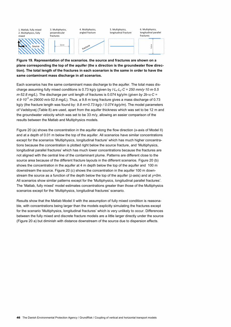
46 The Danish Environmental Protection Agency / GrundRisk / Coupling of vertical and horizontal transport models
Figure 19. Representation of the scenarios. the source and fractures are shown on a
plane corresponding the top of the aquifer (the x direction is the groundwater flow direc-
tion). The total length of the fractures in each scenarion is the same in order to have the
same contaminant mass discharge in all scenarios.
Each scenarios has the same contaminant mass discharge to the aquifer. The total mass dis-
charge assuming fully mixed conditions is 0.73 kg/y (given by I∙Lx∙Ly∙C = 250 mm/y∙10 m∙5.5
m∙52.8 mg/L). The discharge per unit length of fractures is 0.074 kg/y/m (given by 2b∙vf∙C =
4.9·10-5
m∙29000 m/s∙52.8 mg/L). Thus, a 9.8 m long fracture gives a mass discharge of 0.73
kg/y (the fracture length was found by: 9.8 m=0.73 kg/y / 0.074 kg/y/m). The model parameters
of Vadsbyvej (Table 8) are used, apart from the aquifer thickness which was set to be 12 m and
the groundwater velocity which was set to be 33 m/y, allowing an easier comparison of the
results between the Matlab and Multiphysics models.
Figure 20 (a) shows the concentration in the aquifer along the flow direction (x-axis of Model II)
and at a depth of 0.01 m below the top of the aquifer. All scenarios have similar concentrations
except for the scenarios ‘Multiphysics, longitudinal fracture’ which has much higher concentra-
tions because the concentration is plotted right below the source fracture, and ‘Multiphysics,
longitudinal parallel fractures’ which has much lower concentrations because the fractures are
not aligned with the central line of the contaminant plume. Patterns are different close to the
source area because of the different fracture layouts in the different scenarios. Figure 20 (b)
shows the concentration in the aquifer at 4 m depth below the top of the aquifer and 100 m
downstream the source. Figure 20 (c) shows the concentration in the aquifer 100 m down-
stream the source as a function of the depth below the top of the aquifer (z-axis) and at y=0m.
All scenarios show similar patterns except for the ‘Multiphysics, longitudinal parallel fractures’.
The ‘Matlab, fully mixed’ model estimates concentrations greater than those of the Multiphysics
scenarios except for the ‘Multiphysics, longitudinal fractures’ scenario.
Results show that the Matlab Model II with the assumption of fully mixed condition is reasona-
ble, with concentrations being larger than the models explicitly simulating the fractures except
for the scenario ‘Multiphysics, longitudinal fractures’ which is very unlikely to occur. Differences
between the fully mixed and discrete fracture models are a little larger directly under the source
(Figure 20 a) but diminish with distance downstream of the source due to dispersion effects.
1. Matlab, fully mixed2. Multiphysics, fully mixed
3. Multiphysics, perpendicular fractures
4. Multiphysics, angled fracture
5. Multiphysics, longitudinal fracture
uSource
6. Multiphysics, longitudinal parallel fractures
5.6 m
5.6
mx
y
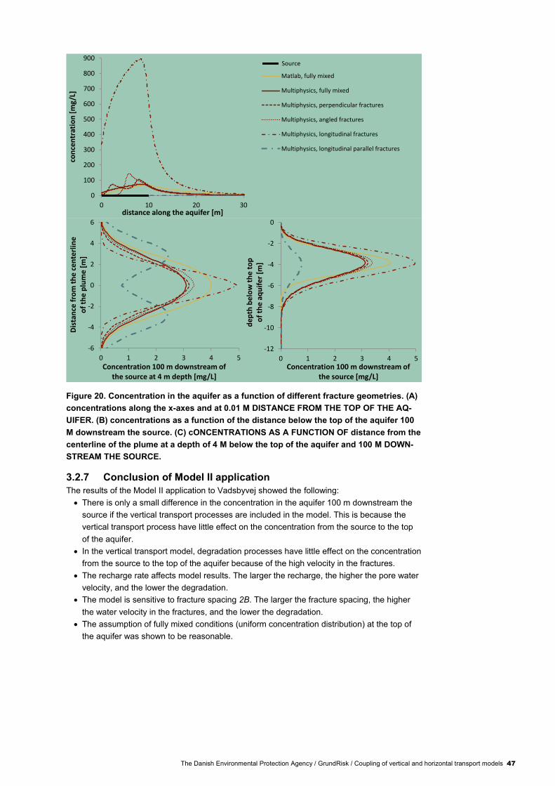
The Danish Environmental Protection Agency / GrundRisk / Coupling of vertical and horizontal transport models 47
Figure 20. Concentration in the aquifer as a function of different fracture geometries. (A)
concentrations along the x-axes and at 0.01 M DISTANCE FROM THE TOP OF THE AQ-
UIFER. (B) concentrations as a function of the distance below the top of the aquifer 100
M downstream the source. (C) cONCENTRATIONS AS A FUNCTION OF distance from the
centerline of the plume at a depth of 4 M below the top of the aquifer and 100 M DOWN-
STREAM THE SOURCE.
3.2.7 Conclusion of Model II application
The results of the Model II application to Vadsbyvej showed the following:
There is only a small difference in the concentration in the aquifer 100 m downstream the
source if the vertical transport processes are included in the model. This is because the
vertical transport process have little effect on the concentration from the source to the top
of the aquifer.
In the vertical transport model, degradation processes have little effect on the concentration
from the source to the top of the aquifer because of the high velocity in the fractures.
The recharge rate affects model results. The larger the recharge, the higher the pore water
velocity, and the lower the degradation.
The model is sensitive to fracture spacing 2B. The larger the fracture spacing, the higher
the water velocity in the fractures, and the lower the degradation.
The assumption of fully mixed conditions (uniform concentration distribution) at the top of
the aquifer was shown to be reasonable.
0
100
200
300
400
500
600
700
800
900
0 10 20 30
con
cen
trat
ion
[m
g/L]
distance along the aquifer [m]
Matlab, fully mixed
Multiphysics, fully mixed
Multiphysics, perpendicular fractures
Multiphysics, angled fractures
Multiphysics, longitudinal fractures
Multiphysics, longitudinal parallel fractures
Source
-6
-4
-2
0
2
4
6
0 1 2 3 4 5
Dis
tan
ce f
rom
th
e ce
nte
rlin
e o
f th
e p
lum
e [m
]
Concentration 100 m downstream of the source at 4 m depth [mg/L]
-12
-10
-8
-6
-4
-2
0
0 1 2 3 4 5
dep
th b
elo
w t
he
top
o
f th
e aq
uif
er [
m]
Concentration 100 m downstream of the source [mg/L]

48 The Danish Environmental Protection Agency / GrundRisk / Coupling of vertical and horizontal transport models
3.3 MW Gjøes Vej. Application of model III At MW Gjøes Vej 8 in Reerslev a former dry-cleaning facility, operating in the period 1956-
1977, has caused widespread contamination with PCE. It has been estimated that the amount
of PCE and degradation products spilled at the site is between 3 and 10 tons with PCE com-
prising about 50% of the total weight (Niras, 2009).
3.3.1 Geology and hydrogeology
The local geology is shown in Figure 21. The top 7 m consists of unsaturated clayey till and
then 20 m of meltwater sand and gravel. Only the lowest part of the sand is saturated. Below
the sand and gravel layer there is a 1 m thick layer of clayey till that extends approximately
1500 m downstream of the contaminant source. Below the clayey till there is a 25 m deep re-
gional limestone aquifer (Krüger, 2004).
The upper secondary aquifer is unconfined and the head level about 25 m.b.s. There is down-
ward vertical advective flow in the clayey till layer that is assumed to equal the recharge rate.
Figure 21. Geological and conceptual contaminant transport model at MW Gjøes Vej. The
red dotted line shows approximately the area that is modelled. Modified from niras
(2009).
3.3.2 Contamination at the site
There are two areas contaminated by chlorinated solvents exceeding the quality criteria of the
Danish EPA (5 mg/kg) (Krüger, 2004; Miljøstyrelsen, 2014). The concentration that are used as
input to Model III are greatest at 3.0-5.0 m.b.s. (Krüger, 2004). The areal extent of the contami-
nant source was assumed to be the same as that estimated in Miljøstyrelsen (2016b).
3.3.3 Conceptual model and parameters for MW Gløes Vej
Model III was selected because vertical transport from the source to the top of the aquifer oc-
curs in an unsaturated sand and the recharge in the area is greater than zero. The vertical
contaminant transport was simulated from the top of the sandy layer (assumed to be the bottom
of the source) to the groundwater table (the red dotted line of Figure 21 shows the model area).
The vertical distance between the bottom of the source zone (i.e. the the sand) and the top of
the unconfined aquifer was estimated by Miljøstyrelsen (2011) to be approximately 18 m. The
source concentrations are assumed to be equal to the highest measured concentrations. The
length and width of the source area were assumed to be the same as estimated in Miljøstyrel-
sen (2016b). The horizontal model simulates the transport only in the uppermost secondary
aquifer which is situated on top of a thin clayey till layer (27-29 m.b.s., Figure 21). Table 9
summarizes the model parameters used.
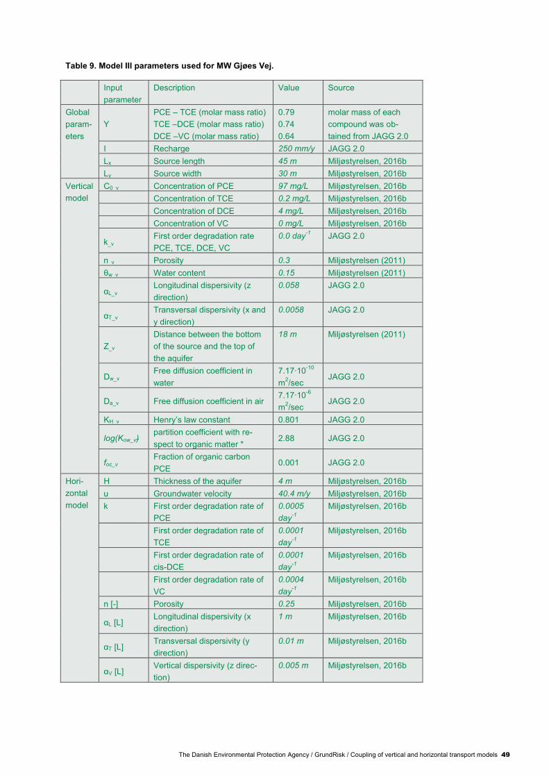
The Danish Environmental Protection Agency / GrundRisk / Coupling of vertical and horizontal transport models 49
Table 9. Model III parameters used for MW Gjøes Vej.
Input
parameter
Description Value Source
Global
param-
eters
Y
PCE – TCE (molar mass ratio)
TCE –DCE (molar mass ratio)
DCE –VC (molar mass ratio)
0.79
0.74
0.64
molar mass of each
compound was ob-
tained from JAGG 2.0
I Recharge 250 mm/y JAGG 2.0
Lx Source length 45 m Miljøstyrelsen, 2016b
Ly Source width 30 m Miljøstyrelsen, 2016b
Vertical
model
C0_v Concentration of PCE 97 mg/L Miljøstyrelsen, 2016b
Concentration of TCE 0.2 mg/L Miljøstyrelsen, 2016b
Concentration of DCE 4 mg/L Miljøstyrelsen, 2016b
Concentration of VC 0 mg/L Miljøstyrelsen, 2016b
k_v First order degradation rate
PCE, TCE, DCE, VC
0.0 day-1
JAGG 2.0
n_v Porosity 0.3 Miljøstyrelsen (2011)
θw_v Water content 0.15 Miljøstyrelsen (2011)
αL_v Longitudinal dispersivity (z
direction)
0.058 JAGG 2.0
αT_v Transversal dispersivity (x and
y direction)
0.0058 JAGG 2.0
Z_v
Distance between the bottom
of the source and the top of
the aquifer
18 m Miljøstyrelsen (2011)
Dw_v Free diffusion coefficient in
water
7.17∙10-10
m2/sec
JAGG 2.0
Da_v
Free diffusion coefficient in air 7.17∙10
-6
m2/sec
JAGG 2.0
KH_v Henry’s law constant 0.801 JAGG 2.0
log(Kow_v) partition coefficient with re-
spect to organic matter * 2.88 JAGG 2.0
foc_v Fraction of organic carbon
PCE 0.001 JAGG 2.0
Hori-
zontal
model
H Thickness of the aquifer 4 m Miljøstyrelsen, 2016b
u Groundwater velocity 40.4 m/y Miljøstyrelsen, 2016b
k
First order degradation rate of
PCE
0.0005
day-1
Miljøstyrelsen, 2016b
First order degradation rate of
TCE
0.0001
day-1
Miljøstyrelsen, 2016b
First order degradation rate of
cis-DCE
0.0001
day-1
Miljøstyrelsen, 2016b
First order degradation rate of
VC
0.0004
day-1
Miljøstyrelsen, 2016b
n [-] Porosity 0.25 Miljøstyrelsen, 2016b
αL [L] Longitudinal dispersivity (x
direction)
1 m Miljøstyrelsen, 2016b
αT [L] Transversal dispersivity (y
direction)
0.01 m Miljøstyrelsen, 2016b
αV [L] Vertical dispersivity (z direc-
tion)
0.005 m Miljøstyrelsen, 2016b

50 The Danish Environmental Protection Agency / GrundRisk / Coupling of vertical and horizontal transport models
3.3.4 Results for MW Gjøes Vej
Figure 22 shows the PCE concentration as a function of the depth below the source (left) and at
the top of the aquifer (right). Figure 22 shows that the contaminant spreads in the unsaturated
zone, leading to a decrease in concentrations at the top of the aquifer.
Figure 22. Concentration in a vertical cross section below the source (y=0 M) (left). Pce
concentration at the top of the aquifer in plan view (right) (z_v=18 M); the black line
shows the location of the contaminant source.
Figure 23 shows the concentration determined by the vertical transport model III in the unsatu-
rated zone from the source to the top of the aquifer (18 m.b.s.). The results show about small
reduction of concentration of all compounds with increasing depth below the source except for
VC which is constant and equal to zero. The concentrations at the top of the aquifer (at the
location x=0 m and y=0 m) are about 18% smaller than the source concentrations. The reduc-
tion in concentration is due to diffusion in the gas phase (degradation is not assumed to take
place because of aerobic conditions). The greater the diffusion in the gas phase is, the greater
the reduction in concentrations below the source will be (the contribution of the diffusion pro-
cess in the water phase is insignificant).
Figure 23. Concentration of PCE, TCE, cis-DCE and VC as a function of the depth below
the source simulated with Model III. the level -18 m corresponds to the top of the uncon-
fined aquifer.
-18
-16
-14
-12
-10
-8
-6
-4
-2
0
0 20 40 60 80 100
Dep
th b
elo
w t
he
sou
rce
[m
]
concentrations [mg/L]
PCE
-18
-16
-14
-12
-10
-8
-6
-4
-2
0
0 1 2 3 4
concentrations [mg/L]
TCEcis-DCEVC
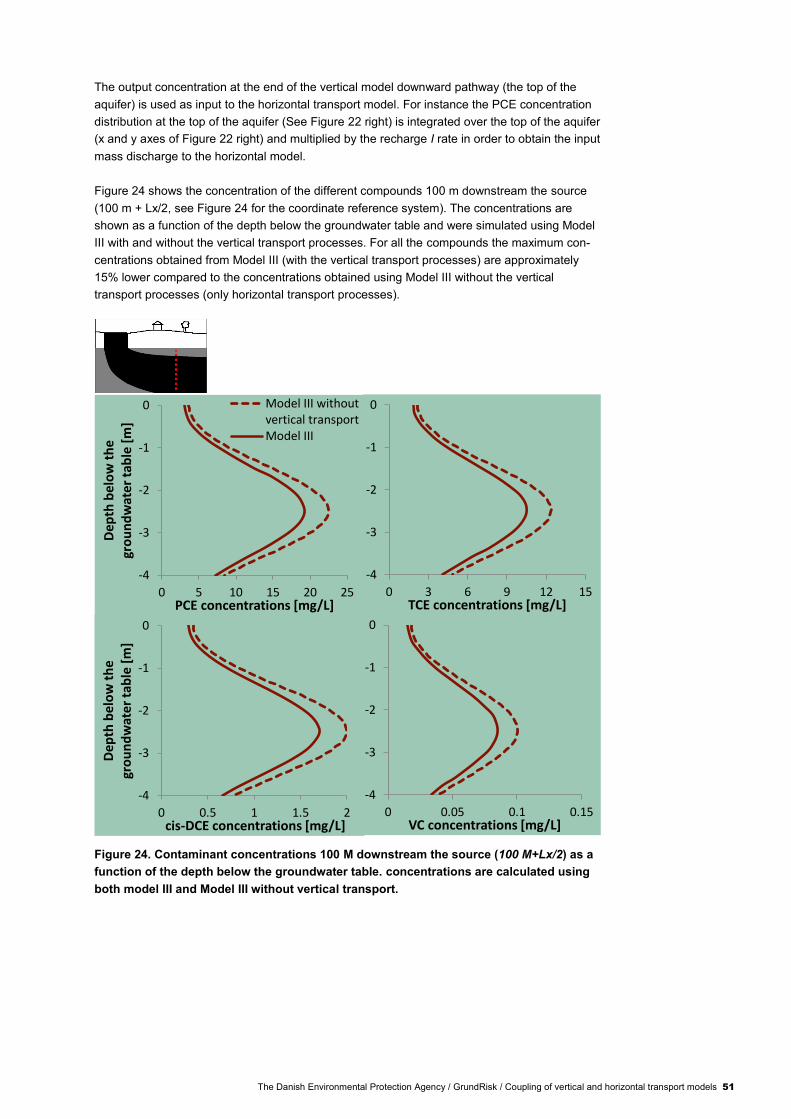
The Danish Environmental Protection Agency / GrundRisk / Coupling of vertical and horizontal transport models 51
The output concentration at the end of the vertical model downward pathway (the top of the
aquifer) is used as input to the horizontal transport model. For instance the PCE concentration
distribution at the top of the aquifer (See Figure 22 right) is integrated over the top of the aquifer
(x and y axes of Figure 22 right) and multiplied by the recharge I rate in order to obtain the input
mass discharge to the horizontal model.
Figure 24 shows the concentration of the different compounds 100 m downstream the source
(100 m + Lx/2, see Figure 24 for the coordinate reference system). The concentrations are
shown as a function of the depth below the groundwater table and were simulated using Model
III with and without the vertical transport processes. For all the compounds the maximum con-
centrations obtained from Model III (with the vertical transport processes) are approximately
15% lower compared to the concentrations obtained using Model III without the vertical
transport processes (only horizontal transport processes).
Figure 24. Contaminant concentrations 100 M downstream the source (100 M+Lx/2) as a
function of the depth below the groundwater table. concentrations are calculated using
both model III and Model III without vertical transport.
-4
-3
-2
-1
0
0 0.5 1 1.5 2
Dep
th b
elo
w t
he
gr
ou
nd
wat
er t
able
[m
]
cis-DCE concentrations [mg/L]
-4
-3
-2
-1
0
0 3 6 9 12 15TCE concentrations [mg/L]
-4
-3
-2
-1
0
0 5 10 15 20 25
Dep
th b
elo
w t
he
gr
ou
nd
wat
er t
able
[m
]
PCE concentrations [mg/L]
Model III withoutvertical transportModel III
-4
-3
-2
-1
0
0 0.05 0.1 0.15VC concentrations [mg/L]
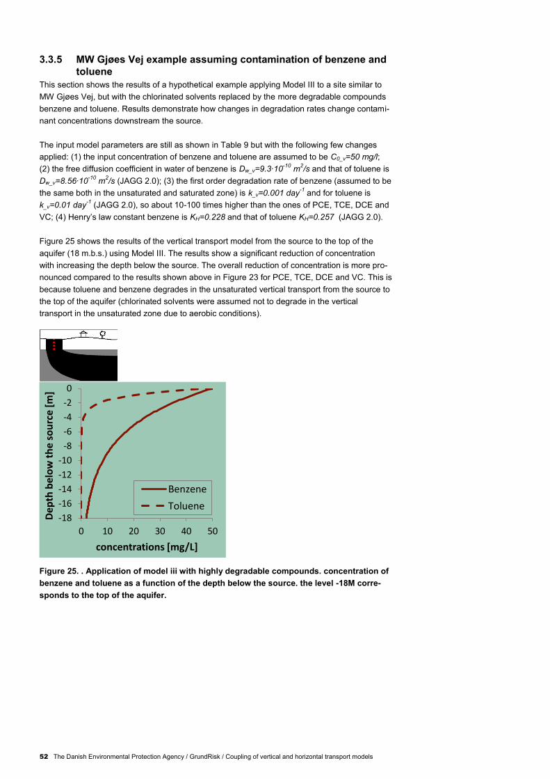
52 The Danish Environmental Protection Agency / GrundRisk / Coupling of vertical and horizontal transport models
3.3.5 MW Gjøes Vej example assuming contamination of benzene and
toluene
This section shows the results of a hypothetical example applying Model III to a site similar to
MW Gjøes Vej, but with the chlorinated solvents replaced by the more degradable compounds
benzene and toluene. Results demonstrate how changes in degradation rates change contami-
nant concentrations downstream the source.
The input model parameters are still as shown in Table 9 but with the following few changes
applied: (1) the input concentration of benzene and toluene are assumed to be C0_v=50 mg/l;
(2) the free diffusion coefficient in water of benzene is Dw_v=9.3∙10-10
m2/s and that of toluene is
Dw_v=8.56∙10-10
m2/s (JAGG 2.0); (3) the first order degradation rate of benzene (assumed to be
the same both in the unsaturated and saturated zone) is k_v=0.001 day-1
and for toluene is
k_v=0.01 day-1
(JAGG 2.0), so about 10-100 times higher than the ones of PCE, TCE, DCE and
VC; (4) Henry’s law constant benzene is KH=0.228 and that of toluene KH=0.257 (JAGG 2.0).
Figure 25 shows the results of the vertical transport model from the source to the top of the
aquifer (18 m.b.s.) using Model III. The results show a significant reduction of concentration
with increasing the depth below the source. The overall reduction of concentration is more pro-
nounced compared to the results shown above in Figure 23 for PCE, TCE, DCE and VC. This is
because toluene and benzene degrades in the unsaturated vertical transport from the source to
the top of the aquifer (chlorinated solvents were assumed not to degrade in the vertical
transport in the unsaturated zone due to aerobic conditions).
Figure 25. . Application of model iii with highly degradable compounds. concentration of
benzene and toluene as a function of the depth below the source. the level -18M corre-
sponds to the top of the aquifer.
-18
-16
-14
-12
-10
-8
-6
-4
-2
0
0 10 20 30 40 50
Dep
th b
elo
w t
he
sou
rce
[m
]
concentrations [mg/L]
Benzene
Toluene

The Danish Environmental Protection Agency / GrundRisk / Coupling of vertical and horizontal transport models 53
Figure 26 shows the concentrations of benzene and toluene as a function of distance x in the
aquifer (y=0) up to 100 m downstream the source. Two solutions are presented, the first one
uses Model III and the second one uses Model III without the vertical transport processes (this
means that the input source concentrations of benzene and toluene are directly applied to the
horizontal model). The results show a significant reduction of concentration if the vertical
transport processes are included.
Figure 26. Model III application to easy degradable compounds. concentrations of ben-
zene and toluene in the aquifer.
3.3.6 Determining the numerical integration intervals of Model III
In order to couple the vertical and the horizontal transport models in Model III and to determine
the resulting concentrations in the aquifer downstream of the source, it is necessary to compute
the integrals of Equation 8 numerically. Numerical integration from -∞ to +∞ is computationally
expensive, so to reduce computational time the integration interval was selected to be from -
10∙max(Lx,Ly) to +10∙max(Lx,Ly). In the following it is investigated how the results are influ-
enced by the selection of different finite integration intervals and whether the selected integra-
tion interval of [-10∙max(Lx,Ly); 10∙max(Lx,Ly)] is appropriate for this case and for other contam-
inated sites.
Figure 27 shows the PCE mass discharge at the top of the aquifer (y-axes) as a function of
different integration intervals (x-axes) and different air diffusion coefficients. These results were
produced using similar parameters to MW Gjøes Vej (Table 9). Different air diffusion coeffi-
cients Da_v (up to 7·10-4
m2/s) were used so that more volatile compounds could be included in
the analysis. Results show that as the air diffusion coefficient increases, the numerical integra-
tion interval required to accurately calculate the PCE mass discharge to the top of the aquifer
increases. This is because the larger the air diffusion coefficient, the greater the spreading of
contaminant in space. Figure 27 shows that the integration interval 10∙max(Lx,Ly) is large
enough to capture essentially all of the mass discharge at the top of the aquifer. This integration
interval is specific for this case. The integration intervals are expected to increase with increas-
ing air diffusion coefficient Da_v, the distance between the source and the top of the aquifer Z_v
and the extend of the contaminant source Lx, Ly. Nevertheless, the integration interval
10∙max(Lx,Ly) is assumed to be reasonable for other cases since this case included a high air
diffusion coefficient and the distance between the source and aquifer was large (18 m).
-4
-3
-2
-1
0
0 0.3 0.6 0.9 1.2Toluene concentration [ug/L]
-4
-3
-2
-1
0
0 1 2 3 4 5 6 7
Dep
th b
elo
w t
he
gr
ou
nd
wat
er t
able
[m
]
Benzene concentration [mg/L]
Model III withoutvertical model
Model III
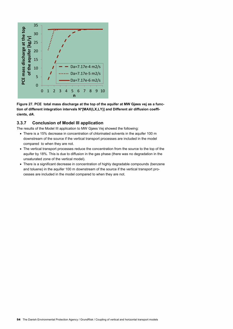
54 The Danish Environmental Protection Agency / GrundRisk / Coupling of vertical and horizontal transport models
Figure 27. PCE total mass discharge at the top of the aquifer at MW Gjøes vej as a func-
tion of different integration intervals N*[MAX(LX,LY)] and Different air diffusion coeffi-
cients, dA.
3.3.7 Conclusion of Model III application
The results of the Model III application to MW Gjøes Vej showed the following:
There is a 15% decrease in concentration of chlorinated solvents in the aquifer 100 m
downstream of the source if the vertical transport processes are included in the model
compared to when they are not.
The vertical transport processes reduce the concentration from the source to the top of the
aquifer by 18%. This is due to diffusion in the gas phase (there was no degradation in the
unsaturated zone of the vertical model).
There is a significant decrease in concentration of highly degradable compounds (benzene
and toluene) in the aquifer 100 m downstream of the source if the vertical transport pro-
cesses are included in the model compared to when they are not.
0
5
10
15
20
25
30
35
0 1 2 3 4 5 6 7 8 9 10
PC
E m
ass
dis
char
ge a
t th
e t
op
o
f th
e a
qu
ife
r [k
g/y]
n
Da=7.17e-4 m2/s
Da=7.17e-5 m2/s
Da=7.17e-6 m2/s

The Danish Environmental Protection Agency / GrundRisk / Coupling of vertical and horizontal transport models 55
3.4 MW Gjøes Vej. Application of model IV Model IV can be applied to the MW Gjøes Vej case study if the recharge in the area is assumed
to be zero. The model parameters are the same as shown in Table 9 with the difference that the
source is now circular with a radius of Rsource=22.5 m and the recharge rate is set to zero (an
impervious surface is assumed).
Figure 28 (left) shows the PCE concentration below the source. The results show a significant
decrease of concentration with increasing horizontal distance from the source (the concentra-
tions in the unsaturated zone are assumed constant with depth). Figure 28 (right) shows the
concentration in plan view.
Figure 28. pce concentration in a vertical cross section (y=0 M) (left). Pce concentration
at the top of the aquifer in plan view (right); the black dashed line shows the location of
the contaminant source. model IV.
The output concentration at the end of the vertical model downward pathway (the top of the
aquifer) is used as input to the horizontal transport model. Equation 11 is used to give the input
contaminant flux to the horizontal model.
Figure 29 shows the contaminant concentration in the aquifer 100 m downstream the source
(100m + Rsource) as a function of the depth below the top of the aquifer and different capillary
fringe thicknesses. Typical capillary fringe depth for sand is about 7 cm (Carsel et al., 1998).
The results are also computed for doubled capillary fringe depths in order to show the influence
of such model parameter. The results show that the maximum concentration is found at the top
of the aquifer. This is because there is no recharge pushing the contaminant plume downward.
The results also show that the larger the capillary fringe the lower the concentrations in the
aquifer. This is because the larger the capillary fringe, the lower the concentration gradient
between the top and the bottom of the capillary fringe, resulting in a lower water diffusive con-
tamination flux from the unsaturated zone to the aquifer.

56 The Danish Environmental Protection Agency / GrundRisk / Coupling of vertical and horizontal transport models
Figure 29. Contaminant concentrations in the aquifer 100 M downstream of the source
(100 M+RADIUS) with Different capillary fringe thicknesses.
3.4.1 Determining the numerical integration intervals of Model IV.
The coupling of the vertical and the horizontal transport models in Model IV requires numerical
integration of the integrals of Equation 12. Numerical integration from -∞ to +∞ is computational-
ly demanding and the integration intervals were therefore selected to be 150∙Rsource where
Rsource is the radius of the contaminant source. Similar to section 3.3.5, it is investigated whether
this finite integration interval is appropriate for the case here and for other cases.
Figure 30 shows the integration of the concentration distribution at the top of the aquifer as a
function of different integration intervals and different air diffusion coefficients. These results
were produced using the parameters for MW Gjøes Vej (Table 9).Different air diffusion coeffi-
cients Da_v (up to 7e-4 m2/s) were used so that more volatile compounds could be included in
the analysis. Results show that the larger the air diffusion coefficient, the larger the integration
intervals are required to be in order to accurately simulate the whole mass. This is because the
larger the air diffusion coefficient, the greater the spreading of contaminant in space. Figure 30
shows that the integration interval 150∙max(Radius) is large enough to approximate all of the
total contaminant mass at the top of the aquifer. This integration interval was calculated for this
specific case. Nevertheless, the proposed integration interval is thought to be valid for other
cases since this example employed a very large air diffusion coefficient.
-4
-3
-2
-1
0
0 0.005 0.01 0.015 0.02
Dep
th b
elo
w t
he
gr
ou
nd
wat
er t
able
[m
]
cis-DCE concentrations [mg/L]
-4
-3
-2
-1
0
0 0.02 0.04 0.06 0.08 0.1TCE concentrations [mg/L]
-4
-3
-2
-1
0
0 0.05 0.1 0.15 0.2
Dep
th b
elo
w t
he
gr
ou
nd
wat
er t
able
[m
]
PCE concentrations [mg/L]
f=0.07m
f=0.14m
f=0.28m
-4
-3
-2
-1
0
0 0.001 0.002 0.003VC concentrations [mg/L]
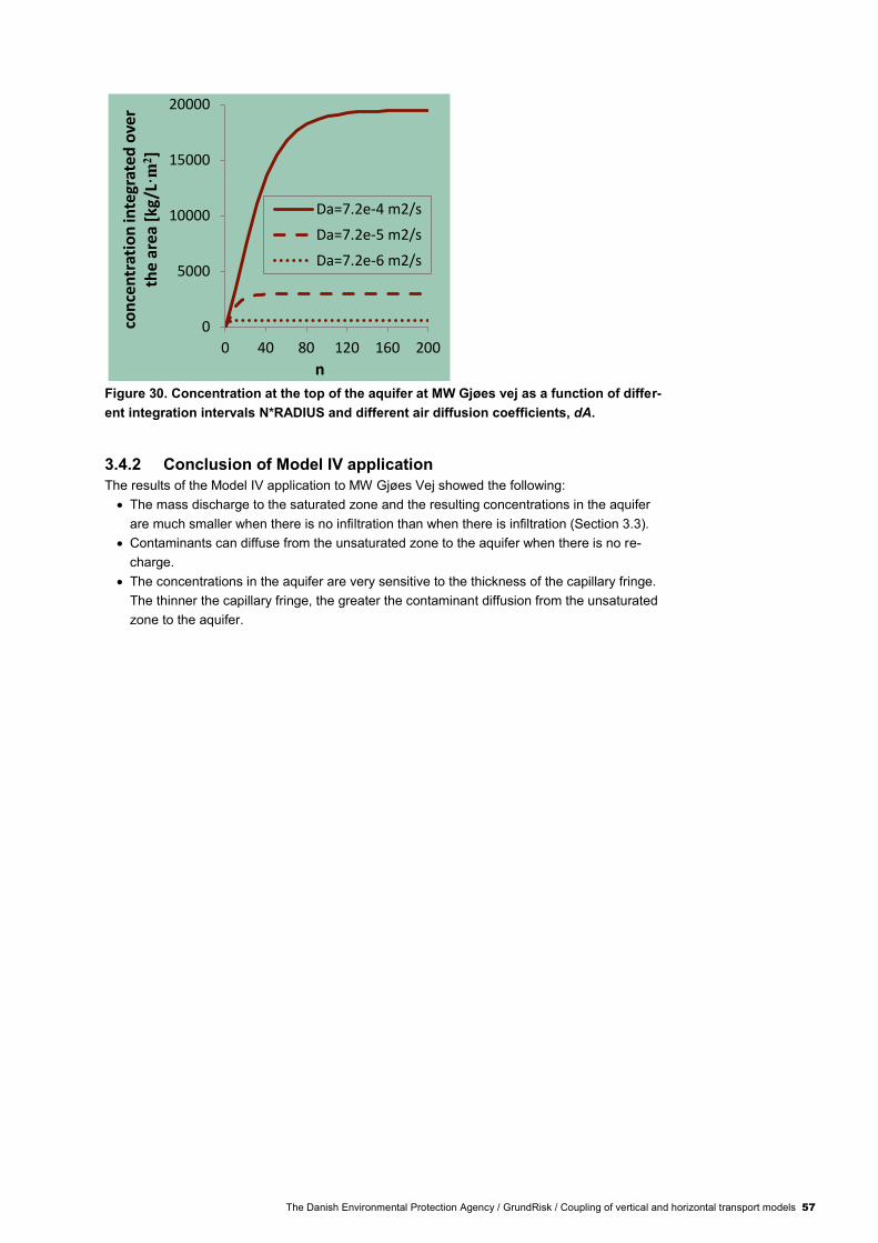
The Danish Environmental Protection Agency / GrundRisk / Coupling of vertical and horizontal transport models 57
Figure 30. Concentration at the top of the aquifer at MW Gjøes vej as a function of differ-
ent integration intervals N*RADIUS and different air diffusion coefficients, dA.
3.4.2 Conclusion of Model IV application
The results of the Model IV application to MW Gjøes Vej showed the following:
The mass discharge to the saturated zone and the resulting concentrations in the aquifer
are much smaller when there is no infiltration than when there is infiltration (Section 3.3).
Contaminants can diffuse from the unsaturated zone to the aquifer when there is no re-
charge.
The concentrations in the aquifer are very sensitive to the thickness of the capillary fringe.
The thinner the capillary fringe, the greater the contaminant diffusion from the unsaturated
zone to the aquifer.
0
5000
10000
15000
20000
0 40 80 120 160 200
con
cen
trat
ion
inte
grat
ed o
ver
the
are
a [k
g/L·m2]
n
Da=7.2e-4 m2/s
Da=7.2e-5 m2/s
Da=7.2e-6 m2/s
58 The Danish Environmental Protection Agency / GrundRisk / Coupling of vertical and horizontal transport models
References
Bear, J., 1972. Dynamics of Fluids in Porous Media. Elsevier, New York.
Broholm, K., Nilsson, B., Sidle, R.C., Arvin, E., 2000. Transport and biodegradation of creosote
compounds in clayey till, a field experiment. Journal of Contaminant Hydrology, 41: 239–
260.
Chambon, J., Bjerg, P.L., Binning, P.J. A risk assessment tool for contaminated sites in low-
permeability fractured media. Miljøstyrelsen (udkast 2010).
Chambon, J.C., Binning, P.J., Jørgensen, P.R., Bjerg, P.L., 2011. A risk assessment tool for
contaminated sites in low-permeability fractured media. Journal of Contaminant Hydrology,
124(1–4): 82-98.
Christophersen, M., Broholm, M., Mosbæk, H., Karapanagioti, H.K., Burganos, V.N., Kjeldsen,
P., 2005. Transport of hydrocarbons from an emplaced fuel source experiment in the va-
dose zone at Airbase Værløse, Denmark. Journal of Contaminant Hydrology, vol. 81, no. 1-
4, pp. 1– 33.
Christiansen, C., Wood, J. S. A., 2006. Environmental Fracturing in Clay Till Deposits, MSc
thesis, Institute of Environment & Resources – Technical University of Denmark.
Grathwohl, P., Klenk, I.D., Maier, U., Reckhorn, S.B.F., 2002. Natural attenuation of volatile
hydrocarbons in the unsaturated zone and shallow groundwater plumes: scenario-specific
modelling and laboratory experiment. Groundwater Quality: Natural and Enhanced Restora-
tion of Groundwater Pollution.
Hønning, J., Broholm, M.M., Bjerg, P.L., 2007. Role of diffusion in chemical oxidation of PCE in
a dual permeability system. Environmental Science & Technology. 41 (24), 8426 – 8432.
JAGG 2.0. http://mst.dk/virksomhed-myndighed/jord/it-vaerktoejer-til-vurdering-af-jord/
Jørgensen, P.R., McKay, L.D., Spliid, N.H., 1998. Evaluation of chloride and pesticide transport
in a fractured clayey till using large undisturbed columns and numerical modeling. Water
Resources Research. 34 (4), 539–553.
Jørgensen, P.R., Hoffmann, M., Kistrup, J.P., Bryde, C., Bossi, R., Villholth, K.G., 2002. Prefer-
ential flow and pesticide transport in a clay-rich till: field, laboratory, and modeling analysis.
Water Resources Research. 38 (11).
Jørgensen, T.H., Schondelmaier, A.M., Jepsen, J.D., Holm, O.V., 2003. Forureningsundersø-
gelse og afværgeprogram. Hovedrapport, Forurenet lokalitet nr. 461-169, Rugårdsvej 234
og 238 A-D, Odense, Fyns Amt, COWI.
Jørgensen, P.R., Helstrup, T., Urup, J., Seifert, S., 2004. Modelling of non-reactive solute
transport in fractured clayey till during variable flow rate and time. Journal of Contaminant
Hydrology, 68: 193-216.
Jørgensen, Torben H., Nielsen, L., Berger, H., Scheutz, C., Jakobsen, R., Bjerg, P.L., Durant,
N., Cox, E., Mossing, C.H., Jacobsen, C.S., Rasmussen, P., 2007a. Forundersøgelser til pi-
lotprojekt om stimuleret reduktiv deklorering. Miljøprojekt nr. 1146 2007. Miljøstyrelsen.
Jørgensen, Torben H., Nissen, L., Nielsen, L., Hansen, M.H., Scheutz, C., Jakobsen, R., Bjerg,
P.L., Durant, N., Cox, E., Mossing, C. H., Jacobsen, C. S., Rasmussen, P., 2007b. Pilotpro-
jekt om stimuleret reduktiv.
Klint, K.E.S., Nilsson, B., Troldborg, L., Jakobsen, P.R., 2013. A poly morphological landform
approach for hydrogeological applications in heterogeneous glacial sediments. Hydrogeolo-
gy Journal, 21(6), 1247–1264.
Krüger, (2004). MW Gjøes Vej, Reerslev, Supplerende undersøgelse af lerformation, Veolia
Water.
Lahvis, M.A., Baehr, A.L., Baker, R.J., 2004. Evaluation of volatilization as a natural attenuation
pathway for MTBE. Ground Water 42 (2), 258–267.
The Danish Environmental Protection Agency / GrundRisk / Coupling of vertical and horizontal transport models 59
Lahvis, M., Rehmann, L. 2000. Simulation of Transport of Methyl Tert-Butyl Ether (MTBE) to
Groundwater From Small-Volume Releases of Gasoline in the Vadose Zone. API Soil
Groundwater Research Bulletin. No. 10.
Lima, G.D., Sleep, B.E., 2007. The spatial distribution of eubacteria and archaea in sand-clay
columns degrading carbon tetrachloride and methanol. Journal of Contaminant Hydrology
94, 34 – 48.
Lu, C., Bjerg, P. L., Zhang, F., Broholm, M.M., 2011. Sorption of chlorinated solvents and deg-
radation products on natural clayey tills. Chemosphere, 83(11), 1467–1474.
McKay, L.D., Cherry, J.A., Gillham, R.W., 1993. Field experiment in a fractured clay till. 1. Hy-
draulic conductivity and fracture aperture. Water Resources Research Vol. 29, No. 4: 1149-
1162.
Miljøstyrelsen, 1998. Oprydning på forurenede lokaliteter, Hovedbind og Appendiks. Vejledning
fra Miljøstyrelsen nr. 6 og 7, 1998.
Miljøstyrelsen, 2002. Vejledning om overgangsplaner. Udarbejdelse af overgangsplaner for
bestående Deponeringsanlæg. Vejledning fra Miljøstyrelsen Nr. 5 2002.
Miljøstyrelsen, 2009a. A risk assessment tool for contaminated sites in low-permeability fractu-
red media. Environmental project No. 1786, 2015.
Miljøstyrelsen, 2009b. Model assessment of reductive dechlorination as remediation technology
for contaminant sources in fractured clay. Case studies. Delrapport III. Environmental Pro-
ject No. 1296 2009. Miljøprojekt.
Miljøstyrelsen, 2011. Fastlæggelse af oprensningskriterier for grundvandstruende forureninger.
Miljøprojekt nr.137, 2011.
Miljøstyrelsen, 2013. Manual for program til risikovurdering – JAGG 2.0. Miljøprojekt nr. 1508,
2013.
Miljøstyrelsen, 2014. Liste over kvalitetskriterier i relation til forurenet jord og kvalitetskriterier for
drikkevand. Opdateret maj 2014. Miljøministeriet, Miljøstyrelsen.
Miljøstyrelsen, 2015. A risk assessment tool for contaminated sites in low-permeability fractured
media. Environmental project No. 1786.
Miljøstyrelsen, 2016a. JAGG 2 - Vertikal transport ned til førstkommende betydende magasin.
Miljøprojekt nr. 1828, 2016.
Miljøstyrelsen, 2016b. GrundRisk Beregningsmodel til risikovurdering af grundvandstruende
forureninger. Miljøprojekt nr. 1865, 2016.
Niras, 2009. MW Gjøes Vej, Reerslev, Indsamling, systematisering og vurdering af data, Kon-
cern Miljø, Region Hovedstaden.
Parker, B.L., Gillham, R.W., Cherry, J.A., 1994. Diffusive disappearance of immiscible-phase
organic liquids in fractured geologic media. Ground Water. 32 (5), 805–820.
Scheutz, C., Durant, N.D., Dennis, P., Hansen, M.H., Jørgensen, T., Jakobsen, R., Cox, EE.,
Bjerg, P.L., 2008. Concurrent Ethene Generation and Growth of Dehalococcoides Contain-
ing Vinyl Chloride Reductive Dehalogenase Genes During an Enhanced Reductive Dechlo-
rination Field Demonstration. Environmental Science & Technology 42 (24), s. 9302-9309.
Scheutz, C., Broholm, M.M., Durant, N.D., Weeth, E.B., Jørgensen, T.H., Dennis, P., Jacobsen,
C.S., Cox, E.E., Chambon, J.C., Bjerg, P.L., 2010. Field evaluation of biological enhanced
reductive dechlorination of chloroethenes in clayey till. Environmental Science & Technolo-
gy. 44 (13), 5134–5141.
Schwarzenbach, R.P., Gschwend, P.M., Imboden, D.M., 1993. Environmental Organic Chemis-
try. John Wiley & Sons, INC.
Spiegel, M.R. (1968): Mathematical handbook of formulas and tables. Schaum’s outline series.
McGraw-Hill.
Sun, Y., Petersen, J.N., Clement T.P., 1999a. Analytical solutions for multiple species reactive
transport in multiple dimensions, Journal of Contaminant Hydrology, 35(4), 429-440.
Sun, Y., Petersen, J.N., Clement T.P., Skeen R.S., 1999b. Development of analytical solutions
for multispecies transport with serial and parallel reactions, Water Resources Research,
35(1), 185-190.

60 The Danish Environmental Protection Agency / GrundRisk / Coupling of vertical and horizontal transport models
Tang, D.H., Frind, E.O., Sudicky, E.A., 1981. Contaminant transport in fractured porous-media
— analytical solution for a single fracture. Water Resources Research. 17 (3), 555–564.
Troldborg, M., Binning, P.J., Nielsen, S., Kjeldsen, P., Christensen, A.G., 2009. Unsaturated
zone leaching models for assessing risk to groundwater of contaminated sites. Journal of
hydrology. Volume 105, Issues 1–2.
Van Genuchten, M.T, Alves, W.J., 1982. Analytical Solutions of the One Dimensional Convec-
tive-Dispersive Solute Transport Equation. United States Department of Agriculture. Agricul-
tural research Service. Technical Bulletin, Number 1661.
Videncenter for Jordforurening, 2008. SprækkeJAGG. Regneark til risikovurdering af sprækker i
moræneler Teknik og Administration Nr. 2, 2008.
Wexler, E.L., 1992. Analytical Solutions for one-, two- and three-dimensional solute transport in
ground-water systems with uniform flow. Chapter B7 in Techniques of Water-Resources In-
vestigations of the United States Geological Survey. Book 3 Applications of Hydraulics. U.S.
Department of the interior. U.S. Geological Survey. United States Government Printing Of-
fice, 1992.
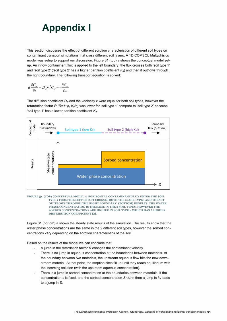
The Danish Environmental Protection Agency / GrundRisk / Coupling of vertical and horizontal transport models 61
Appendix I
This section discusses the effect of different sorption characteristics of different soil types on
contaminant transport simulations that cross different soil layers. A 1D COMSOL Multyphisics
model was setup to support our discussion. Figure 31 (top) a shows the conceptual model set-
up. An inflow contaminant flux is applied to the left boundary, the flux crosses both ‘soil type 1’
and ‘soil type 2’ (‘soil type 2’ has a higher partition coefficient Kd) and then it outflows through
the right boundary. The following transport equation is solved:
2w ww w
C CR D C v
t x
The diffusion coefficient Dw and the veolocity v were equal for both soil types, however the
retardation factor R (R=1+ρb·Kd/n) was lower for ‘soil type 1’ compare to ‘soil type 2’ because
‘soil type 1’ has a lower partition coefficient Kd.
FIGURE 31. (TOP) CONCEPTUAL MODEL A HORIZONTAL CONTAMINANT FLUX ENTER THE SOIL
TYPE 1 FROM THE LEFT END, IT CROSSES BOTH THE 2 SOIL TYPES AND THEN IT
OUTFLOWS THROUGH THE RIGHT BOUNDARY. (BOTTOM) RESULTS. THE WATER
PHASE CONCENTRATION IS THE SAME IN THE 2 SOIL TYPES, HOWEVER THE
SORBED CONCENTRATIONS ARE HIGHER IN SOIL TYPE 2 WHICH HAS A HIGHER
DISTRIBUTION COEFFICIENT Kd.
Figure 31 (bottom) a shows the steady state results of the simulation. The results show that the
water phase concentrations are the same in the 2 different soil types, however the sorbed con-
centrations vary depending on the sorption characteristics of the soil.
Based on the results of the model we can conclude that:
- A jump in the retardation factor R changes the contaminant velocity.
- There is no jump in aqueous concentration at the boundaries between materials. At
the boundary between two materials, the upstream aqueous flow hits the new down-
stream material. At that point, the sorption sites fill up until they reach equilibrium with
the incoming solution (with the upstream aqueous concentration).
- There is a jump in sorbed concentration at the boundaries between materials. If the
concentration c is fixed, and the sorbed concentration S=kd·c, then a jump in kd leads
to a jump in S.
Soil type 1 (low Kd) Soil type 2 (high Kd)
Boundaryflux (inflow)
Boundaryflux (outflow)
Stea
dy-
stat
eco
nce
ntr
atio
ns
Water phase concentration
Sorbed concentration
Co
nce
ptu
alm
od
elR
esu
lts
x

62 The Danish Environmental Protection Agency / GrundRisk / Coupling of vertical and horizontal transport models
- The two materials will have different total concentrations (total contaminant
mass/volume) at steady-state because of the change in sorption characteristics.
Environmental
Protection Agency
Strandgade 29
DK-1401 København K
www.mst.dk
GrundRisk – Coupling of vertical and horizontal transport models
This report presents the development of the GrundRisk model for contaminated site
risk assessment. GrundRisk consists of 5 models, each simulating the contaminant
transport from a contaminant source to an underlying aquifer. Each model consist of
a vertical transport model (based on the models presented in Miljøstyrelsen (2016a))
coupled to a horizontal transport model (Miljøstyrelsen (2016b). This report focuses
on the coupling between the vertical and horizontal models.