coupled currents in cosmic strings fileoutline 1. how do cosmic strings arise? 2. some numbers on...

Coupled Currents in Cosmic Strings

Marc Lilley

GRεCO, Institut d’Astrophysique de Paris

April 28, 2009

Marc Lilley Coupled Currents in Cosmic Strings

Outline

1. How do cosmic strings arise?

2. Some numbers on cosmic strings.

3. How do cosmic strings evolve?

4. Cosmic strings in field theory.

5. Currents in cosmic strings.

6. Cosmic strings in the worldsheet approach.

7. Coupled currents in cosmic strings.

8. Conclusions.


How do cosmic strings arise? (Kibble, ’81)

Universe expands from a hot thermal local equilibrium state

It is assumed that at high energy, interactions are unified (enhanced

symmetry)

With the cooling, spontaneous symmetry breaking occurs

This is the Higgs mechanism

For a field with a local U(1) gauge symmetry Φ, the effective potential atT = 0 is

V (Φ) =λ

8

(|Φ|2 − η2

)2On distance larger than the horizon scale (causally disconnected), the phase(χ) choice is uncorrelated

The phase is single-valued and a continuous function:

On a closed path, ∆χ = 2πn

⇒ if n 6= 0, there exists a singular point within the closed path: Φ = 0

⇒ strings are either infinite in length or loopsMarc Lilley Coupled Currents in Cosmic Strings

Some facts on cosmic strings

Correlation length: ξ ∼ m−1h ,

String loop radius: m−1h

Energy per unit length: U ∼ η2

For grand unification scales: 1015 tons/cm

Number density: nb ∼ ξ−3

80% of strings at formation are of length (radius) > horizon⇒ At first they grow!

Probability for intercommutation is of order 1

Generates a population of loops

Gravitational energy loss

Shrink under the effect of string tension(note: stabilizing mechanisms exist, c. f. , later)


Cosmological Considerations

The spectrum of primordial fluctuations for cosmic stringsdisagrees with CMB data (Durrer et al., ’96, Bouchet et al., ’01)

SUSY D-term inflation models ⇒ cosmic “D-term” strings(Jeannerot et al. ’03)

Tension between particle physics model building and cosmologicaldata

⇒ Constraints

Renewed interest:

Brane inflationary model building

D-term and F strings produced at the end of brane inflation

Conjecture: ⇔ D-strings (Dvali et al., ’04)

⇒ Distinction: topological vs. string theory stringsMarc Lilley Coupled Currents in Cosmic Strings

Nambu-Goto Strings I

Abelian Higgs model (Nielsen & Olesen, ’73):

LH = −Dµφ∗Dµφ− 1

4FµνF

µν −λφ2

(|φ|2 − η2

)2Fµν = ∂µAν − ∂νAµ, Dµ = ∂µ + ieAµ

In a straight and static string with cylindricalsymmetry:

φ = ϕ(r)e iχ (with χ some angle)

Aµ =1

e2

jµ|φ|2− 1

e∂µχ

z

r

θ

STRING

Electromagnetic flux (⇒ stability against relaxation to |η|):

Φ =

∫Fµνdσµν =

∮`Aµdxµ = −

∮`

∂µχ

edxµ = −2πn

e


Nambu-Goto Strings II

We assume thatχ = nθ ⇒ φ = ϕ(r)e inθ

We obtain a flux tube:

Aµ = Aθ(r)δµθ ⇒ Fµν = ∂rAθ(r)δµrδνθ

In the worldsheet description:

Energy-momentum tensor in flat spacetime in the thin string limit(Peter, 1994)

Tµν

=

∫Tµνd2x⊥ ⇒ T tt , T zz

Nambu-Goto action:

S = α

∫d2ξ√−γ, ds2 = gµνdxµdxν = γabdξadξb (a = 0, 1)

Straight and static configuration, ξ0 = t and ξ1 = z :

T tt = T zz ⇒ U = T


Superconducting Strings (Witten, ’85)

Couple the string to a field Σ with U(1)local:

L = LH − DµΣ∗DµΣ− 1

4HµνH

µν − V (Σ, φ)

V (Σ, φ) = βσ(|φ|2 − η2

)|Σ|2 + m2Σ2 +

λ

2|Σ|4

Hµν = ∂µBν − ∂νBµ, Dµ = ∂µ + iqBµ

Consider a of string with local cylindrical symmetry:

Σ = σ(r)e iψ(t,z), jµ = σ2(∇µψ + qBµ), ψ(t, z) = ωt − kz∮dψdζ

dζ = 2πm ⇒ dψ

dζ=

m

R

If m 6= 0, then the string is superconducting...Also note:

U 6= T


Neutral strings (Peter, ’92)

Key effect of currents on the string is mechanical (Davis & Shellard, ’88)

We can consider two frames (Carter, ’90):

a rotating frame (Tµν diagonal)

a local stationary frame in which we have J = 2πR2T 01

⇒ Equilibrium configurations for R2Ω2 = T/U (Ω: ang. velocity)

Are they really stable?

Witten string model is not stricly local:

the gauge field Bµ diverges logarithmically with r ,

leads to divergent integrals,

necessitates the introduction of characteristic and cut-offscales.

Neutral limit:

coupling constant q → 0,

mechanical properties of the string well reproduced!


State parameter, electric & magnetic strings (Carter, ’89)

A choice of field theory fixes all parameters expect k and ωCan define

L(w) =

∫Ld2x⊥, w = k2 − ω2 = gµν∇µψ∇νψ

where w is the only possible Lorentz scalar.

Introduce the first fundamental tensor:

ηµν = hab ∂Xµ

∂ξa∂X ν

∂ξb

If w > 0 (spacelike),√

wvµ = ηµν∇νψ (magnetic string), vµvµ = 1

If w < 0 (timelike),√−wuµ = ηµν∇νψ (electric string), uµuµ = −1

Define preferred frame:

ηµν = −uµuν + vµvν

⇒ Tµν diagonalMarc Lilley Coupled Currents in Cosmic Strings

Properties of the worldsheet & of the currents (Carter, ’89)

Definitions

Orthogonal projector ⊥µν= gµν − ηµν

Antisymmetric tensor εµρενρ = ηµν

Worldsheet derivative ∇µ = ηνµ∇ν

Extrinsic curvature K ρµν = ησµ∇νη

ρσ

Conservation equations:

Integrability of the worldsheet: K ρ[µν] = 0

Conservation of Tµν

: ∇µTµν

= 0

Current conservation: ∇µcµ = 0

Irrot. : cµ ∝ ∇µψ ⇔ εµν∇µ(∇νψ) = 0

Note: The geometry of the string worldsheet decouples from itsinternal dynamics for small perturbations⇒ split conservation equations in ⊥ and ‖ components


Stability

The idea is to understand if the straight and static string is stableunder small perturbations to the currents

Perturbed current:

δ (cµ) = δcµeiχ, ∇µχ = kµ, ω = kµu

µ, k = −kµvµ

Perturbations do not grow if χ ∈ RTransverse perturbations (⊥νµ)

c2T =

ω2T

k2T

=T

U⇒ T > 0

Longitudinal perturbations (ηνµ)

c2L =

ω2L

k2L

= −dT

dU⇒ dT

dU< 0


Electric/magnetic Duality (Carter, ’89)

Define: K = −2dLdw

= −∫σ(r)2dx⊥

Then:

Ttt

= ω2

∫σ(r)2d⊥x − L, T

zz= k2

∫σ(r)2d⊥x + L

If w < 0 (electric)⇒ w = −ω2 and k = 0:

Ttt

= −wK − L = −L = U, Tzz

= L = −T

If w > 0 (magnetic)⇒ w = k2 and ω = 0:

Tzz

= wK + L = L = −T , Ttt

= −L = U

In short:

T = −L, U = −L (w < 0) T = −L, U = −L (w > 0)

⇒ U − T = |w |K⇒ Simple expressions for cT and cL


String model (Carter & Peter, ’95)

Electric (w < 0)

FT indicates 1st order pole in K (Phase

frequency threshold, w = −m2)

L(w) = −mh2− m2

2ln(

1 +w

m2

)

-0.03 -0.02 -0.01 0 0.01 0.02 0.03 0.04~ν

4.9

5.0

5.1

5.2

U/η2

T/η2

Magnetic (w > 0)

L(w) = −mh2 − w

2

(1 +

w

m2

)−1

-0.02 -0.01 0 0.01 0.02 0.03 0.04~ν

5.0

4.9

5.1

5.2

U/η2

T/η2


Microscopic physics for N=2 currents I

Can we extend the formalism to more than one condensate?

What are the similarities and differences with the onecondensate case?

Does it lead to new instabilities? What is the effect of the

coupling between the N additional fields?

Can the numerical results be reproduced with an analyticmodel?


Microscopic physics for N=2 currents II

Lagrangian:

L = −1

2(DµH)† (DµH)− 1

4CµνC

µν− 1

2∂µΦ?∂µΦ− 1

2∂µΣ?∂µΣ−V

DµH = (∂µ + iqCµ)H and Cµν ≡ ∂µCν − ∂νCµPotential:

V =λ

8(|H|2 − η2)2 +

1

2m2φ|Φ|2 +

1

2m2σ|Σ|2 +

1

2

(|H|2 − η2

) (fφ|Φ|2 + fσ|Σ|2

)+

1

4λφ|Φ|4 +

1

4λσ|Σ|4 +

g

2|Φ|2|Σ|2


Ansatze, L, Tab

, U , T and state parameters

Ansatze:

H(xα) = h(r)einθ, Cµ(xα) =Q(r)− n

qδθµ

Φ(xα) = φ(r)eiψφ , Σ(xα) = σ(r)eiψσ

L and K:

L → L = L(wφ,wσ)

Ki = 2dLdwi

3 L-I state parameters:

wσ = k2σ − ω2

σ

wσ = k2φ − ω2

φ

x = kσkφ − ωσωφ

Diagonalize Tµν

:

U = A + B

T = A− B

A : A (wφ,wσ, x ,Kφ,Kσ)

B : B (wφ,wσ, x ,Kφ,Kσ)


Field theory side: field profiles

Results of numerical relaxation method for wσ = wφ = 0

FT physics independent of x

fix microscopic parameters

choose wi ’s

switch to dimensionless variables X , Y , Z , Q

weak coupling

0.0 5.0 10.0 15.0 20.0ρ

0

0.5

1.0

1.5

2.0

2.5

3.0

Y(ρ)

X(ρ)Q(r)

~g2= ~g

2

2=0.05 γφγσ

Z(ρ)

strong coupling

0.0 5.0 10.0 15.0 20.0ρ

0

0.5

1.0

1.5

2.0

2.5

3.0

Y(ρ)

X(ρ)Q(r)

~g2= ~g

3

2= 0.5 γφγσ

Z(ρ)


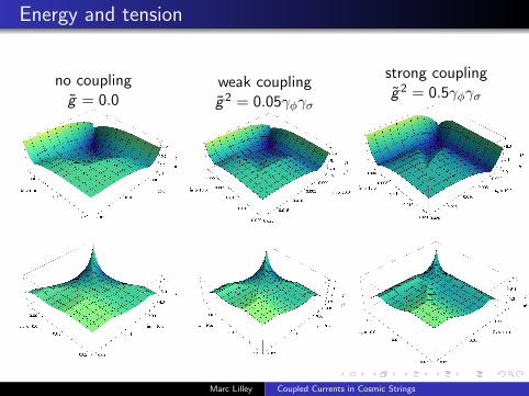
Energy and tension

no couplingg = 0.0

weak couplingg2 = 0.05γφγσ

strong couplingg2 = 0.5γφγσ


Comparison with simplified model

-0.02 -0.01 0 0.01 0.02 0.03~ν

4.9

5.0

5.1

5.2

4.8

U/η2

T/η2

-0.02 -0.01 0 0.01 0.02 0.03~ν

4.9

5.0

5.1

5.2

4.8

U/η2

T/η2

-0.02 -0.01 0 0.01 0.02 0.03~ν

4.9

5.0

5.1

5.2

4.8

U/η2

T/η2

-0.02 -0.01 0 0.01 0.02 0.03~ν

4.9

5.0

5.1

5.2

4.8

U/η2

T/η2

-0.02 -0.01 0 0.01 0.02 0.03~ν

4.9

5.0

5.1

5.2

4.8

U/η2

T/η2

-0.02 -0.01 0 0.01 0.02 0.03~ν

4.9

5.0

5.1

5.2

4.8

U/η2

T/η2

-0.02 -0.01 0 0.01~ν

4.9

5.0

5.1

5.2

U/η2

T/η2

-0.02 -0.01 0 0.01~ν

4.9

5.0

5.1

5.2

U/η2

T/η2

-0.02 -0.01 0 0.01~ν

4.9

5.0

5.1

5.2

U/η2

T/η2


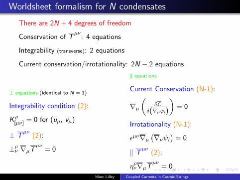
Worldsheet formalism for N condensates

There are 2N + 4 degrees of freedom

Conservation of Tµν

: 4 equations

Integrability (transverse): 2 equations

Current conservation/irrotationality: 2N − 2 equations

⊥ equations (Identical to N = 1)

Integrability condition (2):

K ρ[µν] = 0 for (uµ, vµ)

⊥ Tµν

(2):

⊥ρν ∇µTµν

= 0

‖ equations

Current Conservation (N-1):

∇µ(

δLδ(∇µϕi)

)= 0

Irrotationality (N-1):

εµν∇µ(∇νψi

)= 0

‖ Tµν

(2):

ηρν∇µTµν

= 0


Reference frame

No preferred reference frame in the sense of the single current case

If one current is made colinear w/ uµ or vµ, the other is not!

⇒ Conditions for stability are a priori different for N > 1

Project the currents onto the lightlike directions:

Places currents on an equal footing,

Is a convenient choice.

Introduce

e+iµ =

1

2

[diµ − (−1)iενµdiν

]e−iµ =

1

2wi

[diµ + (−1)iενµdiν

]with diµ = εµν∇νψi , the most meaningful quantity

Note: 4e±i for 2 lightlike directions:

⇒ provides a convenient way to relate the currents


Stability for N = 2 currents

Reminder: the perturbation equation for transverse perturbationsdecouples from perturbations in the currents

⊥ perturbations

c2T =

ω2T

k2T

=T

U⇒ T > 0

⊥ microscopic condition!

x2 ≤ 1

KφKσ

[A2 −

(1

2wφKφ −

1

2wσKσ

)2]

‖ perturbations

∇µ(Kij∇µψj

)= 0

εµν∇µ(∇νψi

)= 0

⇒ Set of 4 coupled equations in

the currents and the perturbations

‖ stability

Determinant:c0 + c1ξ + c2ξ

2 + c3ξ3 + c4ξ

4 = 0

ξ =−ζe−1t +e−1z

−ζe−2t +e−2z

ζ2 =ω2

t

k2z

6= −dT

dU


Stability of simplified model

L for decoupled fields:

L = L1(χ1) + L2(χ2) + m2

‖ stability:

Decoupling of longitudinal modes ⇒ −m2i ≤ wi ≤ m2

i

⊥ stability:

T > 0⇒ x2 ≤ xlim

w1w2 ≥ 0

x2lim = w1w2(U1−m2+T2)(U2−m2+T1)

(U1−T1)(U2−T2)

w1w2 ≤ 0

x2lim =

|w1w2|(T1+T2−m2)(U1+U2−m2)(U1−T1)(U2−T2)


Stability: Simplified model vs. numerical result

w1 < 0, w2 < 0

w1 > 0, w2 > 0

w1 < 0, w2 > 0

w1 > 0, w2 < 0


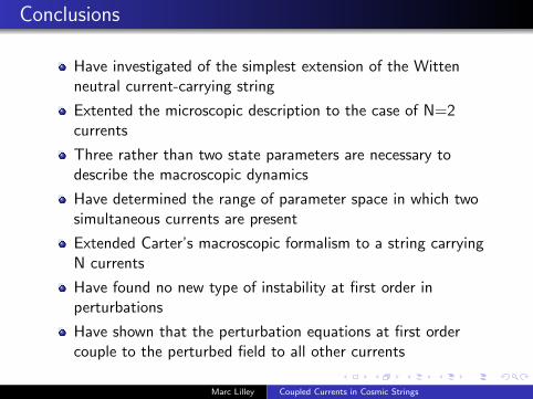
Conclusions

Have investigated of the simplest extension of the Wittenneutral current-carrying string

Extented the microscopic description to the case of N=2currents

Three rather than two state parameters are necessary todescribe the macroscopic dynamics

Have determined the range of parameter space in which twosimultaneous currents are present

Extended Carter’s macroscopic formalism to a string carryingN currents

Have found no new type of instability at first order inperturbations

Have shown that the perturbation equations at first ordercouple to the perturbed field to all other currents


Conclusions

Have shown that the stability of transverse modes has a directinterpretation in terms of the scalar product of the phasegradients (i.e., in terms of x)

Have investigated the possibility to reproduce the results usinga simplified model based on a log-fuction for w < 0 and arational function for w > 0 for different values of the couplingg .

The results are consistent with expectations1 U and T are best reproduced at weak coupling or when one

current largely dominates2 Reproducing the stability in the 0 and weak coupling regime is

okay3 Reproducing the stability in the strong coupling regime fails to

capture much of the physics


coupled currents in cosmic strings fileoutline 1. how do cosmic strings arise? 2. some numbers on...

Documents