Counterparty risk and funding:

the four wings of the TVA

Stephane Crepey, Remi Gerboud, Zorana Grbac and Nathalie Ngor

Laboratoire Analyse et Probabilites

Universite d’Evry Val d’Essonne

91037 Evry Cedex, France

April 10, 2013

Abstract

The credit crisis and the ongoing European sovereign debt crisis have highlighted thenative form of credit risk, namely the counterparty risk. The related credit valuationadjustment (CVA), debt valuation adjustment (DVA), liquidity valuation adjustment(LVA) and replacement cost (RC) issues, jointly referred to in this paper as total valua-tion adjustment (TVA), have been thoroughly investigated in the theoretical papers [9]and [10]. The present work provides an executive summary and numerical companionto these papers, through which the TVA pricing problem can be reduced to Markovianpre-default TVA BSDEs. The first step consists in the counterparty clean valuation ofa portfolio of contracts, which is the valuation in a hypothetical situation where thetwo parties would be risk-free and funded at a risk-free rate. In the second step, theTVA is obtained as the value of an option on the counterparty clean value process calledcontingent credit default swap (CCDS). Numerical results are presented for interest rateswaps in the Vasicek, as well as in the inverse Gaussian Hull-White short rate model,which allows also to assess the related model risk issue.

Keywords: Counterparty risk, credit valuation adjustment (CVA), debt valuation adjust-ment (DVA), liquidity valuation adjustment (LVA), backward stochastic differential equa-tion (BSDE), interest rate swap.

1 Introduction

The credit crisis and the ongoing European sovereign debt crisis have highlighted the nativeform of credit risk, namely the counterparty risk. This is the risk of non-payment of promisedcash-flows due to the default of the counterparty in a bilateral OTC derivative transaction.The basic counterparty risk mitigation tool is a credit support annex (CSA) specifying avaluation scheme of a portfolio of contracts at the default time of a party. In particular, thenetting rules which will be applied to the portfolio are specified, as well as a collateralizationscheme similar to margin accounts in futures contracts.

By extension counterparty risk is also the volatility of the price of this risk, this pricebeing known as credit valuation adjustment (CVA); see [21], [3], [1]. Moreover, as banksthemselves have become risky, counterparty risk must be understood in a bilateral perspec-tive, where the counterparty risk of the two parties is jointly accounted for in the modeling.

2

Thus, in addition to the CVA, a debt valuation adjustment (DVA) must be considered. Inthis context the classical assumption of a locally risk-free asset which is used for financ-ing purposes of the bank is not sustainable anymore. This raises the companion issue ofproper nonlinear accounting of the funding costs of a position and a corresponding liquidityvaluation adjustment (LVA). The last related issue is that of replacement cost (RC) cor-responding to the fact that at the default time of a party the contract is valued by theliquidator according to a CSA valuation scheme which can fail to reflect the actual value ofthe contract at that time.

The CVA/DVA/LVA/RC intricacy issues, jointly referred to henceforth as TVA (fortotal valuation adjustment), were thoroughly investigated in the theoretical papers [9],[10], [2] and [5]. The present work is a numerical companion paper to [9] and [10] and isorganized as follows. Section 2 provides an executive summary of the two papers. Section 3describes various CSA specifications. In Sections 4 and 5 we present clean valuation (cleanof counterparty risk and funding costs) and TVA computations in two simple models forinterest rate derivatives. We show in a series of practical examples how CVA, DVA, LVAand RC can be computed in various situations (note they have to be computed jointly asthey depend on each other), and we also assess the related model risk issue.

2 TVA representations

2.1 Setup

We consider a netted portfolio of OTC derivatives between two defaultable counterparties,generically referred to as the “contract between the bank and her counterparty”. Thecounterparty is most commonly a bank as well. Counterparty risk and funding cash-flowscan only be considered at a netted and global level, outside the scope of different businessdesks. Consequently, the price Π of the contract must be computed as a difference betweenthe clean price P provided by the relevant business desk and a correction Θ computedby the central TVA desk. By price we mean here the cost for the bank of margining,hedging and funding (“cost of hedging” for short). By clean price we mean the price ofthe contract computed without taking into account counterparty risk and excess fundingcosts. Symmetrical considerations apply to the counterparty, but with non-symmetricaldata in the sense of hedging positions and funding conditions. As a consequence and dueto nonlinearities in the funding costs, the prices (costs of hedging) are not the same for thetwo parties. For clarity we focus on the bank’s price in the sequel.

We denote by T the time horizon of the contract with promised dividends dDt fromthe bank to her counterparty. Both parties are defaultable, with respective default timesdenoted by θ and θ. This results in an effective dividend stream dCt = JtdDt, whereJt = 1t<τ with τ = θ ∧ θ. One denotes by τ = τ ∧ T the effective time horizon ofthe contract as there are no cash-flows after τ . The case of unilateral counterparty risk(from the perspective of the bank) can be recovered by letting θ ≡ ∞. After having soldthe contract to the investor at time 0, the bank sets-up a collateralization, hedging andfunding portfolio (“hedging portfolio” for short). We call an external funder of the bank(or funder for short) a generic third-party, possibly composed in practice of several entitiesor devices, insuring funding of the position of the bank. This funder, assumed default-freefor simplicity, thus plays the role of “lender/borrower of last resort” after exhaustion of theinternal sources of funding provided to the bank via the dividend and funding gains on herhedge, or via the remuneration of the collateral account.

3

The full model filtration is given as G = F∨Hθ∨Hθ, where F = (Ft)0≤t≤T is a reference

filtration and Hθ = (Hθt )0≤t≤T and Hθ = (Hθt )0≤t≤T , with Hθt = σ(θ ∧ t) and Hθt = σ(θ ∧ t).All filtrations are assumed to satisfy the usual conditions. A probability space (Ω,GT ,P),where P is some risk-neutral pricing measure, is fixed throughout. The meaning of a risk-neutral pricing measure in this context, with different funding rates in particular (see [9]),will be specified by martingale conditions introduced below in the form of suitable pricingbackward stochastic differential equations (BSDEs); see [13] for the seminal reference infinance.

Remark 2.1 Even though it will not appear explicitly in this paper, a pricing measuremust also be such that the gain processes on the hedging assets follow martingales; see [9].

Moreover, we assume that F is immersed into G in the sense that an F-martingale stoppedat τ is a G-martingale.

Remark 2.2 As discussed in [10], this basic assumption precludes major wrong-way riskeffects such as the ones which occur with counterparty risk on credit derivatives. In partic-ular, under these assumptions an F-adapted cadlag process cannot jump at τ. We refer to[8] for an extension of the general methodology of this paper beyond the above immersionsetup to incorporate wrong-way risk when necessary.

2.2 Data

We denote by rt the OIS rate at time t ∈ [0, T ], where OIS stands for an Overnight IndexedSwap, the best market proxy of a risk-free rate. By rt = rt + γt we denote the credit-risk adjusted rate, where γt is the F-hazard intensity of τ , which is assumed to exist. Letβt = exp(−

∫ t0 rsds) and βt = exp(−

∫ t0 rsds) stand for the corresponding discount factors.

Furthermore, Et and Et stand for the conditional expectations given Gt and Ft, respectively.The clean value process Pt of the contract with promised dividends dDt is defined, fort ∈ [0, τ ], as

βtPt := Et(∫ T

tβsdDs

)= Et

[ ∫ τ

tβsdDs + βτPτ

](1)

by immersion of F into G.Effectively, promised dividends dDt stop being paid at τ (if τ < T ), at which time

the last terminal cash-flow R paid by the bank closes out her position. Let an F-adaptedprocess Q represent the (predictable) CSA value process of the contract, and an F-adaptedprocess Γ stand for the value process of a CSA (cash) collateralization scheme. We denoteby π a real number meant to represent the wealth of the hedging portfolio of the bank in thefinancial interpretation. The close-out cash-flow R = R(π) is in fact twofold, decomposinginto a close-out cash-flow Ri from the bank to the counterparty, minus, in case of default ofthe bank, a cash-flow Rf = Rf (π) from the funder to the bank (depending on π). These twocash-flows are respectively derived from the algebraic debt χ of the bank to her counterpartyand X(π) of the bank to her funder, modeled at time τ as

χ = Qτ − Γτ , X(π) = −(π − Γτ−). (2)

The close-out cash-flow, if τ < T , is then modeled as R(π) = Ri − 1τ=θRf (π), where

Ri = Γτ + 1τ=θ

(ρχ+ − χ−

)− 1τ=θ

(ρχ− − χ+

)− 1θ=θχ

Rf (π) = (1− r)X+(π),(3)

4

in which ρ and ρ stand for recovery rates between the two parties, and r stands for a recoveryrate of the bank to her funder. The Gτ -measurable exposure at default is defined in termsof R as

ξ(π) := Pτ −R(π) = Pτ −Qτ + 1τ=θ

((1− ρ)χ+ + (1− r)X+(π)

)− (1− ρ)1τ=θχ

−, (4)

where the second equality follows by an easy algebraic manipulation.

Remark 2.3 Under certain specifications considered below, Ri and Γ also depend on πvia Q. Such additional dependence essentially does not alter the flow of arguments and istherefore omitted for notational simplicity.

We now consider the cash-flows required for funding the bank’s position, meant in thesense of the contract and its hedging portfolio altogether. For simplicity we stick to themost common situation where the hedge is self-funded as swapped and/or traded via repomarkets (see [9]). The OIS rate rt is used as a reference for all other funding rates, whichare thus defined in terms of corresponding bases to rt. Given such bases bt and bt relatedto the collateral posted and received by the bank, and λt and λt related to external lendingand borrowing, the funding coefficient gt(π) is defined by

gt(π) = (btΓ+t − btΓ

−t ) + λt (π − Γt)

+ − λt (π − Γt)− . (5)

Then (rtπ + gt(π))dt represents the bank’s funding cost over (t, t + dt), depending on thewealth π.

Remark 2.4 A funding basis is typically interpreted as a combination of liquidity andcredit risk; see [14] and [11]. Collateral posted in foreign currency and switching currencycollateral optionalities can also be accounted for by suitable amendments to b and b; see[15] and [20].

2.3 BSDEs

With the data ξ and g specified, the TVA process Θ can be implicitly defined on [0, τ ] as thesolution to the following BSDE, posed in integral form and over the random time interval[0, τ ]: For t ∈ [0, τ ],

βtΘt = Et[βτ1τ<T ξ(Pτ −Θτ−) +

∫ τ

tβsgs(Ps −Θs)ds

]. (6)

The reader is referred to [10, Proposition 2.1] for the derivation of the TVA BSDE (6). Inthis paper for simplicity of presentation we take (6) as the definition of the TVA.

The practical conclusion of [10] is that one can even adopt a simpler “reduced, pre-default” perspective in which defaultability of the two parties only shows up through theirdefault intensities; see Proposition 2.5 below and equation (3.8) in [10]. For t ∈ [0, T ] andπ ∈ R let

χt = Qt − Γt

ξt(π) = (Pt −Qt) + pt((1− ρt)χ+

t + (1− r)(π − Γt)−)− pt(1− ρt)χ−t , (7)

in which

pτ = P(τ = θ | Gτ−) , pτ = P(τ = θ | Gτ−).

Note that in case of unilateral counterparty risk, we have θ ≡ ∞ and consequently, pτ = 0,pτ = 1.

5

Proposition 2.5 (TVA reduced-form representation) One has Θ = Θ on [0, τ) andΘτ = 1τ<T ξ, where

βtΘt = Et[ ∫ T

tβs(gs(Ps − Θs) + γsξs(Ps − Θs)

)ds], (8)

for t ∈ [0, T ].

Remark 2.6 This assumes that the data of (8) are in F, a mild condition which can alwaysbe met by passing to F-representatives (or pre-default values) of the original data.

Remark 2.7 For r = 1 the exposure at default ξ does not depend on π, and in case of alinear funding coefficient given as gt(P − ϑ) = g0

t (P ) − λ0tϑ, for some g0 and λ0, the TVA

equations (6) and (8) respectively boil down to the explicit representations

β0t Θt = Et

[β0τ1τ<T ξ +

∫ τt β

0sg

0s(Ps)ds

](9)

β0t Θt = Et

[ ∫ Tt β0

s

(g0s(P

0s ) + γsξ

0s

)ds]. (10)

Here the funding-adjusted discount factors are

β0t = exp(−

∫ t

0(rs + λ0

s)ds) , β0t = exp(−

∫ t

0(rs + λ0

s)ds)

and ξ0t in (10) is given by

ξ0t = (Pt −Qt) + pt(1− ρt)χ+

t − pt(1− ρt)χ−t .

On the numerical side such explicit representations allow one to estimate the corresponding“linear TVAs” by standard Monte Carlo loops provided that Pt and Qt can be computedexplicitly. In general (for example as soon as r < 1), nonlinear TVA computations canonly be done by more advanced schemes involving linearization [16], nonlinear regression[6] or branching particles [18]. Deterministic schemes for the corresponding semilinear TVAPDEs can only be used in low dimension.

In differential form the pre-default TVA BSDE (8) reads as follows (cf. [10, Definition3.1])

ΘT = 0, and for t ∈ [0, T ] :

− dΘt = gt(Pt − Θt)dt− dµt,(11)

where µ is the F-martingale component of Θ and

gt(Pt − ϑ) = gt(Pt − ϑ) + γtξt(Pt − ϑ)− rtϑ. (12)

Remark 2.8 From (1), P satisfies the following F-BSDEPT = 0, and for t ∈ [0, T ] :

− dPt = dDt − rtPtdt− dMt,(13)

6

for some F-martingale M . Therefore, the following pre-default F-BSDE in Π := P − Θfollows from (11) and (13): ΠT = 0, and for t ∈ [0, T ] :

− dΠt = dDt −(gt(Πt) + rtPt

)dt− dνt,

(14)

where dνt = dMt−dµt.As the pre-default price BSDE (14) involves the contractual promisedcash-flows dDt, it is less user-friendly than the pre-default TVA BSDE (11). This math-ematical incentive comes on top of the financial justification recalled at the beginning ofSection 2 for adopting a two-stage “clean price P minus TVA correction Θ” approach tothe counterparty risk and funding issues.

2.3.1 Pre-default Markov setup

Assume

gt(Pt − ϑ) = g(t,Xt, θ) (15)

for some deterministic function g(t, x, θ), and an Rd-valued F-Markov pre-default factorprocess X. Then Θt = Θ(t,Xt), where the pre-default TVA pricing function Θ(t, x) isthe solution to a related pre-default pricing PDE. However, as mentioned in Remark 2.7,from the point of view of numerical solution, deterministic PDE schemes can only be usedprovided the dimension of X is less than 3 or 4, otherwise simulation schemes for (11) arethe only viable alternative.

2.4 CVA, DVA, LVA and RC

Plugging (7) into (12) and reordering terms yields

gt(Pt − ϑ) + rtϑ =− γtpt(1− ρ)(Qt − Γt)−

+ γtpt((1− ρ)(Qt − Γt)

+

+ btΓ+t − btΓ

−t + λt(Pt − ϑ− Γt)

+ − λt(Pt − ϑ− Γt)−

+ γt (Pt − ϑ−Qt) ,

(16)

where the coefficient λt := λt − γtpt(1 − r) of (Pt − ϑ− Γt)− in the third line can be

interpreted as an external borrowing basis net of credit spread. This coefficient representsthe liquidity component of λ. From the perspective of the bank, the four terms in thisdecomposition of the TVA Θ can respectively be interpreted as a costly (non-algebraic,strict) credit value adjustment (CVA), a beneficial debt value adjustment (DVA), a liquidityfunding benefit/cost (LVA), and a replacement benefit/cost (RC). In particular, the time-0TVA can be represented as

Θ0 =− E[ ∫ T

0βtγt(1− ρ)pt(Qt − Γt)

−dt]

+ E[ ∫ T

0βtγt(1− ρ)pt(Qt − Γt)

+dt]

+ E[ ∫ T

0βt(btΓ

+t − btΓ

−t + λt(Pt − Θt − Γt)

+ − λt(Pt − Θt − Γt)−)dt]

+ E[ ∫ T

0βtγt(Pt − Θt −Qt)dt

].

(17)

7

The DVA and the γtpt(1 − r)(Pt − Θt − Γt)−-component of the LVA can be considered as

“deal facilitating” as they increase the TVA and therefore decrease the price (cost of thehedge) the bank can consider selling the contract to her counterparty. Conversely, the CVAand the λt(Pt−Θt−Γt)

− components of the LVA (for λt positive) can be considered as “dealhindering” as they decrease the TVA and therefore increase the price (cost of the hedge)for the bank. Likewise the other terms of (17) can be interpreted as “deal facilitating” or“hindering” depending on their sign, which is unspecified in general.

Remark 2.9 By the “four wings” of the TVA, we mean its CVA, DVA, LVA and RCcomponents. These terms have clear and distinct financial interpretations so that it is niceto consider them separately. However, it should be emphasized that these four componentsare interdependent and must be computed jointly, as visible in the explicit dependence ofthe LVA and RC terms (and also of the CVA and DVA terms under the Qt specification ofSubsection 3.2) on Θt in (17). The neatest decomposition is in fact local, at the level of thecoefficient (16).

3 CSA specifications

In the next subsections we detail various specifications of the general form (16) of g, de-pending on the CSA data: the close-out valuation scheme Q, the collateralization schemeΓ and the collateral remuneration bases b and b.

3.1 Clean CSA recovery scheme

In case of a clean CSA recovery scheme Q = P , (16) rewrites as follows:

gt(Pt − ϑ) + rtϑ =− γtpt(1− ρ)(Pt − Γt)−

+ γtpt((1− ρ)(Pt − Γt)

+

+ btΓ+t − btΓ

−t + λt(Pt − ϑ− Γt)

+ − λt(Pt − ϑ− Γt)−.

(18)

Note rt on the left-hand side as opposed to rt in (16). In case of no collateralization, i.e.for Γ = 0, the right-hand-side of (18) reduces to

−γtpt(1− ρ)P−t + γtpt(1− ρ)P+t + λt (Pt − ϑ)+ − λt (Pt − ϑ)− ; (19)

whereas in case of continuous collateralization with Γ = Q = P , it boils down to

btP+t − btP

−t + λtϑ

− − λtϑ+. (20)

Remark 3.1 If λ = λ (case of equal external borrowing and lending liquidity bases), theTVA is linear (cf. Remark 2.7) for every collateralization scheme of the form Pt − Γt = εtthat yields an exogenous residual exposure εt, e.g. for null or continuous collateralization.Setting

gλt = − (γtpt(1− ρ) + λt) ε−t + (γtpt(1− ρ) + λt) ε

+t + btΓ

+t − btΓ

−t , (21)

one ends up, similarly to (10), with

βλt Θt = Et[ ∫ T

t βλs gλs ds]

(22)

for the funding-adjusted discount factor

βλt = exp(−∫ t

0(rs + λs)ds). (23)

8

3.2 Pre-Default CSA recovery scheme

In case of a pre-default CSA recovery scheme Q = Π = P − Θ, (16) rewrites as follows

gt(ϑ) + rtϑ =−(γtpt(1− ρ) + λt

)(Pt − ϑ− Γt)

−

+ (γtpt(1− ρ) + λt) (Pt − ϑ− Γt)+

+ btΓ+t − btΓ

−t .

(24)

In case of no collateralization, i.e. for Γ = 0, the right-hand-side reduces to

−(γtpt(1− ρ) + λt

)(Pt − ϑ)− +

(γtpt(1− ρ) + λt

)(Pt − ϑ)+; (25)

whereas the continuous collateralization with Γ = Q = P − Θ yields

bt(Pt − ϑ)+ − bt(Pt − ϑ)−. (26)

Remark 3.2 If b = b (case of equal collateral borrowing and lending liquidity bases), theTVA is linear (cf. Remark 2.7) for every collateralization scheme of the form Pt−Θt−Γt = εtthat yields an exogenous residual exposure εt, e.g. for continuous collateralization. Setting

gbt =−(γtpt(1− ρ) + λt

)ε−t + bt (Pt − εt) + (γtpt(1− ρ) + λt) ε

+t , (27)

one ends up, again similarly to (10), with

βbt Θt = Et[ ∫ T

t βbs gbsds]

(28)

for the funding-adjusted discount factor

βbt = exp(−∫ t

0(rs + bs)ds). (29)

Remark 3.3 If b = b = 0, the two continuous collateralization schemes of equations (20)and (26) equally collapse to Θ = 0 and Π = P = Γ = Q.

3.3 Full collateralization CSA

Let us define the full collateralization CSA by Q = Γ∗, where Γ∗ is given as the solution tothe following F-BSDE:

Γ∗T = PT , and for t ∈ [0, T ] :

dΓ∗t −((rt + bt)(Γ

∗t )

+ − (rt + bt)(Γ∗t )−) dt = dPt − rtPtdt− dµ∗t ,

(30)

for some F-martingale µ∗. Then Θ := P − Γ∗ solves the pre-default TVA BSDE (11), or inother words Π = Γ∗. Indeed one has by (16), that for t ∈ [0, T ]

gt(Γ∗t ) + rt(Pt − Γ∗t ) = bt(Γ

∗t )

+ − bt(Γ∗t )−,

hence

(rt + bt)(Γ∗t )

+ − (rt + bt)(Γ∗t )− − rtPt = gt(Γ

∗t ).

9

Therefore, the second line of (30) reads as

−(dPt − dΓ∗t ) = gt(Γ∗t )dt− dµ∗t = gt(Pt − (Pt − Γ∗t ))dt− dµ∗t ,

which, together with the fact that P − Γ∗ vanishes at T , means that P − Γ∗ satisfies thepre-default TVA BSDE (11).

If b = b, then gt(Πt) + rtPt reduces to (rt + bt)Πt in the BSDE (14) for the fullycollateralized price Π = Γ∗. This BSDE is thus equivalent to the following explicit expressionfor Π:

βbt Πt = Et[ ∫ T

t βbsdDs

], (31)

where the funding-adjusted discount factor βb is defined by (29). In the special case b =b = 0, we have Γ∗ = P which is the situation already considered in Remark 3.3. This case,which yields Θ = 0 and Π = P = Q = Γ, justifies the status of formula (1) as the masterclean valuation formula of a fully collateralized price at an OIS collateral funding rate rt.With such a fully collateralized CSA there is no need for pricing-and-hedging a (null) TVA.The problem boils down to the computation of a clean price P and a related hedge; see e.g.[10] for possible clean hedge specifications.

3.4 Pure funding

In case γ = 0, which is a no counterparty risk, pure funding issue case, the CSA valueprocess Q plays no actual role. In particular the dt-coefficient of the BSDE (14) for Π isgiven by

gt(Πt) + rtPt = (rt + bt)Γ+t − (rt + bt)Γ

−t + (rt + λt)(Π− Γt)

+ − (rt + λt)(Π− Γt)−,

where λ = λ is a pure liquidity external borrowing basis. In case Γ = 0 and λ = λ thisresults in the following explicit expression of Π:

βλt Πt = Et[ ∫ T

t βλs dDs

], (32)

with the funding-adjusted discount factor βλ defined in (23). In the special case λ = λ = 0one recovers the classical valuation formula (1) for Π = P .

3.5 Asymmetrical TVA approach

In practice the bank can hardly hedge her jump-to-default and therefore cannot monetizeand benefit from her default unless and before it actually happens. If one wants to acknowl-edge this, one can avoid to reckon any actual benefit of the bank from her own default byletting ρ = r = 1; cf. (4). Such an asymmetrical TVA approach, even though still bilateral,allows one to avoid many concerns of a general symmetrical TVA approach, such as thearbitrage issue that arises for r < 1, the hypothetical and paradoxical benefit of the bankat her own default time, and the puzzle for the bank of having to hedge her own jump-to-default risk in order to monetize this benefit before her default (see [9] and [10])). Indeed,in this case equation (16) reduces to

gt(Pt − ϑ) + rtϑ =− γtpt(1− ρ)(Qt − Γt)−

+ btΓ+t − btΓ

−t + λt (Pt − ϑ− Γt)

+ − λt (Pt − ϑ− Γt)−

+ γt (Pt − ϑ−Qt) ,(33)

10

where there is no beneficial debt valuation adjustment anymore (for ρ = 1 the second line of(16) vanishes), and where the borrowing funding basis λt is interpreted as a pure liquiditycost.

Note that in case of a pre-default CSA recovery scheme Q = Π = P − Θ, an asymmet-rical (but still bilateral) TVA approach is equivalent to a unilateral TVA approach wherethe bank would simply disregard her own credit risk. One has in both cases

gt(Pt − ϑ) + rtϑ = btΓ+t − btΓ

−t + λt (Pt − ϑ− Γt)

+ −(λt + γtpt(1− ρ)

)(Pt − ϑ− Γt)

− ,

where γp is the intensity of default of the counterparty. Moreover, in an asymmetrical TVAapproach with Q = Π, an inspection of the related equations in [10] shows that a perfectTVA hedge by the bank of an isolated default of her counterparty (obtained as the solutionto the last equation in [10]) in fact yields a perfect hedge of the TVA jump-to-default riskaltogether (default of the counterparty and/or the bank). This holds at least providedthat the hedging instrument which is used for that purpose (typically a clean CDS on thecounterparty) does not jump in value at an isolated default time of the bank – a mildcondition satisfied in most models. In the notation of the concluding Subsection 4.4 of [10],this condition is given by “R1

t = P1t on θ < θ ∧ T .”

4 Clean valuations

In the numerical Section 5, we shall resort to two univariate short rate models, presentedin Subsections 4.2 and 4.3, for TVA computations on an interest rate swap. These areMarkovian pre-default TVA models in the sense of Subsection 2.3.1, with factor processXt = rt. Our motivation for considering two different models is twofold. Firstly, we want toemphasize the fact that from an implementation point of view, the BSDE schemes that weuse for TVA computations are quite model-independent (at least the backward nonlinearregression stage, after a forward simulation of the model in a first stage). Secondly, thisallows one to assess the TVA model risk.

Remark 4.1 The choice of interest rate derivatives for the illustrative purpose of thispaper is not innocuous. The basic credit risk reduced-form methodology of this paper issuitable for situations of reasonable dependence between the reference contract and the twoparties (reasonable or unknown, e.g. the dependence between interest rates and credit is notliquidly priced on the market; see [4]). For cases of strong dependence such as counterpartyrisk on credit derivatives, the additional tools of [8] are necessary.

Talking about interest rate derivatives, one should also mention the systemic counter-party risk, referring to various significant spreads which emerged since August 2007 betweenquantities that were very similar before, such as the OIS rates and the Libor rates of differ-ent tenors. Through its discounting implications, this systemic component of counterpartyrisk has impacted all derivative markets. This means that in the current market conditions,one should actually use multiple-curve clean value models of interest rate derivatives in theTVA computations (see for instance [12] and the references therein). In order not to blurthe main flow of argument we postpone this to a follow-up work.

4.1 Products

In the sequel we shall deal with the following interest rate derivatives: forward rate agree-ments (FRAs), IR swaps, and caps, whose definitions we provide below. The latter are

11

used in Section 5 for calibration purposes. The underlying rate for all these derivatives isthe Libor rate. We work under the usual convention that the Libor rate is set in advanceand the payments are made in arrears. As pointed out in Remark 4.1, we do not tacklehere the multiple-curve issue. Thus, we use the classical definition of the forward Libor rateLt(T, T + δ), fixed at time t ≤ T , for the future time interval [T, T + δ]:

Lt(T, T + δ) =1

δ

(Bt(T )

Bt(T + δ)− 1

),

where Bt(T ) denotes the time-t price of a zero coupon bond with maturity T .

Definition 4.2 A forward rate agreement (FRA) is a financial contract which fixes theinterest rate K which will be applied to a future time interval. Denote by T > 0 the futureinception date, by T + δ the maturity of the contract, where δ > 0, and by N the notionalamount. The payoff of the FRA at maturity T + δ is equal to

P fra(T + δ;T, T + δ,K,N) = Nδ(LT (T, T + δ)−K).

The value at time t ∈ [0, T ] of the FRA is given by

P fra(t;T, T + δ,K,N) = NδBt(T + δ)EIPT+δ

[LT (T, T + δ)−K|Ft]= N(Bt(T )− KBt(T + δ)), (34)

where EIPT+δdenotes the expectation with respect to the forward measure IPT+δ and K =

1 + δK.

Definition 4.3 An interest rate (IR) swap is a financial contract between two parties toexchange one stream of future interest payments for another, based on a specified notionalamount N . A fixed-for-floating swap is a swap in which fixed payments are exchangedfor floating payments linked to the Libor rate. Denote by T0 ≥ 0 the inception date, byT1 < · · · < Tn, where T1 > T0, a collection of the payment dates and by K the fixed rate.Under our sign convention recalled in Section 2 that the clean price takes into accountpromised dividends dDt from the bank to her counterparty, the time-t clean price Pt of theswap for the bank when it pays the floating rate (case of the so-called receiver swap for thebank) is given by

Pt = P sw(t;T1, Tn) = N

(Bt(T0)−Bt(Tn)−K

n∑k=1

δk−1Bt(Tk)

), (35)

where t ≤ T0 and δk−1 = Tk − Tk−1. The swap rate Kt, i.e. the fixed rate K making thevalue of the swap at time t equal to zero is given by

Kt =Bt(T0)−Bt(Tn)∑nk=1 δk−1Bt(Tk)

. (36)

The value of the swap from initiation onward, i.e. the time-t value, for T0 ≤ t ≤ Tn, is givenby

P sw(t;T1, Tn) = N

( 1

BTkt−1(Tkt)

−Kδkt−1

)Bt(Tkt)−Bt(Tn)−K

n∑k=kt+1

δk−1Bt(Tk)

,

(37)

12

where Tkt is the smallest Tk (strictly) greater than t. If the bank pays the fixed rate in theswap (case of the so-called payer swap from the bank’s perspective), then the correspondingclean price Pt is given by Pt = −P sw(t;T1, Tn).

Definition 4.4 An interest rate cap (respectively floor) is a financial contract in whichthe buyer receives payments at the end of each period in which the interest rate exceeds(respectively falls below) a mutually agreed strike. The payment that the seller has to makecovers exactly the positive part of the difference between the interest rate and the strike K(respectively between the strike K and the interest rate) at the end of each period. Everycap (respectively floor) is a series of caplets (respectively floorlets). The payoff of a capletwith strike K and exercise date T , which is settled in arrears, is given by

P cpl(T ;T,K) = δ (LT (T, T + δ)−K)+.

The time-t price of the caplet is given by, with K = 1 + δK,

P cpl(t;T,K) = δ Bt(T + δ)EIPT+δ[(LT (T, T + δ)−K)+

∣∣∣Ft]= Bt(T + δ)EIPT+δ

[(1

BT (T + δ)− K

)+ ∣∣∣Ft]

= KBt(T )EIPT

[(1

K−BT (T + δ)

)+ ∣∣∣Ft]

= KE

[exp−

∫ Tt rsds

(1

K−BT (T + δ)

)+ ∣∣∣Ft] . (38)

The next-to-last equality is due to the fact that the payoff(1

BT (T + δ)− K

)+

at time T + δ is equal to the payoff

BT (T + δ)

(1

BT (T + δ)− K

)+

= K

(1

K−BT (T + δ)

)+

at time T . The last equality is obtained by changing from the forward measure IPT to thespot martingale measure IP; cf. [19, Definition 9.6.2]. The above equalities say that a capletcan be seen as a put option on a zero coupon bond.

In the two models considered in the next subsections, the counterparty clean price Pof an interest rate derivative satisfies, as required for (15),

Pt = P (t,Xt) (39)

for all vanilla interest rate derivatives including IR swaps, caps/floors and swaptions.

4.2 Gaussian Vasicek short rate model

In the Vasicek model the evolution of the short rate r is described by the following SDE

drt = a(k − rt)dt+ dW σt ,

13

where a, k > 0 and W σ is a Brownian motion with volatility σ > 0 on the filtered probabilityspace (Ω,GT ,F,P). The unique solution to this SDE is given by

rt = r0e−at + k(1− e−at) +

∫ t

0e−a(t−u)dW σ

u .

The zero coupon bond price Bt(T ) in this model can be written as an exponential-affinefunction of the current level of the short rate r. One has

Bt(T ) = emva(t,T )+nva(t,T )rt , (40)

where

mva(t, T ) = R∞

(1

a

(1− e−a(T−t)

)− T + t

)− σ2

4a3

(1− e−a(T−t)

)2(41)

with R∞ = k − σ2

2a2, and

nva(t, T ) := −eat∫ T

te−audu =

1

a

(e−a(T−t) − 1

). (42)

Inserting expression (40) for the bond price Bt(T ) into equations (35) and (37) fromDefinition 4.3, the clean price P for interest rate swaps can be written as

Pt = P (t,rt, r′t), t ∈ [0, T ], (43)

where r′t is a shorthand notation for rTkt−1. In particular, the time-t price, for T0 ≤ t < Tn,

of the interest rate swap is given by

Pt = N((e−(mva(Tkt−1,Tkt )+nva(Tkt−1,Tkt )rTkt−1

) −Kδkt−1

)emva(t,Tkt )+nva(t,Tkt )rt

− emva(t,Tn)+nva(t,Tn)rt −Kn∑

k=kt+1

δk−1emva(t,Tk)+nva(t,Tk)rt

),

(44)

which follows from (37) and (40). In the above equation mva(t, Tk) and nva(t, Tk) are givenby (41) and (42).

Remark 4.5 In (43), as in (53) below, the dependence of the swap price on r′t expresses amild path-dependence which is intrinsic to payments in arrears (independent of the model).

4.2.1 Caplet

To price a caplet at time 0 in the Vasicek model, one uses (38) with

BT (T + δ) = emva(T,T+δ)+nva((T,T+δ)rT

for mva(T, T+δ) and nva(T, T+δ) given by (41) and (42). Combining this with Proposition11.3.1 and the formula on the bottom of page 354 in [19] yields (recall K = 1 + δK):

P cpl(0;T,K) = B0(T )Φ(−d−)− KB0(T + δ)Φ(−d+), (45)

where Φ is the Gaussian distribution function and

d± =ln(B0(T+δ)B0(T ) K

)Ξ√T

± 1

2Ξ√T

with

Ξ2T :=σ2

2a3

(1− e−2aT

) (1− e−aδ

)2. (46)

14

4.3 Levy Hull-White short rate model

In this section we recall a one-dimensional Levy Hull-White model obtained within the HJMframework. Contrary to the Vasicek model, this model fits automatically the initial bondterm structure B0(T ).

As in Example 3.5 of [12], we consider the Levy Hull–White extended Vasicek modelfor the short rate r given by

drt = α(κ(t)− rt)dt+ dZςt , (47)

where α > 0 and Zς denotes a Levy process described below. Furthermore,

κ(t) = f0(t) +1

α∂tf0(t) + ψς

(1

α

(e−αt − 1

))− ψ′ς

(1

α

(e−αt − 1

)) 1

αe−αt, (48)

where f0(t) = −∂t logB0(t) and ψς denotes the cumulant function of Zς ; see [12, Example3.5] with the volatility specification σs(T ) = e−α(T−s), 0 ≤ s ≤ T , therein.

In this paper we shall use an inverse Gaussian (IG) process Zς = (Zςt )t≥0, which is apure-jump, infinite activity, subordinator (nonnegative Levy process), providing an explicitcontrol on the sign of the short rates (see [12]). The IG process is obtained from a standardBrownian motion W by setting

Zςt = infs > 0 : Ws + ςs > t,

where ς > 0. Its Levy measure is given by

Fς(dx) =1√

2πx3e−

ς2x2 1x>0 dx.

The distribution of Zςt is IG( tς , t2). The cumulant function ψς exists for all z ∈ [−1

2 ς2, 1

2 ς2]

(actually for all z ∈ (−∞, 12 ς

2] since Fς is concentrated on (0,∞)) and is given by

ψς(z) = ς

(1−

√1− 2

z

ς2

). (49)

Similarly to the Gaussian Vasicek model, the bond price Bt(T ) in the Levy Hull-Whiteshort rate model can be written as an exponential-affine function of the current level of theshort rate r:

Bt(T ) = emle(t,T )+nle(t,T )rt , (50)

where

mle(t, T ) := log

(B0(T )

B0(t)

)− nle(t, T )

[f0(t) + ψς

(1

α

(e−αt − 1

))](51)

−∫ t

0

[ψς

(1

α

(e−α(T−s) − 1

))− ψς

(1

α

(e−α(t−s) − 1

))]ds

and

nle(t, T ) := −eαt∫ T

te−αudu =

1

α

(e−α(T−t) − 1

). (52)

15

Combining the exponential-affine representation (50) of the bond price Bt(T ) andDefinition 4.3, the clean price P for interest rate swaps in the Levy Hull-White model canbe written as

Pt = P (t,rt, r′t), t ∈ [0, T ], (53)

where r′t is a shorthand notation for rTkt−1. In particular, the time-t price, for T0 ≤ t < Tn,

of the swap is given by

Pt = N((e−(mle(Tkt−1,Tkt )+nle(Tkt−1,Tkt )rTkt−1

) −Kδkt−1

)emle(t,Tkt )+nle(t,Tkt )rt

− emle(t,Tn)+nle(t,Tn)rt −Kn∑

k=kt+1

δk−1emle(t,Tk)+nle(t,Tk)rt

),

(54)

which follows from (37) and (50). In the above equations mle(t, Tk) and nle(t, Tk) are givenby (51) and (52).

4.3.1 Caplet

To calculate the price of a caplet at time 0 in the Levy Hull-White model, one can replaceB∗ with B, Σ∗ with Σ, A∗ with A, and insert Σ∗ = 0 and A∗ = 0 in Subsection 4.4 of [12],thus obtaining the time-0 price of the caplet

P cpl(0;T,K) = B0(T + δ)EIPT+δ

[(1

BT (T + δ)− K

)+]

= B0(T + δ)EIPT+δ[(eY − K

)+ ]with

Y := logB0(T )

B0(T + δ)+

∫ T

0(As(T + δ)−As(T ))ds+

∫ T

0(Σs(T + δ)− Σs(T ))dZςs ,

where

Σs(t) =1

α

(1− e−α(t−s)) and As(t) = ψς(−Σs(t)),

for 0 ≤ s ≤ t. The time-0 price of the caplet is now given by (cf. [12, Proposition 4.5])

P cpl(0;T,K) =B0(T + δ)

2π

∫R

K1+iv−RMT+δY (R− iv)

(iv −R)(1 + iv −R)dv, (55)

for R > 1 such that MT+δY (R) < ∞. The moment generating function MT+δ

Y of Y underthe measure IPT+δ is provided by

MT+δY (z) = exp

(−∫ T

0ψς(−Σs(T + δ))ds

)(56)

× exp

(z

(log

B0(T )

B0(T + δ)+

∫ T

0(ψς(−Σs(T + δ))− ψς(−Σs(T ))) ds

))× exp

(∫ T

0ψς ((z − 1)Σs(T + δ)− zΣs(T )) ds

),

16

for z ∈ C such that the above expectation is finite. Alternatively, the time-0 price of thecaplet can be computed as the following expectation (cf. formula (38))

P cpl(0;T,K) = KE

[exp−

∫ Tt rsds

(1

K−BT (T + δ)

)+], (57)

where r is given by (47) and BT (T + δ) by (50).

4.4 Numerics

In Section 5 we shall present TVA computations on an interest rate swap with ten yearsmaturity, where the bank exchanges the swap rate K against a floating Libor at the end ofeach year 1 to 10. In order to fairly assess the TVA model risk issue, this will be done inthe Vasicek model and the Levy Hull-White model calibrated to the same data, in the sensethat they share a common initial zero-bond term structure B∗0(T ) below, and produce thesame price for the cap with payments at years 1 to 10 struck at K (hence there is the samelevel of Black implied volatility in both models at the strike level K). Specifically, we setr0 = 2% and the following Vasicek parameters:

a = 0.25 , k = 0.05 , σ = 0.004

with related zero-coupon rates and discount factors denoted byR∗0(T ) andB∗0(T ) = exp(−TR∗0(T )).It follows from (40) and after some simple calculations,

R∗0(T ) = R∞ − (R∞ − r0)1

aT

(1− e−aT

)+

σ2

4a3T

(1− e−aT

)2f∗0 (T ) = ∂T

(TR∗0(T )

)= k + e−aT (r0 − k)− σ2

2a2

(1− e−aT

)2∂T f

∗0 (T ) = −ae−aT (r0 − k)− σ2

a

(1− e−aT

)e−aT .

An application of formula (36) at time 0 yields for the corresponding swap rate the valueK = 3.8859%. We choose a swap notional of N = 310.136066$ so that the fixed leg of theswap is worth 100$ at inception.

In the Levy Hull-White model we use α = a = 0.25 (same speed of mean-reversionas in the Vasicek model), an initial bond term-structure B0(T ) fitted to B∗0(T ) by usingf0(T ) = f∗0 (T ) in (48), and a value of ς = 17.570728, obtained by calibration to the price ofthe cap with payments at years 1 to 10 struck at K produced by the above Vasicek model.The calibration is done by least square minimization based on the explicit formulas for capsin both models reviewed in Subsections 4.2.1 and 4.3.1. After calibration the price of thecap in both models is 20.161$ (for the above notional N yielding a value of 100$ for thefixed leg of the swap).

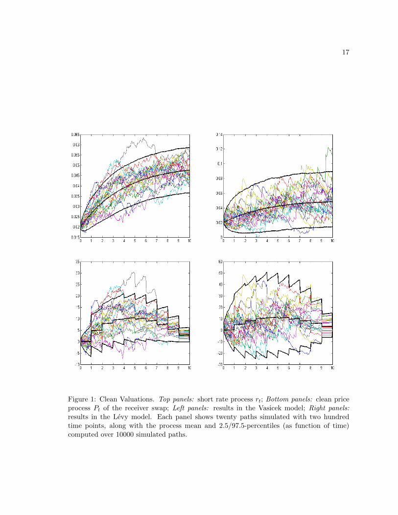
The top panels of Figure 1 show twenty paths, expectations and 2.5/97.5-percentilesover 10000 paths, simulated in the two models by an Euler scheme for the short-rate r on auniform time grid with two hundred time steps over [0, 10]yrs. Note that one does not seethe jumps on the right panel because we used interpolation between the points so that onecan identify better the twenty paths.

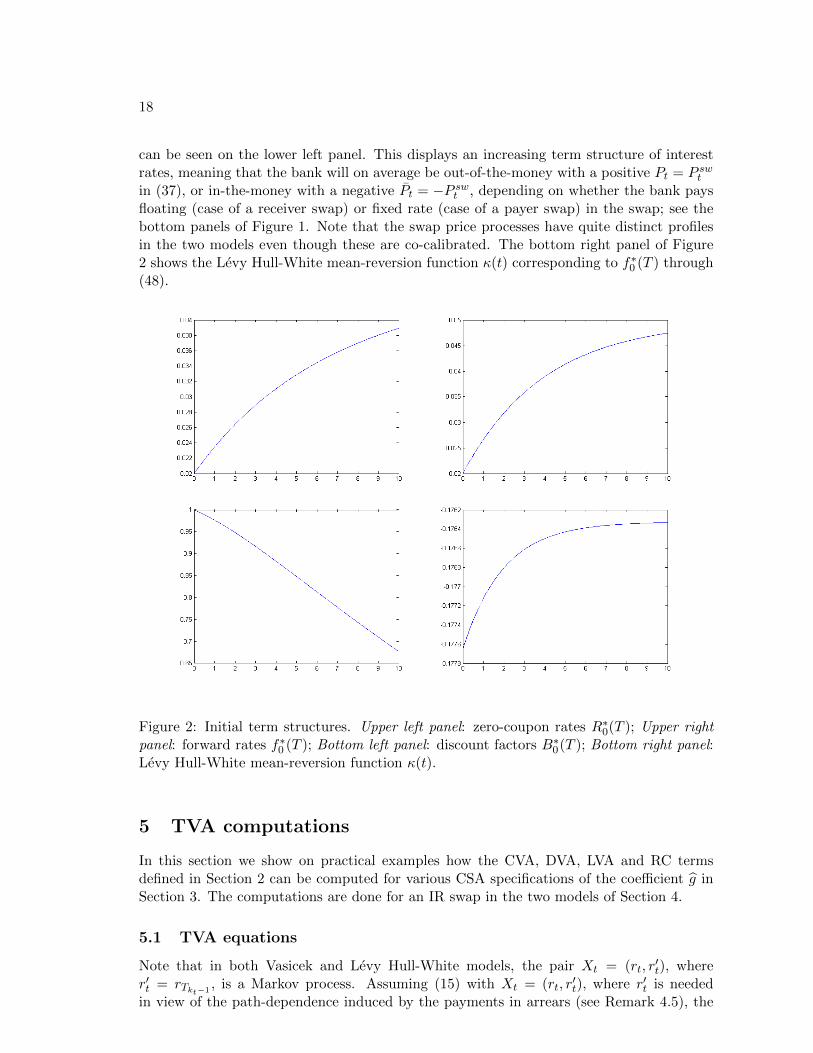
The top panels of Figure 2 show the initial zero-coupon rate term structure R∗0(T ) andthe corresponding forward curve f∗0 (T ), whilst the corresponding discount factors B∗0(T )

17

Figure 1: Clean Valuations. Top panels: short rate process rt; Bottom panels: clean priceprocess Pt of the receiver swap; Left panels: results in the Vasicek model; Right panels:results in the Levy model. Each panel shows twenty paths simulated with two hundredtime points, along with the process mean and 2.5/97.5-percentiles (as function of time)computed over 10000 simulated paths.

18

can be seen on the lower left panel. This displays an increasing term structure of interestrates, meaning that the bank will on average be out-of-the-money with a positive Pt = P swtin (37), or in-the-money with a negative Pt = −P swt , depending on whether the bank paysfloating (case of a receiver swap) or fixed rate (case of a payer swap) in the swap; see thebottom panels of Figure 1. Note that the swap price processes have quite distinct profilesin the two models even though these are co-calibrated. The bottom right panel of Figure2 shows the Levy Hull-White mean-reversion function κ(t) corresponding to f∗0 (T ) through(48).

Figure 2: Initial term structures. Upper left panel: zero-coupon rates R∗0(T ); Upper rightpanel: forward rates f∗0 (T ); Bottom left panel: discount factors B∗0(T ); Bottom right panel:Levy Hull-White mean-reversion function κ(t).

5 TVA computations

In this section we show on practical examples how the CVA, DVA, LVA and RC termsdefined in Section 2 can be computed for various CSA specifications of the coefficient g inSection 3. The computations are done for an IR swap in the two models of Section 4.

5.1 TVA equations

Note that in both Vasicek and Levy Hull-White models, the pair Xt = (rt, r′t), where

r′t = rTkt−1, is a Markov process. Assuming (15) with Xt = (rt, r

′t), where r′t is needed

in view of the path-dependence induced by the payments in arrears (see Remark 4.5), the

19

pre-default TVA Markovian BSDE in both models writes:

Θ(t,Xt) =Et(∫ T

tg(s,Xs, Θ(s,Xs))ds

), t ∈ [0, T ]. (58)

Even though finding deterministic solutions of the corresponding PDEs would be possiblein the above bivariate setups, in this paper we nevertheless favor BSDE schemes, as theyare more generic – in real-life higher-dimensional applications deterministic schemes cannotbe used anymore. We solve (58) by backward regression over the time-space grids generatedin Subsection 4.4; see the top panels of Figure 1. We thus approximate Θ(ω, t, ·) in (58) byΘji on the corresponding time-space grid, where the time-index i runs from 1 to n = 200

and the space-index j runs from 1 to m = 104. Denoting by Θi = (Θji )1≤j≤m the vector of

TVA values on the space grid at time i, we have Θn = 0, and then for every i = n−1, · · · , 0and j = 1, · · · ,m

Θji = Eji

(Θi+1 + gi+1

(t, Xi+1, Θi+1

)h)

for the time-step h = Tn = 0.05y (two weeks, roughly). The conditional expectations in

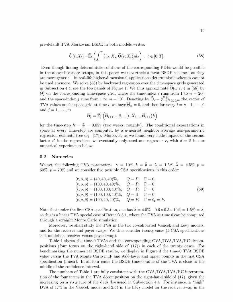
space at every time-step are computed by a d-nearest neighbor average non-parametricregression estimate (see e.g. [17]). Moreover, as we found very little impact of the secondfactor r′ in the regressions, we eventually only used one regressor r, with d = 5 in ournumerical experiments below.

5.2 Numerics

We set the following TVA parameters: γ = 10%, b = b = λ = 1.5%, λ = 4.5%, p =50%, p = 70% and we consider five possible CSA specifications in this order:

(r, ρ, ρ) = (40, 40, 40)%, Q = P, Γ = 0(r, ρ, ρ) = (100, 40, 40)%, Q = P, Γ = 0(r, ρ, ρ) = (100, 100, 40)%, Q = P, Γ = 0(r, ρ, ρ) = (100, 100, 40)%, Q = Π, Γ = 0(r, ρ, ρ) = (100, 40, 40)%, Q = P, Γ = Q = P.

(59)

Note that under the first CSA specification, one has λ = 4.5%−0.6×0.5×10% = 1.5% = λ,so this is a linear TVA special case of Remark 3.1, where the TVA at time 0 can be computedthrough a straight Monte Carlo simulation.

Moreover, we shall study the TVA in the two co-calibrated Vasicek and Levy models,and for the receiver and payer swaps. We thus consider twenty cases (5 CSA specifications× 2 models × receiver versus payer swap).

Table 1 shows the time-0 TVAs and the corresponding CVA/DVA/LVA/RC decom-positions (four terms on the right-hand side of (17)) in each of the twenty cases. Forbenchmarking the numerical BSDE results, we display in Figure 3 the time-0 TVA BSDEvalue versus the TVA Monte Carlo mid- and 95%-lower and upper bounds in the first CSAspecification (linear). In all four cases the BSDE time-0 value of the TVA is close to themiddle of the confidence interval.

The numbers of Table 1 are fully consistent with the CVA/DVA/LVA/RC interpreta-tion of the four terms in the TVA decomposition on the right-hand side of (17), given theincreasing term structure of the data discussed in Subsection 4.4. For instance, a “high”DVA of 1.75 in the Vasicek model and 2.34 in the Levy model for the receiver swap in the

20

Figure 3: BSDE values (in red) versus Monte Carlo mid-values and 95%-bounds (in blue)for the time-0 TVA in the linear CSA specification corresponding to the first line of (59).From left to right : receiver swap in the Vasicek model, receiver swap in the Levy model,payer swap in the Vasicek model, payer swap in the Levy model.

first row of Table 1 is consistent with the fact that with an increasing term structure of rates,the bank is on average out-of-the-money on the receiver swap with a positive Pt = P swt (seeFigure 1). The CVA, on the contrary, is moderate, as it should be for a receiver swap in anincreasing term structure of interest rates, and higher (“more negative”) in the Levy thanin the Vasicek model (-0.90 versus -0.06). The numbers of Table 1 are not negligible at allin view of the initial value of 100$ of the fixed leg of the swap (see [7], where significantdifferences in the valuation of swaps under various clearing conventions were also found).In particular, the LVA terms are quite significant in case of the payer swap with r and/orρ = 100%; see the corresponding terms in rows 3 and 4 in the two bottom parts of Ta-ble 1. The choice of r and ρ thus has tangible operational consequences, in regard of the“deal facilitating”(“deal hindering”) interpretation of the positive (negative) TVA terms asexplained at the end of Subsection 2.4. It is worthwhile noting that all this happens in asimplistic toy model of TVA, in which credit risk is independent from interest rates. Thesenumbers could be even much higher (in absolute value) in a model accounting for potentialwrong-way risk dependence effects between interest rates and credit risk; see Remark 4.1.

TVA CVA DVA LVA RC

1.47 -0.06 1.75 0.71 -0.92

1.40 -0.06 1.75 0.64 -0.91

0.40 -0.06 0.00 0.76 -0.29

0.66 -0.08 0.00 0.74 0.00

0.43 0.00 0.00 0.72 -0.29

TVA CVA DVA LVA RC

-1.90 -2.45 0.04 -0.68 1.17

-2.64 -2.45 0.04 -1.92 1.67

-2.67 -2.45 0.00 -1.92 1.68

-3.59 -1.77 0.00 -1.83 0.00

-0.50 0.00 0.00 -0.81 0.31

TVA CVA DVA LVA RC

1.34 -0.90 2.34 0.72 -0.85

0.93 -0.90 2.34 0.15 -0.68

-0.45 -0.90 0.00 0.32 0.12

-0.43 -0.76 0.00 0.32 0.00

0.44 0.00 0.00 0.72 -0.29

TVA CVA DVA LVA RC

-2.08 -3.28 0.64 -0.66 1.25

-3.17 -3.28 0.64 -2.41 1.92

-3.59 -3.28 0.00 -2.38 2.11

-4.80 -2.49 0.00 -2.26 0.00

-0.51 0.00 0.00 -0.81 0.31

Table 1: Time-0 TVAs and their decompositions into time-0 CVA, DVA, LVA and RC. Toptables: receiver swap; Bottom tables: payer swap; Left: Vasicek model; Right : Levy model.

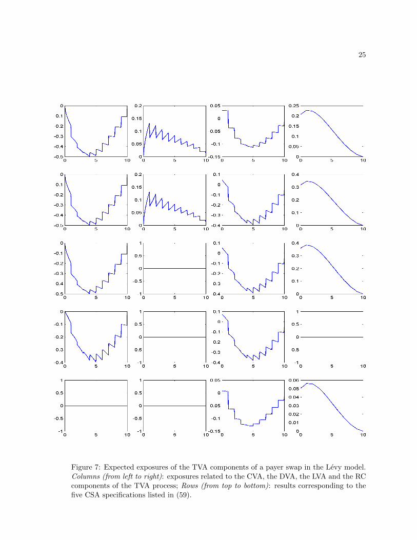
Figures 4 and 5 (receiver swap in the Vasicek and Levy model, respectively) and Figures6 and 7 (payer swap in the Vasicek and Levy model, respectively) show the “expected

21

exposures” of the four right-hand side terms of the “local” TVA decompositions (16) withϑ replaced by Θt therein. These exposures are computed as space-averages over 104 pathsas a function of time t. Each time-0 integrated term of the TVA in Table 1 correspondsto the surface under the corresponding curve in Figures 4 to 7 (with mappings between,respectively: Figure 4 and the upper left corner of Table 1, Figure 5 and the upper rightcorner of Table 1, Figure 6 and the lower left corner of Table 1, Figure 7 and the lower rightcorner of Table 1).

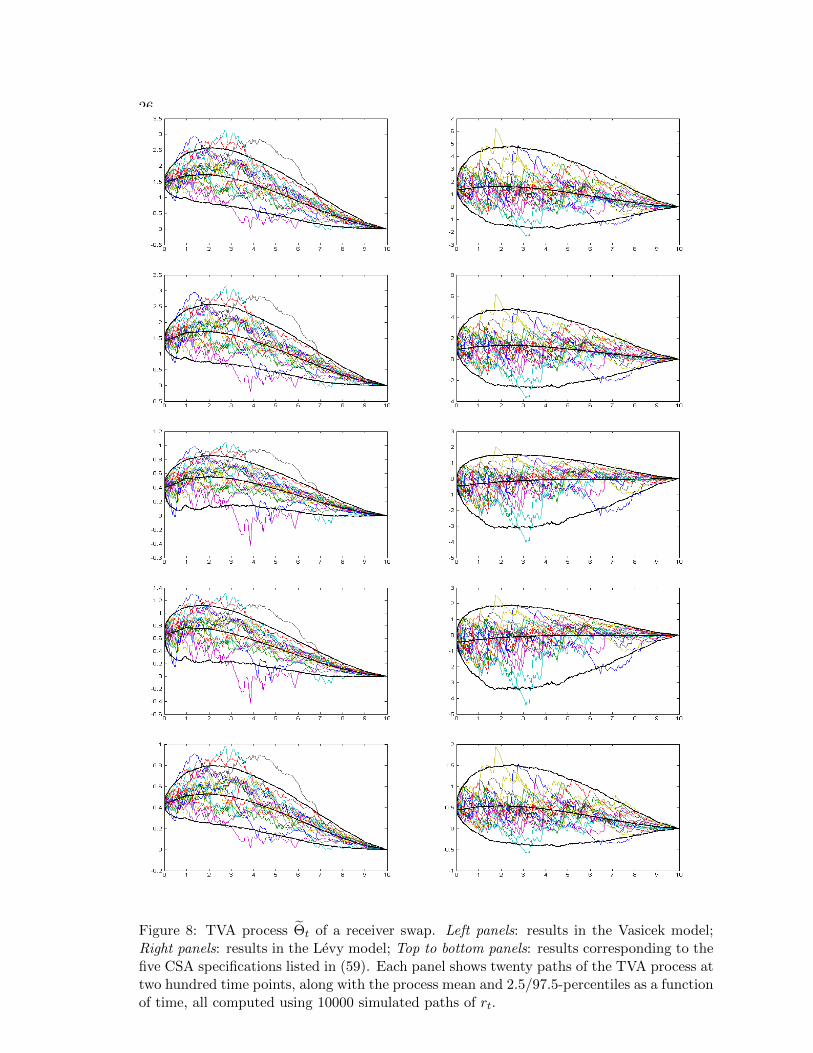
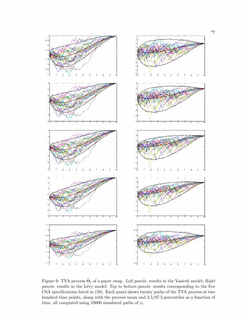
Finally, Figures 8 (receiver swap) and 9 (payer swap) show the TVA processes in thesame format as the swap clean prices at the bottom of Figure 1.

Conclusion

In this paper, which is a numerical companion to [9] and [10], we show on the standingexample of an interest rate swap how CVA, DVA, LVA and RC, the four “wings” (orpillars) of the TVA, can be (jointly) computed for various CSA and model specifications.Positive terms such as the DVA (resp. negative terms such as the CVA) can be consideredas “deal facilitating” (resp. “deal hindering”) as they increase (resp. decrease) the TVAand therefore decrease (resp. increase) the price (cost of the hedge) for the bank. Beliefsregarding the tangibility of a benefit-at-own-default, which depends in reality on the abilityto hedge and therefore monetize this benefit before the actual default, are controlled by thechoice of the “own recovery-rate” parameters ρ and r. Larger ρ and r mean smaller DVA andLVA and therefore smaller TVA, which in principle means less deals (or a recognition of ahigher cost of the deal). This is illustrated numerically in two alternative short rate modelsto emphasize the model-free feature of the numerical TVA computations through nonlinearregression BSDE schemes. The results show that the TVA model risk is under reasonablecontrol in the case of two co-calibrated models (models calibrated to the same initial termstructure, but also with the same level of volatility as imposed through calibration to capprices). We emphasize however that the latter observation applies to the “standard” casestudied in this paper without dominant wrong-way and gap risks, two important featureswhich will be dealt with in future work.

Acknowledgements

The research of S. Crepey and Z. Grbac benefited from the support of the ‘Chaire Risquede credit’, Federation Bancaire Francaise. R. Gerboud and N. Ngor are former studentsfrom the MSc quantitative finance program M2IF at Evry University. The authors warmlythank Anthony Dorme and Remi Takase, two other former M2IF students, for their help inthe numerical studies of the Levy model and of the TVA BSDEs.

References

[1] T. R. Bielecki, D. Brigo, and S. Crepey. Counterparty Risk Modeling – Collateralization,Funding and Hedging. CRC Press/Taylor & Francis, 2013. In preparation.

[2] D. Brigo, A. Capponi, A. Pallavicini, and V. Papatheodorou. Collateral margining inarbitrage-free counterparty valuation adjustment including re-hypotecation and nett-ing. Preprint, arXiv:0812.4064, 2011.

22

Figure 4: Expected exposures of the TVA components of a receiver swap in the Vasicekmodel. Columns (from left to right): exposures related to the CVA, the DVA, the LVA andthe RC components of the TVA process; Rows (from top to bottom): results correspondingto the five CSA specifications listed in (59).

23

Figure 5: Expected exposures of the TVA components of a receiver swap in the Levy model.Columns (from left to right): exposures related to the CVA, the DVA, the LVA and the RCcomponents of the TVA process; Rows (from top to bottom): results corresponding to thefive CSA specifications listed in (59).

24

Figure 6: Expected exposures of the TVA components of a payer swap in the Vasicek model.Columns (from left to right): exposures related to the CVA, the DVA, the LVA and the RCcomponents of the TVA process; Rows (from top to bottom): results corresponding to thefive CSA specifications listed in (59).

25

Figure 7: Expected exposures of the TVA components of a payer swap in the Levy model.Columns (from left to right): exposures related to the CVA, the DVA, the LVA and the RCcomponents of the TVA process; Rows (from top to bottom): results corresponding to thefive CSA specifications listed in (59).

26

Figure 8: TVA process Θt of a receiver swap. Left panels: results in the Vasicek model;Right panels: results in the Levy model; Top to bottom panels: results corresponding to thefive CSA specifications listed in (59). Each panel shows twenty paths of the TVA process attwo hundred time points, along with the process mean and 2.5/97.5-percentiles as a functionof time, all computed using 10000 simulated paths of rt.

27

Figure 9: TVA process Θt of a payer swap. Left panels: results in the Vasicek model; Rightpanels: results in the Levy model; Top to bottom panels: results corresponding to the fiveCSA specifications listed in (59). Each panel shows twenty paths of the TVA process at twohundred time points, along with the process mean and 2.5/97.5-percentiles as a function oftime, all computed using 10000 simulated paths of rt.

28

[3] D. Brigo, M. Morini, and A. Pallavicini. Counterparty Credit Risk, Collateral andFunding with Pricing Cases for All Asset Classes. Wiley Finance, 2013. Forthcoming.

[4] D. Brigo and A. Pallavicini. Counterparty risk and contingent CDS under correlationbetween interest-rates and default. Risk Magazine, pages 84–88, February 2008.

[5] C. Burgard and M. Kjaer. PDE representations of options with bilateral counterpartyrisk and funding costs. The Journal of Credit Risk, 7(3):1–19, 2011.

[6] G. Cesari, J. Aquilina, N. Charpillon, Z. Filipovic, G. Lee, and I. Manda. Modelling,Pricing, and Hedging Counterparty Credit Exposure. Springer Finance, 2010.

[7] R. Cont, Radu Mondescu, and Yuhua Yu. Central clearing of interest rate swaps: Acomparison of offerings. SSRN eLibrary, 2011.

[8] S. Crepey. Wrong-way and gap risks modeling: A marked default time approach. Inpreparation, 2012.

[9] S. Crepey. Bilateral Counterparty risk under funding constraints – Part I: Pricing.Mathematical Finance, January 2013. Online First.

[10] S. Crepey. Bilateral Counterparty risk under funding constraints – Part II: CVA.Mathematical Finance, January 2013. Online First.

[11] S. Crepey and R. Douady. The whys of the LOIS: credit skew and funding spreadvolatility. Risk Magazine, 2013. Forthcoming.

[12] S. Crepey, Z. Grbac, and H. N. Nguyen. A multiple-curve HJM model of interbankrisk. Mathematics and Financial Economics, 6 (3):155–190, 2012.

[13] N. El Karoui, S. Peng, and M.-C. Quenez. Backward stochastic differential equationsin finance. Mathematical Finance, 7:1–71, 1997.

[14] D. Filipovic and Anders B. Trolle. The term structure of interbank risk. Journal ofFinancial Economics, 2012. Forthcoming.

[15] M. Fujii, Y. Shimada, and A. Takahashi. Collateral posting and choice of collateralcurrency. SSRN eLibrary, 2010.

[16] M. Fujii and A. Takahashi. Derivative pricing under asymmetric and imperfect collat-eralization and CVA. SSRN eLibrary, 2011.

[17] T. Hastie, R Tibshirani, and J. Friedman. The Elements of Statistical Learning: DataMining, Inference, and Prediction. Springer, 2009.

[18] P. Henry-Labordere. Cutting CVA’s complexity. Risk Magazine, pages 67–73, July2012.

[19] M. Musiela and M. Rutkowski. Martingale Methods in Financial Modelling. Springer,2nd edition, 2005.

[20] V. Piterbarg. Cooking with collateral. Risk Magazine, pages 58–63, July 2012.

[21] B. De Prisco and D. Rosen. Modelling stochastic counterparty credit exposures forderivatives portfolios. In M. Pykhtin, editor, Counterparty Credit Risk Modelling:Risk Management, Pricing and Regulation. RISK Books, London, 2005.