coulomb branch hilbert series and three dimensional ... · coulomb branch hilbert series and three...
TRANSCRIPT
CERN-PH-TH/2014-036
IMPERIAL-TP-14-SC-02
Coulomb branch Hilbert series
and Three Dimensional Sicilian Theories
Stefano Cremonesi,a Amihay Hanany,a Noppadol Mekareeya,b
and Alberto Zaffaronic,d
aTheoretical Physics Group, Imperial College London,
Prince Consort Road, London, SW7 2AZ, UKbTheory Division, Physics Department, CERN,
CH-1211, Geneva 23, SwitzerlandcDipartimento di Fisica, Universita di Milano-Bicocca,
I-20126 Milano, ItalydINFN, sezione di Milano-Bicocca, I-20126 Milano, Italy
E-mail: [email protected], [email protected],
[email protected], [email protected]
Abstract: We evaluate the Coulomb branch Hilbert series of mirrors of three di-
mensional Sicilian theories, which arise from compactifying the 6d (2, 0) theory with
symmetry G on a circle times a Riemann surface with punctures. We obtain our result
by gluing together the Hilbert series for building blocks Tρ(G), where ρ is a certain
partition related to the dual group of G, which we evaluated in a previous paper.
The result is expressed in terms of a class of symmetric functions, the Hall-Littlewood
polynomials. As expected from mirror symmetry, our results agree at genus zero with
the superconformal index prediction for the Higgs branch Hilbert series of the Sicilian
theories and extend it to higher genus. In the A1 case at genus zero, we also evaluate
the Coulomb branch Hilbert series of the Sicilian theory itself, showing that it only
depends on the number of external legs.
arX
iv:1
403.
2384
v2 [
hep-
th]
23
Sep
2014
Contents
1 Introduction 1
2 Coulomb branch Hilbert series of a 3d N = 4 gauge theory 3
2.1 The monopole formula 4
2.2 The Hall-Littlewood formula 6
2.2.1 Tρ(SU(N)) 6
2.2.2 Tρ(G∨) 8
3 Mirrors of 3d Sicilian theories of A-type 10
3.1 Mirrors of tri-vertex theories: star-shaped U(2)× U(1)e/U(1) quivers 11
3.1.1 Computation of the Hilbert series for general g and e 14
3.2 The Coulomb branch of the mirror of TN 15
3.3 The Coulomb branch of the mirror of a general 3d Sicilian theory 18
3.3.1 The case of genus zero 19
3.3.2 Mirror of the SU(3) Sicilian theory with g = 1 and a maximal
puncture 20
4 Mirrors of 3d Sicilian theories of D-type 22
4.1 D3 punctures 23
4.1.1 D3 punctures: (32), (16) and (16) 24
4.2 D4 punctures 25
4.2.1 D4 punctures: (5, 3), (22, 14) and (18) 26
4.2.2 D4 punctures: (32, 12), (22, 14) and (22, 14) 27
4.2.3 D4 punctures: (5, 3), (5, 3), (24) and (3, 15) 28
5 Coulomb branch Hilbert series of 3d theories with tri-vertices 30
5.1 The case of g = 0 31
5.1.1 General formula for g = 0 and any e 31
5.1.2 Special case of g = 0 and e = 6 32
5.2 Turning on background fluxes 33
5.3 Generating functions of Coulomb branch Hilbert series 33
5.3.1 Gluing generating functions and recursive formula 34
5.3.2 Proof of the symmetry of the generating functions Ge(z) 36
6 Conclusion 38
– i –
A Mirrors of Sicilian theories with twisted D punctures 39
A.1 The Coulomb branch Hilbert series of mirror theories 41
A.1.1 Twisted punctures (2, 14), (2, 14) and untwisted puncture (4, 4) 42
A.1.2 Twisted punctures (6), (16) and untwisted puncture (18) 43
A.1.3 Four SO(4) twisted punctures: (2), (2), (12), (12) 44
1 Introduction
A general formula for computing the generating function (Hilbert series) for the chiral
ring associated with the Coulomb branch of three dimensional N = 4 gauge theories
has been recently proposed [1]. The formula counts monopole operators dressed by
classical operators and includes quantum corrections. It can be applied to any 3d
N = 4 supersymmetric gauge theories that possess a Lagrangian description and that
are good or ugly in the sense of [2]. The formula has been successfully tested against
mirror symmetry in many cases [1, 3].
In a companion paper we developed a machinery for computing Coulomb branch
Hilbert series for wide classes of N = 4 gauge theories by using gluing techniques.
We computed the Coulomb branch Hilbert series with background fluxes for the flavor
symmetry of the three dimensional superconformal field theories known as Tρ(G) [2], a
class of linear quiver theories with non-decreasing ranks associated with a partition ρ
and a flavor symmetry G. We found an intriguing connection with a class of symmetric
functions, the Hall-Littlewood polynomials, which have also appeared in the recent
literature in the context of the superconformal index of four dimensionalN = 2 theories
[4]. We clarify the meaning of this connection in the following. The Tρ(G) theories
serve as basic building blocks for constructing more complicated theories.
In this paper we consider the theories that arise from compactifying the 6d (2, 0)
theory with symmetry G = SU(N), SO(2N) on a circle times a Riemann surface with
punctures. These are known as three dimensional Sicilian theories. With the excep-
tion of the SU(2) case, they have no Lagrangian description [5]. We are interested in
their mirror which can be obtained as follows. Starting from a set of building blocks
{Tρ1(G), Tρ2(G), . . . , Tρn(G)}, one can construct a new theory by gauging the common
centerless flavor symmetry G/Z(G), where Z(G) is the center of G. We refer to this
procedure as ‘gluing’ the building blocks together. The resulting theory is the afore-
mentioned mirror of the theory associated to a sphere with punctures {ρ1,ρ2, . . . ,ρn}[6, 7].
– 1 –
The main purpose of this paper is to compute the Coulomb branch Hilbert series
of these mirrors. We do this by gluing together the Hilbert series of the theories
Tρi(G) as explained in [3]. By mirror symmetry, our results should agree with the
Higgs branch Hilbert series of the Sicilian theories. The latter can be computed for
the four dimensional version of the theory, since the Higgs branch of a theory with
eight supercharges is protected against quantum corrections by a non-renormalization
theorem [8] and therefore is the same in all dimensions. Although the theory is non-
Lagrangian, at genus zero the Higgs branch Hilbert series can be written in terms of the
Hall-Littlewood indices proposed in [4, 9]. We find perfect agreement with the results
in [4, 9, 10], as predicted by mirror symmetry.
Our result clarifies why the Hall-Littlewood polynomials appear in two different
contexts, the Coulomb branch Hilbert series for the Tρ(G) theories and a limit of
the four dimensional superconformal index of Sicilian theories. It is interesting to
observe how the structure of the superconformal index formula (see for example (3.31)),
obtained in a completely different manner, can be naturally reinterpreted in terms of
gluing of three dimensional building blocks.
Our gluing formula easily extends to punctured Riemann surfaces of higher genus,
by incorporating adjoint hypermultiplets in the mirror theory [6]. For such Riemann
surfaces the Hall-Littlewood index of the 4d non-Lagrangian theory differs from the
Higgs branch Hilbert series, as discussed in [4]. Our formula for the Coulomb branch
Hilbert series of the 3d Lagrangian mirror theory (3.30) provides the Higgs branch
Hilbert series of the (3d or 4d) non-Lagrangian Sicilian theory, for any genus g, as long
as the theory is not bad in the sense of [2]. In section 3.1, we successfully test our
higher genus prediction for the case of A1 Sicilian theories, also known as tri-vertex
theories. These are 3d N = 4 Lagrangian theories associated to a graph with tri-valent
vertices, where a finite line denotes an SU(2) gauge group, an infinite line denotes
an SU(2) global symmetry, and a vertex denotes 8 half-hypermultiplets in the tri-
fundamental representation of SU(2)3. These graphs are characterized by the genus g
and the number of external legs e. The Higgs branch Hilbert series of such theories were
computed directly in [11]. In section 3.1.1 we reproduce that result from the Coulomb
branch of the mirror theory.
As an addition to the main line of this paper, which focusses on the Coulomb branch
of mirrors of three dimensional Sicilian theories, in section 5 we study the Coulomb
branch of tri-vertex theories themselves at genus zero using the monopole formula. We
find that the Coulomb branch Hilbert series depends only on e and not on the details
of the graph, as suggested in [6].
The paper is organized as follows. In section 2 we review the formula for the
Coulomb branch Hilbert series of N = 4 theories, the gluing technique and the Hall-
– 2 –
Littlewood formula for the Tρ(G) theories. In section 3 we compute the Coulomb
branch Hilbert series of the mirrors of three dimensional Sicilian theories with A-type
punctures at arbitrary genus g. We examine in particular the case of the TN theory. We
successfully compare the result for genus zero with the superconformal index prediction
for Higgs branch Hilbert series of the Sicilian theories given in [4, 9]. We also give
explicit examples for theories at higher genus. In the SU(2) case, where the Sicilian
theories are Lagrangian, we compare our result with the Higgs branch Hilbert series
computed in [11] finding perfect agreement. In section 4 we extend the analysis to
theories of type D. As a general check of our predictions, we demonstrate the equivalence
between D3 and A3 punctures and we compute the Coulomb branch Hilbert series for a
set of D4 punctures where the Higgs branch Hilbert series can be explicitly evaluated,
finding perfect agreement. In section 5 we compute the Hilbert series of the tri-vertex
theories at genus zero showing that they only depend on the number of external legs. In
section 5.3 we present generating functions and recursive formulae, which are powerful
tools for computing the Hilbert series of tri-vertex theories. Finally, in appendix A we
consider theories of type D with twisted punctures.
Note added: One might ask whether there is any relation between the Coulomb
branch Hilbert series that we study and the 3d superconformal index [12–14]. Indeed,
a recent work [15] appeared after the submission of this paper, showing that the su-
perconformal index of a 3d N = 4 theory reduces to the Hilbert series in a particular
limit.
2 Coulomb branch Hilbert series of a 3d N = 4 gauge theory
Our main aim is to study the Coulomb branch of three dimensional N = 4 gauge
theories. Classically, this branch is parameterized by the vacuum expectation values
of the triplet of scalars in the N = 4 vector multiplets and by the vacuum expectation
value of the dual photons, at a generic point where the gauge group is spontaneously
broken to its maximal torus. This yields a HyperKahler space of quaternionic dimension
equal to the rank of the gauge group. The Coulomb branch is, however, not protected
against quantum corrections and the associated chiral ring has a complicated structure
involving monopole operators in addition to the classical fields in the Lagrangian.
A suitable quantum description of the chiral ring on the Coulomb branch is to
replace the above description by monopole operators. The gauge invariant BPS objects
on the branch are monopole operators dressed by a product of a certain scalar field in
the vector multiplet. The spectrum of such BPS objects can be studied in a systematic
way by computing their partition function, known as the Hilbert series. A Hilbert
– 3 –

series is a generating function of the chiral ring, which enumerates gauge invariant
BPS operators which have a non-zero expectation value along the Coulomb branch. As
extensively discussed in [1, 3], a general formula for the Hilbert series of the Coulomb
branch of an N = 4 theory can be computed based on this principle. We refer to such
a formula as the monopole formula.
In [3] we found an analytic expression for the Coulomb branch Hilbert series of
a class of theories called Tρ(G) [2], where G is a classical group and ρ is a partition
associated with the GNO dual group G∨. Such a theory has a Lagrangian description
[2, 3, 6]. The Hilbert series of these theories can be conveniently written in terms of
Hall-Littlewood polynomials [3], and the corresponding formula is dubbed the Hall-
Littlewood formula. In the following section we show that the Hall-Littlewood formula
is a convenient tool to compute the Coulomb branch Hilbert series of mirrors of three
dimensional Sicilian theories.
Let us now summarize important information on the monopole and Hall-Littlewood
formulae for Coulomb branch Hilbert series.
2.1 The monopole formula
The monopole formula [1] counts all gauge invariant chiral operators that can acquire
a non-zero expectation value along the Coulomb branch, according to their dimension
and quantum numbers. The operators are written in an N = 2 formulation and the
N = 4 vector multiplet is decomposed into an N = 2 vector multiplet and a chiral
multiplet Φ transforming in the adjoint representation of the gauge group. We refer to
[1] for an explanation of the formula and simply quote the final result here.
The formula for a good or ugly [2] theory with gauge group G reads
HG(t, z) =∑
m∈ΓG∨/WG∨
zJ(m)t∆(m)PG(t;m) . (2.1)
The sum is over the magnetic charges of the monopoles m which, up to a gauge trans-
formation, belong to a Weyl Chamber of the weight lattice ΓG∨ of the GNO dual group
[16]. PG(t;m) is a factor which counts the gauge invariants of the gauge group Hmunbroken by the monopole m made with the adjoint scalar field φ in the multiplet Φ,
according to their dimension. It is given by
PG(t;m) =r∏i=1
1
1− tdi(m), (2.2)
– 4 –

where di(m), i = 1, . . . , rank Hm are the degrees of the independent Casimir invariants
of Hm. ∆(m) is the quantum dimension of the monopole which is given by [2, 17–19]
∆(m) = −∑
α∈∆+(G)
|α(m)|+ 1
2
n∑i=1
∑ρi∈Ri
|ρi(m)| , (2.3)
where α are the positive roots of G and ρi ∈ Ri the weights of the matter field
representation Ri under the gauge group. z is a fugacity valued in the topological
symmetry group, which exists if G is not simply connected, and J(m) the topological
charge of a monopole operator of GNO charges m.
Turning on background magnetic fluxes. As discussed in [3], the formula can
be generalized to include background monopole fluxes for a global flavor symmetry GF
acting on the matter fields:
HG,GF (t,mF , z) =∑
m∈ΓG∨/WG∨
zJ(m)t∆(m,mF )PG(t;m) . (2.4)
The sum is only over the magnetic fluxes of the gauge group G but depends on the
weights mF of the dual group G∨F which enter explicitly in the dimension formula (2.3)
through all the matter fields that are charged under the global symmetry GF . By using
the global symmetry we can restrict the value of mF to a Weyl chamber of G∨F and
take mF ∈ ΓG∨F /WG∨F.
The gluing technique. We can construct more complicated theories by starting
with a collection of theories and gauging some common global symmetry GF they
share. The Hilbert series of the final theory where GF is gauged is given by multiplying
the Hilbert series with background fluxes for GF of the building blocks, summing over
the monopoles of GF and including the contribution to the dimension formula of the
N = 4 dynamical vector multiplets associated with the gauged group GF :
H(t) =∑
mF ∈ΓG∨F/WG∨
F
t−
∑αF∈∆+(GF ) |αF (mF )|
PGF (t;mF )∏i
H(i)G,GF
(t,mF ) , (2.5)
where αF are the positive roots of GF and the product with the index i runs over the
Hilbert series of the i-th theory that is taken into the gluing procedure. Since we can
always make αF (mF ) non-negative by choosing mF in the main Weyl chamber, the
evaluation of H(t) turns out to have no absolute values. The formula (2.5) can be
immediately generalized to include fugacities for the topological symmetries acting on
the Coulomb branch.
– 5 –

In the next sections we will provide explicit and general formulae for many in-
teresting 3d N = 4 superconformal theories including mirrors of M5-brane theories
compactified on a circle times a Riemann surfaces with punctures. They are obtained
by gluing a simple class of building blocks that we now discuss.
2.2 The Hall-Littlewood formula
As extensively discussed in [3], the Coulomb branch Hilbert series of Tρ(G∨) for a clas-
sical group G can be computed using formulae involving Hall-Littlewood polynomials.
The main purpose of this paper is to show that these formulae are useful for comput-
ing Coulomb branch Hilbert series of mirrors of 3d Sicilian theories. For the sake of
completeness of the paper, we review Hall-Littlewood formulae below. We first present
the formula for G = SU(N) and then discuss the formula for other classical groups,
namely SO(N) and USp(2N).
2.2.1 Tρ(SU(N))
The quiver diagram for Tρ(SU(N)) is
[U(N)]− (U(N1))− (U(N2))− · · · − (U(Nd)), (2.6)
where the partition ρ of N is given by
ρ = (N −N1, N1 −N2, N2 −N3, . . . , Nd−1 −Nd, Nd) , (2.7)
with the restriction that ρ is a non-increasing sequence:
N −N1 ≥ N1 −N2 ≥ N2 −N3 ≥ · · · ≥ Nd−1 −Nd ≥ Nd > 0 . (2.8)
The quiver theory in (2.6) can be realised from brane configurations as proposed in
[20].
The Coulomb branch Hilbert series of this theory can be written as
H[Tρ(SU(N))](t;x1, . . . , xd+1;n1, . . . , nN)
= t12δU(N)(n)(1− t)NKU(N)
ρ (x; t)ΨnU(N)(xt
12wρ ; t) ,
(2.9)
where the Hall-Littlewood polynomial associated with the group U(N) is given by
ΨnU(N)(x1, . . . , xN ; t) =
∑σ∈SN
xn1
σ(1) . . . xnNσ(N)
∏1≤i<j≤N
1− tx−1σ(i)xσ(j)
1− x−1σ(i)xσ(j)
, (2.10)
with n1, . . . , nN the background GNO charges for U(N) group, with
n1 ≥ n2 ≥ · · · ≥ nN ≥ 0 . (2.11)
– 6 –
The notation δU(N) denotes the sum over positive roots of the group U(N) acting on
the background charges ni:
δU(N)(n) =∑
1≤i<j≤N
(ni − nj) =N∑j=1
(N + 1− 2j)nj . (2.12)
The fugacities x1, . . . , xd+1 are subject to the following constraint which fixes the overall
U(1):
d+1∏i=1
xρii = 1 . (2.13)
The vector wr denotes the weights of the SU(2) representation of dimension r:
wr = (r − 1, r − 3, . . . , 3− r, 1− r) . (2.14)
Hence the notation t12wr represents the vector
t12wr = (t
12
(r−1), t12
(r−3), . . . , t−12
(r−3), t−12
(r−1)) . (2.15)
In (2.9) and henceforth, we abbreviate
ΨnU(N)(xt
12wρ ; t) := Ψ
(n1,...,nN )U(N) (x1t
12wρ1 , x2t
12wρ2 , . . . , xd+1t
12wρd+1 ; t) . (2.16)
The prefactor KU(N)ρ (x; t) is given by
KU(N)ρ (x; t) =
length(ρT )∏i=1
ρTi∏j,k=1
1
1− aijaik, (2.17)
where ρT denotes the transpose of the partition ρ and we associate the factors
aij = xj t12
(ρj−i+1) , i = 1, . . . , ρj
aik = x−1k t
12
(ρk−i+1) , i = 1, . . . , ρk(2.18)
to each box in the Young tableau. The powers of t inside aij and aik are positive by
construction.
We demonstrate the HL formula (2.9) in a number of examples in section 3.
– 7 –

2.2.2 Tρ(G∨)
In this section we review a generalized version of formula (2.9) to a more general
classical group G. The quiver diagrams are explicitly given in [3]. Further discussions
regarding mathematical aspects of this formula can be found in [3, 21, 22].
The partition ρ induces an embedding ρ : Lie(SU(2))→ Lie(G) such that
[1, 0, . . . , 0]G =⊕i
[ρi − 1]SU(2) . (2.19)
The global symmetry Gρ associated to the puncture ρ = [ρi], with rk the number of
times that part k appears in the partition ρ, is given by
Gρ =
S (∏
k U(rk)) G = U(N) ,∏k odd SO(rk)×
∏k even USp(rk) G = SO(2N + 1) or SO(2N) ,∏
k odd USp(rk)×∏
k even SO(rk) G = USp(2N) .
(2.20)
Let x1, x2, . . . be fugacities for the global symmetry Gρ, the commutant of ρ(SU(2))
in G, and r(G) the rank of G. In [3] we have conjectured that the Coulomb branch
Hilbert series is given by the HL formula
H[Tρ(G∨)](t;x;n1, . . . , nr(G)) = t
12δG∨ (n)(1− t)r(G)KG
ρ (x; t)ΨnG(a(t,x); t) . (2.21)
Here ΨnG is the Hall-Littlewood polynomial associated to a Lie group G, given by
ΨnG(x1, . . . , xr; t) =
∑w∈WG
xw(n)∏
α∈∆+(G)
1− tx−w(α)
1− x−w(α), (2.22)
where WG denotes the Weyl group of G, ∆+(G) the set of positive roots of G, n =∑ri=1 niei, with {e1, . . . , er} the standard basis of the weight lattice and r the rank of
G. See Appendix B of [3] for more details. G∨ is the GNO dual group [16]. The power
δG∨(n) is the sum over positive roots α ∈ ∆+(G∨) of the flavor group G∨ acting on
the background monopole charges n:
δG∨(n) =∑
α∈∆+(G∨)
|α(n)| . (2.23)
Explicitly, for classical groups G and fluxes n in the fundamental Weyl chamber, these
are given by
δG∨(n) =
∑Nj=1(N + 1− 2j)nj G∨ = G = U(N),∑Nj=1(2N + 1− 2j)nj G∨ = BN , G = CN∑Nj=1(2N + 2− 2j)nj G∨ = CN , G = BN∑N−1j=1 (2N − 2j)nj G∨ = G = DN .
(2.24)
– 8 –
The argument a(t,x) of the HL polynomial, which we shall henceforth abbreviate
as a, is determined by the following decomposition of the fundamental representation
of G to Gρ × ρ(SU(2)):
χGfund(a) =∑k
χGρkfund(xk)χ
SU(2)[ρk−1](t
1/2) , (2.25)
where Gρk denotes a subgroup of Gρ corresponding to the part k of the partition ρ that
appears rk times. Formula (2.25) determines a as a function of t and {xk} as required.
Of course, there are many possible choices for a; the choices that are related to each
other by outer-automorphisms of G are equivalent.
The prefactor KGρ (x; t) is independent of n and can be determined as follows. The
embedding specified by ρ induces the decomposition
χGAdj(a) =∑
j=0, 12,1, 3
2,...
χGρRj
(xj)χSU(2)[2j] (t1/2) , (2.26)
where a on the left hand side is the same a as in (2.25). Each term in the previous
formula gives rise to a plethystic exponential,1 giving
KGρ (x; t) = PE
∑j=0, 1
2,1, 3
2,...
tj+1χGρRj
(xj)
. (2.27)
As a remark, in the special case when ρ : Lie(SU(2)) → Lie(G) is a principal
embedding ρprinc (see, e.g. [22]), the global symmetry acting on the Coulomb branch
is trivial Gρprinc = 1, the prefactor KGρprinc
(t) = PG(t; 0) equals the Casimir factor of G
(or equivalently G∨), and the Hall-Littlewood formula (2.21) reduces to
H[Tρprinc(G∨)](t;n1, . . . , nr(G)) = 1 . (2.28)
This identity has a simple physical interpretation in the context of mirrors of Sicilian
theories that we consider in this paper: adding an empty puncture does not affect the
Hilbert series of the Sicilian theory.
In the following we discuss several examples of mirrors of 3d Sicilian theories for
which we use the Hall-Littlewood formulae to compute their Coulomb branch Hilbert
series.
1See Appendix A of [1] for the definition.
– 9 –

3 Mirrors of 3d Sicilian theories of A-type
In this and the next section we evaluate the Coulomb branch Hilbert series of the
mirror of the theories arising from compactifying the 6d (2, 0) theory with symmetry G
on a circle times a Riemann surface with punctures, also called Sicilian theories. These
theories and their Coulomb branch Hilbert series will be obtained by gluing together
Tρ(G) building blocks.
Given a set of theories {Tρ1(G), . . . , Tρn(G)}, we can construct a new theory by
gauging the common centerless flavor symmetry G/Z(G); see Figure 1.2 The resulting
theory is the mirror of the theory on M5-branes wrapping a circle times a Riemann
sphere with punctures ρ1, . . . ,ρn [6, 7]. For example, taking G = SU(3) and ρ1 =
ρ2 = ρ3 = (1, 1, 1) we obtain a mirror of the T3 theory reduced to three dimensions.
Recall that the Higgs branch of the 3d T3 theory is the reduced moduli space of 1 E6
instantons on C2 and the Coulomb branch is C2/E6. The moduli spaces of k E6, E7
and E8 instantons on C2 can be also realized as the Higgs branch of the 6d (2, 0) theory
compactified on a circle times a Riemann sphere with punctures.
G/Z(G)
Tρ1(G)
Tρ2 (G)
Tρ3 (G)
Tρn(G)
Tρn-1 (G)
Figure 1. Gluing Tρ1(G), . . . , Tρn(G) via the common centerless flavor symmetry G/Z(G).
This is a mirror theory of the theory on M5-brane compactified on a circle times a Riemann
sphere with punctures ρ1, . . . ,ρn.
2For G = U(N), this also involves factoring out a decoupled U(1) gauge group.
– 10 –
We demonstrate how to ‘glue’ the Hilbert series Tρn(G) together to obtain the
Coulomb branch Hilbert series of the mirror of the theory on M5-branes compactified
on S1 times a Riemann sphere with punctures {ρi}. By mirror symmetry, this is
equal to the Higgs branch Hilbert series of the latter. The theories on M5-branes are
not Lagrangian, but, when the genus of the Riemann surface is zero, the Higgs branch
Hilbert series can be evaluated by the Hall-Littlewood (HL) limit of the superconformal
index [4]. We find perfect agreement with the results in [4], which were obtained in a
completely different manner. Upon introduction of g G-adjoint hypermultiplets [6], our
formulae can be used also for genus greater than one, where the Higgs branch Hilbert
series for the M5-brane theories cannot be evaluated as a limit of the 4d superconformal
index.3 In section 3.1 we will be able to test the validity of our result for higher genus in
the case of two M5 branes where the theory is Lagrangian and we can use conventional
methods for computing the Higgs branch Hilbert series.
In this section we discuss the case of A-type theories with G = SU(N) and in the
next section we discuss D-type theories with G = SO(2N).
3.1 Mirrors of tri-vertex theories: star-shaped U(2)× U(1)e/U(1) quivers
We start by considering the Coulomb branch Hilbert series of the mirrors of theories on
two M5-branes compactified on a circle times a Riemann surface with punctures. The
latter are referred to as 3d SU(2) Sicilian theories [6, 23] or 3d theories with tri-vertices
[11]. They are Lagrangian theories whose quiver is explicitly discussed in section 5.
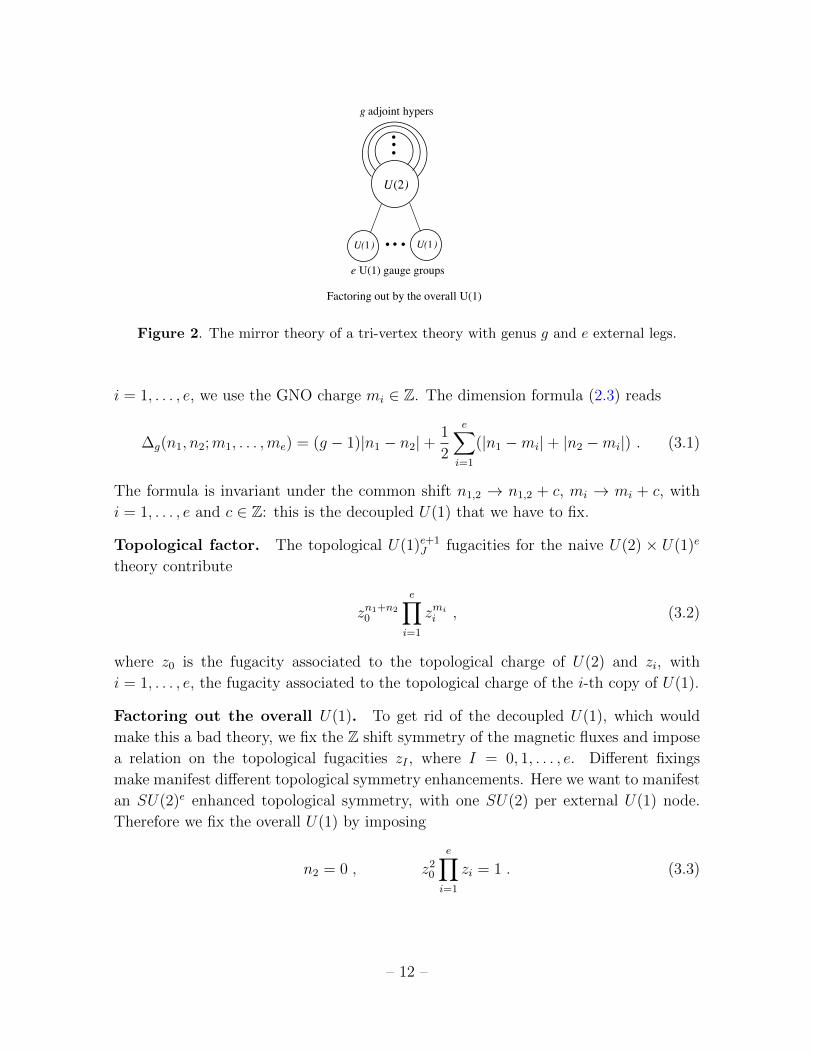
According to [6], the mirror of a tri-vertex theory with genus g and e external legs is a
star-shaped U(2)×U(1)e/U(1) quiver gauge theory with the U(2) node with g adjoint
hypermultiplets in the center, attached to e ≥ 3 U(1) nodes around it. The quiver is
depicted in Figure 2.
The overall U(1) gauge group in the quiver is decoupled and needs to be factored
out. It is crucial to mod out by the overall U(1) properly: in particular the quiver
with an SU(2) node in the center, attached to e U(1) nodes around it, gives the wrong
Coulomb branch, which disagrees with the Higgs branch of the g = 0 tri-vertex theory
with e ≥ 3 legs [11]. The reason is that U(2) = U(1)× SU(2)/Z2.
Let us first consider the U(2) × U(1)e quiver gauge theory which includes the
decoupled overall U(1). We use GNO charges n1 and n2 for U(2), related to the integer
weights n1 ≥ n2 > −∞ in the Weyl chamber. For the i-th U(1) gauge group, with
3For genus greater than 1, the F-terms of the theory are not all independent. As a result, the HL
limit of the 4d superconformal index fails to reproduce the Higgs branch Hilbert series. For a very
clear explanation of this technical fact, see section 5 of [4].
– 11 –
U(2)
U(1)U(1)
g adjoint hypers
e U(1) gauge groups
Factoring out by the overall U(1)
Figure 2. The mirror theory of a tri-vertex theory with genus g and e external legs.
i = 1, . . . , e, we use the GNO charge mi ∈ Z. The dimension formula (2.3) reads
∆g(n1, n2;m1, . . . ,me) = (g − 1)|n1 − n2|+1
2
e∑i=1
(|n1 −mi|+ |n2 −mi|) . (3.1)
The formula is invariant under the common shift n1,2 → n1,2 + c, mi → mi + c, with
i = 1, . . . , e and c ∈ Z: this is the decoupled U(1) that we have to fix.
Topological factor. The topological U(1)e+1J fugacities for the naive U(2) × U(1)e
theory contribute
zn1+n20
e∏i=1
zmii , (3.2)
where z0 is the fugacity associated to the topological charge of U(2) and zi, with
i = 1, . . . , e, the fugacity associated to the topological charge of the i-th copy of U(1).
Factoring out the overall U(1). To get rid of the decoupled U(1), which would
make this a bad theory, we fix the Z shift symmetry of the magnetic fluxes and impose
a relation on the topological fugacities zI , where I = 0, 1, . . . , e. Different fixings
make manifest different topological symmetry enhancements. Here we want to manifest
an SU(2)e enhanced topological symmetry, with one SU(2) per external U(1) node.
Therefore we fix the overall U(1) by imposing
n2 = 0 , z20
e∏i=1
zi = 1 . (3.3)
– 12 –

In the following we choose to write
z0 = ε x1 · · ·xe , zi = x−2i , i = 1, . . . , e , ε2 = 1 (3.4)
As we shall see, this choice makes SU(2) characters manifest in the Hilbert series. ε is
the fugacity of a potential discrete Z2 topological symmetry. This Z2 can be absorbed
into the center of an SU(2) symmetry, and correspondingly ε can be absorbed into zior xi, except for the case of no punctures e = 0, where it is the topological symmetry
for the gauge group SU(2)/Z2. We will sometimes omit ε in the following.
The monopole formula for Coulomb branch Hilbert series
Following the above discussion, the refined Hilbert series of the Coulomb branch (2.1)
reads
H[mirror (g, e)](t;x1, . . . , xe) (3.5)
=∞∑
n1≥n2=0
∑mi∈Z
t∆g(n1,n2;m1,...,me)PU(1)(t)e(1− t)PU(2)(t;n1, n2)εn1+n2
e∏i=1
xn1+n2−2mii ,
where the last factor comes from (3.2) and (3.4).The classical factors are given by
PU(1)(t) =1
1− t(3.6)
and
PU(2)(t;n1, n2) =
{1
(1−t)(1−t2), n1 = n2
1(1−t)2 , n1 6= n2
. (3.7)
The factor (1 − t) in front of PU(2) removes the classical invariants of the decoupled
U(1).
As we show explicitly in subsection 3.1.1, evaluating the monopole formula (3.5)
reproduces the refined Hilbert series of the Higgs branch of the mirror theory, formula
(7.1) of [11], under the fugacity map there = t2there.
Coulomb branch Hilbert series from gluing
It is instructive to rewrite (3.5) as
H[mirror (g, e)](t;x1, . . . , xe) =∑
n1≥n2=0
(1− t)PU(2)(t;n1, n2)t(g−1)(n1−n2)×
εn1+n2
e∏j=1
H[T (SU(2))](t;xj, x−1j ;n1, n2) ,
(3.8)
– 13 –
where H[T (SU(2))] is the Coulomb branch Hilbert series with background fluxes of the
T (SU(2)) theory given by (2.9) with ρ = (1, 1):
H[T (SU(2))](t;x, x−1;n1, n2) =∑m∈Z
t12
(|m−n1|+|m−n2|)x−2mPU(1)(t)
= t12
(n1−n2)(1− t)2 PE[(1 + [2]x)t]Ψ(n1,n2)U(2) (x, x−1; t) .
(3.9)
Eq. (3.8) is nothing but the gluing formula for the Coulomb branch Hilbert series of
the star-shaped quiver, which results from gauging the common flavor symmetry of e
copies of T (SU(2)) and introducing g adjoint hypermultiplets under the U(2) group.
The gluing factor is
(1− t)PU(2)(t;n1, n2)t(g−1)|n1−n2|εn1+n2
e∏j=1
xn1+n2j , (3.10)
with xn1+n2j factors already incorporated in H[T (SU(2))] for convenience.
3.1.1 Computation of the Hilbert series for general g and e
We now compute the Coulomb branch Hilbert series (3.8) of the mirror of tri-vertex
theories with genus g and e external legs.
Using (2.9), we obtain
H[T (SU(2))](t;x, x−1;n, 0) = t12n(1− t)2 PE[(1 + χ
SU(2)[2] (x))t]Ψ
(n,0)U(2) (x, x−1; t)
= t12n(1− t) PE[tχ
SU(2)[2] (x)]Ψ
(n,0)U(2) (x, x−1; t) ,
(3.11)
where [2] represents the adjoint representation of SU(2). An explicit formula for
Ψ(n,0)U(2) (x, x−1; t) is known in terms of SU(2) characters:
Ψ(n,0)U(2) (x, x−1; t) = χ
SU(2)[n] (x)− tχSU(2)
[n−2] (x) , (3.12)
where
χSU(2)[n] (x) =
xn+1 − x−(n+1)
x− x−1, (3.13)
which we extend to n ∈ Z. Observe that (1− t) PE[χSU(2)[2] (x)t]Ψ
(m,0)U(2) (x, x−1; t) is equal
to the function fm(t, x) defined in (7.18) of [11]:
fm(t, x) := (1− t) PE[χSU(2)[2] (x)t]Ψ
(m,0)U(2) (x, x−1; t)
= (1− t)(χSU(2)[m] (x)− χSU(2)
[m−2](x)t) PE[[2]xt]
=∞∑n=0
χSU(2)[2n+m](x)tn .
(3.14)
– 14 –
Hence from (3.11) we have
H[T (SU(2))](t;x, x−1;m, 0) = t12mfm(t, x) . (3.15)
Substituting this into (3.8), we obtain
H[mirror (g, e)](t;x1, . . . , xe; ε)
=∞∑m=0
t12χmεm(1− t)PU(2)(t;m, 0)
e∏j=1
fm(t, xj)
=1
1− t2e∏j=1
f0(t, xj) +∞∑m=1
t12χmεm
1− t
e∏j=1
fm(t, xj)
=1
1− t2∞∑m=0
[t
12χmεm
e∏j=1
fm(t, xj) + t12
(χ(m+1)+2)εm+1
e∏j=1
fm+1(t, xj)
],
(3.16)
where χ = 2g+e−2. This result precisely equals the Higgs branch Hilbert series of the
mirror tri-vertex theory, (7.19) of [11], after the redefinition t → t2 and setting ε = 1.
Note that when e > 0, the Z2 topological symmetry can be absorbed into the center
of any of the global SU(2) factors, therefore we can set ε = 1. When e = 0, ε is the
fugacity for the actual Z2 topological symmetry of the SU(2)/Z2 theory with g adjoint
hypermultiplets. The Hilbert series of the Coulomb branch is
H[mirror (g, 0)](t; ε) = PE[t2 + ε(tg−1 + tg)− t2g] , (3.17)
indicating a C2/Dg+1 singularity. The monopole generators of dimension g − 1 and g
are odd under Z2. This Z2 symmetry acts on the Higgs branch of the mirror side by
flipping sign to any one of the tri-fundamentals in the generators at page 27 of [11].
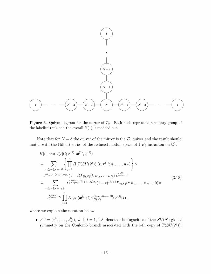
3.2 The Coulomb branch of the mirror of TN
The case of a sphere with three maximal punctures ρ = (1, · · · , 1) is known as the TNtheory [5]. We can compute the Coulomb branch Hilbert series of the mirror of the
TN theory reduced to three dimensions by gluing three T (SU(N)) tails together. The
quiver diagram of such a mirror theory is depicted in Figure 3.
– 15 –
N N − 1N − 1
N − 1
N − 2
N − 2N − 2 · · ·· · ·
...
11
1
Figure 3. Quiver diagram for the mirror of TN . Each node represents a unitary group of
the labelled rank and the overall U(1) is modded out.
Note that for N = 3 the quiver of the mirror is the E6 quiver and the result should
match with the Hilbert series of the reduced moduli space of 1 E6 instanton on C2.
H[mirror TN ](t;x(1),x(2),x(3))
=∑
n1≥···≥nN=0
{3∏j=1
H[T (SU(N))](t;x(j);n1, . . . , nN)
}×
t−δU(N)(n1,...,nN )(1− t)PU(N)(t;n1, . . . , nN) ε∑Ni=1 ni
=∑
n1≥···≥nN−1≥0
t12
∑N−1j=1 (N+1−2j)nj(1− t)3N+1PU(N)(t;n1, . . . , nN−1, 0)×
ε∑N−1i=1 ni
3∏j=1
K(1N )(x(j); t)Ψ
(n1,...,nN−1,0)
U(N) (x(j); t) ,
(3.18)
where we explain the notation below:
• x(i) = (x(i)1 , . . . , x
(i)N ), with i = 1, 2, 3, denotes the fugacities of the SU(N) global
symmetry on the Coulomb branch associated with the i-th copy of T (SU(N));
– 16 –

they satisfy
N∏k=1
x(i)k = 1 , with i = 1, 2, 3 . (3.19)
• The second line of the first equality is the gluing factor for the U(N) group:
1. δU(N) denotes the contribution from the U(N) background vector multiplet:
δU(N)(n1, . . . , nN) =∑
1≤i<j≤N
|ni − nj|
=N∑j=1
(N + 1− 2j)nj , n1 ≥ n2 ≥ · · · ≥ nN ≥ 0 .
(3.20)
2. The removal of the overall U(1) is done in two steps:
(a) Multiplying (1− t) to the function PU(N)(t;n1, . . . , nN).
(b) Restricting nN = 0.
• The prefactor K(1N )(x; t) is given by
K(1N )(x; t) = PE[χU(N)Adj (x)t
]. (3.21)
• The fugacity ε, with εN = 1, corresponds to a potential ZN discrete topological
symmetry for the U(N) gauge group modulo U(1). In the notations of section 3
of [1], the ZN valued fugacity is related to the ambiguity in taking the N -th root
when solving the constraint on the topological fugacities for z0:
z0 = εz0 , with z0 :=
(e∏
a=1
da∏k=1
zNk,ak,a
)1/N
, (3.22)
where z0 denotes the N -th principal root and ε runs over N -th roots of unity,
εN = 1 , (3.23)
and Nk,a and zk,a are the rank and the fugacity for the topological symmetry of
the k-th gauge group in the a-th leg. Often all or part of this ZN symmetry can
be absorbed in the center of the continuous topological symmetry associated to
zk,a. For this reason we will sometimes omit ε in the following.
– 17 –
Our result should agree with the Higgs branch Hilbert series of the TN theory. The
latter can be evaluated in the 4d version of the theory, since the Higgs branch does not
depend on the dimension. Let us compare (3.18) with the result in [4] for the Higgs
branch Hilbert series of TN which is computed by the 4d Hall-Littlewood index. In
that reference, the HL polynomial is defined with a normalization factor:4
ΨλU(N)(x1, . . . , xN ; t) = Nλ(t)Ψλ
U(N)(x1, . . . , xN ; t) . (3.24)
The normalization Nλ(t) is given by
N−2λ1,...λk
(t) =∞∏i=0
m(i)∏j=1
(1− tj
1− t
), (3.25)
where m(i) is the number of rows in the Young diagram λ = (λ1, . . . , λN) of length i.
It is related to PU(N) as follows:
(1− t)NPU(N)(t;n1, . . . , nN−1, 0) = Nn1,...,nN−1,0(t)2 . (3.26)
Using the identity
(1− t)2N+1t12
∑N−1j=1 (N+1−2j)nj =
(1− t)N+2∏N
i=2(1− ti)Ψ
(n1,...,nN−1,0)
U(N) (t12
(N−1), t12
(N−3), . . . , t−12
(N−1); t), (3.27)
we arrive at
H[mirror TN ](t;x(1),x(2),x(3))
= (1− t)N+2
{N∏i=2
(1− ti)
}K(1N )(x
(1); t)K(1N )(x(2); t)K(1N )(x
(3); t)×
∑n1≥n2≥···≥nN−1≥0
Ψ(n1,...,nN−1,0)
U(N) (x(1); t)Ψ(n1,...,nN−1,0)
U(N) (x(2); t)Ψ(n1,...,nN−1,0)
U(N) (x(3); t)
Ψ(n1,...,nN−1,0)
U(N) (t12
(N−1), t12
(N−3), . . . , t−12
(N−1); t),
(3.28)
where the normalized HL polynomial ΨnU(N)(x; t) is defined as in (3.24). Our result
agrees with formula (5.33) of [4].
3.3 The Coulomb branch of the mirror of a general 3d Sicilian theory
The computation of the Coulomb branch Hilbert series for the mirror of TN can be
easily generalized to a general 3d Sicilian theory. For the mirror of a theory that arises
4Our fugacity t is related to τ in [4] by τ = t1/2.
– 18 –
from a compactification of the AN−1 6d (2, 0) theory on a circle times a genus g Riemann
surface with punctures {ρ1,ρ2, . . . ,ρe}, the Coulomb branch Hilbert series is given by
H[mirror g, {ρ1,ρ2, . . . ,ρe}](t;x(1), . . . ,x(e))
=∑
n1≥···≥nN=0
{e∏j=1
H[Tρj(SU(N))](t;x(j);n1, . . . , nN)
}×
tδU(N), g(n1,...,nN )(1− t)PU(N)(t;n1, . . . , nN),
(3.29)
where the contribution of the g U(N) adjoint hypermultiplets and vector multiplet to
the dimension of monopole operators is
δU(N), g(n) = (g − 1)δU(N)(n) = (g − 1)∑
1≤i<j≤N
|ni − nj|
= (g − 1)N∑j=1
(N + 1− 2j)nj , n1 ≥ · · · ≥ nN ≥ 0 ,
with δU(N)(n1, . . . , nN) given by (3.30). We therefore obtain
H[mirror g, {ρ1,ρ2, . . . ,ρe}](t;x(1), . . . ,x(e))
=∑
n1≥···≥nN−1≥0
t(e2
+g−1)∑N−1j=1 (N+1−2j)nj(1− t)eN+1PU(N)(t;n1, . . . , nN−1, 0)×
e∏j=1
Kρj(x(j); t)Ψ
(n1,...,nN−1,0)
U(N) (x(j)t12wρj ; t) ,
(3.30)
3.3.1 The case of genus zero
In a special case of g = 0, we use (3.26) and (3.27) to obtain
H[mirror {ρ1,ρ2, . . . ,ρe}](t;x(1), . . . ,x(e))
= (1− t)e+(N−1)
{N∏i=2
(1− ti)
}e−2
×
∑n1≥n2≥···≥nN−1≥0
∏ej=1Kρj(x
(j); t)Ψ(n1,...,nN−1,0)
U(N) (x(j)t12wρj ; t)
[Ψ(n1,...,nN−1,0)
U(N) (t12
(N−1), t12
(N−3), . . . , t−12
(N−1); t)]e−2,
(3.31)
where ΨU(N) denotes the normalized Hall-Littlewood polynomial defined in (3.24). This
result agrees with the Higgs branch Hilbert series of the Gaiotto theory, computed as
a Hall-Littlewood index for g = 0 in (2.13) of [9].
– 19 –

3k
2k
k
2k kk 2k 1
(a)
4k
3k
2k
2k k2k 1
k
3k
(b)
6k
4k
2k
3k 5k
(c)
4k 2k k 13k
Figure 4. The moduli spaces of k E6, E7 and E8 instantons on C2 can be realized using
the Coulomb branch of quiver diagrams (a), (b) and (c) respectively. Each node represents a
unitary group of the labelled rank and the overall U(1) is modded out in each diagram.
As discussed in [9], the formula (3.31) can be used to write the Hilbert series for
the moduli spaces of E6, E7 and E8 instantons on C2, which can be realized as the
Higgs branch of the 6d (2, 0) theory compactified on a Riemann sphere with punctures
{ρ1,ρ2,ρ3}
ρ1 ρ2 ρ3
E6 (k, k, k) (k, k, k) (k, k, k − 1, 1)
E7 (k, k, k, k) (2k, 2k) (k, k, k, k − 1, 1)
E8 (3k, 3k) (2k, 2k, 2k) (k, k, k, k, k, k − 1, 1)
(3.32)
corresponding to the mirror quiver given in Figure 4.
3.3.2 Mirror of the SU(3) Sicilian theory with g = 1 and a maximal puncture
Recall that for genus g > 0 the HL index differs from the Higgs branch Hilbert series
of the Sicilian theory [4]. The latter is given by our formula (3.30), assuming mirror
symmetry.
Let us provide an explicit example for the case of N = 3, g = 1 and one maximal
puncture ρ = (1, 1, 1) below. The quiver diagram of the mirror theory of our interest
is depicted in Figure 5. This example is particularly interesting because the global
– 20 –

symmetry on the Coulomb branch enhances to G2 [9]. We will show this by computing
the Hilbert series and expanding it in G2 characters.
1 2 3
Figure 5. Quiver for the mirror of the A2 theory on a circle times a torus with one maximal
puncture. The overall U(1) is factored out.
The Coulomb branch Hilbert series can be computed using (3.30), where the fu-
gacities x1, x2, x3 are related to the fugacities for the topological charges of U(1), U(2)
and U(3) gauge groups and are subject to the constraint (2.13). In order to make G2
characters manifest in the Hilbert series, we use the fugacity map5
x1 = y1, x2 = y1y−12 , x3 = y−2
1 y2 , (3.33)
where x1, x2 are the fugacities in formula (3.30) and y1, y2 are the G2 fugacities.
We then obtain
H[mirror g = 1, (1, 1, 1)](t; y1, y1y−12 , y2y
−21 ) = f(0, 0, 0) + f(3, 1, 5) , (3.34)
where
f(a, b, c) =∞∑
n1=0
∞∑n2=0
∞∑n3=0
∞∑n4=0
[2n2 + 3n3 + a, n1 + 2n4 + b]tn1+2n2+3n3+4n4+c , (3.35)
and [a, b] denotes the character of the G2 representation with highest weight [a, b],
written in terms of y1, y2. The character expansion (3.34) shows not only that the
adjoint representation arises at ∆ = 1 (for the scalar partners of conserved currents),
but also that the whole chiral spectrum transforms in G2 representations as expected.
The unrefined Hilbert series is given by
H[mirror g = 1, (1, 1, 1)](t; 1, 1, 1) =1 + 4t+ 9t2 + 9t3 + 4t4 + t5
(1− t)10, (3.36)
with a palindromic numerator and a pole at t = 1 of order 10, equal to the complex
dimension of the Coulomb branch of the moduli space.
5Here we use the characters of G2 as in LiE online service at the following link:
http://young.sp2mi.univ-poitiers.fr/cgi-bin/form-prep/marc/LiE_form.act?action=
character&type=G&rank=2&highest_rank=8.
– 21 –
The generating function of highest weights [24]. The highest weight vectors
that appear in formula (3.34) can be collected in the following generating function:
PE[µ2t+ µ21t
2 + µ31t
3 + µ22t
4 + µ31µ2t
5 − µ61µ
22t
10]
=1− t10µ6
1µ22
(1− t2µ21) (1− t3µ3
1) (1− tµ2) (1− t5µ31µ2) (1− t4µ2
2),
(3.37)
where µ1 and µ2 are the fugacities associated with the highest weights n1 and n2 of
representations of G2. Upon computing the power series in t of (3.37), the powers
µn11 µ
n22 can be traded for the Dynkin label [n1, n2] to obtain the character expansion as
stated in (3.34). Let us demonstrate this for the first few terms in the power series:
1 + µ2t+(µ2
1 + µ22
)t2 +
(µ3
1 + µ21µ2 + µ3
2
)t3 + . . . . (3.38)
Trading the powers of µ1 and µ2 for the Dynkin label, we obtain
1 + [0, 1]t+ ([2, 0] + [0, 2])t2 + ([3, 0] + [2, 1] + [0, 3])t3 + . . . . (3.39)
4 Mirrors of 3d Sicilian theories of D-type
In this section we consider three dimensional theories arising from the 6d (2, 0) theory
of DN type compactified on a circle times a Riemann surface with punctures. Each
puncture is classified by a D-partition of SO(2N). The Coulomb branch Hilbert series
of the mirror theory can be computed by gluing copies of the Tρ(SO(2N)) theories
[6] according to the general discussion in section 3. The quivers for the Tρ(SO(2N))
theories, which can be realised from brane and orientifold configurations as in [25],
are reviewed in section 4.2 of [3]. We remark that we gauge the centerless group
SO(2N)/Z2 rather than SO(2N). Consequently, the magnetic fluxes of the gluing
gauge group belong to the weight lattice of the dual group Spin(2N) modulo the Weyl
group.
Given a 3d Sicilian theory with genus g and e D-type punctures {ρ1,ρ2, . . . ,ρe},the Coulomb branch Hilbert series of its mirror theory is6
H[mirror g, {ρ1,ρ2, . . . ,ρe}](t;x(1), . . . ,x(e))
=∑
n1≥···≥nN−1≥|nN |
{e∏j=1
H[Tρj(SO(2N))](t;x(j);n1, . . . , nN)
}×
tδSO(2N), g(n1,...,nN )PSO(2N)(t;n1, . . . , nN),
(4.1)
6It is straightforward to include in (4.1) a fugacity for the center of Spin(2N), but we prefer not
to clutter formulae with those factors, which can often be reabsorbed.
– 22 –
where H[Tρ(SO(2N))] is given by (2.21), the Casimir factor PSO(2N) is computed as in
(2.2) (see (A.10) of [1] for an explicit expression), and δSO(2N), g(n) is the contribution
of the g SO(2N) adjoint hypermultiplets and vector multiplet to the dimension of
monopole operators is
δSO(2N), g(n) = (g − 1)δSO(2N)(n) = (g − 1)N−1∑j=1
(2N − 2j)nj , (4.2)
with the second equality following from (2.24). Note that because the dual of the gluing
group is Spin(2N), n1, . . . , nN are all integers or all half-odd integers.
For g = 0 our formula (4.1) for the Coulomb branch Hilbert series of mirrors of
D-type Sicilian theories proposed in [6] agrees with the Higgs branch Hilbert series of
the Sicilian theory, computed as the Hall-Littlewood limit of the superconformal index
of the 4d Sicilian theory in formula (4.10) of [10].7 For higher genus the HL index does
not compute the Hilbert series of the Higgs branch. Formula (4.1) provides a prediction
for the latter, assuming mirror symmetry.
In the rest of the section we provide examples of Sicilian theories with D3 and
D4 symmetry and we compare with the results in [10, 26]. We start this section by
considering the case of D3. Due to the isomorphism of its Lie algebra with that of A3,
each D3 puncture can be identified with an A3 puncture. We compute the Coulomb
branch Hilbert series of mirror theories of 3d Sicilian theories with D3 punctures using
the Hall-Littlewood formula and compare the result with those with A3 punctures.
We then consider D4 theories with a set of punctures for which the Higgs branch is
explicitly known and we compare our result for the Coulomb branch Hilbert series of
the mirror with the Higgs branch Hilbert series. The case of twisted D punctures is
discussed in the Appendix. All these examples demonstrate the validity of our formula
(4.1).
4.1 D3 punctures
There are four possible D-partitions of SO(6). These partitions and the identification
with A3 partitions are given on Page 17 of [26]. We list them as follows in Table 1.
7The orthonormal Hall-Littlewood polynomials used in [10] can be expressed in terms of the
Hall-Littlewood polynomials used here as PnM G(a|0, t) = (1 − t)rk(G)/2PG∨(t;n)1/2Ψn
G(a(t,x); t).
The pre-factors are related by KG = (1 − t)rk(G)/2KG. Finally, for G = SO(2N) one finds
A(0, t)/PnM SO(2N)(1, t, t
2, . . . , tN−1|0, t) = t12 δSO(2N)(n)PSO(2N)(t;n)−1/2.
– 23 –
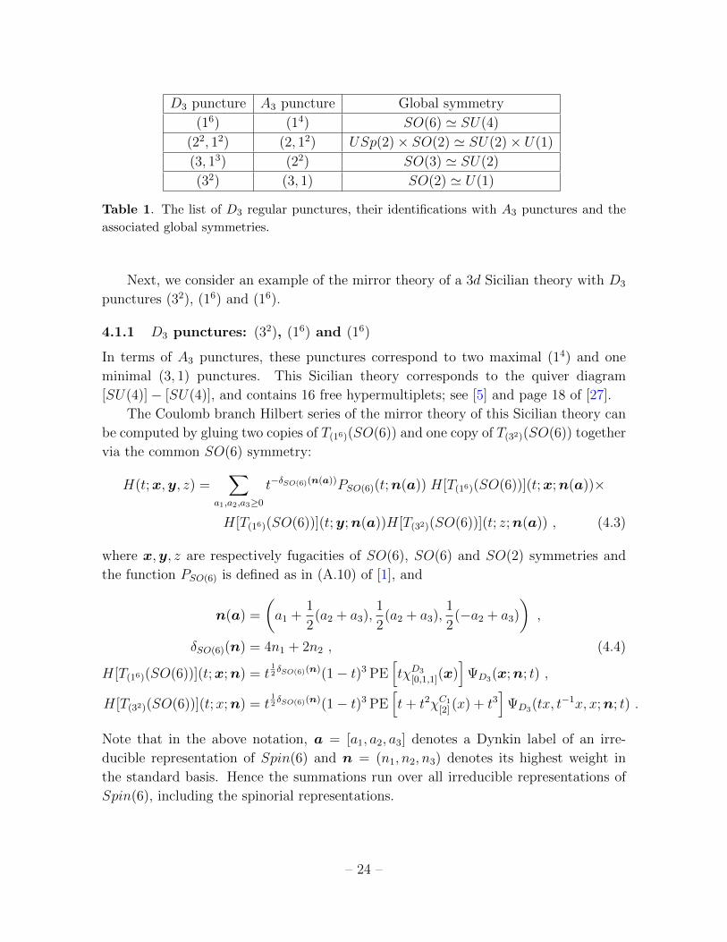
D3 puncture A3 puncture Global symmetry
(16) (14) SO(6) ' SU(4)
(22, 12) (2, 12) USp(2)× SO(2) ' SU(2)× U(1)
(3, 13) (22) SO(3) ' SU(2)
(32) (3, 1) SO(2) ' U(1)
Table 1. The list of D3 regular punctures, their identifications with A3 punctures and the
associated global symmetries.
Next, we consider an example of the mirror theory of a 3d Sicilian theory with D3
punctures (32), (16) and (16).
4.1.1 D3 punctures: (32), (16) and (16)
In terms of A3 punctures, these punctures correspond to two maximal (14) and one
minimal (3, 1) punctures. This Sicilian theory corresponds to the quiver diagram
[SU(4)]− [SU(4)], and contains 16 free hypermultiplets; see [5] and page 18 of [27].
The Coulomb branch Hilbert series of the mirror theory of this Sicilian theory can
be computed by gluing two copies of T(16)(SO(6)) and one copy of T(32)(SO(6)) together
via the common SO(6) symmetry:
H(t;x,y, z) =∑
a1,a2,a3≥0
t−δSO(6)(n(a))PSO(6)(t;n(a)) H[T(16)(SO(6))](t;x;n(a))×
H[T(16)(SO(6))](t;y;n(a))H[T(32)(SO(6))](t; z;n(a)) , (4.3)
where x,y, z are respectively fugacities of SO(6), SO(6) and SO(2) symmetries and
the function PSO(6) is defined as in (A.10) of [1], and
n(a) =
(a1 +
1
2(a2 + a3),
1
2(a2 + a3),
1
2(−a2 + a3)
),
δSO(6)(n) = 4n1 + 2n2 , (4.4)
H[T(16)(SO(6))](t;x;n) = t12δSO(6)(n)(1− t)3 PE
[tχD3
[0,1,1](x)]
ΨD3(x;n; t) ,
H[T(32)(SO(6))](t;x;n) = t12δSO(6)(n)(1− t)3 PE
[t+ t2χC1
[2] (x) + t3]
ΨD3(tx, t−1x, x;n; t) .
Note that in the above notation, a = [a1, a2, a3] denotes a Dynkin label of an irre-
ducible representation of Spin(6) and n = (n1, n2, n3) denotes its highest weight in
the standard basis. Hence the summations run over all irreducible representations of
Spin(6), including the spinorial representations.
– 24 –

It can be checked that the first few terms in the power series of (4.3) are equal to
those of the Hilbert series of 16 free hypermultiplets in the spinor representations of
SO(6), as expected from mirror symmetry:
H(t;x,y, z) = PE[{z1/2χD3
[0,1,0](x)χD3
[0,1,0](y) + z−1/2χD3
[0,0,1](x)χD3
[0,0,1](y)}t]
=∞∑
n1,n2,n3=0
χD3
[n2,n1,n3](x)χD3
[n2,n1,n3](y)(z1/2t)n1+2n2+3n3×
∞∑m1,m2,m3=0
χD3
[m2,m3,m1](x)χD3
[m2,m3,m1](y)(z−1/2t)m1+2m2+3m3 . (4.5)
4.2 D4 punctures
In this section, we provide three examples on Sicilian theories with the following D4
punctures.
1. (5, 3), (22, 14) and (18) ,
2. (32, 12), (22, 14) and (22, 14) ,
3. (5, 3), (5, 3), (24) and (3, 15) .
In the following subsections, we compute the Coulomb branch Hilbert series of the
mirror theories of these Sicilian theories and compare the results to those presented in
[26].
For reference, we tabulate the quiver diagrams for Tρ(SO(8), with ρ being parti-
tions listed above, in Table 2.
Partition ρ Quiver diagram for Tρ(SO(8))
(5, 3) [SO(8)]− (USp(2))
(32, 12) [SO(8)]− (USp(4))− (SO(2))
(24) [SO(8)]− (USp(6))− (SO(4))− (USp(2))
(3, 15) [SO(8)]− (USp(4))− (SO(4))− (USp(2))− (SO(2))
(22, 14) [SO(8)]− (USp(6))− (SO(4))− (USp(2))− (SO(2))
(18) [SO(8)]− (USp(6))− (SO(6))− (USp(4))− (SO(4))− (USp(2))− (SO(2))
Table 2. Quiver diagrams for Tρ(SO(8)) for certain D4 partitions ρ.
– 25 –
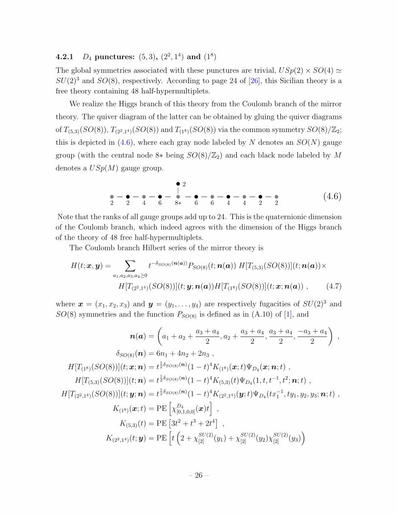
4.2.1 D4 punctures: (5, 3), (22, 14) and (18)
The global symmetries associated with these punctures are trivial, USp(2)× SO(4) 'SU(2)3 and SO(8), respectively. According to page 24 of [26], this Sicilian theory is a
free theory containing 48 half-hypermultiplets.
We realize the Higgs branch of this theory from the Coulomb branch of the mirror
theory. The quiver diagram of the latter can be obtained by gluing the quiver diagrams
of T(5,3)(SO(8)), T(22,14)(SO(8)) and T(18)(SO(8)) via the common symmetry SO(8)/Z2;
this is depicted in (4.6), where each gray node labeled by N denotes an SO(N) gauge
group (with the central node 8∗ being SO(8)/Z2) and each black node labeled by M
denotes a USp(M) gauge group.
•2− •
2− •
4− •
6−• 2|•8∗− •
6− •
6− •
4− •
4− •
2− •
2(4.6)
Note that the ranks of all gauge groups add up to 24. This is the quaternionic dimension
of the Coulomb branch, which indeed agrees with the dimension of the Higgs branch
of the theory of 48 free half-hypermultiplets.
The Coulomb branch Hilbert series of the mirror theory is
H(t;x,y) =∑
a1,a2,a3,a4≥0
t−δSO(8)(n(a))PSO(8)(t;n(a)) H[T(5,3)(SO(8))](t;n(a))×
H[T(22,14)(SO(8))](t;y;n(a))H[T(18)(SO(8))](t;x;n(a)) , (4.7)
where x = (x1, x2, x3) and y = (y1, . . . , y4) are respectively fugacities of SU(2)3 and
SO(8) symmetries and the function PSO(8) is defined as in (A.10) of [1], and
n(a) =
(a1 + a2 +
a3 + a4
2, a2 +
a3 + a4
2,a3 + a4
2,−a3 + a4
2
),
δSO(8)(n) = 6n1 + 4n2 + 2n3 ,
H[T(18)(SO(8))](t;x;n) = t12δSO(8)(n)(1− t)4K(18)(x; t)ΨD4(x;n; t) ,
H[T(5,3)(SO(8))](t;n) = t12δSO(8)(n)(1− t)4K(5,3)(t)ΨD4(1, t, t−1, t2;n; t) ,
H[T(22,14)(SO(8))](t;y;n) = t12δSO(8)(n)(1− t)4K(22,14)(y; t)ΨD4(tx−1
1 , ty1, y2, y3;n; t) ,
K(18)(x; t) = PE[χD4
[0,1,0,0](x)t],
K(5,3)(t) = PE[3t2 + t3 + 2t4
],
K(22,14)(t;y) = PE[t(
2 + χSU(2)[2] (y1) + χ
SU(2)[2] (y2)χ
SU(2)[2] (y3)
)
– 26 –

+ t3/2χSU(2)[2] (y1){χSU(2)
[2] (y2) + χSU(2)[2] (y3)}+ t2
]. (4.8)
It can be checked that the first few terms in the power series of (4.7) agrees with
H(t;x,y) = PE[{χD4
[1,0,0,0](x)χSU(2)[1] (y1) + χD4
[0,0,1,0](x)χSU(2)[1] (y2)
+ χD4
[0,0,0,1](x)χSU(2)[1] (y3)
}t],
(4.9)
namely the Hilbert series of 48 free half-hypermultiplets, as expected from mirror sym-
metry.
4.2.2 D4 punctures: (32, 12), (22, 14) and (22, 14)
The quiver diagram of the mirror of this Sicilian theory can be obtained by gluing the
quiver diagrams of T(32,12)(SO(8)), T(22,14)(SO(8)) and T(22,14)(SO(8)) via the common
symmetry SO(8)/Z2; this is depicted in (4.10), where each gray node labeled by N
denotes an SO(N) gauge group (with the central node 8∗ being SO(8)/Z2) and each
black node labeled by M denotes a USp(M) gauge group.
•2− •
2− •
4− •
6−
•2|• 4|•8∗− •
6− •
4− •
2− •
2(4.10)
The quaternionic dimension of the Coulomb branch of this theory, equal to the sum
of the ranks of all gauge groups, is 21.
The global symmetries associated with these punctures are respectively SO(2)2,
SU(2)3 and SU(2)3. According to page 28 of [26], this Sicilian theory can be identified
with the T4 theory and the global symmetry enhances to SU(4)3. Indeed, the Higgs
branch of the T4 theory is 21 quaternionic dimensional; this is in agreement with the
dimension of the Coulomb branch of the mirror theory.
The Coulomb branch Hilbert series of theory depicted in (4.10) is
H(t;x,y, z) =∑
a1,a2,a3,a4≥0
t−δSO(8)(n(a))PSO(8)(t;n(a)) H[T(32,12)(SO(8))](t; z;n(a))×
H[T(22,14)(SO(8))](t;y;n(a))H[T(22,14)(SO(8))](t;x;n(a)) , (4.11)
where x = (x1, x2, x3) and y = (y1, y2, y3) are fugacities for SU(2)3, z = (z1, z2) are
fugacities for SO(2)2, and
H[T(32,12)(SO(8))](t; z;n) = t12δSO(8)(n)(1− t)4K(32,12)(z; t)ΨD4(z1t, z1t
−1, z1, z2;n; t) ,
– 27 –
K(32,12)(z; t) = PE
[2t+
(z2
1 + 1 + z−21 +
∑ε1,ε2=±1
zε11 zε22
)t2 + t3
].
(4.12)
Computing the power series in t of the above expression (4.11), we find that at
order t, the 45 gauge invariants transform as follows:
(z1 + z−11 )[1]x1 [1]y1 + [2]x1 + [2]y1 + 1
+ (z1/21 z
1/22 + z
−1/21 z
−1/22 )[1]x2 [1]y2 + [2]x2 + [2]y2 + 1
+ (z1/21 z
−1/22 + z
−1/21 z
1/22 )[1]x3 [1]y3 + [2]x3 + [2]y3 + 1 ,
(4.13)
where [· · · ]a denotes the character of representation [· · · ] written in terms of a. Note
that each line gives the decomposition of the adjoint representation of SU(4) in terms
of representations of SO(2) × SU(2)2. Hence these 45 generators indeed decompose
into three copies of 15, each transforming in the adjoint representation of an SU(4) in
SU(4)3.
A similar analysis can be performed at higher orders of t. Moreover, the unrefined
Hilbert series, i.e. all xi, yi, zi are set to 1, can be computed from (4.11):
H(t; 1,1,1) = 1 + 45t+ 128t3/2 + 1249t2 + 5504t5/2 + . . . ; (4.14)
the result is in agreement with [4].
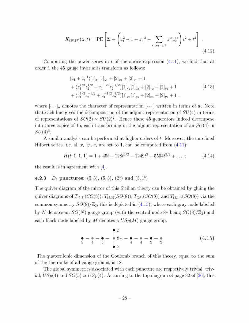
4.2.3 D4 punctures: (5, 3), (5, 3), (24) and (3, 15)
The quiver diagram of the mirror of this Sicilian theory can be obtained by gluing the
quiver diagrams of T(5,3)(SO(8)), T(5,3)(SO(8)), T(24)(SO(8)) and T(3,15)(SO(8)) via the
common symmetry SO(8)/Z2; this is depicted in (4.15), where each gray node labeled
by N denotes an SO(N) gauge group (with the central node 8∗ being SO(8)/Z2) and
each black node labeled by M denotes a USp(M) gauge group.
•2− •
4− •
6−• 2|•|• 2
8∗ − •4− •
4− •
2− •
2(4.15)
The quaternionic dimension of the Coulomb branch of this theory, equal to the sum
of the the ranks of all gauge groups, is 18.
The global symmetries associated with each puncture are respectively trivial, triv-
ial, USp(4) and SO(5) ' USp(4). According to the top diagram of page 32 of [26], this
– 28 –

Sicilian theory can be identified with the G2 gauge theory with 4 fundamental hyper-
multiplets and 4 free hypermultiplets, which has USp(8) flavor symmetry. Indeed, the
quaternionic dimension of the Higgs branch of this theory is equal to 12(7×4) + 4 = 18;
this is in agreement with the dimension of the Coulomb branch of the mirror theory.
The Higgs branch Hilbert series of G2 gauge theory with 4 flavors of funda-
mental hypers, plus 4 free hypers
In the following, we write
τ = t1/2 . (4.16)
The F -flat Hilbert series is given by
F [(τ ; z;x) = PE[τχ
USp(8)[1,0,0,0](x)
]× PE
[τχ
USp(8)[1,0,0,0](x)χG2
[1,0](z)− τ 2χG2
[0,1](z)]. (4.17)
The Higgs branch Hilbert series can be obtained by integrating over the G2 gauge group
as follows:
g(τ,x) =
∫dµG2(z) F [(τ ; z;x) , (4.18)
where the Haar measure of G2 is given by∫dµG2(z) =
1
(2πi)2
∮|z1|=1
dz1
z1
∮|z2|=1
dz2
z2
(1− z1)(1− z21z−12 )(1− z3
1z−12 )
(1− z2)(1− z2z−11 )(1− z2
2z−31 ) .
(4.19)
The first few terms in the power series of the Higgs branch Hilbert series g(τ,x) are
g(τ,x) = PE[τχC4
[1,0,0,0](x)]×{
1 + χC4
[2,0,0,0](x)τ 2 +(χC4
[1,0,0,0](x) + χC4
[0,0,1,0](x))τ 3
+(χC4
[4,0,0,0](x) + χC4
[0,1,0,0](x) + χC4
[0,2,0,0](x) + χC4
[0,0,0,1](x) + 1)τ 4 + . . .
}.
(4.20)
Below we reproduce this Hilbert series from the Coulomb branch of the mirror theory
of this Sicilian theory.
The Coulomb branch Hilbert series of the mirror theory
The Coulomb branch Hilbert series is given by
H(t;x,y) =∑
a1,a2,a3,a4≥0
t−δSO(8)(n(a))PSO(8)(t;n(a)) H[T(5,3)(SO(8))](t;n(a))×
H[T(5,3)(SO(8))](t;n(a))H[T(24)(SO(8))](t;y;n(a))×H[T(3,15)(SO(8))](t;x;n(a)) ,
(4.21)
– 29 –
where x = (x1, x2) and y = (y1, y2) are fugacities for SO(5) and USp(4) respectively,
and
H[T(3,15)(SO(8))](t;x;n) = t12δSO(8)(n)(1− t)4K(3,15)(x; t)ΨD4(1, t, x1, x2;n; t) ,
K(3,15)(x; t) = PE[tχB2
[0,2](x) + t2(1 + χB2
[1,0](x)].
(4.22)
We have checked that the first few terms in the power series of this Hilbert series agree
with (4.20). In particular, the unrefined Hilbert series is
H[T(3,15)(SO(8))](t,x = 1,y = 1) = 1 + 8t1/2 + 72t+ 464t3/2 + 2782t2 + . . .
=1
(1− t1/2)8(1 + 36t+ 56t3/2 + 708t2 + . . .) .
(4.23)
5 Coulomb branch Hilbert series of 3d theories with tri-vertices
In this section we consider the Coulomb branch of theories on two M5-branes compacti-
fied on a Riemann surface with punctures times a circle of vanishing size. The latter are
referred to as 3d SU(2) Sicilian theories [6, 23], or 3d theories with tri-vertices [11]. We
emphasize that in this section we aim to compute the Coulomb branch Hilbert series
of tri-vertex theories, in contrast to section 3.1.1 in which we considered the Coulomb
branch of their mirrors.
We follow the notation adopted in [11]. The Lagrangian of a tri-vertex theory is
specified by a graph made of tri-valent vertices connected by lines. Each line denotes
an SU(2) group; an internal line (of finite length) denotes a gauge group, whereas
an external line (of infinite length) denotes a flavor group. Each vertex denotes 8
half-hypermultiplets in the tri-fundamental representation of the corresponding SU(2)3
group. Such graphs are classified topologically by the genus g and the number e of
external legs. It was found in [11] that the Higgs branch of such theories depends only
on g and e and not on the details of how the vertices are connected to each other.
In this section we focus only on the cases with g = 0, i.e. tree diagrams, since
for higher genus the theory is bad. For g = 0, the Coulomb branch Hilbert series
can be evaluated explicitly and it depends only on the number of external legs e and
not on the details of the graph. In section 5.3 we present certain generating functions
and recursive formulae that serve as powerful tools for computing Hilbert series of
these class of theories using gluing techniques. The fact that such generating functions
depend solely on the number of external legs e is proven in section 5.3.2.
It would be interesting to understand how to compute the Coulomb branch Hilbert
series of theories with higher genus by determining whether they flow to a good theory
in the IR.
– 30 –
5.1 The case of g = 0
We consider the Coulomb branch of 3d N = 4 gauge theories based on tri-vertex
tree (g = 0) diagrams, with SU(2) gauge groups associated to internal edges and
tri-fundamental half-hypermultiplets associated to nodes.
We will see in a few examples that, as for the Higgs branch [11], the Coulomb
branch only depends on the number of external edges; see an example for g = 0 and
e = 6 in section 5.1.2 below. We give a general proof of this fact in subsection 5.3.2.
5.1.1 General formula for g = 0 and any e
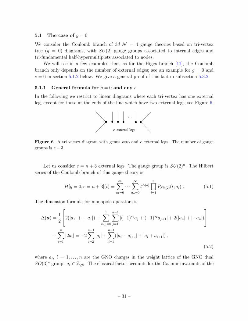
In the following we restrict to linear diagrams where each tri-vertex has one external
leg, except for those at the ends of the line which have two external legs; see Figure 6.
...
e external legs
Figure 6. A tri-vertex diagram with genus zero and e external legs. The number of gauge
groups is e− 3.
Let us consider e = n + 3 external legs. The gauge group is SU(2)n. The Hilbert
series of the Coulomb branch of this gauge theory is
H[g = 0, e = n+ 3](t) =∞∑a1=0
· · ·∞∑
an=0
t∆(a)
n∏i=1
PSU(2)(t; ai) . (5.1)
The dimension formula for monopole operators is
∆(a) =1
2
2(|a1|+ |−a1|) +1∑
s1,2=0
n−1∑j=1
|(−1)s1aj + (−1)s2aj+1|+ 2(|an|+ |−an|)
−
n∑i=1
|2ai| = −2n−1∑i=2
|ai|+n−1∑i=1
(|ai − ai+1|+ |ai + ai+1|) ,
(5.2)
where ai, i = 1, . . . , n are the GNO charges in the weight lattice of the GNO dual
SO(3)n group: ai ∈ Z≥0. The classical factor accounts for the Casimir invariants of the
– 31 –

residual gauge group which is not broken by the monopole flux. For an SU(2) gauge
group, the classical factor is
PSU(2)(t; a) =
{1
1−t2 , a = 01
1−t , a > 0. (5.3)
The result for the Hilbert series (5.1) appears to be
H[g = 0, e = n+ 3](t) =
∑nj=0
(nj
) [(nj
)t2j −
(nj+1
)t2j+1
](1− t)2n(1 + t)n
=1
(1− t)2n(1 + t)n
[− nt 2F1(1− n,−n; 2; t2) + 2F1(−n,−n; 2; t2)
].
(5.4)
5.1.2 Special case of g = 0 and e = 6
As an example of the fact that the Coulomb branch only depends on the number of
external edges we consider the case e = 6. There are two diagrams corresponding to
g = 0 and e = 6, depicted in Figure 7.
(a) (b)
Figure 7. Two tri-vertex diagrams with genus zero and 6 external legs.
Diagram (a). The Coulomb branch Hilbert series of diagram (a) is given by (5.4):
H(a)(t) =1− 3t+ 9t2 − 9t3 + 9t4 − 3t5 + t6
(1− t)6(1 + t)3(5.5)
Diagram (b). For diagram (b), we have
∆(b)(a) =1
2
1
2
1∑s1,2,3=0
∣∣∣∣∣3∑i=1
(−1)siai
∣∣∣∣∣+ 23∑i=1
(|ai|+ |−ai|)
− 3∑i=1
|2ai| , (5.6)
Observe that this is not equal to ∆(a)(a) which is given in (5.2). However, the Hilbert
series of the Coulomb branch is given by
H(b)(t) =∞∑
a1,a2,a3=0
t∆(b)(a)
3∏i=1
PSU(2)(t; ai)
=1− 3t+ 9t2 − 9t3 + 9t4 − 3t5 + t6
(1− t)6(1 + t)3= H(a)(t) ,
(5.7)
– 32 –
which is indeed equal to that of diagram (a).
5.2 Turning on background fluxes
So far we have computed the Coulomb Hilbert series without considering the back-
ground monopole charges coming from the global symmetries of the theory. In this
section, we turn on such background charges for the flavor symmetries present in the
theory and the corresponding Hilbert series will, of course, depend on such charges.
This will turn out to be extremely useful in subsequent computations.
Let us first consider the T2 theory (g = 0, e = 3). The Coulomb branch Hilbert
series with background fluxes turned on is simply
H[T2](t; a1, a2, a3) = t∆g=0,e=3(a1,a2,a3) , (5.8)
where a1, a2, a3 ≥ 0 are the background fluxes and
∆g=0,e=3(a1, a2, a3) =1
2
1
2
1∑s1,2,3=0
|(−1)s1a1 + (−1)s2a2 + (−1)s3a3|
. (5.9)
The Coulomb branch Hilbert series with background fluxes turned on can be han-
dled more easily if we introduce extra fugacities to keep track of such background
charges. In this way, we end up computing the generating function of the Coulomb
branch Hilbert series. This is the topic of the next section.
5.3 Generating functions of Coulomb branch Hilbert series
For a theory with genus zero and e external legs, we can construct a generating function
Ge(z1, . . . , ze) =∞∑a1=0
· · ·∞∑ae=0
H[e](t; a1, . . . , ae)e∏i=1
zaii , (5.10)
where a1, . . . , ae are the background fluxes for the SU(2)e global symmetry group asso-
ciated to the external legs and H[e](t; a1, . . . , ae) is the usual Hilbert series with these
background fluxes turned on. Note that we omit the t dependence in Ge(z1, . . . , ze) for
the sake of brevity. To turn off the background fluxes, we simply set all zi to zero:
H[e](t; 0, . . . , 0) = Ge(0, 0, . . . , 0) . (5.11)
We go over the computations of generating functions in the examples below.
– 33 –

The T2 theory. From (5.8), we have
Ge=3(z1, z2, z3) =∞∑a1=0
∞∑a2=0
∞∑a3=0
t∆e=3(a)za11 z
a22 z
a33 , (5.12)
Evaluating the summations, we obtain
Ge=3(z) =1∏3
i=1(1− t2zi)∏
1≤j<k≤3(1− t2zjzk)×[1 + z1z2z3t
3
+ (−z1z2 − z1z3 − z2z3 − 3z1z2z3) t4 +(−z2
1z2z3 − z1z22z3 − z1z2z
23
)t5
+ 2(z1z2z3 + z2
1z2z3 + z1z22z3 + z1z2z
23
)t6 +
(z2
1z22z3 + z2
1z2z23 + z1z
22z
23
)t7
+(−z2
1z22z3 − z2
1z2z23 − z1z
22z
23
)t8 − z2
1z22z
23t
9]. (5.13)
Observe that Ge=3(z) is invariant under the permutations of z1, z2, z3. Upon setting
z1 = z2 = z3 = 0, we recover the (trivial) Hilbert series of the Coulomb branch as
expected:
Ge=3(0, 0, 0) = 1 . (5.14)
5.3.1 Gluing generating functions and recursive formula
If we glue a tree diagram with e1 external legs with another tree diagram with e2
external legs via an external leg, the resulting diagram is a tree diagram of e1 + e2 − 2
external legs. In terms of the Coulomb branch Hilbert series, this gluing operation can
be formulated as
H[e1 + e2 − 2](a)
=∞∑a=0
H[e1](a1, . . . , ae1−1, a)PSU(2)(t; a)t−2aH[e2](a, ae1 , . . . , ae1+e2−2) ,(5.15)
where in this formula we glue the e1-th external leg of the first diagram with the first
leg of the second diagram. In terms of the generating functions, we have
Ge1+e2−2(a) =
∮|u|=1
du
2πiu
∮|w|=1
du
2πiw
∞∑a=0
Ge1(z1, . . . , ze1−1, u)×
u−aPSU(2)(t; a)t−2aw−aGe2(w, ze1 , . . . , ze1+e2−2) ,
(5.16)
The recursive formula
The diagrams with g = 0 and e + 1 external legs can be constructed recursively by
gluing the diagram (g = 0, e = 3) with another diagram with e external legs. We can
thus obtain the recursive formula for the generating functions as follows.
– 34 –
From (5.16) we obtain
Ge+1(z) =
∮|u|=1
du
2πiu
∮|w|=1
dw
2πiw
∞∑a=0
Ge=3(z1, z2, u)×
u−aPSU(2)(t; a)t−2aw−aGe(w, z3, . . . , ze+1) .
(5.17)
We write the infinite sum as follows:
∞∑a=0
u−aPSU(2)(t; a)t−2aw−a = − t
1− t2+
t2uw
(1− t)(t2uw − 1). (5.18)
Thus we have
Ge+1(z) = − t
1− t2
∮|u|=1
du
2πiu
∮|w|=1
dw
2πiwGe=3(z1, z2, u)Ge(w, z3, . . . , ze+1)
+t2
1− t
∮|u|=1
du
2πi
∮|w|=1
dw
2πi
Ge=3(z1, z2, u)Ge(w, z3, . . . , ze+1)
t2uw − 1
= − t
1− t2Ge=3(z1, z2, 0)Ge(0, z3, . . . , ze+1)+
+1
1− t
∮|w|=1
dw
2πi
Ge=3(z1, z2, w−1t−2)Ge(w, z3, . . . , ze+1)
w.
(5.19)
In the integral of the last line, we see from (5.13) that the poles of Ge=3(z1, z2, w−1t−2)
are at w = 1, w = z1 and w = z2. Using the residue theorem, we obtain
Ge+1(z) = − t
1− t2Ge=3(z1, z2, 0)Ge(0, z3, . . . , ze+1)+
+1
(1− t)Res[Ge=3(z1, z2, w
−1t−2);w = 1]Ge(1, z3, . . . , ze+1)
+1
(1− t)z1
Res[Ge=3(z1, z2, w
−1t−2);w = z1
]Ge(z1, z3, . . . , ze+1)
+1
(1− t)z2
Res[Ge=3(z1, z2, w
−1t−2);w = z2
]Ge(z2, z3, . . . , ze+1) .
(5.20)
Using (5.13), we find that the above residues can be written in terms of simple rational
functions:
Res[Ge=3(z1, z2, w
−1t−2);w = 1]
=1
(1− z1) (1− z2),
Res[Ge=3(z1, z2, w
−1t−2);w = z1
]=
(1− t)z21 (−z1 − tz1 + tz2 − tz1z2 + t2z1z2 + t3z2
1z2)
(z1 − z2) (1− z1) (1− t2z1) (1− t2z1z2),
– 35 –
Res[Ge=3(z1, z2, w
−1t−2);w = z1
]=
(1− t)z22 (−z2 + tz1 − tz2 − tz1z2 + t2z1z2 + t3z1z
22)
(z2 − z1) (1− z2) (1− t2z2) (1− t2z1z2).
(5.21)
We can thus rewrite (5.20) as
Ge+1(z) = − t(1− t4z1z2)
(1− t2) (1− t2z1) (1− t2z2) (1− t2z1z2)Ge(0, z3, . . . , ze+1)
+1
(1− t) (1− z1) (1− z2)Ge(1, z3, . . . , ze+1)
+{z1 (−z1 − tz1 + tz2 − tz1z2 + t2z1z2 + t3z2
1z2)
(z1 − z2) (1− z1) (1− t2z1) (1− t2z1z2)Ge(z1, z3, . . . , ze+1)
+ (z1 ↔ z2)}.
(5.22)
The special case of z2 = · · · = ze+1 = 0. In this case, let us denote
Ge(z) := Ge(z, 0, . . . , 0) . (5.23)
It is immediate from (5.22) that
Ge+1(z) = − t
(1− t2)(1− t2z)Ge(0) +
1
(1− t) (1− z)Ge(1)
− (1 + t)z
(1− z) (1− t2z)Ge(z) .
(5.24)
The ordinary Hilbert series without background fluxes is obtained from Ge(z) by setting
z = 0:
H[e](t) = Ge(0) (5.25)
Hence one can use the recurrence relation (5.24) to check the exact result (5.4).
5.3.2 Proof of the symmetry of the generating functions Ge(z)
The Coulomb branch Hilbert series of the tri-vertex theories only depends on the num-
ber of external legs. This follows from the fact that Ge(z1, · · · , ze) is a symmetric
function of the variables z1, · · · , ze. In this section we sketch a proof of this statement.
The proof goes trough various steps.
1. We have seen in (5.13) that Ge=3(z1, z2, z3) is invariant under permutations of
z1, z2, z3. Using (5.13) and the recursion relation (5.22) we can evaluateGe=4(z1, z2, z3, z4),
whose expression is too long to be reported here, and explicitly check that it is
invariant under permutations of z1, z2, z3, z4.
– 36 –

2. We next analyze linear tree-level theories consisting of a linear chain of e − 2
vertices, each connected to the following one by an internal line, and with a total
number of e external legs. An example for the case e = 6 is given in part (a) of
figure 7. We now show that the generating function Ge(z1, · · · , ze) for a linear
theory is fully symmetric in the zi. It is enough to show that it is invariant
under the exchange of any pair of neighboring external legs. Let zi and zi+1 the
fugacities associated with the pair of external legs. We can always obtain the
linear theory by gluing a e = 4 tree diagram containing the two external legs ziand zi+1 with two linear theories with i and e− i external legs and write
Ge(z1, · · · , ze) =∞∑
a,a′=0
Gi(z1, · · · , zi−1, a)PSU(2)(t; a)t−2aGe=4(a, zi, zi+1, a′)
PSU(2)(t; a′)t−2a′Ge−i(a
′, zi+2, · · · , ze) , (5.26)
where the symmetry in zi and zi+1 is manifest.
3. A generic genus zero tri-vertex theory also contains saturated vertices, i.e. vertices
that are connected to three other different vertices by internal lines. We now
show that any genus zero diagram can be reduced to a linear one with the same
generating function. This will prove our statement for all genus zero theories. As
an example we can consider the theory in part (b) of figure 7. We can recognize
that the diagram is obtained by gluing two simple three-vertices (g = 0, e = 3)
with a four-vertex diagram (g = 0, e = 4), and its generating function can be
written as
Ge=6(z1, · · · , z6) =∞∑
a,a′=0
Ge=3(z1, z2, a)PSU(2)(t; a)t−2aGe=4(a, a′, z3, z4)
PSU(2)(t; a′)t−2a′Ge=3(a′, z5, z6) .
(5.27)
Since the four-vertex diagram is fully symmetric under the exchange of the ex-
ternal legs, we can permute them and give a different shape to our diagram. In
particular, equation (5.27) is also the generating function for the linear diagram
in part (a) of figure 7. In a similar way, whenever a linear diagram is attached
to a saturated node by gluing the two external legs at one of its extremities, by
permuting its legs we can remove the saturated node in favor of a linear structure.
By repeating this process many times we can transform any genus zero diagram
into a linear one.
This ends our proof. We notice that we can construct the Hilbert series of higher
genus tri-vertex theories by identifying external legs of a genus zero graph, adding the
– 37 –
appropriate factor PSU(2)(t, a), the contribution of the gauge fields to the dimension
formula and summing over the a. Unfortunately, since the resulting theory is bad, the
Hilbert series is divergent. We can make it finite by changing the matter content and
adding matter fields transforming under the gauge groups of the legs that are identified.
For example, by adding one or more adjoint hypermultiplets to each leg that has been
identified the Hilbert series becomes convergent. As a curiosity, we notice that the
resulting Hilbert series will be fully symmetric under the exchange of the external
legs, since the tree-level Hilbert series was. It would be interesting to see if any of
these regularized theories are related to the IR behavior of the higher genus tri-vertex
theories.
6 Conclusion
In this paper we have applied gluing techniques to the computation of the Coulomb
branch Hilbert series of mirrors of three dimensional Sicilian theories and we have
successfully compared our results with the superconformal index predictions for the
Higgs branch of the Sicilian theories themselves. As shown in [4], the Hall-Littlewood
limit of the 4d N = 2 superconformal index captures the Higgs branch Hilbert series
only for genus zero Riemann surfaces. One of the main results of this paper is formula
(3.31) for genus zero: it perfectly agrees with the findings of [4], that were obtained in
a completely different manner.
We have also computed the Coulomb branch Hilbert series of mirrors of Sicilian
theories with genus greater than one. For N = 2 M5-branes, the Sicilian theories
are Lagrangian and their Higgs branch Hilbert series can be computed by standard
methods [11]. We have successfully matched those results with our Coulomb branch
Hilbert series of the mirror theories, providing a check of our formulas based on mirror
symmetry. For N > 2, there is no other available method for computing the Higgs
branch Hilbert series of Sicilian theories. Our results give non-trivial predictions, that
would be nice to check in some other way, maybe using the 3d superconformal index.
Our results clarify why the Hall-Littlewood polynomials appear in two different
contexts, the Coulomb branch Hilbert series for the Tρ(G) theories and the four di-
mensional superconformal index of Sicilian theories. It is interesting to see how the
Hall-Littlewood limit of the superconformal index formula [4, 10], emerging from an
apparently unrelated construction, can be naturally reinterpreted in terms of gluing of
three dimensional building blocks. It would be interesting to see if these Hilbert series
are computed by some auxiliary three or two dimensional topological theories along
the lines of [28–30].
– 38 –
It is natural to expect that the gluing prescription discussed in this paper can be
generalized to any group G, including non-simply laced and exceptional groups, by
gluing Coulomb branch Hilbert series (2.21) of Tρ(G) tails via the common centerless
symmetry G/Z(G) in the obvious way. This should yield the Coulomb branch Hilbert
series for the mirror of 5d N = 2 super Yang-Mills of gauge group G compactified on
the punctured Riemann surface. It would be nice to come up with an explicit check for
this proposal.
Our results clearly show that gluing is an efficient technique to evaluate the Coulomb
branch Hilbert series, once the Hilbert series with background fluxes of the building
blocks are explicitly known. It would be interesting to extend our analysis to cover
more general classes of building blocks which can be applied to an even wider class of
N = 4 gauge theories.
Acknowledgements
We thank Francesco Benini, Nick Halmagyi, Yuji Tachikawa and Alessandro Tomasiello
for useful discussions, and the following institutes and workshops for hospitality and
partial support: the Galileo Galilei Institute for Theoretical Physics and INFN and
the Geometry of Strings and Fields workshop (SC), the Simons Center for Geome-
try and Physics and the 2013 Summer Workshop, and Chulalongkorn University and
the 3rd Bangkok Workshop on High Energy Theory (AH and NM), Ecole Polytech-
nique and the String Theory Groups of the universities of Rome “Tor Vergata” and of
Oviedo (NM). NM is also grateful to Diego Rodrıguez-Gomez, Yolanda Lozano, Raf-
faele Savelli, Jasmina Selmic, Hagen Triendl, Sarah Maupeu and Mario Pelliccioni for
their very kind hospitality. We were partially supported by the STFC Consolidated
Grant ST/J000353/1 (SC), the EPSRC programme grant EP/K034456/1 (AH), the
ERC grant, Short Term Scientific Mission of COST Action MP1210, and World Pre-
mier International Research Center Initiative (WPI Initiative), MEXT, Japan (NM),
and INFN and the MIUR-FIRB grant RBFR10QS5J “String Theory and Fundamental
Interactions” (AZ).
A Mirrors of Sicilian theories with twisted D punctures
In this appendix, we briefly discuss 3d Sicilian theories with twisted D punctures.
A twisted DN puncture can be written in terms of a CN−1 partition ρ = [ρi] with∑i ρi = 2N − 2 and rk the number of times that part k appears. The global symmetry
– 39 –
to this puncture is given by
Gρ =∏k odd
USp(rk)×∏k even
SO(rk) . (A.1)
For example, the global symmetry associated with twistedD4 puncture (2, 14) is USp(4).
A building block of a mirror of Sicilian theories with twisted D punctures is a
gauge theory Tρ(BN−1), whose quiver diagram, of the type first considered in [25], is
given by (4.3) of [3] and (6.5) of [6]. The quiver gauge theory is bad in the sense of
[2], therefore the monopole formula for the Coulomb branch Hilbert series diverges.
However, according to [3], the Coulomb branch Hilbert series of the infrared CFT is
conjectured to be computed by the Hall-Littlewood formula (2.21), which gives
H[Tρ(BN−1)](t;x;n) = t12δBN−1
(n)(1− t)N−1KCN−1ρ (x; t)Ψn
CN−1(a(t,x); t) . (A.2)
We will assume the validity of this formula in the rest of the appendix.
Example: ρ = (2, 14). For example, given an SO(8) twisted puncture ρ = (2, 14),
the corresponding theory is
T(2,14)(SO(7)) : [SO(7)]− (USp(4))− (O(5))− (USp(2))− (O(3)) . (A.3)
Note that such a tail is a typical component in a mirror pair computation of [25].
The Hall-Littlewood formula (A.2) applied to this theory gives the Coulomb branch
Hilbert series
H[T(2,14)(SO(7))](t;x;n) = t12
(5n1+3n2+n3)KUSp(6)
(2,14) (x; t)Ψ(n1,n2,n3)USp(6) (t, x1, x2; t) , (A.4)
where the notations are explained below:
• x = (x1, x2) are the fugacities of the global symmetry USp(4).
• n = (n1, n2, n3) are the background fluxes for SO(7), with the restriction
n1 ≥ n2 ≥ n3 ≥ 0 . (A.5)
• The argument (t, x1, x2) of the Hall-Littlewood polynomial is obtained from the
decomposition of the fundamental representation of USp(6) into representations
of SU(2)× USp(4):
χUSp(6)[1,0,0] (y) = χ
SU(2)[1] (t1/2) + χ
USp(4)[1,0] (x) , (A.6)
so that y = (y1, y2, y3) = (t1/2, x1, x2).
– 40 –

• The prefactor KUSp(6)
(2,14) (x; t) comes from the following decomposition of the adjoint
representation of USp(6):
χUSp(6)[2,0,0] (t1/2, x1, x2) = χ
USp(4)[2,0] (x) + χ
USp(4)[1,0] (x)χ
SU(2)[1] (t1/2) + χ
SU(2)[2] (t1/2) . (A.7)
Hence, according to (2.27), the prefactor is given by
KUSp(6)
(2,14) (x; t) = PE[tχ
USp(4)[2,0] (x) + t3/2χ
USp(4)[1,0] (x) + t2
]. (A.8)
For reference, we provide the Hilbert series with vanishing background fluxes:
H[T(2,14)(SO(7))](t;x; 0) = PE[χUSp(4)[2,0] (x)t+ χ
USp(4)[1,0] (x)t3/2 − t4 − t6
]. (A.9)
Hence the Coulomb branch of this theory is a complete intersection space with 12
complex dimensions, as expected from the quiver diagram (A.3).
A.1 The Coulomb branch Hilbert series of mirror theories
Let us consider a Sicilian theory associated with a Riemann surface with genus g and
two sets of punctures: 2m twisted DN punctures ρ1, ρ2, . . . , ρ2m and n untwisted DN
puncture ρ1,ρ2, . . . ,ρn.
Following the prescription of [6], the mirror of this Sicilian theory can be con-
structed by gluing Tρ1(BN−1), . . . Tρ2m(BN−1) together with Tρ1(DN), . . . Tρn(DN), with
the common global symmetry group BN−1 = SO(2N − 1), which is a subgroup of
DN = SO(2N), being gauged. The mirror quiver also contains m + g − 1 hypermul-
tiplets in the vector representation of the common gauge group SO(2N − 1). We test
the prescription of [6] in section A.1.3 below using the mirror of a theory associated
with a genus zero surface and four SO(4) punctures.
The Coulomb branch Hilbert series of the resulting mirror theory is therefore
H(t, x1, . . . , xm,x1, . . . ,xn)
=∑
n1≥···≥nN−1≥0
t(g−1)δSO(2N−1)(n)t(m+g−1)∑N−1i=1 niPSO(2N−1)(t;n1, . . . , nN−1)×
m∏i=1
H[Tρi(BN−1)](t; xi;n1, . . . , nN−1)n∏j=1
H[Tρj(DN)](t;xj;n1, . . . , nN−1, 0) ,
(A.10)
where the Casimir factor PSO(2N−1) is given by (A.9) and (A.6) of [1] and δSO(2N−1) is
given by (2.24); the fugacities x1, . . . , xm correspond to the global symmetries associ-
ated with the twisted punctures ρ1, . . . , ρm respectively, and similarly for the non-tilde
– 41 –

fugacities. Here the factor denoted in blue is the contribution from the extra m+ g− 1
hypermultiplets in the vector representation of the gauge group SO(2N − 1).
It can be checked that formula (A.10) agrees with formula (4.10) of [10] and formula
(2.8) of [31] for the HL index of the Sicilian theory in the case of two twisted punctures
and genus 0.
Below we demonstrate formula (A.10) using examples with SO(8) twisted and
untwisted punctures on a Riemann surface with genus 0.
A.1.1 Twisted punctures (2, 14), (2, 14) and untwisted puncture (4, 4)
Let us present an explicit example with ρ1 = ρ2 = (2, 14) and ρ1 = (4, 4). The
Coulomb branch Hilbert series of T(4,4)(SO(8)) is discussed in detail in Appendix C.2
of [3]. From (A.10), the Hilbert series of the mirror of the Sicilian theory in question is
H(t,a, b, c)
=∑
n1≥n2≥n3≥0
t−(5n1+3n2+n3)PSO(7)(t;n1, n2, n3)H[T(2,14)(SO(7))](t; a1, a2;n1, n2, n3)×
H[T(2,14)(SO(7))](t; b1, b2;n1, n2, n3)H[T(4,4)(SO(8))](t; c;n1, n2, n3, 0) , (A.11)
where the explicit expressions for H[T(2,14)(SO(7))] and H[T(4,4)(SO(8))] are given by
(A.4) and by (C.18) of [3], respectively. The fugacities a = (a1, a2), b = (b1, b2) and c
correspond to the global symmetries USp(4), USp(4) and USp(2) respectively.
The Higgs branch of the four dimensional Sicilian theory with the same punctures
as this example was discussed on Page 30 of [31] and Fixture 16 on Page 35 of the same
reference. Upon expanding (A.11) in a power series in t, we find an agreement with
[31], namely
H(t;a, b, c) = PE[t1/2χ
SU(2)[1] (c)
]× H(t,a, b, c) , (A.12)
where the first factor with the PE denotes the free hypermultiplet whose chiral mul-
tiplets transforming as a doublet of SU(2), and the first few terms in irreducible part
H(t,a, b, c) are
H(t;a, b, c) = 1 + χC5
[2,0,0,0,0](y)t+ χC5
[0,0,0,0,1](y)t3/2+
(χC5
[4,0,0,0,0](y) + χC5
[0,2,0,0,0](y) + 1)t2 + . . . , (A.13)
where y = (y1, . . . , y5) are fugacities of USp(10) and a possible fugacity map between
y and a, b, c is
y1 = a1, y2 = a2, y3 = c, y4 = b1, y5 = b2 . (A.14)
– 42 –
The plethystic logarithm of (A.13) indicates that there are 55 generators at order t
transforming in the representation [2, 0, 0, 0, 0] of USp(10) and 132 generators at order
t3/2 in the representation [0, 0, 0, 0, 1] of USp(10).
The unrefined Hilbert series H(t;a = 1, b = 1, c = 1) can be computed exactly:
H(t;a = 1, b = 1, c = 1) =1
(1− t)32(1 + t)18 (1 + t+ t2)16 ×(1 + 2t+ 40t2 + 194t3 + 1007t4 + 4704t5 + 18683t6 + 67030t7 + 220700t8
+ 657352t9 + 1796735t10 + 4540442t11 + 10610604t12 + 23011366t13
+ 46535540t14 + 87887734t15 + 155277056t16 + 257288236t17
+ 400453203t18 + 585971786t19 + 807195575t20 + 1047954388t21
+ 1282842123t22 + 1481462886t23 + 1615002952t24 + 1662191888t25
+ 1615002952t26 + palindrome up to t50).
(A.15)
The irreducible component of the Coulomb branch is 16 quaternionic dimensional, as
indicated by half of order of the pole at t = 1 in the unrefined Hilbert series. Taking
into account the free hypermultiplet, the Coulomb branch of this mirror theory is 17
quaternionic dimensional. This agrees with the result stated in the second bullet point
on Page 50 of [31] that the difference between the effective numbers of hypermultiplets
and vector multiplets is 35− 18 = 17.
A.1.2 Twisted punctures (6), (16) and untwisted puncture (18)
From (A.10), the Hilbert series of the mirror of the Sicilian theory in question is
H(t; b, c)
=∑
n1≥n2≥n3≥0
t−(5n1+3n2+n3)PSO(7)(t;n1, n2, n3)H[T(6)(SO(7))](t;n1, n2, n3)×
H[T(16)(SO(7))](t; b;n1, n2, n3)H[T(18)(SO(8))](t; c;n1, n2, n3, 0) ,
(A.16)
where b = (b1, b2, b3) are fugacities for USp(6) and c = (c1, . . . , c4) are fugacities for
SO(8). Here the Hilbert series of the building blocks are given by
H[T(6)(SO(7))](t;n1, n2, n3) = t12
(5n1+3n2+n3) PE[t2 + t4 + t6]Ψ(n1,n2,n3)USp(6) (t1/2, t3/2, t5/2; t)
= 1 ,
H[T(16)(SO(7))](t; b;n1, n2, n3) = t12
(5n1+3n2+n3) PE[tχUSp(6)[2,0,0] (b)]Ψ
(n1,n2,n3)USp(6) (b; t) ,
H[T(18)(SO(8))](t; c;n1, n2, n3, n4) = t12
(6n1+4n2+2n3) PE[tχSO(8)[0,1,0,0](b)]Ψ
(n1,n2,n3,n4)SO(8) (c; t) .
(A.17)
– 43 –
It can be checked that (A.16) is equal to the Hilbert series of 48 free half-hypermultiplets:
H(t; b, c) = PE[t1/2χ
USp(6)[1,0,0] (b)χ
SO(8)[1,0,0,0](c)
]. (A.18)
This confirms the free field fixture #8 on Page 37 of [31].
A.1.3 Four SO(4) twisted punctures: (2), (2), (12), (12)
The aim of this example is to test the prescription of adding extra fundamental hy-
permultiplets of SO(2N − 1), as discussed in [6]. From (A.10), the Coulomb branch
Hilbert series of the mirror of the D4 Sicilian theory with twisted punctures (2), (2),
(12), (12) is
H(t;x1, x2)
=∑n≥0
t−ntnPSO(3)(t;n)[H[T(2)(SO(3))](t;n)
]22∏i=1
H[T(1,1)(SO(3))](t;xi;n)
=∑n≥0
t−ntnPSO(3)(t;n)2∏i=1
H[T(1,1)(SO(3))](t;xi;n) ,
(A.19)
where the blue factor denotes the contribution of the extra hypermultiplet. The explicit
expressions of each Hilbert series in the summand are
H[T(1,1)(SO(3))](t;x;n) =tnx−n (1− t2x2 + t2x2n − x2+2n)
(1− x2) (1− t2x−2) (1− t2x2),
H[T(2)(SO(3))](t;n) = 1 .
(A.20)
Performing the summation, we find that the above Hilbert series is equal to (D.14)
of [3]. Setting x1 = x2 = 1, we recover the unrefined Hilbert series written in (D.15) of
[3]. This is indeed equal to the Higgs branch Hilbert series of the SO(4) gauge theory
with 2 flavors, in accordance with Section 4.1 of [31].
References
[1] S. Cremonesi, A. Hanany, and A. Zaffaroni, “Monopole operators and Hilbert series of
Coulomb branches of 3d N = 4 gauge theories,” JHEP 1401 (2014) 005,
arXiv:1309.2657 [hep-th].
[2] D. Gaiotto and E. Witten, “S-Duality of Boundary Conditions In N=4 Super
Yang-Mills Theory,” Adv. Theor. Math. Phys. 13 (2009) 721, arXiv:0807.3720
[hep-th].
– 44 –
[3] S. Cremonesi, A. Hanany, N. Mekareeya, and A. Zaffaroni, “Coulomb branch Hilbert
series and Hall-Littlewood polynomials,” arXiv:1403.0585 [hep-th].
[4] A. Gadde, L. Rastelli, S. S. Razamat, and W. Yan, “Gauge Theories and Macdonald
Polynomials,” Commun.Math.Phys. 319 (2013) 147–193, arXiv:1110.3740 [hep-th].
[5] D. Gaiotto, “N=2 dualities,” JHEP 1208 (2012) 034, arXiv:0904.2715 [hep-th].
[6] F. Benini, Y. Tachikawa, and D. Xie, “Mirrors of 3d Sicilian theories,” JHEP 1009
(2010) 063, arXiv:1007.0992 [hep-th].
[7] T. Nishioka, Y. Tachikawa, and M. Yamazaki, “3d Partition Function as Overlap of
Wavefunctions,” JHEP 1108 (2011) 003, arXiv:1105.4390 [hep-th].
[8] P. C. Argyres, M. R. Plesser, and N. Seiberg, “The Moduli space of vacua of N=2
SUSY QCD and duality in N=1 SUSY QCD,” Nucl.Phys. B471 (1996) 159–194,
arXiv:hep-th/9603042 [hep-th].
[9] D. Gaiotto and S. S. Razamat, “Exceptional Indices,” JHEP 1205 (2012) 145,
arXiv:1203.5517 [hep-th].
[10] M. Lemos, W. Peelaers, and L. Rastelli, “The Superconformal Index of Class S
Theories of Type D,” arXiv:1212.1271.
[11] A. Hanany and N. Mekareeya, “Tri-vertices and SU(2)’s,” JHEP 02 (2011) 069,
arXiv:1012.2119 [hep-th].
[12] S. Kim, “The Complete superconformal index for N=6 Chern-Simons theory,”
Nucl.Phys. B821 (2009) 241–284, arXiv:0903.4172 [hep-th].
[13] Y. Imamura and S. Yokoyama, “Index for three dimensional superconformal field
theories with general R-charge assignments,” JHEP 1104 (2011) 007,
arXiv:1101.0557 [hep-th].
[14] C. Krattenthaler, V. Spiridonov, and G. Vartanov, “Superconformal indices of
three-dimensional theories related by mirror symmetry,” JHEP 1106 (2011) 008,
arXiv:1103.4075 [hep-th].
[15] S. S. Razamat and B. Willett, “Down the rabbit hole with theories of class S,”
arXiv:1403.6107 [hep-th].
[16] P. Goddard, J. Nuyts, and D. I. Olive, “Gauge Theories and Magnetic Charge,”
Nucl.Phys. B125 (1977) 1.
[17] V. Borokhov, A. Kapustin, and X.-k. Wu, “Monopole operators and mirror symmetry
in three-dimensions,” JHEP 0212 (2002) 044, arXiv:hep-th/0207074 [hep-th].
[18] M. K. Benna, I. R. Klebanov, and T. Klose, “Charges of Monopole Operators in
Chern-Simons Yang-Mills Theory,” JHEP 1001 (2010) 110, arXiv:0906.3008
[hep-th].
– 45 –
[19] D. Bashkirov and A. Kapustin, “Supersymmetry enhancement by monopole
operators,” JHEP 1105 (2011) 015, arXiv:1007.4861 [hep-th].
[20] A. Hanany and E. Witten, “Type IIB superstrings, BPS monopoles, and
three-dimensional gauge dynamics,” Nucl.Phys. B492 (1997) 152–190,
arXiv:hep-th/9611230 [hep-th].
[21] N. Mekareeya, J. Song, and Y. Tachikawa, “2d TQFT structure of the superconformal
indices with outer-automorphism twists,” JHEP 1303 (2013) 171, arXiv:1212.0545
[hep-th].
[22] O. Chacaltana, J. Distler, and Y. Tachikawa, “Nilpotent Orbits and Codimension-Two
Defects of 6D N=(2,0) Theories,” arXiv:1203.2930 [hep-th].
[23] F. Benini, Y. Tachikawa, and B. Wecht, “Sicilian gauge theories and N=1 dualities,”
JHEP 1001 (2010) 088, arXiv:0909.1327 [hep-th].
[24] A. Hanany and R. Kalveks, “Highest Weight Generating Functions for Hilbert Series,”
arXiv:1408.4690 [hep-th].
[25] B. Feng and A. Hanany, “Mirror symmetry by O3 planes,” JHEP 0011 (2000) 033,
arXiv:hep-th/0004092 [hep-th].
[26] O. Chacaltana and J. Distler, “Tinkertoys for the DN series,” JHEP 1302 (2013) 110,
arXiv:1106.5410 [hep-th].
[27] O. Chacaltana and J. Distler, “Tinkertoys for Gaiotto Duality,” JHEP 1011 (2010)
099, arXiv:1008.5203 [hep-th].
[28] A. Gadde, E. Pomoni, L. Rastelli, and S. S. Razamat, “S-duality and 2d Topological
QFT,” JHEP 1003 (2010) 032, arXiv:0910.2225 [hep-th].
[29] A. Gadde, L. Rastelli, S. S. Razamat, and W. Yan, “The 4d Superconformal Index
from q-deformed 2d Yang-Mills,” Phys.Rev.Lett. 106 (2011) 241602, arXiv:1104.3850
[hep-th].
[30] G. W. Moore and Y. Tachikawa, “On 2d TQFTs whose values are holomorphic
symplectic varieties,” arXiv:1106.5698 [hep-th].
[31] O. Chacaltana, J. Distler, and A. Trimm, “Tinkertoys for the Twisted D-Series,”
arXiv:1309.2299 [hep-th].
– 46 –