cotevos d3.2: set-up of the reference architectures … · deliverable no.1.2. 1-71 eu project no....
TRANSCRIPT

Deliverable no.1.2. 1-71 EU Project no. 608934
COTEVOS
Deliverable D1.2
Specification of reference electricity networks
AIT
18-11-2014 Version 1.4
Project Full Title: COncepts, Capacities and Methods for Testing EV systems and their interOperability within the Smart grid
FP7-SMARTCITIES-2013, ENERGY 2013.7.3.2
Grant agreement no. 608934 Collaborative Project

Deliverable no.1.2. 2-71 EU Project no. 608934
Document information
Author(s) Company Lehfuss Felix, Kadam Serdar AIT
Rodríguez Sanchez Raul TECHNALIA
Michal Wierzbowski, Pawel Kelm, Blazej Olek TUL
WP no. and title WP1: Analysis of the situation and needs for validating the interoperability of the different systems
WP leader
Task no. and title Task 1.4. Definition and specification of some reference electricity grid and communication networks
Task leader AIT
Dissemination level PU: Public X PP: Restricted to other program participants (including the Commission Services) RE: Restricted to other a group specified by the consortium (including the Commission Services)
CO: Confidential, only for members of the consortium (including the Commission Services)
Status For information X
Draft
Final Version
Approved
Revisions
Version Date Author Comments 1 15.10.2014 first version of the document
1.1 21.10.2014 mayor upgrades included in Section 3
1.3 27.10.2014 minor changes based on partner comments
1.4 18.11.2014 Extensive review by TUL

Deliverable no.1.2. 3-71 EU Project no. 608934
Executive Summary
Within the Task 1.4 of the COTEVOS project a representative reference grid for interoperability tests between the grid and the EV/EVSE has been developed. This Deliverable describes the methods used and discusses the results of task 1.4 as well as it gives an example implementation of such a reference grid.
In order to be capable to execute representative interoperability tests between the grid and the EV/EVSE throughout all Europe the definition of a single reference grid is not sufficient, as the variety of European low voltage grids cannot be covered with a single grid. The distribution grid landscape of Europe is very diverse and versatile, in addition such a unique reference grid will most likely be defined by a set of parameters that represent either an absolute average grid or a single worst case scenario. Such a reference grid would clearly not reflect the variety of regions throughout Europe.
The versatility of needs that are applied on the COTEVOS reference grid, such as EV charging modes, fast charging, V2G applications, etc. result in different load behaviour of the EV/EVSE.
Based on ongoing and previous projects, an analysis of these project results was carried out. In a further step a statistical evaluation of 34 European grids of different grid topologies was done. It was based on 24 parameters which were based on previous work on network classification [1],[2],[3]. The stochastic evaluation of these grids for the chosen parameters was done on a feeder level. Those parameters were then independently compared to stochastic distributions in order to be capable of providing a set of minimum, mean and maximum values.
Each parameters distribution was compared to multiple distribution curves in order to find a best fitting distribution that can be used to describe the parameters behaviour best. A table showing the minimum, maximum and mean values for each parameter as well as the best fitting distribution is given. Based on this table the specific generation of an independent reference grid for the evaluation of the interoperability between grid and EV/EVSE can be developed and used for versatile laboratory tests.

Deliverable no.1.2. 4-71 EU Project no. 608934
Table of contents
Document information .......................................................................................................................... 2 Executive Summary ............................................................................................................................. 3 Table of contents .................................................................................................................................. 4 List of figures ......................................................................................................................................... 5 List of tables .......................................................................................................................................... 7 Abbreviations and Acronyms .............................................................................................................. 8 1. Introduction .................................................................................................................................... 9
1.1. Document structure ................................................................................................................. 9 1.2. Review of relevant project results ........................................................................................... 9
1.2.1. G4V EU project ............................................................................................................... 9 1.2.2. Edison (Danish project) ................................................................................................... 9 1.2.3. Merge EU project .......................................................................................................... 10 1.2.4. More Microgrids EU project ......................................................................................... 11 1.2.5. Fenix EU project ........................................................................................................... 12 1.2.6. IEEE PES (USA) ........................................................................................................... 12
2. Selection of an appropriate reference grid.............................................................................. 13 2.1. Statistical evaluation of distribution grids ........................................................................ 13
2.1.1. Definition of parameters for the statistical evaluation of distribution grids ......... 13 2.1.2. Description of Simulations done for the evaluation ............................................... 15 2.1.3. Results of grid evaluation for each parameter ....................................................... 16
3. Definition of a reference grid ..................................................................................................... 50 3.1. Discussion on existing grid types ..................................................................................... 50 3.2. Configuration and operation of LV networks .................................................................. 50
3.2.1. Single fed LV networks .............................................................................................. 50 2. Bus LV networks ................................................................................................................. 53
3.3. Discussion on grid development regarding EV/EVSE .................................................. 57 3.3.1. Impact of private charging ......................................................................................... 58 3.3.2. Impact of fast charging ............................................................................................... 59 3.3.3. Conclusion ................................................................................................................... 61
3.4. Selection of the grid type for the reference grid ............................................................. 62 4. Reference grid implementation ................................................................................................. 65
4.1. General implementation of a COTEVOS reference grid............................................... 65 4.2. Exemplary implementation of a COTEVOS reference grid .......................................... 66
5. Conclusion ..................................................................................................................................... 69 6. References .................................................................................................................................. 70

Deliverable no.1.2. 5-71 EU Project no. 608934
List of figures
FIGURE 1.: RNM. LOGICAL ARCHITECTURE: RELEVANT STEPS AND INPUT DATA ........................... 11
FIGURE 2 FEEDER LENGTH (M) ................................................................................................. 18
FIGURE 3 TOTAL CABLE LENGTH (M) ......................................................................................... 19
FIGURE 4 NUMBER OF NODES WITH LOADS (1) .......................................................................... 20
FIGURE 5 MAXIMAL NUMBER OF LOADS (1) ................................................................................ 21
FIGURE 6 NUMBER OF CABLES (1) ............................................................................................ 22
FIGURE 7 NUMBER OF LOADS (1) .............................................................................................. 23
FIGURE 8 NUMBER OF CABLES DIVIDED BY NUMBER OF NODES WITH LOADS (1) ........................... 24
FIGURE 9 REACTANCE OF FEEDER (Ω/M) .................................................................................. 25
FIGURE 10 RESISTANCE OF FEEDER (Ω/M) ................................................................................ 26
FIGURE 11 AVERAGE CABLE LENGTH (M/CABLE) ....................................................................... 27
FIGURE 12 EQUIVALENT REACTANCE (Ω) .................................................................................. 28
FIGURE 13 EQUIVALENT RESISTANCE (Ω) ................................................................................. 29
FIGURE 14 NUMBER OF NODES DIVIDED BY NUMBER OF LOADS (1) ............................................. 30
FIGURE 15 CABLE LENGTH DIVIDED BY LOADS (M/LOAD) ............................................................ 31
FIGURE 16 AVERAGE DISTANCE TO NEIGHBOURS (M) ................................................................. 32
FIGURE 17 MAXIMAL DISTANCE TO NEIGHBOURS (M) .................................................................. 33
FIGURE 18 MINIMAL DISTANCE TO NEIGHBOUR (M) ..................................................................... 34
FIGURE 19: AVERAGE NUMBER OF NEIGHBOURS (M) .................................................................. 35
FIGURE 20: MAXIMAL NUMBER OF NEIGHBOURS (1) ................................................................... 36
FIGURE 21 R/X RATIO .............................................................................................................. 37
FIGURE 22: HIGHEST CABLE LOADING IN FEEDER (%) ................................................................ 38
FIGURE 23: HIGHEST VOLTAGE IN THE FEEDER (P.U.)................................................................. 39
FIGURE 24 VOLTAGE SENSITIVITY ON REACTIVE POWER AT THE END NODE (P.U./MW) ................. 40
FIGURE 25 VOLTAGE SENSITIVITY ON ACTIVE POWER AT THE END NODE (P.U./MW) ..................... 41
FIGURE 26 SHORT CIRCUIT IMPEDANCE IN THE FEEDER (Ω) ....................................................... 42
FIGURE 27 SHORT CIRCUIT POWER AT THE END OF THE FEEDER (MVA) ..................................... 43
FIGURE 28 HOSTING CAPACITY (KW) ........................................................................................ 44
FIGURE 29 HOSTING CAPACITY AND RESERVES ......................................................................... 45
FIGURE 30 CORRELATION OF PARAMETERS WITH LIMITATION REASON ........................................ 46
FIGURE 31 CORRELATION OF PARAMETERS WITH VOLTAGE AND CABLE LOADING (P.U. /%) .......... 47
FIGURE 32 DISTRIBUTION OF THE R/X RATIO AT THE END NODE OF THE FEEDERS ....................... 48
FIGURE 33 SHORT CIRCUIT IMPEDANCE AND LIMITATION LEVELS................................................. 49
FIGURE 34: SIMPLE RADIAL NETWORK ...................................................................................... 51
FIGURE 35: BRANCHED RADIAL NETWORK ................................................................................. 51
FIGURE 36: STRUCTURE OF THE NETWORK IN RURAL AREA ........................................................ 52
FIGURE 37: ARRANGEMENT OF CIRCUIT BREAKERS IN RADIAL NETWORKS ................................... 52

Deliverable no.1.2. 6-71 EU Project no. 608934
FIGURE 38: LOOP NETWORK .................................................................................................... 53
FIGURE 39: TREE NETWORK ..................................................................................................... 53
FIGURE 40: GRID NETWORK ..................................................................................................... 54
FIGURE 41: ARRANGEMENT OF CIRCUIT BREAKERS IN GRID NETWORK ........................................ 54
FIGURE 42: STRUCTURE OF THE NETWORK MUNICIPAL AREA ...................................................... 55
FIGURE 43: DOMESTIC CHARGING PROCESS (16AX230V) ......................................................... 59
FIGURE 44: CHARGING PROCESS AT THE FAST CHARGER ........................................................... 60
FIGURE 45: POWER FACTORS (PF) PER PHASE DURING CHARGING WITH A CHARGING STATION ... 60
FIGURE 46: EXEMPLARY DEPICTION OF A TYPICAL LV NETWORK. ............................................... 62
FIGURE 47: EXEMPLARY DEPICTION OF A TYPICAL LV URBAN NETWORK. .................................... 63
FIGURE 48: EXEMPLARY DEPICTION OF A TYPICAL RURAL LV NETWORK. ..................................... 63
FIGURE 49: BENCHMARK LV NETWORK MODEL .......................................................................... 64
FIGURE 50: REFERENCE ELECTRICITY GRID EXAMPLE ................................................................ 66

Deliverable no.1.2. 7-71 EU Project no. 608934
List of tables
TABLE 1 ACRONYMS .................................................................................................................. 8
TABLE 2: HARMONICS AND PST DURING A CHARGING PROCESS .................................................. 59
TABLE 3: SUMMARY OF PARAMETERS ....................................................................................... 65
TABLE 4: FEEDER PARAMETERS ............................................................................................... 66
TABLE 6: IMPACT OF REACTIVE POWER PROVISION (CAPACITIVE) ................................................ 67
TABLE 7: VOLTAGE REDUCTION PER ZONE ................................................................................. 67

Deliverable no.1.2. 8-71 EU Project no. 608934
Abbreviations and Acronyms
Table 1 Acronyms
EC European Commission
EU European Union
PC Project Coordinator
TM Technical Manager
QM Quality Manager
QA Quality Assurance
QAS Quality Assurance System
QMO Quality Management Office
QAP Quality Assurance Plan
TB Technical Board
MB Management Board
GA General assembly
WP Work package
WPL Work package leader
DoW Description of Work
QO Quality Objective
KPI Key performance indicator
LV Low Voltage
MV Medium Voltage
HV High Voltage
EV Electric Vehicle
EVSE Electric Vehicle Supply/Support Equipment
DNO Distribution Network Operator
DSO Distribution System Operator
TSO Transmission System Operator

Deliverable no.1.2. 9-71 EU Project no. 608934
1. Introduction
This deliverable describes the work done and results obtained in the Task 1.4 of the COTEVOS project. It presents the definition of a reference electricity grid based on a statistical evaluation of the feeders of 34 European grids.
1.1. Document structure
Within the remaining part of the introduction a review of relevant results of ongoing and previous projects is given. The second part of this document describes the parameters that were chosen for the statistical evaluation as well as it shows how they fit to the different types of distribution curves. In the following sections of this document the resulting reference grid parameter table is presented and the grid topology for the reference grid is discussed. Finally a representative implementation of such a reference grid is proposed that can be seen as some kind of “user advice” for the generation of a COTEVOS reference grid.
1.2. Review of relevant project results
1.2.1. G4V EU project
The following grids and its parameters are presented in the project’s deliverables:
Italy: LV feeder parameters (length, cable type...), secondary substation parameters
(elements, transformer data), LV demand information, network topology, MV network
parameters (topology, transformers, cables...).
Portugal: LV feeder parameters, standard cables, secondary substation transformers, LV
protection devices and typical LV urban, suburban and rural topology. MV feeder parameters
(topology, transformers, cables, etc.).
Spain: General network topology (MV).
Sweden: LV and MV network general parameters are provided: voltage levels, types, load
level, etc.
References: [4]
1.2.2. Edison (Danish project)
The power system of the island of Bornholm was modelled in the DigSilent PowerFactory application, in order to analyse the impact of several EV charging scenarios on the grid. All three HV, MV and LV networks were modelled:
60 kV grid model: formed by overhead lines and cables forming a meshed grid. It is connected
to the Swedish island system. Sixteen 60/10kV primary substations.
10 kV grid feeders and secondary substations. Two 10 kV networks were selected to carry out
the EV impact study.
The LV network is defined by the number of customers and short circuit values of secondary
substations, which lead to the model of a typical grid based on average values. Demand
profiles of several customer types were also defined.
References: [5]

Deliverable no.1.2. 10-71 EU Project no. 608934
1.2.3. Merge EU project
It contains information about grids in the following countries:
France: LV feeders, secondary substation schemes, MV networks (voltage levels, topology...).
Greece:
o LV network: it is based on the Greek distribution system. It was developed within
Microgrids project and later adopted as benchmark LV system by CIGRE TF
C6.04.02. The network characteristics are specified including distributed generation,
energy storages, connection arrangements and end-user load curves for residential,
commercial and industrial sectors.
o Urban MV network: a 20kV feeder located in Katerini town is presented: number of
substations, load factor, line types and typical load curves for winter and summer are
available.
o Rural MV network: 15kV feeder in Ikaria island. Available data: peak load analysis,
line characteristics, detailed information on the feeder, feeder demand profiles...
Spain: simultaneity factors in typical LV and MV networks. Different network types were
described in the project through asset description and demand profile information:
o A touristic area.
o A rural area.
o A big city with an old network.
o A residential area around a big city (suburb).
o A big city with a new network.
Standardized asset data is also provided, including substations, transformers and conductors.
UK: the UK Generic Distribution System (UKGDS) comprises a set of networks providing
resources for simulation and analysis of the impact of new power system assets (e.g. DG &
EV). The network models are considered representative of the majority of distribution
networks in the UK. In the project deliverable, information on a LV urban network is provided,
together with end-user load profile estimation.
CIGRE TF C6.04.02 networks: one urban LV and one rural MV distribution systems were
described through the parameters of main assets and based on a European benchmark. In
addition, two typical networks (LV and MV) were defined as reference for German networks.
Also a LV network developed in the frame of Microgrids EU project is included in the CIGRE
set and precisely described in Merge project.
Multi-microgrid with EV integration: A test system was developed in Tractebel’s Eurostag
environment to evaluate the control strategies applied to multi-microgrid islanding processes
and islanded operations. Only the topology is available.
Within Merge project, a model is presented to assess investments in a distribution networks with high penetration of EVs. RNMs (Reference Network Model) have been used as large-scale planning tool in order to design the networks for the study.
A network was built from scratch based on real data extracted from Katerini city network. The Greenfield version of the RNM was used for that purpose. The main inputs for the model in order to build the network were the following:
Loads and generation (including EVs and DG): GPS location and contracted input power.
Geographical constraints (for the infrastructure layout).
Technical and economical parameters.
Library of standardized electrical equipment.
The algorithms used by the RNM include:
Zonal classification.

Deliverable no.1.2. 11-71 EU Project no. 608934
Automatic generation and street maps.
Building a topological grid.
Sizing electrical equipment.
Reinforcing network when required.
The logical architecture of the methodology is presented in the next figure.
Figure 1.: RNM. Logical architecture: relevant steps and input data
References: [6][7][8][9][15]
1.2.4. More Microgrids EU project
Project deliverables present the following information regarding distribution networks:
Germany: Typical characteristics of LV and MV networks, typical line and networks
parameters used for the simulation, including end-user demand profiles (residential, industry,
commercial and agriculture).
Greece: quite complete information on MV and LV network schemes, line parameters,
transformer data and load profiles per customer type.
Italy: LV urban network topology, LV rural network topology, primary and secondary
substation layouts, transformer data and line parameters.
Macedonia: MV and LV network schemes with quite complete data (rural and urban),
transformer data, typical line parameters and end-user loads (residential, commercial and
industrial).
The Netherlands: LV rural, urban and industrial network single line diagrams, MV rural and
urban schemes and end-user profiles are available.
Poland: MV urban and rural network schemes, primary and secondary substation transformer
characteristics, earthing information, end-user profiles (residential, industrial, commercial and
agriculture).
Portugal: typical MV and LV general topologies and aggregated LV demand profile.
UK: Two LV networks are extensively defined in project reports (both network and demand
characteristics). In addition, the Generic Distribution System (GDS) is introduced. It is a tool
that was developed for the assessment of DG impact on distribution networks. It allows the
investigation of typical (generic) networks with specified characteristics that change from area
to area. Based on a common model, allowed by the topological similarities of most European

Deliverable no.1.2. 12-71 EU Project no. 608934
grids, the input parameters are tuned and changed from country to country. These models are
conceived to run power flows on them.
References: [10][11][12]
1.2.5. Fenix EU project
In this project, some additional information is provided for some of the networks that were also presented for the Spanish case in Merge project [13][14].
1.2.6. IEEE PES (USA)
The IEEE PES Distribution System Analysis subcommittee’s distribution test feeder working group began as an informal Task Force with four radial test feeders that were originally presented in 1991. A fifth test feeder was added to focus on transformer connections:
IEEE 13 Node test feeder.
IEEE 123 Node test feeder.
IEEE 34 Node test feeder.
IEEE 37 Node test feeder.
IEEE Four Node test feeder.
In 2010, additional test cases were introduced. The purpose of the test feeders was to give software developers a common set of data that could be used to verify the correctness of their programmes:
Comprehensive test feeder.
8500-Node test feeder.
Neutral-earth-voltage (NEV) test feeder.
Other open-source feeder models have been suggested by the working group members. These models are not designed to stress power flow solving algorithms (as the radial test feeders were originally designed to do), but rather as representative feeders for researchers to use in case studies. While the models have been validated by members of the working group, the group itself has not validated them. Two sources were identified in:
EPRI test circuits: designed as part of EPRI’s Green Circuit project database. Available in OpenDSS format.
Taxonomy of prototypical feeders: Created as part of a PNNL project to develop a nationally representative set of radial distribution feeders. They represent 24 real utility feeders from five different climate regions in the USA.
References: [16][17][18][19][20][21][22][23]

Deliverable no.1.2. 13-71 EU Project no. 608934
2. Selection of an appropriate reference grid
In this chapter the selection of an appropriate reference grid is described. For this selection it was chosen to do a statistical analysis of multiple European grids.
The selected grids were 34 European grids that were available in the DigSilent Power Factory Software environment [24]. These grids cannot be named specifically as they are not only out of COTEVOS funding. A blackened interpretation as it was done for this COTEVOS task, does not inflict any legal problems but a direct statement about the grids would. The grid list used for this task was completely available in the DigSilent Power Factory environment which was necessary in order to be capable of executing the statistical evaluation.
Within the following part of this section the statistical evaluation that was executed and the parameters chosen for the evaluation are described.
2.1. Statistical evaluation of distribution grids
In order to calculate parametersthe networks were analysed in DigSilent Power Factory. The parameters that are presented in this section were calculated using DigSilent Programming Language (DPL) and were gathered for each feeder of every network. The 34 networks contain approximately 250 feeders. For the statistical evaluation, the parameters were then fed into the MatLab [25] simulation environment. Within these simulations the selected set of parameters was evaluated. These parameters selected are described in the following section.
2.1.1. Definition of parameters for the statistical evaluation of distribution grids
In this section, 3 kind of parameters are presented, namely, general parameters and parameters
retrieved from loadflow or short circuit calculations. The described parameters are not limited to the
most promising parameters for the network classification but rather a consolidation. Therefore some of
the described parameters may not be suitable for the purpose of network classification.
2.1.1.1 General parameters
First, parameters are presented that can be gathered without any kind of network calculation in the grid. They are retrieved by an analysis e.g. in the GIS system of a DNO/DSO. Parameters, gathered from calculations in a network simulation program have the disadvantage that the networks have to be modelled in a chosen network simulation tool in advance. Additionally, it has to be held presumably up to date. Therefore electrical or non-electrical parameters that could be already available in the computer systems of the DNO/DSOs should also be used and analysed.
Feeder length
The total feeder length, which is the length from the transformer station to the most distant node (dist endnode) could be of interest. It has to be remarked for clarification that a feeder might contain branches were the length of the cables that are not part of the shortest path between transformer and the most distant node are not counted.
Total cable length
The total cable length (total cable length) is the length of all cables that are part of a feeder, whether there are part of the path between transformer station and most distant node or not. Therefore, the total cable length can be equal (no branches) or higher compared to the feeder length. This becomes more clear in the example given by the feeder at the bottom of Figure 34 were the most distant node is

Deliverable no.1.2. 14-71 EU Project no. 608934
the end node. The distance from this node to the transformer is the feeder length, while the cables after the branches to supply the other loads in the feeder are only counted for the total cable length and not the feeder length.
Nodes with loads
The number of nodes with loads (nodes with loads) is also taken into account. However, this parameter depends on the modelling of the network. It could be that at nodes only one load is modelled for all households in a building or that all loads are modelled individually.
Maximal number of loads
This parameter (Max Load) is used to describe how many consumers are connected to a node. For example, in urban areas many consumers could be connected to the same node in residential buildings. In opposite, the number of consumers in rural areas is expected to have lower values due to the predominance of single homes.
Number of cables and number of loads.
The number of cables (Number of cables) in a feeder and the number of loads (N loads) supplied by the feeder are used as a parameter. Also the ratio Number of cables / number of nodes with loads (CablesDIVNodeswithLoads) used.
Reactance and resistance of feeder
The reactance (Xbelag) and resistance (Rbelag) per length of the feeder are calculated by the sum of the reactance and resistance of all cable/lines divided by their total length.
Average cable length
The average cable length (CableLengthDIVNr cables) is the total cable length divided by the number of cables of the feeder.
Equivalent reactance and equivalent resistance
The equivalent reactance (Xequi) and equivalent resistance (Requi) is calculated by the sum of all reactances and resistances of the feeder divided by the number of cables.
Number of nodes / number of loads
Another coefficient used is the number of nodes divided by the number of loads (NodesDIVLoads) which describes a rather urban or rural area if the coefficient is low or high, respectively and the number of loads itself.
Cable length / number of loads
The coefficient cable length / number of loads (CablelengthDIVLoads) is another parameter that could be of interest.
Distance to neighbours
The distance to the neighbours contains information that could be important to characterize networks or feeders. The parameters average distance of neighbour nodes (ADTN), maximal (max(Dtn)) and minimal (min(Dtn)) will be calculated on feeder level for every node of a feeder.
Average number of neighbours
Another parameter that could be of interest is the number of neighbours per node (NON). This parameter could be relevant to distinguish between urban and rural feeders. For example if a node supplies 12 one-family homes each with an own cable and end node, then the number of neighbours of the supplying node would be 13 (12 inferior nodes + 1 superior node). If all 12 families would live in the same residential building the number of neighbours would be 2 for the supplying node. The number of neighbours of every `end node' is 1. As the feeder ends at some point, the minimal number of neighbours is always 1. Therefore the information of the `end nodes' itself contains no information. The maximal number of neighbours on the other hand can contain information about the area. The used parameters based on the number neighbours are the maximal number (max(Non)) of neighbours and the average number of neighbours (Anon). The average number of neighbours is less than two (Graph theory). However if alternative supply connections between two neighbour feeders exist, this parameter can exceed the value two.
Deliverable no.1.2. 15-71 EU Project no. 608934
R/X-ratio
The R/X ratio is the ratio between the resistance and the reactance of the most distant node
2.1.1.2 Parameters from load flow calculations
Next, parameters resulting from load flow calculations are described:
Highest cable loading and highest voltage
The highest cable loading (maxLoading) and highest voltage (umax) that occurs during a scenario is used, since one of these two parameters is the limiting factor of the hosting capacity for EV or PV.
Voltage sensitivity
Beside the voltage and the loading, the highest voltage sensitivity at a node in the feeder is used as a parameter. The node with the highest sensitivity is most commonly at the end of the feeder. The sensitivity can be separated and described for reactive and active power. The sensitivity of the voltage on reactive power (dvdQ end) and the sensitivity of the voltage on active power (dvdP end) is used.
2.1.1.3 Parameters from short circuit calculations
Finally, parameters resulting from short circuit calculations are also considered.
Short circuit impedance and short circuit power
The end node (node in the feeder with the lowest voltage) is selected and a short circuit at that node is calculated. The short circuit impedance (Zk end) and the short circuit power (Sk end) is then selected as parameters.
2.1.2. Description of Simulations done for the evaluation
The presented parameters were calculated in a network simulation environment. At first, the parameters that do not require any kind of calculations were derived. After that load-flow and short circuit calculations were carried out. Low-voltage networks consist of several feeders, which supply a small area nearby the transformer station. Therefore, feeders can be considered as a functional part of a low-voltage network. Thereby, on the feeder level the transformer is not part of a single feeder but the overall network. Further, the same feeder type could be used in several networks for the same purpose of supply. However, network situation in these networks could suggest a different type of transformer. Therefore, considering the transformer as part of a feeder could lead to results where the transformer has an impact on. Therefore, for both hosting capacity based simulations as well as load capacity based simulations, the transformer station of the low voltage network was replaced by a voltage source (constant slack). The first reason for this approach is to reduce complexity. Transformers have on the one hand a high impact on results per feeder and on the other hand it is a common element in the network. A voltage drop at the transformer caused by one feeder could influence the results of feeders in the same network. Additionally, transformers could be replaced for technical reasons (age, prevent overloading, etc.).
Hosting capacity based simulations
The hosting capacity based simulations were executed to identify the amount of power that can be installed to a LV-feeder by stressing the technical limitations of a feeder (either voltage or cable loading). Current network planning rules allow a voltage rise of 3% of the nominal voltage for distributed generators. In the simulations, a voltage rise of 9% of the nominal voltage was set as a limit, since the highest voltage level allowed according to standards is 10% [26]. Since a transformer

Deliverable no.1.2. 16-71 EU Project no. 608934
for a low-voltage network is selected according to the expected overall loading of all connected feeders, it is rather not part of feeder-specific parameters.
Load capacity based simulations
The load capacity based simulations were carried out with adapted settings. Instead of the voltage rise of 9% of the nominal voltage, a voltage drop of 9% was set as lower limit. Since the cable loading is independent from the power flow direction, the cable loading limit of 100% remained at the same level. In this scenario, infeed and consumption was not considered. The consumption of EV was simulated at each load and the power was iteratively increased until one of the limits (voltage/overloading of a cable) was reached. In conclusion, symmetric parameters around the nominal voltage were chosen for the highest and lowest voltage in the feeders. Therefore the same results for the hosting capacity of PV (photovoltaic) and EV (electric vehicles) can be expected.
2.1.3. Results of grid evaluation for each parameter
The distribution of the presented parameters for the feeders is shown with probabilistic plots. A probability plot can be used to determine how well a theoretical distribution models a set of measurements. These plots allow the comparison of ordered variable values with the percentiles of a specified theoretical distribution. If the data distribution and the theoretical distribution form a linear pattern, the data can be explained by the selected distribution. In total, for each parameter the fit to 6 distributions was analysed: exponential, extreme value, lognormal, normal, Rayleigh and Weibull distribution.
The exponential distribution is a special case of the gamma distribution (obtained by setting a = 1).
The exponential distribution is special because of its utility in modelling events that occur randomly over time [28]. Extreme value distributions are often used to model the smallest or largest value among a large set of independent, identically distributed random values representing measurements or observations. The extreme value distribution is appropriate for modelling the smallest value from a distribution whose tails decay exponentially fast, for example, the normal distribution. It can also model the largest value from a distribution, such as the normal or exponential distributions, by using the negative of the original values [29]. The lognormal distribution is a probability distribution whose logarithm has a normal distribution. It is sometimes called the Galton distribution. The lognormal distribution is applicable when the quantity of interest must be positive, since log(x) exists only when x is positive. The lognormal distribution is closely related to the normal distribution. If x is distributed lognormally with parameters μ and σ, then log(x) is distributed normally with mean μ and standard deviation σ. The lognormal distribution is applicable when the quantity of interest must be positive, since log(x) exists only when x is positive [30]. The normal probability plot is a graphical technique for assessing whether or not a data set is approximately normally distributed. The data are plotted against a theoretical normal distribution in such a way that the points should form an approximate straight line. Departures from this straight line indicate departures from normality [31]. A Rayleigh distribution is often observed when the overall magnitude of a vector is related to its directional components. One example where the Rayleigh distribution naturally arises is when wind velocity is analysed into its orthogonal 2-dimensional vector components. Assuming that each component is uncorrelated, normally distributed with equal variance, and zero mean, then the overall wind speed (vector magnitude) will be characterized by a Rayleigh distribution. A second example of the distribution arises in the case of random complex numbers whose real and imaginary components are i.i.d. (independently and identically distributed) Gaussian with equal variance and zero mean. In that case, the absolute value of the complex number is Rayleigh-distributed [32].

Deliverable no.1.2. 17-71 EU Project no. 608934
The Weibull plot (Nelson 1982) is a graphical technique for determining if a data set comes from a population that would logically be fit by a 2-parameter Weibull distribution (the location is assumed to be zero). The Weibull plot has special scales that are designed so that if the data do in fact follow a Weibull distribution, the points will be linear (or nearly linear). The least squares fit of this line yields estimates for the shape and scale parameters of the Weibull distribution (the location is assumed to be zero). Specifically, the shape parameter is the reciprocal of the slope of the fitted line and the scale parameter is the exponent of the intercept of the fitted line [32]. The Spearman correlation coefficient was used to evaluate the correlation between parameters, since it is more suitable to identify non-linear correlation [33].

Deliverable no.1.2. 18-71 EU Project no. 608934
Figure 2 shows the probabilistic plots for the parameter distance to the end node. The distribution that fits best to this parameter is the Weibull distribution. The Rayleigh distribution shows also a well fit below the 95
th percentile.
Figure 2 Feeder length (m)
The plotted probability plots show – from the top left to the bottom right – the exponential distribution, the extreme value distribution, the lognormal distribution, the normal distribution the Rayleigh distribution and the Weibull distribution.
Deliverable no.1.2. 19-71 EU Project no. 608934
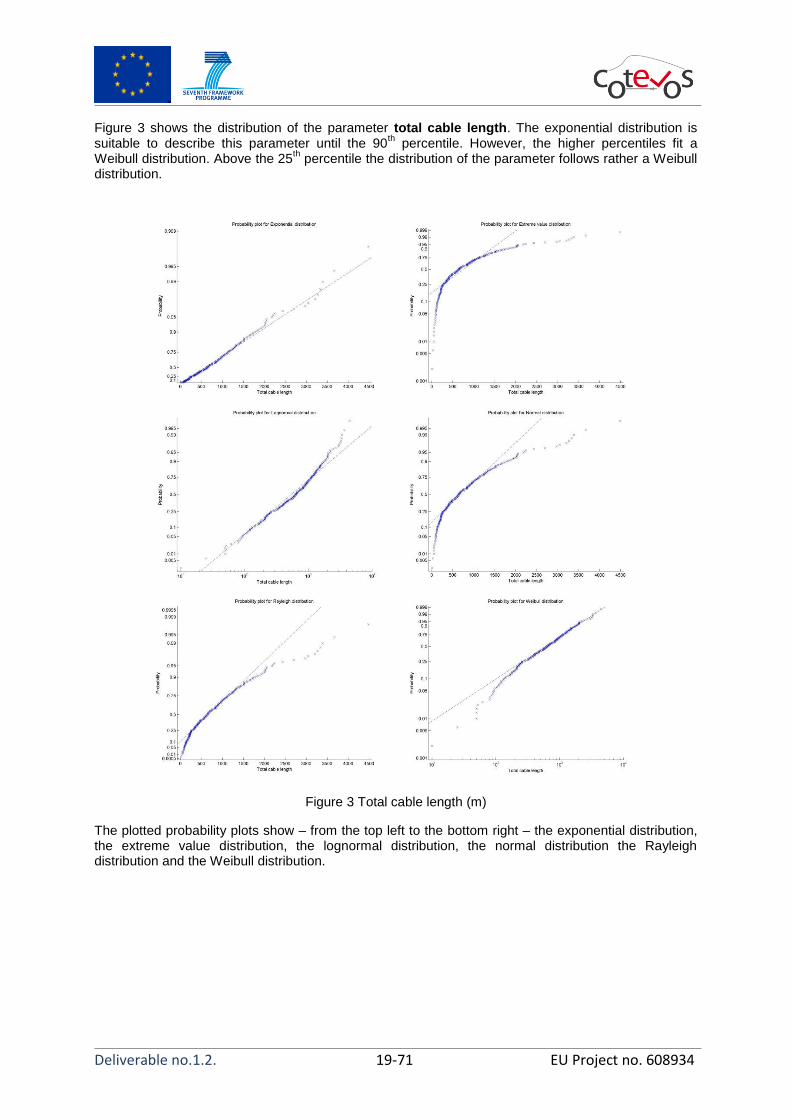
Figure 3 shows the distribution of the parameter total cable length. The exponential distribution is suitable to describe this parameter until the 90
th percentile. However, the higher percentiles fit a
Weibull distribution. Above the 25th percentile the distribution of the parameter follows rather a Weibull
distribution.
Figure 3 Total cable length (m)
The plotted probability plots show – from the top left to the bottom right – the exponential distribution, the extreme value distribution, the lognormal distribution, the normal distribution the Rayleigh distribution and the Weibull distribution.

Deliverable no.1.2. 20-71 EU Project no. 608934
The parameter number of nodes with loads is a discrete distribution. Figure 4 indicates that this parameter cannot be completely explained by any of the 6 distribution functions. However, the Rayleigh distribution shows the lowest error.
Figure 4 Number of nodes with loads (1)
The plotted probability plots show – from the top left to the bottom right – the exponential distribution, the extreme value distribution, the lognormal distribution, the normal distribution the Rayleigh distribution and the Weibull distribution.

Deliverable no.1.2. 21-71 EU Project no. 608934
The next parameter, maximal number of loads (Figure 5) is again a discrete parameter. It is defined by the node in a feeder where the highest number loads are connected to. The figure shows, that the lognormal distribution is the most suitable distribution to explain the parameter.
Figure 5 Maximal number of loads (1)
The plotted probability plots show – from the top left to the bottom right – the exponential distribution, the extreme value distribution, the lognormal distribution, the normal distribution the Rayleigh distribution and the Weibull distribution.

Deliverable no.1.2. 22-71 EU Project no. 608934
The number of cables (Figure 6) in a feeder is again a discrete parameter. It can be explained by either a Rayleigh, Weibull or Extreme value distribution.
Figure 6 Number of cables (1)
The plotted probability plots show – from the top left to the bottom right – the exponential distribution, the extreme value distribution, the lognormal distribution, the normal distribution the Rayleigh distribution and the Weibull distribution.

Deliverable no.1.2. 23-71 EU Project no. 608934
The distribution of the next parameter (number of loads) can be seen in Figure 7. The Exponential distribution shows the least error except one outlier (value 200).
Figure 7 Number of loads (1)
The plotted probability plots show – from the top left to the bottom right – the exponential distribution, the extreme value distribution, the lognormal distribution, the normal distribution the Rayleigh distribution and the Weibull distribution.

Deliverable no.1.2. 24-71 EU Project no. 608934
The behaviour of ratio cables divided by number of nodes with loads (Figure 8) is rather hard to explain according to the considered distributions as it seems not to be following any of the distributions below.
Figure 8 Number of cables divided by number of nodes with loads (1)
The plotted probability plots show – from the top left to the bottom right – the exponential distribution, the extreme value distribution, the lognormal distribution, the normal distribution the Rayleigh distribution and the Weibull distribution.

Deliverable no.1.2. 25-71 EU Project no. 608934
Figure 9 shows the distribution of the reactance of the feeders. The plots show, that the value 0.8Ω can be found at the end node of many feeders. Nevertheless the parameter reactance of the feeder is rather hard to explain. However, among all plots, the lognormal distribution is most suitable to explain this parameter.
Figure 9 Reactance of feeder (Ω/m)
The plotted probability plots show – from the top left to the bottom right – the exponential distribution, the extreme value distribution, the lognormal distribution, the normal distribution the Rayleigh distribution and the Weibull distribution.

Deliverable no.1.2. 26-71 EU Project no. 608934
Figure 10 shows the distribution of the resistance of the feeders. Compared to the reactance, a continuous range can be seen. Beside the exponential distribution, all distributions are suitable to explain this parameter in between the 10
th and 90
th percentile. Lower and upper edges of the range
could be considered as outliers.
Figure 10 Resistance of feeder (Ω/m)
The plotted probability plots show – from the top left to the bottom right – the exponential distribution, the extreme value distribution, the lognormal distribution, the normal distribution the Rayleigh distribution and the Weibull distribution.

Deliverable no.1.2. 27-71 EU Project no. 608934
Figure 11 shows the distribution of a parameter which is the quotient of two parameters, namely the cable length and the number of cables. This parameter therefore describes the average cable length in the feeder. Beside outliers in the upper range of this parameter, the Rayleigh distribution explains this parameter until the 90
th percentile.
Figure 11 Average cable length (m/Cable)
The plotted probability plots show – from the top left to the bottom right – the exponential distribution, the extreme value distribution, the lognormal distribution, the normal distribution the Rayleigh distribution and the Weibull distribution.

Deliverable no.1.2. 28-71 EU Project no. 608934
Figure 12 shows the equivalent reactance of the feeder which is also the quotient of two parameters. It is calculated by the total reactance of the feeder divided by the number of cables. The plots show, that the distributions in the left column are suitable to explain this parameter, where the lognormal distribution is most accurate.
Figure 12 Equivalent reactance (Ω)
The plotted probability plots show – from the top left to the bottom right – the exponential distribution, the extreme value distribution, the lognormal distribution, the normal distribution the Rayleigh distribution and the Weibull distribution.

Deliverable no.1.2. 29-71 EU Project no. 608934
The equivalent resistance (Figure 13), is calculated by the total resistance of the feeder divided by the number of cables. The plots show that the range of this parameter can be explained by all distribution with a specific mismatch, except the extreme value distribution which is not suitable.
Figure 13 Equivalent resistance (Ω)
The plotted probability plots show – from the top left to the bottom right – the exponential distribution, the extreme value distribution, the lognormal distribution, the normal distribution the Rayleigh distribution and the Weibull distribution.

Deliverable no.1.2. 30-71 EU Project no. 608934
Figure 14 shows the ratio of nodes and loads. This parameter is the quotient of the number of nodes divided by the number of loads. The highest value of this parameter is 1, since it described the case where each load is connected to a separate node in the feeder. Below the value 1, the extreme value distribution is suitable to describe this parameter rather well.
Figure 14 Number of nodes divided by number of loads (1)
The plotted probability plots show – from the top left to the bottom right – the exponential distribution, the extreme value distribution, the lognormal distribution, the normal distribution the Rayleigh distribution and the Weibull distribution.

Deliverable no.1.2. 31-71 EU Project no. 608934
Figure 15 shows another combination of parameters, the cable length divided by the number of loads which gives the cable length per load. The upper percentiles are rather hard to describe with the distributions shown in the plots. However, the parameter fits to a normal distribution.
Figure 15 Cable length divided by loads (m/Load)
The plotted probability plots show – from the top left to the bottom right – the exponential distribution, the extreme value distribution, the lognormal distribution, the normal distribution the Rayleigh distribution and the Weibull distribution.

Deliverable no.1.2. 32-71 EU Project no. 608934
Figure 16 shows the distribution of the parameter average distance to neighbour. This parameter is can be explained in a wide range rather by the Rayleigh, lognormal or exponential distribution.
Figure 16 Average distance to neighbours (m)
The plotted probability plots show – from the top left to the bottom right – the exponential distribution, the extreme value distribution, the lognormal distribution, the normal distribution the Rayleigh distribution and the Weibull distribution.

Deliverable no.1.2. 33-71 EU Project no. 608934
Figure 17 shows the distribution of the parameter maximal distance to neighbours in a feeder. The Weibull, lognormal and exponential distributions are suitable to describe this parameter.
Figure 17 Maximal distance to neighbours (m)
The plotted probability plots show – from the top left to the bottom right – the exponential distribution, the extreme value distribution, the lognormal distribution, the normal distribution the Rayleigh distribution and the Weibull distribution.

Deliverable no.1.2. 34-71 EU Project no. 608934
Next, the distribution of the minimal distance to neighbours in the feeders can be seen in Figure 18. The Weibull distribution is most suitable to describe this parameter.
Figure 18 Minimal distance to neighbour (m)
The plotted probability plots show – from the top left to the bottom right – the exponential distribution, the extreme value distribution, the lognormal distribution, the normal distribution the Rayleigh distribution and the Weibull distribution.

Deliverable no.1.2. 35-71 EU Project no. 608934
Figure 19 shows the distribution of the parameter average number of neighbours and indicates the branches in side a feeder. Values higher than two can be explained by alternative supply options (e.g. for maintenance) from neighbouring feeders. The plots show that this parameter is rather hard to describe with the distribution functions. However, the extreme value distribution is capable to describe this parameter in a certain area of range.
Figure 19: Average number of neighbours (m)
The plotted probability plots show – from the top left to the bottom right – the exponential distribution, the extreme value distribution, the lognormal distribution, the normal distribution the Rayleigh distribution and the Weibull distribution.

Deliverable no.1.2. 36-71 EU Project no. 608934
Figure 20 shows the parameter maximal number of neighbours in a feeder. Since it is a discrete number, only integer values can be seen. The integer values can be estimated best by the lognormal distribution.
Figure 20: Maximal number of neighbours (1)
The plotted probability plots show – from the top left to the bottom right – the exponential distribution, the extreme value distribution, the lognormal distribution, the normal distribution the Rayleigh distribution and the Weibull distribution.

Deliverable no.1.2. 37-71 EU Project no. 608934
Figure 21 shows the distribution of the parameter R/X ratio. The Weibull and Rayleigh distribution
show the best fit for this parameter.
Figure 21 R/X ratio

Deliverable no.1.2. 38-71 EU Project no. 608934
Figure 222 shows the highest cable loading during the executed load flow calculation per feeder. Since it is a calculation result, it is not part of the parameters that are used to specify a reference feeder.
Figure 22: Highest cable loading in feeder (%)
The plotted probability plots show – from the top left to the bottom right – the exponential distribution, the extreme value distribution, the lognormal distribution, the normal distribution the Rayleigh distribution and the Weibull distribution.

Deliverable no.1.2. 39-71 EU Project no. 608934
Figure 23 shows the highest voltage during the executed load flow calculation per feeder. Since it is a calculation result, it is not part of the parameters that are used to specify a reference feeder.
Figure 23: Highest voltage in the feeder (p.u.)
The plotted probability plots show – from the top left to the bottom right – the exponential distribution, the extreme value distribution, the lognormal distribution, the normal distribution the Rayleigh distribution and the Weibull distribution.

Deliverable no.1.2. 40-71 EU Project no. 608934
Figure 24 shows the voltage sensitivity on reactive power at the end of the feeder. The parameter can be described either by a lognormal or Rayleigh distribution.
Figure 24 Voltage sensitivity on reactive power at the end node (p.u./MW)
The plotted probability plots show – from the top left to the bottom right – the exponential distribution, the extreme value distribution, the lognormal distribution, the normal distribution the Rayleigh distribution and the Weibull distribution.

Deliverable no.1.2. 41-71 EU Project no. 608934
Figure 25 shows the voltage sensitivity on active power at the end of the feeder. The parameter follows apparently a Weibull distribution. Even though, also a Rayleigh or a lognormal distribution would explain the parameter except the edges.
Figure 25 Voltage sensitivity on active power at the end node (p.u./MW)
The plotted probability plots show – from the top left to the bottom right – the exponential distribution, the extreme value distribution, the lognormal distribution, the normal distribution the Rayleigh distribution and the Weibull distribution.

Deliverable no.1.2. 42-71 EU Project no. 608934
Figure 26 shows the distribution of the short circuit impedance at the end node of the feeders. The figures show, that this parameter fits best the Rayleigh and Weibull distribution.
Figure 26 Short circuit impedance in the feeder (Ω)
The plotted probability plots show – from the top left to the bottom right – the exponential distribution, the extreme value distribution, the lognormal distribution, the normal distribution the Rayleigh distribution and the Weibull distribution.

Deliverable no.1.2. 43-71 EU Project no. 608934
Figure 27 shows the distribution of the short circuit power. The exponential and lognormal distributions show the best fit. The correlation between the short circuit power and the short circuit impedance is direct, therefore only one of these two parameters is needed.
Figure 27 Short circuit power at the end of the feeder (MVA)
The plotted probability plots show – from the top left to the bottom right – the exponential distribution, the extreme value distribution, the lognormal distribution, the normal distribution the Rayleigh distribution and the Weibull distribution.
Deliverable no.1.2. 44-71 EU Project no. 608934
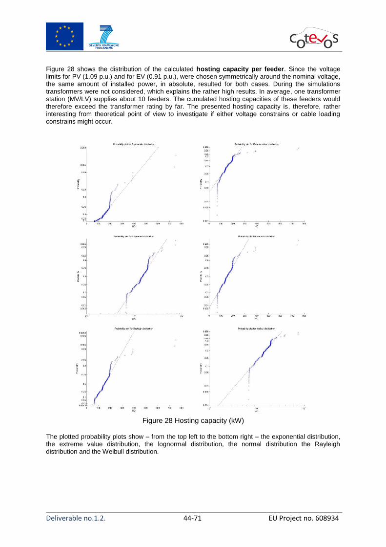
Figure 28 shows the distribution of the calculated hosting capacity per feeder. Since the voltage limits for PV (1.09 p.u.) and for EV (0.91 p.u.), were chosen symmetrically around the nominal voltage, the same amount of installed power, in absolute, resulted for both cases. During the simulations transformers were not considered, which explains the rather high results. In average, one transformer station (MV/LV) supplies about 10 feeders. The cumulated hosting capacities of these feeders would therefore exceed the transformer rating by far. The presented hosting capacity is, therefore, rather interesting from theoretical point of view to investigate if either voltage constrains or cable loading constrains might occur.
Figure 28 Hosting capacity (kW)
The plotted probability plots show – from the top left to the bottom right – the exponential distribution, the extreme value distribution, the lognormal distribution, the normal distribution the Rayleigh distribution and the Weibull distribution.

Deliverable no.1.2. 45-71 EU Project no. 608934
An important result, not visible in Figure 28 is that in a number of feeders both limitation reasons are reached at the same installed power. For example, it should be considered that the reserve in terms of loading could be low in feeders where the voltage limitation occurs before the overloading of cables. Figure 29 shows the investigated feeders. The feeders with a voltage limit are coloured in turquois and feeders with a loading limit in red. Further, the remaining reserve for the opposite limiting factor can be seen. The figure shows that there are a relevant number of feeders where few reserves on the opposite limit are left.
Figure 29 Hosting capacity and reserves
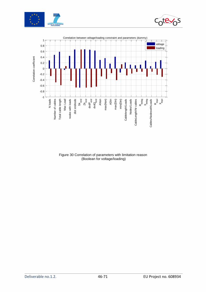
The presented parameters together with the limitation reason (voltage/overloading) were analysed to find which parameter is most promising to estimate the limitation reason.
The limitation reason was converted to a dummy variable (voltage limit reached and loading limit reached). After that, the parameters were correlated with these Boolean variables. Figure 30 shows the spearman correlation of each parameter with the limitation reason for the hosting capacity. The spearman correlation shows the statistical dependence between two variables and thereby assesses how well the relationship between two variables can be described using a monotonic function. It shows, that the usage of dummy variables leads to a rather poor correlation coefficients.
The coefficients increase significantly if the voltage (p.u.) and loading (%) are used instead of Boolean variables. Figure 31 shows that several parameters present a rather high correlation coefficient above 0.8. These parameters are: Distance to end node, short circuit power, short circuit impedance, voltage sensitivity on active power and voltage sensitivity on reactive power.
-1 -0.8 -0.6 -0.4 -0.2 0 0.2 0.4 0.6 0.8 10
100
200
300
400
500
600
700
800
HC-indicator (<0: loading reserve | >0: voltage reserve)
HC
(kW
)
I-limited
U-limited
Deliverable no.1.2. 46-71 EU Project no. 608934
Figure 30 Correlation of parameters with limitation reason (Boolean for voltage/loading)
-1
-0.8
-0.6
-0.4
-0.2
0
0.2
0.4
0.6
0.8
1Correlation between voltage/loading constraint and parameters (dummy)
Corr
ela
tion c
oeff
icie
nt
N loads
Num
ber
of
cable
s
Tota
l cable
length
Max L
oad
nodes w
ith loads
dis
t endnode
Sk
end
Zk e
nd
dvdP
end
dvdQ
end
AN
on
max(N
on)
AD
tn
max(D
tn)
min
(Dtn
)
Cable
length
/Loads
Nodes/L
oads
Cable
Length
/Nr
cable
s
Rbela
g
Xbela
g
Cable
s/N
odesw
ithLoads
Requi
Xequi
voltage
loading

Deliverable no.1.2. 47-71 EU Project no. 608934
Figure 31 Correlation of parameters with voltage and cable loading (p.u. /%)
The parameters most suitable for a classification of networks would be the distance to the end node and the short circuit impedance (or short circuit power). The sensitivity calculations show a little lower correlation coefficient compared to the short circuit impedance. Since the short circuit power and short circuit impedance have a 1/x relation, the short circuit impedance will be used. The remaining parameter distance to end node is rather a topological parameter which is hard to use in a reference grid without any electrical parameters. In summary, the short circuit impedance was selected as suitable parameter. Figure 266 shows that this parameter fits most accurate to a Weibull-distribution. Therefore, the range of the short circuit impedance can be bordered by 0.01Ω and 1Ω, which includes the complete distribution. However, for further analysis, specific percentiles (e.g. 5
th, 50
th and 95
th)
could be selected to investigate the impact of various tests in detail with a reduced number of parameters. The advantage of the parameter short circuit impedance is that the complete network can be reduced and explained by a single value. However, the short circuit impedance has a resistive (R) and reactive (X) part. The ratio R/X itself has a significant impact on the tests. A previous study (morePV2grid) showed that reactive power control strategies could increase the hosting capacity of PV between 20 and 80% depending on the R/X ratio in the feeder. Basically this ratio depends on the cable diameter and the laying system (over-head line or in ground). Since the results of tests could depend on the R/X in the feeder, it is suggested that besides the short circuit impedance, also the R/X ratio should be varied. In the final report of the project morePV2grid, the R/X ratios for in ground cables and overhead-line cables were discussed. For in ground laying R/X ratios between 1.7-7.2 and for over-head lines between 0.8-1.9 were given. Figure 322 shows the R/X ratio at the end node in the investigated feeders which correlates to the previously given ratios [10][12] as well as to the ratios given in D1.2 (e.g Figure 54 or 61).
-1
-0.8
-0.6
-0.4
-0.2
0
0.2
0.4
0.6
0.8
1Correlation between voltage/loading constraint and parameters (p.u./%)
Corr
ela
tion c
oeff
icie
nt
N loads
Num
ber
of
cable
s
Tota
l cable
length
Max L
oad
nodes w
ith loads
dis
t endnode
Sk
end
Zk e
nd
dvdP
end
dvdQ
end
AN
on
max(N
on)
AD
tn
max(D
tn)
min
(Dtn
)
Cable
length
/Loads
Nodes/L
oads
Cable
Length
/Nr
cable
s
Rbela
g
Xbela
g
Cable
s/N
odesw
ithLoads
Requi
Xequi
voltage
loading

Deliverable no.1.2. 48-71 EU Project no. 608934
Figure 32 Distribution of the R/X ratio at the end node of the feeders
The simulations carried out resulted in a hosting capacity per feeder, where either the defined voltage limit (1.09 p.u.) or the cable loading (100%) was reached. Together with the presented parameters a sound environment is available to estimate what kind of limitation will occur first. Figure 333 shows the relation between short circuit impedance and the voltage (left) and the loading (right). The selection of a threshold level for the short circuit impedance shows, that a clear level between feeders with voltage issues and loading issues cannot be drawn. However, if a parameter value of 0.185Ω is chosen, the estimation of the limitation reason is correct for little more than 80% of the feeders.
0.5
1
1.5
2
2.5
3
3.5
4
4.5
5
1
(1)
R/X ratio

Deliverable no.1.2. 49-71 EU Project no. 608934
Figure 33 Short circuit impedance and limitation levels
In conclusion, the variation of the short circuit impedance together with the R/X ratio is suggested. The selection of specific short circuit impedance indicates, with a probability of 80%, which limitation (voltage or loading) could be expected. However, the estimated hosting capacity is rather theoretical. Even though the simulations show that the limitation reason can be estimated, the reached voltage or loading limits might not be reached under real conditions due to other restrictions (e.g. transformer). In the project morePV2grid , during the field tests the voltage remained below a value of 1.06p.u. and the realistic configuration of control strategies (which would start above this level) would not lead to any activation of the control strategies. Therefore the set points had to be reduced to ensure that control strategies act as configured, when necessary [34].
0 0.1 0.2 0.3 0.4 0.5 0.6 0.71
1.02
1.04
1.06
1.08
1.1
1.12
Zk ()
voltage p
.u.
Voltage to short circuit impedance
0 0.1 0.2 0.3 0.4 0.5 0.6 0.730
40
50
60
70
80
90
100
110
Zk ()
cable
loadin
g (
%)
Cable loading to short circuit impedance

Deliverable no.1.2. 50-71 EU Project no. 608934
3. Definition of a reference grid
The COTEVOS reference grid is described as a concept. As a matter of fact the distribution grid landscape of Europe is very diverse. The high amount of distribution networks that are implemented all over Europe reduces the usability and thereby the sense of a single reference grid massively. In the same way that climatic conditions in Europe vary, the grid conditions vary, although in controversy to the climatic conditions, the grid conditions are not based on geographical data. This results in the fact that every EV is much more likely to be exposed to multiple different LV grids than it is to be exposed to very extreme climatic conditions. While only a few people will utilize their EV to cover distances of more than 200-300km and thereby will not occur a dramatic change of climatic conditions, one can easily imagine the example of a person who is charging her/his car in two different distribution grids, e.g. at home and at the working location. The grid interoperability of the EV/EVSE is therefore very important.
Defining a simple reference grid results in a grid that will not be able to cover all the interoperability needs for Europe. One will end up most likely with either a grid that represents an absolute mean value grid, which can be expected to show little to none interoperability issues, or with a grid that describes extreme conditions which will be very specific and thus not of high relevance.
In order to circumvent such a simple and rather useless reference grid for COTEVOS, it was chosen to develop a reference grid parameters table out of which the reference grid can be designed for the specific need of each test case. Utilizing multiple grids for multiple interoperability tests as well as for inter-laboratory comparison is enabled with a low amount of implementation work due to this table.
3.1. Discussion on existing grid types
The very first decision that has to be made when defining a reference grid is the grid topology that will be used. There are multiple grid topologies available, as for example:
3.2. Configuration and operation of LV networks
According to network configuration and operation, LV grid is subdivided as follows: 1. Single fed networks – networks supplied from a single source with no mesh:
a. Simple radial networks; b. Branched radial networks.
2. Bus networks – networks supplied from one or more sources:
a. Loop networks; b. Tree networks; c. Grid networks.
3.2.1. Single fed LV networks
These networks are simple and well-arranged. Each feeder has its own circuit-breaker; the selectivity of the protection level can be achieved by installing fuses with different rated current values. Their main disadvantage is that no substitution is given in case of a failure. Losses are also higher than with bus networks and voltage tends to fluctuate when large consumptions are switched.
1.1. Simple radial networks As shown on Figure 344, these networks have a simple and clear configuration. The main disadvantage is fluctuation of voltage and a low reliability of electricity supply.

Deliverable no.1.2. 51-71 EU Project no. 608934
Figure 34: Simple radial network
1.2. Branched radial networks Branched radial networks are also very simple and well-arranged as it can be seen in Figure 355. The main disadvantage of these networks is also low reliability of electricity supplies.
Figure 35: Branched radial network
Figure 36 shows an example of a network structure in rural area - branched radial networks, where the green part is the LV network and the red part the MV network.

Deliverable no.1.2. 52-71 EU Project no. 608934
Figure 36: Structure of the network in rural area
Figure 377 shows the arrangement of circuit breakers in branched radial networks. The fault current in the fault branch is equal, thus the selectivity of the protection level can be achieved by installing fuses with different rated current values, resulting in different durations of action.
Figure 37: Arrangement of circuit breakers in radial networks

Deliverable no.1.2. 53-71 EU Project no. 608934
2. Bus LV networks Reliability of electricity supplies, as well as higher operation and safety requirements are common for these networks.
2.1. Loop networks As shown in Figure 388, this network is supplied from a single transformer station and forms an enclosed mesh. Loop networks are supplied from two sides. The main advantage of such configuration is that in case of a failure, the switchgear can also be supplied from the other side (in such case, the loop line is divided into two single circuits supplied from one side). The voltage reliability in such networks is higher and when compared to single fed LV networks, losses are also lower. The disadvantage is that higher safety levels are required during work on live lines due to threat of reverse currents caused by supply from both sides.
Figure 38: Loop network
2.2. Tree networks These networks are created when several loop lines are interconnected. This results in a higher level of electricity supply reliability, improved stability of voltage and lower losses. The main disadvantages are that tree networks are complex, complicated and demand higher operational skills.
Figure 39: Tree network
2.3. Grid networks Grid networks are created by linking interconnected networks into meshes. They always have no less than two MV feeders. Out of all network configurations, grid networks provide highest reliability of electricity supplies, lowest possible losses and stable voltage. The entire network is constructed of conductors of an equal cross-section and fuses of an equal rated current are used in all buses of the grid network. The main disadvantage is that these networks are complex, complicated and difficult to operate.

Deliverable no.1.2. 54-71 EU Project no. 608934
Figure 40: Grid network
Figure 411 shows the arrangement of circuit breakers in grid networks. In grid networks, fuses of an equal rated current are used in all buses. Fault current is anyhow divided, thus by means of strength of fault current and subsequent disconnection period, selectivity can be achieved.
Figure 41: Arrangement of circuit breakers in grid network
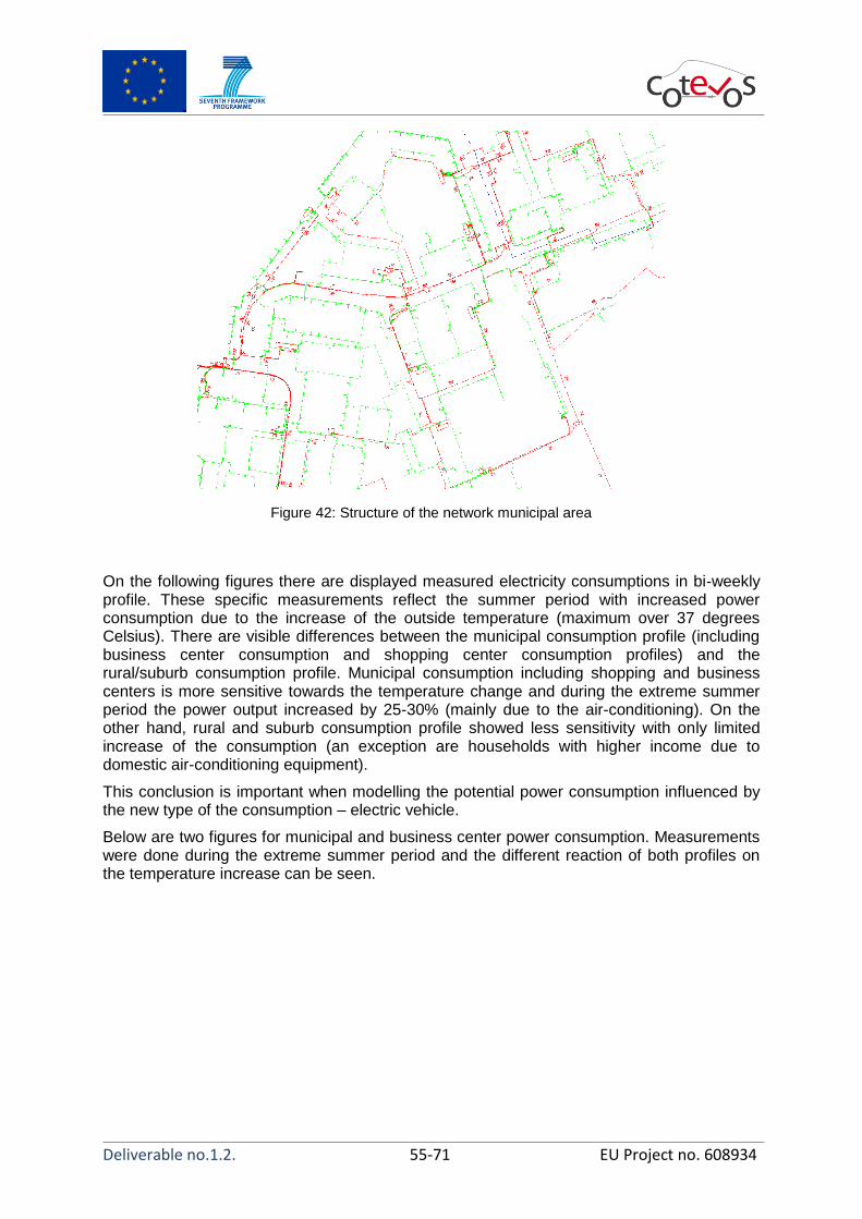
In municipal areas the network structure is more diverse. LV networks (green) are of the bus networks type, red marked are MV cables.
Deliverable no.1.2. 55-71 EU Project no. 608934
Figure 42: Structure of the network municipal area
On the following figures there are displayed measured electricity consumptions in bi-weekly profile. These specific measurements reflect the summer period with increased power consumption due to the increase of the outside temperature (maximum over 37 degrees Celsius). There are visible differences between the municipal consumption profile (including business center consumption and shopping center consumption profiles) and the rural/suburb consumption profile. Municipal consumption including shopping and business centers is more sensitive towards the temperature change and during the extreme summer period the power output increased by 25-30% (mainly due to the air-conditioning). On the other hand, rural and suburb consumption profile showed less sensitivity with only limited increase of the consumption (an exception are households with higher income due to domestic air-conditioning equipment).
This conclusion is important when modelling the potential power consumption influenced by the new type of the consumption – electric vehicle.
Below are two figures for municipal and business center power consumption. Measurements were done during the extreme summer period and the different reaction of both profiles on the temperature increase can be seen.

Deliverable no.1.2. 56-71 EU Project no. 608934
Fig. 10 – typical power consumption of the municipality X axis – date, y axis – power output
Fig. 11 – typical power consumption of the business center object X axis – date, y axis – power output

Deliverable no.1.2. 57-71 EU Project no. 608934
3.3. Discussion on grid development regarding EV/EVSE
In this section a short discussion about the grid development out of the scope of a DSO regarding EV and EVSE is given.
From the DSO point of view the EVs with the charging stations can represent a tool for the grid management. This shift is connected with the responsibility for the deviation transfer, where there is expected extended involvement of the DSOs in the future. DSOs prefer the network regulation execution on the local level, copying the logical structure of the distribution network. Therefore the main component is the regulation on the substation level (22kV/0,4kV).
Any kind of grid regulation is strongly linked with the communication and the access to real data. Bi-directional data flow between EVs, EVSE, back-end system, aggregator/EVSP and SCADA system are the precondition for the utilization of the smart charging. For the communication behind the substation the PLC meets all current requirements. There is a correlation between the SmartMetering concept and e-mobility, as the logic of data gathering is similar. Therefore synergies of both are highly recommended. From the DSO point of view the online access to information on the LV level is the precondition for further smooth integration of charging services (and EVs) and renewable energy sources. In this environment the extension of the SCADA system is the dominant tool.
The EN 50160 standard on the power quality supply is the main framework for DSOs. Moreover it is necessary to link together contracted electricity flows with real electricity flows. Currently the non-predictable renewable energy sources are representing a factor with the highest impact on the real energy flow in the grid.
The EN 50160 power quality standard (Voltage characteristics of electricity supplied by public distribution systems) provides the limits and tolerances of various phenomena that can occur on the mains. Below is a summary of disturbances that are subject of power quality considerations for the low-voltage side of the supply network:
- Grid frequency - Slow voltage changes - Voltage Sags or Dips - Short Interruptions - Accidental, long interruptions - Temporary over-voltages - Transient over-voltages - Voltage unbalance - Harmonic Voltages
The LV network at ZSDis (Slovak DSO) has almost 20 ths km of cables. The absolute dominant portion of customers/off-take points (99,6 %) is connected to the LV network (over 1 mio of off-take points).
At the same time there are limitations imposed by the legislation focusing on the quality of supplied electricity, where the DSO has the responsibility for this measure. If the quality is not adequate, there are financial penalties imposed.
New intermittent/non-predictable electricity generation from renewable energy sources connected mainly to the LV network is changing the situation with the grid management as such. To manage the grid it is important to:
- Clearly identify generation sources at all voltage levels
- On-line measurement of the actual energy flows in the grid (production/consumption)
- On-line measure of network parameters
- Have the option to remotely disconnect a generating source of electricity

Deliverable no.1.2. 58-71 EU Project no. 608934
- Support the security of on-site technicians/maintenance staff
Main challenges linked with the LV network management are:
- Lack of information about real network connections at the local scale
- Insufficient support for the outage management and planned maintenance
- Complicated system support
- Lack of information about connected generation sources
- Integration of data from the Smart Metering
To solve above mentioned challenges it is important to integrate the LV network into the existing SCADA system, with the unified environment for management of all voltage levels – LV, medium-voltage and high-voltage. With this system DSO is able to get up-to-date information from the grid and provide it to the local technician via the mobile SCADA system. The integration with the Smart Metering will lead to the increase of the security for local on-site technicians. At the same time it is necessary to upgrade the existing SCADA system with the incident management module and provide unified system support for the outage management and for planned maintenance.
The only way of sustainable expansion of the distribution grid is the development of applications capable of the autonomous management and operation of the microgrid (local part of the distribution network). Aggregated information are then used for the central grid management – information data set necessary for the microgrid, as follows:
- available power capacity at given time
- free capacity for the electricity distribution
- production and consumption data
- the ability to autonomously identify local outage and separate it from the rest of the grid
3.3.1. Impact of private charging
Home or private charging basic connection represent 16A and 230V parameters, with the theoretical output of 3,7 kW. For this charging process the home installation and local limitations are the basic framework. The charging process is shown on the Figure 433.

Deliverable no.1.2. 59-71 EU Project no. 608934
Figure 43: Domestic charging process (16Ax230V)
On the grid there were no negative impacts of the charging process recorded. Harmonics and Pst are shown in the next table.
Table 2: Harmonics and Pst during a charging process
3.3.2. Impact of fast charging
Fast charger with 50 kW of power output is usually connected to the 22/0.4 kV (630 kVA) substation. Short-circuit power at the point of charger connection is 2.6 MVA. The charging process at the fast charging station is presented on the Figure 444.

Deliverable no.1.2. 60-71 EU Project no. 608934
Figure 44: Charging process at the fast charger
Measurements of the charging process confirmed that the fast charger has the compensation of reactive power. This compensation is designed for compensating of maximum power. Decrease of output power causes decrease of power factor. Problem with reactive power and power factor is considerable in this case and this problem has to be solved, as they enlarge losses and increase costs.
Figure 45: Power Factors (PF) per phase during charging with a charging station X axis – time (t), Y axis – power factor (PF)
In general we can state that the fast charging process does not negatively affect the distribution network. On the other hand there is strong correlation with the quality of the distribution grid and we propose to keep the short-circuit power at least at the level of 0,7 MVA.
200
250
300
350
400
450
500
550
0
10
20
30
40
50
60
70
80
90
10001
:08
00:3
800
:48
00:1
800
:12
00:4
201
:12
01:4
202
:12
02:4
203
:12
03:4
204
:12
04:4
205
:12
05:4
206
:12
06:4
207
:12
07:4
208
:12
08:4
209
:12
09:4
210
:12
10:4
211
:12
11:4
212
:12
12:4
213
:12
13:4
214
:12
14:4
215
:12
15:4
216
:12
16:4
217
:12
17:4
218
:12
18:4
219
:12
19:4
220
:12
20:4
221
:12
21:4
222
:12
22:4
223
:12
23:4
224
:12
24:4
225
:12
25:4
226
:12
26:4
227
:12
27:4
228
:12
28:4
2
Nap
ätie
DC
[V]
Prú
d D
C [
A]
Priebeh napätia a prúdu na strane DC rýchlonabíjacej stanice
prúd DC [A]
napätie DC [V]
Voltage and ampere during charging on the DC site of the charger
Voltage DC (V)
Ampere DC (A)
Vo
lta
ge
DC
(V
)
Am
pe
reD
C (
A)

Deliverable no.1.2. 61-71 EU Project no. 608934
3.3.3. Conclusion
From the DSO perspective the EN 50160 norm is the basic standard which DSO has to comply with. Second precondition is the access to the bi-directional data flow between EV, EVSE, aggregator and SCADA system with the local management possibilities. For further development of the grid it is necessary to enable the autonomous management and operation of the microgrid
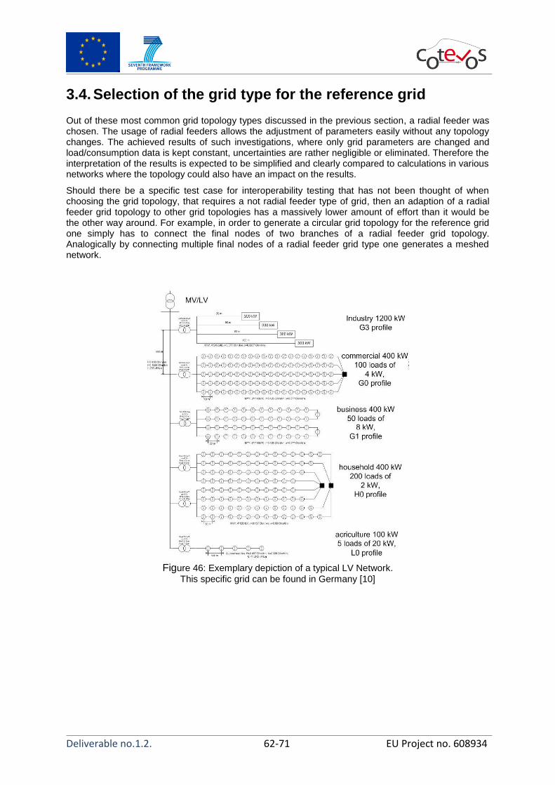
Deliverable no.1.2. 62-71 EU Project no. 608934
3.4. Selection of the grid type for the reference grid
Out of these most common grid topology types discussed in the previous section, a radial feeder was chosen. The usage of radial feeders allows the adjustment of parameters easily without any topology changes. The achieved results of such investigations, where only grid parameters are changed and load/consumption data is kept constant, uncertainties are rather negligible or eliminated. Therefore the interpretation of the results is expected to be simplified and clearly compared to calculations in various networks where the topology could also have an impact on the results.
Should there be a specific test case for interoperability testing that has not been thought of when choosing the grid topology, that requires a not radial feeder type of grid, then an adaption of a radial feeder grid topology to other grid topologies has a massively lower amount of effort than it would be the other way around. For example, in order to generate a circular grid topology for the reference grid one simply has to connect the final nodes of two branches of a radial feeder grid topology. Analogically by connecting multiple final nodes of a radial feeder grid type one generates a meshed network.
Figure 46: Exemplary depiction of a typical LV Network.
This specific grid can be found in Germany [10]

Deliverable no.1.2. 63-71 EU Project no. 608934
Figure 47: Exemplary depiction of a typical LV urban network. This particular grid can be found in Greece [10]
Figure 48: Exemplary depiction of a typical rural LV network. This specific grid can be found in Portugal [35]
Below, Figure 49 presents benchmark LV network model which was developed on the basis of the CIGRE benchmark network which is commonly used for researches on smart grids and RES integration.
The network is supplied by 400kVA distribution transformer, 20/0,4kV. It is common size transformer used in LV urban networks (250 kVA are also common). Three cable feeders deliver energy to three areas: household, industrial and commercial. The first feeder can carry the larges current, 250A per phase, while two next can carry 160A. Some of the loads are supplied directly from the feeder but some of them are supplied via another power lines connected to the feeder. Cables and protection equipment parameters are presented on the scheme.
In the first area (household) we can distinguish two types of loads according to the size: single residential consumers and apartment building. The model assumes that each supplied building ensure for potential EV, at least to the one domestic socket. In case of apartment building the amount of sockets installed e.g. in garage is higher. Similar assumption is made for workshop. In the commercial area there is also access to the socket but there are also charging stations allowing for public charging. There are also distinguished several types of loads.

Deliverable no.1.2. 64-71 EU Project no. 608934
Each load is described on the figure with following information: peak demand value, average demand, number of phases, maximal current (determined by circuit breakers). The AMI represents smart metering device (Advanced Measurement Infrastructure).
Figure 49: Benchmark LV network model developed on the basis of the CIGRE benchmark network
This choice of a radial feeder grid topology for the COTEVOS reference grid is based upon the fact that it is the most common grid topology. In addition in the following main advantages above other grid topologies for a reference grid are given:
Simplification for the implementation
Decreased impact of the grid topology on simulation/emulation results
Increased scalability of the reference grid
Simplified interpretation of results
Increased comparability of results

Deliverable no.1.2. 65-71 EU Project no. 608934
4. Reference grid implementation
4.1. General implementation of a COTEVOS reference grid
The following Table 3Fehler! Verweisquelle konnte nicht gefunden werden. depicts all the parameters that have been evaluated and gives a maximum, a minimum and a mean value for each parameter. Using this table one can assemble the reference grid as needed for the specific test case. Inter-laboratory comparison within the COTEVOS consortium, or other laboratories who commit to the usage of this reference grid parameter set, can thereby be executed, because the parameterization of the reference grid can be transmitted directly and relatively uncomplicated between multiple laboratories. For such a transmission of the reference grid data, only the parameters used as well as the choice of minimum, maximum or mean value have to be communicated. Within Table 3 two parameters have been highlighted. The short circuit impedance (Zk end (Ω) ) and the R/X ratio are considered to be the most important parameters, this follows the conclusion that was
obtained out of Figure 29 to Figure 31.
Table 3: Summary of parameters
Parameter Feeder length
(m) Total cable length
(m) Nodes with loads
(number) Max Load
Number of
cables Number of
loads
min 10.00 10.00 1.00 1.00 1.00 1.00
max 2307.00 4478.00 44.00 45.00 70.00 204.00
avg 430.16 830.82 10.54 5.12 15.78 22.42
distribution Weibull Weibull/Exp Rayleigh Lognormal Rayleigh Exponential
Parameter Cables/Nodes
with Loads R_belag (Ω) X_belag (Ω) CableLength/N
r cables (m) R_equi (Ω) X_equi (Ω)
min 1.00 0.0000 0.0000 10.00 0.0005 0.0002
max 4.00 0.0014 0.0003 888.05 0.1300 0.0304
avg 1.61 0.0005 0.0001 79.88 0.0267 0.0063
distribution Rayleigh
Rayleigh/Lognormal Lognormal Rayleigh Weibull Lognormal
Parameter Nodes/Loads
(number) Cablelength/ Loads
(m) ADtn (m)
max(Dtn) (m)
min(Dtn) (m)
R/X ratio
min 0.04 0.57 4.18 10.00 0.00 0.3720
max 1.00 1776.10 285.00 581.00 190.00 5.1036
avg 0.59 88.98 56.37 135.03 23.34 2.1605
distribution Extreme value Normal lognormal Exponential Weibull Rayleigh
Parameter Anon
max(Non)
dvdP end (p.u./MW)
dvdQ end (p.u./MW)
Sk end (MVA)
Zk end (Ω)
min 1.50 2.00 0.0311 0.0758 0.2965 0.0134
max 2.33 12.00 3.2431 1.9672 12.5252 0.5666
avg 1.89 4.02 0.8654 0.4108 1.6924 0.1584
distribution Extreme value Lognormal Rayleigh Lognormal Exponential Rayleigh

Deliverable no.1.2. 66-71 EU Project no. 608934
Utilizing the parameters given in Table 3 and defining the amount of radial feeders as well as the amount of loads/terminals one can assemble a reference grid as needed for a specific test case in order to test the interoperability behaviour of the EV and the grid all over Europe. A possible implementation of such an interoperability test would be to implement two different reference grids. One being the “worst case scenario type minimum” and the second being the “worst case scenario type maximum”, both utilizing only minimum or maximum values out of the parameter list.
4.2. Exemplary implementation of a COTEVOS reference
grid
Figure 5050 shows exemplarily a reference grid, where a parameter variation was applied per feeder.
The parameters that were adjusted can be seen in Table 4 and were identified as most promising to estimate the reason for the hosting capacity (PV or EV respectively) limitation reason (Overloading or voltage). The nodes were placed equidistant along the feeder and one load per node was placed.
Figure 50: Reference electricity grid example
Table 4: Feeder parameters
Zone Zk (Ω) R/X Feeder length (km)
1 0.320 3.16 1.2
2 0.530 3.912 1.6
3 0.206 2.153 1.2
4 0.052 2.152 0.3
5 0.180 1.588 1.2
6 0.149 0.898 1.6

Deliverable no.1.2. 67-71 EU Project no. 608934
A basic scenario was developed to present the effects of the parameter variation. Per household an electric vehicle charging power of 20 kW (e.g. multi-family house) was assumed and a load flow
calculation was executed. The first voltage column in Table 6 shows the voltages at the nodes in the
reference grid. It can be seen that Zones 1 and 2 are the most effected feeders in the grid. In zone 2 even a voltage drop of nearly 20% can be seen, which indicates that the charging power is not tolerable in this kind of feeders. In a next step, a charging station with reactive power capabilities was assumed to reduce the voltage drop caused by charging. The second voltage column shows the voltage situation in the grid with reactive power provision by each charging station in the households. The comparison of the voltage columns per node shows the voltage gain caused by reactive power. The gain per zone can be seen in Table 4.
Table 5: Impact of reactive power provision (capacitive)
voltage voltage
cos(ϕ)=1 cos(ϕ)= 0.9 cos(ϕ)=1 cos(ϕ)= 0.9
Terminal 1.1 0.958 p.u. 0.964 p.u. Terminal 2.1 0.924 p.u. 0.931 p.u.
Terminal 1.2 0.927 p.u. 0.937 p.u. Terminal 2.2 0.866 p.u. 0.880 p.u.
Terminal 1.3 0.906 p.u. 0.919 p.u. Terminal 2.3 0.827 p.u. 0.845 p.u.
Terminal 1.4 0.895 p.u. 0.910 p.u. Terminal 2.4 0.807 p.u. 0.828 p.u.
Terminal 3.1 0.975 p.u. 0.981 p.u. Terminal 4.1 0.994 p.u. 0.995 p.u.
Terminal 3.2 0.957 p.u. 0.966 p.u. Terminal 4.2 0.990 p.u. 0.992 p.u.
Terminal 3.3 0.944 p.u. 0.956 p.u. Terminal 4.3 0.987 p.u. 0.990 p.u.
Terminal 3.4 0.938 p.u. 0.952 p.u. Terminal 4.4 0.985 p.u. 0.989 p.u.
Terminal 5.1 0.980 p.u. 0.986 p.u. Terminal 6.1 0.987 p.u. 0.994 p.u.
Terminal 5.2 0.965 p.u. 0.975 p.u. Terminal 6.2 0.977 p.u. 0.989 p.u.
Terminal 5.3 0.955 p.u. 0.968 p.u. Terminal 6.3 0.971 p.u. 0.986 p.u.
Terminal 5.4 0.950 p.u. 0.965 p.u. Terminal 6.4 0.968 p.u. 0.985 p.u.
Table 6: voltage reduction per zone
Zone 1 1.5% Zone 2 2.1%
Zone 3 1.4% Zone 4 0.4%
Zone 5 1.5% Zone 6 1. 7%
The example showed, that the reference grid offers a test environment which can be easily parameterized. A parameter variation within the same grid has the advantage that for a specific control strategy (e.g. reactive power provision) the effects can be seen by just one calculation. Further, control strategies could be improved and evaluated with various parameter combinations. Finally, the compact design of the reference grid allows the extension of the network with new feeders in a simple way.

Deliverable no.1.2. 68-71 EU Project no. 608934

Deliverable no.1.2. 69-71 EU Project no. 608934
5. Conclusion
This document reports the COTEVOS approach for a reference grid in order to test grid to EV/EVSE interoperability.
In order to be capable to face the challenge of defining a reference grid that can be utilized to test interoperability between the EV/EVSE and the grid for distribution networks all over Europe it was chosen not to define a single grid but to define a set of parameter values out of which the grid can be composed for adequate testing.
Within Europe there are an enormous number of low voltage distribution grids that any EV/EVSE needs to be interoperable with. In a strong controversy to climatic conditions that depend on geographic positions and are rarely changing within a couple of meters, the conditions of low voltage distribution grids can change within very short distances. In other words it is more likely that an EV will switch low voltage grids with very different behaviour on a daily basis than dramatic changes in climatic conditions are. This underlines the importance of grid-EV/EVSE interoperability.
The COTEVOS approach for a reference grid is based on a unified European mentality derived from the all European COTEVOS mentality. Defining a single reference grid that will be able to cope with the requirements given by all those European low voltage grids is an understandably impossible task. A single grid would most likely be either a grid that defines a “medium” state witch will only rarely result in interoperability issues or a single worst case scenario that is unable to depict other bad grid scenarios and thus cannot be interpreted as representative. In order to cope with this challenge it was chosen not to define a single grid but to provide e methodology that can be utilized in a “close to standardized” way such that multiple interoperability test scenarios can be evaluated with a reasonable afford.
For this provision of methodology a statistical evaluation of the feeders of 34 grids was carried out. This statistical evaluation was based on a set of 24 parameters. These are described within this document. For the choice of the grid topology a radial feeder grid topology was chosen.
Within the final section of this document a reference grid example implementation is provided which can be seen as a “how to use this methodology” guide.
The COTEVOS approach for the reference grid breaks with the traditional approach of providing a single grid but provides a much more versatile and applicable solution for the future of testing grid to EV/EVSE interoperability.

Deliverable no.1.2. 70-71 EU Project no. 608934
6. References
[1] J. Scheffler. Bestimmung der maximal zulssigen Netzanschlussleistung photovoltaischer
Energiewandlungsanlagen in Wohnsiedlungsgebieten, 2002 [2] R. Witzmann, G. Kerber. Aufnahmefähigkeit der Verteilnetze für Strom aus Photovoltaik. ew
Fachthema Erneuerbare Energien, 4:50-54, 2007 [3] R. Witzmann, G. Kerber. Statistische Analyse von NS-Verteilungsnetzen und Modellierung
von Referenznetzen. ew Fachthema Netze, 6:22-26, 2008 [4] C. Kieny et al, Report with the recommendations for grid planning operation, G4V D5.3. v1.9,
05.09.2011 [available: http://www.g4v.eu/downloads.html] [5] Q. Wu, EV portfolio management and impact study, Edison Danish project D2.4, 2.5. & 2.6
v2.0, 22.03.2012 p 48-52 [available: http://www.edison-net.dk/Dissemination/Reports.aspx] [6] M. Ferdowsi, Power Quality Assessment, MERGE D2.3, October 2011 p. 9-14 [available:
http://www.ev-merge.eu/index.php?option=com_content&view=category&layout=blog&id=64&Itemid=53]
[7] R. Cossent, P. Frías, T. Gómez, C. Mateo, Functional Specification for estimating additional investments in distribution networks with high penetration of electric vehicles, MERGE EU project D2.4, 10.01.2011 p.7-19 [available: http://www.ev-merge.eu/index.php?option=com_content&view=category&layout=blog&id=64&Itemid=53]
[8] C. Sánchez et al, Scenarios for the evolution of generation system and transmission, distribution, grid evolution requirements for different scenarios of EV penetration in different countries, MERGE EU project D3.1, 14.02.2011 [available: http://www.ev-merge.eu/index.php?option=com_content&view=category&layout=blog&id=64&Itemid=53]
[9] C. Mateo, P. Frías, Recommendations regarding the best planning practices combined with the most efficient strategies for charging EV to be followed by DSOs, MERGE EU project D4.1., October 2011 [available: http://www.ev-merge.eu/index.php?option=com_content&view=category&layout=blog&id=64&Itemid=53]
[10] C. Schwaegerl, Definition of future Microgrid scenarios and performance indices, More Microgrids EU project DG1, 30.11.2008 [available: http://www.microgrids.eu/documents/666.pdf]
[11] G. Strbac et al., Modelling of microgrid evolution and replacement profiles of EU network infrastructure, More Microgrids EU project DH1, April 2009 [available: http://www.microgrids.eu/documents/676.pdf]
[12] G. Strbac et al., Microgrids in Southern Europe Scenarios: impact studies for typical Greek and Italian distribution networks, More Microgrids EU project H2.B, December 2009 [available: http://www.microgrids.eu/documents/679.pdf]
[13] J. Martí, Physical Demonstrations – fenix project, Stakeholders Advisory Group Presentation, París, 27.05.2009 [available: http://www.fenix-project.org/]
[14] J. Corera, Virtual Power Plant concept in electrical networks, 2nd
International conference on Integration of Renewable and Distributed Energy Resources, December 4-8, Napa, CA, USA [available: http://www.fenix-project.org/]
[15] S. Papathanassiou, N. Hatziargyriou, K. Strunz, A benchmark low voltage microgrid network, Presentation at CIGRE symposium “Power systems with dispersed generation: technologies, impacts on development, operation and performances”, April 2005, Greece
[16] Distribution Test feeders, IEEE PES Distribution System Analysis Subcommittee's Distribution Test Feeder Working Group [online: http://ewh.ieee.org/soc/pes/dsacom/testfeeders/]
[17] Radial Distribution Test feeders, Distribution system analysis subcommittee report [available: http://ewh.ieee.org/soc/pes/dsacom/testfeeders/testfeeders.pdf]
[18] W.H. Kersting, Description of The Comprehensive Distribution Test Feeder, IEEE, July 2010 [online: http://ewh.ieee.org/soc/pes/dsacom/testfeeders/Comprehensive.htm, accessed 03/03/2014]
[19] R.C. Dugan, R.F. Arritt, The IEEE 8500-Node Test Feeder, IEEE PES, April 17, 2010 [available: http://ewh.ieee.org/soc/pes/dsacom/testfeeders/]
[20] R.C. Dugan, S. Carneiro, L. Ramos, D. Penido, Neutral-to-Earth Voltage (NEV) Test Case, IEEE PES Test feeders, April 2010 [available: http://ewh.ieee.org/soc/pes/dsacom/testfeeders/]

Deliverable no.1.2. 71-71 EU Project no. 608934
[21] EPRI Test circuits [online: http://sourceforge.net/p/electricdss/code/HEAD/tree/trunk/Distrib/EPRITestCircuits/, accessed: 03/03/2014]
[22] Taxonomy of prototypical feeders [online: http://sourceforge.net/p/gridlab-d/code/HEAD/tree/, accessed: 03/03/2014]
[23] K.P. Schneider et al., Modern Grid Initiative, Distribution taxonomy final report, PNNL, prepared for US Dep. of Energy, 15/11/2008 [available: http://www.gridlabd.org/models/feeders/taxonomy_of_prototypical_feeders.pdf)
[24] DigSilent Power Factory, weblink, http://www.digsilent.de/index.php/products-powerfactory.html
[25] Mathworks MatLab, weblink, http://www.mathworks.de/products/matlab/ [26] TOR D2 : Richtlinie zur Beurteilung von Netzrückwirkungen, Version 2.1-2013, e-control [27] EN 50160, Voltage characteristics of electricity supplied by public electricity networks, March
2011, CENELEC [28] http://www.mathworks.de/de/help/stats/exponential-distribution.html [29] http://www.mathworks.de/de/help/stats/extreme-value-distribution.html [30] http://www.mathworks.de/de/help/stats/lognormal-distribution.html [31] http://www.itl.nist.gov/div898/handbook/eda/section3/normprpl.htm
[32] Papoulis, Athanasios; Pillai, S. (2001) Probability, Random Variables and Stochastic Process
[33] Corder, G.W. & Foreman, D.I. (2014). Nonparametric Statistics: A Step-by-Step Approach, Wiley. ISBN 978-1118840313.
[34] S. Kadam, B. Bletterie, G. Lauss, C. Winter, M. Heidl, A. Abart: "Evaluation Of Voltage Control Algorithms In Smart Grids: Results Of The Project: Morepv2grid"; 29th European Photovoltaic Solar Energy Conference and Exhibition, Amsterdam; 22.09.2014 - 26.09.2014; in: "EUPVSEC Proceedings", WIP, München Deutschland, (2014), Paper-Nr. 6AV.4.3, 8 S.
[35] C. Kieny et al, Report with the recommendations for grid planning operation, G4V D5.3. v1.9, 05.09.2011 [available: http://www.g4v.eu/downloads.html]
[36] EN 50160 Voltage characteristics of electricity supplied by public distribution systems [37] JANIGA, P.; LIŠKA, M.; JANÍČEK, F.; Influence Electric Vehicle Charging to Power system.
In Electric Power Engineering 2013 : 14th International Scientific Conference. Kouty nad Desnou, Czech Republic, May 28-30, 2013. Ostrava: VŠB - Technical University of Ostrava, 2013, s. 6. ISBN 978-80-248-2988-3
[38]