CONCEPTS, REVIEWS AND SYNTHESES

Costs of predator-induced phenotypic plasticity: a graphicalmodel for predicting the contribution of nonconsumptiveand consumptive effects of predators on prey

Scott D. Peacor • Barbara L. Peckarsky •

Geoffrey C. Trussell • James R. Vonesh

Received: 18 February 2009 / Accepted: 6 June 2012

� Springer-Verlag 2012

Abstract Defensive modifications in prey traits that

reduce predation risk can also have negative effects on prey

fitness. Such nonconsumptive effects (NCEs) of predators

are common, often quite strong, and can even dominate the

net effect of predators. We develop an intuitive graphical

model to identify and explore the conditions promoting

strong NCEs. The model illustrates two conditions neces-

sary and sufficient for large NCEs: (1) trait change has a

large cost, and (2) the benefit of reduced predation out-

weighs the costs, such as reduced growth rate. A corollary

condition is that potential predation in the absence of trait

change must be large. In fact, the sum total of the con-

sumptive effects (CEs) and NCEs may be any value

bounded by the magnitude of the predation rate in the

absence of the trait change. The model further illustrates

how, depending on the effect of increased trait change on

resulting costs and benefits, any combination of strong and

weak NCEs and CEs is possible. The model can also be

used to examine how changes in environmental factors

(e.g., refuge safety) or variation among predator–prey

systems (e.g., different benefits of a prey trait change)

affect NCEs. Results indicate that simple rules of thumb

may not apply; factors that increase the cost of trait change

or that increase the degree to which an animal changes a

trait, can actually cause smaller (rather than larger) NCEs.

We provide examples of how this graphical model can

provide important insights for empirical studies from two

natural systems. Implementation of this approach will

improve our understanding of how and when NCEs are

expected to dominate the total effect of predators. Further,

application of the models will likely promote a better

linkage between experimental and theoretical studies of

NCEs, and foster synthesis across systems.

Keywords Nonlethal effect � Trait-mediated � Phenotypic

plasticity � Nonconsumptive effects � Prey defensive traits

Introduction

Many species adaptively modify their phenotype to reduce

predation risk (Agrawal 2001; Tollrain and Harvell 1999).

Such phenotypic responses of prey to predators are com-

mon across terrestrial, marine, and freshwater systems

(Lima 1998; Tollrain and Harvell 1999; Agrawal 2001) and

include shifts in prey behavior (Resetarits and Wilbur

1991), morphology (Dodson and Havel 1988), develop-

ment (Peckarsky et al. 2002), growth efficiency (McPeek

et al. 2001; Trussell et al. 2006a), and physiology (Creel

et al. 2007). These prey responses often involve trade-offs,

such as reduced growth rate (Abrams 1991a; Werner and

Anholt 1993). Therefore, the direct effects of predators on

prey extend beyond mortality via consumption. Such

Communicated by Craig Osenberg.

S. D. Peacor (&)

Department of Fisheries and Wildlife, Michigan State

University, East Lansing, MI 48824, USA

e-mail: peacor@msu.edu

B. L. Peckarsky

Departments of Zoology and Entomology,

University of Wisconsin, Madison, WI 53706, USA

G. C. Trussell

Marine Science Center, Northeastern University,

430 Nahant Road, Nahant, MA 01908, USA

J. R. Vonesh

Department of Biology, Virginia Commonwealth University,

1000 West Cary Street, P.O. Box 842012, Richmond,

VA 23284, USA

123

Oecologia

DOI 10.1007/s00442-012-2394-9

nonconsumptive predator effects (NCEs), where predators

directly affect prey fitness through induced changes in prey

traits, have been documented for a variety of species and

systems (Peacor and Werner 2004a; Creel et al. 2007). A

better understanding of NCEs is important because NCEs

may be large relative to consumptive predator effects

(reviewed in Peacor and Werner 2004a; Preisser et al.

2005); associated changes in predator–prey functional

responses could strongly influence population and com-

munity dynamics in the short and long term (Abrams 1984,

2010; Bolker et al. 2003; Peacor and Cressler 2012); and

NCEs often initiate indirect effects (i.e. trait-mediated

indirect effects; sensu Abrams et al. 1996) that can strongly

influence community dynamics (Turner and Mittelbach

1990; Wootton 1993; reviewed in Werner and Peacor

2003).

Although there is increasing recognition that NCEs may

influence predator and prey dynamics and have indirect

effects on communities, little attention has been given to

general factors that may affect the relative influence of

NCEs versus consumptive effects (CEs). For example,

large NCEs have been observed in an anuran system

(Peacor and Werner 2001), but it is not known if intrinsic

properties of the anuran species studied, their predators, or

the pond environment explain why NCEs are large in this

system. One notable exception is the work of Schmitz

(2008) showing that the magnitude of NCEs on prey

depends on the foraging mode of predators (e.g., sit-and-

wait vs. active). To understand and predict the influence of

NCEs, a general framework is needed to clarify the char-

acteristics of organisms and environments that affect their

magnitude. Further, because it is likely that the underlying

processes involved in NCEs across systems are analogous,

a framework that identifies the similarities and differences

between systems will help to synthesize the role of NCEs.

Our objective is to develop a general framework (model)

for understanding the conditions that will foster large

NCEs and how changes in the system affect their contri-

bution to the net effect of the predator. NCEs are inherently

complex because multiple factors simultaneously influence

the magnitude of the trait change itself, and how that trait

change affects the fitness of the responding prey. To

accomplish this goal, we develop a graphical model to help

visualize how the processes underlying NCEs interact to

shape their magnitude. We describe the model and examine

how changes in the costs and benefits of the trait change

(due to environmental changes) influence the magnitude of

the optimal trait change and the ensuing NCEs and CEs. In

so doing, the framework elucidates (1) conditions that

foster large trait changes, (2) conditions that foster large

NCEs, (3) the relationship between the magnitude of the

trait change and the NCE, and (4) relationships between the

magnitude of NCEs and CEs.

Materials and methods

General description of the graphical model

We graphically explore the relationship between prey fit-

ness and the magnitude of prey defensive trait change in

response to predation risk (Figs. 1, 2). Fitness is decom-

posed into two broadly defined components: predation rate

and growth rate. Growth rate (solid curves) and predation

rate (dashed curves) are plotted as a function of trait change

(TC). Trait change (on the ordinate) ranges from zero to the

maximum value of the trait change that is set to 1 for

simplicity. An increased trait change in response to pre-

dation risk may represent an increase in the expression of a

trait (or a combination of traits), such as an increase in

spine length, or refuge use, or a decrease in the expression

of a trait, such as reduced swimming speed or time spent

foraging. For simplicity, growth rate is normalized to be

one at zero trait change. Growth rate operationally

encompasses any factors affecting fitness in the absence of

the focal predator, including reproduction and mortality

caused by disease and predators other than the focal

predator. For example, in a simple single predator–single

prey model without NCEs, growth rate using our nomen-

clature would be equal to the growth rate term in a dynamic

growth model and the background mortality (if included).

Predation rate, i.e. probability of death per unit time, is

mortality inflicted by the focal predator.

Decomposing fitness into growth rate and predation rate

enables us to explicitly examine the benefits and costs

associated with trait changes exhibited in response to pre-

dation risk. First, the trait change incurs benefits that occur

through a reduction in the predation rate from the predator,

e.g., by reducing spatial overlap with the predator or

reducing vulnerability due to morphological changes.

Therefore, the predation rate curve (hereafter predation

curve) declines as a function of the trait change. Second,

costs of trait change occur due to inherent tradeoffs asso-

ciated with trait change. We represent the composite effect

of the potential costs to fitness as a negative effect on

growth rate, as represented by a decreasing growth rate

curve (hereafter, growth curve) as a function of the trait

change. Such negative effects that have been measured

empirically include a reduction in somatic growth rate due

to reduced foraging rates or access to resources (reviewed

in Peacor and Werner 2004a), higher susceptibility to other

predators (reviewed in Werner and Peacor 2003), reduced

mating success (Travers and Sih 1991), stress-induced

reduction in fitness (Clinchy et al. 2004), and reduced

fecundity due to suboptimal temperatures due to a micro-

habitat shift (Loose and Dawidowicz 1994).

The magnitudes of NCEs and CEs can be represented

directly with the graphical model. The NCE at any given

Oecologia

123

Fig. 1 Graphical framework examining a linear case: a linear

decrease in growth rate and predation rate with prey defensive trait

change. Growth curves, predation curves, and resultant fitness curves

are represented by solid, dashed, and dotted lines, respectively. a–cThe growth curve is made increasingly steeper representing a higher

cost of a trait change to growth rate, whereas the predation curve is

unchanged. d–f The predation curve is shallower over the same

increasing steeper growth curves, representing less benefit of a trait

change to reduced predation risk. Fitness is defined as the difference

between growth rate and predation rate, with the fitness maximum

corresponding to the optimal trait change (indicated by arrows).The

optimal trait value in the linear case is either 0 (c, e, f) or the

maximum value (set to 1; a, b, d). Nonconsumptive effects (NCEs)

and consumptive effects (CEs) at the optimal trait change are

indicated by black and white bars, respectively, with numbers to theright of the bars representing magnitudes (NCE = 0 if the optimal

trait change is zero as in c, e, and f)

Fig. 2 Graphical framework

examining a nonlinear case: a

linear decrease in growth rate

and accelerating decrease in

predation rates with trait

change. Lines, bars, and arrowsas in Fig. 1. For simplicity of

comparison, growth rate and

predation rate at zero and

maximum (TC = 1) trait

change are the same as in Fig. 1,

and therefore the changes from

left to right and top to bottompanels are identical. b, c, e,

f The predation curve is initially

steeper than the growth curve

leading to an increase in fitness

with trait change, until an

intermediate optimal trait value

is reached where the predation

curve becomes less steep than

the growth curve with

increasing trait change. The

value of the optimal trait change

is indicated below the CE bar

Oecologia

123

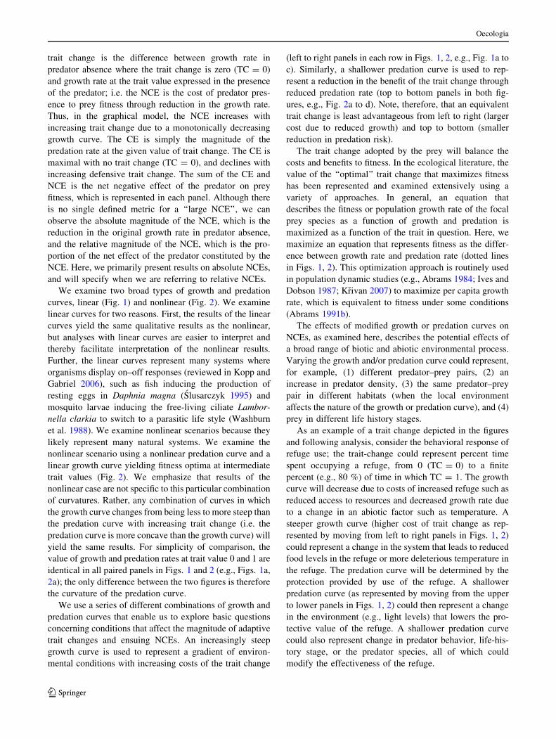
trait change is the difference between growth rate in

predator absence where the trait change is zero (TC = 0)

and growth rate at the trait value expressed in the presence

of the predator; i.e. the NCE is the cost of predator pres-

ence to prey fitness through reduction in the growth rate.

Thus, in the graphical model, the NCE increases with

increasing trait change due to a monotonically decreasing

growth curve. The CE is simply the magnitude of the

predation rate at the given value of trait change. The CE is

maximal with no trait change (TC = 0), and declines with

increasing defensive trait change. The sum of the CE and

NCE is the net negative effect of the predator on prey

fitness, which is represented in each panel. Although there

is no single defined metric for a ‘‘large NCE’’, we can

observe the absolute magnitude of the NCE, which is the

reduction in the original growth rate in predator absence,

and the relative magnitude of the NCE, which is the pro-

portion of the net effect of the predator constituted by the

NCE. Here, we primarily present results on absolute NCEs,

and will specify when we are referring to relative NCEs.

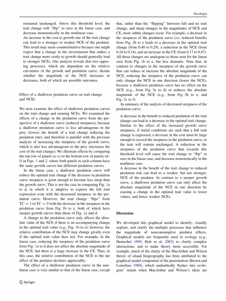
We examine two broad types of growth and predation

curves, linear (Fig. 1) and nonlinear (Fig. 2). We examine

linear curves for two reasons. First, the results of the linear

curves yield the same qualitative results as the nonlinear,

but analyses with linear curves are easier to interpret and

thereby facilitate interpretation of the nonlinear results.

Further, the linear curves represent many systems where

organisms display on–off responses (reviewed in Kopp and

Gabriel 2006), such as fish inducing the production of

resting eggs in Daphnia magna (Slusarczyk 1995) and

mosquito larvae inducing the free-living ciliate Lambor-

nella clarkia to switch to a parasitic life style (Washburn

et al. 1988). We examine nonlinear scenarios because they

likely represent many natural systems. We examine the

nonlinear scenario using a nonlinear predation curve and a

linear growth curve yielding fitness optima at intermediate

trait values (Fig. 2). We emphasize that results of the

nonlinear case are not specific to this particular combination

of curvatures. Rather, any combination of curves in which

the growth curve changes from being less to more steep than

the predation curve with increasing trait change (i.e. the

predation curve is more concave than the growth curve) will

yield the same results. For simplicity of comparison, the

value of growth and predation rates at trait value 0 and 1 are

identical in all paired panels in Figs. 1 and 2 (e.g., Figs. 1a,

2a); the only difference between the two figures is therefore

the curvature of the predation curve.

We use a series of different combinations of growth and

predation curves that enable us to explore basic questions

concerning conditions that affect the magnitude of adaptive

trait changes and ensuing NCEs. An increasingly steep

growth curve is used to represent a gradient of environ-

mental conditions with increasing costs of the trait change

(left to right panels in each row in Figs. 1, 2, e.g., Fig. 1a to

c). Similarly, a shallower predation curve is used to rep-

resent a reduction in the benefit of the trait change through

reduced predation rate (top to bottom panels in both fig-

ures, e.g., Fig. 2a to d). Note, therefore, that an equivalent

trait change is least advantageous from left to right (larger

cost due to reduced growth) and top to bottom (smaller

reduction in predation risk).

The trait change adopted by the prey will balance the

costs and benefits to fitness. In the ecological literature, the

value of the ‘‘optimal’’ trait change that maximizes fitness

has been represented and examined extensively using a

variety of approaches. In general, an equation that

describes the fitness or population growth rate of the focal

prey species as a function of growth and predation is

maximized as a function of the trait in question. Here, we

maximize an equation that represents fitness as the differ-

ence between growth rate and predation rate (dotted lines

in Figs. 1, 2). This optimization approach is routinely used

in population dynamic studies (e.g., Abrams 1984; Ives and

Dobson 1987; Krivan 2007) to maximize per capita growth

rate, which is equivalent to fitness under some conditions

(Abrams 1991b).

The effects of modified growth or predation curves on

NCEs, as examined here, describes the potential effects of

a broad range of biotic and abiotic environmental process.

Varying the growth and/or predation curve could represent,

for example, (1) different predator–prey pairs, (2) an

increase in predator density, (3) the same predator–prey

pair in different habitats (when the local environment

affects the nature of the growth or predation curve), and (4)

prey in different life history stages.

As an example of a trait change depicted in the figures

and following analysis, consider the behavioral response of

refuge use; the trait-change could represent percent time

spent occupying a refuge, from 0 (TC = 0) to a finite

percent (e.g., 80 %) of time in which TC = 1. The growth

curve will decrease due to costs of increased refuge such as

reduced access to resources and decreased growth rate due

to a change in an abiotic factor such as temperature. A

steeper growth curve (higher cost of trait change as rep-

resented by moving from left to right panels in Figs. 1, 2)

could represent a change in the system that leads to reduced

food levels in the refuge or more deleterious temperature in

the refuge. The predation curve will be determined by the

protection provided by use of the refuge. A shallower

predation curve (as represented by moving from the upper

to lower panels in Figs. 1, 2) could then represent a change

in the environment (e.g., light levels) that lowers the pro-

tective value of the refuge. A shallower predation curve

could also represent change in predator behavior, life-his-

tory stage, or the predator species, all of which could

modify the effectiveness of the refuge.

Oecologia

123

In summary, the graphical model explicitly represents

costs and benefits of a trait change. By varying growth and

predation curves, we can examine how different factors

that affect the costs and benefits of trait change influence

the optimal trait change, and the magnitude of NCEs in

predator–prey interactions.

Results

Effects of a steeper growth curve on trait change

and NCEs

Fitness will increase, and thus it is adaptive to express a

larger trait change, when the benefit due to reduced pre-

dation rate outweighs the costs due to reduced growth

rate. In our graphical model, in which fitness is equal to

the difference between predation rate and growth rate,

fitness will therefore increase when the slope of the pre-

dation curve is steeper than that of the growth rate curve.

Consider linear growth and predation curves as depicted

in Fig. 1 in which the predation curve is unchanged, but

the growth curve increases in steepness (from left to right

panels) representing an increased cost of the trait change.

In Fig. 1a, the predation curve is steeper than the growth

curve, and it is adaptive (i.e. fitness is higher) to express

the trait change. In Fig. 1b, the growth curve though

steeper than in Fig. 1a, is still less steep than the preda-

tion curve, and therefore fitness increases as in Fig. 1a

(but less so) with increasing trait change, and it is also

adaptive to express the trait change. In contrast, in

Fig. 1c, the growth curve is steeper than the predation

curve, and it is therefore not adaptive to express the trait

change. Note that if we imagine the steepness of the

growth curve gradually increasing, the adaptive trait

change ‘‘flips’’ from full trait change (Fig. 1a) to no trait

change (Fig. 1c), as found in previous theoretical analyses

examining this linear case (Abrams 1982; Werner and

Anholt 1993).

Consider next the resultant NCEs over the same gradient

of growth curve steepness in the linear case. The initial

increase in steepness represented from Fig. 1a to b is

accompanied by an increase in the NCE. This is because,

even though the optimal trait change is the same (TC = 1),

a steeper growth curve is associated with a higher cost of

the trait change. However, an even steeper growth curve

(Fig. 1c) results in a case where the trait change is no

longer adaptive (TC = 0), so the NCE is also zero. A

continuous increase in the growth curve steepness would

therefore lead to a monotonically increasing value of the

NCE until the NCE falls sharply to zero.

In the nonlinear case, the same processes govern the

optimal trait change, but an intermediate trait change may

be optimal. It is adaptive to express a defensive trait up to

the value at which any additional change will incur a

higher cost (to growth rate) than benefit (to reduced pre-

dation risk). In Fig. 2a, the growth curve is shallower than

the predation curve over the entire trait change range, and

therefore the full trait change (TC = 1) is optimal. In

contrast, in Fig. 2b, the growth curve is initially shallower

than the predation curve, and therefore fitness increases, up

to a certain point, above which the growth curve is pro-

gressively steeper than the predation curve and fitness

declines. There is, therefore, an intermediate optimal trait

value at TC = 0.48. With an even steeper growth curve

(Fig. 2c), the optimal trait change is reached at an even

lower trait change magnitude (TC = 0.32).

Next, consider the effect of the increase in the growth

curve steepness on the NCE in the nonlinear case. The

increase in the steepness of the growth curve from Fig. 2a

to b leads to an increase in the NCE (from 0.05 to 0.24) as a

consequence of two opposing effects. First, the magnitude

of the NCE is higher at any given trait change due to the

increased costs directly associated with a steeper growth

curve. Second, as described above, the increased growth

curve steepness results in a lower optimal trait change,

shifting the NCE to a lower value. This negative shift

reduces the increase in the NCE substantially from what it

would have been if the trait change remained at TC = 1.

These two opposing processes can even lead to a net

reduction of the magnitude of the NCE with increasing

steepness in the growth curve, as exemplified by comparing

Fig. 2e to f where the NCE declines from 0.14 to 0.10 as

the growth curve becomes steeper. Whether the increase in

the steepness of the growth curve increases or decreases,

the magnitude of the NCE depends on the magnitude of the

growth curve change and the relative curvatures of the

growth and predation curves. The opposing two processes

in the nonlinear case are the same two processes operating

in the linear case that led to an increase in the steepness of

the growth curve leading to an increase (Fig. 1a to b) and a

decrease (Fig. 1b to c) in the NCE. In the linear case,

however, the two processes do not oppose each other as in

the nonlinear case, but rather operate separately at different

ranges of the trait change. The linear case, therefore, pro-

vides a simpler illustration of the two processes that can

operate simultaneously in the nonlinear case.

In summary of the analysis of increased steepness of the

growth curve:

An increase in the cost to growth rate of the trait change

can lead to a decrease in the optimal trait change. If

conditions are such that a full trait change is expressed

(Fig. 1a in the linear case or Fig. 2a in nonlinear case),

an increase in the cost must be large enough to exceed

the steepness in the predation curve, or else the trait will

Oecologia

123

remained unchanged. Above this threshold level, the

trait change will ‘‘flip’’ to zero in the linear case, and

decrease monotonically in the nonlinear case.

An increase in the cost to growth rate of the trait change

can lead to a stronger or weaker NCE of the predator.

This result may seem counterintuitive because one might

expect that a change in the environment that makes a

trait change more costly to growth should generally lead

to stronger NCEs. Our analysis reveals that two oppos-

ing processes, which are dependent on the relative

curvatures of the growth and predation curve, dictate

whether the magnitude of the NCE increases or

decreases, both of which are possible outcomes.

Effect of a shallower predation curve on trait change

and NCEs

We next examine the effect of shallower predation curves

on the trait change and ensuing NCEs. We examined the

effects of a change in the predation curve from the per-

spective of a shallower curve (reduced steepness), because

a shallower predation curve is less advantageous to the

prey (lowers the benefit of a trait change reducing the

predation rate), and therefore is parallel with the previous

analysis of increasing the steepness of the growth curve,

which is also less advantageous to the prey (increases the

cost of the trait change). We illustrate effects by comparing

the top row of panels (a–c) to the bottom row of panels (d–

f) in Figs. 1 and 2, where both panels in each column have

the same growth curves but different predation curves.

In the linear case, a shallower predation curve will

reduce the optimal trait change if the decrease in predation

curve steepness is great enough to become less steep than

the growth curve. This is not the case in comparing Fig. 1a

to d, in which it is adaptive to express the full trait

expression even with the decreased steepness in the pre-

dation curve. However, the trait change ‘‘flips’’ form

TC = 1 to TC = 0 with the decrease in the steepness in the

predation curve from Fig. 1b to e, both of which have

steeper growth curves than those of Fig. 1a and d.

A change in the predation curve only affects the abso-

lute value of the NCE if there is an accompanying change

in the optimal trait value (e.g., Fig. 1b to e); however, the

relative contribution of the NCE may change greatly even

if the optimal trait value does not. For example, in the

linear case, reducing the steepness of the predation curve

from Fig. 1a to d does not affect the absolute magnitude of

the NCE, but there is a large increase in the CE. Thus, in

this case, the relative contribution of the NCE to the net

effect of the predator declines appreciably.

The effect of a shallower predation curve in the non-

linear case is very similar to that of the linear case, except

that, rather than the ‘‘flipping’’ between full and no trait

change, and sharp changes in the magnitudes of NCE and

CE, more subtle changes occur. For example, a decrease in

the steepness of the predation curve (i.e. reduced benefit)

from Fig. 2b to e leads to a decrease in the optimal trait

change (from 0.48 to 0.29), a reduction in the NCE (from

0.24 to 0.14), and an increase in the CE (from 0.17 to 0.47).

All these changes are analogous to those seen for the linear

case from Fig. 1b to e, but less dramatic. Note that, in

contrast to changes in the steepness of the growth curve

that can reduce or increase the absolute magnitude of the

NCE, reducing the steepness of the predation curve can

only change the NCE in one direction (lower the NCE),

because a shallower predation curve has no effect on the

NCE (e.g., from Fig. 2a to d) or reduces the absolute

magnitude of the NCE (e.g., from Fig. 2b to e, and

Fig. 2c to f).

In summary of the analysis of decreased steepness of the

predation curve:

A decrease in the benefit to reduced predation of the trait

change can lead to a decrease in the optimal trait change.

Similar to the effect of the increased growth curve

steepness, if initial conditions are such that a full trait

change is expressed, a decrease in the cost must be large

enough to exceed the steepness in the predation curve, or

the trait will remain unchanged. A reduction in the

steepness of the predation curve that exceeds this

threshold level will cause the trait change to ‘‘flip’’ to

zero in the linear case, and decrease monotonically in the

nonlinear case.

A decrease in the benefit of the trait change to reduced

predation risk can lead to a weaker, but not stronger,

NCE of the predator. In contrast to a steeper growth

curve, a shallower predation curve can only affect the

absolute magnitude of the NCE in one direction by

causing a change in the optimal trait value to lower

values, and hence weaker NCEs.

Discussion

We developed this graphical model to identify, visually

explore, and clarify the multiple processes that influence

the magnitude of nonconsumptive predator effects.

Graphical models are frequently used in ecology (e.g.,

Hentschel 1999; Holt et al. 2003) to clarify complex

interactions, and to make theory more accessible. For

example, much of the clarity of the MacArthur and Wilson

theory of island biogeography has been attributed to the

graphical model component of the presentation (Brown and

Lomolino 1989), which undoubtedly flashes into ecolo-

gists’ minds when MacArthur and Wilson’s ideas are

Oecologia

123

referenced. As with island biogeography, our model is

based on theory that can be represented mathematically

(e.g., Abrams 1984; Ives and Dobson 1987; Krivan 2007).

Quantitative predictions require mathematical models and

will be dependent on model specifics such as the optimi-

zation method used. However, the qualitative nature of the

relationships (e.g., growth and predation curves) in this

graphical model enabled us to make the connections to

underlying mechanisms more intuitive and identify coun-

ter-intuitive outcomes.

The analysis of the graphical models clarifies two

intuitive conditions that are necessary and sufficient for the

absolute effect of the NCE to be large:

1. By definition, the growth curve must be steep; i.e.

there must be a large cost to fitness via a reduction in

growth rate caused by a trait change.

2. The predation curve must be steeper than the growth

curve; i.e. benefits of the trait change due to reduced

predation must outweigh costs due to reduced growth

rate. This condition is necessary for a trait change,

which is required for an NCE of any magnitude to

occur.

The combination of a steep growth curve and a preda-

tion curve that is steeper than the growth curve leads to a

corollary condition needed for large NCEs; predation must

be large in the absence of the trait change (i.e. at TC = 0).

Low predation in the absence of trait change sets a narrow

bound on the magnitude of the reduction in growth rate that

would allow for the trait change to be adaptive, thereby

limiting the second condition above, and the potential

magnitude of the NCE. Conversely, if predation is large in

the absence of a trait change (i.e. a potentially voracious

predator), then the trait change response of the prey can be

adaptive even if it incurs a large decrease in growth rate

(e.g., Fig. 1b) and hence leads to a large NCE. Therefore,

the predation rate in the absence of the trait change (i.e. the

maximum potential CE) essentially sets an upper limit on

how large the NCE can be in the presence of a trait change.

This graphical model identified and clarified specific

conditions that affected the absolute magnitude of the

NCE. Whereas defensive trait expression, by definition, is

required for NCEs, factors that influence costs and benefits

that lead to an increase in trait expression do not neces-

sarily cause an increase in the NCE; increased trait

expression may be associated with either an increase (e.g.,

from Fig. 2f to e) or decrease (e.g., Fig. 2e to d) in the

NCE magnitude. We also examined how changes in the

relationships between the costs and benefits of trait

expression affected the magnitude of NCEs. Factors that

reduce the benefit of trait change on predation risk (shal-

lower predation curve) will either have no effect (e.g.,

Fig. 2a to d) or decrease (e.g., Fig. 2b to f) the magnitude

of the NCE. In contrast, a factor that increases the growth

costs of a trait change (increased slope of the growth curve)

can increase (e.g., Fig. 2a to b), have no effect, or decrease

(e.g., Fig. 2e to f) the magnitude of NCEs, depending on

the relative influence of two opposing factors; i.e. the

increased cost at each trait value and a reduced cost asso-

ciated with a reduction in the optimum trait change.

Intuitively, one might expect a positive correlation

between the absolute magnitudes of CEs and NCEs, e.g.,

voracious predators that cause large CEs should also cause

large NCEs. However, our analyses indicate that the

magnitude of the CE and NCE are not necessarily corre-

lated; any combination of large and small CEs and NCEs

are possible. For example, we have presented plausible

scenarios that illustrate trait expression that leads to a large

NCE and CE (Fig. 2c), a large NCE and small CE

(Fig. 1b), a small NCE and large CE (Figs. 1d, 2d, f) and a

small NCE and CE (Figs. 1a, 2a). In essence, the sum total

of the CE and NCE may be any value bounded by the

magnitude of the predation rate in the absence of the trait

change, and the manner in which this sum total is divided

between the NCE and CE is dependent on the form of the

growth and predation curves. In addition, the model does

make one clear prediction between the magnitude of NCEs

and predation risk: NCEs can be large only if the predation

rate is large in the absence of a trait change (as described

above). However, rather than being correlated to the NCE,

predation in the absence of the trait change sets a threshold

for the NCE. This is because a trait change associated with

either a large (Fig. 1b) or a small (Fig. 1a) cost (i.e.

reduction in growth), causing a large and small NCE,

respectively, can be adaptive.

We have focused primarily on the absolute magnitude of

the CE and NCE, which are proportions of the fitness in the

absence of the predator. However, it may be important to

describe the relative magnitudes of the CE and NCE in

some contexts. For example, even if the absolute value of

the NCE is small, the relative contribution of the NCE of a

predator can be large or small. Consider the scenario in

Fig. 2a, in which the absolute magnitude of the NCE and

CE are very small, but their relative contribution is nearly

equal; i.e. the NCE constitutes [50 % of the net effect of

the predator. In this case, the phenotypic response of the

prey to the predator has greatly reduced the net effect of the

predator in such a way that both the NCE and CE con-

tribute a high proportion to the net predator effect. In

contrast, in Fig. 2d, the absolute value of the NCE is also

small, but because of a larger CE, the NCE contributes

more negligibly to the net effect of the predator.

This graphical model can be applied to natural systems

to examine how changes in environmental factors affect

predator–prey interactions within a system or between

systems, or to compare different predator–prey pairs. To do

Oecologia

123

so, estimates must be made of the growth and predation

rate curves as a function of the trait change. Quantifying

those relationships can be difficult, and the degree of dif-

ficulty will vary across systems. Experimental studies

typically measure the effect of predator-induced trait

change on fitness components more amenable to mea-

surement, such as somatic growth rate or percent survival

over a discrete time period. Any negative effect on these

fitness components is presumed to have a negative effect

on long-term demographic parameters. For example, indi-

vidual (somatic) growth rate is predicted to have a large

effect on the fitness of anuran larvae in ephemeral ponds.

In other systems, a well-defined relationship is well

established, such as somatic growth rate in early life his-

tory stages affecting the fitness of Daphnia (Lampert and

Trubetskova 1996). Therefore, our graphical model can be

applied to experimental systems that measure short-term

fitness correlates by, e.g., substituting somatic growth for

growth rate in the model. This application of the model can

provide a road map for studies that examine the contribu-

tion of NCEs in specific natural systems. One can then

develop predictions on how different prey or environ-

mental factors (e.g., water clarity that affects predation

rates or foraging rates, or increased refuge density) will

affect the relative and absolute contribution of the NCE to

the net predator effect. Below, we provide examples of

applications of these graphical models to examine NCEs in

two aquatic systems.

First, we consider the NCEs and CEs of the invasive

predatory cladoceran Bythotrephes on Daphnia mendotae

in Lake Michigan (Pangle et al. 2007). The presence of

Bythotrephes induces Daphnia to migrate to deeper water

that serves as a refuge from predation. Low light levels in

deeper water protect Daphnia from this visual predator but

also lead to reduced fecundity at colder temperatures. We

examined the costs and benefits of this defensive behavior

using data from laboratory experiments. The CE is very

large in the absence of migration, and migration severely

reduces the CE at the cost of a very large NCE, which can

account for as much as 90 % of the net effect of Bytho-

trephes during summer lake conditions (Pangle et al.

2007). This case is most closely represented by Fig. 1b, but

with an even larger cost (NCE). However, if the tempera-

ture gradient is reduced (as occurs in the autumn), the cost

of the behavioral response (growth curve slope) is reduced

with no influence on the benefit (predation curve slope).

This scenario has the same small CE, but the NCE is now

small (similar to Fig. 1a). The relative influence of the

NCE resulting from the same level of vertical migration is

thus strongly dependent on season due to changes in the

vertical temperature gradient. The graphical model

approach can further be used to explore how competition,

other predators, and UV radiation affect the shape of the

growth and predation curves, and consequently influence

the CEs and NCEs of Bythotrephes.

Second, we used the model to predict the optimal

expression of defensive traits, as well as the relative con-

sumptive and nonconsumptive effects of two different

predators on mayflies in Rocky Mountain streams. Baetis

mayflies accelerate their larval development in response to

chemical cues from brook trout (Salvelinus fontinalis), and

thereby reduce their risk of aquatic predation by develop-

ing faster (Peckarsky et al. 2001). Expression of this trait

comes at a fitness cost of *40 % because mayflies meta-

morphose at smaller sizes with reduced fecundity in trout

streams compared to fishless streams where stoneflies are

the top predators (Peckarsky et al. 2002). Brook trout

selectively consume larger-bodied Baetis (Allan 1978), and

the effects of trait change on predation rate can be esti-

mated from previous experiments (McPeek and Peckarsky

1998; McIntosh et al. 2002). In streams with brook trout,

the highest fitness is achieved by expressing the trait

(accelerated development, similar to Fig. 1b, but with

slightly shallower growth and predation curves; Peckarsky

et al. 2008). In fishless streams where stoneflies are the top

predators, Baetis fitness is highest without trait change

(similar to Fig. 1e, but with the entire predation curve

shifted lower; Peckarsky et al. 2008). Application of the

model to this example generated both intuitive and coun-

terintuitive predictions: (1) fitness at optimal trait change is

similar for Baetis in streams with fish or stoneflies as the

top predators, which may explain why those mayflies do

not avoid ovipositing in trout streams (Encalada and

Peckarsky 2006), and is consistent with previous analyses

of probabilities of surviving the larval stage in fish and

fishless streams (Peckarsky et al. 2001); (2) relative and

absolute NCEs are highest with the more voracious pred-

ator (trout), which agrees with previous models (McPeek

and Peckarsky 1998); and (3) net effects on Baetis fitness

by the weaker predator (stoneflies) are due entirely to CEs.

Our analysis examines the direct effects of NCEs and

CEs on fitness as defined by the difference in instantaneous

growth and predation rates. However, direct effects lead to

indirect effects and feedback loops in the system, and

therefore the relative influence of NCEs and CEs can

change through time even in within-generation studies

(Peacor and Werner 2004b). For example, a predator-

induced reduction in prey foraging rate can have a direct

negative effect on prey growth rate, but also indirect

positive effects on prey growth rate (Peacor 2002) through

reduced intra- and interspecific competition, and on

resource abundance (Peacor and Werner 2004b). Spatial

heterogeneity, resource characteristics (e.g., nonlinear

growth), prey density, and the competitor density can all

influence the magnitude of indirect effects, and thereby

affect the sign and magnitude of the net NCE (Relyea

Oecologia

123

2000; Peacor and Werner 2004b; Turner 2004; Trussell

et al. 2006b). In addition, predators may modify hunting

strategy in response to changes in prey traits, adding to the

complexity of the predator–prey interaction (Hugie 2004).

Hence, dynamical models that incorporate indirect effects

and feedback loops are needed to describe how the NCEs on

instantaneous rates described here are expressed over longer

time periods (Bolker et al. 2003; Peacor and Werner 2004b;

Abrams 2010; Peacor and Cressler 2012). Further, over

longer time scales with feedbacks, interactions between the

NCE and CE can arise, such that the net effect of the

predator is the sum of not only the NCE and CE but also of

an interaction between the two (Peacor and Werner 2001).

As mentioned previously, our model is a graphical

representation of previous analytical studies (Abrams 1984;

Ives and Dobson 1987; Krivan 2007) of NCEs, in which

fitness is expressed as the difference in growth rate.

However, this is only one of many different optimization

criteria used by theoreticians to describe the fitness con-

sequences of predator–prey interactions. We performed an

analogous graphical model using the l/g approach to

optimize fitness, which yielded qualitatively similar results.

The well-known l/g rule (where l is mortality rate which

is analogous to our predation rate, and g is growth rate),

which identifies the trait change that maximizes fitness

when l/g is minimized (Gilliam 1982), maximizes fitness

over long time scales, rather than the instantaneous mea-

sure used here. If l/g is used to optimize fitness then

changes in the ratio of l/g must be used to represent fitness

in the graphical model, rather than the difference. We

emphasize that our results can be used to make qualitative

predictions; whereas the optimization method most appli-

cable to a given system and problem would need to be

applied for more quantitative or specific predictions.

Despite their importance to theory, we know very little

about the functional relationships between the costs and

benefits associated with trait change as represented in the

predation and growth curves (Bolker et al. 2003; Abrams

2010; Peacor and Cressler 2012). An exception is theo-

retical work by Werner and Anholt (1993), who used basic

assumptions of predator and prey movement to develop

growth and predation curves to predict predation rate as a

function of prey speed (the trait). Theoretical studies on the

effect of phenotypic responses on population dynamics

have generally assumed functional relationships between

growth and predation rates and trait change. In this study,

we illustrate how the forms of those relationships are

critical to predicting and understanding NCEs, and there-

fore deserve further empirical attention (Bolker et al. 2003;

Peacor and Cressler 2012). We present the graphical model

to help guide empirical work, and facilitate comparison

across systems and the effects of perturbations within

systems.

NCEs are gaining increased attention as an important

component of species interactions affecting species abun-

dances. Although details may vary, the same fundamental

factors are at play in the diverse systems in which they

have been demonstrated. Whereas different species traits

and environmental factors will influence the functional

form of the growth and predation curves that dictate the

magnitude of NCEs, analogous processes determine the

magnitude of trait changes and how trait changes can

influence the outcome of species interactions. To build a

comprehensive understanding of the influence of NCEs and

the factors that affect their magnitude, it will be helpful to

use common frameworks and language in their description.

The graphical model presented here can be used to address

this broad need. The model can be applied to a broad range

of ecological comparisons, including different species

pairs, species characteristics that affect growth rate such as

ontogeny or conditions, density of predators, and envi-

ronmental factors such as temperature and habitat com-

plexity that can affect growth and predation rates. We

encourage empiricists to measure or estimate the growth

and predation curves used in this framework to provide the

much-needed relationships required by ecological theory to

explore general implications of NCEs, not only to prey

population dynamics but also to food web properties such

as stability and resilience.

Acknowledgments This manuscript was improved by constructive

comments on earlier versions from Peter Abrams, Clay Cressler,

Chris Klausmeier, Earl Werner, Scott Creel and his students, Craig

Osenberg, and several anonymous reviewers. This work was con-

ducted as part of the ‘‘Does Fear Matter?’’ Working Group supported

by the National Center for Ecological Analysis and Synthesis, a

Center funded by NSF (Grant #DEB-0072909), the University of

California, and the Santa Barbara Campus. S.D.P. acknowledges

support from NSF grant OCE-0826020 and support from the Michi-

gan Agricultural Experimental Station. J.R.V. acknowledges support

from NSF grant DEB-0717220 and G.C.T. acknowledges NSF grant

OCE-0727628.

References

Abrams PA (1982) Functional responses of optimal foragers. Am Nat

120:382–390

Abrams PA (1984) Foraging time optimization and interactions in

food webs. Am Nat 124:80–96

Abrams PA (1991a) Strengths of indirect effects generated by optimal

foraging. Oikos 62:167–176

Abrams PA (1991b) Life-history and the relationship between food

availability and foraging effort. Ecology 72:1242–1252

Abrams PA (2010) Implications of flexible foraging for interspecific

interactions: lessons from simple models. Funct Ecol 24:7–17

Abrams PA, Menge BA, Mittlebach GG, Spiller D, Yodzis P (1996)

The role of indirect effects in food webs. In: Polis G, Winemiller

K (eds) Food webs: dynamics and structure. Chapman and Hall,

New York, pp 371–395

Agrawal AA (2001) Phenotypic plasticity in the interactions and

evolution of species. Science 294:321–326

Oecologia

123

Allan JD (1978) Trout predation and the size composition of stream

drift. Limnol Oceanogr 23:1231–1237

Bolker B, Holyoak M, Krivan V, Rowe L, Schmitz O (2003)

Connecting theoretical and empirical studies of trait-mediated

interactions. Ecology 84:1101–1114

Brown JH, Lomolino MV (1989) Independent discovery of the

equilibrium theory of island biogeography. Ecology 70:1954–

1957

Clinchy M, Zanette L, Boonstra R, Wingfield JC, Smith JNM (2004)

Balancing food and predator pressure induces chronic stress in

songbirds. Proc R Soc Lond B 271:2473–2479

Creel S, Christianson D, Liley S, Winnie JA (2007) Predation risk

affects reproductive physiology and demography of elk. Science

315:960

Dodson SI, Havel JE (1988) Indirect prey effects: some morpholog-

ical and life history responses of Daphnia pulex exposed to

Notonecta undulata. Limnol Oceanogr 33:1274–1285

Encalada AC, Peckarsky BL (2006) Selective oviposition by the

mayfly Baetis bicaudatus. Oecologia 148:526–537

Gilliam JF (1982). Habitat use and competitive bottlenecks in

size-structured fish populations. PhD thesis, Michigan State

University

Hentschel BT (1999) Complex life cycles in a variable environment:

Predicting when the timing of metamorphosis shifts from

resource dependent to developmentally fixed. Am Nat 154:

549–558

Holt RD, Dobson AP, Begon M, Bowers RG, Schauber EM (2003)

Parasite establishment in host communities. Ecol Lett 6:837–842

Hugie D (2004) A waiting game between black billed plover and its

fiddler crab prey. Anim Behav 67:823–831

Kopp M, Gabriel W (2006) The dynamic effects of an inducible

defense in the Nicholson–Bailey model. Theor Popul Biol 70:

43–55

Krivan V (2007) The Lotka–Volterra predator–prey model with

foraging-predation risk trade-offs. Am Nat 170:771–782

Ives AR, Dobson AP (1987) Antipredator behavior and the population

dynamics of simple predator–prey systems. Am Nat 130:431–

447

Lampert W, Trubetskova I (1996) Juvenile growth rate as a measure

of fitness in Daphnia. Funct Ecol 10:631–635

Lima SL (1998) Stress and decision making under the risk of

predation: recent developments from behavioral, reproductive,

and ecological perspectives. Adv Stud Behav 27:215–290

Loose CJ, Dawidowicz P (1994) Trade-offs in diel vertical migration

by zooplankton—the costs of predator avoidance. Ecology

75:2255–2263

McIntosh AR, Peckarsky BL, Taylor BW (2002) The influence of

predatory fish on mayfly drift: extrapolating from experiments to

nature. Freshw Biol 47:1497–1513

McPeek MA, Grace M, Richardson JML (2001) Physiological and

behavioral responses to predators shape the growth/predation

risk trade-off in damselflies. Ecology 82:1535–1545

McPeek MA, Peckarsky BL (1998) Life histories and the strengths of

species interactions: combining mortality, growth and fecundity

effects. Ecology 79:235–247

Pangle KL, Peacor SD, Johannsson O (2007) Large nonlethal effects

of an invasive invertebrate predator on zooplankton population

growth rate. Ecology 88:402–412

Peacor SD (2002) Positive effect of predators on prey growth rate

through induced modifications of prey behavior. Ecol Lett

5:77–85

Peacor SD, Cressler CE (2012) The implications of adaptive prey

behavior for ecological communities: a review of current theory.

In: Schmitz O, Ohgushi T, Holt RD (eds) Evolution and ecology

of trait-mediated indirect interactions: linking evolution, com-

munity, and ecosystem. Cambridge University Press, Cambrige

(in press)

Peacor SD, Werner EE (2001) The contribution of trait-mediated

indirect effects to the net effects of a predator. Proc Natl Acad

Sci USA 98:3904–3908

Peacor SD, Werner EE (2004a) How dependent are species-pair

interaction strengths on other species in the food web? Ecology

85:2754–2763

Peacor SD, Werner EE (2004b) Context dependence of nonlethal

effects of a predator on prey growth. Israel J Zool 50:139–167

Peckarsky BL, Taylor BW, McIntosh AR, McPeek MA, Lytle DA

(2001) Variation in mayfly size at metamorphosis as a devel-

opmental response to risk of predation. Ecology 82:740–757

Peckarsky BL, McIntosh AR, Taylor BR, Dahl J (2002) Predator

chemicals induce changes in mayfly life history traits: a whole-

stream manipulation. Ecology 83:612–618

Peckarsky BL, Kerans BL, McIntosh AR, Taylor BW (2008) Predator

effects on prey population dynamics in open systems. Oecologia

156:431–440

Preisser EL, Bolnick DI, Benard MF (2005) Scared to death? The

effects of intimidation and consumption in predator–prey

interactions. Ecology 86:501–509

Relyea RA (2000) Trait-mediated indirect effects in larval anurans:

reversing competition with the threat of predation. Ecology

81:2278–2289

Resetarits WJ, Wilbur HM (1991) Choice of oviposition site by Hylachrysoscelis: role of predators and competitors. Ecology 70:220–

228

Schmitz OJ (2008) Effects of predator hunting mode on grassland

ecosystem function. Science 319:952–954

Slusarczyk M (1995) Predator-induced diapause in Daphnia. Ecology

76:1008–1013

Tollrain R, Harvell CD (1999) The ecology and evolution of inducible

defenses. Princeton University Press, Princeton

Travers SE, Sih A (1991) The influence of starvation and predators on

the mating-behavior of a semiaquatic insect. Ecology 72:2123–

2136

Trussell GC, Ewanchuk PJ, Mattassa CM (2006a) The fear of being

eaten reduces energy transfer in a simple food chain. Ecology

87:2979–2984

Trussell GC, Ewanchuk PJ, Matassa CM (2006b) Habitat effects on

the relative importance of trait- and density mediated indirect

interactions. Ecol Lett 9:1245–1252

Turner AM (2004) Non-lethal effects of predators on prey growth

rates depend on prey density and nutrient additions. Oikos 104:

561–569

Turner AM, Mittelbach GG (1990) Predator avoidance and commu-

nity structure—interactions among piscivores, planktivores, and

plankton. Ecology 71:2241–2254

Washburn JO, Gross ME, Mercer DR, Anderson JR (1988) Predator-

induced trophic shift of a free-living ciliate: parasitism of

mosquito larvae by their prey. Science 240:1193–1195

Werner EE, Anholt BR (1993) Ecological consequences of the

tradeoff between growth and mortality rates mediated by

foraging activity. Am Nat 142:242–272

Werner EE, Peacor SD (2003) A review of trait-mediated indirect

interactions. Ecology 84:1083–1100

Wootton JT (1993) Indirect effects and habitat use in an intertidal

community: interaction chains and interaction modifications. Am

Nat 141:71–89

Oecologia

123