cost-sensitive learning and decision making revisited

European Journal of Operational Research 166 (2005) 212–220

www.elsevier.com/locate/dsw

Computing, Artificial Intelligence and Information Technology

Cost-sensitive learning and decision making revisited

Stijn Viaene a,b,*, Guido Dedene a,b

a Department of Applied Economics, Katholieke Universiteit Leuven, Naamsestraat 69, B-3000 Leuven, Belgiumb Vlerick Leuven Gent Management School, Reep 1, B-9000 Gent, Belgium

Received 6 May 2003; accepted 31 March 2004

Available online 24 June 2004

Abstract

In many real-life decision making situations the default assumption of equal misclassification costs underlying pat-

tern recognition techniques is most likely violated. Then, cost-sensitive learning and decision making bring help for

making cost-benefit-wise optimal decisions. This paper brings an up-to-date overview of several methods that aim to

make a broad variety of error-based learners cost-sensitive. More specifically, we revisit direct minimum expected cost

classification, MetaCost, over- and undersampling, and cost-sensitive boosting.

� 2004 Elsevier B.V. All rights reserved.

Keywords: Decision analysis; Cost-sensitive learning; Classification

1. Introduction

Classification techniques are aimed at algorith-

mically learning to allocate data instances,

described as predictor vectors, to predefined in-

stance classes based on a training set of data in-

stances with known class labels. Classification is

one of the foremost learning tasks. One of the

complications that arise when applying theselearning programs in practice, however, is to make

0377-2217/$ - see front matter � 2004 Elsevier B.V. All rights reserv

doi:10.1016/j.ejor.2004.03.031

* Corresponding author. Tel.: +32 16 32 68 91; fax: +32 16

32 67 32.

E-mail address: [email protected] (S.

Viaene).

them reduce the cost of classification rather thanthe error rate, i.e. the percentage of (test) data in-

stances assigned to the wrong class. This is not

unimportant, since in many real-life decision mak-

ing situations the assumption of equal misclassifi-

cation costs, the default operating mode for

many learners, is most likely violated.

Medical diagnosis is a prototypical example.

Here, a false negative prediction, i.e. failing to de-tect a disease, may well have fatal consequences,

whereas a false positive prediction, i.e. diagnosing

a disease for a patient that does not actually have

it, may be less serious. A similar situation arises

for insurance claim fraud detection, where an early

claims screening facility is to help decide upon the

routing of incoming claims through alternative

ed.

mailto:[email protected]

0 0.1 0.2 0.3 0.4 0.5 0.6 0.7 0.8 0.9 10

0.1

0.2

0.3

0.4

0.5

0.6

0.7

0.8

0.9

1

false alarm rate

true

alar

m ra

te

A

C

D

B

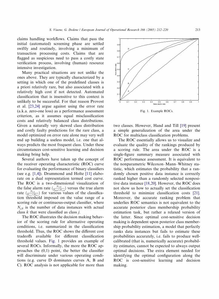
Fig. 1. Example ROCs.

S. Viaene, G. Dedene / European Journal of Operational Research 166 (2005) 212–220 213

claims handling workflows. Claims that pass the

initial (automated) screening phase are settled

swiftly and routinely, involving a minimum of

transaction processing costs. Claims that are

flagged as suspicious need to pass a costly stateverification process, involving (human) resource

intensive investigation.

Many practical situations are not unlike the

ones above. They are typically characterized by a

setting in which one of the predefined classes is

a priori relatively rare, but also associated with a

relatively high cost if not detected. Automated

classification that is insensitive to this context isunlikely to be successful. For that reason Provost

et al. [23,24] argue against using the error rate

(a.k.a. zero-one loss) as a performance assessment

criterion, as it assumes equal misclassification

costs and relatively balanced class distributions.

Given a naturally very skewed class distribution

and costly faulty predictions for the rare class, a

model optimized on error rate alone may very wellend up building a useless model, i.e. one that al-

ways predicts the most frequent class. Under these

circumstances cost-sensitive learning and decision

making bring help.

Several authors have taken up the concept of

the receiver operating characteristic (ROC) curve

for evaluating the performance of binary classifiers

(see e.g. [1,4]). Drummond and Holte [11] elabo-rate on a dual representation termed cost curve.

The ROC is a two-dimensional visualization of

the false alarm rate ð N1;0

N0;0þN1;0Þ versus the true alarm

rate ð N1;1

N1;1þN0;1Þ for various values of the classifica-

tion threshold imposed on the value range of a

scoring rule or continuous-output classifier, where

Nj,k is the number of data instances with actual

class k that were classified as class j.The ROC illustrates the decision making behav-

ior of the scoring rule for alternative operating

conditions, i.e. summarized in the classification

threshold. Thus, the ROC shows the different cost

tradeoffs available for different classification

threshold values. Fig. 1 provides an example of

several ROCs. Informally, the more the ROC ap-

proaches the (0,1) point, the better the classifierwill discriminate under various operating condi-

tions (e.g. curve D dominates curves A, B and

C). ROC analysis is not applicable for more than

two classes. However, Hand and Till [19] present

a simple generalization of the area under the

ROC for multiclass classification problems.

The ROC essentially allows us to visualize and

evaluate the quality of the rankings produced by

a scoring rule. The area under the ROC is a

single-figure summary measure associated withROC performance assessment. It is equivalent to

the nonparametric Wilcoxon–Mann–Whitney sta-

tistic, which estimates the probability that a ran-

domly chosen positive data instance is correctly

ranked higher than a randomly selected nonposi-

tive data instance [18,20]. However, the ROC does

not show us how to actually set the classification

threshold to minimize classification costs [21].Moreover, the accurate ranking problem that

underlies ROC semantics is not equivalent to the

accurate posterior class membership probability

estimation task, but rather a relaxed version of

the latter. Since optimal cost-sensitive decision

making is dependent upon posterior class member-

ship probability estimation, a model that perfectly

ranks data instances but fails to estimate theseprobabilities accurately, i.e. fails to produce well-

calibrated (that is, numerically accurate) probabil-

ity estimates, cannot be expected to always output

optimal decisions. The extra element needed for

identifying the optimal configuration along the

ROC is cost-sensitive learning and decision

making.

214 S. Viaene, G. Dedene / European Journal of Operational Research 166 (2005) 212–220

In this article we revisit several methods for

making classification sensitive to cost asymmetries.

Rather than focus on work gone into making indi-

vidual learners cost-sensitive (see e.g. [3,17]), we

focus on methods that aim to make a broad vari-ety of error-based learners, i.e. learners designed

to minimize error rate and not necessarily generat-

ing models that produce (good) posterior class

probability estimates for the application of mini-

mum expected cost decision making (see Section

2), cost-sensitive. In order of appearance we dis-

cuss: Direct minimum expected cost classification

(Section 2), MetaCost (Section 3), over- and un-dersampling (Section 4) and cost-sensitive boost-

ing (Section 5).

2. Direct minimum expected cost classification

Many classifiers are capable of producing Baye-

sian posterior probability estimates that can beused to classify predictor vectors into the appro-

priate predefined classes. Optimal Bayes decision

making dictates that a predictor vector x 2 Rn

should be assigned to the class t2{1,. . .,T} associ-

ated with the minimum expected cost [12]. Optimal

Bayes assigns classes according to the following

criterion:

argmint2 1;...;Tf g

XTj¼1

p jjxð ÞCt;j xð Þ; ð1Þ

where p(jjx) is the conditional probability of class j

given predictor vector x, and Ct,j(x) is the cost of

classifying a data instance with predictor vectorx and actual class j as class t.

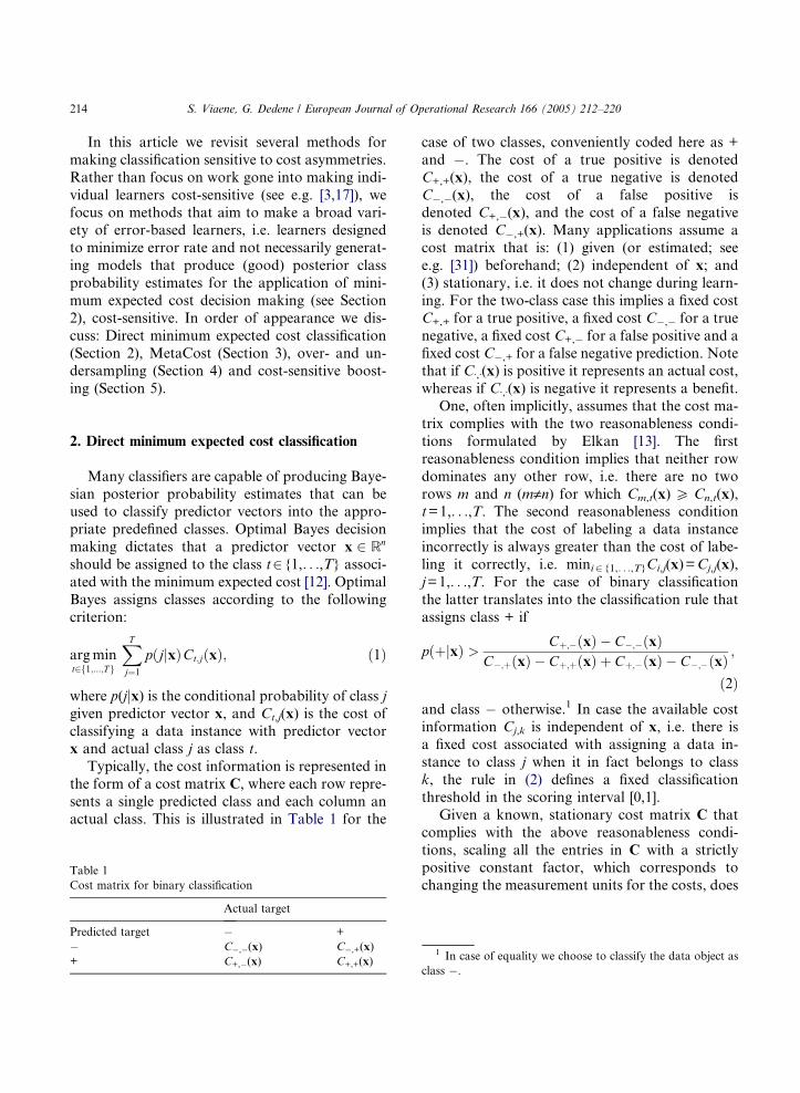
Typically, the cost information is represented in

the form of a cost matrix C, where each row repre-

sents a single predicted class and each column an

actual class. This is illustrated in Table 1 for the

Table 1

Cost matrix for binary classification

Actual target

Predicted target +

C,(x) C,+(x)

+ C+,(x) C+,+(x)

case of two classes, conveniently coded here as +

and . The cost of a true positive is denoted

C+,+(x), the cost of a true negative is denoted

C,(x), the cost of a false positive is

denoted C+,(x), and the cost of a false negativeis denoted C,+(x). Many applications assume a

cost matrix that is: (1) given (or estimated; see

e.g. [31]) beforehand; (2) independent of x; and

(3) stationary, i.e. it does not change during learn-

ing. For the two-class case this implies a fixed cost

C+,+ for a true positive, a fixed cost C, for a true

negative, a fixed cost C+, for a false positive and a

fixed cost C,+ for a false negative prediction. Notethat if CÆ,Æ(x) is positive it represents an actual cost,

whereas if CÆ,Æ(x) is negative it represents a benefit.

One, often implicitly, assumes that the cost ma-

trix complies with the two reasonableness condi-

tions formulated by Elkan [13]. The first

reasonableness condition implies that neither row

dominates any other row, i.e. there are no two

rows m and n (m„n) for which Cm,t(x) P Cn,t(x),t=1,. . .,T. The second reasonableness condition

implies that the cost of labeling a data instance

incorrectly is always greater than the cost of labe-

ling it correctly, i.e. mini2 {1,. . .,T}Ci,j(x)=Cj,j(x),

j=1,. . .,T. For the case of binary classification

the latter translates into the classification rule that

assigns class + if

pðþjxÞ > Cþ;ðxÞ C;ðxÞC;þðxÞ Cþ;þðxÞ þ Cþ;ðxÞ C;ðxÞ

;

ð2Þand class otherwise.1 In case the available costinformation Cj,k is independent of x, i.e. there is

a fixed cost associated with assigning a data in-

stance to class j when it in fact belongs to class

k, the rule in (2) defines a fixed classification

threshold in the scoring interval [0,1].

Given a known, stationary cost matrix C that

complies with the above reasonableness condi-

tions, scaling all the entries in C with a strictlypositive constant factor, which corresponds to

changing the measurement units for the costs, does

1 In case of equality we choose to classify the data object as

class .


not alter the optimal decisions. Moreover, any

such cost matrix C can be transformed into an

equivalent cost matrix C 0 with zero diagonal ele-

ments and positive values for the off-diagonal ele-

ments by adding Cj,j(x) to every column j entryof C, again leaving the optimal classification deci-

sions unaffected [21]. This operation corresponds

to what Elkan [13] calls ‘‘shifting the baseline’’2

for the separate columns of the cost matrix.3

For the minimum expected cost decision mak-

ing criterion in (1) the estimation of p(tjx) is a cru-

cial learning part. An advantage of the direct

application of this decision making scenario is thatit does not require the models to be retrained every

time the costs change, as costs are only introduced

in the post-learning phase. Any error-based classi-

fier that can produce an estimate of p(tjx) can thus

make direct use of (1) to determine the optimal

class. This costing method is termed direct mini-

mum expected cost classification.

Still, the probability estimates output by classi-fiers from many error-based learners are neither

unbiased, nor well-calibrated [32]. Decision tree

learners such as C4.5 and rule learners such as

C4.5rules [25] are well-known examples. They

focus primarily on discrimination between the

classes and only produce posterior class member-

ship probability estimates as a byproduct of classi-

fication. Several methods have been proposed forobtaining better probability estimates from deci-

sion trees and rules. Well-known are smoothing

methods such as Laplace correction and m-estima-

tion smoothing [7,8].

3. MetaCost

MetaCost is aimed at making an error-based

learner cost-sensitive by manipulation of the train-

ing data instance target labels. The learner can be

2 The baseline stands for the starting situation against which

the costs and benefits of the alternative predictions are

evaluated.3 Note that this actually implies that the baseline needs only

to be fixed per column when reasoning on the incurred costs

following a prediction in order to populate the cost matrix

entries.

treated as a black box, requiring no knowledge of

its internals or change to it. The original imple-

mentation of MetaCost due to Domingos [10] is

based on relabeling each training data instance

with its optimal target label according to (1), andthen learning the final classification model using

the relabeled training data. Domingos estimates

p(tjx) using a variant of Breiman�s bagging (boot-

strap aggregation) [5]. MetaCost then works as

follows for training data D ¼ fðxi; tiÞgNi¼1 with

predictor vectors xi 2 Rn and target labels

ti2{1,. . .,T} error-based learner EBL, and cost

matrix C(x):4

(1) Construct internal cost-sensitive classifier

H �ðxÞ : Rn ! f1; . . . ; Tg on D as follows:

(1a) Generate bootstrap resample Dk from D

(Dk having N 06 N data instances), k=1,. . .,K.

(1b) Learn model Hk by applying EBL to Dk,

k=1,. . .,K. Let Hk(x)2{1,. . .,T} denote themodel�s class prediction, and Hk;tðxÞ 2 ½0; 1�denote the model�s confidence in class predic-

tion t given predictor vector x, i.e. its estimate

of p(tjx), only applicable if the model gener-

ated by EBL is able to produce the latter.

(1c) Combine models in (1b) into internal cost-

sensitive classifier H*(x) using minimum ex-

pected cost decision making as follows:

H � xð Þ ¼ argmint2f1;...;Tg

XTj¼1

XKk¼1

hk;j xð ÞCt;j xð Þ; ð3Þ

where hk;jðxÞ ¼ Hk;jðxÞ, if applicable, other-

wise hk,j(x)=1 for j=Hk(x) and hk,j(x)=0 forj „ Hk(x).

(2) Relabel data instances in D using H*(x) to

obtain D*:

D� ¼ xi;H � xið Þð Þf gNi¼1; ð4Þwhere, optionally, the summation over k in (3)

is chosen to range only over those models Hk

for which (xi,ti) 62Dk.

4 MetaCost, as published by Domingos [10], assumes that C

is independent of x. However, nothing precludes MetaCost

from being used with (known) costs Ct,j(x).


(3) Construct final cost-sensitive classifier

HðxÞ : Rn ! f1; . . . ; Tg by applying EBL to

D*.

The MetaCost rationale of constructing a cost-

sensitive classifier H(x) by relabeling the training

data D according to an internal cost-sensitive clas-

sifier H*(x) (step (2)) and reapplying EBL to the

relabeled training data D* (step (3)) can be applied

more generally [29]. We can actually use many

alternative approaches to yield H*(x). For in-stance, instead of using bagging to estimate p(tjx)for applying minimum expected cost decision mak-

ing in step (1) of the original MetaCost, we could

directly use the probability estimates produced by

the model generated by EBL, if these are available.

This implementation was used by Zadrozny and

Elkan [31]. Alternatively, we could use any of the

costing methods described in the following sec-tions for producing H*(x).

An advantage of the MetaCost rationale of re-

labeling the training data is that it produces a single

final model, irrespective of the internal cost-sensi-

tive classifier used. It thus retains the comprehensi-

bility of the models produced by EBL (when they

possess this quality, which e.g. is the case for simple

decision tree and rule learners), while potentiallydrawing upon the strengths of a powerful internal

cost-sensitive classifier (e.g. an ensemble-based

classifier; see Section 5) [9,10].

4. Over- and undersampling

Over- and undersampling are aimed at makingan error-based learner cost-sensitive by manipula-

tion of the training data priors, which are assumed

to be representative of the population priors. They

can be applied for any stationary, instance inde-

pendent (known) two-class cost matrix that com-

plies with the reasonableness conditions specified

in Section 2. We then start from the transformed

cost matrix C 0 as specified in Section 2––specifi-cally, we make use of the off-diagonal elements

of C 0, where we denote the (transformed) cost

for misclassifying a class j data instance as C 0j.

Over- and undersampling cannot, however, be di-

rectly applied for an arbitrary stationary, instance

independent (known) multiclass cost matrix that

complies with the reasonableness conditions speci-

fied in Section 2. Strictly speaking, they are only

applicable to multiclass problems with a particular

type of transformed cost matrix C 0, where we havea constant misclassification cost C 0

j for class j irre-

spective of the predicted class. In other cases, Brei-

man et al. [6] suggest using C0j ¼

Pi2f1;...;Tg:i6¼jC

0i;j;

j ¼ 1; . . . ; T to make the costing method applica-

ble. The rationale underlying changing the training

data priors according to the cost structure is as fol-

lows.

We start from the minimum expected cost deci-sion making criterion, specified as follows:

argmint2 1;...;Tf g

Xj2 1;...;Tf g:j 6¼t

p jjxð ÞC0j: ð5Þ

Using Bayes theorem and noting that p(x) does

not depend on the target label, and therefore does

not affect the classification decision, the criterion

in (5) is rewritten as follows:

argmint2f1;...;Tg

Xj2f1;...;Tg:j 6¼t

pðjÞpðxjjÞC0j: ð6Þ

The decision in (6) can now be reformulated as

follows:

argmint2 1;...;Tf g

Xj2f1;...;Tg:j 6¼t

p0ðjÞpðxjjÞ; ð7Þ

where we specify altered priors p0ðjÞ ¼ pðjÞC0jPT

j¼1pðjÞC0

j

.

The criterion in (7) now suggests that a natural

way to deal with the problem of constant coststructure is to redefine the priors and proceed with

classifier learning as though it were a unit cost

problem [6].

In the undersampling scenario all training data

instances of the class j with the highest p 0(j) are re-

tained and a fraction p0ðiÞp0ðjÞ of the training data in-

stances of each other class i are selected at

random for inclusion in the resampled trainingset. The obvious disadvantage of this scenario is

that it reduces the data available for training,

which may be undesirable. Alternatively, to avoid

the loss of training data, we can apply the over-

sampling scenario, where all training data in-

stances of the class j with the lowest p 0(j) are

retained, and the training data instances of every


other class i are duplicated approximatively p0ðiÞp0ðjÞ

times in the resampled training set [10]. This sce-

nario may, however, seriously increase training

time. Note that some learners can during train-

ing take into account weights specified on thetraining data instances. Resampling of the training

data can then be substituted by reweighting of the

training data instances according to the altered

priors, thus avoiding some of the disadvantages

of resampling. However, when the cost matrix

changes, the costing method will still need to be

reiterated.

5 This choice of ak was derived analytically by Freund and

Shapire [15]. Shapire and Singer [28] leave this choice unspec-

ified and discuss multiple tuning mechanisms.6 Instance weights of less than 108 are automatically set to

108 before normalizing to avoid numerical underflow prob-

lems [2].

5. Cost-sensitive boosting

The mechanics of boosting rest on the construc-

tion of a sequence of classifiers, where each classi-

fier is trained on a resampled (or reweighted, if

applicable) training set where those training data

instances that got poorly predicted in the previousruns receive a higher weight in the next run. At ter-

mination––specifically, after a fixed number of

iterations––the constructed classifiers are then

combined by weighted or simple voting schemes.

The idea underlying the sequential perturbation

of the training data is that the base learner gets

to focus incrementally on those regions of the data

that are harder to learn. For a variety of error-based learners boosting has been reported to re-

duce misclassification error, bias and/or variance

(see e.g. [2,22,27,30]).

In this section we concentrate on the use of

boosting for cost-sensitive classification. We first

describe the boosting algorithm used in this re-

search––specifically, AdaBoost due to Shapire

and Singer [28] designed for two-class problems.Then we present a number of cost-sensitive adap-

tations that have been proposed in the pattern

learning literature for this problem setting.

Following the generalized setting by Shapire

and Singer [28], AdaBoost for a two-class problem

works as follows. For training data D ¼fðxi; tiÞgNi¼1 with predictor vectors xi 2 Rn and tar-

get labels ti2{1,1}, error-based learner EBL, andcost matrix C(x), let the initial instance weights be

w1;i ¼ 1N. Then proceed as follows for run k going

from 1 to K:

(1) Generate data Dk by resampling D using

weights wk,i (Dk having N data instances).

(2) Learn model Hk by applying EBL to Dk. Let

Hk(x)2{1,1} denote the model�s class pre-

diction, and Hk;tðxÞ 2 ½0; 1� denote the mod-el�s confidence in class prediction t given

predictor vector x, i.e. its estimate of p(tjx),only applicable if the model generated by

EBL is able to produce the latter.

(3) Compute ak 2 R as follows:5

ak ¼1

2ln

1þ rk1 rk

� �; ð8Þ

with rk defined as follows:

rk ¼XNi¼1

wk;itihk xið Þ; ð9Þ

where hkðxiÞ ¼ HkðxiÞHk;HkðxiÞðxiÞ, if applica-

ble, otherwise hk(xi)=Hk(x

i).

(4) Update instance weights as follows:

wkþ1;i ¼ wk;i expðaktihkðxiÞÞ: ð10Þ

(5) Normalize wk+1,i by demanding thatPNi¼1wkþ1;i ¼ 1.6

The following final model combination hypoth-

esis HðxÞ : Rn ! f1; 1g is then proposed for clas-

sifying new data instances [28]:

HðxÞ ¼ signXKk¼1

akhkðxÞ !

: ð11Þ

Now we can try to make AdaBoost cost-sensi-

tive. A first way of making AdaBoost cost-sensi-

tive is by replacing (11) with minimum expected

cost decision making. This means that we needto estimate p(tjx). Friedman et al. [16] suggest


passing the real-valued predictions of AdaBoost

through a logistic function to obtain an estimate

of p(t=1jx). That is:

p̂ðt ¼ 1jxÞ ¼ 1

1þ exp PKk¼1

akhkðxÞ� � ; ð12Þ

which is equivalent to interpreting the real-valued

output of AdaBoost as the ln odds of a positive

data instance. The rationale underlying this choice

is the close connection between the exponential cri-

terion that AdaBoost attempts to optimize and the

negative ln likelihood associated with the logisticmodel [26].

A second way to make AdaBoost cost-sensitive

is by using AdaCost, a cost-sensitive variant of

AdaBoost due to Fan et al. [14]. AdaCost uses

the cost of misclassifications to update the training

distribution on successive boosting runs, a costing

method Domingos [10] qualifies as more ad hoc,

lacking clear theoretical foundations for its resam-pling (or reweighting) scheme. AdaCost updates

the instance weights of costly wrong classifications

more aggressively and decreases the weights of

costly correct classifications more conservatively.

To create this effect, AdaCost introduces a cost

adjustment function b(tiHk(xi),ci) in (9) and (10),

with ci 2 Rþ the instance dependent, fixed, nor-

malized7 cost of misclassifying training datainstance (xi,ti). It is assumed that correct classifica-

tions are associated with zero cost. Note that,

given a stationary (known) two-class cost matrix

that is in line with the reasonableness conditions

specified in Section 2, AdaCost�s cost specificationcan always be mimicked by transforming the orig-

inal cost matrix into an equivalent cost matrix with

zero diagonal elements and nonnegative values forthe off-diagonal elements, as described in Section

2. The cost adjustment function is chosen by Fan

et al. [14] as follows: b(1,ci)=0.5ci+0.5 and

b(1,ci)=0.5ci+0.5.

7 AdaCost starts from ci2 [0,1]. Therefore, each cost value is

divided by the maximum cost value.

AdaCost then modifies (9) as follows:

rk ¼XNi¼1

wk;itihkðxiÞbðtiHkðxiÞ; ciÞ: ð13Þ

The weight-update rule in (10) is modified as

follows:

wkþ1;i ¼ wk;i expðaktihkðxiÞbðtiHkðxiÞ; ciÞÞ: ð14ÞFurthermore, the instance weights at run k=1 areset as follows:

w1;i ¼ciPN

i¼1

ci

: ð15Þ

As specified before, some learners can during

training take into account weights specified on the

training data instances. Resampling of the training

data can then be substituted by reweighting of the

training data instances, thus avoiding some of the

disadvantages of resampling. A disadvantage ofAdaCost remains, however, that it requires repeat-

ing all runs every time the costs change, which is not

the case when applying AdaBoost in combination

with minimum expected cost decision making.

Retraining can be a burdensome task. Also, Ada-

Cost, like AdaBoost and other multiple model or

ensemble approaches which can improve signifi-

cantly on the predictive power and stability of singlemodels,8 is not able to retain the comprehensibility

of the models produced by the base learner (when

they possess this quality, which e.g. is the case for

simple decision tree and rule learners) [9].

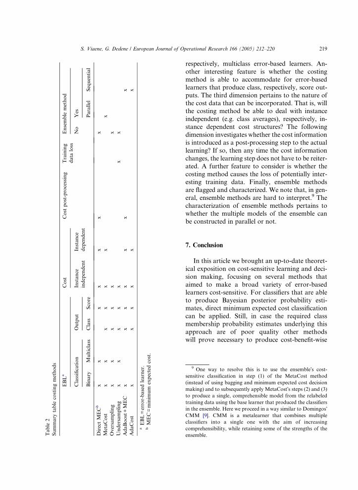
6. Summary

We end this discussion by means of a summary

overview of the main characteristics of each of the

presented costing methods in Table 2. Each of the

discussed costing methods is described along six

dimensions.

The first dimension looked at in Table 2 pertains

to whether the costing method works for binary,

8 For example, decision tree and rule learners are notori-

ously instable, i.e. in the face of limited training data they

produce models that can dramatically change with small

changes in the data [9].

Table

2

Summary

table

costingmethods

EBLa

Cost

Cost

post-processing

Training

data

loss

Ensemble

method

Classification

Output

Instance

independent

Instance

dependent

No

Yes

Binary

Multiclass

Class

Score

Parallel

Sequential

DirectMECb

xx

xx

xx

x

MetaCost

xx

xx

xx

x

Oversampling

xx

xx

xx

Undersampling

xx

xx

xx

x

AdaBoost+MEC

xx

xx

xx

x

AdaCost

xx

xx

xx

aEBL=error-basedlearner.

bMEC=minim

um

expectedcost.


respectively, multiclass error-based learners. An-

other interesting feature is whether the costing

method is able to accommodate for error-based

learners that produce class, respectively, score out-

puts. The third dimension pertains to the nature ofthe cost data that can be incorporated. That is, will

the costing method be able to deal with instance

independent (e.g. class averages), respectively, in-

stance dependent cost structures? The following

dimension investigates whether the cost information

is introduced as a post-processing step to the actual

learning? If so, then any time the cost information

changes, the learning step does not have to be reiter-ated. A further feature to consider is whether the

costing method causes the loss of potentially inter-

esting training data. Finally, ensemble methods

are flagged and characterized. We note that, in gen-

eral, ensemble methods are hard to interpret.9 The

characterization of ensemble methods pertains to

whether the multiple models of the ensemble can

be constructed in parallel or not.

7. Conclusion

In this article we brought an up-to-date theoret-

ical exposition on cost-sensitive learning and deci-

sion making, focusing on several methods that

aimed to make a broad variety of error-basedlearners cost-sensitive. For classifiers that are able

to produce Bayesian posterior probability esti-

mates, direct minimum expected cost classification

can be applied. Still, in case the required class

membership probability estimates underlying this

approach are of poor quality other methods

will prove necessary to produce cost-benefit-wise

9 One way to resolve this is to use the ensemble�s cost-

sensitive classification in step (1) of the MetaCost method

(instead of using bagging and minimum expected cost decision

making) and to subsequently apply MetaCost�s steps (2) and (3)

to produce a single, comprehensible model from the relabeled

training data using the base learner that produced the classifiers

in the ensemble. Here we proceed in a way similar to Domingos�CMM [9]. CMM is a metalearner that combines multiple

classifiers into a single one with the aim of increasing

comprehensibility, while retaining some of the strengths of the

ensemble.


optimal decisions. Thus, we reviewed three alter-

native approaches: MetaCost, over- and under-

sampling, and cost-sensitive boosting.

References

[1] B. Baesens, S. Viaene, D. Van den Poel, J. Vanthienen, G.

Dedene, Bayesian neural network learning for repeat

purchase modelling in direct marketing, European Journal

of Operational Research 138 (1) (2002) 191–211.

[2] E. Bauer, R. Kohavi, An empirical comparison of voting

classification algorithms: Bagging, boosting and variants,

Machine Learning 36 (1–2) (1999) 105–139.

[3] J.P. Bradford, C. Kunz, R. Kohavi, C. Brunk, C.E. Brodley,

Pruning decision trees with misclassification costs, in: Tenth

European Conference on Machine Learning, Chemnitz,

Germany, April 1998.

[4] A.P. Bradley, The use of the area under the ROC curve in

the evaluation of machine learning algorithms, Pattern

Recognition 30 (7) (1997) 1145–1159.

[5] L. Breiman, Bagging predictors, Machine Learning 24 (2)

(1996) 123–140.

[6] L. Breiman, J.H. Friedman, R.A. Olshen, C.J. Stone,

Classification and regression trees (CART), Wadsworth

International Group, Belmont, CA, USA, 1984.

[7] B. Cestnik, Estimating probabilities: A crucial task in

machine learning, in: Ninth European Conference on

Artificial Intelligence, Stockholm, Sweden, August 1990.

[8] J. Cussens. Bayes and pseudo-Bayes estimates of condi-

tional probabilities and their reliability, in: Sixth European

Conference on Machine Learning, Vienna, Austria, April

1993.

[9] P. Domingos, Knowledge discovery via multiple models,

Intelligent Data Analysis 2 (3) (1998) 187–202.

[10] P. Domingos, MetaCost: A general method for making

classifiers cost-sensitive, in: Fifth ACM SIGKDD Interna-

tional Conference on Knowledge Discovery and Data

Mining, San Diego, CA, USA, August 1999.

[11] C. Drummond, R.C. Holte, Explicitly representing ex-

pected cost: An alternative to ROC representation, in:

Sixth ACM SIGKDD International Conference on Knowl-

edge Discovery and Data Mining, Boston, MA, USA,

August 2000.

[12] R.O. Duda, P.E. Hart, D.G. Stork, Pattern Classification,

Wiley, New York, USA, 2000.

[13] C. Elkan, The foundations of cost-sensitive learning, in:

Seventeenth International Joint Conference on Artificial

Intelligence, Seattle, WA, USA, August 2001.

[14] W. Fan, S.J. Stolfo, J. Zhang, P.K. Chan. AdaCost:

Misclassification cost-sensitive boosting, in: Sixteenth

International Conference on Machine Learning, Bled,

Slovenia, June 1999.

[15] Y. Freund, R.E. Shapire, A decision-theoretic generaliza-

tion of on-line learning and an application to boosting,

Journal of Computer and System Sciences 55 (1) (1997)

119–139.

[16] J.H. Friedman, T. Hastie, R. Tibshirani, Additive logistic

regression: A statistical view of boosting, Annals of

Statistics 38 (2) (2000) 337–374.

[17] J. Gama, A cost-sensitive iterative Bayes, in: Seventeenth

International Conference onMachine Learning, Workshop

on Cost-Sensitive Learning, Stanford, CA, USA, June–

July 2000.

[18] D.J. Hand, Construction and Assessment of Classification

Rules, Wiley, Chichester, England, 1997.

[19] D.J. Hand, R.J. Till, A simple generalisation of the area

under the ROC curve for multiple class classification

problems, Machine Learning 45 (2) (2001) 171–186.

[20] J.A. Hanley, B.J. McNeil, The meaning and use of the area

under a receiver operating characteristic (ROC) curve,

Radiology 143 (1) (1982) 29–36.

[21] D.D. Margineantu, Methods for Cost-sensitive Learning,

PhD thesis, Department of Computer Science, Oregon

State University, Corvallis, OR, USA, 2001.

[22] D. Opitz, R. Maclin, Popular ensemble methods: An

empirical study, Journal of Artificial Intelligence Research

11 (1999) 169–198.

[23] F. Provost, T. Fawcett, Robust classification for impre-

cise environments, Machine Learning 42 (3) (2001) 203–

231.

[24] F. Provost, T. Fawcett, R. Kohavi, The case against

accuracy estimation for comparing classifiers, in: Fifteenth

International Conference on Machine Learning, Madison,

WI, USA, July 1998.

[25] J.R. Quinlan, C4.5: Programs for Machine Learning,

Morgan Kaufmann, San Mateo, CA, USA, 1993.

[26] R.E. Schapire, The boosting approach to machine learn-

ing: An overview, in: MSRI Workshop on Nonlinear

Estimation and Classification, Berkeley, CA, USA, March

2002.

[27] R.E. Shapire, Y. Freund, P. Bartlett, W.S. Lee, Boosting

the margin: A new explanation for the effectiveness of

voting methods, Annals of Statistics 26 (5) (1998) 1651–

1686.

[28] R.E. Shapire, Y. Singer, Improved boosting algorithms

using confidence-rated predictions, Machine Learning 37

(3) (1999) 297–336.

[29] K.M. Ting, Z. Zheng, Improving the performance of

boosting for naive Bayesian classification, in: Third Pacific-

Asia Conference on Knowledge Discovery and Data

Mining, Beijing, China, April 1999.

[30] G.I. Webb, MultiBoosting: A technique for combining

boosting and wagging, Machine Learning 40 (2) (2000)

159–196.

[31] B. Zadrozny, C. Elkan, Learning and making decisions

when costs and probabilities are both unknown, in:

Seventh ACM SIGKDD Conference on Knowledge Dis-

covery in Data Mining, San Francisco, CA, USA, August

2001.

[32] B. Zadrozny, C. Elkan, Obtaining calibrated probability

estimates from decision trees and naive Bayesian classifiers,

in: Eighteenth International Conference on Machine

Learning, Williams College, MA, USA, June–July 2001.

cost-sensitive learning and decision making revisited

Documents