cost of saved energy - emp.lbl.gov · the program administrator cost of saved energy for utility...

The Program Administrator Cost of Saved Energy for Utility Customer-Funded Energy Efficiency Programs

Megan A. Billingsley, Ian M. Hoffman, Elizabeth Stuart, Steven R. Schiller, Charles A. Goldman, Kristina LaCommare

Environmental Energy Technologies Division

March 2014

The work described in this report was funded by the National Electricity Delivery Division of the U.S. Department of Energy’s Office of Electricity Delivery and Energy Reliability under Lawrence Berkeley National Laboratory Contract No. DE-AC02-05CH11231.

ERNEST ORLANDO LAWRENCE BERKELEY NATIONAL LABORATORY

LBNL-6595E

The Program Administrator Cost of Energy Saved for Utility Customer-Funded Energy Efficiency Programs

Prepared for the U.S. Department of Energy

National Electricity Delivery Division of the Office of Electricity Delivery and Energy Reliability

Principal Authors

Megan A. Billingsley, Ian M. Hoffman, Elizabeth Stuart, Steven R. Schiller, Charles A. Goldman, Kristina LaCommare

Ernest Orlando Lawrence Berkeley National Laboratory 1 Cyclotron Road, MS 90R4000

Berkeley CA 94720-8136

March 2014

The work described in this report was funded by the National Electricity Delivery Division of the U.S. Department of Energy’s Office of Electricity Delivery and Energy Reliability under Lawrence Berkeley National Laboratory Contract No. DE-AC02-05CH11231.

i

LBNL-6595E

Disclaimer This document was prepared as an account of work sponsored by the United States Government. While this document is believed to contain correct information, neither the United States Government nor any agency thereof, nor The Regents of the University of California, nor any of their employees, makes any warranty, express or implied, or assumes any legal responsibility for the accuracy, completeness, or usefulness of any information, apparatus, product, or process disclosed, or represents that its use would not infringe privately owned rights. Reference herein to any specific commercial product, process, or service by its trade name, trademark, manufacturer, or otherwise, does not necessarily constitute or imply its endorsement, recommendation, or favoring by the United States Government or any agency thereof, or The Regents of the University of California. The views and opinions of authors expressed herein do not necessarily state or reflect those of the United States Government or any agency thereof, or The Regents of the University of California. Ernest Orlando Lawrence Berkeley National Laboratory is an equal opportunity employer.

ii

Acknowledgements

The work described in this report was funded by the National Electricity Delivery Division of the U.S. Department of Energy’s Office of Electricity Delivery and Energy Reliability under Lawrence Berkeley National Laboratory Contract No. DE-AC02-05CH11231. The authors would like to first and foremost thank Larry Mansueti and Cyndy Wilson of the U.S. Department of Energy for their support of this work. We would also like to thank Caitlin Callaghan, Judy Greenwood, George Edgar, Scott Johnstone, Barbara Alexander, Maggie Molina, Tim Woolf, Rich Sedano, Howard Geller, Nick Hall, M. Sami Khawaja, Stan Price, Lara Ettenson, David Goldstein, Peter Miller, Cecily McChalicher, Jim Lazar, Natalie Mims, and Peter Narog for providing comments on a draft of this report. We also thank Anthony Ma for assistance with graphic design and Dana Robson for copyediting. Any remaining omissions and errors are, of course, the responsibility of the authors.

iii

Table of Contents

Acknowledgements ........................................................................................................................ iii

Table of Contents ........................................................................................................................... iv

List of Tables ................................................................................................................................. vi

List of Figures ................................................................................................................................ vi

Acronyms and Abbreviations ...................................................................................................... viii

Executive Summary ....................................................................................................................... ix Results ........................................................................................................................................ xi Observations and Recommendations on Reporting ................................................................. xvi

1. Introduction .................................................................................................................................1 1.1 Assessing Energy Efficiency as a Resource ........................................................................1 1.2 Objectives and Scope ...........................................................................................................2 1.3 Report Organization .............................................................................................................3

2. Approach .....................................................................................................................................4 2.1 Data Summary .....................................................................................................................4 2.2 Program Typology and Standardized Definitions ................................................................7 2.3 Challenges in Consistent and Standardized Reporting of Program Data ..........................11 2.4 Calculating and Using the Cost of Saved Energy ..............................................................12

2.4.1 Levelized Cost of Saved Energy ................................................................................14 2.5 Treatment and Adjustments for Missing Data ...................................................................15

2.5.1 Program Average Measure Lifetime ..........................................................................16 2.5.2 Cost Data for Combined-Fuel Programs....................................................................18 2.5.3 End-Use versus Source and Busbar Energy Savings .................................................18

3. Results—Utility Customer-Funded Programs: Costs and Savings ...........................................19 3.1 Energy Efficiency Program Administrator Expenditures and Savings..............................19

3.1.1 Electric Programs .......................................................................................................19 3.1.2 Gas Program Expenditures and Savings ....................................................................25

3.2 Observations on the Cost of Saved Energy........................................................................27 3.2.1 National Observations ................................................................................................27 3.2.2 Sector and Program Level Observations for Electricity Efficiency Programs ..........30 3.2.3 Regional Observations in Electricity Efficiency Programs .......................................35 3.2.4 Sensitivity Analysis: Impact of Measure Lifetime ....................................................41 3.2.5 Program Administrator and Participant Cost Analysis: The Total Resource Cost of Saved Energy .........................................................................................................................42

4. Testing Influences on the Costs of Saved Energy .....................................................................44 4.1 Hypotheses .........................................................................................................................45 4.2 Approach ............................................................................................................................46 4.3 Preliminary Results: Analysis of Factors that May Influence the Cost of Saved Energy .47

iv

4.3.1 Program Administrator Experience ...........................................................................47 4.3.2 Scale of Program ........................................................................................................48 4.3.3 Labor Costs ................................................................................................................50

4.4 Analytical Challenges ........................................................................................................51

5. Discussion of Key Findings and Recommendations .................................................................52 5.1 Key Findings ......................................................................................................................52 5.2 Discussion: Program Data Collection and Reporting ........................................................54

6. References .................................................................................................................................58

v

List of Tables

Table ES-1. The program administrator cost of saved energy (CSE) for electricity efficiency programs for 2009-2011 data in the LBNL DSM Program Impacts Database (2012$/kWh) .................................................................................................................... xi

Table 2-1. Summary of energy efficiency program data in LBNL DSM Program Impacts Database ............................................................................................................................ 5

Table 2-2. Abridged definitions for selected program cost and savings data ............................... 10 Table 2-3. Program administrator cost of saved energy metrics: definitions and potential uses.. 13 Table 3-1. Program administrator expenditures for 2009–2011 electricity efficiency programs . 20 Table 3-2. U.S. Census Regions and states in the LBNL DSM Program Impacts Database ....... 23 Table 3-3. Program administrator expenditures for 2009-2011 natural gas efficiency programs 26 Table 3-4. The program administrator CSE for electricity efficiency programs by sector: national

savings-weighted averages .............................................................................................. 28 Table 3-5. The program administrator CSE for gas efficiency programs by sector: national

savings-weighted averages ($/therm) .............................................................................. 29 Table 4-1. Factors that may influence the cost of saved energy ................................................... 45

List of Figures

Figure ES-1. CSE for electricity efficiency programs by sector for 2009-2011 data in the LBNL DSM Program Impacts Database .................................................................................... xii

Figure ES-2. National levelized CSE for C&I sector simplified program categories ................. xiii Figure ES-3. National levelized CSE for residential sector simplified program categories ........ xiv Figure ES-4. Levelized savings-weighted average CSE for electricity efficiency programs that

include program administrator costs vs. total resource costs for select program categories ......................................................................................................................................... xv

Figure 2-1. LBNL DSM Program Impacts Database coverage as compared to national efficiency spending reported by Consortium for Energy Efficiency (CEE) ...................................... 6

Figure 2-2. Selected program types in the LBNL program typology ............................................. 8 Figure 2-3. Range of reported program average measure lifetime values for select detailed

program categories .......................................................................................................... 17 Figure 3-1. Program administrator expenditures, first year and lifetime gross savings for 2009–

2011 electricity efficiency programs ............................................................................... 20 Figure 3-2. Program administrator expenditures and lifetime gross savings by simplified program

category for 2009–2011 residential electricity efficiency programs ............................... 21 Figure 3-3. Lifetime gross electricity savings for 2009-2011 residential consumer product rebate

programs .......................................................................................................................... 22 Figure 3-4. Program administrator expenditures and gross lifetime savings for 2009-2011

commercial and industrial electricity efficiency programs ............................................. 23 Figure 3-5. Program administrator expenditures by region for 2009-2011 electricity efficiency

programs .......................................................................................................................... 24 Figure 3-6. Program administrator lifetime savings by region for 2009-2011 electricity efficiency

......................................................................................................................................... 25

vi

Figure 3-7. Program administrator expenditures, first- year and lifetime gross savings for 2009–2011 natural gas efficiency programs ............................................................................. 26

Figure 3-8. National savings-weighted average CSE for electricity efficiency programs by sector ......................................................................................................................................... 28

Figure 3-9. CSE for natural gas efficiency programs by sector .................................................... 30 Figure 3-10. National levelized CSE for electricity efficiency programs by sector ..................... 31 Figure 3-11. National levelized CSE for commercial and industrial sector simplified program

categories ......................................................................................................................... 32 Figure 3-12. National levelized CSE for residential sector simplified program categories ......... 33 Figure 3-13. National levelized CSE for residential whole home detailed program category ..... 34 Figure 3-14. National levelized CSE for residential consumer product rebate detailed program

categories ......................................................................................................................... 35 Figure 3-15. Levelized CSE for electricity efficiency programs by region .................................. 36 Figure 3-16. CSE values by state for electricity efficiency programs (excluding low-income

programs) ......................................................................................................................... 37 Figure 3-17. Percent of regional lifetime savings by climate zone and levelized CSE for

electricity efficiency programs ........................................................................................ 38 Figure 3-18. Levelized CSE for residential new construction programs compared to residential

building energy codes adopted by states in each region ................................................. 39 Figure 3-19. Regional levelized CSEs for commercial new construction programs compared to

commercial building energy codes adopted by states in each region .............................. 40 Figure 3-20. Impact of different program average measure lifetime assumptions on the levelized

CSE for electricity efficiency programs .......................................................................... 42 Figure 3-21. Levelized savings-weighted average CSE for electricity efficiency programs that

include program administrator costs vs. total resource costs for select program categories ......................................................................................................................................... 43

Figure 4-1. First-year portfolio-level CSE and program administrator experience, as measured by years of program spending above a minimal level. ......................................................... 48

Figure 4-2. First-year CSE for appliance recycling programs and the reported number of recycling program participants ........................................................................................ 49

Figure 4-3. First-year portfolio-level CSE values and state average wages for construction industry employees ($/hour) ............................................................................................ 50

Figure 5-1. Components of annual energy efficiency program reporting .................................... 56

vii

Acronyms and Abbreviations

ACEEE American Council for and Energy-efficient Economy C&I commercial and industrial (private sector) CCE Cost of conserved energy CEE Consortium for Energy Efficiency CSE Cost of saved energy DOE U.S. Department of Energy DSM Demand-Side Management EIA Energy Information Administration EERS Energy Efficiency Resource Standards HVAC heating, ventilation, air conditioning LCOE Levelized cost of energy MUSH Municipal and state governments, universities and colleges, K-12 schools, and

healthcare markets WACC Weighted average cost of capital

viii

Executive Summary

End-use energy efficiency is increasingly being relied upon as a resource for meeting electricity and natural gas utility system needs within the United States. There is a direct connection between the maturation of energy efficiency as a resource and the need for consistent, high-quality data and reporting of efficiency program costs and impacts. To support this effort, LBNL initiated the Cost of Saved Energy Project (CSE Project) and created a Demand-Side Management (DSM) Program Impacts Database to provide a resource for policy makers, regulators, and the efficiency industry as a whole.

This study is the first technical report of the LBNL CSE Project and provides an overview of the project scope, approach, and initial findings, including:

• Providing a proof of concept that the program-level cost and savings data can be collected, organized, and analyzed in a systematic fashion;

• Presenting initial program, sector, and portfolio level results for the program administrator CSE for a recent time period (2009-2011); and

• Encouraging state and regional entities to establish common reporting definitions and formats that would make the collection and comparison of CSE data more reliable.

The LBNL DSM Program Impacts Database includes the program results reported to state regulators by more than 100 program administrators in 31 states, primarily for the years 2009–2011. In total, we have compiled cost and energy savings data on more than 1,700 programs over one or more program-years for a total of more than 4,000 program-years’ worth of data, providing a rich dataset for analyses. We use the information to report costs-per-unit of electricity and natural gas savings for utility customer-funded, end-use energy efficiency programs. The program administrator CSE values are presented at national, state, and regional levels by market sector (e.g., commercial, industrial, residential) and by program type (e.g., residential whole home programs, commercial new construction, commercial/industrial custom rebate programs). In this report, the focus is on gross energy savings and the costs borne by the program administrator—including administration, payments to implementation contractors, marketing, incentives to program participants (end users) and both midstream and upstream trade allies, and

Cost of Saved Energy (CSE) vs. Cost Effectiveness

The program administrator’s cost of saved energy is a useful metric for comparing the relative costs of efficiency programs and for comparing an energy efficiency option to other demand and supply choices for serving energy needs. The CSE is comparable to the levelized cost of energy (LCOE), which represents the per-kilowatt hour cost (in real dollars) of building and operating a generating plant over an assumed financial life and duty cycle.

The cost of saved energy is not a direct test of cost effectiveness, however, and is not a benefit-cost analysis, like the Program Administrator’s Cost Test or Utility Cost Test, because it does not purport to capture the monetized value of efficiency to utility customers and shareholders.

ix

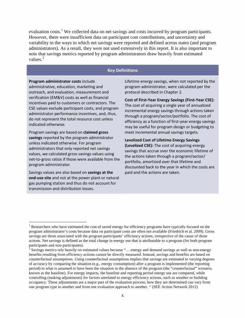
evaluation costs.1 We collected data on net savings and costs incurred by program participants. However, there were insufficient data on participant cost contributions, and uncertainty and variability in the ways in which net savings were reported and defined across states (and program administrators). As a result, they were not used extensively in this report. It is also important to note that savings metrics reported by program administrators draw heavily from estimated values.2

Key Definitions

Program administrator costs include administrative, education, marketing and outreach, and evaluation, measurement and verification (EM&V) costs as well as financial incentives paid to customers or contractors. The CSE values exclude participant costs, and program administrator performance incentives, and, thus, do not represent the total resource cost unless indicated otherwise.

Program savings are based on claimed gross savings reported by the program administrator unless indicated otherwise. For program administrators that only reported net savings values, we calculated gross savings values using net-to-gross ratios if those were available from the program administrator.

Savings values are also based on savings at the end-use site and not at the power plant or natural gas pumping station and thus do not account for transmission and distribution losses.

Lifetime energy savings, when not reported by the program administrator, were calculated per the protocol described in Chapter 2.

Cost of First-Year Energy Savings (First-Year CSE): The cost of acquiring a single year of annualized incremental energy savings through actions taken through a program/sector/portfolio. The cost of efficiency as a function of first-year energy savings may be useful for program design or budgeting to meet incremental annual savings targets.

Levelized Cost of Lifetime Energy Savings (Levelized CSE): The cost of acquiring energy savings that accrue over the economic lifetime of the actions taken through a program/sector/ portfolio, amortized over that lifetime and discounted back to the year in which the costs are paid and the actions are taken.

1 Researchers who have estimated the cost of saved energy for efficiency programs have typically focused on the program administrator’s costs because data on participant costs are often not available (Friedrich et al. 2009). Gross savings are those associated with the program participants’ efficiency actions, irrespective of the cause of those actions. Net savings is defined as the total change in energy use that is attributable to a program (for both program participants and non-participants). 2 Savings metrics rely heavily on estimated values because “….energy and demand savings as well as non-energy benefits resulting from efficiency actions cannot be directly measured. Instead, savings and benefits are based on counterfactual assumptions. Using counterfactual assumptions implies that savings are estimated to varying degrees of accuracy by comparing the situation (e.g., energy consumption) after a program is implemented (the reporting period) to what is assumed to have been the situation in the absence of the program (the “counterfactual” scenario, known as the baseline). For energy impacts, the baseline and reporting period energy use are compared, while controlling (making adjustments) for factors unrelated to energy efficiency actions, such as weather or building occupancy. These adjustments are a major part of the evaluation process; how they are determined can vary from one program type to another and from one evaluation approach to another. “ (SEE Action Network 2012)

x

Results

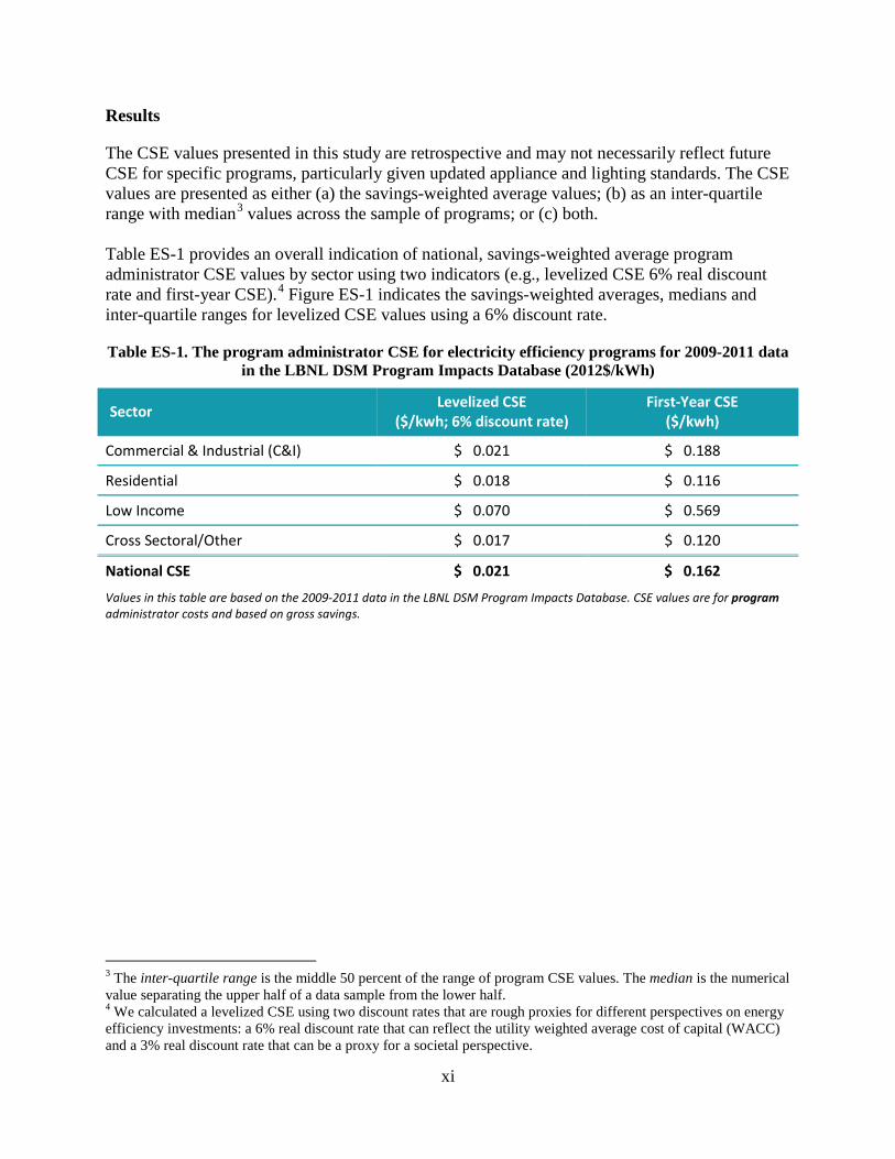
The CSE values presented in this study are retrospective and may not necessarily reflect future CSE for specific programs, particularly given updated appliance and lighting standards. The CSE values are presented as either (a) the savings-weighted average values; (b) as an inter-quartile range with median3 values across the sample of programs; or (c) both. Table ES-1 provides an overall indication of national, savings-weighted average program administrator CSE values by sector using two indicators (e.g., levelized CSE 6% real discount rate and first-year CSE).4 Figure ES-1 indicates the savings-weighted averages, medians and inter-quartile ranges for levelized CSE values using a 6% discount rate.

Table ES-1. The program administrator CSE for electricity efficiency programs for 2009-2011 data in the LBNL DSM Program Impacts Database (2012$/kWh)

Sector Levelized CSE ($/kwh; 6% discount rate)

First-Year CSE ($/kwh)

Commercial & Industrial (C&I) $ 0.021 $ 0.188

Residential $ 0.018 $ 0.116

Low Income $ 0.070 $ 0.569

Cross Sectoral/Other $ 0.017 $ 0.120

National CSE $ 0.021 $ 0.162

Values in this table are based on the 2009-2011 data in the LBNL DSM Program Impacts Database. CSE values are for program administrator costs and based on gross savings.

3 The inter-quartile range is the middle 50 percent of the range of program CSE values. The median is the numerical value separating the upper half of a data sample from the lower half. 4 We calculated a levelized CSE using two discount rates that are rough proxies for different perspectives on energy efficiency investments: a 6% real discount rate that can reflect the utility weighted average cost of capital (WACC) and a 3% real discount rate that can be a proxy for a societal perspective.

xi

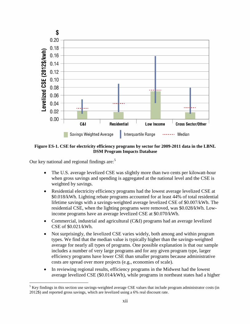
Figure ES-1. CSE for electricity efficiency programs by sector for 2009-2011 data in the LBNL DSM Program Impacts Database

Our key national and regional findings are:5

• The U.S. average levelized CSE was slightly more than two cents per kilowatt-hour when gross savings and spending is aggregated at the national level and the CSE is weighted by savings.

• Residential electricity efficiency programs had the lowest average levelized CSE at $0.018/kWh. Lighting rebate programs accounted for at least 44% of total residential lifetime savings with a savings-weighted average levelized CSE of $0.007/kWh. The residential CSE, when the lighting programs were removed, was $0.028/kWh. Low-income programs have an average levelized CSE at $0.070/kWh.

• Commercial, industrial and agricultural (C&I) programs had an average levelized CSE of $0.021/kWh.

• Not surprisingly, the levelized CSE varies widely, both among and within program types. We find that the median value is typically higher than the savings-weighted average for nearly all types of programs. One possible explanation is that our sample includes a number of very large programs and for any given program type, larger efficiency programs have lower CSE than smaller programs because administrative costs are spread over more projects (e.g., economies of scale).

• In reviewing regional results, efficiency programs in the Midwest had the lowest average levelized CSE ($0.014/kWh), while programs in northeast states had a higher

5 Key findings in this section use savings-weighted average CSE values that include program administrator costs (in 2012$) and reported gross savings, which are levelized using a 6% real discount rate.

xii

average CSE value ($0.033/kWh). Programs in western states are at $0.023/kWh and for the southern states included in the database, the comparable program CSE was $0.028/kWh.

• Natural gas efficiency programs had a national, program administrator savings-weighted average CSE of $0.38 per therm, with significant differences between the C&I and residential sectors (average values of $0.17 vs. $0.56 per therm, respectively).

• The cost of saved energy may vary across program administrator portfolios for reasons that have little to do with programmatic efficiency. In some jurisdictions, a policy mandate of acquiring all reasonably available cost-effective energy efficiency can lead to a focus on more comprehensive programs which will tend to have a higher CSE because they are serving more diverse constituencies and technologies. In other jurisdictions, the focus may be on acquiring the cheapest savings possible.

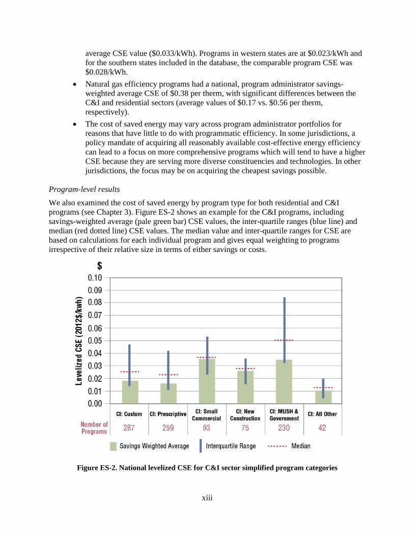
Program-level results We also examined the cost of saved energy by program type for both residential and C&I programs (see Chapter 3). Figure ES-2 shows an example for the C&I programs, including savings-weighted average (pale green bar) CSE values, the inter-quartile ranges (blue line) and median (red dotted line) CSE values. The median value and inter-quartile ranges for CSE are based on calculations for each individual program and gives equal weighting to programs irrespective of their relative size in terms of either savings or costs.

Figure ES-2. National levelized CSE for C&I sector simplified program categories

xiii

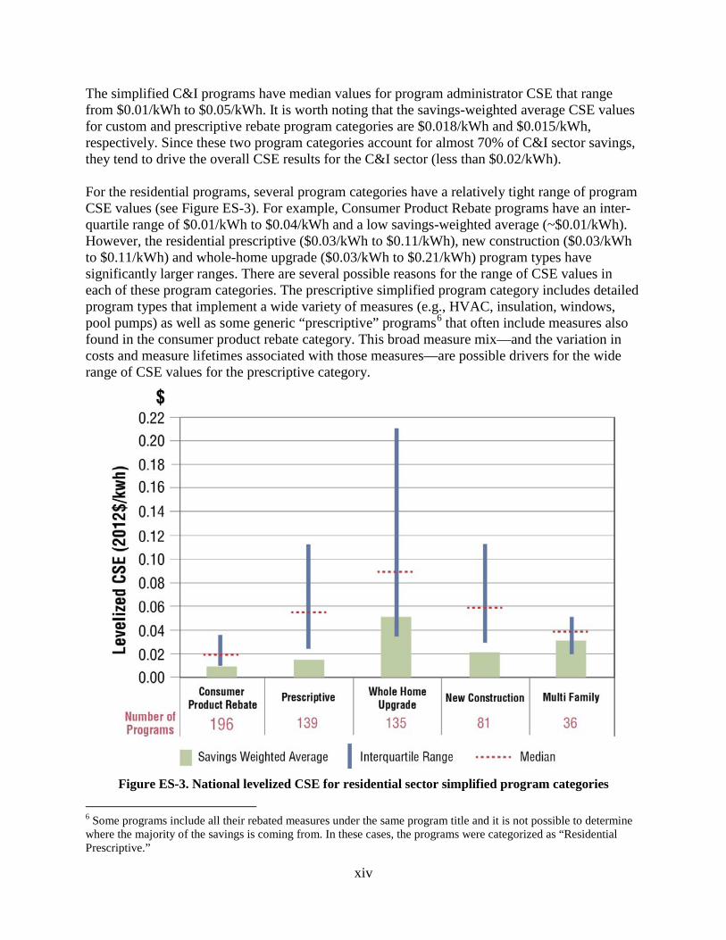
The simplified C&I programs have median values for program administrator CSE that range from $0.01/kWh to $0.05/kWh. It is worth noting that the savings-weighted average CSE values for custom and prescriptive rebate program categories are $0.018/kWh and $0.015/kWh, respectively. Since these two program categories account for almost 70% of C&I sector savings, they tend to drive the overall CSE results for the C&I sector (less than $0.02/kWh). For the residential programs, several program categories have a relatively tight range of program CSE values (see Figure ES-3). For example, Consumer Product Rebate programs have an inter-quartile range of $0.01/kWh to $0.04/kWh and a low savings-weighted average (~$0.01/kWh). However, the residential prescriptive ($0.03/kWh to $0.11/kWh), new construction ($0.03/kWh to $0.11/kWh) and whole-home upgrade ($0.03/kWh to $0.21/kWh) program types have significantly larger ranges. There are several possible reasons for the range of CSE values in each of these program categories. The prescriptive simplified program category includes detailed program types that implement a wide variety of measures (e.g., HVAC, insulation, windows, pool pumps) as well as some generic “prescriptive” programs6 that often include measures also found in the consumer product rebate category. This broad measure mix—and the variation in costs and measure lifetimes associated with those measures—are possible drivers for the wide range of CSE values for the prescriptive category.

Figure ES-3. National levelized CSE for residential sector simplified program categories

6 Some programs include all their rebated measures under the same program title and it is not possible to determine where the majority of the savings is coming from. In these cases, the programs were categorized as “Residential Prescriptive.”

xiv

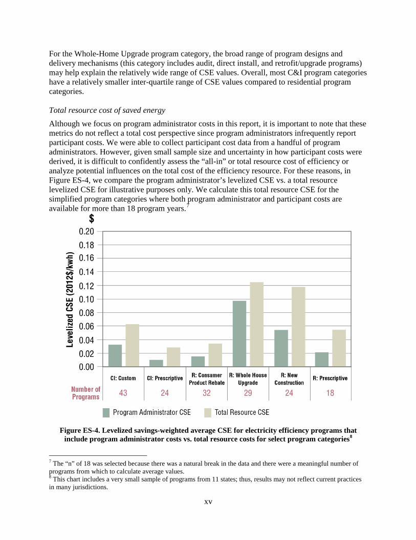
For the Whole-Home Upgrade program category, the broad range of program designs and delivery mechanisms (this category includes audit, direct install, and retrofit/upgrade programs) may help explain the relatively wide range of CSE values. Overall, most C&I program categories have a relatively smaller inter-quartile range of CSE values compared to residential program categories. Total resource cost of saved energy Although we focus on program administrator costs in this report, it is important to note that these metrics do not reflect a total cost perspective since program administrators infrequently report participant costs. We were able to collect participant cost data from a handful of program administrators. However, given small sample size and uncertainty in how participant costs were derived, it is difficult to confidently assess the “all-in” or total resource cost of efficiency or analyze potential influences on the total cost of the efficiency resource. For these reasons, in Figure ES-4, we compare the program administrator’s levelized CSE vs. a total resource levelized CSE for illustrative purposes only. We calculate this total resource CSE for the simplified program categories where both program administrator and participant costs are available for more than 18 program years.7

Figure ES-4. Levelized savings-weighted average CSE for electricity efficiency programs that include program administrator costs vs. total resource costs for select program categories8

7 The “n” of 18 was selected because there was a natural break in the data and there were a meaningful number of programs from which to calculate average values. 8 This chart includes a very small sample of programs from 11 states; thus, results may not reflect current practices in many jurisdictions.

xv

For this small sample of programs, we found that the levelized total resource CSE values are typically double the program administrator CSE with the exception of the Residential Whole Home Upgrade program category (which has a savings-weighted total resource CSE that is about 25-30% higher than the program administrator CSE). Further data collection and analyses could better characterize the way in which the ratio of program administrator costs to participant costs varies as a function of sector, measure types, and market maturity; and how incentives and direct support might be optimized to pay no more than is necessary to meet a state’s efficiency policy objectives. Observations and Recommendations on Reporting

In calculating the CSE, we utilized information on program administrator costs, annual energy savings, estimated lifetime of measures installed in a program, and an assumed discount rate. However, with respect to current program reporting practices, we observed several challenges to the collection of this data for the purposes of calculating the CSE:

• Inconsistencies in the quality and quantity of the costs and savings data led LBNL to develop and attempt to apply consistent data definitions in reviewing and entering program data: o Program administrators in different states did not define savings metrics (e.g.,

varying definitions of net savings) and program costs consistently; and o Market sectors and program types were not characterized in a consistent fashion

among program administrators. • Many program administrators did not provide the basic data needed to calculate CSE

values at the program level (i.e., program administrator costs, lifetime savings, or program-average measure lifetimes), which can introduce uncertainties into the calculation of CSE values (as we developed and utilized methods to impute missing values in some cases).

As a practical matter, the quality and quantity of program data reported by program administrators is an important factor in assessing energy efficiency as a resource in the utility sector. Additional rigor, completeness, standard terms, and consensus on at least essential elements of reporting could pay significant dividends for program administrators and increase confidence in energy efficiency savings among policymakers and other stakeholders—particularly in situations where efficiency is treated as a resource in utility procurement decisions, ISO/RTO forward capacity markets, or as an environmental compliance or mitigation option by state or federal environmental agencies. Of the 45 states currently running utility-customer funded efficiency programs (Barbose et al. 2013), only 31 states provided reporting with sufficient transparency to complete a program-level CSE analysis, and almost all of the 31 states’ data required some interpretation for purposes of regional or national comparison. With more consistent and comprehensive reporting of program results, additional insights can quite possibly be obtained on trends in the costs of energy efficiency as a resource as program administrators scale up efforts, what saving energy costs among an array of strategies, and what and how cost efficiencies might be achieved.

xvi

Therefore, we urge state regulators and program administrators to consider annually reporting certain essential data fields at a portfolio level and more comprehensive reporting of program-level data in order to facilitate the comparison of efficiency program results at state, regional, and national levels. A diagram illustrating this reporting hierarchy approach can be found in Chapter 5, Figure 5-1.

As part of the LBNL CSE Project, we intend to continue collecting energy efficiency program data and analyzing and reporting the CSE for efficiency actions funded by utility customers. We also plan to:

• Work with state, regional, and national stakeholders to encourage the collection ofprogram cost and impact data using a common terminology and program typology asdefined in this report and a companion policy brief (Hoffman et al. 2013). This isimportant for organizing program data into appropriate and consistent categories sothat programmatic energy efficiency, as a regional and national resource, can bereliably assessed.

• Annually compile data reported by program administrators and state agencies fromacross the United States.

• Conduct additional analyses to help increase understanding of factors that influenceEE program impacts, costs and the cost of saved energy.

xvii

1. Introduction

Demand side management (DSM), and end-use energy efficiency specifically, is increasingly being relied upon as a resource for meeting electricity and natural gas system needs within the United States, often because efficiency is quite cost-effective compared to other resource options. For example, 15 states have enacted long-term, binding energy savings targets, often called Energy Efficiency Resource Standards (EERS), and another five states have mandates that program administrators must acquire “all cost-effective energy efficiency.”9 In 2011, U.S. energy efficiency program administrators that manage utility customer-funded efficiency programs spent about $5.4 billion on electric and gas energy efficiency programs (CEE 2013), with spending projected to possibly more than double by 2025 (Barbose et al. 2013).

Electric and natural gas energy efficiency in the United States is pursued through a diverse mix of policies and programmatic efforts, which support and supplement private investments by individuals and businesses. These efforts include federal and state minimum efficiency standards for electric and gas end-use products; state building energy codes; a national efficiency labeling program (ENERGY STAR®); tax credits; and a broad array of largely incentive-based programs for consumers, funded primarily by electric and natural gas utility customers (Dixon et al. 2010) (Barbose et al. 2013).10

These utility customer-funded efficiency programs are overseen by state regulators and administered by more than 100 different entities (e.g., utilities, state energy agencies, non-profit and for-profit third parties) and are the focus of this study. Policymakers, regulators, program administrators and implementers rely on information about lifetime costs and savings of these customer-funded efficiency programs to assess efficiency’s potential, to design and implement programs in a cost-effective manner or to improve program cost effectiveness. Given the expected growth in efficiency funding and the importance of understanding the cost of saved energy (CSE), we initiated this LBNL Cost of Saved Energy Project (CSE Project) to provide a resource for policy makers, regulators and the efficiency industry as a whole.

1.1 Assessing Energy Efficiency as a Resource

The cost and cost effectiveness of utility-customer funded end-use efficiency programs depend on perspective. From the perspective of a participant in a program, their cost is the cost of an efficiency project net of any incentives or support that might be provided by a program administrator. From the program administrator’s perspective, it is the cost of planning, designing, and implementing a program and providing incentives to market allies and end users to take actions that result in energy savings; costs incurred by participants are not considered as part of the program administrator’s costs. The total resource or societal cost perspective takes into

9 States with an EERS as of the date of this report are: AZ, CA, CO, HI, IL, IN, MD, MI, MN, MO, NM, NY, OH, PA, and TX. Six states have a mandate to achieve all cost-effective savings: CA, CT, MA, RI, VT, and WA. 10 For additional energy efficiency market background, please see: The Future of Utility Customer-Funded Energy Efficiency Programs in the United States: Projected Spending and Savings to 2025. http://emp.lbl.gov/publications/future-utility-customer-funded-energy-efficiency-programs-united-states-projected-spend

1

account the costs paid by both the program administrator and the participant to implement the efficiency action. Numerous researchers have estimated the CSE for efficiency programs funded by utility customers (see Appendix A for a description of past and current efforts). These researchers have typically focused on the program administrator perspective (i.e., the program administrator CSE), for two primary reasons. First, in some cases, participant costs are often not collected or reported by program administrators in annual reports (see Chapter 2). Second, when comparing efficiency with supply side resources, some consider that the proper metric is the money paid to obtain the resource by the program administrator as supply-side resources do not consider, or have, participant costs. For this report, primarily because of the first reason, we present program administrator CSE data and analyses. Another consideration for assessing efficiency as a resource is whether CSE values are based on net or gross savings. Net savings are those attributed to a program (for both program participants and non-participants). Gross savings are those associated with the program participants’ efficiency actions, irrespective of the cause of those actions. There is debate about the proper use of net and gross savings in CSE calculations (SEE Action 2012); however, since there is neither sufficient nor consistent data available on net savings, we present CSE values based on gross savings in this study. 1.2 Objectives and Scope

This CSE Project presents and analyzes the costs of acquiring energy savings for different efficiency program types and in different market sectors across the United States. Our objectives are to provide insight into the costs associated with saving a unit of energy and the potential factors that influence those costs. To this end, we hope our work will:

• Benefit policy makers, system planners and other stakeholders by providing continually improving CSE indicators that enable projections of future spending and savings.

• Enable more cost-effective efficiency programs by: o Benchmarking and comparing program implementation approaches across

different markets (e.g., industrial, commercial, small commercial), delivery mechanisms (e.g., direct install versus do it yourself), and design approaches (e.g., prescriptive versus custom rebates);

o Analyzing contextual factors that affect CSE, such as types of programs, measures, program administrator experience, changes in building energy codes and standards, labor costs, climate, state-level policies, and the scale of efficiency investments.

This study is the first technical report of the LBNL CSE Project and provides an overview of project scope, approach and initial findings, including:

• Providing a proof of concept that the program-level cost and savings data can be collected, organized and analyzed in a systematic fashion;

2

• Presenting initial program, sector and portfolio level results for the cost of saved energy for a recent time period (2009-2011); and

• Encouraging state and regional entities to establish common reporting definitions and formats that would make the collection and comparison of CSE data more reliable.

Specifically, this report includes and discusses elements of our approach, including the following:

• Developing the data collection, documentation, and analyses procedures LBNL used to calculate the CSE (Chapter 2);

• Defining program categories as well as cost and savings definitions that allow for consistent, standardized entry of program administrator data into a CSE database (Chapter 2);

• Developing a database of program-level data on energy efficiency program impacts and costs from states with significant utility customer-funded energy efficiency programs (Chapter 2);

• Presenting the range of regional-, state-, sector-, and portfolio-level energy-efficiency program administrator CSE and program-level CSE for a defined set of over 60 program categories (Chapter 3);

• Exploring potential relationships between the program administrator costs of saved energy for specific types of programs and climate zones and adopted building energy codes (Chapter 3);

• Conduct a preliminary statistical analysis that explores factors that may be associated with and influence the cost of saved energy at the portfolio or program level and set the stage for future analyses that will assess additional hypotheses and a broader, more refined range of factors (Chapter 4); and

• Present recommendations for future data collection and analyses (Chapter 5). 1.3 Report Organization

The remainder of this report is organized as follows. Chapter 2 provides an overview of approach used to collect data in the LBNL DSM Program Impacts Database and the challenges associated with collecting, organizing and analyzing the data in a consistent fashion. In Chapter 3, we present descriptive statistics on efficiency program costs and savings followed by presentation of CSE statistics at a national, sector, regional, and state level and for certain program types and in relation to climate zones and building code status. In Chapter 4, we discuss our efforts to define and statistically test some factors that may influence the CSE. Chapter 5 presents a discussion of the key findings and recommendations for regulators and program administrators to consider with respect to CSE-related data collection and reporting. The appendices contain documentation on topics covered in the chapters, including tables of CSE metrics by region, sectors, and program types in Appendix E.

3

2. Approach

The state-by-state evolution of utility customer-funded energy efficiency programs has fostered diversity in these programs’ oversight, design, administration and evaluation. Thus, not surprisingly, information provided to state regulators by program administrators on the impacts and costs of efficiency programs is diverse with respect to the level of specificity and detail required as well as terms and definitions used to describe the costs and impacts of individual programs. In this chapter, we summarize our assembled program data, discuss our approach to compiling, organizing and analyzing the data in a manner that addresses the diversity in reporting practices yet allows for consistent reporting on the cost of saved energy across the country and on the basis of region, market sector, and type of program. This approach included developing an energy efficiency program typology and adopting standard definitions for program characteristics, cost and savings data. We also discuss several major challenges associated with collecting and analyzing program cost and impact data and calculating CSE values given data quality issues. 2.1 Data Summary

The data for this study were drawn from annual reports, mostly for the years 2009–2011, which were prepared by program administrators of efficiency programs funded by the customers of U.S. investor-owned utilities in 31 states. Our energy efficiency program data set comprises expenditure, energy savings and program participation data (where available) reported by 107 program administrators, for a total of 4,184 program records (see Table 2-1). We relied primarily on annual DSM or efficiency reports filed by program administrators with state regulatory agencies because they both typically include data for a portfolio of programs and are publicly available from state regulatory commission filings.11 In some cases, when data were not found or were ambiguous in annual reports, we consulted other reports (e.g., other performance metrics reports filed by investor-owned utilities in California) or solicited additional information directly from the program administrator or regulatory staff. Where required data were not provided in a program administrator’s filed annual report, but provided in third-party program evaluation reports that were included as attachments to the program administrator annual reports, we used data from both to populate what we are calling the LBNL DSM Program Impacts Database (database).12,13

11 The states included in this analysis were selected based on the availability and transparency of program cost and savings data at the individual program level as identified by LBNL researchers in a recent review of customer-funded energy-efficiency programs (Barbose et al. 2013). To the extent that reports were accessible, we collected data for all investor-owned utilities (IOUs) in the target states. Many program administrators had not yet released 2012 program year results during the data collection period for this study; thus our analysis focuses on the 2009-2011 period. We did not include program data from publicly-owned electric utilities and rural electric cooperatives because these utilities often do not report program level data that is publicly available. Future efforts may include data collected from public utilities. 12 We did not rely on individual impact evaluation studies of efficiency programs because the data of interest to this project are usually reported in relatively easily accessible summary form and per program in the annual reports filed with regulators. Moreover, evaluations of individual programs are not always publicly available nor do they always include program or portfolio-related costs. 13 Appendix C describes data that was collected for this research effort, the database configuration, and the data quality assurance/quality control process and procedures.

4

Table 2-1. Summary of energy efficiency program data in LBNL DSM Program Impacts Database14

State First Year of Data

Last Year of Data

Total # of Years

Number of Program

Administrators*

Number of Program Records

AZ 2010 2011 2 3 65

CA 2010 2012 3 4 1210

CO 2009 2011 3 1 110

CT 2009 2011 3 4 60

FL 2011 2011 1 5 88

HI 2009 2011 3 1 21

IA 2009 2011 3 3 171

ID 2010 2011 2 1 40

IL 2008 2011 4 2 85

IN 2009 2012 4 5 244

MA 2009 2011 3 11 403

MD 2010 2011 2 4 126

ME 2009 2011 3 2 22

MI 2009 2011 3 2 81

MN 2009 2011 3 2 141

MT 2011 2011 1 1 19

NC 2009 2011 3 2 37

NH 2009 2011 3 4 90

NJ 2009 2011 3 1 40

NM 2010 2011 2 4 101

NV 2009 2011 3 3 209

NY 2009 2011 3 11 111

OH 2009 2011 3 7 170

OR 2009 2011 3 2 16

PA 2009 2010 2 6 143

RI 2010 2011 2 2 36

TX 2010 2011 2 10 202

14 “Number of Program Records” includes programs that produced energy savings (e.g., residential or commercial rebate programs), programs for which the program administrator did not claim savings (e.g., education and outreach programs or pilot programs), and, in some cases, sector- or portfolio-wide activities (e.g., marketing or internal program evaluation activities).

5

State First Year of Data

Last Year of Data

Total # of Years

Number of Program

Administrators*

Number of Program Records

UT 2009 2011 3 1 41

VT 2009 2011 3 1 18

WA 2010 2011 2 1 42

WI 2009 2011 3 1 42

Totals 107 4184

* In some cases, program administrators who run both gas and electric programs are counted twice for the purposes of separating the reported effects of each program.

Figure 2-1. LBNL DSM Program Impacts Database coverage as compared to national efficiency

spending reported by Consortium for Energy Efficiency (CEE)15

15 CEE Annual Industry Reports can be found here: http://www.cee1.org/annual-industry-reports

6

The efficiency program data that were compiled by LBNL staff into the database represent a significant share of all efficiency programs funded by utility customers in the United States. The database contains programs with total program administrator expenditures of about $7.6 billion (see light and dark blue shading in Figure 2-1). Programs in the LBNL database represent about 25% ($1.1 billion) of 2009 national program expenditures by gas and electric utilities and about 50% of program expenditures in 2010 and 2011 ($2.9B in 2010 and $3.2B in 2011), compared to national efficiency spending as reported by the Consortium for Energy Efficiency (CEE) (see Figure 2-1).16 2.2 Program Typology and Standardized Definitions

We developed program categories in order to characterize and analyze similar types of efficiency program types, as defined by market sector and technology, action, delivery approach, or other common themes. Examples of program categories include commercial prescriptive HVAC programs, low-income programs, and residential whole home direct-install programs. Some program categories are relatively well defined and include a narrow set of technologies (e.g., high-efficiency windows or pool pumps), while other categories are cross-cutting, may span a wide variety of activities (e.g., statewide marketing, take-home energy efficiency kits), and/or target several market sectors (e.g., in-school education programs, lighting technology market transformation programs). The typology grouped and classified energy efficiency programs into three tiers: (1) sector; (2) simplified program categories; and (3) detailed program categories. Figure 2-2 provides a partial snapshot of this three-tiered program typology approach: seven sectors (including one for demand response programs, which are not addressed in this report), 31 simplified efficiency program categories (27 for efficiency programs) and 66 detailed categories (62 for efficiency).17 LBNL has prepared a policy brief that describes the typology in more detail as well as the standardized definitions (Hoffman et al 2013). Appendix B also includes the complete typology and set of definitions. We determined that a three-tiered hierarchy was appropriate because it allowed for flexibility in grouping programs for comparison (e.g., single-measure versus comprehensive whole-building programs or by technology such as lighting vs. HVAC programs) and provides options for different levels of analysis. Moreover, in some cases, the detailed program category tier narrowed the range of installed measures for a program type, thus reducing the uncertainty in derivation of measure savings and lifetime savings across measures installed in that program. For example, we defined three detailed program categories that fall under the simplified program

16 However, as noted below and in Chapter 3, some of the data were not utilized for the data presentations, CSE metrics and analyses due to missing data. For example, the programs indicated as Combined Fuel in this figure were not included in the cost of saved energy analyses, because the costs borne by electricity and gas utility customers could not be determined for this subset of programs. Without the useable data, the database still contains about 45-50% of the national spending estimate. 17 The relatively large number of simplified and detailed categories was necessary to capture the wide range of common program offerings throughout the country. We also included some program types in the detailed typology because they have regional significance (e.g., pool pump programs in the Southwest, data center programs in New York, Washington and California), or the program types appear to be emergent (e.g., financing programs, residential behavior-based efficiency programs).

7

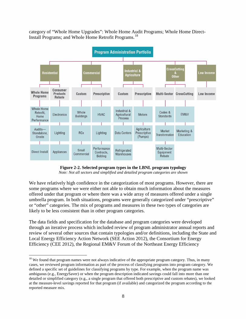
category of “Whole Home Upgrades”: Whole Home Audit Programs; Whole Home Direct-Install Programs; and Whole Home Retrofit Programs.18

Figure 2-2. Selected program types in the LBNL program typology

Note: Not all sectors and simplified and detailed program categories are shown

We have relatively high confidence in the categorization of most programs. However, there are some programs where we were either not able to obtain much information about the measures offered under that program or where there was a wide array of measures offered under a single umbrella program. In both situations, programs were generally categorized under “prescriptive” or “other” categories. The mix of programs and measures in these two types of categories are likely to be less consistent than in other program categories. The data fields and specification for the database and program categories were developed through an iterative process which included review of program administrator annual reports and review of several other sources that contain typologies and/or definitions, including the State and Local Energy Efficiency Action Network (SEE Action 2012), the Consortium for Energy Efficiency (CEE 2012), the Regional EM&V Forum of the Northeast Energy Efficiency

18 We found that program names were not always indicative of the appropriate program category. Thus, in many cases, we reviewed program information as part of the process of classifying programs into program category. We defined a specific set of guidelines for classifying programs by type. For example, when the program name was ambiguous (e.g., EnergySaver) or when the program description indicated savings could fall into more than one detailed or simplified category (e.g., a single program that offered both prescriptive and custom rebates), we looked at the measure-level savings reported for that program (if available) and categorized the program according to the reported measure mix.

8

Partnerships (NEEP 2011), and the NEEP Regional Energy Efficiency Database (REED 2013). We shared a draft of our categories and definitions and had several discussions with representatives from CEE, NEEP and the American Council for an Energy-Efficient Economy (ACEEE); and made revisions based on their input. For the demand-response program categories, we relied on program categories defined by the Federal Energy Regulatory Commission (FERC) for its national surveys (FERC 2012), although demand-response program data are not included in this study. We also defined program cost and energy savings (impacts) data fields as part of our effort to classify and report program information in a consistent fashion across program administrators and states.19

• Program Administrator Costs: The primary cost data used in this report are the program administrator costs which include: (1) program administration planning and delivery; (2) engineering or technical support; (3) services provided by implementation contractors; (4) marketing, education and outreach; (5) direct rebates or financial incentives to program participants; and (6) evaluation, measurement and verification costs (see Table 2-1).20 Program administrator costs exclude participant costs and performance incentives for program administrators (e.g., utility shareholder incentives).21 For each program we collected from one to four years of data.22 We made inflation adjustments to the program cost data provided by program administrators so that all cost data are reported in 2012$.23 We chose to use 2012 as our base year because 2012 is the most recent year for which an annual implicit price deflator for GDP is available from the U.S. Bureau of Economic Analysis. We would have preferred to also report CSE values based on participant, as well as program administrator, costs; however, we found that few program administrators reported participant costs in their annual reports (see Appendix C).

• Program Savings: The State and Local Energy Efficiency Action Network’s Energy Efficiency Program Impact Evaluation Guide (SEE Action 2012) was the primary source used to describe and define the program energy savings indicators in a consistent fashion.24 The SEE Action Guide was particularly important for providing

19 Program cost and savings definitions tend to be consistent within a state, even if there are multiple program administrators. 20 Some program administrators did not include program-level costs for activities such as marketing/outreach, education, and evaluation, but instead accounted for those expenditures at the sector or portfolio level. 21 We did not report program administrator performance incentives because actual awards of performance incentives are not often included in annual reports filed by program administrators, and are frequently awarded at a significantly later date. 22 Some program administrators included prior years’ data in their reports in addition to the 2009–2011 period. 23 Costs can be presented in nominal (or current) or real (or constant) dollar terms. Nominal values are economic units measured in terms of purchasing power of the date in question. Real dollar values are economic units measured in terms of constant purchasing power. A real value is not affected by general price inflation and can be estimated by deflating nominal values with a general price index, such as the implicit deflator for gross domestic product or the Consumer Price Index. From OMB Circular A-94 Guidelines And Discount Rates For Benefit-Cost Analysis of Federal Programs. We used the GDP implicit price deflator published regularly by the U.S. Bureau of Economic Analysis. 24 The SEE Action Guide describes common terminology, structures, and approaches used for determining savings from energy efficiency programs guide. The definitions in the SEE Action Guide incorporated input from program

9

data definitions for net and gross energy savings and lifetime energy savings, which for this report are assumed to take place at the end-use site where the efficiency actions were implemented.

Table 2-2 provides abridged definitions for key program data in the Database (see Appendix B for the complete glossary of energy efficiency program data fields).

Table 2-2. Abridged definitions for selected program cost and savings data

Term Definition

Program Administrator Costs

Program administrator costs include the costs of designing programs and portfolios; directing, managing and paying implementation contractors; marketing, education and outreach (ME&O); program and portfolio evaluations; and incentives to both program participants (or end users) and to both mid-stream and upstream allies in the market (e.g., financing and services such as installations or free audits).

Program Average Measure Lifetime

Weighted average economic lifetime (years) of all measures installed in a program year in a specified program.

Annual Gross Savings Gross annual incremental savings (kWh or therm) as reported by the program administrator using their own staff or evaluation firm, after the subject energy efficiency activities have been completed. Gross savings are the change in energy consumption resulting from program-related actions taken by program participants regardless of why they participated. Note that these are annualized “full-year” savings, regardless of when measures were installed during the program year. Per the SEE Action reference (SEE Action 2012) these may be Claimed or Evaluated Savings.

Lifetime Gross Savings The expected gross savings (GWh or therm) over the lifetime of the measures installed under the subject program. For our analysis, where available, we relied on lifetime savings reported by the program administrator.

The detailed program categories and data definitions described in this section have been adapted by CEE for its own 2013 annual surveys of the efficiency program industry.25 We hope that other entities will consider using them as well and to support that objective, as part of the CSE Project, LBNL plans to gather feedback from stakeholders via an annual or biennial process to modify, add or subtract program categories as program offerings change or to address potentially needed clarifications in the definitions and categories.

administrators, state regulators, and other stakeholders from a number of states and regions and included a review and synthesis of definitions used in a broad set of energy efficiency glossaries. 25 As part of its 2013 annual “State of the Industry” survey, CEE is collecting program-level energy efficiency and demand response program data from program administrators using the LBNL program categories described in this report as well as the definitions from the SEE Action guide.

10

2.3 Challenges in Consistent and Standardized Reporting of Program Data

When data are compiled from multiple states and program administrators, terminology differences can potentially make it difficult to conduct comparative analysis across states or program administrators. This was a primary rationale underlying our effort to develop a program typology and standardized definitions so that we could conduct a comparative analysis of energy efficiency program impacts and costs. However, even with the typology and definitions, there are two key data challenges. First, we assume that all expenditure, savings and participation data reported by a program administrator are accurate. Given our time and resources, this is a reasonable starting assumption; however, it should be noted that the range of effort placed into documenting impacts by program administrators varies significantly among states (SEE Action 2012). Second, in reviewing information on efficiency programs funded by U.S. utility customers, we found that program data are often not defined and reported consistently among states. Specifically, we identified three key concerns in compiling and analyzing program information on a regional or national basis, some of which are addressed by the common typology and standardized definitions:

1. Energy savings and program costs are not defined consistently. The most common

discrepancies can be found in the definitions of net energy savings. Examples of other program data where differences are found across states include:

• The term “annual energy savings” typically is understood as shorthand for annualized incremental energy savings, but some entities—including resource planners—apply a different meaning that includes savings resulting from prior years’ activities.

• The definition of measure lifetime, how a program’s average measure lifetime is determined, and the estimated measure lifetime values for the same measures or program types varies among states.

• Some program administrators report end-use site savings and others report savings at the power plant bus bar (for electricity efficiency programs).

• Most program administrators do not count their own performance incentives among program costs, although some do. The definitions of other cost categories (e.g., marketing costs, general consumer education, and evaluation) also vary among states.

2. Program data are not reported consistently across states. For example, some states report just gross or net energy savings; others report both. Similarly, many efficiency annual reports only include first-year savings and not lifetime savings.26 With respect to cost data, program administrators often classify costs differently among administration, marketing and outreach, incentives and participant costs. Some program administrators

26 We found that only about a quarter of the program reports that were reviewed included information on measure lifetimes or lifetime savings, although this information is required to assess program cost effectiveness. See below, in the section on adjustments for missing data, for discussion of how measure lifetime variation creates uncertainty in the calculation of CSE.

11

also report certain costs (e.g., marketing, evaluation) at the portfolio or sector level, while others account for those costs at the program level.

3. Programs and sectors are not characterized in a standardized fashion. Programs targeting specific building types or consumers can be included under different sectors from state to state (e.g., multi-family residential structures are sometimes categorized as commercial programs). Moreover, the types of activities and measures that are included under the same program title (e.g., custom vs. combination custom/prescriptive programs) also vary.

We suggest that readers consider these above issues when utilizing the information in this report for their own uses and understanding of the cost of saved energy. 2.4 Calculating and Using the Cost of Saved Energy

The program administrator’s CSE is a useful metric for comparing the relative costs of efficiency programs and for comparing an energy efficiency option to other demand and supply choices for serving electricity and natural gas needs27. However, the cost of saved energy is not a test of cost effectiveness (e.g., one of the screening tests used by program administrators) because: (1) it does not capture the full benefits to utility customers and shareholders (e.g., avoided generation capacity, avoided transmission and distribution investments, avoided environmental compliance costs); (2) benefits are not monetized but reflected simply in energy units of kilowatt hours or therms, the cost of which will vary by utility; and (3) energy is saved at the end use, not the power plant.28 In this report, we use gross energy savings (rather than net savings) in the CSE calculations primarily because of data availability and comparability reasons: (1) more administrators reported gross savings than net; and (2) net savings are defined relatively inconsistently, as compared to gross savings, among program administrators and states. We also report savings at the end-user level (and not at the busbar or power plant source), because this is what most program administrators report. It is important to note that savings from electricity efficiency programs reported at the busbar would be higher than at the end-use level because we are accounting for distribution and transmission losses (losses also occur in the natural gas network as well).29

27 According to the Energy Information Administration, “levelized cost is often cited as a convenient summary measure of the overall competiveness of different generating technologies. It represents the per-kilowatt hour cost (in real dollars) of building and operating a generating plant over an assumed financial life and duty cycle. Key inputs… include overnight capital costs, fuel costs, fixed and variable operations and maintenance (O&M) costs, financing costs, and an assumed utilization rate for each plant type. http://www.eia.gov/forecasts/aeo/electricity_generation.cfm 28 The equation also is inverted, with costs in the numerator and benefits (in energy units) in the denominator—the reverse of the benefit/cost ratios that are a key determinant of cost effectiveness. 29 This is an important consideration if the CSE values were to be compared with costs of electricity generation resources, which typically are indicated as busbar values.

12

We calculate the cost of saved energy (CSE) metrics in three ways: (1) a cost of lifetime saved energy; (2) a levelized cost of energy savings using two discount rates (3% and 6% real); and (3) a cost of first-year energy savings. See Table 2-3 for definitions of these CSE metrics and their common uses.

Table 2-3. Program administrator cost of saved energy metrics: definitions and potential uses

Program Administrator Cost Metric

Shortened Term What is Measured Potential Uses

Cost of Lifetime Energy Savings

Lifetime CSE The cost of acquiring energy savings that accrues over the economic lifetime of the actions taken through a program/sector/portfolio. Calculated by dividing program administrators’ costs by the gross savings.

• Used by program administrators for designing programs and portfolios, e.g., for depth of savings and cost effectiveness

• Used by planners and other stakeholders to project efficiency as a resource, develop load forecasts, etc.

Levelized Cost of Energy Savings

Levelized CSE The cost of acquiring energy savings that accrue over the economic lifetime of the actions taken through a program/sector/portfolio, amortized over that lifetime and discounted back to the year in which the costs are paid and the actions are taken

• Same uses as lifetime savings

• Useful to program administrators, regulators and other stakeholders who want to compare particular demand-side options with other demand, and supply-side, resources

Cost of First-Year Energy Savings

First-Year CSE The cost of acquiring a single year of annualized incremental energy savings through actions taken through a program/sector/portfolio. Calculated by dividing the program administrators’ costs by the first year incremental savings.

• Useful for program administrators in program design

The cost of saved energy can be useful to various stakeholders. For example, state regulators can use both first-year and lifetime CSE values as quick metrics for assessing whether a program or portfolio looks like a reasonable expenditure of utility customer funds. A program administrator that is considering offering a comprehensive residential energy upgrade program may want to compare that program’s estimated per-unit cost performance against average costs and the range of costs for similar programs. Based on the comparison, the program administrator may want to

13

look at the design of comparable programs for potential cost efficiencies. Regulators and resource planners can use the levelized CSE in the initial screening analysis of various supply- and demand-side resources. Resource planners also can use the lifetime CSE to convert approved budgets for demand-side management plans into energy savings estimates that then can be used in scenario or sensitivity analysis of future load forecasts. Finally, based on the limited participant cost data reported by program administrators, we calculate a total resource CSE for illustrative purposes in Chapter 3. This calculation presents the net total costs, including both program and participant costs, for the efficiency resource. A levelized total resource CSE might also be useful to program administrators, regulators and other stakeholders who want to compare particular demand-side options with other demand and supply-side resources. 2.4.1 Levelized Cost of Saved Energy

The lifetime cost of energy savings metric is a simple, straight-forward calculation although it ignores changes in the value of money between an initial investment and future energy savings. Meier (1982) included the time value of money (discount rate) to calculate the “cost of conserved energy” (CCE) or what we are calling the “levelized cost of saved energy”. Meier found that inclusion of the discount rate raises the CCE because of discounting future benefits, yet provides a basis for comparing the CCE for measures that have different lifetimes and can be compared to retail rates and levelized costs of supply-side resources.30 A similar accounting framework, the levelized cost of energy (LCOE), often is applied to assessing the economic competitiveness of diverse generation sources (U.S. Energy Information Administration 2013). We calculated a levelized CSE using two discount rates31 that are rough proxies for different perspectives on energy efficiency investments: a 6% real discount rate that can reflect the utility weighted average cost of capital (WACC) at present and a 3% real discount rate that can be a proxy for a societal perspective. The levelized CSE calculation is as follows:

𝐿𝑒𝑣𝑒𝑙𝑖𝑧𝑒𝑑 𝐶𝑆𝐸 (𝑖𝑛 $/𝑢𝑛𝑖𝑡 𝑒𝑛𝑒𝑟𝑔𝑦, 𝑒.𝑔. , 𝑘𝑊ℎ, 𝑡ℎ𝑒𝑟𝑚,𝐵𝑡𝑢) = (𝐶 𝑥 (𝐶𝑎𝑝𝑖𝑡𝑎𝑙 𝑅𝑒𝑐𝑜𝑣𝑒𝑟𝑦 𝐹𝑎𝑐𝑡𝑜𝑟))/(𝐷)

𝐶𝑎𝑝𝑖𝑡𝑎𝑙 𝑅𝑒𝑐𝑜𝑣𝑒𝑟𝑦 𝐹𝑎𝑐𝑡𝑜𝑟 = [𝐴 ∗ (1 + 𝐴)^𝐵]/[(1 + 𝐴)^𝐵 − 1] Where:

A = Discount rate

30 See Appendix A for further discussion of the history of efficiency CSE analyses 31 Discount Rate: An interest rate applied to a stream of future costs and/or monetized benefits to convert those values to a common period, typically the current or near-term year, to measure and reflect the time value of money. It is used in benefit-cost analysis to determine the economic merits of proceeding with a proposed project, and in cost-effectiveness analysis to compare the value of projects. The discount rate for any analysis is either a nominal or a real discount rate. A nominal discount rate is used in analytic situations when the values are in then-current or nominal dollars (reflecting anticipated inflation rates). A real discount rate is used when the future values are in constant dollars and can be approximated by subtracting expected inflation from a nominal discount rate (SEE Action Network 2012).

14

B = Estimated program measure life in years

C = Total program cost in 2012$

D =Annual kWh saved that year by the energy efficiency program

This formula is the classic definition of a compound interest calculation used to calculate equivalent annual net disbursements.

The discount rate can have a significant impact on the calculated CSE. For example, for a program with an average measure lifetime of 20 years, a discount rate of 6% will indicate a levelized CSE that is about 30% higher than the same program if a discount rate of 3% were used. See Appendix D for further discussion of the factors considered in choosing these two illustrative interest rates. 2.5 Treatment and Adjustments for Missing Data

In calculating CSE for efficiency programs, we encountered several data completeness issues that needed to be resolved:

• Many programs’ data included neither program measure lifetime nor gross lifetime savings. This information is necessary to calculate lifetime and levelized CSE;

• Some combined gas and electric program administrators reported separate savings for their electric and gas programs but did not separate their electric and gas program costs; and,

• Most program administrators reported end-use energy efficiency savings while others reported savings at the source of the electricity (generation or busbar savings). Natural gas savings are usually considered the same at the end-use site and at points along the gas distribution, although there is the potential for per unit losses from the natural gas source to the end user.

In addition, for the few program administrators that reported only net savings, we calculated gross savings by dividing reported net savings by a net-to-gross ratio32 when this ratio was provided in related references for the subject programs.33 Furthermore, some program reports provided no cost data and others provided no savings data; these programs were excluded from the CSE analysis. These adjustments resulted in program data from 100 program administrators in the database being utilized in calculating CSE values in this study.34

32 The net-to-gross ratio is the net program impact (energy savings) divided by the gross program impact. 33 In Massachusetts and New York, program administrators reported net savings and did not provide net-to-gross ratios in their annual efficiency reports. In these cases, we applied net-to-gross ratios reported in the 2011 REED database and applied the program level ratios to the previous two years included in this analysis (2009-2010). New Hampshire program administrators reported net lifetime savings for 2009-2010. We were not able to generate a gross lifetime or annual incremental savings values needed to calculate the CSE and therefore those years were dropped from the analysis. 34 Data from 100 of the 107 program administrators whose data are in the LBNL DSM Program Impacts Database are included in this Chapter. The seven program administrators that were excluded represent about eight percent of the total costs for programs in the Database. Three program administrators are excluded because their combined gas and electric program costs could not be separated out by fuel type, three program administrators were excluded because they did not report expenditures at the program level, and one program administrator was excluded because it reported net savings in a manner that did not allow determination of gross savings. Two years of program data

15

2.5.1 Program Average Measure Lifetime

The CSE calculation takes into account the costs incurred to implement the measures, which in the database all occur during the program year,35 and the savings that occur over the lifetime of the implemented measures. However, program administrators reported lifetime savings for only about 44% of the programs years in the collected annual reports (see Appendix C).36 Another way to calculate the lifetime savings is to multiply the first-year savings by the program average measure lifetime (program lifetime)37, which we interpret as the lifetimes of the various measures installed through a program weighted by their respective savings. However, even fewer program administrators reported any form of a program lifetime—about 26% of electric and 30% of gas programs for the 2009–2011 period (see Appendix C). For the programs that did report a lifetime value, program average measure lifetimes varied widely within many of the detailed program categories.38 For example, the median program lifetime for residential new construction programs is 18 years, with a program life of 14 and 25 years at the 25th and 75th percentile for programs in the database. Figure 2-3 shows the range, inter-quartile range, and median program lifetime values reported for a selected sample of detailed program categories. Given the limited availability of lifetime savings and program lifetime values, we developed the following set of decision rules, or protocol, for defining lifetime savings for each program in the database:

1. When available, use the program lifetime savings reported for the program by the program administrator;

2. When program administrator did not report program lifetime savings, but did report program average lifetime value, we multiplied this value by the reported first-year savings to calculate the program’s lifetime savings;39

from three other program administrators were not used in the CSE analysis because these program administrators reported net savings in a manner that did not allow determination of gross savings; however, the third year of data for those three program administrators was used. 35 Some project installations may be completed after the end of the program year but are accrued to the program year in which the project was initiated (e.g., customer has signed up, equipment installation has been scheduled, equipment installation has begun but not been completed). Some energy efficiency actions also may require ongoing, incremental operations and maintenance expenditures (compared to the baseline equipment), which are not considered in this study, which is consistent with most energy efficiency program assessments. 36 There are more than 4,000 program years in the database, where we count each program in each year of implementation separately. 37 Measure lifetime, also called effective useful life (EUL), is based on the lifetime of equipment installed or measures implemented and measure persistence (as opposed to savings persistence). In many energy efficiency programs, the estimated EUL takes into account both the expected remaining life of the measure being replaced and the expected changes in operational baselines over time (Mass Save 2011, SEE Action 2012). 38 A number of factors may contribute to the variation in reported measure lifetimes including the unique mix of measures implemented for a program (particularly for programs that contain a wide range of longer- and shorter-lived measures) and different assumptions and/or methodologies used to determine measure lifetime used by program administrators. 39 Some program administrators document the average measure lifetime for programs that installed a mix of measures. The most common approach used by program administrators is to weight the program average measure lifetime by respective measure savings. We applied this approach for all of the reported program measure lifetimes.

16

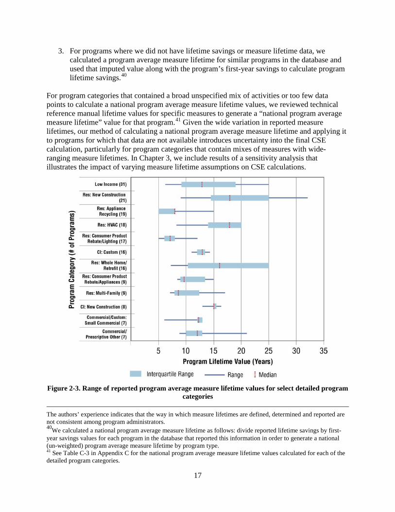
3. For programs where we did not have lifetime savings or measure lifetime data, we calculated a program average measure lifetime for similar programs in the database and used that imputed value along with the program’s first-year savings to calculate program lifetime savings.40

For program categories that contained a broad unspecified mix of activities or too few data points to calculate a national program average measure lifetime values, we reviewed technical reference manual lifetime values for specific measures to generate a “national program average measure lifetime” value for that program.41 Given the wide variation in reported measure lifetimes, our method of calculating a national program average measure lifetime and applying it to programs for which that data are not available introduces uncertainty into the final CSE calculation, particularly for program categories that contain mixes of measures with wide-ranging measure lifetimes. In Chapter 3, we include results of a sensitivity analysis that illustrates the impact of varying measure lifetime assumptions on CSE calculations.

Figure 2-3. Range of reported program average measure lifetime values for select detailed program

categories

The authors’ experience indicates that the way in which measure lifetimes are defined, determined and reported are not consistent among program administrators. 40We calculated a national program average measure lifetime as follows: divide reported lifetime savings by first-year savings values for each program in the database that reported this information in order to generate a national (un-weighted) program average measure lifetime by program type. 41 See Table C-3 in Appendix C for the national program average measure lifetime values calculated for each of the detailed program categories.

17

2.5.2 Cost Data for Combined-Fuel Programs

Some program administrators of combined-fuel programs reported separate electric and gas savings values but did not report separate costs for electric and gas programs or measures. For those program administrators where we could not reliably calculate the per-kWh and per-therm CSE from the reported data, we obtained additional information that enabled us to calculate reasonable estimates of the disaggregated electric and gas expenditures for the following combined fuel utility cases:

• The California combined-fuel utilities did not provide separate electric and gas cost data. However, one of the utilities provided program-level data on the net monetized benefits of the programs, allocated by fuel. We were then able to estimate that utility’s combined electric and gas program costs by fuel (electricity and natural gas) based on the program’s share of savings allocated to each fuel.

• A New England combined-fuel utility that had not reported separate gas and electric cost data later provided estimates of the ratio of gas and electric costs which were applied to that utility’s data.

Other program data from program administrators for which we could not disaggregate electric and gas program costs were included in the overview of program spending and savings presented at the beginning of Chapter 2, but excluded from the dataset used to calculate CSE.42 2.5.3 End-Use versus Source and Busbar Energy Savings

Most state program administrators reported end-use energy efficiency savings; however, there were a few program administrators that reported both end-use and busbar, and a handful that only reported busbar savings. For the purposes of this report, we followed the following decision rules:

• Where program administrators reported both end-use and busbar savings, we used end-use savings;

• Where program administrators are not clear, or do not explicitly state that the savings is end-use, we treat the savings values as end-use savings;

• Where program administrators only reported a busbar savings value, we identified a line loss estimate and calculated that end-use savings.43

42 Wisconsin’s single statewide program administrator was included in the program spending and savings overview but excluded from the CSE results because the program administrator did not provide disaggregated electric and gas program expenditures data. 43 For a discussion on line losses, please see: http://www.raponline.org/ document/download/id/4537

18

3. Results—Utility Customer-Funded Programs: Costs and Savings

In this chapter, we first present a national overview of electric and gas energy end-use efficiency program administrator expenditures and savings, including summaries by market sector and region for the programs in the LBNL DSM Program Impacts Database (database). We then present ranges of program administrator cost of saved energy (CSE) values, mostly for electricity efficiency programs (as they represent about 80% of program expenditures), on a national, regional, and state basis. Some CSE values are presented at the sector and program level as well. We also include sensitivity analyses on the impact of assumed measure lifetimes on the CSE (one of the data issues raised in Chapter 2). Finally, we present CSE results for those programs where program administrators reported program administrator costs and participant costs (what some refer to as the total resource cost). The results presented in this chapter represent a significant portion of the efficiency programs funded by customers of U.S. investor-owned utilities during 2009, 2010, and 2011. However, when using the information, the reader should recognize that they are not necessarily a representative sample, particularly for some regions of the country where annual reporting is not prevalent. 3.1 Energy Efficiency Program Administrator Expenditures and Savings

3.1.1 Electric Programs

Program administrator expenditures for identifiable electricity efficiency programs44 in the database, for the years 2009–2011, totaled just under $5.3 billion (in 2012$) with commercial/industrial programs (C&I) programs representing about 60% of expenditures and residential programs comprising about 30% of the expenditures (see Table 3-1). In terms of how electricity savings vary by sector for the programs in the database, the answer depends on whether first year or lifetime savings are considered (see Figure 3-1). The savings accruing from C&I sector programs accounted for 53% of the aggregate first-year savings and 62% of the aggregate lifetime savings. Residential programs’ share of first-year savings was higher than their share of expenditures; residential programs made up 29% of expenditures but garnered 40% of first-year savings and 31% of lifetime savings. On the other hand, low-income programs represent 6% of the total expenditures and 2% of first-year and lifetime savings.

44 Eighty-eight program administrators reported electric program data.

Attributes of Information Reported in this Chapter

Costs refer to program administrator costs only; the CSE values exclude participant costs unless specifically indicated otherwise.

Savings are based on gross savings reported by the program administrator unless specifically indicated otherwise. For program administrators that only reported net savings values, we calculated gross savings values using net-to-gross ratios. Savings values are also based on savings at the end-use site and not at the power plant or natural gas pumping station and thus do not account for transmission and distribution losses. See Chapter 2 for more detailed explanation.

Lifetime energy savings, when not reported by the program administrator (which was the case for about 50% of the programs), were calculated per the protocol described in Chapter 2.

19

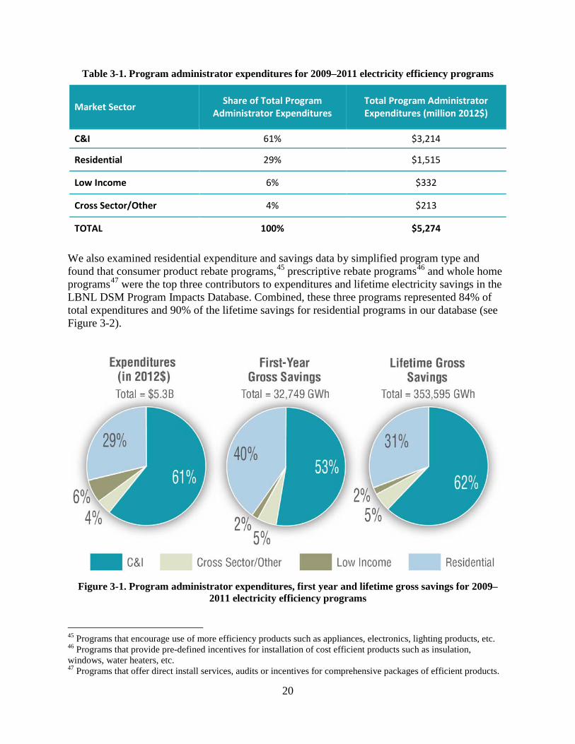
Table 3-1. Program administrator expenditures for 2009–2011 electricity efficiency programs

Market Sector Share of Total Program Administrator Expenditures

Total Program Administrator Expenditures (million 2012$)

C&I 61% $3,214

Residential 29% $1,515

Low Income 6% $332

Cross Sector/Other 4% $213

TOTAL 100% $5,274

We also examined residential expenditure and savings data by simplified program type and found that consumer product rebate programs,45 prescriptive rebate programs46 and whole home programs47 were the top three contributors to expenditures and lifetime electricity savings in the LBNL DSM Program Impacts Database. Combined, these three programs represented 84% of total expenditures and 90% of the lifetime savings for residential programs in our database (see Figure 3-2).

Figure 3-1. Program administrator expenditures, first year and lifetime gross savings for 2009–

2011 electricity efficiency programs

45 Programs that encourage use of more efficiency products such as appliances, electronics, lighting products, etc. 46 Programs that provide pre-defined incentives for installation of cost efficient products such as insulation, windows, water heaters, etc. 47 Programs that offer direct install services, audits or incentives for comprehensive packages of efficient products.

20

Figure 3-2. Program administrator expenditures and lifetime gross savings by simplified program category for 2009–2011 residential electricity efficiency programs

Other observations from the database’s residential electricity program data, as shown in Figure 3-2, are:

• Consumer Product Rebates accounted for about 29% of total residential program expenditures, but over half of the lifetime savings;

• Residential Prescriptive programs accounted for similar percentages of expenditures and lifetime savings, both 26%;

• Whole Home Upgrade programs represented about 29% of aggregated expenditures and12% of the lifetime electricity savings;

• New Construction programs accounted for 5% of residential program expenditures and 6% of the sector’s lifetime savings,

• Multifamily programs accounted for 5% of expenditures and 3% of lifetime savings, and

• Behavior and Education programs make up 3% of expenditures but less than 1% of lifetime savings.

To illustrate the power of a program-level database, we analyzed the four detailed program types that are included in the residential Consumer Product Rebate program category that covers 52% of the residential lifetime electricity savings (see Figure 3-3). This analysis indicated that lighting rebate programs accounted for over 80% of all gross electricity savings attributed to the consumer product rebates in the program administrator program reports we compiled. This means that lighting rebates represent at least 44% of total residential lifetime savings.48 Appliance Recycling programs (which we also included in the product rebate category)

48 We indicate at least 44% because other program types also can, and often do, include lighting related products.

21

accounted for 6% and appliance rebates made up 2% respectively of all residential sector lifetime gross savings. Consumer Electronics programs, the fourth detailed program type in the consumer product rebate category, garnered less than 1% of residential sector savings.

Figure 3-3. Lifetime gross electricity savings for 2009-2011 residential consumer product rebate programs

We also analyzed C&I sector expenditure and savings data by simplified program type (see Figure 3-4) and found the following:

• At 36%, custom programs represented the largest share of all C&I expenditures as well as the largest share of all C&I total lifetime savings at 38%.

• Prescriptive and small commercial programs accounted for comparable shares of C&I expenditures at about 21% each; although reported lifetime savings were much greater for prescriptive programs (30% of all savings) compared to small commercial programs (11% of all C&I savings).

• Commercial new construction programs accounted for 12% of C&I expenditures and 10% of the sector’s savings.

• Programs specifically targeting the institutional market (municipal and state governments, universities, colleges, K-12 schools and hospital/healthcare facilities, also collectively known as the MUSH market) made up 7% of total C&I program expenditures and 4% of the savings, although it should be noted that institutional sector customers can and do participate in many other types of C&I programs as well.

22

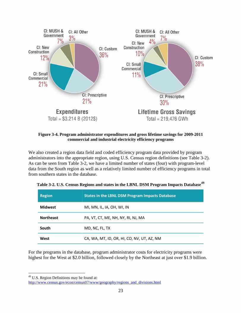
Figure 3-4. Program administrator expenditures and gross lifetime savings for 2009-2011 commercial and industrial electricity efficiency programs

We also created a region data field and coded efficiency program data provided by program administrators into the appropriate region, using U.S. Census region definitions (see Table 3-2). As can be seen from Table 3-2, we have a limited number of states (four) with program-level data from the South region as well as a relatively limited number of efficiency programs in total from southern states in the database.

Table 3-2. U.S. Census Regions and states in the LBNL DSM Program Impacts Database49

Region States in the LBNL DSM Program Impacts Database

Midwest MI, MN, IL, IA, OH, WI, IN

Northeast PA, VT, CT, ME, NH, NY, RI, NJ, MA

South MD, NC, FL, TX

West CA, WA, MT, ID, OR, HI, CO, NV, UT, AZ, NM

For the programs in the database, program administrator costs for electricity programs were highest for the West at $2.0 billion, followed closely by the Northeast at just over $1.9 billion.

49 U.S. Region Definitions may be found at: http://www.census.gov/econ/census07/www/geography/regions_and_divisions.html

23

http://www.census.gov/econ/census07/www/geography/regions_and_divisions.html

Program administrator expenditures totaled just under $1 billion in the Midwest and about $505 million in the South (see Figure 3-5).

Figure 3-5. Program administrator expenditures by region for 2009-2011 electricity efficiency programs

The regional breakdown of lifetime savings for programs in the database looks much different compared to expenditures (see Figure 3-6). Program administrators in the Midwest reported about 20% more lifetime electricity savings than program administrators in the Northeast and about 75% of the savings for program administrators in the West, although expenditures in the Midwest were less than half of those in the West or Northeast. As can be seen from Figure 3-5 and Figure 3-6, savings reported by program administrators come predominantly from the C&I sector, except for the South where residential and C&I program savings are more balanced. In the Midwest, C&I programs accounted for a little more than half of the region’s total expenditures, but C&I programs accounted for nearly 70% of the savings. In the West, the expenditure and savings proportions were more comparable; C&I programs accounted for about 60% of total expenditures and about 65% of the savings, while 27% of expenditures and 21% of savings occurred in the residential sector. Low-income program expenditures were significantly higher in the Northeast than in the other regions.

24

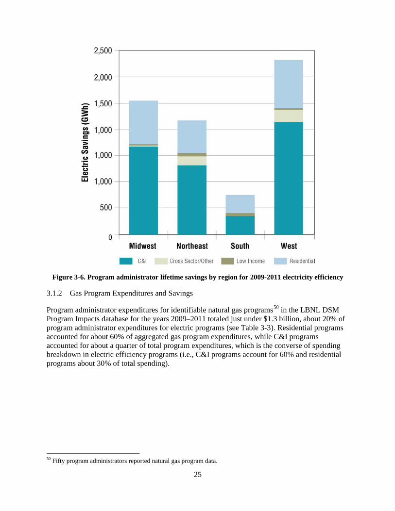
Figure 3-6. Program administrator lifetime savings by region for 2009-2011 electricity efficiency

3.1.2 Gas Program Expenditures and Savings

Program administrator expenditures for identifiable natural gas programs50 in the LBNL DSM Program Impacts database for the years 2009–2011 totaled just under $1.3 billion, about 20% of program administrator expenditures for electric programs (see Table 3-3). Residential programs accounted for about 60% of aggregated gas program expenditures, while C&I programs accounted for about a quarter of total program expenditures, which is the converse of spending breakdown in electric efficiency programs (i.e., C&I programs account for 60% and residential programs about 30% of total spending).

50 Fifty program administrators reported natural gas program data.

25

Figure 3-7. Program administrator expenditures, first- year and lifetime gross savings for 2009–

2011 natural gas efficiency programs

As with the residential sector programs, we compared the share of total program administrator expenditures with the share of first-year and lifetime savings for each market sector (see Figure 3-7). Expenditures for the C&I sector accounted for about a quarter of total gas program expenditures, yet C&I programs generated more than half of total gas program savings (56% of first-year savings and 62% of the lifetime gross savings), indicating the importance of this sector for natural gas energy efficiency.

Table 3-3. Program administrator expenditures for 2009-2011 natural gas efficiency programs

Market Sector Share of Total Program Administrator Expenditures

Total Program Administrator Expenditures (million 2012$)

Residential 58% $742

C&I 23% $291

Low Income 10% $123

Cross Sector/Other 9% $121

TOTAL 100% $1,277

On the other hand, while residential programs made up about 60% of total gas program expenditures, they garnered 35% of first-year savings and 40% of the total lifetime savings for all programs. Low income gas programs follow a similar pattern as low-income electricity efficiency programs, accounting for 10% of total expenditures and 6% of first-year and 5% lifetime savings.

26

3.2 Observations on the Cost of Saved Energy

3.2.1 National Observations

CSE values are presented as either (a) savings-weighted average values; (b) as an inter-quartile range with median51 values; or (c) both.52 The savings-weighted average CSE is calculated using all savings and expenditures at the level of analysis (e.g., region, sector, program category).53 For example, the national savings-weighted average CSE for the residential sector includes all the residential program portfolio costs in the database (even for programs without reported savings) divided by all the savings reported for the residential sector; thus “weighting” the CSE of larger programs more than small programs. The inter-quartile range and median CSE values are based on calculations for each individual program; thus giving equal weighting to all programs irrespective of their relative size (either in terms of savings or costs). The inter-quartile range and median CSE values exclude programs where a CSE cannot be calculated.54 CSE values are reported using three different metrics: a cost of lifetime saved energy, a levelized cost of energy savings using two discount rates (3% and 6% real), and a cost of first-year energy savings (see Table 2-2 for definitions of these CSE metrics). Appendix E contains detailed national and regional levelized CSE values by sector, simplified program type and detailed program type; tables in Appendix E show the savings-weighted average CSE, the first quartile, the median, and the third quartile levelized CSE values and the total number of programs for each category. Table 3-4 shows national saving-weighted average CSE values for the identifiable electricity efficiency programs55 in the database. Figure 3-8 depicts the lifetime and levelized CSE values ($/kWh) by sector. The national CSE values for electricity efficiency programs rounds to approximately $0.02/kWh for the levelized CSE using both the 3% and 6% real discount rates and a lifetime CSE (without discounting) of $0.015/kWh.

51 The inter-quartile range is the middle 50 percent of the range of program CSE values. The median is the numerical value separating the higher half of a data sample from the lower half. 52 The CSE values in this section are based on program administrator costs and gross energy savings. When used, the lifetime energy savings may be based on reported values or values derived from estimates of program average measure lifetime. See Chapter 2 for a discussion of the basis for using program administrator costs and gross savings, the protocol for calculating lifetime energy savings, and discussion of the limitations in the efficiency program data used to calculate CSE values. 53 We have observed that program administrators are not consistent in how they report program support costs (i.e. administration, EM&V, marketing & education, etc.). Some program administrators reported those costs at the program level, others reported those costs at the sector or portfolio level, and several reported those costs as, effectively, separate programs. For the purposes of this report, costs associated with specific programs stay associated with those programs. Costs that occur at the portfolio or sector levels are included in the analysis as separate programs. This allows us to account for those costs at the sector and portfolio levels but may appear as though individual programs within the same category cost less than their counterparts who report costs at the program level. 54 Some programs did not report savings (e.g., education/information programs) and others were not designed to achieve savings (i.e. programmatic support programs including EM&V, marketing). Where savings are not reported, it was not possible to calculate a CSE for that particular program. 55 Eighty-eight program administrators reported electric program data.

27

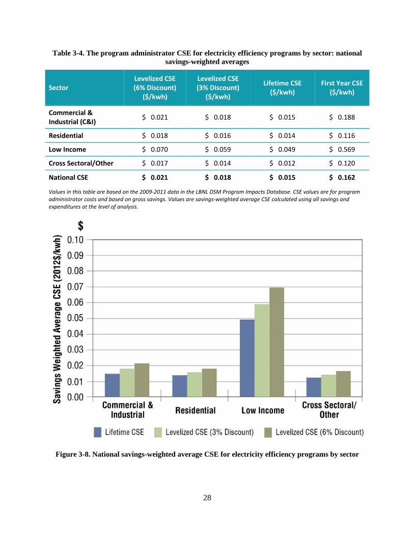
Table 3-4. The program administrator CSE for electricity efficiency programs by sector: national savings-weighted averages

Sector Levelized CSE (6% Discount)

($/kwh)

Levelized CSE (3% Discount)

($/kwh)

Lifetime CSE ($/kwh)

First Year CSE ($/kwh)

Commercial & Industrial (C&I) $ 0.021 $ 0.018 $ 0.015 $ 0.188

Residential $ 0.018 $ 0.016 $ 0.014 $ 0.116

Low Income $ 0.070 $ 0.059 $ 0.049 $ 0.569

Cross Sectoral/Other $ 0.017 $ 0.014 $ 0.012 $ 0.120

National CSE $ 0.021 $ 0.018 $ 0.015 $ 0.162

Values in this table are based on the 2009-2011 data in the LBNL DSM Program Impacts Database. CSE values are for program administrator costs and based on gross savings. Values are savings-weighted average CSE calculated using all savings and expenditures at the level of analysis.

Figure 3-8. National savings-weighted average CSE for electricity efficiency programs by sector

28

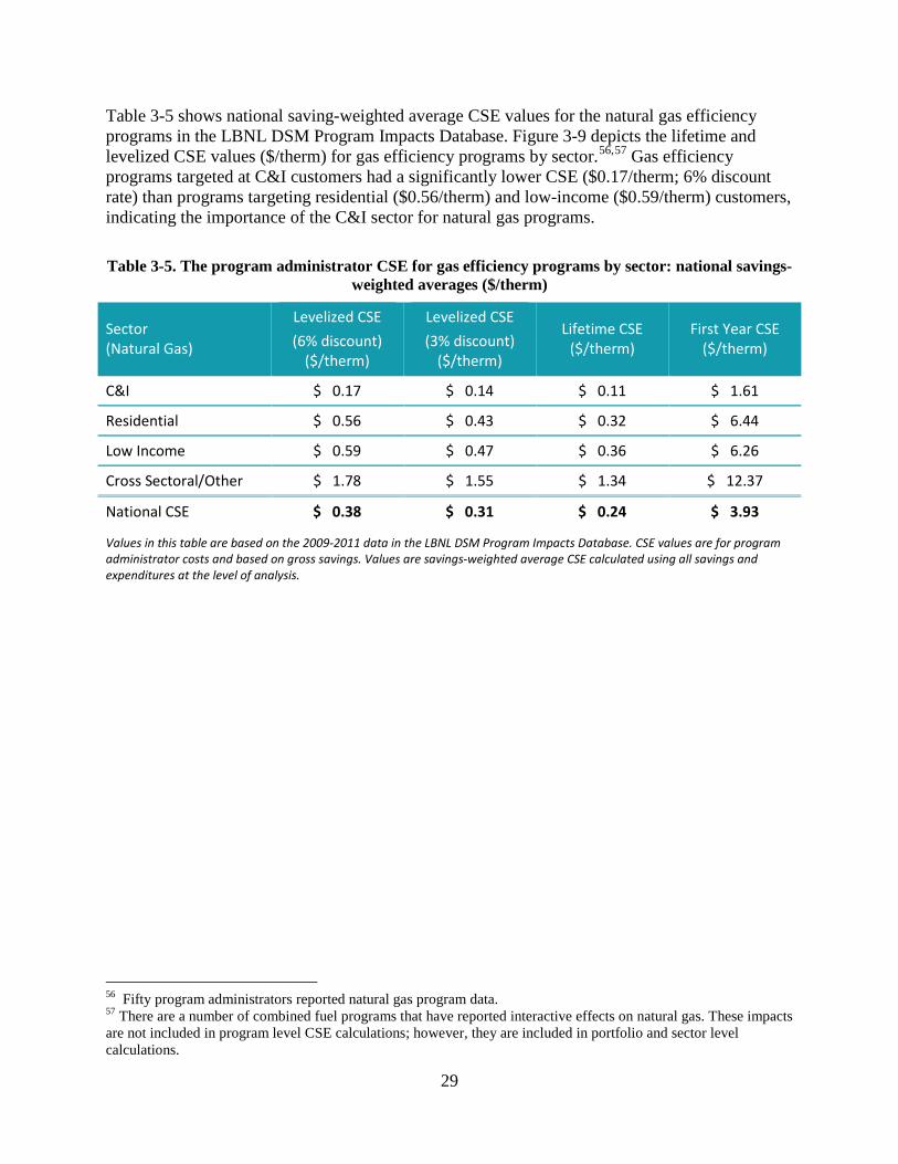
Table 3-5 shows national saving-weighted average CSE values for the natural gas efficiency programs in the LBNL DSM Program Impacts Database. Figure 3-9 depicts the lifetime and levelized CSE values ($/therm) for gas efficiency programs by sector.56,57 Gas efficiency programs targeted at C&I customers had a significantly lower CSE ($0.17/therm; 6% discount rate) than programs targeting residential ($0.56/therm) and low-income ($0.59/therm) customers, indicating the importance of the C&I sector for natural gas programs. Table 3-5. The program administrator CSE for gas efficiency programs by sector: national savings-

weighted averages ($/therm)

Sector (Natural Gas)

Levelized CSE (6% discount)

($/therm)

Levelized CSE (3% discount)

($/therm)

Lifetime CSE ($/therm)

First Year CSE ($/therm)

C&I $ 0.17 $ 0.14 $ 0.11 $ 1.61

Residential $ 0.56 $ 0.43 $ 0.32 $ 6.44

Low Income $ 0.59 $ 0.47 $ 0.36 $ 6.26

Cross Sectoral/Other $ 1.78 $ 1.55 $ 1.34 $ 12.37

National CSE $ 0.38 $ 0.31 $ 0.24 $ 3.93

Values in this table are based on the 2009-2011 data in the LBNL DSM Program Impacts Database. CSE values are for program administrator costs and based on gross savings. Values are savings-weighted average CSE calculated using all savings and expenditures at the level of analysis.

56 Fifty program administrators reported natural gas program data. 57 There are a number of combined fuel programs that have reported interactive effects on natural gas. These impacts are not included in program level CSE calculations; however, they are included in portfolio and sector level calculations.

29

Figure 3-9. CSE for natural gas efficiency programs by sector

3.2.2 Sector and Program Level Observations for Electricity Efficiency Programs

We present CSE values at the sector and program level in this section. For simplicity, the remainder of this chapter presents CSE values using the levelized CSE for a 6% (real) discount rate (except where otherwise indicated).58 Figure 3-10 presents the levelized CSE results on a national basis, depicting the savings-weighted average, median and inter-quartile range for each sector. We found that both C&I and residential electricity efficiency programs included in our database had an average levelized CSE of about $0.02/kWh. Looking at these sectors in more detail shows that the residential sector had a slightly lower weighted-average CSE than the commercial sector but a higher median CSE (~$0.04/kWh). The CSE values for residential sector programs also had a larger inter-quartile range than commercial sector programs (e.g., inter-quartile range of CSE values ran from just

58 We use a levelized CSE because we believe it is technically more appropriate for comparing resources. The 6% real discount rate is representative of a typical utility cost of capital. Lower discount rates result in lower CSE values. For example, for a program with an average measure life of 10 years for installed measures, a 6% discount rate results in a CSE that is about 15% higher than a 3% discount rate. There is significant interaction between discount rates and assumed measure lives. For example, the CSE value is 50% lower if we assume a 10 year measure life and 6% discount rate compared to a 20 year measure life and a 3% discount rate. See Appendix D for additional discussion of this issue.

30

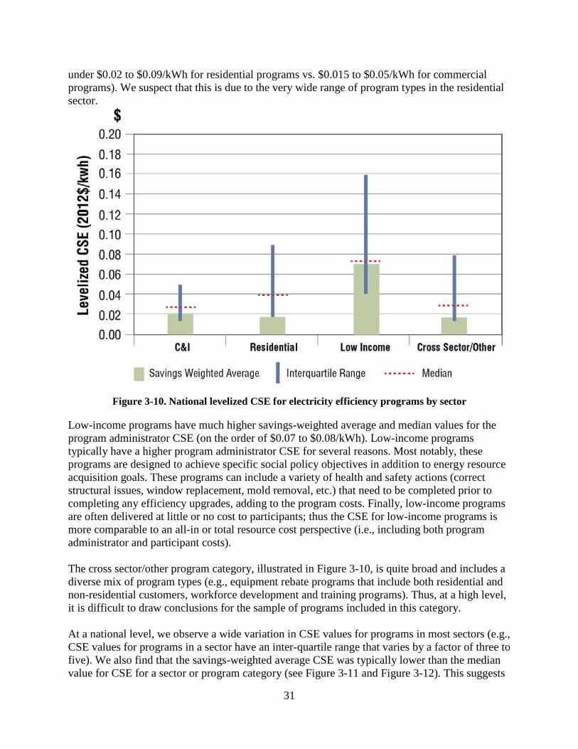
under $0.02 to $0.09/kWh for residential programs vs. $0.015 to $0.05/kWh for commercial programs). We suspect that this is due to the very wide range of program types in the residential sector.

Figure 3-10. National levelized CSE for electricity efficiency programs by sector

Low-income programs have much higher savings-weighted average and median values for the program administrator CSE (on the order of $0.07 to $0.08/kWh). Low-income programs typically have a higher program administrator CSE for several reasons. Most notably, these programs are designed to achieve specific social policy objectives in addition to energy resource acquisition goals. These programs can include a variety of health and safety actions (correct structural issues, window replacement, mold removal, etc.) that need to be completed prior to completing any efficiency upgrades, adding to the program costs. Finally, low-income programs are often delivered at little or no cost to participants; thus the CSE for low-income programs is more comparable to an all-in or total resource cost perspective (i.e., including both program administrator and participant costs). The cross sector/other program category, illustrated in Figure 3-10, is quite broad and includes a diverse mix of program types (e.g., equipment rebate programs that include both residential and non-residential customers, workforce development and training programs). Thus, at a high level, it is difficult to draw conclusions for the sample of programs included in this category. At a national level, we observe a wide variation in CSE values for programs in most sectors (e.g., CSE values for programs in a sector have an inter-quartile range that varies by a factor of three to five). We also find that the savings-weighted average CSE was typically lower than the median value for CSE for a sector or program category (see Figure 3-11 and Figure 3-12). This suggests

31

that much of the savings for each sector is coming from programs or program types on the low end of the CSE range for that program or sector. Figure 3-11 and Figure 3-12 show levelized CSE values for the simplified program categories for C&I and residential sectors, respectively.59 The simplified C&I program categories had median values for the program administrator’s CSE that range from $0.01/kWh to $0.05/kWh. It is worth noting that the savings-weighted average CSE for custom and prescriptive rebate program categories were $0.018/kWh and $0.015/kWh, respectively. Since these two program categories accounted for almost 70% of C&I sector savings (see Figure 3-4), they tended to drive the overall CSE results for the C&I sector: program administrators had an average levelized CSE of less than $0.02/kWh in the C&I sector. The C&I programs (Figure 3-11) also had a relatively smaller inter-quartile range of CSE values compared to the residential program categories (Figure 3-12).

Figure 3-11. National levelized CSE for commercial and industrial sector simplified program categories

59 Note that the y-axis scales for CSE are different in Figures 3-11 and 3-12, illustrating differences in the range of CSE values in C&I and residential sector programs.

32

Figure 3-12. National levelized CSE for residential sector simplified program categories

For the residential programs, several program categories had a relatively tight range of program administrator CSE values. For example, Consumer Product Rebate programs had an inter-quartile range of $0.01/kWh to nearly $0.04/kWh and a low savings-weighted average (~$0.01/kWh). However, the Residential Prescriptive ($0.03/kWh to $0.11/kWh), New Construction ($0.03/kWh to $0.11/kWh) and Whole-Home Upgrade (slightly more than $0.03/kWh to $0.21/kWh) program types had significantly larger ranges. There are several possible reasons for the larger range of CSE values in each of these program categories. The prescriptive simplified program category includes detailed program types that implement a wide variety of measures (e.g., HVAC, insulation, windows, pool pumps) as well as some generic “prescriptive” programs60 that often include measures also found in the Consumer Product Rebate category. This broad measure mix and the variation in costs and measure lifetimes associated with those measures are possible drivers for the wide range of CSE values for the prescriptive category.

60 Some programs include all their rebated measures under the same program title and it is not possible to determine where the majority of the savings is coming from. In these cases, the programs were categorized as “Residential Prescriptive.”

33

For the Whole-Home Upgrade program category, the broad range of program designs and delivery mechanisms (this category includes audit, direct install, and retrofit/upgrade programs) may help explain the relatively wide range of CSE values. Figure 3-1361 shows program administrator CSE values for detailed program categories under the Whole-Home Upgrade program category. We observe that the inter-quartile range of CSE values for both direct install and whole-home upgrade programs ranged from about $0.03/kWh to about $0.26/kWh, with median values of $0.06/kWh and $0.12/kWh, respectively. Whole home audit programs have a much smaller inter-quartile range, from $0.03/kWh to $0.11/kWh, and a median value of $0.07/kWh.

Figure 3-13. National levelized CSE for residential whole home detailed program category

Recall that about 44% of the residential sector lifetime gross savings came from lighting rebate programs that are part of the Consumer Product Rebate simplified program category (see Figure 3-13). Thus, we took a closer look at the CSE results for the four detailed program types within this category (see Figure 3-14). The median and average levelized CSE values for lighting rebate programs were quite low (about $0.01/kWh) with a small inter-quartile range (see Figure 3-14). Future investigation of these programs’ CSE values, savings estimates, and drivers is probably warranted given that a

61 Note that the y-axis scale in Figure 3-13 has higher CSE values than other figures in this chapter.

34

large percentage of savings came from lighting measures and that lighting CSE may rise as baselines (and thus perhaps savings) are lowered for many of these measures given implementation of more aggressive lighting equipment standards.

Figure 3-14. National levelized CSE for residential consumer product rebate detailed program categories

3.2.3 Regional Observations in Electricity Efficiency Programs

In this section, we examine some of the potential underlying drivers of CSE, including region (i.e., geographic location), climate, and baseline building efficiency requirements. Figure 3-15 presents regional CSE values for programs in the database (see Table 3-2 for assignment of states to region). Across all programs, the savings-weighted average CSE ($0.014/kWh) and median CSE ($0.019/kWh) values were lowest in the Midwest. This is consistent with the information in Figure 3-5 and Figure 3-6, which shows that program administrators in the Midwest in aggregate reported relatively low expenditures and relatively high savings (compared to other regions). Possible explanations for this phenomenon include the relative “newness” of the Midwest energy

35

efficiency programs and savings targets. Most of the states in this region enacted their first EERS targets in the late 2000s (Barbose et al. 2013). As a result, most of these states are perhaps still able to achieve significant savings from programs targeting low cost measures (i.e., lighting rebate programs). Another possible explanation is that gross savings values and/or measure lifetimes are higher because of baseline conditions or because EM&V practices are less mature in some states. In contrast, many states in the Northeast region have consistently been running efficiency programs for many years, have much higher savings targets (e.g., “all cost effective” efficiency mandates) and relatively well established and rigorous savings evaluation requirements. In aggregate, program administrators in the Northeast have a higher savings-weighted CSE ($0.033/kWh) and a much wider range of CSE values among types of programs, which possibly indicates that there was a broader mix of program designs and delivery mechanisms, as well as desire to achieve more comprehensive savings driven by state policy objectives (e.g., regulatory decisions or legislation that directs program administrators to achieve all cost-effective efficiency).

Figure 3-15. Levelized CSE for electricity efficiency programs by region

We also looked at average CSE values for all C&I and residential programs (excluding low-income programs) among program administrators in states (see Figure 3-16). Low-income programs were excluded for several reasons: (1) not all states either offer or reported information on their low-income programs; (2) the policy rationale(s) for low-income efficiency programs

36

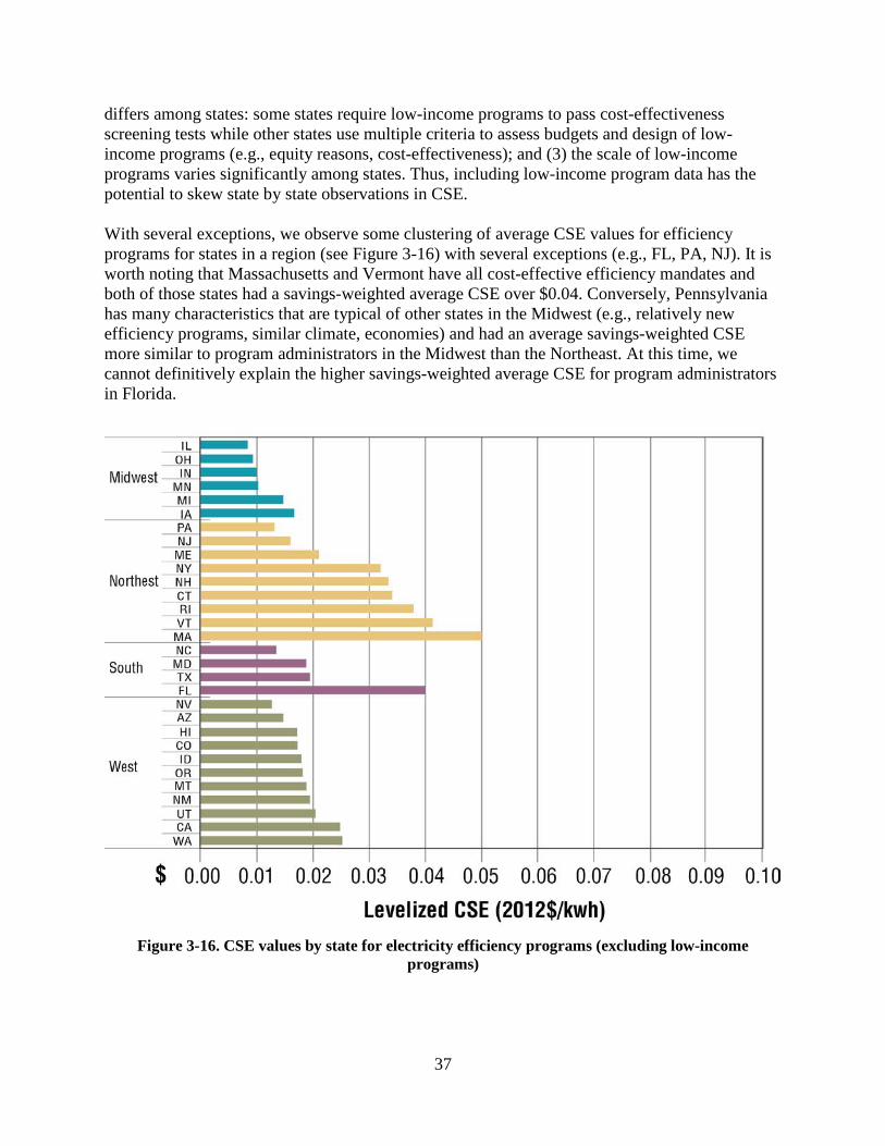
differs among states: some states require low-income programs to pass cost-effectiveness screening tests while other states use multiple criteria to assess budgets and design of low-income programs (e.g., equity reasons, cost-effectiveness); and (3) the scale of low-income programs varies significantly among states. Thus, including low-income program data has the potential to skew state by state observations in CSE. With several exceptions, we observe some clustering of average CSE values for efficiency programs for states in a region (see Figure 3-16) with several exceptions (e.g., FL, PA, NJ). It is worth noting that Massachusetts and Vermont have all cost-effective efficiency mandates and both of those states had a savings-weighted average CSE over $0.04. Conversely, Pennsylvania has many characteristics that are typical of other states in the Midwest (e.g., relatively new efficiency programs, similar climate, economies) and had an average savings-weighted CSE more similar to program administrators in the Midwest than the Northeast. At this time, we cannot definitively explain the higher savings-weighted average CSE for program administrators in Florida.

Figure 3-16. CSE values by state for electricity efficiency programs (excluding low-income

programs)

37

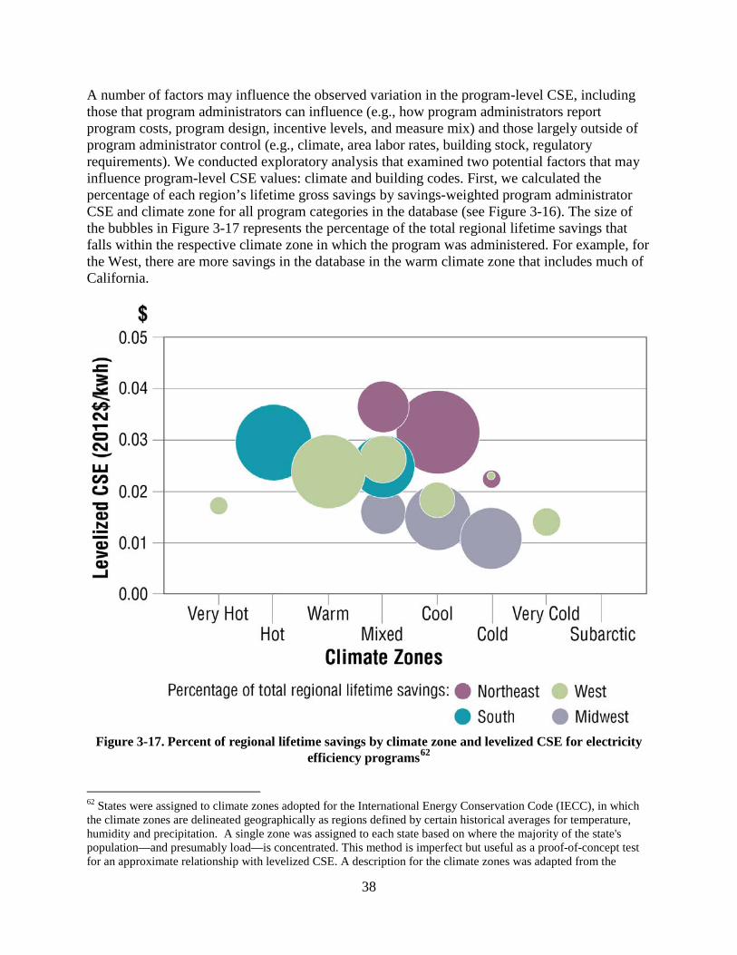
A number of factors may influence the observed variation in the program-level CSE, including those that program administrators can influence (e.g., how program administrators report program costs, program design, incentive levels, and measure mix) and those largely outside of program administrator control (e.g., climate, area labor rates, building stock, regulatory requirements). We conducted exploratory analysis that examined two potential factors that may influence program-level CSE values: climate and building codes. First, we calculated the percentage of each region’s lifetime gross savings by savings-weighted program administrator CSE and climate zone for all program categories in the database (see Figure 3-16). The size of the bubbles in Figure 3-17 represents the percentage of the total regional lifetime savings that falls within the respective climate zone in which the program was administered. For example, for the West, there are more savings in the database in the warm climate zone that includes much of California.

Figure 3-17. Percent of regional lifetime savings by climate zone and levelized CSE for electricity

efficiency programs62

62 States were assigned to climate zones adopted for the International Energy Conservation Code (IECC), in which the climate zones are delineated geographically as regions defined by certain historical averages for temperature, humidity and precipitation. A single zone was assigned to each state based on where the majority of the state's population—and presumably load—is concentrated. This method is imperfect but useful as a proof-of-concept test for an approximate relationship with levelized CSE. A description for the climate zones was adapted from the

38

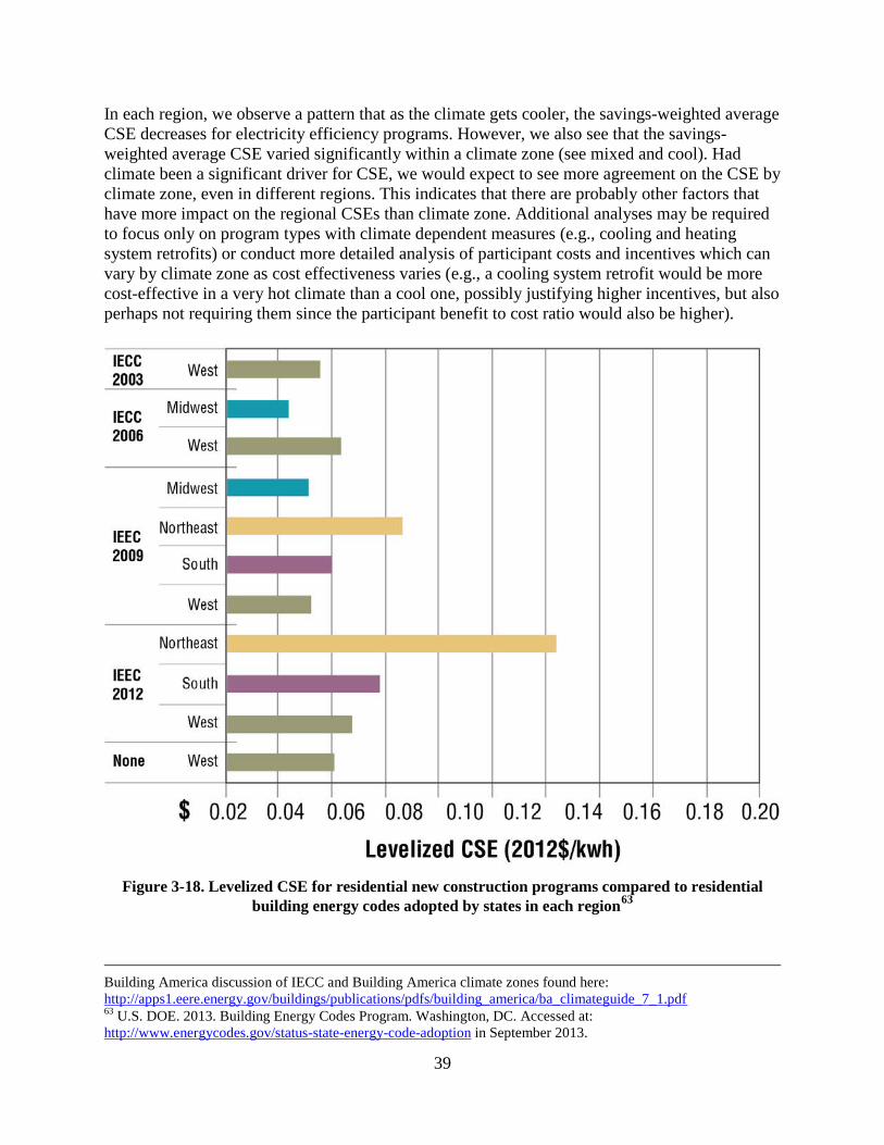
In each region, we observe a pattern that as the climate gets cooler, the savings-weighted average CSE decreases for electricity efficiency programs. However, we also see that the savings-weighted average CSE varied significantly within a climate zone (see mixed and cool). Had climate been a significant driver for CSE, we would expect to see more agreement on the CSE by climate zone, even in different regions. This indicates that there are probably other factors that have more impact on the regional CSEs than climate zone. Additional analyses may be required to focus only on program types with climate dependent measures (e.g., cooling and heating system retrofits) or conduct more detailed analysis of participant costs and incentives which can vary by climate zone as cost effectiveness varies (e.g., a cooling system retrofit would be more cost-effective in a very hot climate than a cool one, possibly justifying higher incentives, but also perhaps not requiring them since the participant benefit to cost ratio would also be higher).

Figure 3-18. Levelized CSE for residential new construction programs compared to residential

building energy codes adopted by states in each region63

Building America discussion of IECC and Building America climate zones found here: http://apps1.eere.energy.gov/buildings/publications/pdfs/building_america/ba_climateguide_7_1.pdf 63 U.S. DOE. 2013. Building Energy Codes Program. Washington, DC. Accessed at: http://www.energycodes.gov/status-state-energy-code-adoption in September 2013.

39

http://apps1.eere.energy.gov/buildings/publications/pdfs/building_america/ba_climateguide_7_1.pdf

http://www.energycodes.gov/status-state-energy-code-adoption

Another potential influence on CSE values is differences in baseline building efficiency across states and regions. In Figure 3-18 and Figure 3-19, we examine the savings-weighted average CSE for new construction programs in the residential and commercial sectors, respectively. For the residential programs, we calculate the savings-weighted average electric levelized CSE for new construction programs in each region plotted against each state’s current International Energy Conservation Code (IECC) status.64,65 The newer the adopted code, the lower the assumed baseline energy consumption, which tends to reduce the incremental electricity savings for any given efficiency action. For example, the gross savings calculated for a fixed set of measures for a building than meets the 2006 IECC code would be greater than for the same set of measures for a building that meets the 2012 IECC code. Note that the West, as a region, has the most diversity among states in terms of building energy code requirements.

Figure 3-19. Regional levelized CSEs for commercial new construction programs compared to

commercial building energy codes adopted by states in each region66

64 The IECC (http://www.iccsafe.org/gr/Pages/IECC-Resource.aspx) is a national model energy code for the United States. It sets minimum requirements for energy efficiency that new buildings—as well as additions and renovations to existing buildings—must meet wherever the code has been adopted into law, usually on state-by-state basis. The IECC is updated on a 3-year cycle, and the most recent version is 2012. 65 By using current (2103) IECC code adoption status, we do not directly reflect the baseline status at time of program implementation (2009-2011). However, we expect that this approach may still be indicative of relative baseline status while not requiring state-by-state, year-by-year analysis of code status. 66 U.S. DOE. 2013. Building Energy Codes Program. Washington, DC. Accessed at: http://www.energycodes.gov/status-state-energy-code-adoption in September 2013.

40

http://www.iccsafe.org/gr/Pages/IECC-Resource.aspx

http://www.energycodes.gov/status-state-energy-code-adoption

It might be reasonable to expect that the CSE would increase as the codes for new buildings set more stringent baseline efficiency requirements (e.g., incremental savings opportunities are less for any given investment). Some evidence for this pattern can be observed in the average CSE values for Midwest, Northeast and South residential programs segmented by the year of the building energy codes. However, the expected pattern in average CSE values does not readily emerge for states in the West that offer residential new construction programs.

The picture is even less clear when looking at the savings-weighted CSE for commercial new construction programs plotted against commercial codes (see Figure 3-19). CSE values do not follow the expected pattern for states in either the West or Midwest. The savings-weighted average CSE values for states in the Northeast seems to have been lower where more stringent codes exist, although there are a limited range of code requirements among states in the Northeast. Thus, the effects of code status on CSE values require further inquiry. 3.2.4 Sensitivity Analysis: Impact of Measure Lifetime

In Chapter 2, we discussed data gaps and inconsistent criteria for reporting lifetime energy savings (and by extension efficiency measure lifetimes), noting that lifetime savings (or program average measure lifetime) were not reported for about 50% of the program years in the database.67 In this section, we illustrate and discuss results of a sensitivity analysis that explores the impact of varying assumptions regarding program measure lifetime on CSE values reported by program administrators. Figure 3-20 compares the “LBNL approach” used to estimate lifetime savings for those programs that did not report this information to two other potential approaches in which we apply the minimum and maximum reported program average lifetimes for each detailed program type to all programs of that type. The minimum and maximum values for each program type (see the light and dark green bars in Figure 3-20) dramatize the impact on levelized CSE values of varying assumptions for the average measure lifetime of efficiency programs. For five of the 12 reported program categories, if we use the minimum reported program average lifetime (and apply it to all other programs in that category), the levelized CSE values more than doubles compared to the CSE values using the LBNL measure lifetime approach. This underscores the importance of understanding and accurately reporting the average measure lifetime of measures installed in programs since it significantly impacts the cost of saved energy (and the underlying cost-effectiveness of efficiency actions).

67 For those programs, we calculated a program-average measure lifetime by detailed program category and applied those values to the reported gross first-year savings to calculate lifetime savings.

41

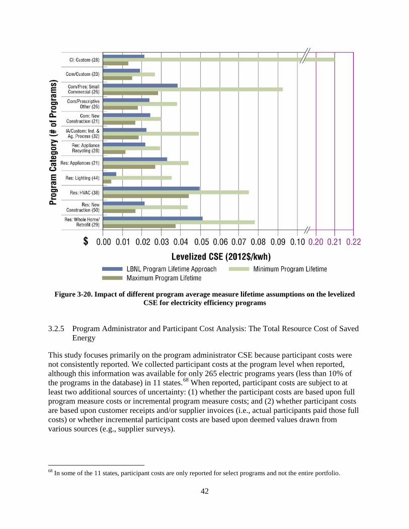
Figure 3-20. Impact of different program average measure lifetime assumptions on the levelized CSE for electricity efficiency programs

3.2.5 Program Administrator and Participant Cost Analysis: The Total Resource Cost of Saved

Energy

This study focuses primarily on the program administrator CSE because participant costs were not consistently reported. We collected participant costs at the program level when reported, although this information was available for only 265 electric programs years (less than 10% of the programs in the database) in 11 states.68 When reported, participant costs are subject to at least two additional sources of uncertainty: (1) whether the participant costs are based upon full program measure costs or incremental program measure costs; and (2) whether participant costs are based upon customer receipts and/or supplier invoices (i.e., actual participants paid those full costs) or whether incremental participant costs are based upon deemed values drawn from various sources (e.g., supplier surveys).

68 In some of the 11 states, participant costs are only reported for select programs and not the entire portfolio.

42

Given small sample size and uncertain reporting of participant costs, it is difficult to assess the “all-in” or total resource cost of efficiency or analyze potential influences on the total cost of the efficiency resource. For these reasons, in Figure 3-21, we compare the program administrator’s levelized CSE vs. a total resource CSE for illustrative purposes only. We calculate this total resource CSE for the simplified program categories where both program administrator and participant costs were available for more than 18 program years.69 For the small sample of programs, we found that the levelized total resource CSE values are typically double for most program types with the exception of the Residential Whole Home Upgrade program category (where the total resource CSE is about 25%–30% higher than the program administrator CSE). Further data collection and analyses could help understand how the ratio of program administrator to participant costs varies as a function of sector, measure types, and market maturity; and how incentives and direct support might be optimized to pay no more than is necessary to meet efficiency uptake objectives.

Figure 3-21. Levelized savings-weighted average CSE for electricity efficiency programs that include program administrator costs vs. total resource costs for select program categories70

69 The “n” of 18 was selected because there was a natural break in the data and also that criteria resulted in only including results for which there was a meaningful number of programs from which to calculate average values. 70 This chart includes a very small sample of programs from 11 states; thus, results may not reflect current practices in many jurisdictions.

43

4. Testing Influences on the Costs of Saved Energy

As shown in Chapter 3, we observe a wide range of values for the program administrator CSE from virtually every perspective—nationally, and across regions, states, portfolios, and sectors. Moreover, we find significant variability within the different types of programs. The inter-quartile range of CSE values (the “middle” 50% of programs) for the first-year CSE can vary by a factor of 10 or more within a program category. In this chapter, we explore some factors that may be associated with this variability in the CSE. We describe the results of statistical analyses aimed at quantifying the relationship of CSE and a few, selected independent variables. To initiate these analyses, we postulated three sets of potential explanations for these ranges of CSE values:

• Differences internal to the programs themselves and over which program administrators have at least some influence (e.g., the mix of measures in programs and thus the adoption patterns of consumers, the scale of programs, the maturity of the programs, program design, and program implementation);

• Differences external to the programs and over which program administrators have very little or no influence (e.g., climate, labor costs, and the policy framework within which programs operate).

• Incorrect information arising from problems with the primary data or faulty categorization of programs, or both (e.g., if gross energy savings are inaccurately reported in the source reports).71

We suspect that most or all of these factors influence the CSE values, interacting in ways that can be difficult to disentangle. In this chapter, we focus on the first two explanations (i.e., potential internal and external program influences) in order to see if their hypothesized influences on CSE are observed or not, using the programs in the database.72 In the long run, we hope the collected data and this type of statistical analyses can:

• Inform policymakers and other stakeholders about the variability of the CSE to distinguish between controllable and uncontrollable sources of variability and, ideally, to identify ways of reducing costs or otherwise improving program design and delivery; and

• Lead to predictive models that specify and quantify major influences on CSE values and thus could inform cost or savings projections for use by portfolio planners, regulators, and resource planners.

71 See Chapter 2 for a discussion of data issues and Appendix C for a description of the quality control procedures implemented for this project. 72 As noted in Chapter 3, CSE values are derived as follows: Program costs refer to program administrator costs only; the CSE values exclude participant costs. Savings are gross savings as reported by the program administrator. When program administrators only reported net savings values and we either had or could derive program-specific net-to-gross ratios, we used those ratios to calculate gross savings values from reported net savings. Savings values are based on savings at the end-use site and not at the power plant or natural gas pumping station and thus do not account for transmission and distribution losses.

44

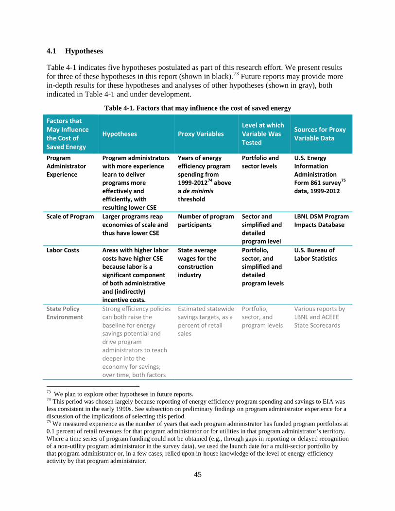
4.1 Hypotheses

Table 4-1 indicates five hypotheses postulated as part of this research effort. We present results for three of these hypotheses in this report (shown in black).73 Future reports may provide more in-depth results for these hypotheses and analyses of other hypotheses (shown in gray), both indicated in Table 4-1 and under development.

Table 4-1. Factors that may influence the cost of saved energy

Factors that May Influence the Cost of Saved Energy

Hypotheses Proxy Variables Level at which Variable Was Tested

Sources for Proxy Variable Data

Program Administrator Experience

Program administrators with more experience learn to deliver programs more effectively and efficiently, with resulting lower CSE

Years of energy efficiency program spending from 1999-201274 above a de minimis threshold

Portfolio and sector levels

U.S. Energy Information Administration Form 861 survey75 data, 1999-2012

Scale of Program Larger programs reap economies of scale and thus have lower CSE

Number of program participants

Sector and simplified and detailed program level

LBNL DSM Program Impacts Database

Labor Costs

Areas with higher labor costs have higher CSE because labor is a significant component of both administrative and (indirectly) incentive costs.

State average wages for the construction industry

Portfolio, sector, and simplified and detailed program levels

U.S. Bureau of Labor Statistics

State Policy Environment

Strong efficiency policies can both raise the baseline for energy savings potential and drive program administrators to reach deeper into the economy for savings; over time, both factors

Estimated statewide savings targets, as a percent of retail sales

Portfolio, sector, and program levels

Various reports by LBNL and ACEEE State Scorecards

73 We plan to explore other hypotheses in future reports. 74 This period was chosen largely because reporting of energy efficiency program spending and savings to EIA was less consistent in the early 1990s. See subsection on preliminary findings on program administrator experience for a discussion of the implications of selecting this period. 75 We measured experience as the number of years that each program administrator has funded program portfolios at 0.1 percent of retail revenues for that program administrator or for utilities in that program administrator’s territory. Where a time series of program funding could not be obtained (e.g., through gaps in reporting or delayed recognition of a non-utility program administrator in the survey data), we used the launch date for a multi-sector portfolio by that program administrator or, in a few cases, relied upon in-house knowledge of the level of energy-efficiency activity by that program administrator.

45

are likely to result in higher CSE.

Retail Rate Environment

Higher retail energy costs result in lower CSE because the higher energy costs encourage more customers to invest in energy savings, thus lowering the program administrator’s costs of securing participation and savings

Residential, commercial and industrial retail rates

Commercial and Industrial (C&I) and residential sectors

U.S. EIA 826 and 861 reports (the Monthly Electric Sales and Revenue Report with State Distributions Report and the Annual Electric Power Industry Report)

Through the exercise of developing the hypotheses and identifying associated independent variables, it became clear that several of our theorized influences on the CSE interact in complex ways. Several variables operate in synergistic or countervailing ways. For example, some policies that are generally supportive of saving energy (e.g., energy savings targets) may dampen the costs of saving energy for program administrators in some circumstances and yet increase those costs under other circumstances. Further, the resulting effects may not operate uniformly or in the same direction from one market sector to another or across program types. Thus, the identification of potential influences on the CSEs, development of testable hypotheses and identification of valid independent variables is an iterative process, the early phases of which are described below. 4.2 Approach

For our dependent variable, we chose the first-year electric CSE, which is simply the program administrator cost (2012$) divided by first-year gross electricity savings (in kWh). The primary advantage of using first-year savings (versus lifetime savings) is eliminating uncertainties associated with the measure lifetime data; see Chapters 2 and 3 for discussion of limitations of lifetime energy savings data. The disadvantage of using first-year savings is the inability to examine the ways that potential influences on CSEs vary for shorter- versus longer-lived efficiency measures, as using a levelized or lifetime CSE might allow. Since energy resources are generally evaluated over their economic lifetime, we anticipate analyzing factors that may be associated with levelized CSE values. We identified and collected data on the independent variables as proxies for the factors chosen to represent the potential influences over CSE. We then performed single-variable ordinary least squares regressions to screen independent variables, followed by a limited number of multivariate regressions to test the correlation between variables and the relative contributions of the variables. Appendix F describes our data collection procedures for the independent variables, the statistical analysis process and contains a table of these preliminary regression results.

Statistical Regressions

Statistical regressions do not necessarily imply causality. Regressions can establish correlation or a probability that changing one or more independent variables is significantly associated with a quantifiable change in the dependent variable (e.g., the CSE).

46

4.3 Preliminary Results: Analysis of Factors that May Influence the Cost of Saved Energy

Our preliminary results to date suggest that many factors influence the CSE, and the degree of those influences varies across market sectors and programs. In the following subsections, we present an illustrative sampling of preliminary results and also discuss some of the challenges in identifying valid independent variables and interpreting results. 4.3.1 Program Administrator Experience

We hypothesized that program administrators with more experience would, to some demonstrable degree, have optimized the efficacy of program implementation and thus have lower CSE values for their portfolio of programs after an initial period. Experienced program administrators might realize these cost savings by one or more mechanisms, including having already established the necessary program infrastructure and trade alliances, identifying cost efficiencies in overhead expenses, and learning what measures and marketing approaches tend to elicit more customer participation or deeper savings. We defined the program administrator experience variable as follows: each year of spending above a minimum program spending threshold (0.1% of revenues) as reported to the Energy Information Administration counted as a year of experience administering efficiency programs.76 Years of experience were summed up for all years where spending exceeded the threshold to the program year for the data being tested. For example, utility X offered an informational energy audit program to customers in 2004 and expanded their programs in subsequent years such that spending exceeded 0.1% of revenues in 2006. Thus, we assumed that this utility had four years of experience for their 2010 programs and five years of experience for their 2011 programs. The nature of the relationship between first-year CSE values and program administrator experience is depicted in Figure 4-1. The blue dots in Figure 4-1 represent CSE values for the portfolio of programs offered each year by individual program administrators. The cost of first-year gross electricity savings is plotted on the y-axis, the years of program administrator experience are shown on the x-axis. There may be a quadratic relationship, such that program administrator experience and the cost of first-year savings may trace a curve in which first-year CSE declines as program administrators gain experience and then, beyond a certain number of years, costs increase, as

76 See Appendix F for a more detailed explanation of the basis for determining program administrator years of experience. Response rates vary among program administrators from year to year in providing EIA Form-861 information. Third-party program administrators were not included in the EIA datasets until very recently. The names and parent companies for some program administrators changed over time. Some EIA survey data terms and definitions have changed over time and program administrators may have interpreted those terms (e.g., direct vs. indirect spending) in different ways. These limitations increase as the data reaches back to the early years of the EIA survey. We therefore chose to limit the count of years above the spending threshold to a period from 1999 to 2012. We recognize that bounding our metric for program administrator experience to this 14-year period imposes an artificial ceiling on the level of experience for the most mature program administrators. This may affect the correlation between program administrator maturity and the cost of saved energy. However, this impact is likely to be limited because 80% of the program administrator s in our dataset have spent above the designated spending threshold for 10 or fewer years.

47

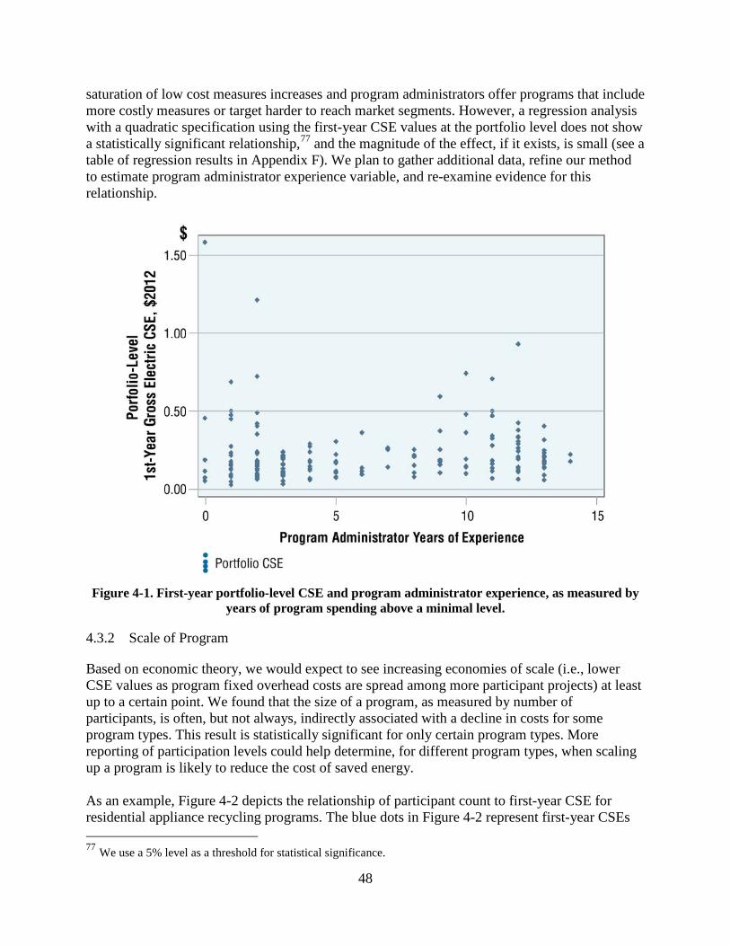
saturation of low cost measures increases and program administrators offer programs that include more costly measures or target harder to reach market segments. However, a regression analysis with a quadratic specification using the first-year CSE values at the portfolio level does not show a statistically significant relationship,77 and the magnitude of the effect, if it exists, is small (see a table of regression results in Appendix F). We plan to gather additional data, refine our method to estimate program administrator experience variable, and re-examine evidence for this relationship.

Figure 4-1. First-year portfolio-level CSE and program administrator experience, as measured by

years of program spending above a minimal level.

4.3.2 Scale of Program

Based on economic theory, we would expect to see increasing economies of scale (i.e., lower CSE values as program fixed overhead costs are spread among more participant projects) at least up to a certain point. We found that the size of a program, as measured by number of participants, is often, but not always, indirectly associated with a decline in costs for some program types. This result is statistically significant for only certain program types. More reporting of participation levels could help determine, for different program types, when scaling up a program is likely to reduce the cost of saved energy. As an example, Figure 4-2 depicts the relationship of participant count to first-year CSE for residential appliance recycling programs. The blue dots in Figure 4-2 represent first-year CSEs

77 We use a 5% level as a threshold for statistical significance.

48

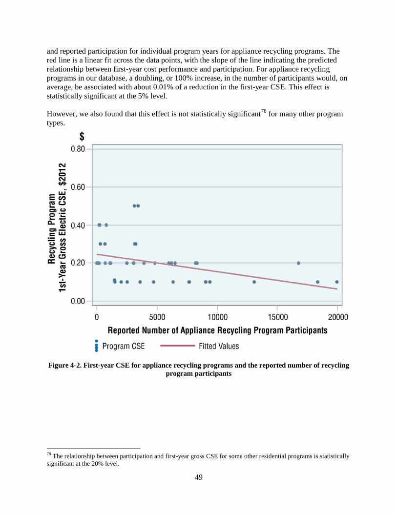
and reported participation for individual program years for appliance recycling programs. The red line is a linear fit across the data points, with the slope of the line indicating the predicted relationship between first-year cost performance and participation. For appliance recycling programs in our database, a doubling, or 100% increase, in the number of participants would, on average, be associated with about 0.01% of a reduction in the first-year CSE. This effect is statistically significant at the 5% level. However, we also found that this effect is not statistically significant78 for many other program types.

Figure 4-2. First-year CSE for appliance recycling programs and the reported number of recycling

program participants

78 The relationship between participation and first-year gross CSE for some other residential programs is statistically significant at the 20% level.

49

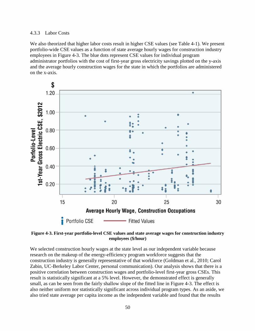
4.3.3 Labor Costs

We also theorized that higher labor costs result in higher CSE values (see Table 4-1). We present portfolio-wide CSE values as a function of state average hourly wages for construction industry employees in Figure 4-3. The blue dots represent CSE values for individual program administrator portfolios with the cost of first-year gross electricity savings plotted on the y-axis and the average hourly construction wages for the state in which the portfolios are administered on the x-axis.

Figure 4-3. First-year portfolio-level CSE values and state average wages for construction industry

employees ($/hour)

We selected construction hourly wages at the state level as our independent variable because research on the makeup of the energy-efficiency program workforce suggests that the construction industry is generally representative of that workforce (Goldman et al., 2010; Carol Zabin, UC-Berkeley Labor Center, personal communication). Our analysis shows that there is a positive correlation between construction wages and portfolio-level first-year gross CSEs. This result is statistically significant at a 5% level. However, the demonstrated effect is generally small, as can be seen from the fairly shallow slope of the fitted line in Figure 4-3. The effect is also neither uniform nor statistically significant across individual program types. As an aside, we also tried state average per capita income as the independent variable and found that the results

50

are similar to those using construction hourly wages; this seems to indicate that labor costs are likely to play some role in the cost of saving energy. 4.4 Analytical Challenges

We also conducted exploratory analysis of other hypotheses (e.g., policy and retail price environments in which programs operate) and found that results varied substantially by market sector and program type. Many of these theorized relationships with the CSE are significant only at the 10%-15% level; further study is warranted. The statistical analysis results described in this chapter depend critically on defining valid independent variables as well as the quality and quantity of the primary data underlying both the independent and dependent variables. Some of the difficulty in parsing these effects is a function of limitations in the underlying data for the independent variables. Drawing on an example noted earlier, we used data that program administrators voluntarily reported to the Energy Information Agency (EIA) to develop proxies for years of administrator experience. Program administrators sometimes do not report spending for every year or have interpreted EIA survey questions in different ways. More work is needed to minimize these and other sources of error or uncertainty in values for the independent variables. Another challenge is specifying independent variables that are not highly correlated with other variables, that is, some proxies for influences on CSE can be overlapping in effect. For example, program administrators with more experience usually are required to achieve higher levels of savings. States that have higher labor costs also often have higher retail rates. Likewise, it can be difficult to examine economies-of-scale questions when participation data are not provided. No participation data are reported for more than two-thirds of the program years in the database. In other cases, the data may be incorrect (numbers identified as participants are actually units sold or assumed installed) or ambiguous (unit and participant numbers are co-mingled or undifferentiated). Finally, many other questions pertinent to program design and delivery could be tested if spending breakdowns were available by program (i.e., program expenditures disaggregated into customer incentives, various categories of administration, marketing and outreach, and evaluation). The primary data contained in the database have limitations, as discussed earlier. For the regression analysis, our total sample size was 2,035 data points. Many of the program years in the database are for gas-only programs, which are not included in an analysis of electricity program CSEs. Moreover, for some programs, the administrator did not report a key value (e.g., did not include program-level spending or allocate program costs by fuel for combination electric-gas programs).

51

5. Discussion of Key Findings and Recommendations

In this chapter, we summarize key findings from this initial report of the LBNL CSE Project and discuss opportunities for improving information provided by program administrators on the costs and impacts of efficiency programs. 5.1 Key Findings

We calculated the administrator costs of saving a unit of natural gas or electricity and reported the CSE in several ways, through first-year savings, lifetime savings and levelized savings. It is important to note that the CSE values presented in this report are retrospective and may not necessarily reflect future CSE for specific programs, particularly given updated appliance and lighting standards. The cost of efficiency as a function of first-year energy savings may be useful for budgeting to meet incremental annual savings targets. The cost of lifetime energy savings captures the efficiency that accrues throughout the effective lifetime of the implemented measures and therefore is more broadly applicable in designing programs and portfolios. In this study, we focused more attention on the program administrators’ levelized cost of energy savings based on gross savings because relatively few program administrators reported the cost contributions of participants (or incremental measure costs) or net savings values. In future reports, our goals are to also provide the “all-in” or total resource CSE and to include CSE values based on net savings as well. Key findings from this study are:79

• The U.S. average electricity CSE was slightly more than two cents per kilowatt-hour in the period 2009-2011 when gross savings and spending are aggregated at the national level and the CSE is weighted by savings.80 This levelized CSE is somewhat lower than reported by other previous studies. In a 2009 study, for example, Friedrich et al. found an average program administrator levelized CSE of $0.025/kWh in constant 2007 dollars or $0.027/kWh in constant 2012 dollars—about 29% higher than is reported here.81 The LBNL DSM Program Impacts Database contains a larger sample of program administrators, many of whom may have used longer program measure lifetimes that could affect CSE values. Moreover, nearly 40% of the program administrators in the database that administer electric efficiency programs have offered programs for less than four years and so may be early in accessing energy savings in their respective state economies or be targeting the least costly savings opportunities first.82

• Other findings for electricity efficiency programs include:

79 All values reported here are program administrator CSEs for gross energy savings, levelized at a 6% real discount rate and given in constant 2012 dollars. 80 This average value is based on the efficiency program portfolios of 100 electric and electric-gas program administrators that represent just less than half of the program spending in the United States during 2009 through 2011. These PAs are a large and diverse group in terms of geography, baseline efficiency, and historic levels of program activity. 81 Friedrich et al. used a slightly lower discount rate (5 percent vs. 6 percent used in this report), so that the actual difference is larger. 82 See Appendix A for summary of current and previous CSE research.

52

o Residential electricity efficiency programs had the lowest average levelized CSE at $0.018/kWh. Commercial, industrial and agricultural (C&I) programs had a slightly higher average levelized CSE at $0.021/kWh. Low-income programs show an average levelized CSE at $0.070/kWh.

o In reviewing regional results, the Midwest programs had the lowest average levelized CSE ($0.014/kWh) and the Northeast programs the highest ($0.033/kWh). The average levelized CSE values for programs in the West and South, to the extent sufficient reporting was found, were $0.023/kWh and $0.028/kWh, respectively.

o The database provides a valuable resource for understanding the composition and the CSE for various efficiency measures and program types. For example, at least 44% of the reported gross savings in the residential sector came from dedicated lighting programs and lighting rebate programs had a savings-weighted average CSE of $0.007/kWh with a small inter-quartile range.

• Natural gas efficiency programs had a national, program administrator savings weighted CSE range of $0.24 (lifetime CSE) to $0.38 per therm (levelized CSE, 6% discount rate), with significant differences between the commercial/industrial and residential sectors ($0.11–$0.17 vs. $0.32–$0.56 per therm respectively).

• Not surprisingly, the levelized CSE varied widely both among program types and within program types. We found that the median value was typically higher than the savings-weighted average for nearly all types of programs. One possible explanation is that our sample includes a number of very large programs and for any given program type, larger efficiency programs have lower CSE than smaller programs because administrative costs are spread over more projects (e.g., economies of scale). Some of our statistical analyses tend to demonstrate this relationship; however, other factors are probably at work as well.

• The “all-in” or total resource cost of energy savings is subject to the uncertainties and very limited availability of information on participant costs. Based on our small sample of programs that reported participant costs, we found that the program administrator costs account for about a third to a half of the total CSE (including program administrator and participant costs). One exception is residential Whole-Home Upgrade programs in our database, for which the median value for the program administrator’s CSE is closer to three-quarters of the median CSE value that includes both program administrator and participant costs.

• We developed several hypotheses regarding factors that may influence the variability in the cost of saved energy. Preliminary statistical analyses of cost of first year energy savings suggest that myriad factors both internal and external to program design and implementation play some role in influencing the CSE: o Program administrator experience and the cost of first-year savings may show a

curve where first-year CSE declines as new program administrators gain experience and then, beyond a certain number of years, costs increase, consistent with administration of portfolios that have matured beyond acquiring the least expensive resources. However, the demonstrated effect is generally small and not statistically significant at this time.

53

o Higher construction labor costs are associated with higher costs of energy savings at the portfolio level. However, the demonstrated effect is generally small and is not uniform (or statistically significant) across all types of programs.

o The size of a program, as measured by the number of participants, is associated with a decline in costs for some types of programs, suggesting that certain programs (e.g., Appliance Recycling programs) can achieve economies of scale by spreading fixed overhead across more projects. However, we also found that this result is not statistically significant for many other types of efficiency programs. More reporting of participation data could help determine when scaling up a program is likely to reduce costs and for what program types.

5.2 Discussion: Program Data Collection and Reporting

Program administrator annual reports are typically the product of state regulatory requirements or traditional practices that have evolved over time. In compiling and analyzing more than 4,000 program-years of data, we discovered a wide spectrum in the level of detail and completeness in annual program reporting. Barbose et al. (2013) found that over 45 states are running utility customer-funded efficiency programs. Many program administrators report program-level data at a very high level of completeness and transparency. However, we also found many examples of annual reports from program administrators that do not provide a complete picture of the impacts or costs of the efficiency investments at the program level. Although these reports may meet regulatory requirements in their state, they were not sufficient for the purposes of CSE analysis and therefore we were not able to include results from program administrators in many states. With respect to current program reporting practices, we found:

• Inconsistencies in the quality and quantity of the costs and savings data which led LBNL to develop and attempt to apply consistent data definitions in reviewing and entering program data: o Program administrators in different states did not define savings metrics (e.g.,

varying definitions of net savings) and program costs consistently; and o Market sectors and program types were not characterized in a consistent fashion

among program administrators. • Many program administrators did not provide the basic data needed to calculate a

CSE at the program level (i.e., program administrator costs and annual and lifetime savings), which introduced uncertainties into the calculation of CSE values.

This project brought into sharp relief the challenges of creating a program spending and savings database and calculating reliable, internally consistent metrics for assessing programmatic energy efficiency. For example, program measure lifetimes are essential for converting annual to lifetime savings while participant costs are essential for calculating the total resource costs of energy savings. We believe that nearly all program administrators must collect this information in order to satisfy cost-effectiveness screening requirements, yet many program administrators did not include this information in their annual efficiency reports:

• Less than 45% of electric program administrators reported lifetime savings; • About 25% of electric program administrators reported program measure lifetimes;

54

• Only about half of electric program administrators reported both net and gross annual savings; and

• Less than a third of electric program administrators reported participant costs. As a practical matter, the quality and quantity of program data reported by program administrators is an important factor in assessing energy efficiency as a resource in the utility sector. Therefore, we encourage further efforts to improve consistency in program administrator reporting of this information. Regional and national policymakers have also expressed increasing interest in integrating energy efficiency as a resource and the value of transparent and complete reporting of program metrics as a foundation for increasing their confidence in this resource.83 For example, ISO-New England, New York ISO and PJM Interconnection are collecting, or are considering collecting, demand-side spending and savings data from program administrators.84 One objective is to develop better load forecasts in order to inform transmission planning, market development and operations. A second objective is to gain visibility into the future for wholesale energy and capacity markets. More rigorous and consistent reporting can help energy markets count and confidently value energy efficiency resources. Finally, all stakeholders that are engaged in any aspect of the efficiency effort share an interest in making energy-efficiency portfolios as cost effective as possible; consistent and more standardized reporting of efficiency program data and metrics are a prerequisite for this to occur. We believe that there is a direct connection between the maturation of energy efficiency as a utility and national resource and increased consistency in periodic reporting of efficiency program costs and impacts. Additional rigor, completeness, standard terms, and consensus on at least essential elements of reporting could pay significant dividends for program administrators and increase confidence among policymakers and other stakeholders. With more consistent and comprehensive reporting of program results, we may obtain additional insights on trends in the costs of energy efficiency as a resource as program administrators scale up efforts, why those costs might vary from place to place and year to year, what saving energy costs among an array of strategies and what cost efficiencies might be achieved.

83 The Northeast Energy Efficiency Partnerships’ (NEEP) Regional Evaluation, Measurement and Verification Forum (EM&V Forum) supports the development and use of common, consistent protocols to evaluate, measure, verify, and report the savings, costs, and emission impacts of energy efficiency. The EM&V Forum has developed the Regional Energy Efficiency Database (REED), launched in early 2013, which includes data from eight states, soon to be nine states and the District of Columbia. REED was informed by the Forum’s “Common Statewide Energy Efficiency Reporting Guidelines,” which were adopted by the Forum’s Steering Committee in 2010. See http://neep.org/emv-forum/about-the-emv-forum/index. 84 The NY ISO and ISO NE develop projections on efficiency program impacts based on future program budgets and cost information about past program performance. See, e.g., the NY ISO 2013 Gold Book (http://www.nyiso.com/public/webdocs/markets_operations/services/planning/Documents_and_Resources/Planning_Data_and_Reference_Docs/Data_and_Reference_Docs/2013_GoldBook.pdf) and the 2014 Energy-Efficiency Data Review by the ISO NE Energy-Efficiency Working Group at http://www.iso-ne.com/committees/comm_wkgrps/othr/enrgy_effncy_frcst/2014mtrls/final_2014_eefwg_data_review.pdf

55

http://neep.org/emv-forum/about-the-emv-forum/index

http://www.nyiso.com/public/webdocs/markets_operations/services/planning/Documents_and_Resources/Planning_Data_and_Reference_Docs/Data_and_Reference_Docs/2013_GoldBook.pdf

http://www.nyiso.com/public/webdocs/markets_operations/services/planning/Documents_and_Resources/Planning_Data_and_Reference_Docs/Data_and_Reference_Docs/2013_GoldBook.pdf

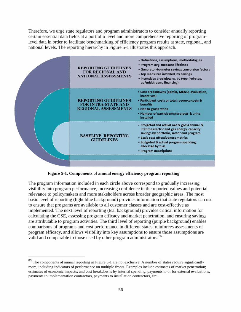
Therefore, we urge state regulators and program administrators to consider annually reporting certain essential data fields at a portfolio level and more comprehensive reporting of program-level data in order to facilitate benchmarking of efficiency program results at state, regional, and national levels. The reporting hierarchy in Figure 5-1 illustrates this approach.

Figure 5-1. Components of annual energy efficiency program reporting

The program information included in each circle above correspond to gradually increasing visibility into program performance, increasing confidence in the reported values and potential relevance to policymakers and more stakeholders across broader geographic areas. The most basic level of reporting (light blue background) provides information that state regulators can use to ensure that programs are available to all customer classes and are cost-effective as implemented. The next level of reporting (teal background) provides critical information for calculating the CSE, assessing program efficacy and market penetration, and ensuring savings are attributable to program activities. The third level of reporting (purple background) enables comparisons of programs and cost performance in different states, reinforces assessments of program efficacy, and allows visibility into key assumptions to ensure those assumptions are valid and comparable to those used by other program administrators.85

85 The components of annual reporting in Figure 5-1 are not exclusive. A number of states require significantly more, including indicators of performance on multiple fronts. Examples include estimates of market penetration; estimates of economic impacts; and cost breakdowns by internal spending, payments to or for external evaluations, payments to implementation contractors, payments to installation contractors, etc.

56

If program administrators were to report, at a minimum, the data under the baseline guidelines, this analysis would include nine additional program administrators among the 31 states included in this study, and programs from at least an additional 14 states. This would facilitate a more comprehensive national analysis of the impact of utility-customer funded energy efficiency. We also encourage program administrators, regulators and other stakeholders to provide feedback on our efforts to encourage consistent reporting of efficiency program results, particularly the program typology and data definitions. We will be soliciting input more formally as we move forward with the next phases of this project. Given sufficient interest and resources, it is our hope to update the LBNL DSM Program Impacts Database on a periodic basis and prepare comprehensive reports and policy briefs that are publicly available that explore key issues in energy efficiency programs.

57

6. References

ACEEE. 2013. State Energy Efficiency Resource Standards (EERS). Policy Brief. July. Accessed at: http://aceee.org/files/pdf/policy-brief/eers-07-2013.pdf.

Arimura, Toshi H., and Shanjun Li, Richard G. Newell, Karen Palmer. 2012. “Cost-Effectiveness of Electricity Energy Efficiency Programs.” The Energy Journal 33 (2).

Barbose, G. L., C.A. Goldman, I. M. Hoffman, M. A. Billingsley. 2013. The Future of Utility Customer-Funded Energy Efficiency Programs in the United States: Projected Spending and Savings to 2025. January. LBNL-5803E.

Consortium for Energy Efficiency (CEE). 2013. 2012 Industry Report. Found here: http://www.cee1.org/annual-industry-reports

Dixon, R.K., E. McGowan, G. Onysko, R.M. Scheer.US energy conservation and efficiency policies: Challenges and opportunities, Energy Policy, Volume 38, Issue 11, November 2010, Pages 6398-6408, ISSN 0301-4215, 10.1016/j.enpol.2010.01.038. http://www.sciencedirect.com/science/article/pii/S0301421510000637

Energy Information Administration. 2013. Levelized Cost of New Generation Resources in the Annual Energy Outlook 2013. Accessed at http://www.eia.gov/forecasts/aeo/er/electricity_generation.cfm.

Eto, Joseph, and Suzie Kito, Leslie Shown, Richard Sonnenblick. 2000. “Where Did the Money Go? The Cost and Performance of the Largest Commercial Sector DSM Programs.” The Energy Journal 21 (2): 23-49.

Friedrich, Katherine, and Maggie Eldridge, Dan York, Patti Witte, Marty Kushler. 2009. “Saving Energy Cost-Effectively: A National Review of the Cost of Energy Saved through Utility-Sector Energy Efficiency Programs.” American Council for an Energy-Efficient Economy Report Number U092, September.

Forster, H. J., Wallace, P., Dahlberg, N. 2013. “2012 State of the Efficiency Program Industry - Budgets, Expenditures, and Impacts” Consortium for Energy Efficiency. March. Accessed at: http://www.cee1.org/annual-industry-reports

Gillingham, Kenneth, and Richard Newell, Karen Palmer. 2006. “Energy Efficiency Policies: A Retrospective Examination.” Annual Review of Environment and Resources 31: 161-192.

Goldman, Charles A., Jane S. Peters, Nathaniel Albers, Elizabeth Stuart, and Merrian C. Fuller. Energy Efficiency Services Sector: Workforce Education and Training Needs. Berkeley: LBNL, 2010.

Hoffman, I.M., M.A. Billingsley, S.R. Schiller, C.A. Goldman, E. Stuart. 2013. “Energy Efficiency Program Typology and Data Metrics: Enabling Multi-State Analyses Through

58

http://aceee.org/files/pdf/policy-brief/eers-07-2013.pdf

http://www.cee1.org/annual-industry-reports

http://www.sciencedirect.com/science/article/pii/S0301421510000637

http://www.eia.gov/forecasts/aeo/er/electricity_generation.cfm

http://www.cee1.org/annual-industry-reports

the Use of Common Terminology.” Lawrence Berkeley National Laboratory Policy Brief. August.

Meier, A. K. 1984. The Cost of Conserved Energy as an Investment Statistic. Lawrence Berkeley National Laboratory. ESL-IE-84-04-109.

Meier, A. K. 1982. Supply Curves of Conserved Energy, Lawrence Berkeley National Laboratory, LBL-14686. May.

Molina, Maggie. 2014. “Still the First Fuel: National Review of Energy Efficiency Cost of Saved Energy.” American Council for an Energy-Efficient Economy (ACEEE). March.

Nadel, Steven, and Howard Geller. 1996. “Utility DSM - What have we learned? Where are we going?” Energy Policy 24 (4): 289-302.

National Action Plan for Energy Efficiency. 2008. Understanding Cost-Effectiveness of Energy Efficiency Programs: Best Practices, Technical Methods, and Emerging Issues for Policy- Makers. Energy and Environmental Economics, Inc. and Regulatory Assistance Project.

Northeast Energy Efficiency Partnerships (NEEP). 2011. Glossary of Terms. Regional Evaluation, Measurement and Verification Forum. July. Accessed at: http://neep.org/Assets/uploads/files/emv/emv-products/EMV_Glossary_Version_2.1.pdf.

Regional Energy Efficiency Database (REED). 2013. Accessed at: http://www.neep-reed.org/Disclaimer.aspx?Source=http://www.neep-reed.org/default.aspx.

SEE Action Network (State & Local Energy Efficiency Action Network). 2012. “Energy Efficiency Program Impact Evaluation Guide.” Prepared by Steven R. Schiller, Schiller Consulting, Inc. December. www.seeaction.energy.gov

U.S. Bureau of Labor Statistics. Income and Employment Report. July 2013

U.S. Energy Information Administration Form 861 survey data, 1999-2012

U.S. EIA Form 826 and 861 reports (the Monthly Electric Sales and Revenue Report with State Distributions Report and the Annual Electric Power Industry Report). August 2013.

59

http://neep.org/Assets/uploads/files/emv/emv-products/EMV_Glossary_Version_2.1.pdf

http://www.neep-reed.org/Disclaimer.aspx?Source=http://www.neep-reed.org/default.aspx

http://www.neep-reed.org/Disclaimer.aspx?Source=http://www.neep-reed.org/default.aspx