January 29, 2014 8:51 WSPC/S0218-1274 1450010

International Journal of Bifurcation and Chaos, Vol. 24, No. 1 (2014) 1450010 (11 pages)c© World Scientific Publishing CompanyDOI: 10.1142/S0218127414500102

Cost Function Based on Gaussian MixtureModel for Parameter Estimation of a Chaotic

Circuit with a Hidden Attractor

Seng-Kin Lao∗Department of Electromechanical Engineering,

University of Macau,Avenida Padre Tomas Pereira Taipa, Macau, P. R. China

skeltonl@umac.mo

Yasser ShekoftehBiomedical Engineering Department,Amirkabir University of Technology,

Tehran 15875-4413, IranResearch Center of Intelligent Signal Processing (RCISP)

Tehran, Irany shekofteh@aut.ac.ir

Sajad JafariBiomedical Engineering Department,Amirkabir University of Technology,

Tehran 15875-4413, Iransajadjafari@aut.ac.ir

Julien Clinton SprottDepartment of Physics, University of Wisconsin,

Madison, WI 53706, USAcsprott@wisc.edu

Received August 10, 2013

In this paper, we introduce a new chaotic system and its corresponding circuit. This systemhas a special property of having a hidden attractor. Systems with hidden attractors are newlyintroduced and barely investigated. Conventional methods for parameter estimation in modelsof these systems have some limitations caused by sensitivity to initial conditions. We use ageometry-based cost function to overcome those limitations by building a statistical model onthe distribution of the real system attractor in state space. This cost function is defined by theuse of a likelihood score in a Gaussian Mixture Model (GMM) which is fitted to the observedattractor generated by the real system in state space. Using that learned GMM, a similarityscore can be defined by the computed likelihood score of the model time series. The results showthe adequacy of the proposed cost function.

Keywords : Parameter estimation; chaotic circuits; Gaussian mixture model; cost function; statespace; stable equilibrium; hidden attractors.

∗Author for correspondence

1450010-1

Int.

J. B

ifur

catio

n C

haos

201

4.24

. Dow

nloa

ded

from

ww

w.w

orld

scie

ntif

ic.c

omby

CIT

Y U

NIV

ER

SIT

Y O

F H

ON

G K

ON

G o

n 02

/19/

14. F

or p

erso

nal u

se o

nly.

January 29, 2014 8:51 WSPC/S0218-1274 1450010

S.-K. Lao et al.

1. Introduction

Recently there has been increasing attention onsome unusual chaotic systems as those having noequilibrium, stable equilibria, or coexisting attrac-tors [Jafari et al., 2013b; Molaie et al., 2013;Uyaroglu & Pehlivan, 2010; Wang & Chen, 2012,2013; Wang et al., 2012a; Wang et al., 2012b;Wei, 2011a, 2011b; Wei & Yang, 2010, 2011, 2012].Recent research has involved categorizing periodicand chaotic attractors as either self-excited or hid-den [Bragin et al., 2011; Kiseleva et al., 2012;Kuznetsov et al., 2010; Kuznetsov et al., 2011a;Kuznetsov et al., 2011b; Kuznetsov et al., 2013;Leonov et al., 2010; Leonov et al., 2011a; Leonovet al., 2011b; Leonov et al., 2012; Leonov et al.,2013; Leonov & Kuznetsov, 2011a, 2011b; Leonov &Kuznetsov, 2012, 2013a, 2013b, 2013c]. A self-excited attractor has a basin of attraction that isassociated with an unstable equilibrium, whereas ahidden attractor has a basin of attraction that doesnot intersect with small neighborhoods of any equi-librium points. Thus any dissipative chaotic flowwith no equilibrium or with only stable equilibriamust have a hidden strange attractor. Only a fewsuch examples have been reported in the literature[Jafari et al., 2013b; Molaie et al., 2013; Uyaroglu &Pehlivan, 2010; Wang & Chen, 2012, 2013; Wanget al., 2012a; Wang et al., 2012b; Wei, 2011a, 2011b;Wei & Yang, 2010, 2011, 2012]. Hidden attractorsare important in engineering applications becausethey allow unexpected and potentially disastrousresponses to perturbations in a structure like abridge or an aeroplane wing. In this paper, we intro-duce a new chaotic system with a hidden attractorand its corresponding electronic circuit. Then weapply a new parameter estimation technique to thissystem.

A widely used method for parameter estimationof chaotic systems is optimization-based parameterestimation [Chang et al., 2008; Gao et al., 2009; Liet al., 2012; Li & Yin, 2012; Modares et al., 2010;Mukhopadhyay & Banerjee, 2012; Tang & Guan,2009; Tang et al., 2012; Tao et al., 2007; Tien &Li, 2012; Yuan & Yang, 2012]. In this method, theproblem of parameter estimation is formulated as acost function which should be minimized. Althoughthere are many optimization approaches availablefor this problem (e.g. genetic algorithm [Tao et al.,2007], particle swarm optimization [Gao et al.,2009; Modares et al., 2010], evolutionary program-ming [Chang et al., 2008]), they have one common

feature: they define a cost function based on simi-larity between the time series obtained from the realsystem and ones obtained from the model. They usetime correlation between two chaotic time series asthe similarity indicator. However, this indicator haslimitations. It is well known that chaotic systemsare sensitive to initial conditions [Hilborn, 2001].Thus there can be two completely identical (both instructure and parameters) chaotic systems that pro-duce time series with no correlation due to a smalldifference in initial conditions [Jafari et al., 2012;Jafari et al., 2013a]. One way to overcome this prob-lem is using near term correlation and to reinitializ-ing the system frequently (i.e. not letting significantdivergence of the trajectories occur). However, thisapproach also has limitations. In many systems, wedo not have access to a time series for all of the sys-tem variables, and thus the model cannot be reini-tialized. Hence, we prefer a new kind of similarityindicator and corresponding cost function.

Although chaotic systems have random-likebehavior in the time domain, they are ordered instate space and usually have a specific topologycalled a strange attractor. In this work, we proposea similarity indicator between these attractors as anobjective function for parameter estimation. To dothis, we model the attractor of the real system by astatistical and parametric model. In [Povinelli et al.,2004; Johnson et al., 2005; Shekofteh & Almasgani,2013b] a Gaussian Mixture Model (GMM) was pro-posed as a parametric model of a phoneme attractorin the state space. Their results of isolated phonemeclassification have shown that the GMM is a use-ful model to capture structure and topology of thephoneme attractors in the state space. Thus wepropose to use the GMM as a parametric modelof the strange attractor obtained from a real sys-tem. Based on the learned GMM, a similarity indi-cator can be achieved by matching the time seriesobtained from the model of a real system with dif-ferent sets of parameters to evaluate the propernessof each set. Therefore our proposed cost functionwill consist of two steps; first, a training stage whichincludes fitting a GMM to the attractor of the realsystem in the state space, and second, an evaluationstep to compute the similarity between the learnedGMM and the attractors of the model with esti-mated parameters.

The rest of the paper is organized as follows.Section 2 introduces the new chaotic model and itscorresponding electronic circuit. Section 3 details

1450010-2

Int.

J. B

ifur

catio

n C

haos

201

4.24

. Dow

nloa

ded

from

ww

w.w

orld

scie

ntif

ic.c

omby

CIT

Y U

NIV

ER

SIT

Y O

F H

ON

G K

ON

G o

n 02

/19/

14. F

or p

erso

nal u

se o

nly.

January 29, 2014 8:51 WSPC/S0218-1274 1450010

Cost Function Based on GMM for Parameter Estimation of a Chaotic Circuit

the proposed GMM-based cost function. In Sec. 4,our experimental results are introduced and dis-cussed. In Sec. 5 we show that using Takens’ theo-rem, this new method can be applied when we donot have access to all the time series from all thestate space variables. This is in fact the main benefitof the proposed method. Finally, we draw conclu-sions in the last section.

2. New Chaotic System andIts Corresponding Circuit

Consider the following chaotic system:

x = −z

y = −x − z

z = 2x − 1.3y − 2z + x2 + z2 − xz.

(1)

The parameters in this system have been set insuch a way that their values be deemed “elegant”[Sprott, 2010]. Typical initial conditions which arein the basin of attraction of strange attractor are(−0.1, 3.4,−1.7). There is only one equilibriumat the origin E(0, 0, 0), and it is stable. Thus apoint attractor coexists with the strange attractor.Figure 1 shows a cross-section in the xy-plane

Fig. 1. Cross-section of the basins of attraction of the twoattractors in the xy-plane at z = 0. Initial conditions in thewhite region lead to unbounded orbits, those in the red regionlead to the point attractor shown as a black dot, and thosein the light blue region lead to the strange attractor shownin cross-section as a pair of black lines.

at z = 0 of the basin of attraction for the twoattractors. Note that the cross-section of the strangeattractor nearly touches its basin boundary as istypical of low-dimensional chaotic flows. It is inter-esting that besides the area around the origin, thereis another separate area that converges to the stableequilibrium.

The eigenvalues that correspond to E(0, 0, 0)are

λ1 = −1.9783,

λ2 = −0.0108 + 0.8106i,

λ3 = −0.0108 − 0.8106i.

(2)

Since the characteristic equation has a negative realroot and two imaginary roots with negative realparts, E(0, 0, 0) is a stable focus. On the other hand,the Lyapunov spectrum for the strange attractorwas estimated as LE 1 = 0.018,LE 2 = 0,LE 3 =−2.018. Thus system (1) is believed to be chaoticand has only a single stable equilibrium, thoughpositive Lyapunov exponent is not always an indica-tion of chaos [Kuznetsov & Leonov, 2005; Leonov &Kuznetsov, 2007].

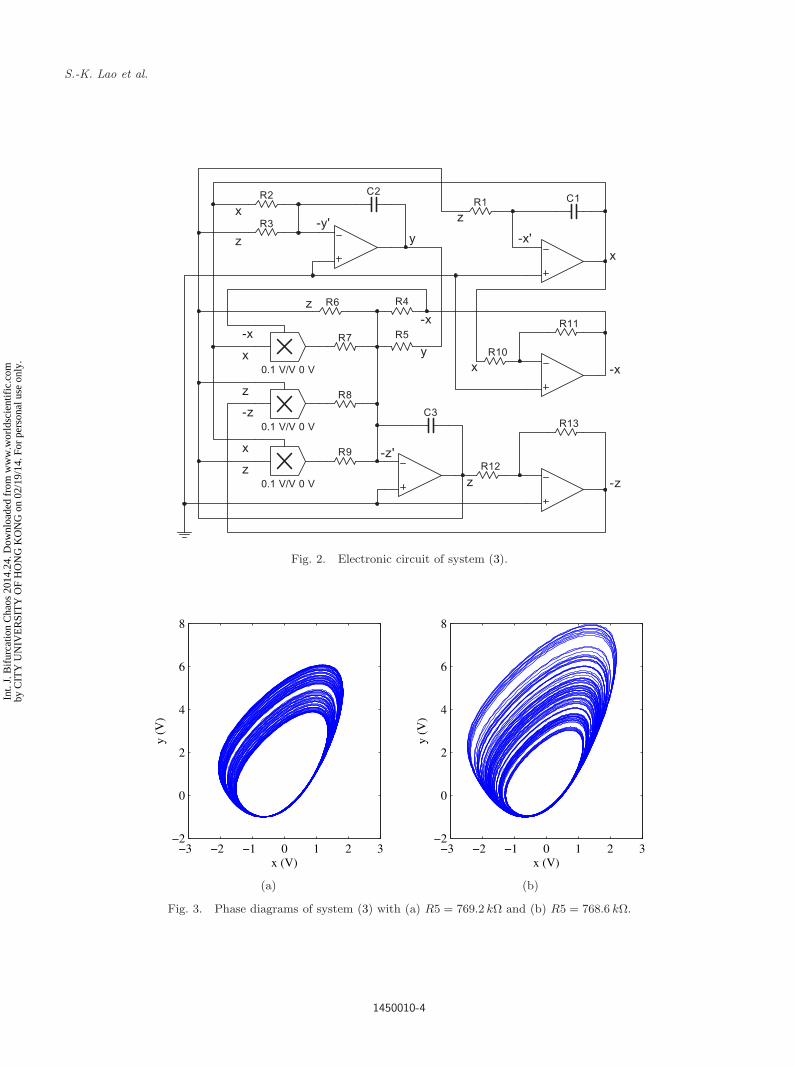
It is possible to produce electronic signals forthe above system. An electronic circuit, as shownin Fig. 2, was designed using operational amplifierssuch as summing amplifiers, inverting amplifiers,multipliers, and integrators. System (1) is rewrit-ten in the form of:

x = − 1R1C1

z

y = − 1R2C2

x − 1R3C2

z

z =1

R4C3x − 1

R5C3y − 1

R6C3z

+1

10R7C3x2 +

110R8C3

z2 − 110R9C3

xz.

(3)

The values of the resistors and capacitors are chosento be R1 = R2 = R3 = 1MΩ, R4 = 500 kΩ, R5 =769.2 kΩ, R6 = 500 kΩ, R7 = R8 = R9 = 100 kΩ,R10 = R11 = R12 = R13 = 1MΩ, and C1 = C2 =C3 = 1µF. The circuit was implemented in the elec-tronic simulation package MultisimR©. The initialcondition was selected as x0 = −0.1, y0 = 3.4, andz0 = −1.7. The phase diagram of system is plotted

1450010-3

Int.

J. B

ifur

catio

n C

haos

201

4.24

. Dow

nloa

ded

from

ww

w.w

orld

scie

ntif

ic.c

omby

CIT

Y U

NIV

ER

SIT

Y O

F H

ON

G K

ON

G o

n 02

/19/

14. F

or p

erso

nal u

se o

nly.

January 29, 2014 8:51 WSPC/S0218-1274 1450010

S.-K. Lao et al.

0.1 V/V 0 V

Y

X

R3

C2R2

R9

C3

R8

0.1 V/V 0 V

Y

X

0.1 V/V 0 V

Y

XR7

R6

R5

R4

R12

R13

y

z

-z

z

z

x

x

-x-x

y

-y'z

x

z

-z'

-z

R10

R11

x -x

R1 C1

x

z

-x'

Fig. 2. Electronic circuit of system (3).

−3 −2 −1 0 1 2 3−2

0

2

4

6

8

x (V)

y (V

)

−3 −2 −1 0 1 2 3−2

0

2

4

6

8

x (V)

y (V

)

(a) (b)

Fig. 3. Phase diagrams of system (3) with (a) R5 = 769.2 kΩ and (b) R5 = 768.6 kΩ.

1450010-4

Int.

J. B

ifur

catio

n C

haos

201

4.24

. Dow

nloa

ded

from

ww

w.w

orld

scie

ntif

ic.c

omby

CIT

Y U

NIV

ER

SIT

Y O

F H

ON

G K

ON

G o

n 02

/19/

14. F

or p

erso

nal u

se o

nly.

January 29, 2014 8:51 WSPC/S0218-1274 1450010

Cost Function Based on GMM for Parameter Estimation of a Chaotic Circuit

768.5 769 769.5 770 770.5 7712

4

6

8

y (V

)

R5 (kOhm)

Fig. 4. Bifurcation diagram of output yx=0 with varying R5in the electronic circuit.

in Fig. 3(a). In addition, a bifurcation diagram isplotted in Fig. 4 which is produced by varying R5.If we change R5 to 768.6 kΩ, a wider spread of thetrajectories of the system can be observed in thephase diagram depicted in Fig. 3(b). So it is veryimportant to estimate the parameters in an accu-rate way when modeling a chaotic system.

3. Proposed Cost FunctionBased on GMM

As mentioned before, the state space is a suitabledomain to represent chaotic and nonlinear behav-iors of a complex dynamical system. One of theadvantages of considering a signal in state spaceis its time-independent distribution. Based onthis characteristic, a statistical distribution of theobserved vectors in the state space can capture theattractor geometry and nonlinear system character-istics [Povinelli et al., 2004; Povinelli et al., 2006].The distribution of points on the attractor is invari-ant and independent of initial conditions providedthe initial conditions are in the basin of attractionand the time series is of infinite length [Kantz &Schreiber, 1997]. Thus we propose a similarity indi-cator using a conditional likelihood score betweena learned statistical model of a real system attrac-tor and a new distribution of an attractor obtainedby a specific model of the system. Here, we use aGMM as the statistical model. The GMM is a para-metric probability density function represented bya weighted sum of Gaussian component densities[Bishop, 2006]. GMMs were used as a parametricmodel of the probability distribution of state space

vectors in many different systems such as vocal-tract related features in speech recognition system[Shekofteh & Almasgani, 2013b; Jafari & Almas-ganj, 2012] or EGC signal classification methods[Nejadgholi et al., 2011; Roberts et al., 2001]. One ofthe powerful characteristics of the GMM is its abil-ity to form smooth approximations of attractors instate space [Nakagawa et al., 2012].

To find the similarity score between the attrac-tor of a real system and the state space points of themodel, we calculate likelihood scores which comefrom GMM computations. Our algorithm consistsof two steps; a training stage which includes fittingthe GMM to the attractor of the real system, andan evaluation stage to select the best set of param-eters in the model to optimize the similarity scorein the learned GMM. The following are the steps indetail.

Step 1. The first step of the proposed approach isthe learning phase. A GMM learns the probabilitydistribution of the attractor of the real system. Thismodel is a weighted sum of M individual Gaussiandensities. It can be represented by a set of systemparameters, λ, as follows,

λ =

wm, µm,∑m

, m = 1, . . . ,M

p(v |λ) =M∑

m=1

wm1

(2π)D/2

1∣∣∣∣∑m

∣∣∣∣1/2

× exp

−12

(v − µm)T−1∑m

(v − µm)

(4)

where M is the number of mixtures (Gaussian com-ponents), µm is the D-dimensional mean vector ofthe mth mixture,

∑m is the D × D covariance

matrix, and | · | denotes the determinant operator.Based on the observation vector v, in this work,D = 3 is selected. Also, p(v |λ) is the likelihood-based similarity score for the observed vector v.This score is obtained by giving v to the learnedGMM with its parameters of λ.

Using the prepared training data from theattractor of the real system, the parameters of theGMM are specialized to model the geometry ofthe attractor. As a popular and well-establishedmethod, maximum likelihood (ML) estimation is

1450010-5

Int.

J. B

ifur

catio

n C

haos

201

4.24

. Dow

nloa

ded

from

ww

w.w

orld

scie

ntif

ic.c

omby

CIT

Y U

NIV

ER

SIT

Y O

F H

ON

G K

ON

G o

n 02

/19/

14. F

or p

erso

nal u

se o

nly.

January 29, 2014 8:51 WSPC/S0218-1274 1450010

S.-K. Lao et al.

Fig. 5. GMM modeling (with M = 240 components) of the strange attractor for the introduced chaotic circuit in a 3-D statespace.

applied to identify the GMM parameters [Bishop,2006; Dempster et al., 1977]. However, there is noanalytical solution to determine the optimum num-ber of GMM mixtures needed for a specific problem,which depends on the complexity of the involveddata set [Jafari et al., 2010]. Figure 5 shows thestrange attractor of the new chaotic circuit in thethree-dimensional state space with its GMM mod-eling using 240 Gaussian component (M = 240),where every three-dimensional ellipsoid correspondsto one of the GMM’s Gaussian components.

Step 2. The second step of the proposed approachis finding the best model parameters using thelearned GMM in Step 1. Here, the search space willbe formed from a set of acceptable values of themodel parameters. Then, for each set of parame-ters (here a set of parameters k = a and b whichis described in Sec. 4), the model will be simu-lated, and a new attractor in the state space willbe obtained. Finally, the similarity score is com-puted using an average point-by-point likelihoodscore obtained from the learned GMM, λ, as follows:

p(V k |λ) =1N

N∑n=1

logp(vkn|λ) (5)

where V k is a matrix whose rows are composed fromthe state space vector of the model trajectory withthe model’s set of parameters k, and N is the num-ber of state space point in the V k matrix. The modelselection is accomplished by computing the condi-tional likelihoods of the signal under learned GMM

and selecting the parameters of a model that givesthe best similarity score.

Selection of the best set of parameters, k∗, usesthe following criteria. If we use the negative ofthe similarity score, then the parameter estimationbecomes a cost function minimization. Equation (6)shows the final cost function, J(k), based on thenegative of its mean log-likelihood score,

k∗ = arg minJ(k) and J(k) = −p(V k |λ) (6)

where k is the set of model parameters and λ isthe learned GMM of the real system attractor. Ourobjective is to determine the parameters of themodel, k, in such a way that J(k) is minimized.

4. Simulation Results

In this section, we do some simulations to investi-gate the acceptability of the proposed cost functionin estimating parameters of the chaotic circuit. Wehave used a fourth-order Runge–Kutta method witha step size of 10 ms and a total of 30 000 samplescorresponding to a time of 300 s.

Here, we consider a parametric model ofEq. (1):

x = −z

y = −x − z

z = 2x − 1.3y + az + x2 + bz2 − xz

(7)

where a and b are the parameters of the modelwhich should be estimated by minimization of the

1450010-6

Int.

J. B

ifur

catio

n C

haos

201

4.24

. Dow

nloa

ded

from

ww

w.w

orld

scie

ntif

ic.c

omby

CIT

Y U

NIV

ER

SIT

Y O

F H

ON

G K

ON

G o

n 02

/19/

14. F

or p

erso

nal u

se o

nly.

January 29, 2014 8:51 WSPC/S0218-1274 1450010

Cost Function Based on GMM for Parameter Estimation of a Chaotic Circuit

Fig. 6. The surface of the GMM-based cost function of J(k) for the introduced chaotic system of Eq. (7) along with avariation in their parameters, a and b.

(a) (b)

Fig. 7. Cross-section of the surface shown in Fig. 6 for (a) a = −2.00 and (b) b = 1.00.

proposed cost function. We used M = 240 mixturesto model the system attractor in state space.

If we plot the value of J(k), a cost “surface”can be obtained that shows dissimilarity betweenthe real system attractor and each model attrac-tor. In Fig. 6, such a surface is shown for the pro-posed cost function. The minimum on that surfacegives the parameters of the best model. In addition,Fig. 7 shows one-dimensional sections of the surface.The global minimum of the cost function is in theexpected place (a = −2.00 and b = 1.00). Moreover,the surface is almost convex, which makes it a sim-ple case for any optimization approach that movesdownhill.

5. Reconstruction of True DynamicsUsing Takens’ EmbeddingTheorem

One of the interesting topics in dynamical systemstheory is the embedding theorem introduced andused by Takens and Sauer [Kantz & Schreiber,1997]. It is also called the time-delay embeddingtheorem, and it gives the conditions under whicha chaotic system can be reconstructed from asequence of observations in a reconstructed phasespace (RPS). The RPS is a multidimensional spacewhose coordinates are produced by shift-delay sam-ples of a one-dimensional time series. The chaotic

1450010-7

Int.

J. B

ifur

catio

n C

haos

201

4.24

. Dow

nloa

ded

from

ww

w.w

orld

scie

ntif

ic.c

omby

CIT

Y U

NIV

ER

SIT

Y O

F H

ON

G K

ON

G o

n 02

/19/

14. F

or p

erso

nal u

se o

nly.

January 29, 2014 8:51 WSPC/S0218-1274 1450010

S.-K. Lao et al.

−4

−2

0

2

−5

0

5

10−2

−1.5

−1

−0.5

0

0.5

1

X(t)Y(t)

Z(t

)

−4

−2

0

2

−4

−2

0

2−3

−2

−1

0

1

2

X(t)X(t+ τ)

X(t

+2 τ

)

(a) (b)

Fig. 8. (a) A segment of the simulated time series in state space and (b) phase space reconstruction using only one variableof X(t) in the three-dimensional RPS (d = 3 and τ = 45).

and nonlinear behavior of such a signal is exhibitedin the RPS [Kantz & Schreiber, 1997; Shekofteh &Almasganj, 2013a; Kokkinos & Maragos, 2005]. Thesequence of embedded points of a signal in the RPSis commonly referred to as a signal trajectory. Toconstruct a signal trajectory, the samples must beembedded in the RPS. A single point of the embed-ded signal in the RPS is given by

Sl = [sl, sl+τ , sl+2τ , . . . , s(d−1)τ ] where

s = s1, s2, s3, . . . , sN (8)

where sl is the lth sample of an N -point segmentof the original one-dimensional signal s, d is theembedding dimension, and τ is the time lag. Theconcept of embedding dimension and time lag playsan important role in both practical and theoreticalaspects of the RPS [Povinelli et al., 2004; John-son et al., 2005; Shekofteh & Almasgani, 2013b;Kantz & Schreiber, 1997]. The minimum possibleembedding dimension can be identified by someheuristic procedures such as false nearest neigh-bor (FNN). Here, we use d = as a constant ofthe embedding dimension. Common techniques,including the first minimum of the auto-mutualinformation function or the first zero crossing of theauto-correlation function, have been used to iden-tify the preferred time lag of the RPS [Hilborn,2001; Kantz & Schreiber, 1997]. Here we selectτ = 45 which is calculated from the first minimumof the auto-mutual information function.

Figure 8 shows a segment of the simulated timeseries from Eq. (7) and its embedded trajectory inthe three-dimensional RPS (d = 3) only using onevariable of X(t). As can be seen in the figure, thereconstructed trajectory in the RPS has the samegeometric structure as the original simulated timeseries in state space.

Now, we do the same simulation as in Sec. 4to investigate the acceptability of the proposed costfunction in estimating parameters of the chaotic cir-cuit only using one variable. Here, we assume that

Cost Function

−2.005 −2.000 −1.995 −1.990 −1.985 −1.980

0.985

0.990

0.995

1.000

1.005

1.010

1.015

1.020−300

−250

−200

−150

−100

−50

0

b

a

Fig. 9. GMM-based cost function obtained from the recon-struction of X(t) in the RPS with a variation in the modelparameters of (7), a and b.

1450010-8

Int.

J. B

ifur

catio

n C

haos

201

4.24

. Dow

nloa

ded

from

ww

w.w

orld

scie

ntif

ic.c

omby

CIT

Y U

NIV

ER

SIT

Y O

F H

ON

G K

ON

G o

n 02

/19/

14. F

or p

erso

nal u

se o

nly.

January 29, 2014 8:51 WSPC/S0218-1274 1450010

Cost Function Based on GMM for Parameter Estimation of a Chaotic Circuit

0.98 0.99 1 1.01 1.02−50

0

50

100

150

200

250

300

b

Cos

t Fun

ctio

n

a = −2

−2.005 −2 −1.995 −1.99 −1.985 −1.98−50

0

50

100

150

200

250

300

a

Cos

t Fun

ctio

n

b = 1

(a) (b)

Fig. 10. Cross-sections of the cost function shown in Fig. 9 for (a) a = −2.00 and (b) b = 1.00.

the original chaotic system of (7) has the follow-ing real value of the parameters a = −2.00 andb = 1.00 which should be estimated by minimiza-tion of the proposed cost function. Similar to themethod proposed in Sec. 4, we use M = 240 mix-tures to model the attractor of the reconstructeddynamics of the variable X in the RPS. In Fig. 9,the calculated cost function J(k) is shown where theminimum point gives the parameters for the bestmodel. Moreover, Fig. 10 shows its one-dimensionalsections. As can be seen in these figures, the pro-posed cost function can give the true value of theglobal minimum (a = −2.00 and b = 1.00).

6. Conclusion

In this paper an appropriate and new cost functionhas been introduced to be used in parameter estima-tion of chaotic systems, based on a statistical modelof the real system attractor in state space. SinceGaussian Mixture Models (GMMs) are strong toolsto be used as parametric models of the probabilitydistribution of state space vectors in many differ-ent systems, we have used them in this work as thestatistical model. The proposed cost function is thenegative of a similarity metric which is formed byaveraging some log-likelihood scores. Overall resultsindicate that the global minimum of the proposedcost function is the true value of the model’s param-eters. Since this method is based on the topologyof strange attractors, one virtue is that the sampletime is not critical, and even with short and piece-wise time series, the GMM can be trained, althoughthe data do have to adequately cover the attractor.

This method has been applied to parameter esti-mation of chaotic circuits with hidden attractors.To do so, a new chaotic system has been proposedwhich has only one stable equilibrium and thus ahidden attractor. These kinds of systems are barelyinvestigated and are good cases for further studies.

References

Bishop, C. M. [2006] Pattern Recognition and MachineLearning (Springer).

Bragin, V. O., Vagaitsev, V. I., Kuznetsov, N. V. &Leonov, G. A. [2011] “Algorithms for finding hiddenoscillations in nonlinear systems,” J. Comput. Syst.Sci. Int. 50, 511–543.

Chang, J. F., Yang, Y. S., Liao, T. L. & Yan, J. J.[2008] “Parameter identification of chaotic systemsusing evolutionary programming approach,” ExpertSyst. Appl. 35, 2074–2079.

Dempster, A. P., Laird, N. M. & Rubin, D. B. [1977]“Maximum likelihood from incomplete data via theEM algorithm,” J. Roy. Stat. Soc. 39, 1–38.

Gao, F., Lee, J., Li, Z., Tong, H. & Lu, X. [2009] “Param-eter estimation for chaotic system with initial randomnoises by particle swarm optimization,” Chaos Solit.Fract. 42, 1286–1291.

Hilborn, R. C. [2001] Chaos and Nonlinear Dynamics :An Introduction for Scientists and Engineers (OxfordUniversity Press, UK).

Jafari, A., Almasganj, F. & Nabibidhendi, M. [2010]“Statistical modeling of speech Poincare sections incombination of frequency analysis to improve speechrecognition performance,” Chaos 20, 033106.

Jafari, A. & Almasganj, F. [2012] “Using nonlin-ear modeling of reconstructed phase space and fre-quency domain analysis to improve automatic speech

1450010-9

Int.

J. B

ifur

catio

n C

haos

201

4.24

. Dow

nloa

ded

from

ww

w.w

orld

scie

ntif

ic.c

omby

CIT

Y U

NIV

ER

SIT

Y O

F H

ON

G K

ON

G o

n 02

/19/

14. F

or p

erso

nal u

se o

nly.

January 29, 2014 8:51 WSPC/S0218-1274 1450010

S.-K. Lao et al.

recognition performance,” Int. J. Bifurcation andChaos 22, 1250053.

Jafari, S., Golpayegani, S. M. R. H., Jafari, A. H. &Gharibzadeh, S. [2012] “Some remarks on chaoticssystems,” Int. J. Gen. Syst. 41, 329–330.

Jafari, S., Golpayegani, S. M. R. H. & Darabad, M. R.[2013a] “Comment on ‘Parameter identification andsynchronization of fractional-order chaotic systems’,”[Commun. Nonlin. Sci. Numer. Simul. 17, 305–316],”Commun. Nonlin. Sci. Numer. Simul. 18, 811–814.

Jafari, S., Sprott, J. C. & Golpayegani, S. M. R. H.[2013b] “Elementary quadratic chaotic flows with noequilibria,” Phys. Lett. A 377, 699–702.

Johnson, M. T., Povinelli, R. J., Lindgren, A. C., Ye,J., Liu, X. & Indrebo, K. M. [2005] “Time-domainisolated phoneme classification using reconstructedphase spaces,” IEEE T. Speech Audio P. 13, 458–466.

Kantz, H. & Schreiber, T. [1997] Nonlinear Time SeriesAnalysis (Cambridge University Press, England).

Kiseleva, M. A., Kuznetsov, N. V., Leonov, G. A. &Neittaanmaki, P. [2012] “Drilling systems failures andhidden oscillations,” IEEE 4th Int. Conf. Nonlin. Sci.Complex, pp. 109–112.

Kokkinos, I. & Maragos, P. [2005] “Nonlinear speechanalysis using models for chaotic systems,” IEEE T.Speech Audio Process. 13, 1098–1109.

Kuznetsov, N. V. & Leonov G. A. [2005] “On stabilityby the first approximation for discrete systems,” 2005Int. Conf. Physics and Control, PhysCon 2005 2005,pp. 596–599.

Kuznetsov, N. V., Leonov, G. A. & Vagaitsev, V. I. [2010]“Analytical-numerical method for attractor localiza-tion of generalized Chua’s system,” IFAC Proc. 4,29–33.

Kuznetsov, N. V., Kuznetsova, O. A., Leonov, G. A. &Vagaitsev, V. I. [2011a] “Hidden attractor in Chua’scircuits,” Proc. 8th Int. Conf. Informatics in Control,Automation and Robotics, pp. 279–283.

Kuznetsov, N. V., Leonov, G. A. & Seledzhi, S. M.[2011b] “Hidden oscillations in nonlinear control sys-tems,” IFAC Proc. 18, 2506–2510.

Kuznetsov, N. V., Kuznetsova, O. A., Leonov, G. A. &Vagaitsev, V. I. [2013] “Analytical-numerical localiza-tion of hidden attractor in electrical Chua’s circuit,”Lecture Notes in Electrical Engineering 174, 149–158.

Leonov, G. A. & Kuznetsov, N. V. [2007] “Time-varyinglinearization and the Perron effects,” Int. J. Bifurca-tion and Chaos 17, 1079–1107.

Leonov, G. A., Vagaitsev, V. I. & Kuznetsov, N. V. [2010]“Algorithm for localizing Chua attractors based onthe harmonic linearization method,” Dokl. Math. 82,663–666.

Leonov, G. A. & Kuznetsov, N. V. [2011a] “Algorithmsfor searching for hidden oscillations in the Aizermanand Kalman problems,” Dokl. Math. 84, 475–481.

Leonov, G. A. & Kuznetsov, N. V. [2011b] “Analytical-numerical methods for investigation of hidden oscilla-tions in nonlinear control systems,” IFAC Proc. 18,2494–2505.

Leonov, G. A., Kuznetsov, N. V. & Vagaitsev, V. I.[2011a] “Localization of hidden Chua’s attractors,”Phys. Lett. A 375, 2230–2233.

Leonov, G. A., Kuznetsov, N. V., Kuznetsova, O. A.,Seledzhi, S. M. & Vagaitsev, V. I. [2011b] “Hid-den oscillations in dynamical systems,” Trans. Syst.Contr. 6, 54–67.

Leonov, G. A. & Kuznetsov, N. V. [2012] “IWCFTA2012Keynote Speech I — Hidden attractors in dynam-ical systems: From hidden oscillation in Hilbert–Kolmogorov, Aizerman and Kalman problems tohidden chaotic attractor in Chua circuits,” 2012 FifthInt. Workshop on Chaos-Fractals Theories and Appli-cations (IWCFTA), xv–xvii.

Leonov, G. A., Kuznetsov, N. V. & Vagaitsev, V. I. [2012]“Hidden attractor in smooth Chua systems,” PhysicaD 241, 1482–1486.

Leonov, G. A., Kiseleva, M. A., Kuznetsov, N. V. & Neit-taanmaki, P. [2013] “Hidden oscillations in drillingsystems: Torsional vibrations,” J. Appl. Nonlin. Dyn.2, 83–94.

Leonov, G. A. & Kuznetsov, N. V. [2013a] “Analytical-numerical methods for hidden attractors’ localization:The 16th Hilbert problem, Aizerman and Kalmanconjectures, and Chua circuits,” Numerical Methodsfor Differential Equations, Optimization, and Techno-logical Problems, Computational Methods in AppliedSciences, Vol. 27, pp. 41–64.

Leonov, G. A. & Kuznetsov, N. V. [2013b] “Hiddenattractors in dynamical systems: From hidden oscilla-tion in Hilbert-Kolmogorov, Aizerman and Kalmanproblems to hidden chaotic attractor in Chua cir-cuits,” Int. J. Bifurcation and Chaos 23, 1330002.

Leonov, G. A. & Kuznetsov, N. V. [2013c] “Predictionof hidden oscillations existence in nonlinear dynami-cal systems: Analytics and simulation,” Nostradamus2013 : Prediction, Modeling and Analysis of ComplexSystems, Advances in Intelligent Systems and Com-puting, Vol. 210, pp. 5–13.

Li, C., Zhou, J., Xiao, J. & Xiao, H. [2012] “Parame-ters identification of chaotic system by chaotic grav-itational search algorithm,” Chaos Solit. Fract. 45,539–547.

Li, X. & Yin, M. [2012] “Parameter estimation forchaotic systems using the cuckoo search algorithmwith an orthogonal learning method,” Chin. Phys. B21, 050507.

Modares, H., Alfi, A. & Fateh, M. [2010] “Parameteridentification of chaotic dynamic systems through animproved particle swarm optimization,” Expert Syst.Appl. 37, 3714–3720.

1450010-10

Int.

J. B

ifur

catio

n C

haos

201

4.24

. Dow

nloa

ded

from

ww

w.w

orld

scie

ntif

ic.c

omby

CIT

Y U

NIV

ER

SIT

Y O

F H

ON

G K

ON

G o

n 02

/19/

14. F

or p

erso

nal u

se o

nly.

January 29, 2014 8:51 WSPC/S0218-1274 1450010

Cost Function Based on GMM for Parameter Estimation of a Chaotic Circuit

Molaie, M., Jafari, S., Sprott, J. C. & Golpayegani,S. M. R. H. [2013] “Simple chaotic flows with onestable equilibrium,” Int. J. Bifurcation and Chaos(accepted).

Mukhopadhyay, S. & Banerjee, S. [2012] “Global opti-mization of an optical chaotic system by chaoticmulti-swarm particle swarm optimization,” ExpertSyst. Appl. 39, 917–924.

Nakagawa, S., Wang, L. & Ohtsuka, S. [2012] “Speakeridentification and verification by combining MFCCand phase information,” IEEE T. Audio Speech 20,1085–1095.

Nejadgholi, I., Moradi, M. H. & Abdolali, F. [2011]“Using phase space reconstruction for patient inde-pendent heartbeat classification in comparison withsome benchmark methods,” Comput. Biol. Med. 41,411–419.

Povinelli, R. J., Johnson, M. T., Lindgren, A. C. & Ye,J. [2004] “Time series classification using Gaussianmixture models of reconstructed phase spaces,” IEEET. Knowl. Data Eng. 16, 779–783.

Povinelli, R. J., Johnson, M. T., Lindgren, A. C.,Roberts, F. M. & Ye, J. [2006] “Statistical models ofreconstructed phase spaces for signal classification,”IEEE T. Sign. Process. 54, 2178–2186.

Roberts, F. M., Povinelli, R. J. & Ropella, K. M.[2001] “Identification of ECG arrhythmias using phasespace reconstruction,” Principles of Data Mining andKnowledge Discovery, Lecture Notes in Computer Sci-ence, Vol. 2168, pp. 411–423.

Shekofteh, Y. & Almasganj, F. [2013a] “Autoregres-sive modeling of speech trajectory transformed to thereconstructed phase space for ASR purposes,” Digit.Sign. Process. 23, 1923–1932.

Shekofteh, Y. & Almasgani, F. [2013b] “Feature extrac-tion based on speech attractors in the reconstructedphase space for automatic speech recognition sys-tems,” ETRI J. 35, 100–108.

Sprott, J. C. [2010] Elegant Chaos : Algebraically SimpleChaotic Flows (World Scientific, Singapore).

Tang, Y. & Guan, X. [2009] “Parameter estimation ofchaotic system with time-delay: A differential evolu-tion approach,” Chaos Solit. Fract. 42, 3132–3139.

Tang, Y., Zhang, X., Hua, C., Li, L. & Yang, Y.[2012] “Parameter identification of commensurate

fractional-order chaotic system via differential evolu-tion,” Phys. Lett. A 376, 457–464.

Tao, C., Zhang, Y. & Jiang, J. J. [2007] “Estimatingsystem parameters from chaotic time series with syn-chronization optimized by a genetic algorithm,” Phys.Rev. E 76, 016209.

Tien, J. & Li, T. S. [2012] “Hybrid Taguchi-chaos ofmultilevel immune and the artificial bee colony algo-rithm for parameter identification of chaotic systems,”Comput. Math. Appl. 64, 1108–1119.

Uyaroglu, Y. & Pehlivan, I. [2010] “Nonlinear Sprott94Case A chaotic equation: Synchronization and mask-ing communication applications,” Comput. Electr.Eng. 36, 1093–1100.

Wang, X. & Chen, G. [2012] “A chaotic system withonly one stable equilibrium,” Commun. Nonlin. Sci.Numer. Simul. 17, 1264–1272.

Wang, Z., Cang, S., Ochola, E. O. & Sun, Y.[2012a] “A hyperchaotic system without equilibrium,”Nonlin. Dyn. 69, 531–537.

Wang, X., Chen, J., Lu, J. A. & Chen, G. [2012b] “A sim-ple yet complex one-parameter family of generalizedLorenz-like systems,” Int. J. Bifurcation and Chaos22, 1250116.

Wang, X. & Chen, G. [2013] “Constructing a chaoticsystem with any number of equilibria,” Nonlin. Dyn.71, 429–436.

Wei, Z. & Yang, Q. [2010] “Anti-control of Hopf bifurca-tion in the new chaotic system with two stable node-foci,” Appl. Math. Comput. 217, 422–429.

Wei, Z. & Yang, Q. [2011] “Dynamical analysis of a newautonomous 3-D chaotic system only with stable equi-libria,” Nonlin. Anal. Real World Appl. 12, 106–118.

Wei, Z. [2011a] “Delayed feedback on the 3-D chaotic sys-tem only with two stable node-foci,” Comput. Math.Appl. 63, 728–738.

Wei, Z. [2011b] “Dynamical behaviors of a chaotic sys-tem with no equilibria,” Phys. Lett. A 376, 102–108.

Wei, Z. & Yang, Q. [2012] “Dynamical analysis of thegeneralized Sprott C system with only two stable equi-libria,” Nonlin. Dyn. 68, 543–554.

Yuan, L. & Yang, Q. [2012] “Parameter identificationand synchronization of fractional-order chaotic sys-tems,” Commun. Nonlin. Sci. Numer. Simul. 17, 305–316.

1450010-11

Int.

J. B

ifur

catio

n C

haos

201

4.24

. Dow

nloa

ded

from

ww

w.w

orld

scie

ntif

ic.c

omby

CIT

Y U

NIV

ER

SIT

Y O

F H

ON

G K

ON

G o

n 02

/19/

14. F

or p

erso

nal u

se o

nly.