cost-environment efficiency analysis of construction

1

Cost-environment efficiency analysis of construction industry in China: A materials

balance approach

Yujiao Xian a,b,c, Kexin Yang a,b, Ke Wang a,b,d,e,f,*, Yi-Ming Wei a,b,d,e, Zhimin Huang a,b,g

a Center for Energy and Environmental Policy Research, Beijing Institute of Technology, Beijing, China b School of Management and Economics, Beijing Institute of Technology, Beijing, China

c Productivity and Efficiency Measurement Laboratory, Department of Industrial and Systems Engineering, Texas

A&M University, College Station, Texas, USA d Sustainable Development Research Institute for Economy and Society of Beijing, Beijing, China

e Beijing Key Lab of Energy Economics and Environmental Management, Beijing, China f Department of Geographical Sciences, University of Maryland, College Park, Maryland, USA

g Robert B. Willumstad School of Business, Adelphi University, Garden City, NY, USA

Abstract: This study utilizes the data envelopment analysis technique with materials balance condition to

evaluate the inherent trade-offs between environmental and cost outcomes among different types of energy

consumptions in China’s construction industry. Environmental and cost efficiency that is decomposed into

technical efficiency and allocative efficiency are estimated, and the possible environmental impact and

economic cost of reallocating energy inputs for improving efficiency are obtained. The estimation results show

that: i) China’s construction industry has the ability to produce its current level of industrial added value with

fewer CO2 emissions and fewer energy input cost through removing technical inefficiency and adjusting energy

consumption structure. ii) There are 31.9% and 6.1% reduction potentials on CO2 emissions if this industry

attained the most environmentally efficient and the most costly efficient situation, respectively. iii) The average

shadow cost of CO2 emissions reduction in this industry is very low, suggesting that it should control CO2

emissions through optimizing energy consumption structure and improving energy efficiency, instead of relying

on end-of-pipe emission abatement technologies or emission trading systems.

Key words: CO2 emissions; cost efficiency; Data Envelopment Analysis; environmental efficiency; materials

balance condition; trade-offs

1 Introduction

Carbon dioxide (CO2) emissions derived from energy consumption make a major contribution to China’s

environmental problems associated with greenhouse gas emissions (Chen, Shen, Song, Shi and Li, 2017). As

one of the most carbon-intensive industries in China, the proportion of coal, oil, nature gas and electricity to the

energy consumption in construction industry during 2011-2015 are 11.3%, 73.1%, 0.4% and 14.8%, respectively.

The annual growth rate of energy consumption in China’s construction industry during 2011-2015, which

accounts for 34.8%, is higher than the annual growth rate of China’s total energy consumption (28.3%) and

* Corresponding author. Tel: 86-10-68918651. E-mail: [email protected], [email protected]

2

industrial energy consumption (23.5%). Moreover, the proportion of energy consumption in the construction

industry to the total energy consumption of the society also rises with almost 5% annual growth rate. Since 2010,

China’s new building construction has accounted for nearly half of the world’s new construction growth, but

the per capita building area in China is still far lower than other major developed countries (Zhou, Khanna, Feng,

Ke and Levine, 2018). The Report on Building Energy Consumption states that carbon emission reduction in

the construction industry is significant for meeting the peaking target of carbon emissions which would appear

no longer than 2030 (CABEE, 2017). Since CO2 emissions are the inevitable by-product of economic activities

with the environmental side effects, theoretically reasonable measurements of environmental and economic

(cost) efficiency of CO2 emissions are imperative for providing useful information on policy making for carbon

emission reduction and relative efficiency improvement (Wang and Wei, 2014; Halkos, Tzeremes and

Kourtzidis, 2016; Guo Zhang and Zhang, 2018; Zhang, Jin and Shen, 2018; Xian, Wang, Shi, Zhang, Wei and

Huang, 2018). It would lead to better trade-offs on environmental and economic outcomes of China’s

construction industry and the whole ecosystem.

A number of attempts have already been made to measure the economic and/or environmental efficiency

for construction industry. For instance, Tatari and Kucukvar (2011) proposed an analytical tool to measure the

eco-efficiency of construction materials by using Data Envelopment Analysis (DEA) and a linear programming-

based mathematical approach. Xue, Wu, Zhang, Dai and Su. (2015) pointed out that DEA-based Malmquist

productivity index is a proper way to evaluate the energy consumption efficiency, and measured the change on

energy consumption productivity for China’s construction industry from 2004 to 2009 among 26 provinces.

Chancellor and Lu (2016) estimated construction productivity and efficiency in China from 1995 to 2012, and

pointed out that construction productivity has experienced a significant growth since 1995. Zhang, Li, Xia and

Skitmore (2018) used a modified DEA method to analyze the carbon efficiency which was decomposed into

several carbon efficiencies of different building materials such as cement, steel, and aluminum. The results

showed that in most China’s provinces, the carbon efficiencies are quite low, particularly for aluminum related

carbon emissions.

The studies mentioned above are limited in improving technical or environmental efficiency on the trade-

offs of economic outcomes and environmental emissions, and ignored to consider the allocative efficiency

through adjusting inputs. Hence, they might obtain limited economic meanings and policy implications for

China’s construction industry. Indeed, there are some efficiency evaluation had been decomposed into technical

efficiency and allocative efficiency (Shi and Grafton, 2010; Shi, 2010; Wang, Wei and Huang, 2018; Wang,

Yang, Wei and Zhang, 2018). However, they only distinguish the allocation between pollution related inputs

(e.g., energy) and non-pollution related inputs, but not focus on the allocation among different pollution-related

inputs (e.g., fossil fuels and renewables).

The pollution-generating technologies in efficiency evaluation can be generally formalized in five ways: i)

treating pollution as free disposable inputs (Reinhard, Knox Lovell and Thijssen, 2000; Mahlnerg and Sahoo,

2011). ii) considering pollutions as outputs under the weak disposability assumption (Färe, Grosskopf and

3

Tyteca, 1996; Fahlen and Ahlgren, 2012; Kwon, Cho and Sohn, 2017; Zhang, Sun and Huang, 2018). iii) using

the sum of the additive/multiplicative inverse of pollution values as outputs values (Seiford and Zhu, 2002;

Wang et al., 2012). iv) treating pollutions as costly disposable outputs in the by-production model (Førsund,

2009; Murty, Russel and Levkoff, 2012; Xian, Wang, Wei and Huang, 2019). However, these ways all have a

disadvantage of violating the first law of thermodynamics, and thus, might obtain the biased estimation results

of efficiency evaluation, especially when concerning the physical productivity and needing to quantify energy

flows through industrial systems. (Hampf and Rødseth, 2015; Wang, Mi and Wei, 2018). The influence of

construction activities (e.g., demolition of buildings) on the environmental system, the utilization of natural

resources (e.g., coal and oil), and the problems of cutting down emissions (e.g., CO2 emissions) all should be

considered into efficiency evaluation of the construction industry when including the emissions from energy

consumption. Hence, it is vital of important to quantify the energy or materials flows through construction

activities.

Based on the law of thermodynamics and materials balance principle (MBP) condition, this study assumes

the inevitability of generating residuals. We propose four data envelopment analysis based (DEA-based) models

with MBP to estimate technical efficiency (TE), environmental efficiency (EE), cost efficiency (CE), and total

cost efficiency (TCE) in China’s construction industry, respectively. In addition, the environmental and cost

trade-offs could also be identified in this industry.

This study’s primary contribution is that it provides a method that can help policy makers and managers to

balance the economic costs and ecological benefits of carbon abatement in the construction industry. In addition,

because of the predominate role of fossil-fuel in carbon discharges for China’s construction industry, this method

also provides an assessment on the allocation efficiency of energy inputs, and the costs and benefits of

substituting one fuel with another.

This paper is organized as follows: Section 2 introduces the materials balance principle, and Section 3

presents the DEA-based models for environmental and cost efficiency measurement with MBP. In section 4, we

describe the datasets and their resources. Section 5 presents the estimation results and discussions. Section 6

draws the conclusions.

2 Materials balance principle

Materials balance principle (MBP) is the balance of the materials between inputs, desirable outputs and

undesirable outputs in the production progress. Ayres and Kneese (1969) first introduced the materials balance

principle from the theoretical perspective, and then Lauwers, Van Huylenbroeck and Rogiers (1999) introduced

it in the use of efficiency and productivity measurement. Furthermore, Colli, Lauwers and Van Huylenbroeck

(2005) and Colli Lauwers and Van Huylenbroeck (2007) presented the aspects of the MBP in the DEA

technique, and concluded that the DEA-based MBP method is more tightly linked to the economic analysis

when measuring the efficiency and productivity than other DEA-based methods. The MBP method, which can

4

all concern the physical efficiency, economic prices and pollution cost, closely ties the production efficiency

and productivity with environmental and economic context. It bridges the gap between conventionally

environmental efficiency and economic efficiency, and thus, makes the environmental and economic outcomes

equally explicit.

MBP declares that the total amount of emission contents (i.e., carbon) in the inputs must equal the emission

contents in desirable output plus the emission contents in the residuals that may cause CO2 emissions. In specific,

the balance equation can be written as:

x y u a (1)

where x, y, u denotes the inputs, desirable outputs and undesirable outputs, respectively. a denotes the abatement

amount of pollutants. a=0 represents the situation in which there is no carbon abatement activities, and a>0

represents the situation in which the carbon abatement activities are implemented. In addition, and are

the vectors of emission factors in inputs and the vectors of recuperation factors in desirable outputs, respectively.

0 if x is non-polluting input, whereas 0 if x is polluting input. Similarly, 0 if desirable output y

does not contain polluting mass (i.e., carbon), whereas 0 if desirable output y contains polluting mass.

The MBP satisfies the weak G-disposability assumption (i.e., the laws of thermodynamics) that is a

summing-up formulation (Welch and Barnum, 2009). This assumption states that the increase in pollution (i.e.,

Δu) should equals the sum of three components: the increase in emission bound in input (i.e., αΔx), the reduction

in emission bound in desirable output (i.e., βΔy ), and the reduction in abatement of pollution (i.e.,Δa). Moreover,

the weak G-disposability formulation can be written as:

u x y a (2)

3 Efficiency measurement

In this sub-section, following Wang, Mi and Wei (2018), we propose four DEA-based MBP models to

estimate technical efficiency (TE), environmental efficiency (EE), cost efficiency (CE) and total cost efficiency

(TCE) for adjusting polluting inputs and associated pollutions, respectively.

This study considers a sample with n observations, and each observation j has polluting (i.e., energy) inputs,

non-polluting (non-energy) inputs, desirable outputs and undesirable outputs (i.e., pollutions or emissions)

denoted by ( , )E NE

ij mj rj ijx ,x y ,u , where i=1,…,l, m=1,…,f, r=1,…,s, and j=1,…,n.

First, for technical efficiency, in the situation that the observed inputs are not located on the efficient

boundary of the technology set, it can be projected onto the efficient boundary of the technology set by

proportionally shrinking the observed inputs. That is, by solving the following DEA-based minimizing

programming with MBP for the under estimated observation j0:

5

0

0

0

0

1

1

1

1

1, ,

1, ,

1, ,

1, ,

1, , 1

,

,

,

,

,

E

NE

E

T

nT E E Tx

ij j ij ijj

nNE NE Tx

mj j mj mjj

nTy

rj j rj rjj

nT Tu

ij j ij ijj

Tx Tu

ijij ij

min

s.t. x x d

x x d m

y y d r

u u d

d d j

i l

f

s

i l

i l

, ,n

(3)

where ETx

ijd , NETx

mjd , Ty

rjd and Tu

ijd respectively represents the slack variables of polluting input, non-polluting

input, desirable output and pollution implementing the weak G-disposability of MBP; j represents the

intensity variables indicating the convex combination of all observations; and ij is the emission factor

denoting the unit emission bound in polluting input. In addition, objective function T , which represents the

TE, would proportionally shrink all observed polluting inputs until they are projected onto the efficient boundary

of the technology set. The last equation associated with the first and four equations is the MBP condition.

Second, for environmental efficiency, since the amount of desirable output yr (r=1,…,s) is fixed, the

emission content x y will be minimized when the emission content in inputs (i.e., x ) is minimized.

Thus, the objective of EE is to achieve the minimal amount of emission content in all polluting inputs. Given

the desirable output yr (r=1,…,s), the associated DEA-based minimizing programming with MBP for the under

estimated observation j0 can be written as follows:

0 0

0

0

0

0

1

1

1

1

1

1, ,,

,

,

1, ,

1, ,

,, 1,

E

NE

E

lE E

i iji

nE E E Ex

i ij j ij ijj

nNE NE Ex

mj j mj mjj

nEy

rj j rj rjj

nE Eu

i ij j ij i

i

jj

i

x

j

j

E

ij

min x

s.t. x x d

x x d m

y y d r

u

i l

f

s

i l

u d

d d

1, , 1, ,,Eu

ij i l j n

(4)

Similarly, in model (4), EEx

ijd , NEEx

mjd , Ey

rjd and Eu

ijd respectively represents the slack variables of polluting

input, non-polluting input, desirable output and pollution implementing the weak G-disposability of MBP; j

6

represents the intensity variables; ij is the emission factor; and the last equation associated with the first and

four equations indicates the MBP condition. Moreover, E

i represents the variable for adjusting each polluting

input and its associated undesirable output, and the adjustment can be different among different polluting inputs

and undesirable outputs. It measures the resource allocation efficiency of each polluting input and the trade-offs

among different types of these inputs.

After solving model (4), the EE, which is the ratio of minimal emission content over observed emission

content, can be estimated by:

1

1

,, 1 ,

El

E E Ex

i ij iji

lE

i ji

ij

ij

n.

x d

EE j

x

(5)

The value of EE takes between zero and one, and EE=1 indicates that there is no possible to generate the

observed amount of desirable output with a smaller emission using the currently available technology.

Furthermore, EE can be decomposed into environmentally allocative efficiency (EAE) and environmentally

technical efficiency (ETE) as follows:

1

1

1 1

1 1

1, ,

E

E E

E

lE E Ex

i ij iji

lE

iji

l lE E Ex T E Tx

i ij ij ij iji i

l lT E Tx E

ij ij ij

ij

ij

ij ij

ij iji i

x d

EE

x

x d x d

x d x

EAE ETE, j

n.

(6)

where EAE relates to the correct polluting input mix, and ETE relates to the operation on the efficient production

frontier. The value of EAE and ETE both take between zero and one, and the one value indicates full efficiency.

Third, for cost efficiency, if the prices of polluting inputs are all available, the objective of CE is to obtain

the minimal amount of cost on all polluting inputs. Hence, the associated DEA-based minimizing programming

with MBP for the under estimated observation j0 can be written as follows:

7

0 0

0

0

0

0

1

1

1

1

1

1, ,,

,

,

1, ,

1, ,

,, 1,

E

NE

E

lC E

i iji

nC E E Cx

i ij j ij ijj

nNE NE Cx

mj j mj mjj

nCy

rj j rj rjj

nC Cu

i ij j ij i

i

jj

i

x

j

j

C

ij

min x

s.t. x x d

x x d m

y y d r

u

p

i l

f

s

i l

u

d

d d

1, , 1, ,,Cu

ij i l j n

(7)

whereECx

ijd , NECx

mjd , Cy

rjd and Cu

ijd respectively represents the slack variables of polluting input, non-polluting

input, desirable output and pollution implementing the weak G-disposability of MBP; 0ijp is the price of

polluting input; and the last equation indicates the MBP condition. Similar with model (4), C

i is the variable

for adjusting each polluting input and its associated undesirable output to achieve the minimal cost. It measures

the cost allocation efficiency of each polluting input, and measures the trade-offs among different types of these

inputs.

Replacing the emission factors in equation (5) and (6), CE and its two components of costly allocative

efficiency (CAE) and costly technical efficiency (CTE) can be computed as:

1

1

1 1

1 1

1, ,

E

E E

E

ij

ij

ij ij

lC E Cx

i ij iji

lE

iji

l lC E Cx T E Tx

i ij ij ij iji i

l lT E Tx E

ijij ijij iji i

x d

CE

x

x d x d

x d x

CAE CTE, j

p

p

p p

p p

n.

(8)

For each j (j=1,…,n) observation, except for the values associated with minimal emission

* *

1

El

E E Ex

i ij ijiji

x d and minimal cost * *

1

El

C E Cx

i ij ijiji

p x d , two additional values can be identified:

(i) the cost relating to the emission minimizing point, * *

1

El

E E Ex

i ij ijiji

p x d ; and (ii) the emission relating

to the cost minimizing point, * *

1

El

C E Cx

i ij ijiji

x d . *E

i , *EEx

ijd , *C

i , *ECx

ijd are the optimal solutions

of model (4) and (7). Hence, the cost of moving from the cost minimizing point to the emission minimizing

8

point can be identified as * * * *

1 1

E El

ij ij

lE E Ex C E Cx

i ij ij i ij iji i

p x d x d p . This cost could be named as the

shadow cost (SC) of emission reduction. In addition, the emission surplus consequences of shift from the

emission minimizing point to the cost minimizing point can be similarly identified as

* * * *

1 1

E El

ij ij

lC E Cx E E Ex

i ij ij i ij iji i

x d x d . This difference could be named as shadow emission (SE)

of cost reduction.

Finally, for total cost efficiency, the cost of polluting inputs and the cost of pollutions are both taken into

consideration. Then, a new minimal cost would be identified. The sum of the economic cost of polluting input

and the social cost of pollutions is interrupted as total cost. In this case, the associated DEA-based minimizing

programming with MBP for the under estimated observation j0 can be written as follows:

0 0 0

0

0

0

0

1

1

1

1

1

,

,

1, ,

1, ,

1,

1 ,,

,

,

,

E

NE

lTC E

i iji

nTC E E TCx

i ij j ij ijj

nNE NE TCx

mj j m

ij

j mjj

nTCy

rj j rj rjj

nTC TCu

i ij j ij i

ij

jj

ijmin x

s.t. x x d

x x d m

y y d r

p w

i l

f

s

iu u d

l

1, , 1,, ,ETCx TC

i

u

ijj ij i l nd d j

(9)

In model (9), 0ijw is the price of polluting input;

ETCx

ijd , NETCx

mjd , TCy

rjd and TCu

ijd respectively represents the

slack variables of polluting input, non-polluting input, desirable output and pollution; and the last equation

indicates the MBP condition. TC

i is the variable for adjusting each polluting input and its associated undesirable

output to achieve the totally minimal cost.

Then, TCE and its two components of total cost allocative efficiency (TCAE) and total cost technical

efficiency (TCTE) can be formulated as:

9

0 0

0 0

0 0 0 0

0 0 0 0

1

1

1 1

1 1

E

E E

E

lTC E TCx

i ij iji

lE

iji

l lTC E TCx

ij ij ij

ij ij ij

ij ij ij ij ij

T

ij

ij ij ij ij ij

E Tx

i ij ij ij iji i

l lT E Tx E

ij iji

ij iji

x d

TCE

x

x d x

p

d

w

p w

p

x d x

w p w

T

p p w

CAE

w

1, ,TCTE, j n.

(10)

The estimation of TCE could help to assess the impact of carbon price (e.g., allowance price and carbon

taxes) on the environmental efficiency and the amount of CO2 emissions.

4 Dataset and descriptive statistics

This research contains the data of China’s 27 provincial construction industry sectors during the period of

2011-2015. Heilongjiang, Guangxi, and Hainan are not included because they do not have coal consumption

data in their construction industries.

Our study focuses on the inherent trade-offs between environmental and cost outcomes among different

types of energy consumptions in China’s construction industry. The CO2 emissions is considered as the

environmental outcome, and the added value of construction industry is considered as the economic outcome.

We use different kinds of CO2 emissions from the consumption of coal, oil, and electricity in either the

construction phase of buildings or the construction activities. Moreover, the other inputs data for the construction

industry are also be taken into consideration. We use seven non-energy inputs: the net value of fixed asset, labor,

and construction materials including cement, steel, glass, wood, and aluminum; three energy inputs: coal, oil,

and electricity. Additionally, the provincial CO2 emission factors and the prices of coal, oil, and electricity are

considered in our calculation.

The data of energy consumptions (i.e., coal consumption, oil consumption, and electricity consumption)

are obtained from the energy balance table (the subsector of “construction” within the “total final consumption”

sector) in the China Energy Statistical Yearbook, whereas the construction materials data are collected from the

China Statistical Yearbook on Construction. The data of added value of construction industry, the net value of

fixed asset, and labor are collected from the China Statistical Yearbook. For CO2 emissions, we first calculate

the CO2 emissions from the combustion of coal and oil through referring the CO2 emission factors (IPCC,

2006) and the calorific values (NRDC, 2008). As for the CO2 emissions of electricity, we first obtain the CO2

emissions of the national electricity generation according to the associated primary energy consumption in

electricity generation, and then we use the ratio of the amount of electricity consumption for the construction

industry by the national electricity consumption to calculate the CO2 emissions from electricity in the

construction industry. Furthermore, the CO2 emission factors of each energy input for each province, which is

10

named as provincial CO2 emission factors of each energy input, are the ratio of the amount of CO2 emissions of

an energy to the amount of the associated energy consumption. Because of the different energy consumption

structure among provinces, the provincial CO2 emission factors are also various among provinces. The

information on prices of all energy are derived from Wind Data and the database of China National Coal

Association. The price of CO2 emissions is the seven pilot carbon markets’ average price of CO2 emission

allowance during 2013-2016 (i.e., 33.39 Yuan/tonne) which is obtained from the China’s carbon trading website.

We first obtain the average price of CO2 emissions in each pilot carbon market during 2013-2016, and then we

use the arithmetic average price of CO2 emissions for these seven pilots as the national price of CO2 emissions.

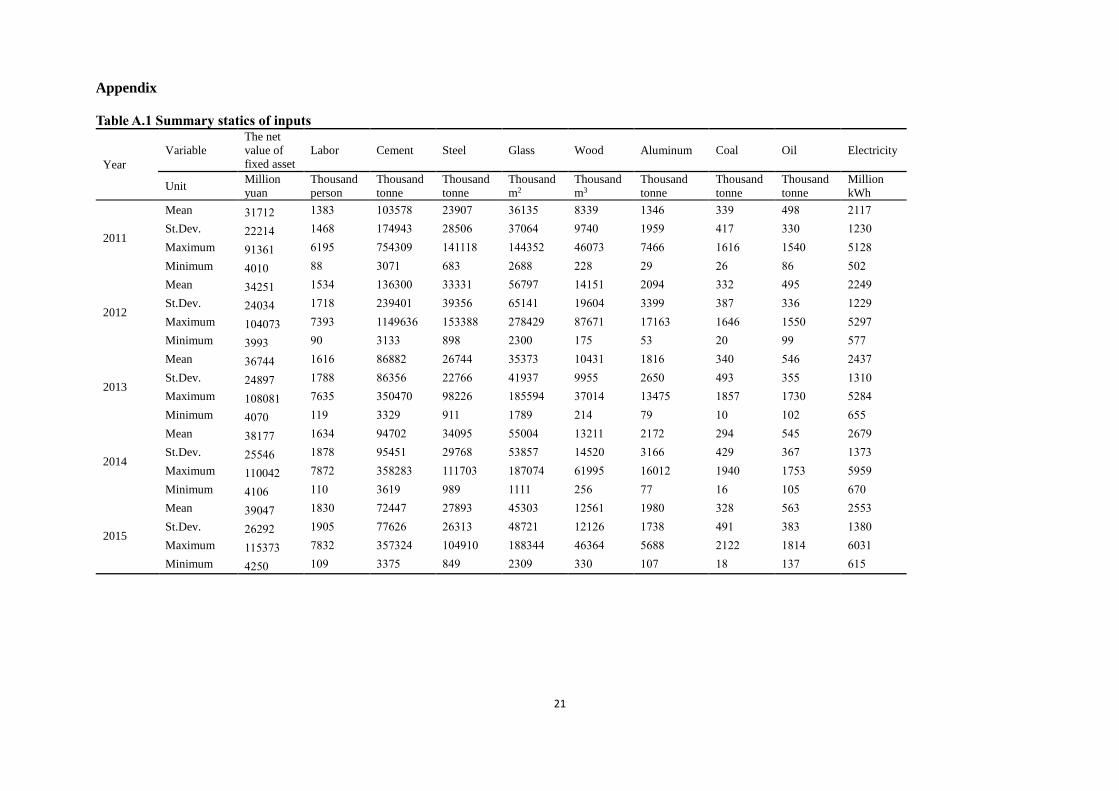
Tables 1 to 4 presented in the Appendix describe the summary statistics of the input and output data, provincial

CO2 emission factors, and prices of energy inputs.

5 Results and discussions

5.1 Environmental and cost efficiency

The efficiency measurement results of EE, CE and TCE are presented in Table 1 and Fig. 1. It is worth

noting that the mean value, maximum value and minimum value of CE and TCE, and their components, are

very close. The reason is that the pollution price is quite small compared with the price of polluting inputs. It

leads that the total cost is also quite close to the cost of polluting inputs. Therefore, the results of CE and TCE

are similar, and we will focus on TCE and its corresponding results in the following discussions.

On the one hand, for environmental efficiency, the mean value of 0.678 implies that China’s construction

industry on average could be able to produce its currently industrial added value with 32.2% fewer CO2

emissions associated with polluting inputs during 2011-2015. In addition, the mean values of EAE (0.707) and

ETE (0.943) indicate that the average sector of construction industry has the ability to produce its currently

industrial added value with 29.3% fewer carbon emissions from polluting input through energy consumption

structure optimization and with 5.7% fewer carbon emissions from polluting input through technical efficiency

improvement of energy consumption. On the other hand, for total cost efficiency, its mean value (0.663) suggests

that the construction industry could be able to reduce 33.7% total cost on average maintaining its current amount

of industrial added value. In specific, the average sector of construction industry could reduce 8.6% total cost

through removing technical inefficiency and reduce 29.5% total cost through adjusting energy consumption

structure during 2011-2015.

Table 1 Efficiency measurement results

EE EAE ETE CE CAE CTE TCE TCAE TCTE

Mean 0.678 0.707 0.943 0.662 0.705 0.913 0.663 0.705 0.914

St. Dev. 0.348 0.342 0.084 0.359 0.344 0.125 0.359 0.344 0.123

Maximum 1 1 1 1 1 1 1 1 1

Minimum 0.072 0.076 0.652 0.056 0.061 0.426 0.056 0.062 0.433

11

Figure 1 Box plot of different efficiency and their decomposition

Associated with the efficiency changes, total values on energy savings and CO2 emission reductions of the

27 provincial construction industry sectors are identified and reported in Table 2. The changes on polluting

inputs and total CO2 emissions are all annual average values. Firstly, Table 2 shows that China’s construction

industry would annually reduce 3.2 million tonnes of coal consumption (36.4%), 4.1 million tonnes of oil

consumption (28.8%) and 15.6 billion kWh of electricity consumption (24.0%) to produce the same industrial

added value if the technical inefficiency was eliminated in this industry. Then, the total CO2 emissions would

reduce by 28.7% (30.0 million tonnes).

Table 2 Changes on polluting inputs and CO2 emissions associated with efficiency changes

Polluting inputs and CO2 Unit Change

Absolute value Percentage (%)

Observation to TE

Coal Million tonne -3.2 -36.4

Oil Million tonne -4.1 -28.8

Electricity Billion kWh -15.6 -24.0

Total CO2 emissions Million tonne -30.0 -28.7

Observation to EE





Observation to TCE





TCE to EE

Coal Thousand tonne -196.6 -3.5

Oil Thousand tonne 163.0 1.8

Electricity Million kWh -655.6 -1.3

12

Total CO2 emissions Thousand tonne -389.3 -0.5

Secondly, if the construction industry was environmentally efficient, it would annual decrease 3.4 million

tonnes of coal consumption, 5.0 million tonnes of oil consumption and 15.8 billion kWh of electricity

consumption keeping its current industrial added value unchanged. Correspondingly, the construction industry

would annually decrease its total CO2 emissions by 31.9% (33.3 million tonnes). Specifically, to realize this

reduction of CO2 emissions, this industry needs to reduce its coal consumption by 38.6%, oil consumption by

34.6%, and electricity consumption 24.4%.

Thirdly, it can be notable that there is 36.4% (3.02 million tonnes), 35.8% (5.1 million tonnes) and 23.4%

(15.2 billion kWh) reduction potentials on coal consumption, oil consumption and electricity consumption if

China’s construction industry is costly efficient. Moreover, the total CO2 emissions would reduce by 6.3 million

tonnes (6.1%). This indicates that the achievement of cost minimizing for energy input mix would be helpful to

save all types of energy consumption and to control their corresponding CO2 emissions in China’s construction

industry.

Finally, it can be seen that there is 196.6 thousand tonnes and 655.6 million kWh reduction potentials on

coal and electricity consumption, associated with an increase of 163 thousand tonnes of oil consumption, if the

average industry removing from the cost minimizing point to emission minimizing point. Correspondingly, the

construction industry would have annually average 389.3 thousand tonnes (0.5%) reduction potentials on total

CO2 emissions through adjusting energy consumption structure, that is, reducing coal consumption and

electricity consumption by 3.5% and 1.3%, and increasing oil consumption by 1.8% as a compensation. This is

a powerful implication that the optimization of energy consumption structure is an efficient way to control

carbon emissions in China’s construction industry with reasonable amount of cost increase.

5.2 Environmental and cost trade-offs

The estimation results of environmental and cost trade-offs in emission are illustrated in Tables 3 and 4. At

the national average level, the construction industry would decrease CO2 emissions of per unit industrial added

value of construction sector by 29.3% if it was on the technically efficient frontier, and by 32.2% if it was

environmentally efficient. Simultaneously, this industry would averagely decrease total cost of per unit

industrial added value by 29.5% if it was technically efficient, and by 33.7% if it was on the costly efficient

frontier. These 29.3% and 29.5% decreases imply that if the construction industry could remove the technical

inefficiency, its generation cost and CO2 emissions would both reduce by more than one quarter. Therefore, in

the short term, there is no need to purchase expensive technologies on carbon control in China’s construction

industry, such as carbon capture and storage technology, for CO2 emission reduction.

In addition, Table 3 shows that the construction industry would have 31.7% reduction potentials on CO2

emissions of per unit industrial added value if it was costly efficient, and would have 4.9% more reduction

potentials on CO2 emissions of per unit industrial added value if it continued shifting to the totally cost

13

minimizing point along the technical efficiency frontier. These reduction percentages suggest that the

construction industry would reduce CO2 emissions by achieving the costly efficient point, i.e., cost efficiency

promotion would not lead to extra CO2 emissions on cost reduction. Table 4 presents that the average industry

would decrease 33.2% total cost of per unit industrial added value if having attained cost efficiency, and would

decrease 7.7% more total cost of per unit industrial added value if it continued reaching the emission minimizing

point along the technical efficiency frontier. These results indicate that approaching the environmentally

efficient point would reduce economic and social cost in China’s construction industry, i.e., environmental

efficiency increase would not lead to extra cost on emission abatement. Hence, it can be concluded that the

activities and policies on carbon control or CO2 emission reduction would have positive synergistic impacts on

energy conservation and energy cost savings in China’s construction industry.

Table 3 Environmental and cost trade-offs regarding CO2 emission change

Region

CO2

emissions per

unit added

value of

construction

industry

(g/Yuan)

Percentage change in CO2 emissions per unit added value of construction

industry (%)

Observation

to TE

Observation

to EE

Observation

to TCE

TE to

EE

TE to

TCE

TCE

to EE

EE to

TCE

Beijing 0.0269 -2.5 -2.8 -2.8 -0.3 -0.3 0.0 0.0

Tianjin 0.0913 0.0 0.0 0.0 0.0 0.0 0.0 0.0

Hebei 0.0136 -76.5 -76.9 -76.9 -2.5 -2.3 -0.1 0.1

Shanxi 0.0636 -31.0 -31.9 -31.8 -1.8 -1.7 -0.1 0.1

Inner Mongolia 0.1460 0.0 -5.1 -5.1 -5.1 -5.1 0.0 0.0

Liaoning 0.0286 -14.3 -16.3 -16.3 -3.0 -3.0 0.0 0.0

Jilin 0.0539 -16.5 -28.4 -23.2 -12.9 -6.9 -5.4 6.2

Shanghai 0.0507 -8.6 -15.0 -15.0 -6.5 -6.5 0.0 0.0

Jiangsu 0.0100 0.0 0.0 0.0 0.0 0.0 0.0 0.0

Zhejiang 0.0140 -28.2 -32.8 -32.7 -8.3 -8.2 -0.2 0.2

Anhui 0.0197 -45.3 -50.8 -49.9 -13.0 -11.3 -1.8 1.9

Fujian 0.0149 -24.2 -25.8 -25.7 -3.9 -3.7 -0.2 0.2

Jiangxi 0.0207 -11.4 -11.7 -11.7 -0.8 -0.8 0.0 0.0

Shandong 0.0168 -47.5 -51.9 -50.4 -8.8 -6.1 -2.8 2.9

Henan 0.0241 -12.1 -13.9 -13.3 -3.5 -2.9 -0.6 0.6

Hubei 0.0500 0.0 0.0 0.0 0.0 0.0 0.0 0.0

Hunan 0.0130 -72.3 -77.1 -77.0 -17.4 -17.1 -0.4 0.4

Guangdong 0.0185 -32.3 -40.1 -40.0 -11.2 -11.1 -0.2 0.2

Chongqing 0.0154 -38.7 -42.1 -42.0 -8.5 -8.3 -0.2 0.2

Sichuan 0.0196 0.0 0.0 0.0 0.0 0.0 0.0 0.0

Guizhou 0.0106 -86.9 -88.2 -88.2 -10.2 -10.1 -0.1 0.1

Yunnan 0.0387 -32.5 -32.7 -32.7 -1.2 -1.2 0.0 0.0

Shaanxi 0.0155 -64.5 -69.6 -69.4 -15.1 -14.4 -0.8 0.8

Gansu 0.0089 -86.0 -86.9 -86.8 -6.1 -5.4 -0.8 0.8

Qinghai 0.0737 0.0 0.0 0.0 0.0 0.0 0.0 0.0

Ningxia 0.0708 -44.9 -45.8 -45.1 -3.9 -1.3 -2.3 2.6

14

Xinjiang 0.0425 -15.9 -24.3 -21.2 -9.4 -3.7 -5.3 6.0

Mean 0.0360 -29.3 -32.2 -31.7 -5.7 -4.9 -0.8 0.9

At the provincial level, firstly, Tables 3 and 4 shows that there are five provinces are all technically efficient,

environmentally efficient and costly efficient (i.e., Tianjin, Jiangsu, Hubei, Sichuan and Qinghai). In the

meantime, although Inner Mongolia is also technically efficient, it is neither environmentally efficient or costly

efficient. On the one hand, if it attained full environmental efficiency, it would decrease 5.1% CO2 emissions

per unit industrial added value, and reduce 4.2% total cost per unit industrial added value. On the other hand,

Inner Mongolia would reduce 4.2% total cost per unit industrial added value if it attained full cost efficiency,

and would increase 5.1% CO2 emissions per unit industrial added value. Therefore, when it reaching

environmental efficiency point, there is a positive synergy effect on improving cost efficiency in Inner Mongolia;

whereas there is no positive synergy effect on improving environmental efficiency. Therefore, environmental

efficiency improvement is encouraged in the construction industry of Inner Mongolia.

Secondly, the difference of percentage change presented in the last two columns implies that different

regions show various types of environmental and cost trade-offs. It is quite interesting and informative that there

are 10 provinces (i.e., Beijing, Tianjin, Inner Mongolia, Liaoning, Shanghai, Jiangsu, Jiangxi, Hubei, Sichuan

and Qinghai) have overlapped environmental efficiency point and cost efficiency point. This leads to a strong

implication that it is possible for these regions to attain full cost efficiency and environmental efficiency

simultaneously in their construction industry sectors.

Finally, it is noted that, Gansu presents the smallest CO2 emissions per unit industrial added value of 0.0089

(g/Yuan), and the lowest total cost per unit industrial added value of 0.0091 (Yuan/Yuan). Moreover, it is neither

environmentally efficient nor costly efficient. To attain the environmental efficiency, it would reduce 86.9%

emission of per unit industrial added value and would reduce 88% cost of per unit industrial added value. To

reach the cost efficiency point, it would reduce 86.8% emission of per unit industrial added value and would

reduce 88% cost of per unit industrial added value.

Table 4 Environmental and cost trade-offs regarding total cost change

Region

Total cost per

unit added

value of

construction

industry

(Yuan/Yuan)

Percentage change in total cost per unit added value of construction industry

(%)

Observation

to TE

Observation

to EE

Observation

to TCE

TE to

EE

TE to

TCE

TCE

to EE

EE to

TCE

Beijing 0.0347 -2.2 -3.3 -3.3 -1.3 -1.3 0.0 0.0

Tianjin 0.1467 0.0 0.0 0.0 0.0 0.0 0.0 0.0

Hebei 0.0134 -75.9 -76.5 -76.5 -3.8 -3.8 0.0 0.0

Shanxi 0.0562 -29.9 -31.2 -31.3 -2.5 -2.6 0.1 -0.1

Inner Mongolia 0.1109 0.0 -4.2 -4.2 -4.2 -4.2 0.0 0.0

15

Liaoning 0.0286 -14.3 -21.7 -21.7 -10.2 -10.2 0.0 0.0

Jilin 0.0546 -18.5 -39.8 -46.6 -25.3 -34.0 15.0 -11.5

Shanghai 0.0605 -10.2 -19.1 -19.1 -9.0 -9.0 0.0 0.0

Jiangsu 0.0102 0.0 0.0 0.0 0.0 0.0 0.0 0.0

Zhejiang 0.0193 -32.6 -39.6 -39.7 -15.0 -15.1 0.1 -0.1

Anhui 0.0225 -47.7 -56.3 -56.7 -21.8 -22.4 0.8 -0.8

Fujian 0.0219 -25.1 -27.8 -27.8 -6.8 -6.9 0.0 0.0

Jiangxi 0.0235 -11.4 -12.0 -12.0 -1.4 -1.4 0.0 0.0

Shandong 0.0177 -47.7 -55.2 -56.9 -15.2 -18.2 3.6 -3.4

Henan 0.0241 -13.5 -11.8 -14.8 0.1 -3.0 3.1 -2.7

Hubei 0.0747 0.0 0.0 0.0 0.0 0.0 0.0 0.0

Hunan 0.0188 -64.8 -69.5 -69.6 -15.4 -15.6 0.2 -0.2

Guangdong 0.0231 -33.4 -41.9 -41.9 -13.3 -13.4 0.0 0.0

Chongqing 0.0197 -37.8 -42.1 -42.1 -10.6 -10.7 0.1 -0.1

Sichuan 0.0389 0.0 0.0 0.0 0.0 0.0 0.0 0.0

Guizhou 0.0132 -86.6 -87.8 -87.9 -10.4 -11.1 0.7 -0.7

Yunnan 0.0656 -32.9 -33.1 -33.1 -1.4 -1.4 0.0 0.0

Shaanxi 0.0179 -64.3 -73.1 -73.4 -25.0 -26.0 1.4 -1.3

Gansu 0.0091 -87.1 -88.0 -88.0 -7.2 -7.4 0.3 -0.3

Qinghai 0.1248 0.0 0.0 0.0 0.0 0.0 0.0 0.0

Ningxia 0.0806 -45.2 -47.0 -47.6 -8.8 -11.1 2.9 -2.7

Xinjiang 0.0406 -14.5 -15.0 -16.1 0.2 -2.2 2.5 -2.3

Mean 0.0434 -29.5 -33.2 -33.7 -7.7 -8.6 1.1 -1.0

5.3 Shadow cost and shadow emission

We estimate the annual average shadow cost (SC) and shadow emission (SE) for each province, which are

shown in Table 5. The second column presents the SE for removing from the emission minimizing point to cost

minimizing point, and the third and fourth columns present the SE per unit industrial added value of construction

industry sector and its proportion in CO2 emissions of unit industrial added value. The fifth to seventh column

present the SC, SC per unit industrial added value and its proportion in cost of unit industrial added value,

respectively. Jilin shows the highest proportion SE per unit added value of construction industry in CO2 per unit

added value of construction industry (6.21%), and the highest proportion SC per unit added value of construction

industry in cost per unit added value of construction industry (14.93%). It means that the polluting minimizing

point and the cost minimizing point of Jilin are far away, and hence, it needs to pay a lot of extra economic cost

(or environmental cost) for controlling pollution (or reducing generation cost). Moreover, the last column

presents the unit SC per tonne of CO2 emissions reduction for each region and the average industry. Jilin shows

the highest unit SC for CO2 emissions reduction (100.766 Yuan/tonne), while the average SC of CO2 emissions

reduction in China’s construction industry is 7.014 Yuan/tonne during 2011-2015. Note that, this cost is much

lower than the current price of CO2 emission allowance in China’s pilot carbon market, which is approximately

33.4 Yuan/tonne on average. This implies that China’s construction industry is suggested to implement

independent carbon emission reduction activities through optimizing the energy consumption structure and

16

improving energy efficiency. Furthermore, the cost related to optimizing the energy consumption structure and

improving energy efficiency could additionally be partially offset through the pollution tax savings of SO2, NOx,

and dust and soot emissions; since these pollutions could be significantly reduced associate with energy

consumption structure adjustment and energy efficiency promotion for CO2 emission control.

Table 5 Shadow cost and shadow emission

Region

SE

(thousand

tonne)

SE per unit

added value

of

construction

industry

(g/thousand

Yuan)

SE per unit

added value

of

construction

industry /

CO2 per unit

added value

of

construction

industry

(%)

SC

(million

Yuan)

SC per unit

added

value of

constructio

n industry

(Yuan/thou

sand Yuan)

SC per unit

added value of

construction

industry / cost

per unit added

value of

construction

industry

(%)

SC per

unit CO2

(Yuan/

tonne)

Beijing 0.000 0.0000 0.00 0.000 0.0000 0.00 0.0000

Tianjin 0.000 0.0000 0.00 0.000 0.0000 0.00 0.0000

Hebei 2.168 0.0324 0.11 0.281 0.0042 0.01 0.0657

Shanxi 1.136 0.0248 0.06 1.243 0.0270 0.10 0.3909

Inner Mongolia 0.000 0.0000 0.00 0.000 0.0000 0.00 0.0000

Liaoning 0.000 0.0000 0.00 0.000 0.0000 0.00 0.0000

Jilin 124.415 3.7045 6.21 299.025 8.0565 14.93 100.7663

Shanghai 0.000 0.0000 0.00 0.000 0.0000 0.00 0.0000

Jiangsu 0.000 0.0000 0.00 0.000 0.0000 0.00 0.0000

Zhejiang 8.892 0.0226 0.21 5.155 0.0144 0.11 0.6095

Anhui 33.724 0.3746 1.93 16.160 0.1801 0.83 4.2564

Fujian 2.947 0.0237 0.25 0.746 0.0064 0.06 0.2211

Jiangxi 0.000 0.0000 0.00 0.000 0.0000 0.00 0.0000

Shandong 92.264 0.4603 2.86 127.632 0.6541 3.69 20.8448

Henan 17.123 0.1533 0.57 102.414 0.9169 3.00 34.2158

Hubei 0.000 0.0000 0.00 0.000 0.0000 0.00 0.0000

Hunan 8.259 0.0647 0.44 7.684 0.0603 0.30 1.0697

Guangdong 8.135 0.0440 0.23 2.053 0.0109 0.04 0.3467

Chongqing 1.931 0.0270 0.24 1.022 0.0143 0.11 0.3657

Sichuan 0.000 0.0000 0.00 0.000 0.0000 0.00 0.0000

Guizhou 0.513 0.0187 0.14 3.597 0.1308 0.78 1.5575

Yunnan 0.000 0.0000 0.00 0.000 0.0000 0.00 0.0000

Shaanxi 7.897 0.1252 0.80 18.345 0.2856 1.38 4.9314

Gansu 1.506 0.0636 0.78 0.561 0.0245 0.31 0.2747

Qinghai 0.000 0.0000 0.00 0.000 0.0000 0.00 0.0000

Ningxia 8.569 0.8099 2.56 9.880 0.9882 2.96 7.4549

Xinjiang 69.838 1.9279 6.00 23.038 0.7774 2.68 12.0067

Mean 14.419 0.292 0.866 22.920 0.450 1.159 7.014

17

6 Conclusions

This study applied the MBP combined DEA-based model to jointly evaluate the environmental and cost

efficiency of China’s construction industry. Several informative findings are identified. First, China’s

construction industry would be able to produce its currently industrial added value on average with fewer CO2

emissions and fewer cost associated with polluting inputs through removing technical inefficiency and adjusting

energy consumption structure during 2011-2015.

Second, the total CO2 emissions of China’s construction industry would reduce by 28.7% (30 million

tonnes), 31.9% (33.3 million tonnes), and 6.1% (6.3 million tonnes) to produce the current industrial added

value if the technical inefficiency, environmental inefficiency, and cost inefficiency were eliminated in this

industry, respectively.

Third, additionally 0.5% reduction potentials on total CO2 emissions would be identified through reducing

coal consumption and electricity consumption by 3.5% and 1.3%, and increasing oil consumption by 1.8% as a

compensation in this industry.

Fourth, there is positive synergy effect with respect to energy cost savings and emission reduction in this

industry. In specific, China’s construction industry would reduce its unit CO2 emissions by 31.7% if attaining

the optimal cost efficiency, and reduce its unit total cost by 33.2% if attaining the optimal environmental

efficiency.

Fifth, the average shadow cost of CO2 emissions reduction in China’s construction industry, which is 7.014

Yuan/tonne during 2011-2015, is much lower than the current price of CO2 emissions in Chinese carbon markets.

The implementation of independent carbon emission reduction activities through optimizing the energy

consumption structure and improving energy efficiency is encouraged in China’s construction industry in the

short term instead of adopting the much expensive CO2 emission control techniques (e.g., end-of-pipe treatment),

or relying on carbon emission trading systems.

The above findings deliver several policy implications. First, if there would be additionally energy cost in

realizing the emission abatement potential for some certain regions, the optimization of energy consumption

structure should be encouraged to control carbon emissions in construction industry with reasonable amount of

cost increase. In other words, the carbon reduction targets should be achieved step by step for these regions to

avoid excessive short-term cost increasing. Second, if there would be simultaneously energy cost reduction and

emission decrease for some regions, the acceleration of energy structure adjustment should be to encouraged to

achieve carbon reduction in construction industry. Third, the implementation of pollution tax for pollutions

would promote the synergistic effect between pollution reduction and carbon emission reduction. In

specific, it would increase the consumption cost of high-carbon energy, thereby optimizing the energy

consumption structure and reducing both pollution and carbon emissions.

18

Acknowledgment

The authors gratefully acknowledge the financial supports from National Natural Science Foundation of China

(Grant Nos. 71871022, 71471018, 71521002, 71828401), Social Science Foundation of Beijing (Grant No.

16JDGLB013), Joint Development Program of Beijing Municipal Commission of Education, Fok Ying Tung

Education Foundation (Grant No. 161076), National Key R&D Program (Grant No. 2016YFA0602603), and

International Clean Energy Talent Program of Chinese Scholarship Council.

References

Ayres, R. U. and A. V. Kneese. 1969. Production, consumption, and externalities. Am. Econ. Rev. 59(3), 282–

297.

CABEE., 2017. China Association of Building Energy Efficiency: The Report on Building Energy Consumption.

http://www.sohu.com/a/208615242_99960447. [in Chinese]

Chancellor, W. and Lu, W. 2016. A Regional and Provincial Productivity Analysis of the Chinese Construction

Industry: 1995 to 2012. J. Constr. Eng. M. 142(11), 05016013.

Chen, J., Shen, L., Song, X., Shi, Q., Li, S. 2017. An empirical study on the CO2 emissions in the Chinese

construction industry. J. Clean. Prod. 168, 645-654.

Coelli, T.J., Lauwers, L., and Van Huylenbroeck, G., 2005. Formation of technical, economic and environmental

efficiency measures that are consistent with the materials balance condition. Centre for Efficiency and

Productivity Analysis Working Paper 06-2005,

http://www.uq.edu.au/economics/cepa/docs/wp/wp062005.pdf.

Coelli, T.J., Lauwers, L., Van Huylenbroeck, G., 2007. Environmental efficiency measurement and the materials

balance condition. J. Prod. Anal. 28, 3–12.

Fahlen, E., Ahlgren, E. 2012. Accounting for external environmental costs in a study of a Swedish district-

heating system – an assessment of simplified approaches. J. Clean. Prod. 165-176.

Färe, R., Grosskopf, S., Tyteca, D., 1996. An activity analysis model of the environmental performance of

firms—application to fossil-fuel-fired electric utilities. Ecol. Econ. 18(2), 161–175.

Førsund, F. R. 2009, Good Modelling of Bad Outputs: Pollution and Multiple-Output Production. Int. Rev.

Environ. Resour. Econ. 3 (1), 1-38.

Guo, J., Zhang, Y., Zhang, K. 2018. The key sectors for energy conservation and carbon emissions reduction in

China: Evidence from the input-output method. J. Clean. Prod. 180-190.

Hailu, A. and Veeman, T. S. 2001. Non-parametric productivity analysis with undesirable outputs: an application

to the Canadian pulp and paper industry. Am. J. Agr. Eco.83, 605–616.

Hampf, B. and Rødseth, K. L. 2015. Carbon dioxide emission standards for US power plants: An efficiency

analysis perspective. Energy Econ. 50, 140-153.

19

Halkos, G. E., Tzeremes, N. G., Kourtzidis, S. A. 2016. Measuring Sustainability Efficiency Using a Two‐

Stage Data Envelopment Analysis Approach. J. Ind. Ecol. 20(5), 1159-1175.

IPCC. 2006. Intergovernmental Panel on Climate Change: 2006 IPCC Guidelines for National Greenhouse Gas

Inventories.

Kwon, D. S., Cho, J. H., Sohn, S. Y. 2017. Comparison of technology efficiency for CO2 emissions reduction

among European countries based on DEA with decomposed factors. J. Clean. Prod. 109-120.

Lauwers, L., Van Huylenbroeck, G., Rogiers, G. 1999. Technical, economic and environmental efficiency

analysis of pig fattening farms. Ninth European Congress of Agricultural Economists. 24 August 1999.

Mahlberg, B., Sahoo, B.K. (2011). Radial and non-radial decompositions of Luenberger productivity indicator

with an illustrative application. Int. J. Prod. Econ. 131,721–726.

Murty, S., Russel, R. R., Levkoff, S. B. (2012). On modeling pollution-generating technologies. J. Environ.

Econ. Manag. 64, 117-135.

NDRC. 2008. National Development and Reform Commission: Comprehensive Energy Consumption

Calculation General. China Standard Press, Beijing.

Reinhard, S., Knox Lovell, C. A., Thijssen, G. J. 2000. Environmental efficiency with multiple environmentally

detrimental variables; estimated with Sfa and Dea, Eur. J. Oper. Res. 121. 287–303.

Seiford, L. M. and Zhu, J. 2002. Modeling undesirable factors in efficiency evaluation. Eur. J. Oper. Res. 142(1),

16–20.

Shi, X. 2010. Restructuring in China's State‐owned Enterprises: Evidence from the Coal Industry. China &

World Econ. 18(3), 90-105.

Shi, X. and Grafton, R. Q. 2010. Efficiency impacts of the Chinese industrial transition: a quantitative evaluation

of reforms in the coal industry. Econ. Change & Restructuring. 43(1), 1-19.

Sueyoshi, T. and Goto, M. 2012. Data envelopment analysis for environmental assessment: comparison between

public and private ownership in petroleum industry. Eur. J. Oper. Res. 216(3), 668-678.

Tatari, O. and Kucukvar, M. 2011. Eco-efficiency of construction materials: data envelopment analysis. J. constr.

Eng. M. 138(6), 733-741.

Wang, K., Mi, Z., Wei, Y. M. 2018. Will pollution taxes improve joint ecological and economic efficiency of

thermal power industry in China? A DEA-based materials balance approach. J. Ind. Ecol.

doi.org/10.1111/jiec.12740.

Wang, K., Yang, K., Wei, Y. M., Zhang, C. 2018. Shadow prices of direct and overall carbon emissions in

China’s construction industry: a parametric directional distance function-based sensitive estimation. Struct.

Change. Econ. Dynam. 47, 180-193.

20

Wang, K., Wei, Y. M., Zhang, X. 2012. A comparative analysis of China’s regional energy and emission

performance: Which is the better way to deal with undesirable outputs? Energy Policy. 46, 574-584.

Wang, K. and Wei, Y. M. 2014. China’s regional industrial energy efficiency and carbon emissions abatement

costs. Appl. Energ. 130, 617-631.

Wang, K., Wei, Y. M., Huang, Z. 2018. Environmental efficiency and abatement efficiency measurements of

China's thermal power industry: A data envelopment analysis based materials balance approach. Eur. J. Oper.

Res. 269(1), 35-50.

Welch, E., Barnum, D. 2009. Joint environmental and cost efficiency analysis of electricity generation. Ecol.

Econ. 68 (8), 2336–2343.

Xue, X., Wu, H., Zhang, X., Dai, J., Su, C. 2015. Measuring energy consumption efficiency of the construction

industry: the case of China. J. Clean. Prod. 107, 509-515.

Xian, Y., Wang, K., Wei, Y. M., Huang, Z. 2019. Would China’s power industry benefit from nationwide carbon

emission permit trading? An optimization model-based ex post analysis on abatement cost savings. Appl.

Energ. 235, 978-986.

Xian, Y., Wang, K., Shi, X., Zhang, C., Wei, Y. M., Huang, Z. 2018. Carbon emissions intensity reduction target

for China’s power industry: An efficiency and productivity perspective. J. Clean. Prod. 197, 1022-1034.

Zhang, J., Li, H., Xia, B., Skitmore, M. 2018. Impact of environment regulation on the efficiency of regional

construction industry: A 3-stage Data Envelopment Analysis (DEA). J. Clean. Prod. 200, 770-780.

Zhang, Y., Bian, X., Tan, W. 2018. The linkages of sectoral carbon dioxide emission caused by household

consumption in China: evidence from the hypothetical extraction method. Empir. Econ. 54(4), 1743-1775.

Zhang, Y., Jin, Y-L., Shen, B. 2018. Measuring the energy saving and CO2 emissions reduction potential under

China’s Belt and Road Initiative. Comput. Econ. In press. doi.org/10.1007/s10614-018-9839-0

Zhang, Y., Sun, Y., Huang, J. 2018. Energy efficiency, carbon emission performance, and technology gaps:

Evidence from CDM project investment. Energy Policy. 119-130.

Zhou, N., Khanna, N., Feng, W., Ke, J., Levine, M. 2018. Scenarios of energy efficiency and CO2 emissions

reduction potential in the buildings sector in China to year 2050. Nat. Energy. 3(11), 978.

21

Appendix

Table A.1 Summary statics of inputs

Year

Variable

The net

value of

fixed asset

Labor Cement Steel Glass Wood Aluminum Coal Oil Electricity

Unit Million

yuan

Thousand

person

Thousand

tonne

Thousand

tonne

Thousand

m2

Thousand

m3

Thousand

tonne

Thousand

tonne

Thousand

tonne

Million

kWh

2011

Mean 31712 1383 103578 23907 36135 8339 1346 339 498 2117

St.Dev. 22214 1468 174943 28506 37064 9740 1959 417 330 1230

Maximum 91361 6195 754309 141118 144352 46073 7466 1616 1540 5128

Minimum 4010 88 3071 683 2688 228 29 26 86 502

2012

Mean 34251 1534 136300 33331 56797 14151 2094 332 495 2249

St.Dev. 24034 1718 239401 39356 65141 19604 3399 387 336 1229

Maximum 104073 7393 1149636 153388 278429 87671 17163 1646 1550 5297

Minimum 3993 90 3133 898 2300 175 53 20 99 577

2013

Mean 36744 1616 86882 26744 35373 10431 1816 340 546 2437

St.Dev. 24897 1788 86356 22766 41937 9955 2650 493 355 1310

Maximum 108081 7635 350470 98226 185594 37014 13475 1857 1730 5284

Minimum 4070 119 3329 911 1789 214 79 10 102 655

2014

Mean 38177 1634 94702 34095 55004 13211 2172 294 545 2679

St.Dev. 25546 1878 95451 29768 53857 14520 3166 429 367 1373

Maximum 110042 7872 358283 111703 187074 61995 16012 1940 1753 5959

Minimum 4106 110 3619 989 1111 256 77 16 105 670

2015

Mean 39047 1830 72447 27893 45303 12561 1980 328 563 2553

St.Dev. 26292 1905 77626 26313 48721 12126 1738 491 383 1380

Maximum 115373 7832 357324 104910 188344 46364 5688 2122 1814 6031

Minimum 4250 109 3375 849 2309 330 107 18 137 615

22

Table A.2 Summary statics of outputs

Year

Variable

Added value of

construction

industry

CO2 from

coal

CO2 from

oil

CO2 from

electricity Total CO2

Unit Million Yuan Thousand

tonne

Thousand

tonne

Thousand

tonne

Thousand

tonne

2011

Mean 79372 670 1556 1518 3743

St.Dev. 76097 823 1034 886 1892

Maximum 342143 3197 4821 3524 7976

Minimum 5871 52 268 123 485

2012

Mean 95761 656 1547 1522 3725

St.Dev. 97804 764 1053 911 1815

Maximum 433653 3256 4849 3484 7948

Minimum 7136 36 308 126 495

2013

Mean 119462 663 1703 1617 3983

St.Dev. 118492 946 1113 970 1907

Maximum 537216 3443 5412 3879 8874

Minimum 8053 20 318 155 540

2014

Mean 127419 591 1702 1698 3991

St.Dev. 130361 860 1151 1034 1945

Maximum 590754 3812 5489 3864 9084

Minimum 8236 32 327 152 567

2015

Mean 130391 640 1754 1506 3901

St.Dev. 133567 951 1200 972 1984

Maximum 599652 4170 5680 3515 8955

Minimum 7954 36 427 130 642

23

Table A.3 Provincial average CO2 emission factors

Emission factor of coal

(tonne/tonne)

Emission factor of oil

(tonne/tonne)

Emission factor of electricity

(tonne/thousand kWh)

Year 2011 2012 2013 2014 2015 2011 2012 2013 2014 2015 2011 2012 2013 2014 2015

Beijing 1.97 1.97 1.96 1.96 1.96 3.13 3.12 3.13 3.13 3.13 0.66 0.61 0.57 0.51 0.39

Tianjin 1.98 1.98 1.98 1.98 1.98 3.14 3.14 3.14 3.14 3.14 0.91 0.89 0.88 0.84 0.78

Hebei 1.97 1.97 1.98 1.98 1.98 3.13 3.13 3.13 3.13 3.11 0.91 0.82 0.76 0.75 0.71

Shanxi 1.97 1.97 1.98 1.98 1.98 3.11 3.10 3.11 3.10 3.10 0.89 0.86 0.90 0.85 0.81

Inner Mongolia 1.98 1.98 1.85 1.98 1.83 3.11 3.11 3.12 3.12 3.12 1.22 1.21 1.03 1.00 0.97

Liaoning 1.98 1.98 1.98 1.98 1.98 3.14 3.12 3.12 3.12 3.16 0.94 0.86 0.90 0.87 0.84

Jilin 1.98 1.98 1.95 1.93 1.93 3.11 3.11 3.12 3.12 3.12 1.05 1.02 0.94 0.99 0.99

Shanghai 1.98 1.98 1.98 1.98 1.98 3.12 3.11 3.10 3.10 3.10 0.74 0.73 0.77 0.75 0.72

Jiangsu 1.98 1.98 1.98 1.98 1.98 3.15 3.14 3.14 3.13 3.09 0.78 0.77 0.77 0.72 0.72

Zhejiang 1.98 1.98 1.98 1.98 1.98 3.13 3.13 3.13 3.13 3.13 0.68 0.64 0.62 0.60 0.55

Anhui 2.01 2.01 2.01 2.01 2.01 3.14 3.14 3.11 3.11 3.11 0.71 0.84 0.84 0.81 0.77

Fujian 1.98 1.98 1.98 1.98 1.98 3.13 3.11 3.10 3.10 3.10 0.69 0.59 0.58 0.57 0.49

Jiangxi 1.95 1.82 1.98 1.98 1.98 3.12 3.12 3.15 3.15 3.15 0.84 0.70 0.70 0.68 0.65

Shandong 1.98 1.96 1.98 1.98 1.98 3.13 3.14 3.14 3.14 3.14 0.88 0.83 0.78 0.76 0.78

Henan 1.98 1.98 1.98 2.34 1.98 3.12 3.12 3.09 3.06 3.11 0.92 0.85 0.85 0.85 0.80

Hubei 1.98 1.98 1.98 1.98 1.98 3.14 3.14 3.14 3.14 3.14 0.39 0.31 0.35 0.31 0.32

Hunan 1.95 1.95 1.96 1.96 1.97 3.12 3.12 3.13 3.13 3.13 0.63 0.50 0.53 0.47 0.41

Guangdong 1.98 1.98 1.98 1.98 1.98 3.08 3.08 3.09 3.09 3.06 0.69 0.66 0.65 0.62 0.56

Chongqing 1.98 1.98 1.98 1.98 1.98 3.13 3.13 3.13 3.13 3.13 0.69 0.52 0.62 0.54 0.56

Sichuan 1.98 1.98 1.98 1.98 1.98 3.02 3.03 3.03 3.03 3.03 0.27 0.24 0.22 0.16 0.11

Guizhou 1.98 1.98 1.98 1.98 1.98 3.11 3.12 3.11 3.10 3.11 0.66 0.53 0.56 0.49 0.38

Yunnan 1.96 1.96 1.96 1.96 1.96 3.11 3.11 3.11 3.11 3.11 0.46 0.36 0.26 0.18 0.12

Shaanxi 1.98 1.98 1.98 1.98 1.98 3.14 3.14 3.14 3.14 3.14 0.68 0.66 0.66 0.64 0.65

Gansu 1.98 1.98 1.98 1.98 1.98 3.10 3.10 3.10 3.10 3.10 0.66 0.62 0.57 0.53 0.51

Qinghai 1.98 1.98 1.98 1.98 1.98 3.12 3.12 3.12 3.12 3.12 0.25 0.22 0.24 0.23 0.21

Ningxia 1.98 1.98 1.98 1.98 1.98 3.14 3.15 3.14 3.14 3.14 1.00 0.91 0.90 0.86 0.82

Xinjiang 1.98 1.98 1.98 1.98 1.98 3.13 3.13 3.13 3.13 3.13 0.79 0.85 0.78 0.79 0.77

24

Table A.4 Provincial average prices of energy inputs

Prices of coal (thousand

Yuan/tonne)

Prices of oil (thousand

Yuan/tonne) Price of electricity (Yuan/ kWh)

Year 2011 2012 2013 2014 2015 2011 2012 2013 2014 2015 2011 2012 2013 2014 2015

Beijing 1.22 1.01 0.75 0.64 0.50 7.14 7.36 6.90 6.36 4.50 0.38 0.41 0.40 0.39 0.35

Tianjin 1.22 1.01 0.75 0.64 0.50 7.14 7.36 6.90 6.36 4.50 0.39 0.42 0.41 0.40 0.35

Hebei 1.51 1.16 1.02 0.83 0.59 7.14 7.36 6.90 6.36 4.50 0.39 0.44 0.43 0.42 0.36

Shanxi 0.82 1.31 0.68 0.53 0.48 7.14 7.36 6.90 6.36 4.50 0.32 0.39 0.39 0.38 0.32

Inner Mongolia 1.33 0.56 0.56 0.55 0.42 7.14 7.36 6.90 6.36 4.50 0.33 0.31 0.34 0.31 0.29

Liaoning 1.36 1.01 1.01 0.65 0.58 7.14 7.36 6.75 6.49 4.71 0.40 0.41 0.42 0.40 0.37

Jilin 1.53 1.29 1.23 0.77 0.64 7.14 7.36 6.75 6.49 4.71 0.39 0.41 0.41 0.40 0.37

Shanghai 1.30 1.12 0.98 0.82 0.58 7.15 7.37 7.12 6.68 4.81 0.46 0.49 0.48 0.46 0.40

Jiangsu 1.16 1.10 0.97 0.74 0.54 7.15 7.37 7.12 6.68 4.81 0.44 0.46 0.46 0.43 0.38

Zhejiang 1.01 0.97 0.97 0.97 0.61 7.15 7.37 7.12 6.68 4.81 0.47 0.49 0.48 0.46 0.45

Anhui 1.41 1.25 1.05 0.84 0.58 7.15 7.37 7.12 6.68 4.81 0.40 0.44 0.44 0.43 0.37

Fujian 1.30 1.12 0.98 0.82 0.58 7.15 7.37 7.12 6.68 4.81 0.43 0.45 0.44 0.44 0.37

Jiangxi 1.54 1.19 1.02 0.83 0.67 7.15 7.37 7.12 6.68 4.81 0.44 0.49 0.49 0.46 0.40

Shandong 1.42 1.09 0.91 0.72 0.49 7.14 7.37 7.05 6.55 4.66 0.41 0.45 0.45 0.44 0.37

Henan 1.55 1.22 1.09 0.86 0.60 7.14 7.36 7.07 6.80 5.22 0.40 0.44 0.44 0.42 0.36

Hubei 1.43 1.07 0.92 0.77 0.62 7.14 7.36 7.07 6.80 5.22 0.44 0.48 0.48 0.46 0.40

Hunan 1.31 0.93 0.75 0.67 0.63 7.14 7.36 7.07 6.80 5.22 0.46 0.50 0.51 0.49 0.45

Guangdong 1.27 1.08 0.93 0.72 0.57 7.13 7.33 7.18 6.63 4.83 0.50 0.53 0.52 0.50 0.45

Chongqing 1.34 1.19 1.09 0.86 0.66 7.14 7.36 7.04 6.73 5.05 0.40 0.45 0.44 0.44 0.38

Sichuan 1.34 1.30 1.14 0.88 0.83 7.14 7.36 7.04 6.73 5.05 0.41 0.46 0.45 0.46 0.40

Guizhou 1.74 1.38 1.25 1.00 0.76 7.14 7.36 7.04 6.73 5.05 0.35 0.38 0.38 0.38 0.34

Yunnan 1.44 1.14 1.08 0.90 0.75 7.14 7.36 7.04 6.73 5.05 0.33 0.36 0.35 0.37 0.34

Shaanxi 1.24 1.24 0.53 0.45 0.40 7.14 7.36 6.79 6.33 4.85 0.35 0.40 0.38 0.39 0.33

Gansu 1.05 0.91 0.75 0.72 0.55 7.14 7.36 6.79 6.33 4.85 0.29 0.34 0.33 0.33 0.30

Qinghai 1.09 0.73 0.66 0.41 0.41 7.14 7.36 6.79 6.33 4.85 0.30 0.35 0.35 0.35 0.32

Ningxia 1.04 0.91 0.96 0.64 0.55 7.14 7.36 6.79 6.33 4.85 0.28 0.30 0.29 0.28 0.26

Xinjiang 0.46 0.54 0.50 0.30 0.24 7.14 7.36 6.79 6.33 4.85 0.25 0.25 0.25 0.25 0.25

cost-environment efficiency analysis of construction

Documents