cosecant squarepattern synthesis with …ethesis.nitrkl.ac.in/7430/1/2015_consecent_mv.pdfcosecant...
TRANSCRIPT

Cosecant Square Pattern Synthesis
With Conformal Antenna Arrays
Satish Kumar Reddy M V
Department of Electrical Engineering
National Institute of Technology,Rourkela
Rourkela-769008, Odisha, INDIA
May 2015
Cosecant Square Pattern Synthesis With
Conformal Antenna Arrays
A thesis submitted in partial fulfilment of the
requirements for the degree of
Master of Technologyin
Electrical Engineering
by
Satish Kumar Reddy M V(Roll-213EE1288)
Under the Guidance of
Prof.K. R. Subhashini
Department of Electrical Engineering
National Institute of Technology,Rourkela
Rourkela-769008, Odisha, INDIA
2013-2015
Department of Electrical Engineering
National Institute of Technology, Rourkela
C E R T I F I C A T E
This is to certify that the thesis entitled ”Cosecant Square Pattern Syn-
thesis With Conformal Antenna Arrays” by Mr. Satish Kumar
Reddy M V, submitted to the National Institute of Technology, Rourkela
(Deemed University) for the award of Master of Technology in Electrical En-
gineering, is a record of bonafide research work carried out by him in the
Department of Electrical Engineering , under my supervision. I believe that
this thesis fulfils the requirements for the award of degree of Master of Tech-
nology.The results embodied in the thesis have not been submitted for the
award of any other degree elsewhere.
Prof.K. R. Subhashini
Place:Rourkela
Date:

To My Loving Family, Friends and Inspiring GUIDE

Acknowledgements
First and foremost, I am truly indebted to my supervisor Professor
K. R. Subhashini for their inspiration, excellent guidance and unwavering
confidence through my study, without which this thesis would not be in its
present form. I also thank her for all the gracious encouragement throughout
the work.
I express my gratitude to the members of Masters Scrutiny Committee,
“Professors D. Patra, S. Das, P. K. Sahoo, Supratim Gupta” for their advise
and care. I am also very much obliged to Head of the Department of Electrical
Engineering, NIT Rourkela for providing all the possible facilities towards
this work. I also thanks to other faculty members in the department for their
invaluable support.
I would like to thank my colleagues “Pudu Atchutarao, Girijala Ravi Chan-
dran, Chaudhari Manoj Govind ”, for their enjoyable and helpful company I
had with them.
My wholehearted gratitude to my parents, “M Jagannadha Reddy and M
Thulasi“ for their invaluable encouragement and support.
Satish Kumar Reddy M V
Rourkela, May 2015
v

Contents
Contents i
List of Figures iv
List of Tables vi
1 Introduction 1
1.1 Introduction . . . . . . . . . . . . . . . . . . . . . . . . . . . . . 1
1.2 Literature Review . . . . . . . . . . . . . . . . . . . . . . . . . . 2
1.3 Objectives . . . . . . . . . . . . . . . . . . . . . . . . . . . . . . 3
1.4 Thesis Organization . . . . . . . . . . . . . . . . . . . . . . . . . 3
2 Antenna Arrays 4
2.1 Linear Array . . . . . . . . . . . . . . . . . . . . . . . . . . . . . 4
2.2 Circular Array . . . . . . . . . . . . . . . . . . . . . . . . . . . . 5
2.3 Conformal Arrays . . . . . . . . . . . . . . . . . . . . . . . . . . 6
2.3.1 Spherical Array . . . . . . . . . . . . . . . . . . . . . . . . 6
2.3.2 Cylindrical Array . . . . . . . . . . . . . . . . . . . . . . . 9
2.3.3 Conical Array . . . . . . . . . . . . . . . . . . . . . . . . . 11
3 Cosecant Square Pattern 14
3.1 Mathematical Justification of Cosecant-Squared Pattern . . . . . 14
3.2 Optimization Algorithms . . . . . . . . . . . . . . . . . . . . . . 16
3.2.1 Differential Evolution Algorithm . . . . . . . . . . . . . . . 17
i
3.2.2 Simplified Swarm Optimization Algorithm . . . . . . . . . 21
3.3 Simulation Results for Cosecant Square Pattern . . . . . . . . . 24
3.3.1 Case Study 1: Spherical Array . . . . . . . . . . . . . . . . 25
3.3.2 Case Study 2: Cylindrical Array . . . . . . . . . . . . . . . 27
3.3.3 Case Study 3: Conical Array . . . . . . . . . . . . . . . . . 28
4 Impact of Azimuthal Plane Elements 33
4.1 Problem Formulation . . . . . . . . . . . . . . . . . . . . . . . . 33
4.2 Selection of Azimuthal Plane . . . . . . . . . . . . . . . . . . . . 33
4.3 Pattern Synthesis with Different Azimuthal Plane Elements . . . 35
4.3.1 Case1: Spherical Array . . . . . . . . . . . . . . . . . . . . 35
4.3.2 Case2: Cylindrical Array . . . . . . . . . . . . . . . . . . . 36
4.3.3 Case3: Conical Array . . . . . . . . . . . . . . . . . . . . . 39
4.4 Pattern Synthesis with Best Azimuthal Plane Elements . . . . . 40
4.4.1 Case4: Spherical Array with different set of elements . . . 40
4.4.2 Case5: Cylindrical Array with different set of elements . . 42
4.4.3 Case6: Conical Array with different set of elements . . . . 44
5 Conclusion and Future Scope 46
5.1 Conclusions . . . . . . . . . . . . . . . . . . . . . . . . . . . . . 46
5.2 Limitations . . . . . . . . . . . . . . . . . . . . . . . . . . . . . 47
5.3 Future Scope . . . . . . . . . . . . . . . . . . . . . . . . . . . . 47
Bibliography 48

Abstract
A modern high-speed aircraft will be installed with more than 25 antennas
protruded from its structure for communication purpose, navigation, Instru-
mental Landing System etc. These multiple antennas can cause considerable
amount of drag that will ultimately affect the efficiency of aircraft. Nowadays,
integration of antennas on the surface of the aircraft is very much essential.
So conformal arrays are well suitable for such applications. In this work,
spherical, cylindrical and conical shaped antenna arrays have been modeled
and discussed in detail. Further, these antenna arrays have been utilized to
generate Cosecant-squared shaped radiation pattern that have importance in
radar and navigation applications.
There is a significant difference in number of elements in linear and confor-
mal array for the generation of cosecant squared radiation pattern. To bridge
this gap, only certain elements, satisfying the constraints imposed on confor-
mal antenna array are excited, and the cosecant squared radiation pattern is
synthesised. The excitation parameters of the conformal array elements are
optimized using DE & SSO optimization techniques.
Simulation results validate that radiation of cosecant squared shaped pattern
is possible with the excitation of less number of elements for the different con-
formal array. Besides simulation results, the ripple value is calculated in the
main lobe, and it is possible to get less ripple with the different constraint
for the different conformal array.
iii

List of Figures
2.1 Linear Antenna Array . . . . . . . . . . . . . . . . . . . . . . . . . 5
2.2 Circular Antenna Array . . . . . . . . . . . . . . . . . . . . . . . . 6
2.3 Spherical Antenna Array . . . . . . . . . . . . . . . . . . . . . . . 7
2.4 Cylindrical Antenna Array . . . . . . . . . . . . . . . . . . . . . . 10
2.5 Conical Antenna Array . . . . . . . . . . . . . . . . . . . . . . . . 12
3.1 Cosecant Square Radiation Pattern . . . . . . . . . . . . . . . . . . 15
3.2 Air surveillance Radar System . . . . . . . . . . . . . . . . . . . . 15
3.3 Flowchart of Differential Evolution Algorithm . . . . . . . . . . . . 19
3.4 DE and PSO(Khodier) for N=24 Symmetric Linear Array . . . . . 20
3.5 Flowchart of SSO Algorithm . . . . . . . . . . . . . . . . . . . . . 23
3.6 Comparison Result between SSO & GA for N=30 Circular Array . 24
3.7 Desired CSP for all three Conformal Antenna Array . . . . . . . . 25
3.8 Results of Spherical Array with 376 elements . . . . . . . . . . . . 26
3.9 Results of Spherical Array with 260 elements . . . . . . . . . . . . 27
3.10Results of Spherical Array with 184 elements . . . . . . . . . . . . 27
3.11Results of Cylindrical Array with 390 elements . . . . . . . . . . . 29
3.12Results of Cylindrical Array with 286 elements . . . . . . . . . . . 29
3.13Results of Cylindrical Array with 182 elements . . . . . . . . . . . 30
3.14Results of Conical Array with 381 elements . . . . . . . . . . . . . 31
3.15Results of Conical Array with 291 elements . . . . . . . . . . . . . 31
3.16Results of Conical Array with 195 elements . . . . . . . . . . . . . 32
iv

4.1 Procedure for Selection of Best Azimuthal Plane . . . . . . . . . . 34
4.2 Spherical Antenna Array with Selection . . . . . . . . . . . . . . . 35
4.3 Results of Spherical Array for Best ( phi = 180◦) Plane Elements . 36
4.4 Results of Spherical Array for Worst ( phi = 355◦) Plane Elements 37
4.5 Cylindrical Antenna Array with Selection . . . . . . . . . . . . . . 38
4.6 Results of Cylindrical Array for Best ( phi = 255◦) Plane Elements 38
4.7 Results of Cylindrical Array for Worst ( phi = 0◦) Plane Elements 39
4.8 Conical Antenna Array with Selection . . . . . . . . . . . . . . . . 40
4.9 Results of Conical Array for Best ( phi = 175◦) Plane Elements] . . 41
4.10Results of Conical Array for Worst ( phi = 60◦) Plane Elements] . 41
4.11Results of Spherical Array for Best ( phi = 180◦) Plane Elements . 42
4.12Results of Spherical Array for Best ( phi = 180◦) Plane Elements . 42
4.13Results of Cylindrical Array for Best ( phi = 255◦) Plane Elements 43
4.14Results of Cylindrical Array for Best ( phi = 255◦) Plane Elements 44
4.15Results of Conical Array for Best ( phi = 175◦) Plane Elements] . . 45
4.16Results of Conical Array for Best ( phi = 175◦) Plane Elements] . . 45

List of Tables
3.1 Parameters Used for DE Validation . . . . . . . . . . . . . . . . . . 20
3.2 Performance Comparison between DE and PSO (Khodier) . . . . . 21
3.3 Parameters Used for SSO Validation . . . . . . . . . . . . . . . . . 22
3.4 Desired & Obtained Results . . . . . . . . . . . . . . . . . . . . . . 24
3.5 Performance Comparison of Conformal arrays . . . . . . . . . . . . 32
4.1 Performance Comparison for Spherical Array . . . . . . . . . . . . 43
4.2 Performance Comparison for Cylindrical Array . . . . . . . . . . . 43
4.3 Performance Comparison for Conical Array . . . . . . . . . . . . . 44
vi

List of Abbreviations
Abbreviation Description
AF Array Factor
DE Differential Evolution
SSO Simplified Swarm Optimization
PSO Particle Swarm Optimization
lin Linear
cir Circular
sph Spherical
cyl Cylindrical
con Conical
des Desired
rand Random
CSP Cosecant square pattern
MLL Main Lobe Level
SLL Side Lobe Level
vii

Chapter 1
Introduction
1.1 Introduction
According to the development in recent technology, every application goes
wireless by transmitting and receiving electro magnetic signal through space.
Antennas perform this transmission and reception of electro magnetic signals.
As a single antenna element is unable to transmit or receive the required
gain in the desired direction, systematic arrangement of individual antennas
known as antenna array is used. Based on the alignment, antenna arrays are
classified as 1D (linear array), 2D (circular array) and 3D-conformal arrays.
The conformal array follows some prescribed shape and consists of antenna
elements conforming to the surface. They are most preferred to reduce the
aerodynamic drag for avionics applications. In this work, spherical, cylindri-
cal and conical antenna arrays are modelled which are easily integrable with
different structures. For air-surveillance radar sets, the Cosecant Square Pat-
tern (CSP) is preferred, due to which a uniform signal strength is available at
the receiver moving at a constant altitude. The synthesis of antenna arrays
with analytical techniques like Taylor series method and Dolph Chebyshev
methods is not efficient for shaped beam patterns like the flat-top pattern,
cosecant squared pattern (CSP). The cosecant squared pattern can be treated
as a nonlinear based optimization problem,for which the stochastic methods
are necessary to synthesise. Differential Evolution (DE) and Simple Swarm
1

CHAPTER 1. INTRODUCTION 2
Optimization (SSO) techniques are employed to generate the desired cosecant
square pattern.
1.2 Literature Review
The concept of antenna arrays [1] and detailed analysis of this field of work
is very much important for the new research proposals in this area. Basic
array formation[2], their characteristics and area of applications are required
to have better understanding about antenna systems. Conformal arrays [3]
has been studied in details.
Various optimization algorithms, their classification [4] and importance based
on the requirements and desired constraints has been reviewed in details.
Evolutionary algorithm “DE” [5, 6, 7] and nature-inspired optimization “SSO”
[8, 9] that can be used efficiently in multi-objective function are referred in
details along with their application methodology [10, 11].
The Cosecant-shaped beam formation [12] and their implementation with
linear [13], circular [14] and spherical [15] arrays has been thoroughly studied
and utilized in the present work.
The basics like design and development[16] of spherical antenna array, its
element distributions as quasi uniform distribution and the Leopardi’s algo-
rithm distribution [17] are studied and the optimization of spherical antenna
array[18] are utilised.
A complete analysis and design for conical array antenna for modern radar
using a high resolution phase shifter[19] is studied. The microstrip conical
antenna, the quadrifilar helix conical antenna[20] are studied for GPS appli-
cation.
The array factor formulations of cylindrical array and optimization of excita-
tion parameters [21] is studied. Design of a Cylindrical Polarimetric Phased
Array Radar Antenna [22] is studied for Weather Sensing Applications

CHAPTER 1. INTRODUCTION 3
1.3 Objectives
The primary objectives of the thesis are mentioned as below:
• Design and synthesis of spherical, cylindrical and conical antenna arrays
using the concepts of basic antenna arrays (Linear & Circular).
• Optimization of complex excitation parameters by using evolutionary
algorithm DE and nature-inspired algorithm SSO for the generation of
cosecant squared pattern.
• Simulation-based study of the performance of elements on an azimuthal
plane of the conformal array for the generation of CSP.
• To achieve threshold ripple value in main lobe of desired cosecant square
pattern.
1.4 Thesis Organization
The thesis is organised as follows.
• Chapter 2 gives a brief introduction of linear and circular antenna arrays.
Further, the design of spherical, cylindrical and conical antenna arrays
deploying two primary conventional arrays have been discussed.
• Chapter 3 discusses the applications of Cosecant Squared Pattern and
introduction of DE and SSO algorithms. Beside that Synthesis of the
cosecant squared pattern has been carried out with the aid of DE & SSO
on spherical, cylindrical and conical antenna arrays.
• Chapter 4 introduces the detriment of the conformal array over the linear
array for the synthesis of cosecant square pattern and a method to over-
come that. This method has been applied for the spherical, cylindrical
and conical arrays to synthesize the cosecant squared pattern.
• Chapter 5 concludes the entire research work carried out and gives an
insight to the future scope.

Chapter 2
Antenna Arrays
Achieving a high directive gain and lower sidelobe level may not be possible
with single antenna element in many applications. In such instances, there
are two primary techniques to enhance the performance of antenna systems.
One of the methods is to vary the dimensions of the single antenna elements
which is impractical in many applications. The other method is to form an
antenna array that is a systematic arrangement of the individual antenna
elements. The amount of radiated field from an antenna array at a point
of space is calculated as the vector sum of the radiated field by every single
element at that point[1]. Thus the total field of an array at a reference point
is related to field of a single element as below:
Etotal = [Esingle element] ∗ [Array Factor]
Where, Array Factor is a function dependent on geometrical parameters as
shape, spacing between elements and electrical parameters as amplitude and
phase of current excitations for the elements.
2.1 Linear Array
A linear array is a one-dimensional array, which is an arrangement of usually
identical elements in a straight line. A linear array of M isotropic element
placed along Z axis having a uniform space of d between the elements is as
4
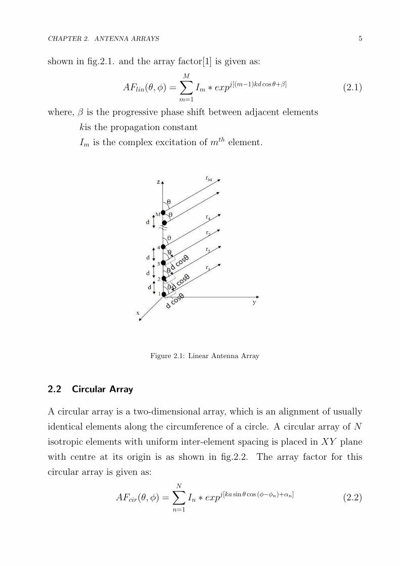
CHAPTER 2. ANTENNA ARRAYS 5
shown in fig.2.1. and the array factor[1] is given as:
AFlin(θ, φ) =
M∑
m=1
Im ∗ expj[(m−1)kd cos θ+β] (2.1)
where, β is the progressive phase shift between adjacent elements
kis the propagation constant
Im is the complex excitation of mth element.
Figure 2.1: Linear Antenna Array
2.2 Circular Array
A circular array is a two-dimensional array, which is an alignment of usually
identical elements along the circumference of a circle. A circular array of N
isotropic elements with uniform inter-element spacing is placed in XY plane
with centre at its origin is as shown in fig.2.2. The array factor for this
circular array is given as:
AFcir(θ, φ) =
N∑
n=1
In ∗ expj[ka sin θ cos (φ−φn)+αn] (2.2)

CHAPTER 2. ANTENNA ARRAYS 6
where, φn is the angular position of nth element on the circle
In is the excitation amplitude of nth element
αn is the excitation phase of nth element
a is the radius of the circle.
Figure 2.2: Circular Antenna Array
2.3 Conformal Arrays
The conformal arrays are three dimensional array that has radiating elements
following some prescribed shape. A conformal array is designed to integrate
on the curved surfaces for reduction of aerodynamic drag.
2.3.1 Spherical Array
The spherical antenna array is one of the conformal array of huge interest.
An adorable feature of the spherical antenna array is that, as its elements are
symmetrically aligned, the radiation pattern at any far field point over the
space will view the analogous environment. The spherical antenna array can

CHAPTER 2. ANTENNA ARRAYS 7
be operated to achieve multiple beam and shaped radiation patterns based
on signal processing and electronic beam steering capabilities.[3].
Figure 2.3: Spherical Antenna Array
Array Factor Formulation of Spherical Array
The spherical antenna array can be modelled as arrangement of circular ar-
rays one over the other. The radius of the circular arrays follows a definite
set of rules and decreases as we progress away from the centre of sphere.The
arrangement of spherical array is as shown in fig. 2.3.In this work a spherical
array is designed by alignment of 2M + 1 circular arrays of different radius
am and each circular array consists of Nm discrete and identical elements. As
the radius varies and to have the equal inter element spacing of the circular
array, the number of elements Nm varies for different circular array.The array
factor formth circular array of spherical array can be rewritten from equation
2.2 as:
AF (θ, φ) =
N∑
n=1
Inexp(jkam sin (θ) cos (φ−φn)+jψn) (2.3)
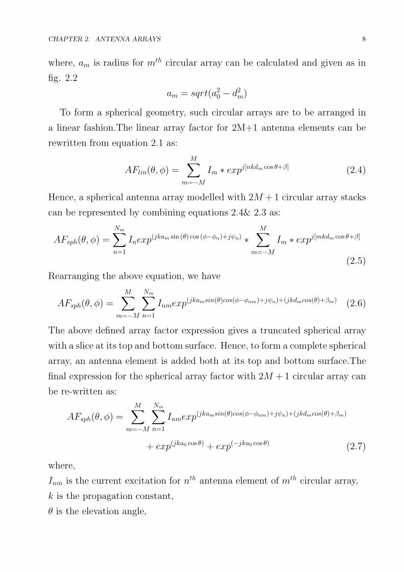
CHAPTER 2. ANTENNA ARRAYS 8
where, am is radius for mth circular array can be calculated and given as in
fig. 2.2
am = sqrt(a20 − d2m)
To form a spherical geometry, such circular arrays are to be arranged in
a linear fashion.The linear array factor for 2M+1 antenna elements can be
rewritten from equation 2.1 as:
AFlin(θ, φ) =M∑
m=−M
Im ∗ expj[nkdm cos θ+β] (2.4)
Hence, a spherical antenna array modelled with 2M +1 circular array stacks
can be represented by combining equations 2.4& 2.3 as:
AFsph(θ, φ) =
Nm∑
n=1
Inexp(jkam sin (θ) cos (φ−φn)+jψn) ∗
M∑
m=−M
Im ∗ expj[mkdm cos θ+β]
(2.5)
Rearranging the above equation, we have
AFsph(θ, φ) =M∑
m=−M
Nm∑
n=1
Inmexp(jkamsin(θ)cos(φ−φnm)+jψn)+(jkdmcos(θ)+βm) (2.6)
The above defined array factor expression gives a truncated spherical array
with a slice at its top and bottom surface. Hence, to form a complete spherical
array, an antenna element is added both at its top and bottom surface.The
final expression for the spherical array factor with 2M +1 circular array can
be re-written as:
AFsph(θ, φ) =M∑
m=−M
Nm∑
n=1
Inmexp(jkamsin(θ)cos(φ−φnm)+jψn)+(jkdmcos(θ)+βm)
+ exp(jka0 cos θ) + exp(−jka0 cos θ) (2.7)
where,
Inm is the current excitation for nth antenna element of mth circular array,
k is the propagation constant,
θ is the elevation angle,

CHAPTER 2. ANTENNA ARRAYS 9
φ is the azimuth angle,
φnm is the azimuth position of nth antenna element on mth circular array,
am is the radius for mth circle of spherical array and is given as in fig. ??:
am = sqrt(a20 − d2m)
a0 is the radius of spherical array,
ψn is the beam steering phase angle in azimuth direction,
dm is the distance of mth circular array from reference circular array at the
origin,
βm is the progressive phase shift between mth and reference circular array.
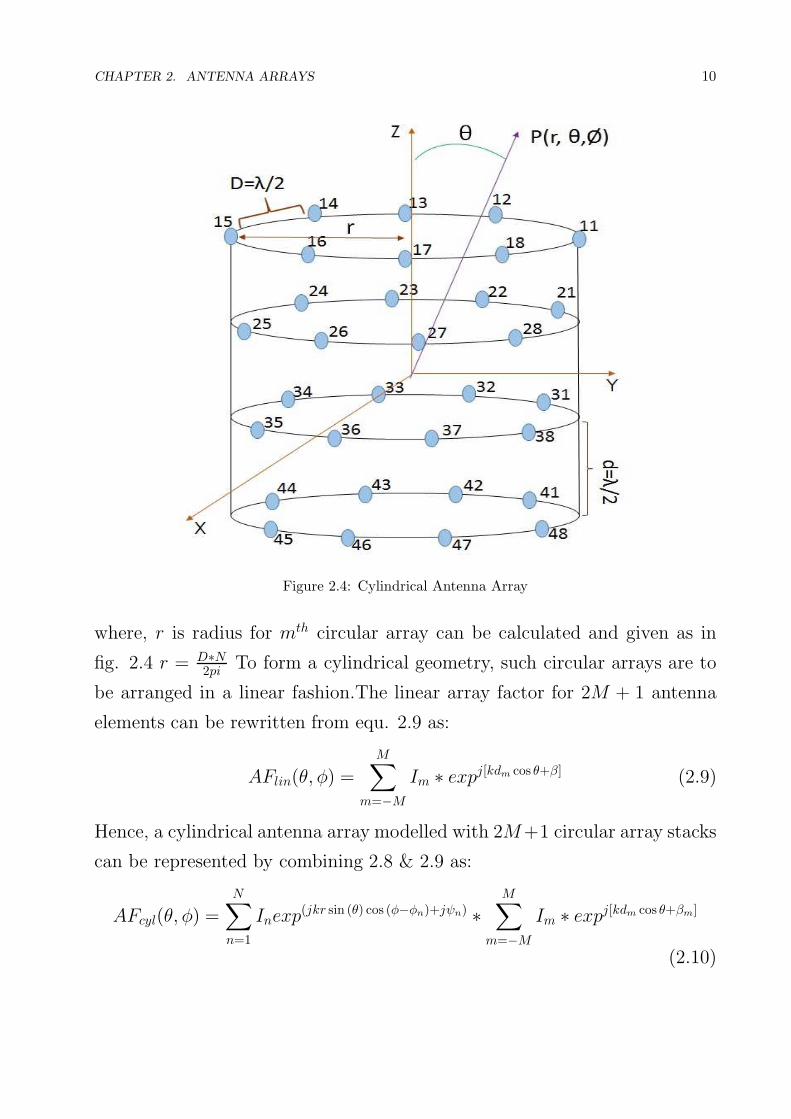
2.3.2 Cylindrical Array
An attractive feature of cylindrical array is that, any point in far-field the
beam is formed at the bisector of the cylindrical sector, and the cross-
polarizations caused by opposing elements in azimuth cancel each other. A
Cylindrical antenna array can be observed as a linear assembly of circular
array mounted one above the other such that the radius of all circular arrays
is constant as shown in Fig.2.4 . Hence, the basic foundation of cylindrical
array is taken from field equations of a circular array and linear array.
Array Factor Formulation of Cylindrical Array
For modelling cylindrical shaped array, the geometry can be viewed as it(cylindrical
array) is a linear stack arrangement of circular antenna array placed one
above the other such that the radius of all stacked circular arrays is constant
as given in fig. 2.4. Here, cylindrical array is modelled by taking 2M + 1
circular array of equal radius r in stack with each circular array consist of N
discrete and similar set of antenna elements. The array factor formth circular
array of cylindrical array can be rewritten from equ. 2.8 as:
AFcir(θ, φ) =
N∑
n=1
Inexp(jkr sin (θ) cos (φ−φn)+jψn) (2.8)
CHAPTER 2. ANTENNA ARRAYS 10
Figure 2.4: Cylindrical Antenna Array
where, r is radius for mth circular array can be calculated and given as in
fig. 2.4 r = D∗N2pi To form a cylindrical geometry, such circular arrays are to
be arranged in a linear fashion.The linear array factor for 2M + 1 antenna
elements can be rewritten from equ. 2.9 as:
AFlin(θ, φ) =
M∑
m=−M
Im ∗ expj[kdm cos θ+β] (2.9)
Hence, a cylindrical antenna array modelled with 2M+1 circular array stacks
can be represented by combining 2.8 & 2.9 as:
AFcyl(θ, φ) =N∑
n=1
Inexp(jkr sin (θ) cos (φ−φn)+jψn) ∗
M∑
m=−M
Im ∗ expj[kdm cos θ+βm]
(2.10)

CHAPTER 2. ANTENNA ARRAYS 11
Rearranging the above equation, we have
AFcyl(θ, φ) =M∑
m=−M
N∑
n=1
Inmexp(jkrsin(θ)cos(φ−φnm)+jψm)+(jkdmcos(θ)+βm) (2.11)
where,
Inm is the current excitation for nth antenna element of mth circular array,
k is the propagation constant,
θ is the elevation angle,
φ is the azimuth angle,
φnm is the azimuth position of nth antenna element on mth circular array,
r is the radius of circle of cylindrical array and is given as in fig. 2.4: r = D∗N2pi
ψm is the beam steering phase angle in azimuth direction,
dm is the distance of mth circular array from reference circular array at the
origin,
βm is the progressive phase shift between mth and reference circular array.
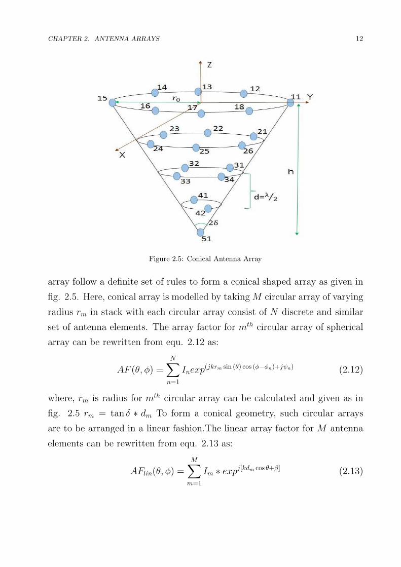
2.3.3 Conical Array
The cone array geometry, chosen for its similarity to an aircraft or missile nose
cone, is considered for several important performance parameters including
scan volume, side lobe control. A conical antenna array can be observed as a
linear assembly of circular array mounted one above the other such that the
radius of each circular array follow the property of cone as shown in Fig.2.5.
Hence, the Array factor formulation of conical array is derived from the array
factor of circular array and linear array.
Array Factor Formulation of Conical Array
For modelling conical shaped array, the geometry can be viewed as it(conical
array) is a linear stack arrangement of circular antenna array placed one
above the other such that, the radius of each progressive stacked circular
CHAPTER 2. ANTENNA ARRAYS 12
Figure 2.5: Conical Antenna Array
array follow a definite set of rules to form a conical shaped array as given in
fig. 2.5. Here, conical array is modelled by takingM circular array of varying
radius rm in stack with each circular array consist of N discrete and similar
set of antenna elements. The array factor for mth circular array of spherical
array can be rewritten from equ. 2.12 as:
AF (θ, φ) =N∑
n=1
Inexp(jkrm sin (θ) cos (φ−φn)+jψn) (2.12)
where, rm is radius for mth circular array can be calculated and given as in
fig. 2.5 rm = tan δ ∗ dm To form a conical geometry, such circular arrays
are to be arranged in a linear fashion.The linear array factor for M antenna
elements can be rewritten from equ. 2.13 as:
AFlin(θ, φ) =
M∑
m=1
Im ∗ expj[kdm cos θ+β] (2.13)

CHAPTER 2. ANTENNA ARRAYS 13
Hence, a spherical antenna array modelled with M circular array stacks can
be represented by combining 2.12 & 2.13 as:
AFcon(θ, φ) =
Nm∑
n=1
Inexp(jkrm sin (θ) cos (φ−φn)+jψn)∗
M∑
m=1
Im∗expj[kdm cos θ+β] (2.14)
Rearranging the above equation, we have
AFcon(θ, φ) =M∑
m=1
Nm∑
n=1
Inmexp(jkrmsin(θ)cos(φ−φnm)+jψn)+(jkdmcos(θ)+βm) (2.15)
The above defined array factor expression gives a truncated conical array
with a slice at its vertex. Hence, to form a complete conical array, an antenna
element is added vertex. The final expression for the conical array factor with
M circular array can be re-written as:
AFcon(θ, φ) =M∑
m=1
Nm∑
n=1
Inmexp(jkrmsin(θ)cos(φ−φnm)+jψn)+(jkdmcos(θ)+βm)+exp(−jkh cos θ)
(2.16)
where,
Inm is the current excitation for nth antenna element of mth circular array,
k is the propagation constant,
θ is the elevation angle,
φ is the azimuth angle,
φnm is the azimuth position of nth antenna element on mth circular array,
rm is the radius for mth circle of spherical array and is given as in fig. 2.5:
rm = tan δ ∗ dm
δ is the angle of conical array,
ψm is the beam steering phase angle in azimuth direction,
dm is the distance of mth circular array from origin,
βm is the progressive phase shift between mth and reference circular array.

Chapter 3
Cosecant Square Pattern
In modern technology, shaped-beams are widely used in satellite and radar
based applications. Cosecant-square pattern(CSP) is one such pattern which
is generally employed for long-range systems requiring higher gain near the
horizon with low gain at higher elevation angles. During detection of an air-
craft flying in space, it will be observed at a closer range at higher elevation
angles, so use of such pattern significantly limits the power available to air-
craft at higher elevation angles thereby providing a uniform signal strength
to the aircraft throughout its journey. Thus, the cosecant squared pattern
distribution [12] as shown in fig. 3.1 is a means of achieving a uniform signal
strength at the input of the receiver of target when it is moving at a constant
altitude.
3.1 Mathematical Justification of Cosecant-Squared Pattern
Consider an aircraft is flying at a constant height ’H’ in an Air Surveillance
radar System as shown in fig. ??. As it can be clearly observed that as the
aircraft is moving towards the radar system, its range ’R’ keeps on decreasing
with an increase in its elevation angle ’ε’. Thus, due to this continuous vari-
ation in the range of aircraft, the echo power received by radar receiver keeps
on changing. Thus, in order to receive uniform echo power by the receiver,
the radiation shape needs to be modified to Cosecant-square shape. It can
14

CHAPTER 3. COSECANT SQUARE PATTERN 15
(a) A Practical Cosecant-Squared pattern Refer-ence:radartutorial.eu
0 5 10 15 20 25 30 35−35
−30
−25
−20
−15
−10
−5
0
θ (degrees)
Des
ired(
in d
b)
(b) Simulated Cosecant-Squared pattern
Figure 3.1: Cosecant Square Radiation Pattern
be justified from the derivation as below:
The height H and the range R define the elevation angle ... By trigono-
metric relation, we have
R =H
sin(ε)⇒ R = Hcosec(ε) (3.1)
If the echo has a uniform signal strength at the input of the receiver than
Figure 3.2: Air surveillance Radar System

CHAPTER 3. COSECANT SQUARE PATTERN 16
the range is dependent on the square of the antenna gain in the fourth power
linearly.
Pr ∼G2
R4(3.2)
To receive uniform power by the aircraft Pr=constant Using above condition,
we have
G2 ∼ R4 (3.3)
which will be further reduced to,
G ∼ R2 (3.4)
Now using equation (3.1) in equ (3.4) we get,
G = (cosec(ε))2 (3.5)
3.2 Optimization Algorithms
The above discussed cosecant-squared pattern is one specific pattern and has
to be generated with various antenna arrays. To generate this pattern, we
requires some definite combination of radiation pattern controlling parame-
ters for array like excitation amplitude, phase, inter-element spacing etc so
that the newly generated radiation pattern tends to approximate the desired
radiation pattern. In present scenario, it is observed that many such prob-
lem statement requires efficient use of optimization algorithms [4] to reach
the desired solutions under various constraints. Nowadays, stochastic-based
optimization algorithms has become ineffective in several research areas. Due
to this, Evolutionary algorithms and Swarm-based optimization due to their
global behaviour and less number of controlling parameters are getting more
importance. Here, DE and SSO algorithms are discussed in details and are
applied to achieve the objective of this thesis.

CHAPTER 3. COSECANT SQUARE PATTERN 17
3.2.1 Differential Evolution Algorithm
Differential Evolution(DE) algorithm, proposed by Price and Storn in 1996, is
a stochastic population-based evolutionary algorithm [5] for optimizing multi-
dimensional space variables. In present scenario, there are so many problems
whose objective function are non-linear, noisy, flat and multi-dimensional
having more than one local minima and other constraints. Such problems are
difficult to solve analytically, hence DE based technique can be well utilized
to find an approximate result for such problems [10]. Moreover, compared to
other algorithms DE is more simpler and straightforward to implement with
very few control parameters (F, CR and N). It is extremely capable in pro-
viding multiple solutions in a single run with lower value of space complexity.
However, the convergence rate of DE algorithm is quite higher in comparison
to other class of algorithms [5]. This class of evolutionary algorithms follows
four basic steps [7, 6] as Initialization, Mutation, Recombination and Selec-
tion for its operation.
1. Initialization: To optimize a function with D real parameters, we
have to select a population of size N (at least of size 4)with the parameter
vector ’x’ given as:
xi, G = [x1,i,G, x2,i,G, ....... xD,i,G]
where, i = 1, 2, . . . , N
G is the generation number
The vector x is selected randomly from its bounded range [xLj , xUj ].
where, xLj is lower limit,
xUj is upper limit
After initialisation of every vector of the population, its corresponding fitness
value is computed and best of these is stored for future reference.
2. Mutation: Now for each given parameter xi,G, we will select three ran-
dom vectors xr1,G,xr2,G and xr3,G with distinct indices i, r1, r2 and r3. Apply

CHAPTER 3. COSECANT SQUARE PATTERN 18
mutation on it using equation as below:
vi,G+1 = xr1,G + F (xr2,G ∼ xr3,G)
where, F is the mutation factor, such that F∈[0,2]
vi,G+1 is called as donar vector
3. Recombination: Now recombination uses successful solutions obtained
from the previous generation and generates a new trial vector from the ele-
ments of the previous target vector xi,G and the elements of the newly created
donar vector vi,G+1 based on the following relation:
uj,i,G+1 =
vj,i,G+1, if randj,i ≤ CR or j = Irand
xj,i,G, if randj,i > CR and j 6= Irand
where,i = 1, 2, . . . , N ;
j = 1, 2, . . . , D
Irand is a random integer[1,2,......D] such that, vi,G+1 6= xj,i,G
4. Selection: Finally, selection for next generation vector is done by com-
paring fitness value due to trial vector vi,G+1 and target vector xi,G using
criteria
xi,G+1 =
xi,G+1, if f(u1,G+1) ≤ f(x1,G)
xi,G, otherwise
Now, the process of Mutation, Recombination and Selection is repeated till
some stopping criterion as defined in the algorithm is reached.
The concept of DE algorithm process is presented with the flowchart [11]
shown by fig. 3.3 as:

CHAPTER 3. COSECANT SQUARE PATTERN 19
Start Differential Evolution
Generation g=1
initialize NPxD populationThe excitation parameter is considered as population αg,i =[
αg,i1
, αg,i2
, . . . , αg,i
D
]T, i = 1, 2, . . . , NP, g = 1, 2, . . . , Gd
Is TerminationCriterian Met Finish DE
Take best individual as solution
αbest = argminn
(
fGd,n
fitness
(
αGd,n))
Mutation
Crossover
Evolution: E1 = fg,n
fitness(ug,n)
Evolution: E2 = fg,n
fitness(αg,n)
IsE1 ≤ E2
αg,n = αg,n
αg,n = ug,n
g = g + 1
Yes
No
Yes
No
Figure 3.3: Flowchart of Differential Evolution Algorithm

CHAPTER 3. COSECANT SQUARE PATTERN 20
Validation of DE with the Published Work
Referred to [23] of Symmetric Linear array with 24 elements with uniform
spacing of 0.5λ to minimise the SLL value. It is observed from the paper that
GA optimization algorithm gives a SLL of -34.5dB with excitation amplitude
optimization. Applying same constraints as mentioned in [23] with DE algo-
rithm having parameters as mentioned in Table3.1, it is observed from fig.
3.4 that SLL reaches a value of -38.42dB for amplitude variation as indicated
in Table 3.2.
Table 3.1: Parameters Used for DE Validation
S No. Parameters Value
1 Number of Elements 24
2 Inter-element Spacing 0.5λ
3 Population Size 50
4 Iterations 1000
5 θMLL (76,104)
6 θSLL [0,76]&[104,180]
7 F 0.8CR 0.3VTR 0
0 20 40 60 80 100 120 140 160 180−50
−45
−40
−35
−30
−25
−20
−15
−10
−5
0
θ (degrees)
Ga
in(d
B)
Radiation Pattern
DEKhodier
(a) Radiation Pattern Comparision
−12−11−10−9 −8 −7 −6 −5 −4 −3 −2 −1 0 1 2 3 4 5 6 7 8 9 10 11 120
0.1
0.2
0.3
0.4
0.5
0.6
0.7
0.8
0.9
1
Element #
No
rma
lise
d A
mp
litu
de
DEKhodier
(b) Normalized amplitude distribution |In| of array ele-ments
Figure 3.4: DE and PSO(Khodier) for N=24 Symmetric Linear Array

CHAPTER 3. COSECANT SQUARE PATTERN 21
Table 3.2: Performance Comparison between DE and PSO (Khodier)
Algorithms Normalised Amplitude(In) SLL(in dB)
PSO(Khodier) 1.0000,0.9712,0.9226,0.8591,0.7812,0.6807 -34.50.5751,0.4768,0.3793,0.2878,0.2020,2167
DE 1.0000,0.9454,0.8709,0.8288,0.6783,0.5676 -38.420.4699,0.3457,0.2525,0.1695,0.0852,0.0355
3.2.2 Simplified Swarm Optimization Algorithm
Simplified Swarm optimization(SSO) is an emerging met-heuristic algorithm
which searches for best values with the help of population (swarm) of individ-
uals (particles) which gets updated to better values with each iterations. It
is derived from Particle Swarm optimization(PSO), as a simplified version of
PSO technique It is designed to remove the premature convergence of PSO in
high-dimensional multi-modal problems [8, 9]. Thus, SSO is able to improve
the convergence speed with increase in number of iterations. SSO starts with
some size of swarm population having random position of particles, maxi-
mum number of generations and three controlling parameters Cw, Cp & Cg
depending on the application. In every generation, the particle’s position
value in each dimension keeps on updating to some new pbest value or gbest
value or some random value according to following criteria as under [8]:
xtid =
xt−1i , if rand() ∈ [0, Cw)
pt−1i , if rand() ∈ [Cw, Cp)
gt−1i , if rand() ∈ [Cp, Cg)
x, if rand() ∈ [Cg, 1)
here, i=1,2,......m; where m is size of swarm
Xi = (xi1, xi1, ...... xiD)
where, xiD is the position value of the ith particle for Dth space dimension.
Cw, Cp & Cg are three constant positive parameters such that
Cw < Cp < Cg

CHAPTER 3. COSECANT SQUARE PATTERN 22
Pi = (pi1, pi1, ...... piD) denotes the best solution achieved by each individuals
(pbest),
Gi = (gi1, gi1, ...... giD) denotes the best solution achieved so far by the whole
swarms (gbest),
x represents the new value for the particle in every dimension which are ran-
domly generated from random function ’rand()’; where, the random number
can be taken between 0 and 1.
The SSO algorithm is explained in detail by the flowchart fig. 3.5 shown
below:
Validation of SSO
Referred to AF of circular array [14] of 30 isotropic elements with inter-
element spacing of 0.5λ, optimization based on SSO algorithm has been ap-
plied under mentioned constraints and compared with GA results to show
the superiority of SSO over GA. The various parameters considered for this
comparison [14] are shown in Table 3.3. It is observed from the simulated
result fig. 3.6 & Table 3.4 that there is a drastic reduction in side lobe
level which reduces from -10.88dB with Genetic algorithm used in [14] to a
value of -13.11dB with the proposed SSO algorithm. Moreover, no ripples
are observed with proposed scheme showing an upper hand of the proposed
scheme.
Table 3.3: Parameters Used for SSO Validation
S No. Parameters Value
1 Number of Elements 30
2 Inter-element Spacing 0.5λ
3 Population Size 50
4 Iterations 500
5 θCSC (0,30)
6 θSLL (-90,0)&(30,90)
7 Cg [0.45,0.65]Cp (0.65,0.85]Cw (0.85,0.95]

CHAPTER 3. COSECANT SQUARE PATTERN 23
Start
initialization: m = swarm sizeCw, Cp, Cg = constant parametersmaxGen = maximum generationmaxFit = maximum fitness value
generate and initialize pbest andgbest with random position x
Evaluate fitness-value for each particle
Update pbest and gbest
generate random number
0≤R< Cw keep the original value
Cw ≤R<
Cpreplace value by pbest
Cp ≤R< Cg replace value by gbest
randomly generate new valueto replace the original value
meetterminationcriteria?
Stop
Yes
Yes
Yes
Yes
no
Figure 3.5: Flowchart of SSO Algorithm

CHAPTER 3. COSECANT SQUARE PATTERN 24
Table 3.4: Desired & Obtained Results
Parameter Desired GA SSO
SLL(in dB) -15 -10.88 -13.11
−80 −60 −40 −20 0 20 40 60 80−20
−18
−16
−14
−12
−10
−8
−6
−4
−2
0
θ(in degree)
AF
Gai
n(in
db)
Radiation Pattern
DesiredDEGA
(a) Radiation Pattern
0 100 200 300 400 5001.5
2
2.5
3
3.5
4
4.5
5
5.5
Iterations
Cos
t Fun
ctio
n
SSO
(b) SSO Cost Function
Figure 3.6: Comparison Result between SSO & GA for N=30 Circular Array
3.3 Simulation Results for Cosecant Square Pattern
Applying basic Differential evolution(DE) and Simple Swarm optimization(SSO)
algorithms on linear, circular and spherical array, cosecant-squared pattern
is generated. The desired pattern used for all three conformal arrays is as
shown in fig.3.7 is plotted against azimuthal angle φ with a cosecant-squared
curve of 45◦.
The calculation of ripple component in the obtained cosec2 pattern is given
by cumulative summation of the deviation ∆ripple in cosecant curve from de-
sired curve as :
∆ripple = ∆CSC =∑
θ∈[cscrange]
|AF (θ, 90)−Desired(θ, 90)| (3.6)

CHAPTER 3. COSECANT SQUARE PATTERN 25
0 50 100 150 200 250 300 350−25
−20
−15
−10
−5
0
φ (degrees)
Ga
in(d
B)
Radiation pattern
Desired
Figure 3.7: Desired CSP for all three Conformal Antenna Array
3.3.1 Case Study 1: Spherical Array
An array factor of spherical array with 184,260 & 376 isotropic elements
placed such that 26,34 & 50 elements are in main circular array, 156, 224
&324 elements are arranged in twelve sub-circular arrays and single element
is at the top and the bottom as in equation (4.1) with Inm optimization is
considered:
AFsph(θ, φ) =
M∑
m=−M
Nm∑
n=1
Inmexp(jkamsin(θ)cos(φ−φnm)+jψn)+(jkdmcos(θ)+βm)
+ exp(jka0 cos θ) + exp(−jka0 cos θ) (3.7)
where,
Inm = |Inm|ejψn is the current excitation for nth antenna element of mth
circular array,
|Inm| is the normalised amplitude and ψn is the phase of excitation,
φnm is the azimuth position of nth antenna element on mth circular array,
am is the radius for mth circle of spherical array,
a0 is the radius of spherical array,
dm is the distance of mth circular array from reference circular array at the
origin,

CHAPTER 3. COSECANT SQUARE PATTERN 26
The fitness function used for spherical array is given by equation as:
fcost = α ∗∆CSC + β ∗∆SLL + γ ∗∆ (3.8)
where, ∆ =∑
φ∈[0,360] |AF (90, φ)−Desired(90, φ)|
∆CSC =∑
φ∈[181,225] |AF (90, φ)−Desired(90, φ)|
∆SLL =∑
φ∈[0,180]&[226,360] |AF (90, φ)−Desired(90, φ)|
To reduce the ripple in main lobe level the values of α, βandγ values are taken
as 0.875,0.125 and 0.00 respectively.
0 50 100 150 200 250 300 350
−25
−20
−15
−10
−5
0
φ (degrees)
Ga
in(d
B)
Radiation pattern
IDEALDESSO
(a) Radiation Pattern for N=376 Elements
0 100 200 300 400 500 600 700 800 900 10001.5
2
2.5
3
3.5
4
4.5
5
5.5
Iterations
Fitn
ess(
dB)
Cost Function
DESSO
(b) Cost Function for N=376 Elements
Figure 3.8: Results of Spherical Array with 376 elements
From the simulation results fig 3.8, fig.3.9 & fig.3.10 it can be understand
that cosecant squared pattern is synthesised well in main lobe by using spher-
ical antenna array with different number of elements.
From the cost function figures shows that the amount of convergence is not
following particular relation with the number of elements. From all the three
figures it is clear that the rate of convergence for sso algorithm is better than
the de algorithm.
The amount of convergence between DE and SSO is incomparable as it is
different for different set of elements.

CHAPTER 3. COSECANT SQUARE PATTERN 27
0 50 100 150 200 250 300 350−25
−20
−15
−10
−5
0
φ (degrees)
Gain(dB
)
Radiation pattern
IDEALDESSO
(a) Radiation Pattern for N=260 Elements
0 100 200 300 400 500 600 700 800 900 10001.4
1.6
1.8
2
2.2
2.4
2.6
2.8
3
3.2
Iterations
Fitn
ess(d
B)
Cost Function
DESSO
(b) Cost Function for N=260 Elements
Figure 3.9: Results of Spherical Array with 260 elements
0 50 100 150 200 250 300 350−25
−20
−15
−10
−5
0
φ (degrees)
Ga
in(d
B)
Radiation pattern
IDEALDESSO
(a) Radiation Pattern for N=184 Elements
0 100 200 300 400 500 600 700 800 900 10001.5
2
2.5
3
3.5
4
Iterations
Finess(dB
)
Cost Function
DESSO
(b) Cost Function for N=184 Elements
Figure 3.10: Results of Spherical Array with 184 elements
3.3.2 Case Study 2: Cylindrical Array
An array factor of cylindrical array with 182,286 & 390 isotropic elements
placed such that 14,22 & 30 elements are in each circular array. A linear
arrangement of 13 such circular arrays is as in equation (3.9) with Inm opti-

CHAPTER 3. COSECANT SQUARE PATTERN 28
mization is considered:
AFcyl(θ, φ) =
M∑
m=−M
N∑
n=1
Inmexp(jkrsin(θ)cos(φ−φnm)+jψm)+(jkdmcos(θ)+βm) (3.9)
where,
Inm = |Inm|ejψn is the current excitation for nth antenna element of mth
circular array,
|Inm| is the normalised amplitude and ψn is the phase of excitation,
φnm is the azimuth position of nth antenna element on mth circular array,
r is the radius of cylindrical array,
dm is the distance of mth circular array from reference circular array at the
origin,
The fitness function used for spherical array is given by equation as:
fcost = α ∗∆CSC + β ∗∆SLL + γ ∗∆ (3.10)
where, ∆ =∑
φ∈[0,360] |AF (90, φ)−Desired(90, φ)|
∆CSC =∑
φ∈[181,225] |AF (90, φ)−Desired(90, φ)|
∆SLL =∑
φ∈[0,180]&[226,360] |AF (90, φ)−Desired(90, φ)|
To reduce the ripple in main lobe level the values of α, βandγ values are taken
as 0.875,0.125 and 0.00 respectively.
It is observed from the simulation results fig 3.11, fig3.12 & fig 3.13 that it
can be understand that cosecant squared pattern is synthesised well in main
lobe by using cylindrical antenna array with different number of elements.
From the cost function figures it is clear that as the number of elements
decreases, the better cosecant square radiation pattern is achieved.
From all the three figures it is clear that the rate of convergence is better for
sso algorithm and amount of convergence is better for DE.
3.3.3 Case Study 3: Conical Array
An array factor of conical array with 195,291 & 381 isotropic elements placed
such that 32,44 & 56 elements are in main circular array and 162, 246 & 324

CHAPTER 3. COSECANT SQUARE PATTERN 29
0 50 100 150 200 250 300 350−25
−20
−15
−10
−5
0
φ (degrees)
Ga
in
(d
B)
Radiation pattern
IDEALDESSO
(a) Radiation Pattern for N=390 Elements
0 100 200 300 400 500 600 700 800 900 10001
1.5
2
2.5
3
3.5
4
4.5
Iterations
Fitn
ess(d
B)
Cost Function
DESSO
(b) Cost Function for N=390 Elements
Figure 3.11: Results of Cylindrical Array with 390 elements
0 50 100 150 200 250 300 350−25
−20
−15
−10
−5
0
5
10
φ (degrees)
Ga
in(d
B)
Radiation pattern
IDEALDESSO
(a) Radiation Pattern for N=286 Elements
0 100 200 300 400 500 600 700 800 900 10001
1.5
2
2.5
3
3.5
4
Iterations
Fitness (dB
)
Cost Function
DESSO
(b) Cost Function for N=286 Elements
Figure 3.12: Results of Cylindrical Array with 286 elements
elements are arranged in twelve sub-circular arrays and single element is at
the vertex as in equation (4.3) with Inm optimization is considered:
AFcon(θ, φ) =M∑
m=1
Nm∑
n=1
Inmexp(jkrmsin(θ)cos(φ−φnm)+jψn)+(jkdmcos(θ)+βm)+exp(−jkh cos θ)
(3.11)

CHAPTER 3. COSECANT SQUARE PATTERN 30
0 50 100 150 200 250 300 350−25
−20
−15
−10
−5
0
φ (degrees)
Ga
in (d
B)
Radiation pattern
IDEALDESSO
(a) Radiation Pattern for N=182 Elements
0 100 200 300 400 500 600 700 800 900 10001
1.5
2
2.5
3
3.5
4
4.5
5
Iterations
Fitness (dB
)
Cost Function
DESSO
(b) Cost Function for N=182 Elements
Figure 3.13: Results of Cylindrical Array with 182 elements
where,
Inm = |Inm|ejψn is the current excitation for nth antenna element of mth
circular array,
|Inm| is the normalised amplitude and ψn is the phase of excitation,
φnm is the azimuth position of nth antenna element on mth circular array,
rm is the radius for mth circle of conical array,
h is the height of conical array,
dm is the distance of mth circular array from reference circular array at the
origin,
The fitness function used for conical array is given by equation as:
fcost = α ∗∆CSC + β ∗∆SLL + γ ∗∆ (3.12)
where, ∆ =∑
φ∈[0,360] |AF (90, φ)−Desired(90, φ)|
∆CSC =∑
φ∈[181,225] |AF (90, φ)−Desired(90, φ)|
∆SLL =∑
φ∈[0,180]&[226,360] |AF (90, φ)−Desired(90, φ)|
To reduce the ripple in main lobe level the values of α, βandγ values are taken
as 0.875,0.125 and 0.00 respectively.
The simulation results in fig 3.14, fig3.15 & fig3.16 shows that the squared

CHAPTER 3. COSECANT SQUARE PATTERN 31
0 50 100 150 200 250 300 350−25
−20
−15
−10
−5
0
φ (degrees)
Ga
in(d
B)
Radiation pattern
IDEALDESSO
(a) Radiation Pattern for N=381 Elements
0 100 200 300 400 500 600 700 800 900 10001.4
1.6
1.8
2
2.2
2.4
2.6
2.8
3
3.2
Iterations
Fitn
ess(d
B)
Cost Function
DESSO
(b) Cost Function for N=381 Elements
Figure 3.14: Results of Conical Array with 381 elements
0 50 100 150 200 250 300 350−25
−20
−15
−10
−5
0
5
10
φ (degrees)
Ga
in(d
B)
Radiation pattern
IDEALDESSO
(a) Radiation Pattern for N=291 Elements
0 100 200 300 400 500 600 700 800 900 10001.5
2
2.5
3
3.5
4
4.5
5
5.5
Iterations
Fitn
ess(d
B)
Cost Function
DESSO
(b) Cost Function for N=291 Elements
Figure 3.15: Results of Conical Array with 291 elements
pattern is synthesised better in main lobe by using conical antenna array
with different number of elements.
From the cost function figures it is clear that as the number of elements in-
creases the better cosecant square radiation pattern is achieved.
But the amount of convergence and rate of convergence doesnt follow any
relation between DE and SSO.

CHAPTER 3. COSECANT SQUARE PATTERN 32
0 50 100 150 200 250 300 350−30
−25
−20
−15
−10
−5
0
φ (degrees)
Ga
in(d
B)
Radiation pattern
IDEALDESSO
(a) Radiation Pattern for N=195 Elements
0 100 200 300 400 500 600 700 800 900 10001.5
2
2.5
3
3.5
4
4.5
5
5.5
6
Iterations
Fitn
ess (d
B)
Cost Function
DESSO
(b) Cost Function for N=195 Elements
Figure 3.16: Results of Conical Array with 195 elements
Table 3.5: Performance Comparison of Conformal arrays
comparison Spherical Array as Cylindrical Array as Conoical Array asParameter No. of Elements No. of Elements No. of Elements
increases increases increases
Rate of convergenceSSO > DE SSO > DE −−−
w.r.t No. of elements
Amount of convergence−−− Decreases Increases
w.r.t No. of elements
Amount of convergence−−− DE > SSO −−−
w.r.t algorithms
where −−− indicates there is no particular trend.

Chapter 4
Impact of Azimuthal Plane Elements
4.1 Problem Formulation
The cosecant squared pattern is synthesized by linear antenna array [13] and
also by conformal antenna arrays.There is a significant difference in num-
ber of elements in linear and conformal array for the generation of cosecant
squared radiation pattern. To bridge this gap, only elements in an azimuthal
plane of conformal antenna array are excited based on the mask generated for
that azimuthal plane constraint, and the cosecant squared radiation pattern
is synthesized. The excitation parameters of the conformal array elements
are optimized using DE & SSO optimization techniques.
4.2 Selection of Azimuthal Plane
For selecting the elements in azimuthal plane,the position coordinates of the
existing elements are used to generate the mask and masking is done for the
elements. The procedure for selecting the azimuthal plane for best radiation
pattern is as shown in flowchart.
33

CHAPTER 4. IMPACT OF AZIMUTHAL PLANE ELEMENTS 34
Start
Initialization: Azimuthal plane φ = 0
Generate the mask for the azimuthal plane based on mask
Switching the elements based on mask
Optimize the excitation of elements with DE and SSO algorithms
Obtain Cost Function(CF) value and Radiation Pattern(RP)
Select the other azimuthal plane by φ = φ + 5
CFn+1 <
CFn
Update the best azimuthal plane
φ ≤ 360
Fetch the best azimuthal plane
Stop
Yes
no
no
yes
Figure 4.1: Procedure for Selection of Best Azimuthal Plane

CHAPTER 4. IMPACT OF AZIMUTHAL PLANE ELEMENTS 35
4.3 Pattern Synthesis with Different Azimuthal Plane Elements
4.3.1 Case1: Spherical Array
For selecting the elements in azimuthal plane,the position coordinates of the
existing elements are used to generate the mask and masking is done for the
elements. The procedure for selecting the azimuthal plane for best radiation
pattern is as shown in fig.4.1.E is the mask generated for the φ plane which
generates the radiation pattern closer to the desired pattern.The array factor
of the spherical array with the selected elements is the product of masking
coefficient and the spherical array factor as in equation 4.1 and final equation
is given as
AFsph(θ, φ) =
M∑
m=−M
Nm∑
n=1
Enm ∗ Inmexp(jkamsin(θ)cos(φ−φnm)+jψn)+(jkdmcos(θ)+βm)
+ exp(jka0 cos θ) + exp(−jka0 cos θ) (4.1)
where Enm is the masking coefficient for nth antenna element of mth circular
array,
After masking, the selected elements of a particular azimuthal plane of the
Figure 4.2: Spherical Antenna Array with Selection
spherical array can be viewed as shown in fig.4.2. The excitation parame-

CHAPTER 4. IMPACT OF AZIMUTHAL PLANE ELEMENTS 36
ters of the selected elements are optimised using the DE and SSO algorithms.
Fig.4.3 and fig.4.4 are the simulation results when φ = 180◦ plane elements,
φ = 355◦ plane elements got selected over the spherical array respectively.
From the Fig.4.3 & FIg,4.4 it can easily noted that every φ plane selection
will not be able to radiate the cosecant square pattern.
0 50 100 150 200 250 300 350−25
−20
−15
−10
−5
0
φ (degrees)
Ga
in(d
B)
Radiation pattern
IDEALDESSO
(a) Radiation Pattern for best ( phi = 180◦) Plane Elements
0 100 200 300 400 500 600 700 800 900 10001
1.2
1.4
1.6
1.8
2
2.2
2.4
2.6
2.8
Iterations
Fitn
ess(d
B)
Cost Function
DESSO
(b) Cost Function for best ( phi = 180◦) Plane Elements
Figure 4.3: Results of Spherical Array for Best ( phi = 180◦) Plane Elements
From the Fig.4.3, clearly shows that the cosecant square pattern synthe-
sis is done with the elments got selected over the phi = 180◦ plane of the
spherical array.
From the Fig.4.4,shows that the radiation pattern of the elments got se-
lected over the phi = 355◦ plane of the spherical array have more sidelobe
levels and the main beam of CSP is also not synthesised.
4.3.2 Case2: Cylindrical Array
A mask is generated for the selection of elements of the cylindrical array in a
particular φ plane with the procedure shown in flow chart4.1.E is the mask

CHAPTER 4. IMPACT OF AZIMUTHAL PLANE ELEMENTS 37
0 50 100 150 200 250 300 350−25
−20
−15
−10
−5
0
φ (degrees)
Ga
in(d
B)
Radiation pattern
IDEALDESSO
(a) Radiation Pattern for worst ( phi = 355◦) Plane Elements
0 100 200 300 400 500 600 700 800 900 10004.7
4.8
4.9
5
5.1
5.2
5.3
5.4
5.5
5.6
5.7
Iterations
Fitn
ess (d
B)
Cost Function
DESSO
(b) Cost Function for worst ( phi = 355◦) Plane Elements
Figure 4.4: Results of Spherical Array for Worst ( phi = 355◦) Plane Elements
generated for the φ plane which generates the radiation pattern closer to
the desired pattern.The array factor of the cylindrical array with the selected
elements, is the product of masking coefficient and the cylindrical array factor
as in equation 3.9 and final equation is given as
AFcyl(θ, φ) =M∑
m=−M
N∑
n=1
Enm ∗ Inmexp(jkrsin(θ)cos(φ−φnm)+jψm)+(jkdmcos(θ)+βm)
(4.2)
where Enm is the masking coefficient for nth antenna element of mth circular
array,
The finally selected elements are of desired azimuthal plane as shown in Fig.
4.5 for cylindrical array.The excitation parameters of the selected elements
are optimised using the DE and SSO algorithms.
Fig.4.6 and fig.4.7 are the simulation results when φ = 255◦ plane elements,
φ = 0◦ plane elements got selected over the spherical array respectively. From
the Fig.4.6 & FIg,4.7 it can easily noted that every φ plane selection will not
be able to radiate the cosecant square pattern.
From the Fig.4.6, clearly shows that the cosecant square pattern synthesis

CHAPTER 4. IMPACT OF AZIMUTHAL PLANE ELEMENTS 38
Figure 4.5: Cylindrical Antenna Array with Selection
0 50 100 150 200 250 300 350−25
−20
−15
−10
−5
0
φ (degrees)
Ga
in(d
B)
Radiation pattern
IDEALDESSO
(a) Radiation Pattern for best ( phi = 255◦) Plane Elements
0 100 200 300 400 500 600 700 800 900 10001
1.5
2
2.5
3
3.5
4
4.5
Iterations
Fitness(dB
)
Cost Function
DESSO
(b) Cost Function for best ( phi = 255◦) Plane Elements
Figure 4.6: Results of Cylindrical Array for Best ( phi = 255◦) Plane Elements
is done with the elements got selected over the phi = 255◦ plane of the
cylindrical array.
From the Fig.4.7,shows that the radiation pattern of the elements got

CHAPTER 4. IMPACT OF AZIMUTHAL PLANE ELEMENTS 39
0 50 100 150 200 250 300 350−25
−20
−15
−10
−5
0
φ (degrees)
Ga
in(d
B)
Radiation pattern
IDEALDESSO
(a) Radiation Pattern for worst ( phi = 0◦) Plane Elements
0 100 200 300 400 500 600 700 800 900 10004.5
5
5.5
6
6.5
Iterations
Fitness(dB
)
Cost Function
DESSO
(b) Cost Function for worst ( phi = 0◦) Plane Elements
Figure 4.7: Results of Cylindrical Array for Worst ( phi = 0◦) Plane Elements
selected over the phi = 0◦ plane of the cylindrical array have more side lobe
levels and the main beam of CSP is also not synthesised.
4.3.3 Case3: Conical Array
For selecting the elements in azimuthal plane,the position coordinates of the
existing elements are used to generate the mask and masking is done for the
elements. The procedure for selecting the azimuthal plane for best radiation
pattern is as shown in fig.4.1.E is the mask generated for the φ plane which
generates the radiation pattern closer to the desired pattern.The array factor
of the conical array with the selected elements is the product of masking
coefficient and the conical array factor as in equation 4.3 and final equation
is given as
AFcon(θ, φ) =
M∑
m=1
Nm∑
n=1
EnmInmexp(jkrmsin(θ)cos(φ−φnm)+jψn)+(jkdmcos(θ)+βm)+exp(−jkh cos θ)
(4.3)
where Enm is the masking coefficient for nth antenna element of mth circular
array,
The finally selected elements are of desired azimuthal plane as shown in Fig.
4.8 for conical array.The excitation parameters of the selected elements are

CHAPTER 4. IMPACT OF AZIMUTHAL PLANE ELEMENTS 40
Figure 4.8: Conical Antenna Array with Selection
optimised using the DE and SSO algorithms.
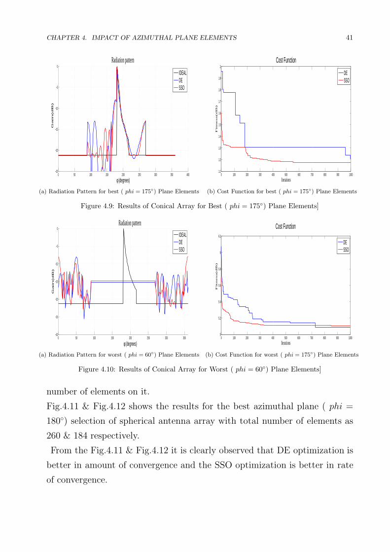
Fig.4.9 and fig.4.10 are the simulation results when φ = 175◦ plane elements,
φ = 60◦ plane elements got selected over the spherical array respectively.
From the Fig.4.9 & Fig,4.10 it can easily noted that every azimuthal plane
selection will not be able to radiate the cosecant square pattern.
From the Fig.4.9, clearly shows that the cosecant square pattern synthesis
is done with the elements got selected over the phi = 175◦ plane of the
cylindrical array.
From the Fig.4.10,shows that the radiation pattern of the elements got
selected over the phi = 60◦ plane of the cylindrical array have more side
lobe levels and the main beam of CSP is also not synthesised.
4.4 Pattern Synthesis with Best Azimuthal Plane Elements
4.4.1 Case4: Spherical Array with different set of elements
The procedure for selecting the azimuthal plane for best radiation pattern is
as shown in fig.4.1, is done for the spherical antenna array with 260 and 184
CHAPTER 4. IMPACT OF AZIMUTHAL PLANE ELEMENTS 41
0 50 100 150 200 250 300 350 400−25
−20
−15
−10
−5
0
φ (degrees)
Ga
in(d
B)
Radiation pattern
IDEALDESSO
(a) Radiation Pattern for best ( phi = 175◦) Plane Elements
0 100 200 300 400 500 600 700 800 900 10001.1
1.2
1.3
1.4
1.5
1.6
1.7
1.8
1.9
2
Iterations
Fitn
ess(d
B)
Cost Function
DESSO
(b) Cost Function for best ( phi = 175◦) Plane Elements
Figure 4.9: Results of Conical Array for Best ( phi = 175◦) Plane Elements]
0 50 100 150 200 250 300 350−30
−25
−20
−15
−10
−5
0
φ (degrees)
Ga
in(d
B)
Radiation pattern
IDEALDESSO
(a) Radiation Pattern for worst ( phi = 60◦) Plane Elements
0 100 200 300 400 500 600 700 800 900 10005
5.2
5.4
5.6
5.8
6
6.2
Iterations
Fitn
ess(d
B)
Cost Function
DESSO
(b) Cost Function for worst ( phi = 175◦) Plane Elements
Figure 4.10: Results of Conical Array for Worst ( phi = 60◦) Plane Elements]
number of elements on it.
Fig.4.11 & Fig.4.12 shows the results for the best azimuthal plane ( phi =
180◦) selection of spherical antenna array with total number of elements as
260 & 184 respectively.
From the Fig.4.11 & Fig.4.12 it is clearly observed that DE optimization is
better in amount of convergence and the SSO optimization is better in rate
of convergence.

CHAPTER 4. IMPACT OF AZIMUTHAL PLANE ELEMENTS 42
0 50 100 150 200 250 300 350−25
−20
−15
−10
−5
0
φ (degrees)
Ga
in(d
B)
Radiation pattern
IDEALDESSO
(a) Radiation Pattern for best ( phi = 180◦) Plane Elements
0 100 200 300 400 500 600 700 800 900 10001
1.5
2
2.5
3
3.5
Iterations
Fitness(dB
)
Cost Function
DESSO
(b) Cost Function for best ( phi = 180◦) Plane Elements
Figure 4.11: Results of Spherical Array for Best ( phi = 180◦) Plane Elements
0 50 100 150 200 250 300 350−25
−20
−15
−10
−5
0
φ (degrees)
Ga
in(d
B)
Radiation pattern
IDEALDESSO
(a) Radiation Pattern for best ( phi = 180◦) Plane Elements
0 100 200 300 400 500 600 700 800 900 10001
1.5
2
2.5
3
3.5
Iterations
Fitness(dB
)
Cost Function
DESSO
(b) Cost Function for best ( phi = 180◦) Plane Elements
Figure 4.12: Results of Spherical Array for Best ( phi = 180◦) Plane Elements
4.4.2 Case5: Cylindrical Array with different set of elements
The procedure for selecting the azimuthal plane for best radiation pattern is
as shown in fig.4.1, is done for the cylindrical antenna array with 286 and
182 number of elements on it.
Fig.4.13 & Fig.4.14 shows the results for the best azimuthal plane ( phi =
255◦) selection of cylindrical antenna array with total number of elements as
286 & 182 respectively.

CHAPTER 4. IMPACT OF AZIMUTHAL PLANE ELEMENTS 43
Table 4.1: Performance Comparison for Spherical Array
all elements seletion phi = 180◦ selected
No. of ele.DE SSO
No. of ele.DE SSO
ripple(dB) ripple(dB) ripple(dB) ripple(dB)
376 0.6411 0.9733 13 0.2387 0.7215
260 0.7524 0.9639 12 0.286 0.8218
184 0.9 1.02 12 0.2468 0.789
Fig.4.13 clearly shows that the amount of convergence for both DE and SSO
0 50 100 150 200 250 300 350 400−25
−20
−15
−10
−5
0
φ (degrees)
Ga
in(d
B)
Radiation pattern
IDEALDESSO
(a) Radiation Pattern for best ( phi = 255◦) Plane Elements
0 100 200 300 400 500 600 700 800 900 10001
1.2
1.4
1.6
1.8
2
2.2
2.4
2.6
2.8
Iterations
Fitness (
dB
)
Cost Function
DESSO
(b) Cost Function for best ( phi = 255◦) Plane Elements
Figure 4.13: Results of Cylindrical Array for Best ( phi = 255◦) Plane Elements
optimizations is approximately same for phi = 255◦ Plane on cylindrical ar-
ray with 286 elements.
Fig.4.14 clearly shows that the rate of convergence is better for SSO opti-
mization than DE optimization for phi = 255◦ Plane on cylindrical array
with 182 elements.
Table 4.2: Performance Comparison for Cylindrical Array
all elements seletion phi = 255◦ selected
No. of ele.DE SSO
No. of ele.DE SSO
ripple(dB) ripple(dB) ripple(dB) ripple(dB)
390 0.6865 0.9454 13 0.285 1.0232
286 0.5127 0.846 12 0.3229 0.994
182 0.4131 0.8307 13 0.2208 0.8375

CHAPTER 4. IMPACT OF AZIMUTHAL PLANE ELEMENTS 44
0 50 100 150 200 250 300 350−25
−20
−15
−10
−5
0
φ (degrees)
Ga
in (d
B)
Radiation pattern
IDEALDESSO
(a) Radiation Pattern for best ( phi = 255◦) Plane Elements
0 100 200 300 400 500 600 700 800 900 1000
1.4
1.6
1.8
2
2.2
2.4
2.6
2.8
3
Iterations
Fitn
ess(d
B)
Cost Function
DESSO
(b) Cost Function for best ( phi = 255◦) Plane Elements
Figure 4.14: Results of Cylindrical Array for Best ( phi = 255◦) Plane Elements
4.4.3 Case6: Conical Array with different set of elements
The procedure for selecting the azimuthal plane for best radiation pattern is
as shown in fig.4.1, is done for the conical antenna array with 291 and 195
number of elements on it.
Fig.4.15 & Fig.4.16 shows the results for the best azimuthal plane ( phi =
175◦) selection of cylindrical antenna array with total number of elements as
291 & 195 respectively.
Fig.4.15 clearly shows that the amount of convergence for both DE and SSO
optimizations is approximately same for phi = 175◦ Plane on conical array
with 291 elements.
Fig.4.16 clearly shows that the rate of convergence is better for DE opti-
mization than SSO optimization for phi = 175◦ Plane on cylindrical array
with 195 elements.
Table 4.3: Performance Comparison for Conical Array
all elements seletion phi = 175◦ selected
No. of ele.DE SSO
No. of ele.DE SSO
ripple(dB) ripple(dB) ripple(dB) ripple(dB)
381 0.9787 0.9899 13 0.3285 0.8706
291 0.9028 1.002 12 0.2347 0.8464
195 0.6409 0.9725 11 0.2639 0.7655

CHAPTER 4. IMPACT OF AZIMUTHAL PLANE ELEMENTS 45
0 50 100 150 200 250 300 350−25
−20
−15
−10
−5
0
φ (degrees)
Ga
in(d
B)
Radiation pattern
IDEALDESSO
(a) Radiation Pattern for best ( phi = 175◦) Plane Elements
0 100 200 300 400 500 600 700 800 900 10001
1.2
1.4
1.6
1.8
2
2.2
2.4
2.6
2.8
3
Iterations
Fitness (
dB
)
Cost Function
DESSO
(b) Cost Function for best ( phi = 175◦) Plane Elements
Figure 4.15: Results of Conical Array for Best ( phi = 175◦) Plane Elements]
0 50 100 150 200 250 300 350−25
−20
−15
−10
−5
0
φ (degrees)
Ga
in(d
B)
Radiation pattern
IDEALDESSO
(a) Radiation Pattern for best ( phi = 175◦) Plane Elements
0 100 200 300 400 500 600 700 800 900 10001
1.5
2
2.5
3
3.5
4
Iterations
Fitn
ess (d
B)
Cost Function
DESSO
(b) Cost Function for best ( phi = 175◦) Plane Elements
Figure 4.16: Results of Conical Array for Best ( phi = 175◦) Plane Elements]

Chapter 5
Conclusion and Future Scope
5.1 Conclusions
• Formulation of conformal shapes like a spherical array, cylindrical ar-
ray and the conical array with the concept of fundamental conventional
arrays(Linear, Planar & Circular arrays).
• Synthesis of cosecant square pattern with a spherical array, cylindrical
array and conical array by optimization of excitation parameters with
DE ans SSO algorithms.
• Different azimuthal plane elements of spherical, cylindrical and conical
antenna arrays are having different impact to get the desired radiation
pattern.
• The best azimuthal plane for cosecant pattern synthesis is different for
spherical, cylindrical and conical arrays.
• Simulation results concludes that reduction of ripple in the main lobe is
achievable by less number of elements.
46

CHAPTER 5. CONCLUSION AND FUTURE SCOPE 47
5.2 Limitations
• Isotropic Antenna elements which are theoretical are used in the gener-
ation of cosecant square pattern.
• Through out the work the mutual coupling between the antenna array
elements is neglected.
• Mathematical simplification and formulation of array factor is valid only
for the far field observations.
• Standard DE & SSO algorithms are applied for optimization to generate
the desired patterns.
5.3 Future Scope
• Neuro fuzzy tools can be applied for the best possible weights of fitness
function.
• Discussed cosecant square Shaped pattern can be generated using prac-
tical antenna as radiating element in the proposed conformal arrays.
• Further to achieve different radiation pattern, the constraints on the
conformal arrays can be varied.
• Other algorithms nature and bio inspire can also be explored.

Bibliography
[1] Constantine A Balanis. Antenna theory: analysis and design. Wiley-Interscience, 2012.
[2] Robert S.Elliott. ANTENNA THEORY AND DESIGN. John Wiley and Sons, Ltd, 2005.
[3] Lars Josefsson and Patrik Persson. Conformal array antenna theory and design, volume 29. John wiley
& sons, 2006.
[4] Jason Brownlee. Clever Algorithms: Nature-Inspired Programming Recipes. Jason Brownlee, 2011.
[5] Swagatam Das and Ponnuthurai Nagaratnam Suganthan. Differential evolution: A survey of the state-
of-the-art. Evolutionary Computation, IEEE Transactions on, 15(1):4–31, 2011.
[6] Rainer Storn and Kenneth Price. Differential evolution a simple evolution strategy for fast optimization.
Dr. Dobb’s, (03):1824 and 78, April 1997.
[7] Rainer Storn and Kenneth Price. Differential evolution - a simple and efficient adaptive scheme for
global optimization over continuous spaces. Technical Report TR-95-012, March 1995.
[8] Changseok Bae, Wei-Chang Yeh, Noorhaniza Wahid, Yuk Ying Chung, and Yao Liu. A new simplified
swarm optimization (sso) using exchange local search scheme. International Journal of Innovative
Computing, Information and Control, 8(6):4391–4406, 2012.
[9] S Revathi and A Malathi. Network intrusion detection using hybrid simplified swarm optimization and
random forest algorithm on nsl-kdd dataset.
[10] Rainer Storn. On the usage of differential evolution for function optimization. NAFIPS, pages 519–523,
1996.
[11] Thanathip Sum-Im. A novel differential evolution algorithmic approach to transmission expansion
planning. 2009.
[12] Xiao-Miao Zhang, Kwai Man Luk, Qing-Feng Wu, Tao Ying, Xue Bai, and Liang Pu. Cosecant-square
pattern synthesis with particle swarm optimization for nonuniformly spaced linear array antennas. In
2008 8th International Symposium on Antennas, Propagation and EM Theory, pages 193–196, 2008.
[13] Ananda Kumar Behera, Aamir Ahmad, SK Mandal, GK Mahanti, and Rowdra Ghatak. Synthesis
of cosecant squared pattern in linear antenna arrays using differential evolution. In Information &
Communication Technologies (ICT), 2013 IEEE Conference on, pages 1025–1028. IEEE, 2013.
48

BIBLIOGRAPHY 49
[14] Debasis Mandal and AK Bhattacharjee. Synthesis of cosec 2 pattern of circular array antenna using
genetic algorithm. In Communications, Devices and Intelligent Systems (CODIS), 2012 International
Conference on, pages 546–548. IEEE, 2012.
[15] K.R. Subhashini, A. Baranwal, A.T. Praveen Kumar, and M.S. Reddy. Co sequent shaped pattern
synthesis in spherical antenna array with excitation optimization using clever algorithms. In India
Conference (INDICON), 2014 Annual IEEE, pages 1–6, Dec 2014.
[16] Erik De Witte, Leonidas Marantis, Kin-Fai Tong, Paul Brennan, and Hugh Griffiths. Design and
development of a spherical array antenna. In Antennas and Propagation, 2006. EuCAP 2006. First
European Conference on, pages 1–5. IEEE, 2006.
[17] L Marantis, E De Witte, and PV Brennan. Comparison of various spherical antenna array element
distributions. In Antennas and Propagation, 2009. EuCAP 2009. 3rd European Conference on, pages
2980–2984. IEEE, 2009.
[18] Adnan Affandi1, Mubashshir Husain, and Navin Kasim. Optimization for spherical phased array an-
tenna.
[19] A.K. Aboul-Seoud, A.-D.S. Hafez, A.M. Hamed, and M. Abd-El-Latif. A conformal conical phased
array antenna for modern radars. In Aerospace Conference, 2014 IEEE, pages 1–7, March 2014.
[20] Zhang Xiangjun, Ma Xiaoping, and Lai Qifeng. Two kind of conical conformal gps antenna arrays on
projectile. In Microwave, Antenna, Propagation and EMC Technologies for Wireless Communications,
2009 3rd IEEE International Symposium on, pages 659–662, Oct 2009.
[21] N. Surendra, K.R. Subhashini, and G.L. Manohar. Cylindrical antenna array synthesis with minimum
side lobe level using pso technique. In Engineering and Systems (SCES), 2012 Students Conference on,
pages 1–6, March 2012.
[22] S. Karimkashi and Guifu Zhang. Design and manufacturing of a cylindrical polarimetric phased array
radar (cppar) antenna for weather sensing applications. In Antennas and Propagation Society Interna-
tional Symposium (APSURSI), 2014 IEEE, pages 1151–1152, July 2014.
[23] Majid M Khodier and Mohammad Al-Aqeel. Linear and circular array optimization: A study using
particle swarm intelligence. Progress In Electromagnetics Research B, 15:347–373, 2009.

Authors Biography
SATISH KUMAR REDDY M V was born to Mr. M Jagannadha Reddy
and Mrs. M Thulasi on 3rd Apr, 1989 at Kadapa District, Andhra Pradesh,
India. He obtained Bachelor’s degree in Electronics and Communication En-
gineering from Narayana Engineering College , Nellore, Andhra Pradesh in
2010. He joined the Department of Electrical Engineering, National Insti-
tute of Technology, Rourkela in July 2013 as an Institute Research Scholar
to pursue M.Tech degree in “Electronic Systems and Communication” spe-
cialization.
50