corstar wm docket control · b-2 sign convention for stress components in generalized p-q b 3 plane...
TRANSCRIPT

CorSTARWM DOCKET CONTROL A INDU
CENTER TEKNEKRON
March, RR15 P3:36
Dr. Daniel Fehringer, Project OfficerDivision of Waste ManagementMS 623 SSU.S. Nuclear Regulatory CommissionWashington, D.C. 20555
STRIES AFFILIATE
WM Record FileNRC FIN B6985
WM Projecl /0 // IDocket / /
LDR E11t2,,^>,Distribution: - -,
I:) Pe f * -A 1 _ -t i CF--
(Return to WM, 623.SS)Subj: Transmittal of Draft Data Set Report for Waste Package Codes
Contract No. NRC 02-81-026, Benchmarking of ComputerCodes and Licensing Assistance
Dear Dan:
Enclosed are five (5) copies of the Draft Data Set Report for the WastePackage Codes, a deliverable under the subject contract. As we havediscussed, this report contains information that can be used for thermaland structural analysis. The basic data required "~or aalysis ofgeochemical interactions was included in an earlier report, the data setreport for the repository siting codes (NUREG/CR-3066).
Based on comments received during external review (see attached reviews),several revisions will be made to the report. The principal revisions havenot yet been made to this draft report are the addition of creep data formetals that may be used as load bearing components in a high level wastepackage and the addition of yield information for structural materials.Temperature-dependent yield data has been gathered and will be included inthe final report. In addition, we will respond to comments that wereraised by Dr. Sastre.
Most of Dr. Sastre's comments center around our basic charter which heidentifies in his general comments sections as to prepare a primer,collection of definitions, engineering manual, and data base of relevantparameter for use in structural and thermal analysis programs. We believethat this is an accurate interpretation of our scope of work and believethat the general contents of the report are geared toward meeting thisneed. Several specific comments raised by Dr. Sastre will be addressed.These will include:
Revision of our discussion ofof specific heat to provide adefinition
the definitionmore precise
8411080156 40308PDR WMRES EECCORS18-6985 pDR
CORPORATE SYSTEMS TECHNOLOGIES AND RESOURCES
7315 WISCONSIN NORTH TOWER ff702 * BETHESDA MARYLAND 20814 * 301h 6!4 8096
BERKELEY WASHINGTfON D C INCtUNE VILLAfir
-
* Revision of the discussion of the ideal gas lawto include a statement that the temperature usedis an absolute temperature
• Including conversion factors for watt-hours tojoules on selected tables dealing with theproperties of steam
* Identifying sources of information for view factorsand adding view factor data as appropriate
* Including references for all tables of information
We agree with Dr. Sastre's comments that Appendices A, B and C can be foundin most engineering texts. They are included in this document in order tohelp further its use as a primer in providing a basic source of informationfor performing structural and thermal analysis. Dr. Sastre points out thatwe neglect fracture mechanics in this report. We did not address fracturemechanics because the primary loading of the waste package structuralmaterials will be in compression. Generally, fractures grow in materialsthat are loaded n tension. Compressive loading closes fractures andresults in no growth. Because of this we felt that it was not necessary toaddress fracture mechanics for waste package structural materials.
As appropriate, responses to Dr. Sastre's comments will be incorporatedinto the final draft of the report. We would like your comments within onemonth's time in order to allow us sufficient time to ncorporate yourcomments into the final draft report. If you have any questions on thereport, please contact me.
Sincerely,
Douglas K. VogtProject Manager
cc: Pauline Brooks

Parameters and VariablesAppearing in Computer Codes for
Waste Package Analysis
Prepared for
Division of Waste ManagementOffice of Nuclear Material Safety and SafeguardsU.S. Nuclear Regulatory CommissionWashington, D.C. 20555NRC FIN B6985
Prepared by
CorSTAR Research, Inc.7315 Wisconsin AvenueSuite 702 NorthBethesda, Maryland 20814301/654-8096
I
NUREG/CR-XXXX
Parameters and VariablesAppearing in Computer Codes forWaste Package Analysis
Draft Report
Manuscript Completed:Date Published:
Prepared by:W. Coffman, M. Mills, D. Vogt
CorSTAR Research, Inc.7315 Wisconsin AvenueSuite 702 NorthBethesda, MD 20814
Prepared forDivision of Waste ManagementOffice of Nuclear Material Safety and SafeguardsU.S. Nuclear Regulatory CommissionWashington, D.C. 20555NRC FIN B6985
ABSTRACT
This report defines the parameters and variables appearing in computercodes that can be used for thermal and structural analysis of a high-
level waste package. Typical values and ranges of data values are pre-
sented. The data in this report were compiled to help guide the selec-
tion of values of parameters and variables to be used in code bench-
marking. The report also presents the underlying theory of waste pack-
age analysis.

TABLE OF CONTENTS
PageABSTRACTFIGURESTABLESACKNOWLEDGMENTS
1.0 INTRODUCTION 1
1.1 Background 11.2 Scope of This Report 21.3 Processes Considered
2.0 THERMAL ANALYSIS 5
2.1 Heat Transfer Phenomena 5
2.1.1 Conduction 6
2.1.1.1 Radial Steady-State Conduction with 9Heat Generation and Constant ThermalConductivity in a Solid Cylinder
2.1.1.2 Radial Steady-State Conduction without 10Heat Generation and with Constant ThermalConductivity in a Hollow Cylinder
2.1.1.3 Two-Dimensional Conduction 11
2.1.2 Convection 12
2.1.2.1 Forced Convection 132.1.2.2 Free or Natural Convection 21
2.1.3 Radiation 25
2.1.3.1 Ideal Radiation Emission ,.2.1.3.2 Material Radiation Properties 292.1.3.3 Geometric Aspects of Radiative Heat 31
Transfer2.1.3.4 Grey Body Radiative Heat Transfer 32
2.1.4 Finite Increment Mathematical Models 38
2.1.5 Thermal Loads and Constraints 42
2.1.6 Conservation Equations 43
2.1.7 Simulated Thermal Responses 47
2.2 Thermal System Variables and Parameters 47
2.2.1 Conduction Parameters

TABLE OF CONTENTS (continued)
Page
2.2.1.1 Thermal Conductivity 492.2.1.2 Specific Heat 502.2.1.3 Mass Density 542.2.1.4 Latent Heat 582.2.1.5 Material Conduction Properties 61
2.2.2 Convection Parameters 93
2.2.2.1 Dimensionless Parameters 1022.2.2.2 Forced Convection 1052.2.2.3 Natural Convection l112.2.2.4 Fluid Convection Properties 124
2.2.3 Radiation Parameters 124
2.2.3.1 Stefan-Boltzmann Constant 1242.2.3.2 Emissivity Data 1252.2.3.3 View Factors 125
3.0 STRUCTURAL MECHANICS 127
3.1 Analytical Techniques 1 27
3.1.1 Objectives of Analysis 1273.1.2 Structural Analysis Approaches 127
3.2 Mechanics Principles 129
3.2.1 Displacement, Deformation, and Strain 1293.2.2 Internal Loads and Stresses 1373.2.3 Constitutive Relationships 149
3.2.3.1 Types of Constitutive Relationships 149and Their Uses
3.2.3.2 Generalized Linear Elastic Mechanical 154and Thermal Constitutive Relationships
3.2.3.3 Plastic Constitutive Relationships 1593.2.3.4 Creep Constitutive Relationships 183
3.3 Loads and Constraints 200
3.4 Equations of Motion 203
3.5 Equilibrium Relationships 206
3.6 Analytical Responses 209
4.0 REFERENCES ., I
TABLE OF CONTENTS (continued)
Page
APPENDIX A - RELATIONSHIP BETWEEN TEMPERATURE DEPENDENCE OF MASS A 1DENSITY AND TEMPERATURE DEPENDENCE OF THERMALEXPANSION
APPENDIX B - MOHR'S DIAGRAMS B
APPENDIX C - MATERIAL YIELD CRITERIA C

Figures
Page
2.1 Control Volume in the Laminar Boundary Layer 15on a Flat Plate
2.2 Natural Convection Boundary Layer 21
2.3 Velocity and Temperature Profiles in Natural 23Convection
2.4 Incident Thermal Radiation Being Absorbed, 30Reflected and Transmitted
2.5 Angles, Area Elements and Separation Distance Terms 33Used in Evaluating Radiation View Factors
2.6 Plate Consisting of Five Cubic Elements of Unit 45Dimension on a Side with One Node per ElementLocated at Its Center
2.7 Heat Transfer as a Function of Distance Along a 107Plate
3.1 Strain Components Related Geometrically to 131Displacements
3.2 Two of the Possible Six Shear Components Acting on 141(a) 3D Element; (b) 2D Element and (c) the DeformedShape due to Strain (Angles a and )
3.3 General State of Stress at a Point Defined in Terms 143of Three Traction Components and Six Shear Components
3.4 Conceputal Structural Criteria Application Procedure 152
3.5 Plot Showing Instantaneous Elastic Strain A, Instan- 184taneous Plastic Strain B Plus Primary, Secondary andTertiary Creep Ranges for Constant Stress and ConstantTemperature Controlled Uniaxial Tensile Loading
3.6 Creep Strain Versus Time Curves for the Same Temperature 186but Different Levels
3.7 Isochronal Stress Versus Strain Behavior for a Given 187Temperature
3.8 Strain Versus Time Curve which Includes Instantaneous 189and Creep Strains
3 9 3.9 Creep Rate Versus Time Plotted from Figure .6 P, 2 , 9)
Figures (continued)
Page
3.10 Curves of Constant Creep Strain and Rupture on Stress 199Versus Time-Temperature Parameter (TTP)
3.11 Simple Two Degree of Freedom System 204
B-1 Infinitesimal Cube Used to Define the State of Stress at B 2a Point in a Structure
B-2 Sign Convention for Stress Components in Generalized p-q B 3Plane
B-3 Two Dimensional x-y Plane View o Infinitesimal Cube B 4
B-4 Mohr's Circle for Stress Components B 6
B-5 Mohr's Circles for Stress with Principal Stresses B 8
B-6 Mohr's Circle for a Simple Uniaxial Tension Specimen B 9Without Shear on the Faces of the Cube
B-7 Mohr's Circle of Stress in the x-y Plane 10
B-8 Mohr's Circle for Strain B 13
C-1 Tresca and von Mises Yield Surfaces C 4

Tables
Page
2.1 Cast Iron Conduction Properties Including Thermal 63Conductivity (k), Mass Density (), Specific Heat(cp), and Thermal Diffusivity (a = k/pc) in EnglishUnits
2.2 Cast Iron Conduction Properties Including Thermal 64Conductivity (k), Mass Density (), Specific Heat(cp), and Thermal Diffusivity (a kc) in MetricUnits
2.3 Carbon Steel Conduction Properties Including Thermal 65Conductivity (k), Mass Density (), Specific Heat(cp), and Thermal Diffusivity (a = k/Pc) in EnglishUnits
2.4 Carbon Steel Conduction Properties Including Thermal 66Conductivity (k), Mass Density (), Specific Heat(cp), and Thermal Diffusivity (a k/Pc) in MetricUnits
2.5 304 Stainless Steel Conduction Properties Including 67Thermal Conductivity (k), Mass Density (), SpecificHeat (cp), and Thermal Diffusivity (a k/pc) inEnglish Units
2.6 304 Stainless Steel Conduction Properties Inciuding 68Thermal Conductivity (k), Mass Density (), SpecificHeat (co), and Thermal Diffusivity (a = k/pc) inMetric nits
2.7 Ticode 12 Conduction Properties Including Thermal 69Conductivity (k), Mass Density (p), Specific Heat(cp), and Thermal Diffusivity (a k/pc) in EnglishUnits
2.8 Ticode 12 Conduction Properties Including Thermal 70Conductivity (k), Mass Density (p), Specific Heat(cp), and Thermal Diffusivity (a k/pc) in MetricUnits
2.9 Zircaloy 2 Conduction Properties Including Thermal 71Conductivity (k), Mass Density (), Specific Heat(cp), and Thermal Diffusivity (a k/pc) in EnglishUnits
2.10 Zircaloy 2 Conduction Properties Including Thermal 72Conductivity (k), Mass Density (), Specific Heat(cp), and Thermal Diffusivity (a k/pc) in MetricUnits
-
Tables (continued)
Page
2.11 Zircaloy 4 Conduction Properties Including Thermal 73Conductivity (k), Mass Density (P), Specific Heat(cp), and Thermal Diffusivity (a k/Pc) in EnglishUnits.
2.12 Zircaloy 4 Conduction Properties Including Thermal 74Conductivity (k), Mass Density (), Specific Heat(cp), and Thermal Diffusivity (a = k/Pc) in MetricUnits
2.13 Bentonite Conduction Properties Including Thermal 75Conductivity (k), Mass Density (), Specific Heat(cp), and Thermal Diffusivity (a k/pc) in EnglishUnits
2.14 Bentonite Conduction Properties Including Thermal 76Conductivity (k), Mass Density (), Specific Heat(c ) and Thermal Diffusivity (a k/Pc) in MetricUnits
2.15 Defense High-Level Waste Glass Conduction Properties 77Including Thermal Conductivity (k), Mass Density (),Specific Heat (cp), and Thermal Diffusivity (a k/Pc)in English Units
2.16 Defense High-Level Waste Glass Conduction Properties 78Including Thermal Conductivity (k), Mass Density (),Specific Heat (cp), and Thermal Diffusivity (a k/Pc)in Metric Units
2.17 Commercial Higi. Level Waste Glass Conduction Properties 79Including Thermal Conductivity (k), Mass Density (),Specific Heat (cp), and Thermal Diffusivity (a a k/Pc)in English Units
2.18 Commercial High-Level Waste Glass Conduction Properties 80Including Thermal Conductivity k), Mass Density (),Specific Heat (cp), and Thermal Diffusivity (a k/oc)in Metric Units
2.19 Uranium Dioxide Conduction Properties Including Thermal 81Conductivity (k), Mass Density (), Specific Heat (cp),and Thermal Dffusivity (a k/Pc) in English Units
2.20 Uranium Dioxide Conduction Properties Including Thermal 82Conductivity (k), Mass Density Cr), Specific Heat (cp),and Thermal Diffusivity (a k/pc) in Metric Units

Tables (continued)
Page
2.21 Air Thermal Conduction Properties at One Atmosphere 83Pressure Including Thermal Conductivity (k), MassDensity (p), Specific Heat (cp), and Thermal Diffusivity(a k/pc) in English Units
2.22 Air Thermal Conduction Properties at One Atmosphere 84Pressure Including Thermal Conductivity (k) MassDensity (p), Specific Heat (cp), and Thermal Diffusivity(a k/pc) in Metric Units
2.23 Helium Thermal Conduction Properties at One Atmosphere 85Pressure Including Thermal Conductivity (k), MassDensity (p), Specific Heat (cp) and Thermal Diffusivity(a k/pc) in English Units
2.24 Helium Thermal Conduction Properties at One Atmosphere 86Pressure Including Thermal Conductivity (k), MassDensity (a), Specific Heat (cp), and Thermal Diffusivity(a k/oc) in Metric Units
2.25 Saturated Liquid Water Thermal Conduction Properties 87Including Thermal Conductivity (k), Mass Density (),Specific Heat (cp), and Thermal Diffusivity (a = k/Pc)in English Units
2.26 Saturated Liquid Water Thermal Conduction Properties 88Including Thermal Conductivity (k), Mass Density (),Specific Heat (cp), and Thermal Diffusivity (a k/Pc)in Metric Units
2.27 Superheated Steam at Atmospheric Pressure Thermal 89Conduction Properties Including Thermal Conductivity(k), Mass Density (), Specific Heat (cp), and ThermalDiffusivity (a k/Pc) in English Units
2.28 Superheated Steam at Atmospheric Pressure Thermal 90Conduction Properties Including Thermal Conductivity(k), Mass Density (), Specific Heat (cp), and ThermalDiffusivity (a k/Pc) in Metric Units
2.29 Saturated Liquid and Steam Properties Including 91Pressure (Pstt), Temperature (Tsat), SaturatedLiquid Entha py (hf), Saturated Dry Steam Enthalpy(h ) Saturated Liquid Specific Volume (vf), andSa urated Dry Steam Specific Volume (vg) in EnglishUnits

Tables (continued)
Page
2.30 Saturated Liquid and Steam Properties Including 92Pressure (Psat), Temperature (Tsat), SaturatedLiquid Enthalpy (hf), Saturated Dry Steam Enthalpy(h ) Saturated Liquid Specific Volume (vf), andSaturated Dry Steam Specific Volume (vg) in MetricUnits
2.31 Thermal Conductivity (k) of Subcooled Liquid Water and 94Superheated Steam as a Function of Temperature andPressure in English Units (Btu/hr-ft-OF)
2.32 Thermal Conductivity (k) of Subcooled Liquid Water and 95Superheated Steam, as a Function of Temperature andPressure in Metric Units (milliwatts/meter-OK)
2.33 Specific Volume (v) of Subcooled Liquid Water and 96Superheated Steam as a Functign of Temperature andPressure in English Units (ftJ/lbm)
2.34 Specific Volume (v) of Subcooled Liquid Water and 97Superheated Steam as a Function of Temperature andPressure in Metric Units (cm3/gm)
2.35 Specific Enthalpy (h) of Subcooled Liquid Water and 98Superheated Steam as a Function of Temperature andPressure in English Units (Btu/lbm)
2.36 Specific Enthalpy (h) of Subcooled Liquid Water and 101Superheated Steam as a Function of Temperature andPressure in Metric Units (Joules/gm)
2.37 Air Thermal Convection Properties at Atmospheric 113Pressure Including Dynamic Viscosity (), Mass Density(a), Volumetric Coefficient of Thermal Expansion (B),and Kinematic Viscosity (), in English Units
2.38 Air Thermal Convection Properties at Atmospheric 114Pressure Including Dynamic Viscosity (), Mass Density(P), Volumetric Coefficient of Thermal Expansion (),and Kinematic Viscosity (v), in Metric Units
2.39 Helium Thermal Convection Properties at Atmospheric 115Pressure Including Dynamic Viscosity (), Mass Density(P), Volumetric Coefficient of Thermal Expansion (),and Kinematic Viscosity (v) in English Units
2.40 Helium Thermal Convection Properties at Atmospheric 116Pressure Including Dynamic Viscosity (), Mass Density(P), Volumetric Coefficient of Thermal Expansion (),and Kinematic Viscosity () in English Units
Tables (continued)
Page
2.41 Saturated Liquid Water Thermal Convection Properties 117Including Dynamic Viscosity (), Mass Density (),Volumetric Coefficient of Thermal Expansion (), andKinematic Viscosity (v) in English Units
2.42 Saturated Liquid Water.Thermal Convection Properties 118Including Dynamic Viscosity (), Mass Density (P),Volumetric Coefficient of Thermal Expansion ,B), andKinematic Viscosity () in Metric Units
2.43 Dry Superheated Steam at Atmospheric Pressure Thermal 119Convection Properties Including Dynamic Viscosity (p),Mass Density (p), Volumetric Coefficient of ThermalExpansion (), and Kinematic Viscosity () inEnglish Units
2.44 Dry Superheated Steam at Atmospheric Pressure Thermal 120Convection Properties Including Dynamic Viscosity (),Mass Density (p), Volumetric Coefficient of ThermalExpansion (8), and Kinematic Viscosity () in MetricUnits
2.45 Dynamic Viscosity () of Subcooled Liquid Water and 121Superheated Steam as a Function of Temperature andPressure in English Units (bm/ft-hr)
2.46 Dynamic Viscosity () of Subcooled Liquid Water and 123Superheated Steam as a Function of Temperature andPressure in Metric Units (micropoise)
2.48 Values of Surface Emissivity for Solid Materials 126
3.1 Relationships between Isotropic Elastic Constants 160
3.2 Zircaloy-2 Tubing Mechanical Properties as a Function 161of Temperature in English Units
3.3 Zircaloy-2 Mechanical Properties as a Function of 162Temperature in Metric Units
3.4 Zlrcaloy-4 Mechanical Properties as a Function of 163Temperature in English Units
3.5 Zircaloy-4 Mechanical Properties as a Function of 164Temperature in Metric Units
3.6 Carbon Steel Mechanical Properties as a Function of 165Temperature n English Units
Tables (continued)
Paae
3.7
. 3.8
.3.9
3.10
3.11
Carbon Steel Mechanical Properties as a Function ofTemperature in Metric Units
304 Stainless Steel Mechanical Properties as aFuncticn of Temperature in English Units
304 Stainless Steel Mechanical Properties as aFunction of Temperature in Metric Units
Defense HLW Glass Mechanical Properties as a Functionof Temperature in English Units
Defense HLW Glass Mechanical Properties as a Functionof Temperature in Metric Units
166
167
168
169
170
3.12
3.13
3.14
3.15
3.16
3.17
3.18
3.19
3.20
Commercial HLW Glass Mechanicalof Temperature in English Units
Commercial HLW Glass Mechanicalof Temperature in Metric Units
Cast Iron Mechanical PropertiesTemperature in English Units
Cast Iron Mechanical PropertiesTemperature in Metric Units
Bentonite Mechanical PropertiesTemperature in English Units
Bentonite Mechanical PropertiesTemperature in Metric Units
Ticode 12 Mechanical PropertiesTemperature in English Units
Ticode 12 Mechanical PropertiesTemperature in Metric Units
Properties as a Function
Properties as a Function
as a Function of
as a Function of
as a Function of
as a Function of
as a Function of
as a Function of
171
172
173
174
175
176
177
178
Different Temperature and Load Durations Consistentwith a Constant LIMP
201

ACKNOWLEDGMENTS
We gratefully acknowledge the assistance of Dr. William Harden and Dr.
C. Sastre for their critical review of this manuscript. The completion
of the manuscript was made possible by the diligent efforts of Ms. Marilyn
Singer. This study was performed for the U.S. Nuclear Regulatory Comission
under contract ItRC-02-81-026. The NRC Project Officer was Dr. Daniel
Fehringer.

1.0 INTRODUCTION
1.1 Background
The effective management of high-level radioactive wastes is essential
to protect public health and safety. The Department of Energy (DOE),
through responsibilities inherited from the Energy Research and Develop-
ment Administration (ERDA) and the Atomic Energy Commission (AEC), and
the authority granted in the Nuclear Waste Package Policy Act, is charged
with the safe disposal of these wastes. The Nuclear Regulatory Commis-
sion (NRC), through authority granted by the Energy Reorganization Act
of 1974, which created the NRC, and the Nuclear Waste Policy Act, is
responsible for the regulation of high-level waste management.
The Environmental Protection Agency (EPA) has the authority and respon-
sibility for setting general standards for radiation in the environment.
The NRC is responsible for implementing these standards in its licensing
actions and for ensuring that public health and safety are protected.
The NRC has promulgated technical criteria for regulating the geologic
disposal of HLW which incorporate the EPA standard. (The draft EPA
standard was published in the Federal Register dated December 29, 1982.)
NRC's technical criteria are intended to be compatible with a generally
applicable environmental standard. The performance objectives and cri-
teria address the functional elements of geologic disposal of HLW and
the analyses required to provide confidence that these functional ele-
ments will perform as intended. These technical criteria are described
in 10 CFR Part 60 (Code of Federal Regulations) and in a draft report
containing a list of issues.
In discharging its responsibility, the NRC must review DOE repository
performance assessments and independently evaluate the performance of
the repositories that the DOE seeks to license. Because of the com-
plexity and multiplicity of these performance assessments, computerized
simulation modeling is used. Computer simulation models provide a means
to evaluate the most important processes that will be active in a repository,
thereby permitting assessment and prediction of repository behavior.
Another factor necessitating the use of models is that the time frames
associated with high-level waste management range from decades to tens
of thousands of years.
Accordingly, the NRC is developing models and computer codes for use in
supporting these regulations and in reviewing proposed nuclear waste
management systems. The DOE independently is also developing models and
computer codes for use in assessing repository sites and designs. The
analytical model and code development effort must include a procedure
for independent evaluation of the tools' capability to simulate real
processes. Codes must be evaluated to determine their limitations and
the adequacy of supporting empirical relations and laboratory tests used
for the assessment of long-term repository performance.
1.2 Scope of This Report
This report is one in a series that deals with the independent evaluation
of computer codes for analyzing the performance of a high-level radio-
active waste repository. The codes used for repository performance
assessment have been divided into the following categories: (1) repository
siting, (2) radiological assessment, (3) repository design, (4) waste
package performance, and (5) overall systems.
Repository siting requires consideration of events at a distance from
the repository. Far-field processes include saturated flow, unsaturated
flow, surface water flow (flooding routing), solute transport, heat
transport, combined solute and heat transport, geochemistry, and geome-
chanical response.
Radiological assessment includes the development of source terms, the
calculation of radionuclide concentrations in the environment, and the
analysis of food pathways, dose to man, and expected mortality rates.
Repository design covers areas often called near field." The processes
in the repository design area include heat transport, flow in fractured
media, and rock mechanics.
The waste package area deals with the very near field, primarily the
interactions that take place within the waste package and the waste
package's interactions with the repository host rock. Included are heat
transfer, stress analysis, and chemical interactions such as corrosion.
Overall systems include subcategories of the other categories. For
example, overall systems codes may consider aspects of radiological
assessment, waste package performance, economic cost (e.g.. cost/benefit
analysis), repository performance, natural multibarrier performance, or
probabilistic aspects of repository performance.
This report considers only codes for the thermal and mechanical analysis
of a waste package. Parameters associated with corrosion and leaching
are being treated elsewhere.
The first step in computer code benchmarking is to select the codes
potentially useful for thermal and structural analysis. The next step
is to summarize the nature of each selected code and then to prepare
benchmark problems for code testing. As a prerequisite to designing
benchmark problems, the data that will be used in the problems should be
summarized. Thus, three reports will be issued on waste package codes:
(1) a model summary report (already prepared), (2) a data set report,
and (3) a report describing the benchmark problems to be used in code
-testing. This report is the data set report for waste package codes.
1.3 Processes Considered
The major processes that must be considered in the analysis of a high-
level waste package are thermal processes, structural mechancis, and
chemical degradation (e.g., corrosion and leaching). Work being per-
formed by other NRC contractors has characterized waste package chemical

degradation. Therefore, this report addresses mainly thermal processes
and structural mechanics.
In Section 2-of the report, the three heat transfer modes (conduction,
convection, and radiation) important to waste package thermal analysis
are discussed. Recommended values for material properties and parameters
are given, and several important heat transfer correlations are identi-
fied.
In Section 3, the basic mechanical principles used for waste package
analysis and the values of material properties are identified. Section 3
emphasizes the need for structural criteria that limit the total strain
during the service life of the waste package. Three appendices address
thermal expansion, Mohr's diagrams, and material yield criteria.

2.0 THERMAL ANALYSIS
The two physical sciences used in the analysis of thermal system per-
formance are heat transfer and thermodynamics. Heat transfer is the
science that predicts the rate at which thermal energy exchange occurs
within bodies ad between bodies that may either be in contact or sepa-
rated by atmospheres or unoccupied space. For regions of space occupied
by material substances, heat transfer predicts the spatial temperature
distribution associated with the transfer of thermal energy.
Thermodynamic principles apply to energy transformations including heat,
work, and the physical properties of materials involved in the trans-
formations. Thermodynamics deals with systems in equilibrium in which
the process continues between state points that are static or cyclic.
2.1 Heat Transfer Phenomena
Engineered systems such as engines, boilers, and compressors frequently
rely on the transfer of heat at high rates to prevent excessive tempera-
ture increases. High temperatures can cause materials to lose their
strength resulting in component failure under imposed service loads.
There are three primary modes of heat transfer:
* Conduction heat transfer occurs when the kineticenergy of molecules (which is proportional totheir absolute temperature) is transferred bycollisions to portions of the material that areat a lower temperature.
* Convective heat transfer occurs between solidsurfaces and a fluid when the solid boundariesare not in temperature equilibrium with thefluid. Mass transport plays a major role inthe convective heat exchange process.
* Radiation heat transfer occurs between a bodyand any other body that can be seen directlyfrom the first body (or indirectly via reflectedrays), providing that the intervening medium is

transparent or-partially transparent (transmissivityis greater than 0) and the two bodies are atdifferent temperatures. A vacuum is the mediumthat allows the greatest net radiative heattransfer.
These heat transfer modes act individually or together depending on thephysical conditions and the temperature differential that drives them.
It is generally recognized that convective heat transfer involves con-duction in the fluid region as well as convection. The two processes
are treated together and referred to as convection.
2.1.1 Conduction
In 1822, J.B.J. Fourier observed that heat flux is proportional to thetemperature difference and inversely proportional to the distance between
planes at different temperatures:
4)g , q ' A Zx
(2.1)
where
* a heat flux [e/tU2.
q - heat flow rate [e/t]
A a heat transfer area [L2)
T temperature [el
X a direction of heat flow [i)
* When an equation is presented, the generalized dimensions of the variousquantities are given in brackets. They are: . * length or distance; ts time; f force; m mass; 6 degree of temperature change or temperature;e energy (which is equal to the product of ft).
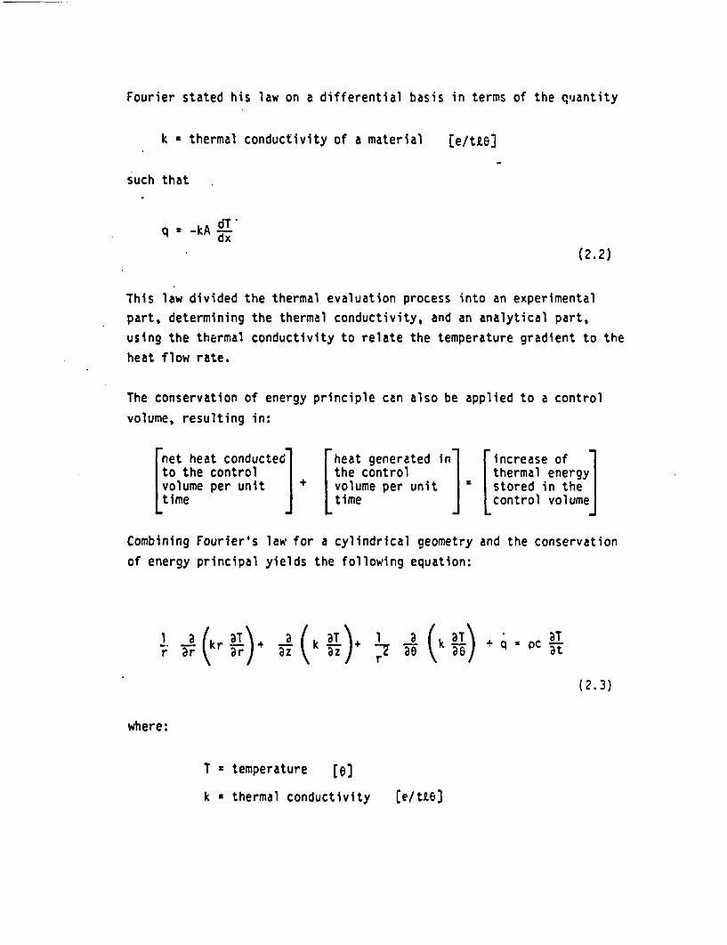
Fourier stated his law on a differential basis in terms of the quantity
k thermal conductivity of a material [e/ttel
such that
q -kA dT'dX(2.2)
This law divided the thermal evaluation process into an experimental
part, determining the thermal conductivity, and an analytical part,
using the thermal conductivity to relate the temperature gradient to the
heat flow rate.
The conservation of energy principle can also be applied to a control
volume, resulting in:
[ net heat conducte(to the controlvolume per unittime
d. heat generated inthe control
+ volume per unittime
_ increase ofthermal energy
. stored in the |_ L control volume
Combining Fourier's law for a cylindrical geometry
of energy principal yields the following equation:
and the conservation
r a r a) ^ k BT )+ I a k q aT
(2.3)
where:
T temperature [el
k thermal conductivity e/mtie
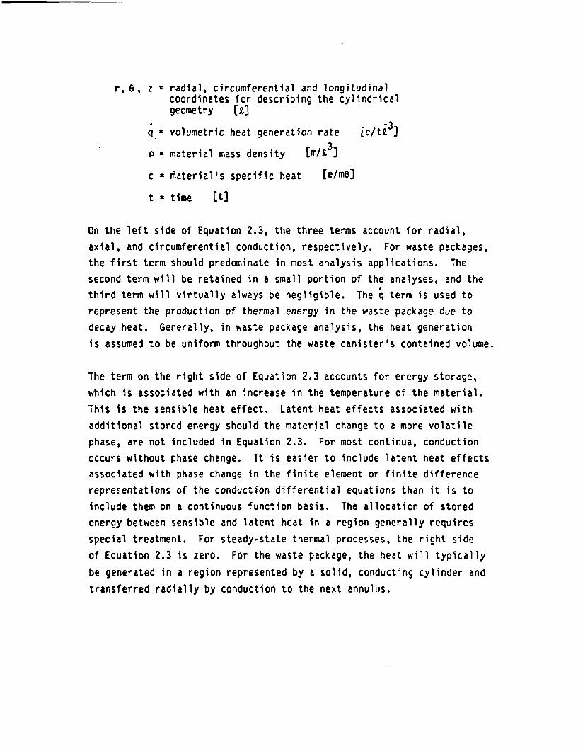
r, 6, z radial, circumferential and longitudinalcoordinates for describing the cylindricalgeometry [e.
-3q x volumetric heat generation rate [e/ti J
P material mass density fm/t3]
c = aterial's specific heat fe/me]
t time It]
On the left side of Equation 2.3, the three terms account for radial,
axial, and circumferential conduction, respectively. For waste packages,
the first term should predominate in most analysis applications. The
second term will be retained in a small portion of the analyses, and the
third term will virtually always be negligible. The term is used to
represent the production of thermal energy in the waste package due to
decay heat. Generally, in waste package analysis, the heat generation
is assumed to be uniform throughout the waste canister's contained volume.
The term on the right side of Equation 2.3 accounts for energy storage,
which is associated with an increase in the temperature of the material.
This is the sensible heat effect. Latent heat effects associated with
additional stored energy should the material change to a more volatile
phase, are not included in Equation 2.3. For most continua, conduction
occurs without phase change. It is easier to include latent heat effects
associated with phase change in the finite element or finite difference
representations of the conduction differential equations than it is to
include them on a continuous function basis. The allocation of stored
energy between sensible and latent heat in a region generally requires
special treatment. For steady-state thermal processes, the right side
of Equation 2.3 is zero. For the waste package, the heat will typically
be generated in a region represented by a solid, conducting cylinder and
transferred radially by conduction to the next annulus.
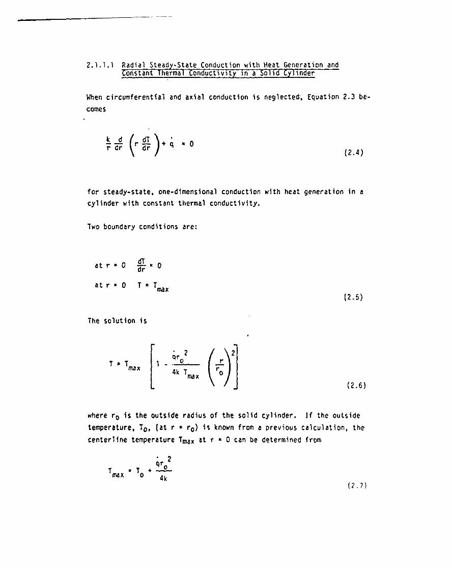
2.1.1.1 Radial Steady-State Conduction with Heat Generation andConstant Thermal Conductivity in a Solid Cylinder
When circumferential and axial conduction is neglected, Equation 2.3 be-
comes
k d (r dT ) q °r dr dr / + (2.4)
for steady-state, one-dimensional conduction with heat generation in a
cylinder with constant thermal conductivity.
Two boundary conditions are:
at r ° ddL - 0dr
at r T TX
(2.5)
The solution is
T s Tmax I'2or0
4k r0(-Y (2.6)
where r is the outside radius of the solid cylinder. If the outsidetemperature, To, (at r r) is known from a previous calculation, the
centerline temperature Tmax at r 0 0 can be determined from
Tru T + ro-IMx 0 4k(2.7)

2.1.1.2 Radial Steady-State Conduction without Heat Generationand with Constant Thermal Conductivity in a Hollow Cylinder
Equation 2.3 reduces to
r d U (r )
(2.8)
for radial steady-state conduction without heat generation and with
constant thermal conductivity in a region with inside radius ri and
outside radius r. Two boundary conditions are:
r r T To (To known)
r r dT 2iq tk (q, r, , k known)
(2.9)
The second
rate [e/tJ
annulus is
boundary condition is Fourier's law, and q is the heat flow
through the annular region. The heat generation within the
assumed to be zero.
The solution is
En (ro)
(2.10)
For waste package analysis, the temperature at the inside surface is
usually of interest and is given by
Ti T + ?% ktn r
(2.11)
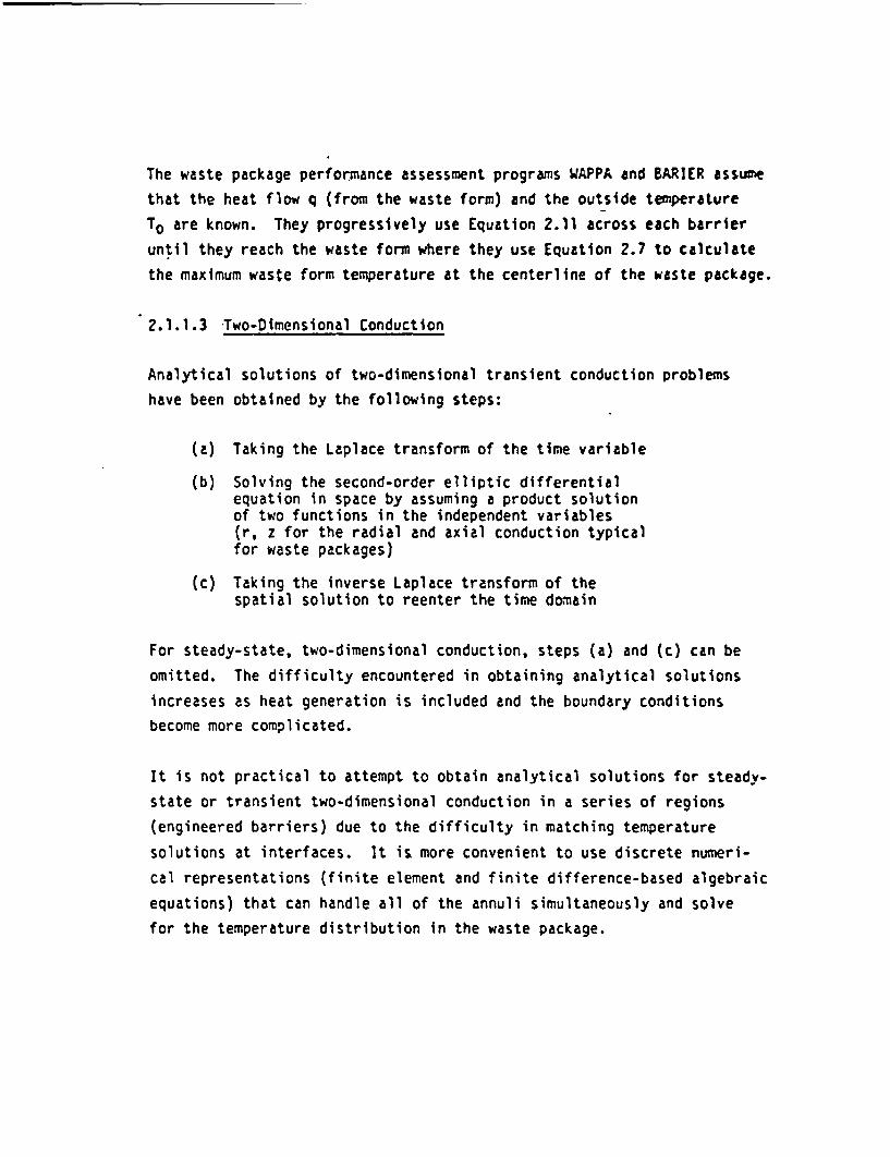
The waste package performance assessment programs WAPPA and BARIER assume
that the heat flow q (from the waste form) and the outside temperature
To are known. They progressively use Equation 2.11 across each barrier
until they reach the waste form where they use Equation 2.7 to calculate
the maximum waste form temperature at the centerline of the waste package.
2.1.1.3 Two-Dimensional Conduction
Analytical solutions of two-dimensional transient conduction problems
have been obtained by the following steps:
(a) Taking the Laplace transform of the time variable
(b) Solving the second-order elliptic differentialequation in space by assuming a product solutionof two functions in the independent variables(r, z for the radial and axial conduction typicalfor waste packages)
(c) Taking the inverse Laplace transform of thespatial solution to reenter the time domain
For steady-state, two-dimensional conduction, steps (a) and (c) can be
omitted. The difficulty encountered in obtaining analytical solutions
increases as heat generation is included and the boundary conditions
become more complicated.
It is not practical to attempt to obtain analytical solutions for steady-
state or transient two-dimensional conduction in a series of regions
(engineered barriers) due to the difficulty in matching temperature
solutions at interfaces. It ii more convenient to use discrete numeri-
cal representations (finite element and finite difference-based algebraic
equations) that can handle all of the annuli simultaneously and solve
for the temperature distribution in the waste package.

2.1.2 Convection
Convective heat transfer occurs in fluid-occupied regions when a solid
boundary and fluid are at different temperatures. This mode of heal
teansfer is driven by the mass transport of the flowing fluid. The
solid boundary and the flowing fluid act as two bodies exchanging heat
from the one at higher temperature to the one at lower temperature.
Heat transfer between a solid and a fluid involves a temperature gradi-
ent in the fluid near the wall. The region over which this gradient
extends is known as the thermal boundary layer or convective film. Out-
side this boundary layer, the fluid temperature remains at the undis-
turbed bulk fluid temperature. The temperature gradient in the boundary
layer is accompanied by a density gradient. For a quiescent fluid re-
gion, the density gradient is acted on by gravity, and the fluid tends
to flow, causing mass transfer and heat exchange from a hot wall to the
fluid or from the fluid to a cold wall. If the fluid flow past the hot
or cold surface is caused only by the density gradient induced by the
temperature gradient, the heat transfer is known as natural convection
or free convection. If the flow past the hot or cold surface is caused
by other means, such as momentum imparted to the fluid by a fan or pump,
the heat transfer is known as forced convection.
The basic equation for convective heat transfer was stated by Newton in
1701:
q = hA(Th - Tc)
(2.12)
where
q heat flow rate fe/t)
h convective heat transfer coefficient [e/ti2el
A area of heat transfer surface [2 J
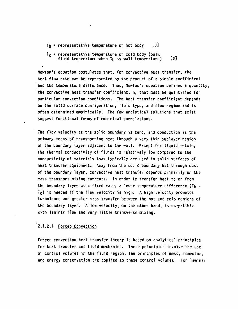
Th representative temperature of hot body [el
Tc representative temperature of cold body (bulkfluid temperature when Th is wall temperature) [6e
Newton's equation postulates that, for convective heat transfer, the
heat flow rate can be represented by the product of a single coefficient
and the temperature difference. Thus, Newton's equation defines a quantity,
the convective heat transfer coefficient, h, that must be quantified for
particular convection conditions. The heat transfer coefficient depends
on the solid surface configuration, fluid type, and flow regime and is
often determined empirically. The few analytical solutions that exist
suggest functional forms of empirical correlations.
The flow velocity at the solid boundary is zero, and conduction is the
primary means of transporting heat through a very thin sublayer region
of the boundary layer adjacent to the wall. Except for liquid metals,
the thermal conductivity of fluids is relatively low compared to the
conductivity of materials that typically are used in solid surfaces of
heat transfer equipment. Away from the solid boundary but through most
of the boundary layer, convective heat transfer depends primarily on the
mass transport mixing currents. In order to transfer heat to or from
the boundary layer at a fixed rate, a lower temperature difference (Th -
Tc) is needed if the flow velocity is high. A high velocity promotes
turbulence and greater mass transfer between the hot and cold regions of
the boundary layer. A low velocity, on the other hand, is compatible
with laminar flow and very little transverse mixing.
2.1.2.1 Forced Convection
Forced convection heat transfer theory is based on analytical principles
for heat transfer and fluid mechanics. These principles involve the use
of control volumes in the fluid region. The principles of mass, momentum,
and energy conservation are applied to these control volumes. For laminar

boundary layer flow in the x direction along a flat plate, as shown in
Figure 2.1, the mass conservation equation for incompressible, two-
dimensional, steady flow is
au a (
JZ.1 3)
where the two terms represent the fluid flow in the
the x and y directions and where
u local fluid velocity in the x direction
V local fluid velocity in the y direction
control volume in
[t)
[L/t]
The momentum conservation principle applied to laminar flow yields
uau YaU . a ax+ Ty y(2.14)
where
v :/p - fluid kinematic viscosity [u2 t)
j fluid dynamic viscosity Em/it]
P fluid mass density [m/ 33
xy coordinates as defined in Figure 2.1 [2.
and where the left side represents the net efflux of momentum from the
control volume due to exchanges of mass with the surroundings at differ-
ent velocities, and the right side represents the net viscous shear
force exerted on the fluid in the control volume.

y
flat plate in z-x plane
Figure 2.1
Control Volume in 1se Lominor Boundory Loyer an aFlat Plate

Applying the conservation of energy principle yields
DaT v T c2Tax+ Y v
(2.15)
where
T = fluid temperature at a point [6)
a = k/pc = fluid thermal diffusivity [t2/t
k * fluid thermal conductivity (e/tie)
c = fluid specific heat [e/me)
p fluid mass density [T/i3I
The terms on the left side of Equation 2.15 represent the net rate atwhich energy leaves the control volume due to fluid mass crossing its
boundaries at different temperatures and the right side represents net
thermal energy conducted into the control volume.
The momentum and energy differential equations are similar in that both
are parabolic, and for v a, the temperature and velocity distributions
are identical. From this observation, it follows that the transfer of
momentum is analogous to the transfer of heat within the laminar boundarylayer when the Prandtl number (Pr v/a) is unity. Moreover, for a
plate with a constant surface temperature Ts the momentum and energy
equation have physically and mathematically similar boundary conditions:
Boundary ConditionsMomentum Equation Energy Equation
y O v = Oy=O u O T - Ts z 0
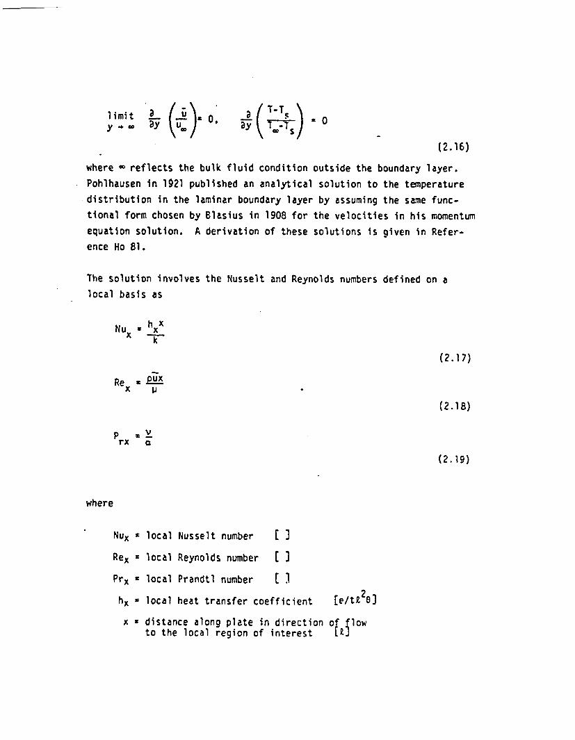
limit L ; 0,ym + o Y
a (T-T S)
(2.16)
where reflects the bulk fluid condition outside the boundary layer.
Pohlhausen in 1921 published an analytical solution to the temperature
distribution in the laminar boundary layer by assuming the same func-
tional form chosen by Blasius in 1908 for the velocities in his momentum
equation solution. A derivation of these solutions is given in Refer-
ence Ho 81.
The solution involves
local basis as
the Nusselt and Reynolds numbers defined on a
Nu X hXxk
(2.17)
Re . pux1Ij
(2.18)
P z vrx a
(2.19)
where
Nux local Nusselt number C I
Rex local Reynolds number I I
Prx local Prandtl number 3
h x local heat transfer coefficient [e/tt E
x distance along plate in direction of flowto the local region of interest CI
13

k fluid thermal conductivity Ce/tt6)
3P fluid mass density fm/ 3u fluid velocity in x direction parallel
to plate Cu/t]
V - dynamic viscosity of fluid [m/nt)
v.~ kinematic viscosity of fluid(v t /P) ft2/t]
thermal diffusivity of fluid tE2t)
The solution to the laminar thermal boundary layer equations is
Nux 0.332 Rexl/2 Prl/3.
(2.20)
Typically, it s more convenient to know the average Nusselt number over
a length of plate L
Nu hL7 'Fk(2.21)
where
L = length of plate in flow directionof interest for convection [t]
= average heat transfer coefficient overlength of plate L [e/tt2e)
so the associated average heat transfer coefficient can be evaluated.The average Nusselt number can be evaluated using
L
Nil i o O hxx
(2.22)

where hx, obtained from Equations 2.17, 2.18, and 2.20 is
T. 0.332 k 1/2112 p 1/3r
(2.23)
The solution to Equation 2.22 is then given by
Nu 0.664 ReL1/2 Prl/3
(2.24)
The associated average heat transfer coefficient for the length L of the
plate is
h 0.664(k/L)ReLl/ 2 Prl/3
(2.25)
when the flow in the boundary layer is laminar.
Analytical solutions have been determined for the laminar boundary layer
and for -le geometries. Experimentalists have assumed similar relation-
ships hold between the nondimensional quantities (Nu, Re, and Pr) such
that
Nu C Rem Prn
(2.26)
The values of C, m, and n can be evaluated for sets of laboratory data
to develop empirical correlations. Alternatively, the empirical process
has also suggested modifications in the functional forms that have been
used in correlating the Nusselt number and heat transfer coefficient.

2.1.2.2 Free or Natural Convection
Consider the.pane of glass shown in Figure 2.2, with an outside surface
temperature of 160C and an outside air bulk temperature of -180C. The
heated air moving upward next to the outside surface of the glass forms
a region of flow that is known as a boundary layer. At its inner edge,
the velocity is zero and the air temperature is equal to the temperature
of the glass pane's outer surface. Within the boundary layer, heat
transfer occurs primarily by conduction, but the overall transfer rate
process is treated as convection. At the outer edge of the boundary
layer, the temperature of the air is equal to the ambient air temperature
(bulk fluid temperature), and the velocity equals zero. This is true
because the air at rest at the edge of the boundary layer is not in a
forced flow condition and therefore cannot sustain any shear force. If
the temperature gradient were not zero at that point, heat would be
conducted out of the boundary layer causing an extended density gradient
and more upward flow.
The consequence of these temperature and velocity profiles is that no
heat flows from the glass through the boundary layer to the ambient air
(bulk fluid). All of the heat goes into the moving boundary layer which
has temperature and velocity profiles as depicted in Figure 2.3 and a
mean temperature intermediate to that of the glass pane and the ambient
air. Note that the temperature of the boundary layer, which is one of
the heat exchange media, is not used in Newton's equation. Rather, the
bulk temperature outside the boundary layer is used. The reason for
this choice is simply that the bulk fluid has a unique temperature value
while the boundary layer has an unquantified temperature distribution.
The same assumptions apply in the application of the mass and energy
conservation principles to natural convection as for forced convection,
yielding the same mathematical relationships. However, the momentum
conservation principle includes a net force resulting from the pressure
gradient and a gravitational force term which must be retained. For
forced convection they were neglected since they are much smaller than
the viscous force term. Thus, the equations resulting from the mass,
20

T = 160C
dy
L[3 dx
T= -18 Cucv:o
gloss inx-z plane
y
Figure 2.2
Nalurol Convection Bonxdory Layer Along OutsideSurface of a Worm Pone of Gloss in Cold Ambient Air
21

1 60C
.-. y
Figure 2.3
Velocity and Temperature Profilesin Natural Convection
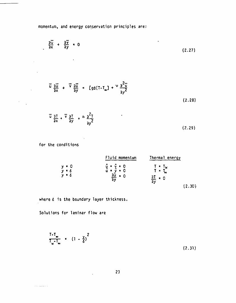
momentum, and energy conservation principles are:
au+ - v 0a X ay
(2.27)
u aax
+ v au ay CgB(T-T +
(2. 28)
u aT v aT a a2Tax ay Y2
(2. 29)
for the conditions
Fluid momentum Thermal energy
y s 0y 6y 6
u - v
auay
zQ0
=.00
T TwT T.
BT = Oay
(2.30)
where 6 is the boundary layer thickness.
Solutions for laminar flow are
T-T
w C(1 - Y26
(2.31)
23
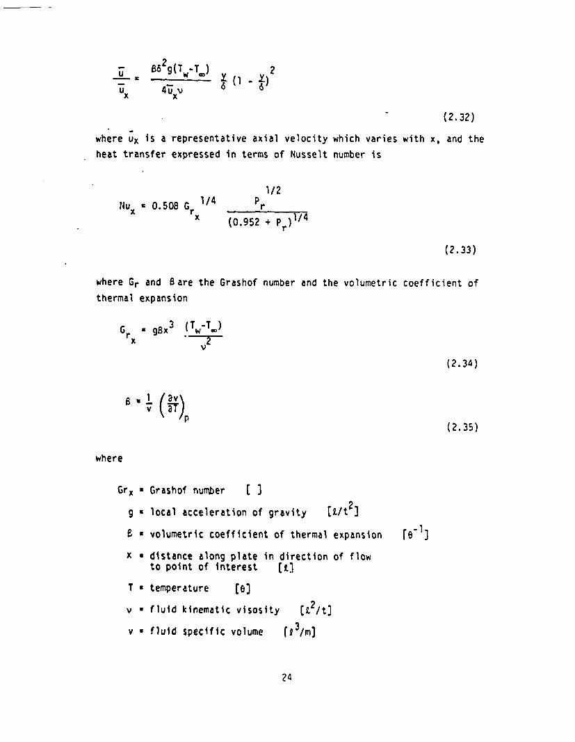
__ B62g(T -T ) -X2
4uv = ( - )
x~~~
(2.32)
where UX is a representative axial velocity which varies with x, and the
heat transfer expressed in terms of Nusselt number is
Nu 0.508 G 1 /4
1/2Pr
(0.952 + Pr )/
(2.33)
where Gr and Bare the Grashof number and the volumetric coefficient of
thermal expansion
Gr gx (Tw-TW)x 9(
(2.34)
v (e)
where
(2.35)
Girx Grashof number I I
g local acceleration of gravity I
B a volumetric coefficient of thermal
x u distance along plate in directionto point of interest [LI
T a temperature [el
v - fluid kinematic visosity (L2/t:
v a fluid specific volume [ 3/m)
2W~t
expansion
of flow
rel
I
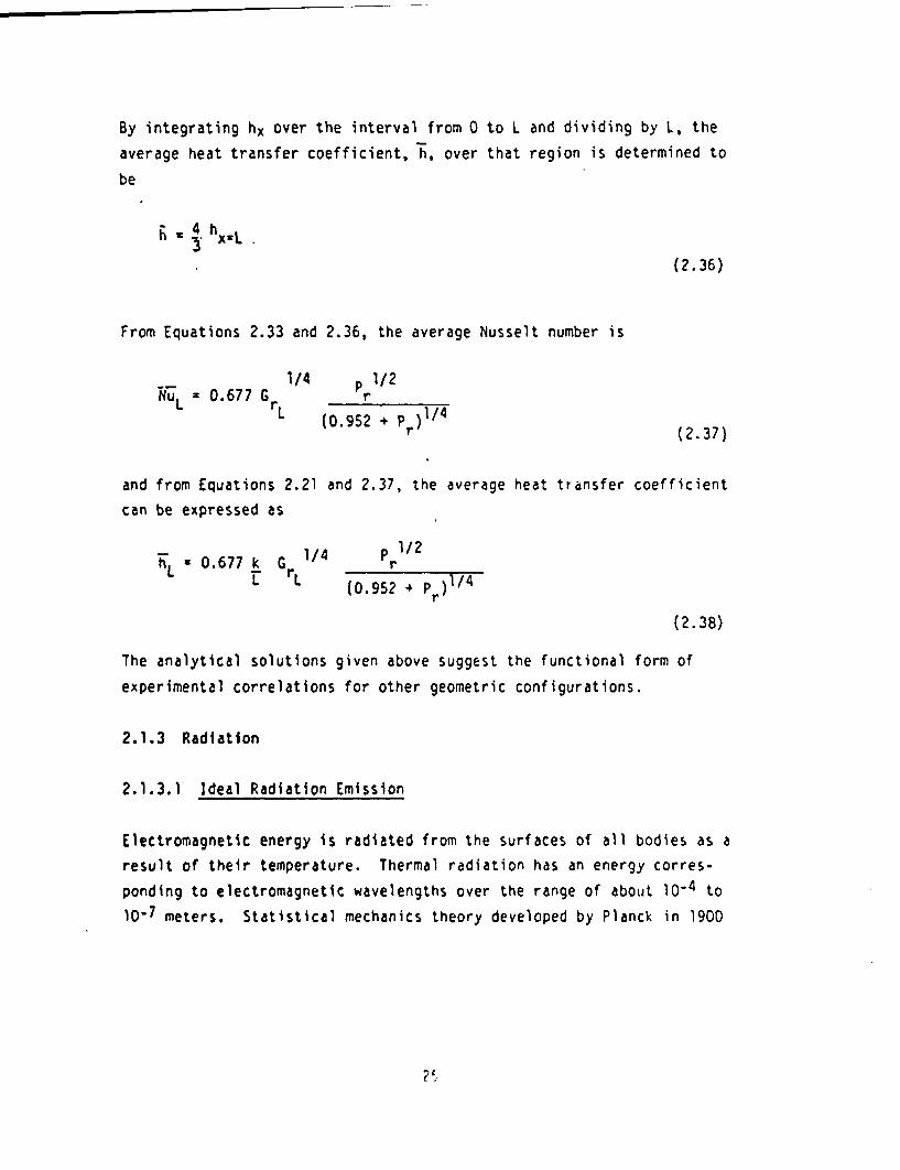
By integrating hx over the interval from 0 to L and dividing by L, the
average heat transfer coefficient, h, over that region is determined to
be
h . 4 hx-L (
(2.36)
From Equations 2.33 and 2.36, the average Nusselt number is
1/4WUL 0.677 GrL r~~~~~,
p 1/2r
IL (0.952 + P )1/4(2.37)
and from Equations 2.21 and 2.37, the average heat transfer coefficient
can be expressed as
WL 0.677 k G 1/4p 1/2
(0.952 P r)l/4
(2.38)
The analytical solutions given above suggest the functional form of
experimental correlations for other geometric configurations.
2.1.3 Radiation
2.1.3.1 Ideal Radiation Emission
Electromagnetic energy is radiated from the surfaces of all bodies as a
result of their temperature. Thermal radiation has an energy corres-
ponding to electromagnetic wavelengths over the range of about 104 to
10-7 meters. Statistical mechanics theory developed by Planck in 1900

yielded an expression for the energy density of radiation per unit
volume and per unit wavelength as a continuous function of the wave-length
8irhc)
P(WTr (2.39)
where
T temperature of body (OK) [e
h x Planck's constant 6.625 x 10⁻³⁴(J.sec) [et]
k a Boltzmann's constant 1.381 x 10⁻²³(J/molecule -OK) [e/molecule ]
c a velocity of light 3.0 x 10¹⁰ (cm/sec) (I/t)
A a radiant energy wavelength (cm) IQ)
- PA v radiant energy density per unit volujpeper unit wavelength (J/cm3) [e/L ]
In 1900, Boltzmann integrated this function over the spectrum from 0 toom
(all possible wavelengths) and determined the total radiant energy emittedby a body that will not transmit or reflect any incident radiation (a
black body) to be
Eb ' T4
(2.40)
where
Eb * total radiant thermal energy flux Ce/t2 I
c * Stefan-Boltzmann constant [e/t 264
T surface absolute temperature [el
2 ,
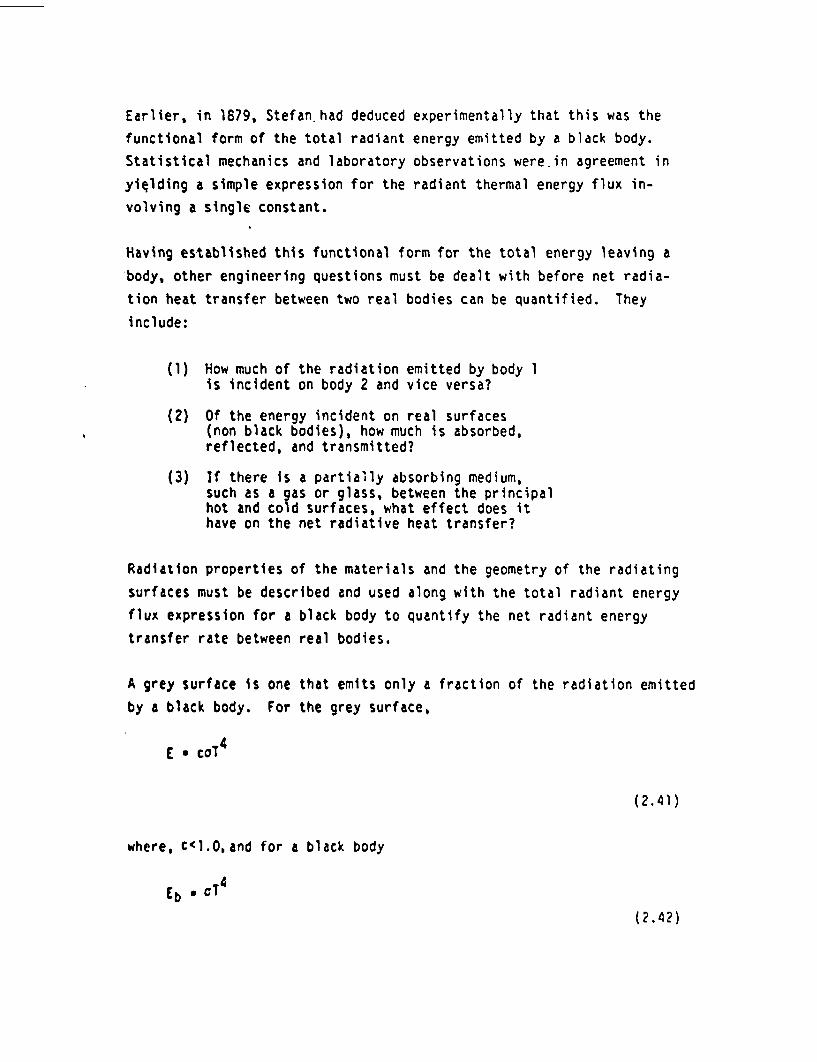
Earlier, in 1879, Stefan. had deduced experimentally that this was the
functional form of the total radiant energy emitted by a black body.
Statistical mechanics and laboratory observations were.in agreement in
yielding a simple expression for the radiant thermal energy flux in-
volving a single constant.
Having established this functional form for the total energy leaving a
body, other engineering questions must be dealt with before net radia-
tion heat transfer between two real bodies can be quantified. They
include:
(1) How much of the radiation emitted by body 1is incident on body 2 and vice versa?
(2) Of the energy incident on real surfaces(non black bodies), how much is absorbed,reflected, and transmitted?
(3) If there is a partially absorbing medium,such as a gas or glass, between the principalhot and cold surfaces, what effect does ithave on the net radiative heat transfer?
Radiation properties of the materials and the geometry of the radiating
surfaces must be described and used along with the total radiant energy
flux expression for a black body to quantify the net radiant energy
transfer rate between real bodies.
A grey surface is one that emits only a fraction of the radiation emitted
by a black body. For the grey surface,
E coT4
(2.41)
where, C.O, and for a black body
Eb . cT4
(2.42)
giving
EEb
(2.43)
The quantity is the emissivity and is a material surface property.
For a black body, c= 1 and for a grey body, 0 < C 1. For a grey body,
can be treated as a function of temperature. In some cases it is ac-
ceptable to consider as a constant.
If a black body, p, exchanges heat only by radiation and only with an-
other body at the same temperature,
ERate incident radiant energyn[is being absorbed by body p
CRate of energy loss byla L adiation from body p
OA EbA
(2.t44)
If the black body, p, is replaced with a grey body, q, at temperature
equilibrium, then
vAm' EA
(2.45)
where
* the radiation energy flux incident on either body [e/t )c a the absorbtivity of body p
Equations 2.44 and 2.45 -yield
rEb(2.46)
Equations 2.43 and 2.46 indicate
C &(2.47)
for all temperatures.
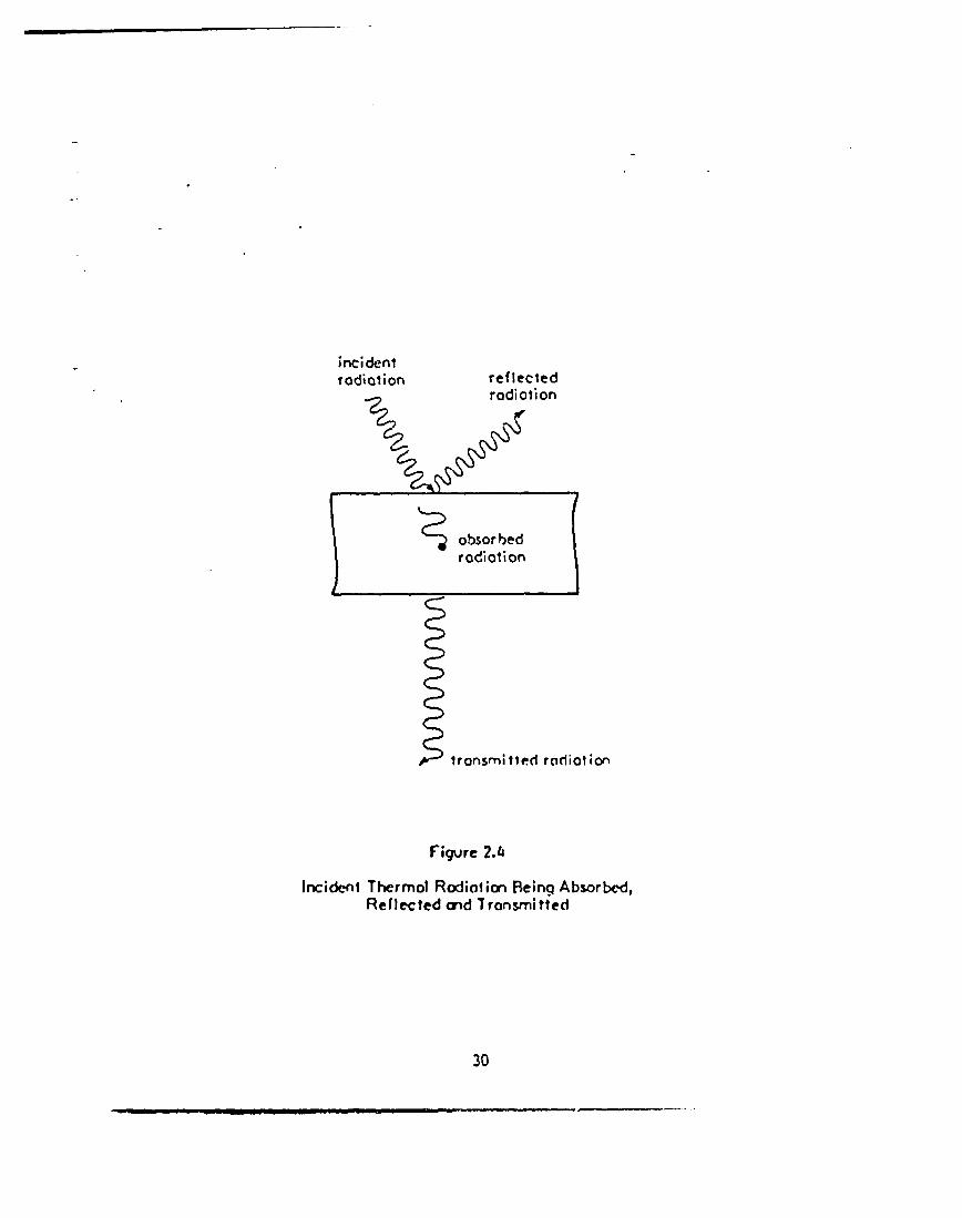
2.1.3.2 Material Radiation Properties
Of the total radiation incident on a ody, a fraction can be absorbed;another fraction reflected; and the remainder transmitted through the
body, indicated in Figure 2.4, such that
as P + T' 1(2.48)
where
I'* absorbtivity
o'is reflectivity
I I
[ II'df transmissivity
incidentrodiation reflected
radiation
Ironsmi led rdiol ion
Figure 2.4
Incident Thermol Radiaticn Pleinq Absorbed,Reflected and Tronsmitted
30
Most solid materials do-not transmit any thermal radiation so
CI + pa 1
in.those cases. For a black body P' T 0.
Energy that is reflected by or transmitted through a body maintains a
character (wavelength) associated with the temperature of the body from
which it was radiated. After energy has been absorbed by a body, future
radiation has a radiant energy flux which is related to the temperature
of that body.
2.1.3.3 Geometric Aspects of Radiative Heat Transfer
To quantify net radiative heat exchange, a "view factor" must be de-
termined. The view factor, Fn, is defined as the fraction of radiant
energy leaving the surface m that is incident on surface n. The view
factor is a nondimensional quantity ( Fmn' 1).
Consider two black bodies that exchange heat with one another. The net
heat transfer from body 1 to body 2 is
Q12 Ebl Al F12 - Eb2 A2 F21-(2.49)
When they are in temperature equilibrium with each other, (Tl T2), Q12
5 0, and Ebl = aT14 Eb2 T2
4 so that
Al F12 A2 F2 1
(2.50)
which is a reciprocity relationship. It applies in general to any two
surfaces (grey body or black body).

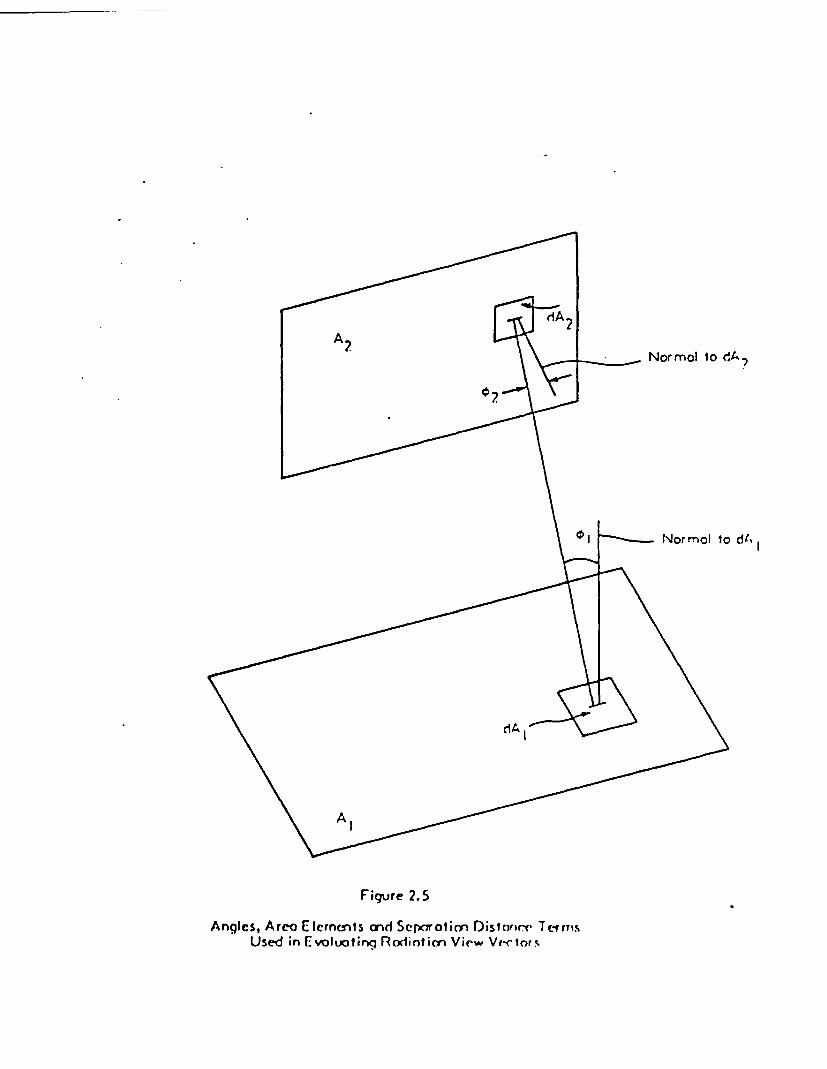
For the two black bodies shown in Figure 2.5, the net energy exchange
can be stated as
qnet (E E b2 os 2 cos At dA1 dA2
1-2 bl- b 2 .21
A2 A1 (2.51)
where hemispherical uniformity of radiation emission intensity is assumed,
and
Al 2 A2 2 21 T 7 cos 2 cos 0, dAl dA2
A A ~~~~~~~~~~(2.52)A2 A1
This result is convenient but not precisely accurate because the actual
intensity of the radiation emitted is generally non-uniformly rather
than uniformly distributed over a hemispherical surface as assumed in
the above equation.
2.1.3.4 Grey Body Radiation Heat Transfer
For grey bodies (< c a' <1) the radiation heat exchange is more com-
plex because part of the incident energy is always reflected from the
surface it reaches. The assumption of spatially uniform radiation in-
tensity from diffuse surfaces used previously for the black body heat
transfer description will be retained. To account for the net inter-
action between two bodies, it is convenient to define:
J radiation leaving a surface-radiosity [e/tk2]
G incident radiation on a surface-irradiation re/t2J
Assuming typical grey bodies which are opaque ( r's 0),
J - cEb +G
(2.53)
A;2Norrmol to dA ?
- Normnol lo dtI
A I
Figure 2.5
Angles, Area Elernomts Cnd Scprotin Disloor. Terr.Used in Evoluotinq Rod'ntian View Veclors

where the first term on the right side of Equation 2.53 accounts for
energy leaving the grey body, and the second term accounts for surface
reflection of incident radiation. Since a' + P 's 1, this can be written
as
J .cEb + (1-a')G(2.54)
The net energy leaving the surface is
q A(J-G) 3 A[cEb + (1-a')G - G]
q = A[cEb a -G]
(2.55)
Using Equation 2.54 in conjunction with Equations 2.55 and 2.47,
Eb J
(2.56)
This is an important relationship as it can be used in a manner analo-
gous to the use of Ohm's law to relate heat flow to potential difference
and resistance values. In this relationship q, which has units of
( e/t), is analogous to electrical current; Eb - J which has units of
e/tt23, is analogous to voltage difference; and (1-c)/cA, which has
units of CI/t2] , is analogous to electrical resistance.
Thus, for two grey bodies that see each other, a radiative heat transfer
network is
34
fbl .jl f b2
�bI .JI £p
f IA
Cray Body octor
I
ViewFoclor
I f 22 A 2
Gry Body Foctor
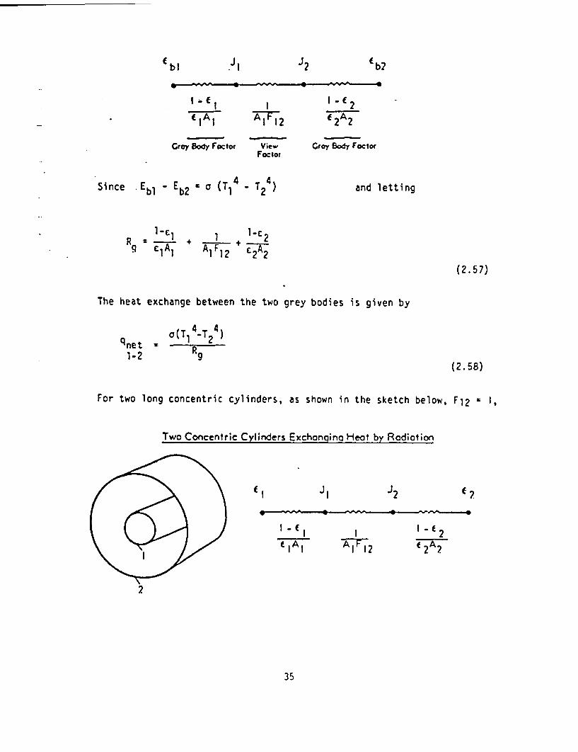
and lettingSince Ebt - Eb2 0 (T14 T2
4)
1 1Rg IAI F12
+ 2
(2. 57)
The heat exchange between the two grey bodies is given by
qnet1-2
a(T14-T2
4)
Rg
(2. 58)
For two long concentric cylinders, as shown in the sketch below, F12 1,
Two Concentric Cylinders Exchonaina Heot by Rodiation
JI f ,
-- . _0 -- - - -
I f I
f IA I IF1 2
f 2Ax
35
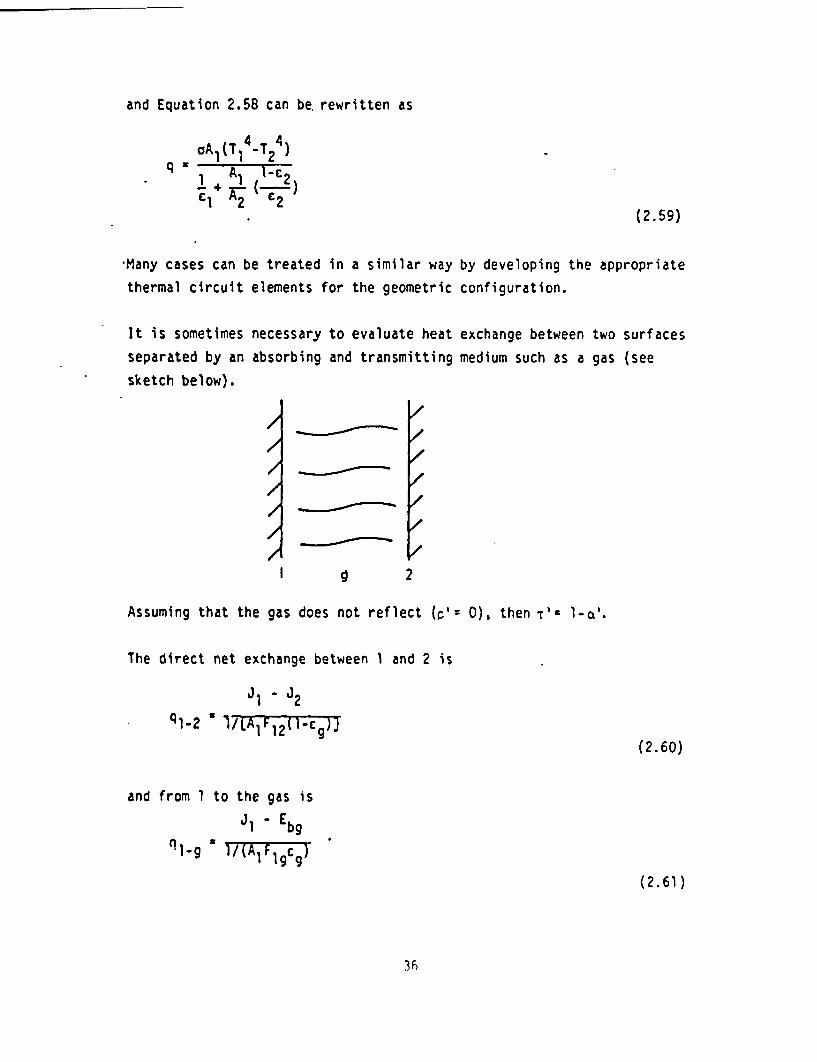
and Equation 2.58 can be. rewritten as
oA1(T1 -T2 )q 1 A1 2
cI 2 C(2.59)
'Many cases can be treated in a similar way
thermal circuit elements for the geometric
by developing the appropriate
configuration.
It is sometimes
separated by an
sketch below).
necessary to evaluate heat
absorbing and transmitting
exchange between
medium such as a
two surfaces
gas (see
I
/
////
/
V2
Assuming that the gas does not reflect (': 0), then I'd l-a'.
The direct net exchange between 1 and 2 is
qI-2~ J ' I/A q1-2 17LA112(1-C9)7
(2.60)
and from I to the gas is
J1 - Ebg
ql-g /(A IFlgcTT
(2.61)
3h

The radiation network becomes
f bg
AIFIgfg A2 29q Q
\ J2bI JI fb2
( 2 A2
I (I I
£IA1 AIF1 2 ' -cg).
It is usually easier to evaluate the overall resistance R between 1 and
2 after evaluating the individual resistances numerically rather than
functionally. For an equivalent network
R3 2 4
,bl / (b2
R5
with R, R2,
from surface
q1-2
R3, R4, and R evaluated numerically, the net heat radiated
1 to 2 is
o(T14 T24)
1 + R + RR 6
5 6(2.62)
where R6 R3 + R4.
17

2.1.4 Finite Increment Mathematical Models
The finite element and finite difference methods are used to analyze
complex heat transfer processes. These methods use a set of algebraic
equations to represent the energy conservation principle at discrete
intervals of time and space in place of continuous differential equa-
tions. The finite increment equations are written in terms of the
unknown temperature values at specified node locations. These equations
are coupled because each node temperature depends on that of its neigh-
boring nodes with which it directly interacts by exchanging heat. With
the finite increment method, a number of regions can be represented that
have different material property values, because properties such as
thermal conductivity, density, and specific heat are treated numerically.
This is a great advantage over continuous differential equations which
apply only in regions in which these parameters are continuous. For
multiple-regions the analytical effort required to solve the differential
equations when two-dimensional temperature variations are involved is so
great that this method becomes infeasible. Also, continuous differential
equations are much more difficult to solve if the properties are temperature-
dependent. With the finite increment methods, material property values
can be reevaluated after each solution based on the most recent local
temperature values.
The general form of the equations used in finite increment methods to
describe dynamic thermal equilibrium is
[ {T + [R] {Tt = {QX (2.63)
where [C] and [are the diagonal capacitance and generalized conduct-
ance matrices whose elements are determined from
Cii 6 i C V:(
(2.64)

ij tij j
ij (2.65)
where
6jj Kronecker delta 1 for i j and 0 i i
pi mass density of material associated with node i [W/t 3
Ci specific heat of material associated with node i Ce/mO]
V; tvolume of material associated with node i (
Cij ^ temperature specific energy capacity for node ifrom diagonal matrix [e/6]
kij thermal conductivity for conduction temperatureinteractions between nodes i and j [e/tte]
Axij a distance between nodes i and j [tQ
Ai heat transfer area for therial interactionbetween nodes i and j [IC]
Rij = thermal conductance between nodes i and j [e/te]
Qj - heat generation in the region associated withnode i from heat generation vector QI [e/t)
Ti s temperature at node i from vector ITI [e]
and where TI, TI, and Qlare the temperature vector for the assemblage
of nodes, the time derivative of the temperature vector and the vector
of heat generation rates associated with the various nodes, respectively.
This equilibrium relationship is formulated in many finite increment
programs by defining Kj differently in regions where convection is
occurring. This relationship may be expressed as
Kij hij Aij
(2.66)
) J

where
hij convective heat transfer coefficient appli ibleto exchange between nodes i and [e/ti e]
Similarly, radiation is frequently represented by an equation of form
identical. to Newton's equation
q hrA (Th - Tc)
(2.67)
where
q heat transfer rate [e/t)
hr equivalent radiative hal transfer coefficientfor radiation [e/ttc6j
Th = temperature of hot body surface [el
Tc temperature of cold body [e]
The heat transfer coefficient for radiation is defined as
hr o oF12 (Th2 + T 2)p (Th + T )p
(2.68)
where the subscript p indicates hr is evaluated based on the values of
Th and Tc in the previous iterations. When Equation 2.68 is multiplied
by the heat transfer area and the current temperature difference
(Th - Tc), the heat flow rate is determined. The thermal conductance
for finite increment models is determined from
Kij (hr)ij Aij
(2.69)
40

-
where
(hr)ij radiative heat transfer coefficient applicable 2to thermal radiation exchange between nodes i and j (e/ti e)
The dynamic thermal equilibrium equation has another term on the left
side when a phase change (assumed to be positive when going from a less
volatile phase I to a more volatile phase 2) is occurring. The equation
would be of the form
[c] hTI + R] TI + -IQ I
where
6ij i Vi hfg Ri liquid-gas
Ij
6ij Pi V hif Ri solid-liquid
(2.70)
where Pi and V are as previously defined and where
hfg = internal energy to gasify a unitmass of liquid [e/m
his internal energy to liq ify a unitmass of solid fe/mi
Ri - rate at which finite spatial regionassociated with node i is experiencingphase change [l/t)
Hi rate of energy increase causing phase changein spatial region associated with node i [e/t)
41

The quantities R are generally not specified directly. They may be
calculated on the basis of computer program algorithms that allocate
stored energy between sensible and latent heat. Phase-changes impose
the complication of different material properties for the two phases.
It is necessary to understand the procedures involved in various programs
that allow phase change as these procedures are not standardized.
2.1.5 Thermal Loads and Constraints
Thermal loads are typically specified in terms of a volumetric heat gen-
eration rate in a particular region of space. For a waste package, this
is likely to be a uniform heat generation rate for the inside of the
canister in its initial undeformed condition. The heat generation is a
consequence of the nuclear decay reactions. The parameters required for
the calculation of this decay heat generation as a function of time are
discussed in an earlier report in this series (Reference 1).
Two methods are commonly used for calculating the decay heat. The first
is a semi-empirical method which requires a knowledge of the fuel irradi-
ation history; the recoverable energy per fission of U235, Pu239, and
U238; and the number of fissions per initial fissible atom. The second
method is more detailed and case specific. It involves the use of a
depletion code like ORIGEN (Reference 2). In addition to the composition
of the fuel and its irradiation history, ORIGEN requires the input of the
following parameters: spectrum averaged cross sections; fission product
yields; radioactive decay constants, decay modes, and branching coeffi-
cients; radioactive chain decay information; and photon yields. Calcu-
lations are made to describe the decay heat rates for the actual waste
geometry and then re-expressed as a spatially uniform rate based on the
canister internal volume.
An important negative thermal load that must be considered in conjunction
with repository operation is the loss of heat associated with ventilation.
Ventilation will be required both for the initial burial of the waste and

its possible retrieval from the repository at a later time. The primary
mechanism for ventilation heat transfer is convection. The important
convection parameters such as the Reynolds number, Prandtl number, and
Nusselt number have been discussed in Section 2.1.2.1 of this report. If
significant temperature differences exist between different parts of a
repository, such as the waste package and repository walls, then the
convective heat loss terms must be corrected for thermal radiation ef-
fects. Heat loss from ventilation is discussed in an earlier report in
this series (Reference 3).
Thermal constraints are temperature conditions that the temperature dis-
tribution solution must satisfy. The temperature at various locations
can be fixed or specified as a function of time. Similarly, thermal
gradients can be specified at planes. Alternately, since the thermal
conductivity is generally known, the constraint can be specified as a
heat flux for the particular plane.
2.1.6 Conservation Equations
The conservation of energy principle applies throughout a conducting
medium. The finite element method applies the principle only at each of
the nodes used to describe the medium.
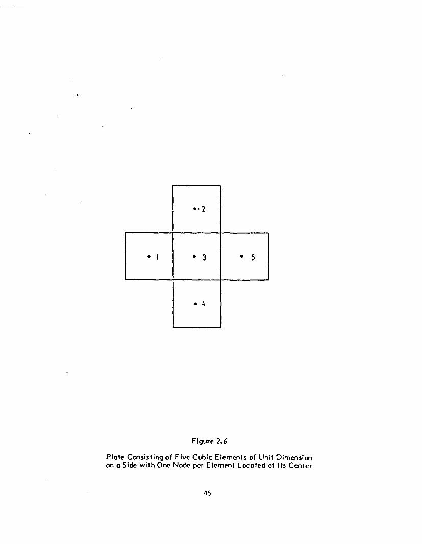
For conduction in the geometry shown in Figure 2.6, the energy conser-
vation principle applies to each of the five degrees of freedom - the
five nodes located at the center of the elements.
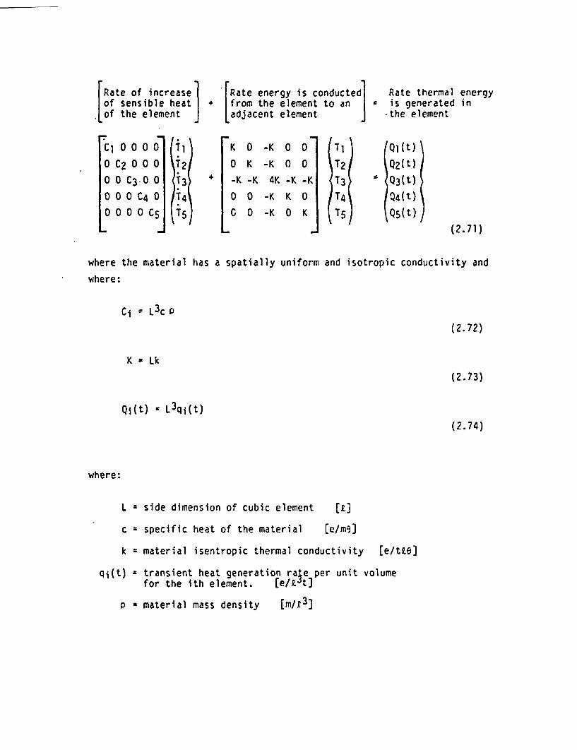
[Rate of increaseof sensible heat.of the element
0 C2 0 T2
0 0 C3.0 0 T3
0 0 0 C4 0 T4
0 0 0 0 C5 i5
[ Rate energy is conducted Rate thermal energy+ from the element to an I is generated in
adjacent element -the element
+
K 0 -K
O K -K
-K -K 4K
O 0 -K
0 0 -K
00
00
-K -K
KO
OK
T2
T3
T4
T5
Ql(t)
Q2 (t)Q3(t)
Q4(t)
Q5(t)(2.71)
where the material
where:
has a spatially uniform and isotropic conductivity and
Ci L3c
(2.72)
K Lk
(2.73)
Qi(t) L3qj(t)
(2.74)
where:
L = side dimension of cubic element [.E
c specific heat of the material le/m5)
k = material isentropic thermal conductivity [e/te]
qi(t) transient heat generation rale per unit volumefor the ith element. [e/I t]
P= material mass density [m/,3]
1 3 5
_ _
* 4
Figure 2.6
Plate Consisting of Five Ctic Elements of Unil Dimensionon a Side with One Node per Element Locoled ot Its Center

In matrix notation, the energy conservation equations become
[C) ITI + [K] IT = Q(t).
(2.75)
The quantities C and K can also be functions of time because they can
be re-evaluated (just as Q(t)) at the end of each time step at which
Equation 2.75 is solved. Equations 2.75 are sometimes known as the tempera-
ture equilibrium equations in that they represent the dynamic relationship
between temperature values and heat generation.
For steady state analyses, Equations 2.71 and 2.75 reduce to
K O
K
-K -K
0 0
0 0
-K 0 0
-K 0 0
4K -K -K
-K K 0
-K 0 K
Tl
T2T3T4
T5
Q1
Q 2Q3
Q4
Q5
41 4
(2.76)
and
[ ] ITI M IO :
(2.77)
Various elements used in the finite element method are defined in terms
of several nodes. Procedures contained in the computer software allocate
portions of the element properties such as volume, area, etc., to each
node.
Equation 2.77 can be solved by matrix methods. The general matrix
Equation 2.75 can be solved by direct integration, starting with some
known initial state of the system.
46

After the temperature distribution has been determined consistent with
the particular temperature boundary and initial conditions, the solution
can be checked at each node using the individual equations of Equation
2.75. These equations are no longer coupled since the temperature values
have been determined. The purpose of the check is to determine whether
thermal equilibrium exists, that is, does the left side of Equation 2.75
equal the-right within an acceptable tolerance at each node? The equi-
librium check need not be performed after each solution to Equation 2.75.
If the equilibrium check is not satisfied, the temperature distribution
should be modified and the check re-performed until satisfied.
2.1.7 Simulated Thermal Responses
When sufficient boundary conditions are applied (along with initial con-
ditions for transients), a unique spatial temperature distribution can be
obtained as the solution to Equations 2.75. This temperature distribution
is the fundamental response of a thermal analysis. From the temperature
distribution, gradients and heat fluxes can be calculated for various
planes. From these temperatures, the sensible heat storage and heat
conduction can be evaluated.
2.2 Thermal System Variables and Parameters
This section of the report presents a collection of data that will quan-
tify the physical properties of the thermal system that affect the con-
duction, convection, and radiation thermal energy transfer. These data
are provided here to aid waste package performance analysts by reducing
the effort involved in analytical modeling of the waste package physical
characteristics. The following materials are considered:
Cast iron
Low carbon steel
Stainless steel
Zircaloy
47
Titanium alloy.- Ticode-12
* High-level waste glass
• Uranium dioxide
• Bentonite
* Air
• Helium
H20 - liquid
* H20 - steam
These data were compiled during an investigation of limited scope and
are not always completely defined over the expected range of interest
for waste package design. Analysts may need to augment the data pre-
sented here with their own investigations in various areas, particularly
if material compositions differ from those chosen for the data summaries
in this report. The data are taken from published sources believed to
be reliable. The data are empirical, and different observers disagree
with regard to quantifying various physical parameters. For example, in
1967 an international conference presented more complete steam (and
liquid) properties for H20. Much attention was devoted to differences
that stemmed from different observations, which were probably the result
of both imprecise observation techniques and differences in the design
and control of the experiment.
2.2.1 Conduction Parameters
Three independent quantities must be defined in order to perform conduction
analyses. They are:
k - thermal conductivity [e/tZ6]
c - specific heat [e/mo)
o - mass density (rm/ 3)
48

Thermal diffusivity depends on the values of these three independent
quantities:
a =k = thermal diffusivity [ t]
(2.78)
Another independent quantity that needs to be defined for materials that
could experience phase change in the temperature range from 0 to 3000C
is the latent heat:
hf = latent heat [elm]
This quantity, expressed on a per unit mass basis, is of interest only
for H20. For steady-state conduction, specific heat and mass density
are not of interest as they appear only in the sensible heat storage
term, which is proportional to the time rate of change of temperature.
The thermal conductivity of gases is dependent on their pressure and
temperature. For liquids and solids, the thermal conductivity is de-
pendent on the material temperature. In some cases, this dependency can
be neglected and the conductivity considered as constant. For example,
if a steady-state state analysis is being performed in which the tempera-
tures can be estimated to within 250C, it is usually acceptable when
dealing with solids to treat the thermal conductivity values as constants
evaluated at the estimated average temperature.
.2.2.1.1 Thermal Conductivity
Thermal conduction is the flow of thermal energy from one region at a
high temperature to n adjoining region at a lower temperature. It is a
result of energy transferred through a substance by its free electron
migration and kinetic energy exchange due to molecular collisions in
which the molecules have vibrational kinetic energies proportional to
their temperature. Fourier's law provides a functional definition of
49
thermal conductivity of a substance by relating it to other observable
quantities:
q -kA TdX(2.79)
and
(2.80)
where
0 = heat flux [e/t 2
q = heat transfer rate [[e/t]
A = heat transfer area [.2 )
k thermal conductivity [e/tLS)
T temperature [el
x = distance along heat transfer direction Es]
The SI unit for thermal conductivity is watt per meter degree celsius,
W/(m-OC). Conversions for thermal conductivity units are:
1 cal/(cm-s-OC) 418.68 W/(m-OC)
I cal/(cm-s-OC) 241.9 Btu/(hr-ft-OF)
1 tu/(hr-ft-OF) 1.731 W/(m-OC)
1.Btu/(hr-ft-0F) 0.2162 (lbf/sec-OF)
2.2.1.2 !specific Heat
Sensible heat manifests itself inside a material as the sum of molecular,
kinetic, and potential energies. The sensible heat term describes stored
50
energy in terms of temporal change in temperature of a material's mass:
Qs PC ET
where
Q~S increase in stored energy in the formof sensible heat [e/tt3]
(2.81)
P material mass density
C
T
- material specific heat
- material temperature
[m/]
Ce/mO]
t time t].
This sensible heat term appears in the general (transient) conduction
equation developed from the energy conservation principle. The specific
heat is the thermal energy addition to a unit mass of material necessary
to raise its temperature by one degree.
For finite element and finite difference programs, it is frequently
advantageous to deal with the energy storage on a unit volume basis
rather than a unit mass basis. This is done by replacing the specific
heat (c) with the product of the specific heat and the mass density:
C '1 DC
(2.82)
The sensible heat storage term becomes
A dTQsS C F
(2. 83)
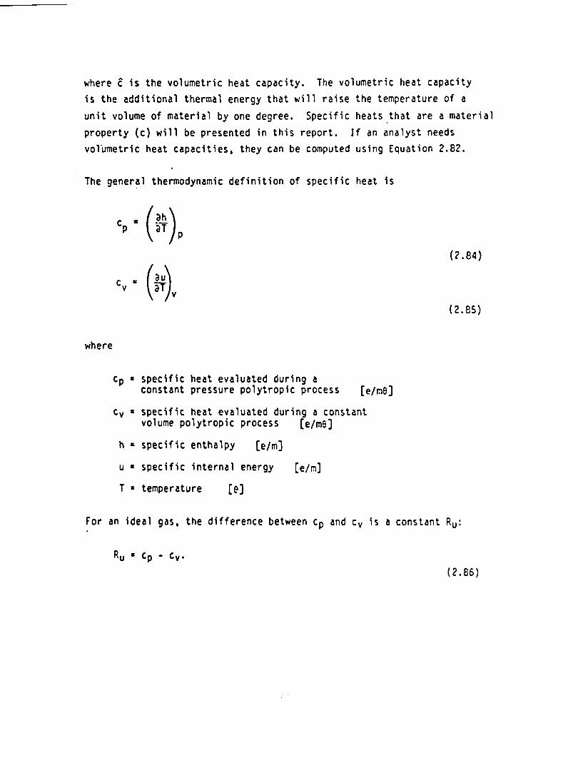
where c' is the volumetric heat capacity. The volumetric heat capacity
is the additional thermal energy that will raise the temperature of a
unit volume of material by one degree. Specific heats that are a material
property (c) will be presented in this report. If an analyst needs
volumetric heat capacities, they can be computed using Equation 2.82.
The general thermodynamic definition of specific heat is
kps (a)p
(2.84)
cv (uv
(2.85)
where
cp specific heat evaluated during aconstant pressure polytropic process [e/ne]
cv - specific heat evaluated during a constantvolume polytropic process [e/m53
h specific enthalpy [e/m)
u specific internal energy [e/m]
T temperature [e)
For an ideal gas, the difference between cp and cv is a constant Ru:
Ru Cp - Cv.
(2.86)
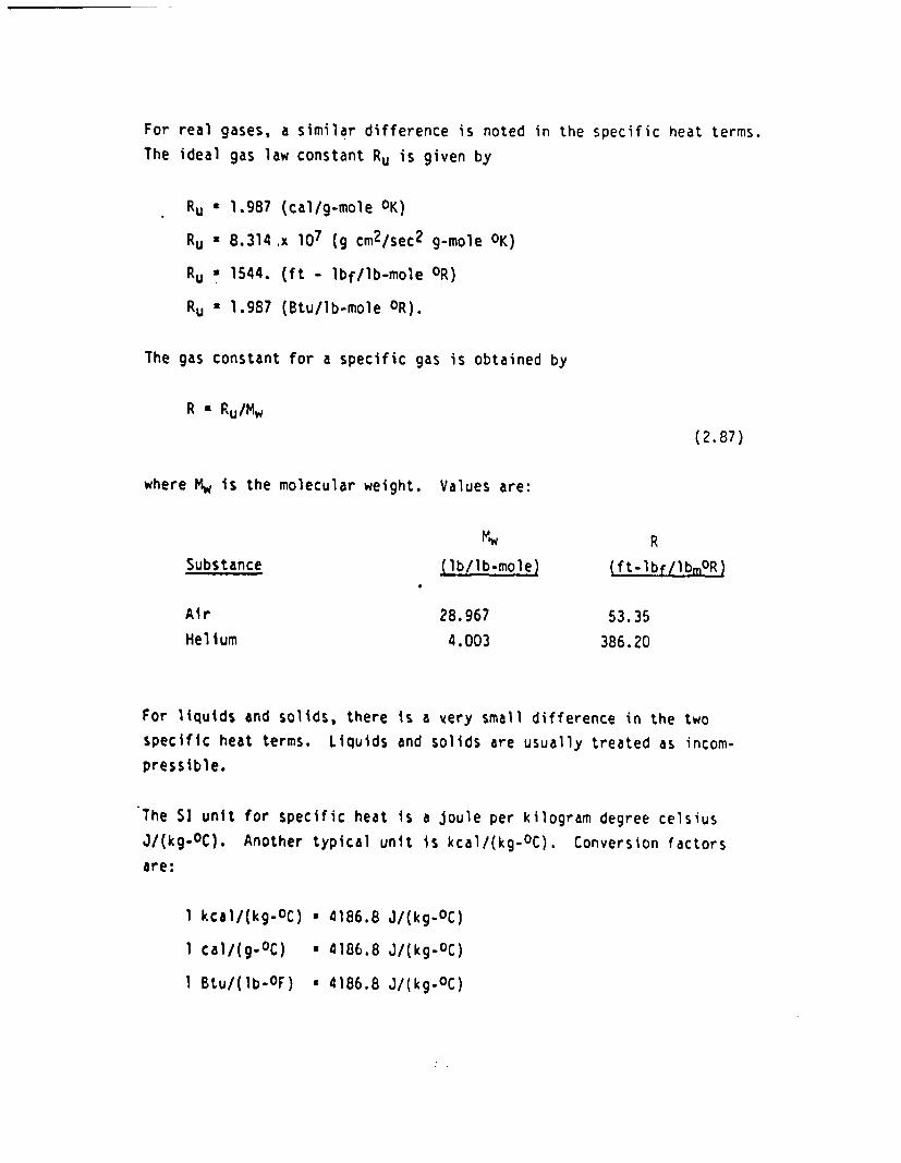
For real gases, a similar difference is noted in the specific heat terms.
The ideal gas law constant Ru is given by
Ru 1.987 (cal/g-mole OK)
Ru x 8.314 .x 107 (g cm2/sec2 -mole OK)
Ru a 1544. (ft - lbf/lb-mole OR)
Ru ' 1.987 (Btu/lb-mole OR).
The gas constant for a specific gas is obtained by
R Ru/Mw
(2.87)
where Mw is the molecular weight. Values are:
Substance (lb/lb-mole)
R
(ft-lbf/bmQR)
53.35
386.20
Air
Helium
28. 967
4.003
For liquids and solids, there
specific heat terms. Liquids
pressible.
is a very small difference in the two
and solids are usually treated as incom-
The SI unit for specific heat is a joule per kilogram degree celsius
J/(kg-OC). Another typical unit is kcal/(kg-OC). Conversion factors
are:
1 kcal/(kg-0C) 4186.8 J/(kg-OC)
1 al/(g.OC) * 4186.8 J/(kg-OC)
1 Btu/(lb-OF) * 4186.8 J/(kg-OC)
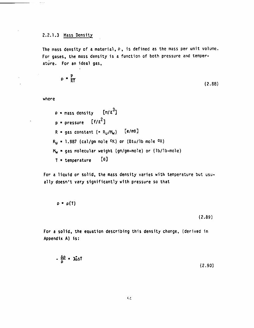
2.2.1.3 Mass Density
The mass density of a material, P, is defined as the mass per unit volume.For gases, the mass density is a function of both pressure and temper-ature. For an ideal gas,
p
(2.88)
where
0 mass density m/t 33
p pressure [f/t ]
R * gas constant ( Ru/Mw) [e/me)
Ru 1.987 (cal/gm mole OK) or (Btu/lb mole OR)
Mw gas molecular weight (gm/gm-mole) or (lb/lb-mole)
T * temperature [el
For a liquid or solid, the mass density varies with temperature but usu-
ally doesn't vary significantly with pressure so that
D ' (T)
(2.89)
For a solid, the equation describing this density change, (derived in
Appendix A) is:
- h 3A T (.9
(2. 90)
C e

For liquids, the data are usually tabulated in terms of either the mass
density or the specific volume versus temperature at fixed values of
pressure.
For virtually all substances, the mass density increases with decreases
in temperature. For gases, the mass density also increases with increasing
pressure;
The specific volume of a substance is the volume required to contain a
unit mass of the material at a given thermodynamic state, such as uniform
temperature and pressure. The specific volume is the reciprocal of the
mass density:
v
(2.91)
where
v specific volume t3,m]
p = mass density [m/t3]
Thus, only one of these two properties needs to be known.
When a substance is heated and is free to expand, it experiences a thermal
strain,
dc - dT(2.92)
without experiencing any stress. Over limited ranges of temperature
change, the elongation of a specimen can be described by
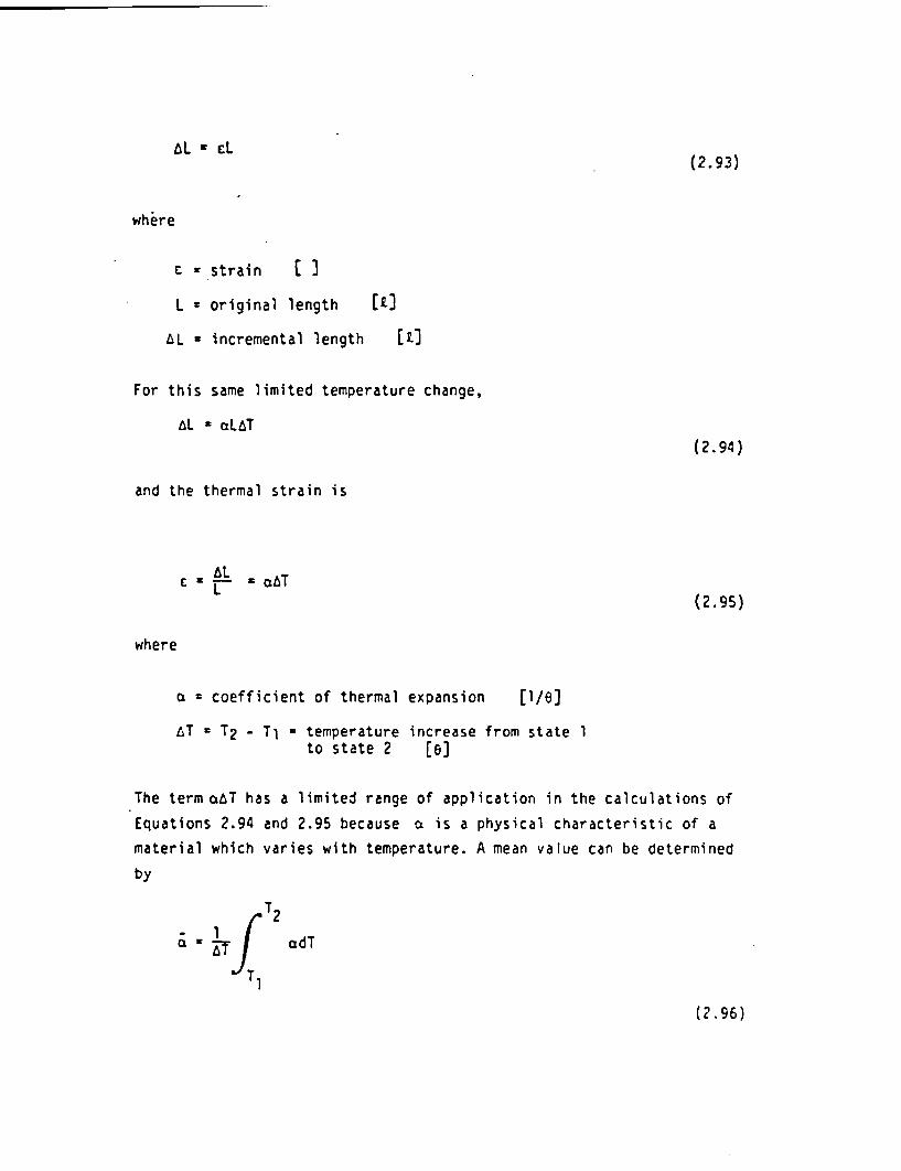
AL EL(2.93)
where
E = strain
L = original length [El
LL = incremental length Liz
For this same limited temperature change,
aL cLtT(2. 94)
and the thermal strain is
c = LL = W
(2.95)
where
a = coefficient of thermal expansion [1/el
LT T2 - T temperature increase from state 1to state 2 [o6
The term abT has a limited range of application in the calculations ofEquations 2.94 and 2.95 because is a physical characteristic of a
material which varies with temperature. A mean value can be determined
by
f T2
a 0 ,, adT
(2.96)

where
z mean coefficient of thermal expansionover the range Tl. T < T2.
When the temperature of a substance is increased the substance experi-
ences a fractional volume change according to
b 3&eT (2.97)
and for constant mass
V ((7.98)
so that the fractional change in mass density is
- AP - 3T
(2.99)
whEre
a = mean coefficient of thermal expansion [1/e]
ET = temperature increase [el
These relationships are developed in Appendix A. They can be used to
determine approximately how the mass density varies with temperature for
a solid when the thermal expansion coefficient data are known.
The SI unit for mass density is g/m3. Other typical units are kg/m3 and
ibm/ft3. Conversion factors are:
1 k/m3. 1000 g/m3
1 kg/m3 0.0624 bm/ft3
Since specific volume is the inverse of mass density, these conversion
factors can be used for specific volume.
2.2.1.4 Latent Heat
Within a heat transfer region, a phase change can occur when the pres-
sure and temperature have a particular combination of values so that two
phases of a substance coexist in equilibrium. The heat transfer can
continue without temperature change and with the material changing phase
either giving up energy when going to a less volatile phase or absorbing
energy when going to a more volatile phase.
Latent heat derives its name from the fact that the internal energy of a
substance can change without a change of temperature. This occurs when
a material gradually changes phase with a step function difference in
internal energies between the two phases.
The science of calorimetry, which preceded the development of the thermo-
dynamic laws, devised the concept of latent heat. This early work involved
important physical observations, but some were not stated as precisely
as needed for consistency with the thermodynamic laws and principles
which were developed later. The early definition of latent heat was:
"Latent heat is the amount of heat which must be added to a unit mass of
a substance to cause it to change phase in a constant pressure, constant
temperature, frictionless process." The definition is expressed as
follows:
Q mqL mau + W
(2.100)
I ,.
where
Q total heat added [e]
m z mass of substance changing phase [m]
qL = latent'heat per unit mass e/m]
Au z.change in specific internal energy of material [elm]
W work done by volume change by the entire systemof mass m without friction fe]
Latent heat can also be defined as a material property rather than heat
flow during a process. For an open system, the stream flowing into the
system can do work on the system, and the stream flowing out of the
system can have work done on it by the system.
The work in either stream is
w FL pAL = pV
(2.101)
where
w = flow work per unit time [e/t]
F total force exerted on the quantityof fluid flowing across boundary(inlet or outlet) per unit time [f/t]
L length of unit mass of fluid flowingacross boundary in unit time [2.]
p pressure at inlet (or outlet) [U/t 2
A area of flow into or out of system [k2)
V - volume of fluid flowing across boundaryin unit time f13/tj
Equation 2.101 can be written on a per unit mass basis
w pv
(2.102)
where
v specific volume of fluid crossing boundary [L 3/m].
w work per unit mass e/rm]
Pressure and specific volume are properties of the fluid. Thus, the
flow work is a property of the fluid. The enthalpy is a fluid property
defined as
h u pv
(2.103)
where
h = specific enthalpy per unit mass [e/m)
u specific internal energy per unit massWZ2 I
[e/m]
p = pressure
(13/m]v = specific volume
Latent heat is defined as the difference between the specific enthalpy
of one phase of a pure substance at saturation conditions and the spe-
cific enthalpy of another phase of the pure substance at the same pres-
sure and temperature.
The latent heat terms are
hf = h - hf [2](2.104)
60

hif Uhf - hfm ],
(2.105)
hjg h9 -h
(2.106)
where 9, f, and i represent the gas, liquid, and solid phases. Equa-
tions 2.104, 2.105, and 2.106 represent the latent heat associated with
liquid-gas, solid-liquid, and solid-gas transformations respectively.
2.2.1.5 Paterial Conduction Properties
Tables in this section present the conduction properties, thermal conduc-
tivity (k), mass density (), specific heat (c), and thermal diffusivity
(a), for each of the following solid materials:
* Cast iron (Tables 2.1 and 2.2)
* Carbon steel (Tables 2.3 and 2.4)
• 304 stainless steel (Tables 2.5 and 2.6)
* Ticode 12 (Tables 2.7 and 2.8)
• Zircaloy 2 (Tables 2.9 and 2.10)
* Zircaloy 4 (Tables 2.11 and 2.12)
* Bentonite (Tables 2.13 and 2.14)
• High-level waste glass (Tables 2.15, 2.16, 2.17, and 2.18)
* Uranium dioxide (Tables 2.19 and 2.20)
These same properties are also presented as a function of pressure and
temperature for air and helium at low pressure, saturated liquid water,
and dry saturated steam (Tables 2.21 - 2.28). For water and steam,
saturation properties including specific volume (reciprocal of mass
density) and specific enthalpy are presented in Tables 2.29 and 2.30.
Thermal conductivity, specific volume, and specific enthalpy are pre-
sented in Tables 2.31 - 2.36 as a function of pressure and temperature
for
* Subcooled liquid water
a Superheated steam
* Saturated water
* Saturated steam

Table 2.1
Cast Iron Conduction PropertiesIncluding Thermal Conductivity (k), Mass Density (),Specific Heat (cp), and Thermal Diffusivity (a = k/Pc)
in English Units
T(OF)
32
212
572
932
k(Btu/hr-ft-OF)
33.0
31.8
27.7
24.8
(lbm/ft3) (Btu/9M°F)
474
472
469
466
0.110
0.110
0.110
0.110
a(ft2/hr)
0.633
0.612
0.537
0.483
.r
-I
Source: KR-61 (k,Cp)
Ma-78 (P)
a * K/OCp
-J
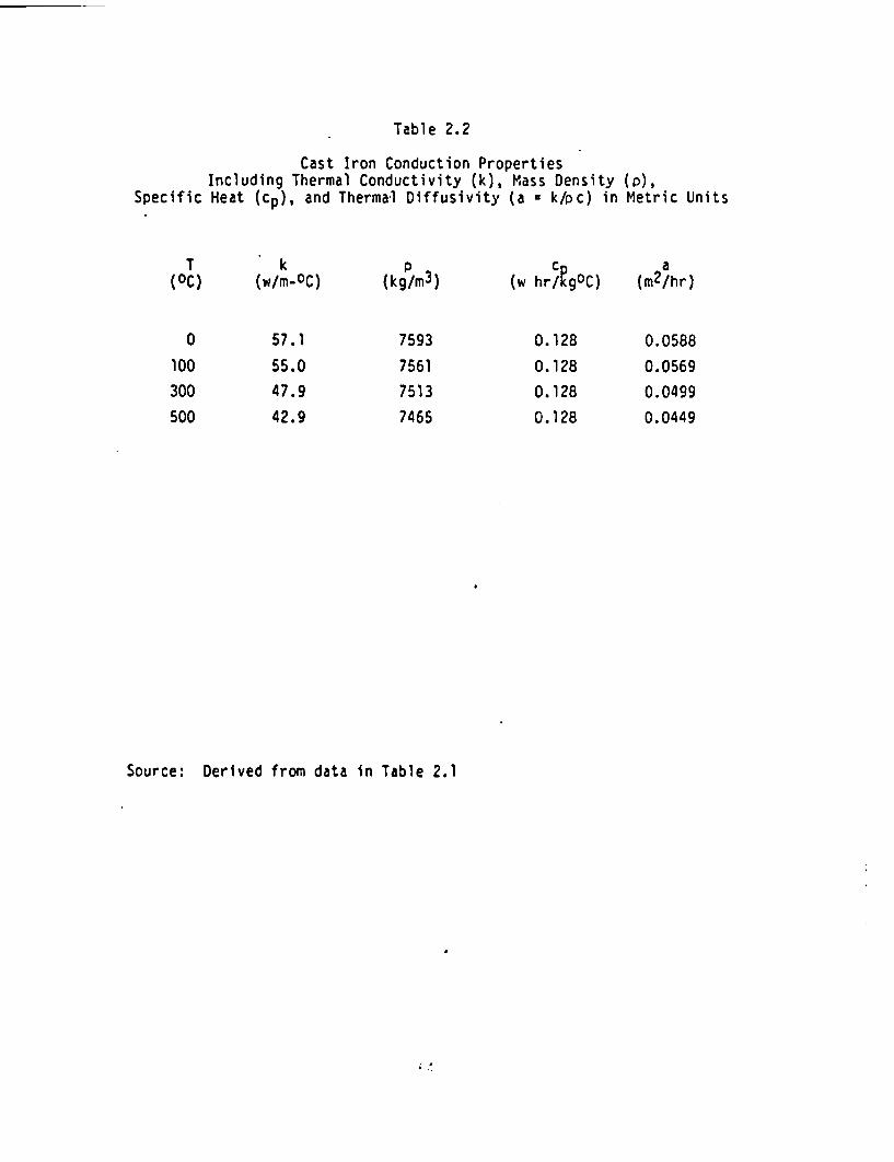
Table 2.2
Cast Iron Conduction PropertiesIncluding Thermal Conductivity (k), Mass Density
Specific Heat (cp), and Thermal Diffusivity (a k/pc) in(P),Metric Units
T(0C)
0
100
300
500
k(w/m-OC)
57.1
55.0
47.9
42.9
(kg/rm 3 )
7593
7561
7513
7465
(w hr/kgOC) (m2/hr)
0.128
0.128
0.128
0.128
0.0588
0.0569
0.0499
0.0449
Source: Derived from data in Table 2.1
; A*
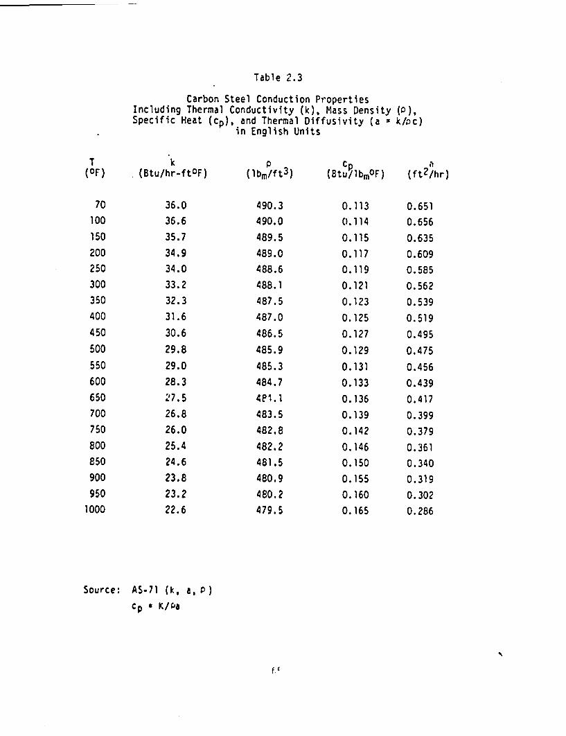
Table 2.3
Carbon Steel Conduction PropertiesIncluding Thermal Conductivity (k), Mass Density (),Specific Heat (cp), and Thermal Diffusivity (a k/oc)
in English Units
(OF)
70
100
150
200
250
300
350
400
450
500
550
600
650
700
750
800
850
900
950
1000
k(Btu/hr-ftOF)
36.0
36.6
35.7
34.9
34.0
33.2
32.3
31.6
30.6
29.8
29.0
28.3
;7.5
26.8
26.0
25.4
24.6
23.8
23.2
22.6
(lbm/ft 3 )
490.3
490.0
489.5
489.0
488.6
488.1
487.5
487.0
486.5
485.9
485.3
484.7
483.5
482.8
482.2
481.5
480.9
480.2
479.5
(Btu/lbmOF)
0.113
0.114
0.115
0.117
0.119
0.121
0.123
0.125
0.127
0.129
0.131
0.133
0.136
0.139
0.142
0.146
0.150
0.155
0.160
0. 165
(ft 2 /hr)
0.651
0.656
0.635
0.609
0.585
0.562
0.539
0.519
0.495
0.475
0.456
0.439
0.417
0.399
0.379
0.361
0.340
0.319
0.302
0.286
Source: AS-71 (k, a, )
cp K/fD
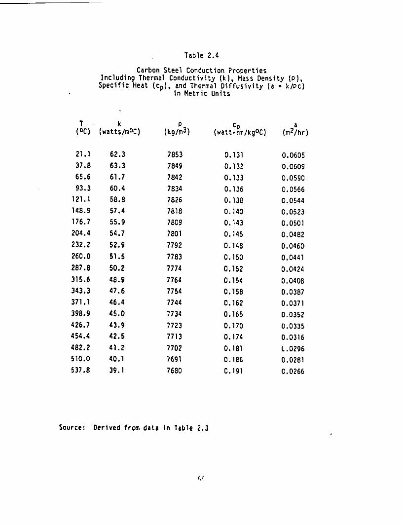
-
Table 2.4
Carbon Steel Conduction PropertiesIncluding Thermal Conductivity (k), Mass Density (),Specific Heat (cp), and Thermal Diffusivity (a k/Pc)
in Metric Units
T k(OC) (watts/mOC)
21.1
37.8
65.6
93.3
121.1
148.9
176.7
204.4
232.2
260.0
287.8
315.6
343.3
371.1
398.9
426.7
454.4
482.2
510.0
537.8
62.3
63.3
61.7
60.4
58.8
57.4
55.9
54.7
52.9
51.5
50.2
48.9
47.6
46.4
45.0
43.9
42.5
41.2
40.1
39.1
p(kg/m3)
7853
7849
7842
7834
7826
7818
7809
7801
7792
7783
7774
7764
7754
7744
0734
*723
7713
7702
*/691
7680
(watt.hr/kgOC)
0.131
0.132
0.133
0.136
0.138
0.140
0.143
0.145
0.148
0.150
0.152
0.154
0.158
0.162
0.165
0.170
0.174
0.181
0.186
C. 191
a(m2/hr)
0.0605
0.0609
0.0590
0.0566
0.0544
0.0523
0.0501
0.0482
0.0460
0.0441
0.0424
0.0408
0.0387
0.0371
0.0352
0.0335
0.0316
L.0296
0.0281
0.0266
Source: Derived from data in Table 2.3
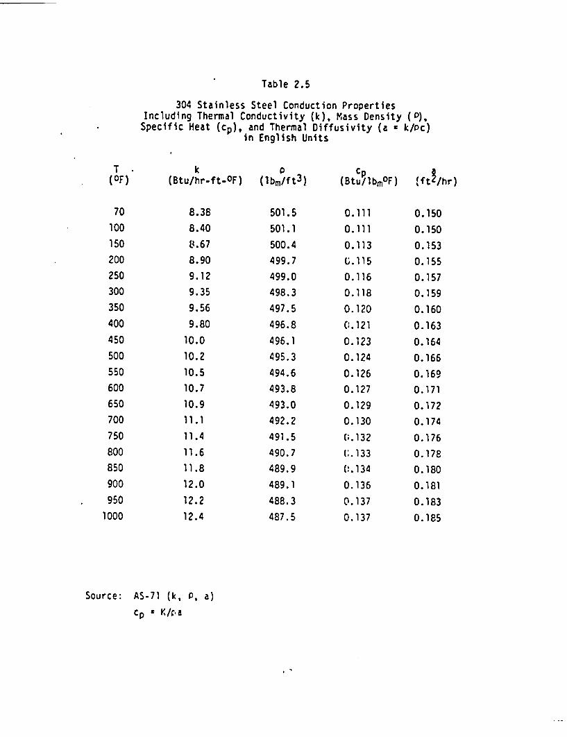
Table 2.5
304 Stainless Steel Conduction PropertiesIncluding Thermal Conductivity (k), Mass Density (),Specific Heat (cp), and Thermal Diffusivity (a k/oc)
in English Units
T -(OF)
70
100
150
200
250
300
350
400
450
500
550
600
650
700
750
800
850
900
950
1000
k(Btu/hr-ft-OF)
8.38
8.40
U.67
8.90
9.12
9.35
9.56
9.80
10.0
10.2
10.5
10.7
10.9
11.1
11.4
11.6
11.8
12.0
12.2
12.4
(lbm/ft 3 )
501.5
501.1
500.4
499.7
499.0
498.3
497.5
496.8
496.1
495.3
494.6
493.8
493.0
492.2
491.5
490.7
489.9
489.1
488.3
487.5
8Btu/lbm°F)
0.111
0.111
0.113
C.115
0.116
0.118
0.120
C:.121
0.123
0.124
0.126
0.127
0.129
0.130
O;.132
(:.133
(0.134
0.136
0.137
0.137
(ftl/hr)
0.150
0.150
0.153
0.155
0.157
0.159
0.160
0.163
0.164
0.166
0.169
0.171
0.172
0.174
0.176
0.178
0.180
0.181
0.183
0.185
Source: AS-71 (k, P, a)
cp K/ra
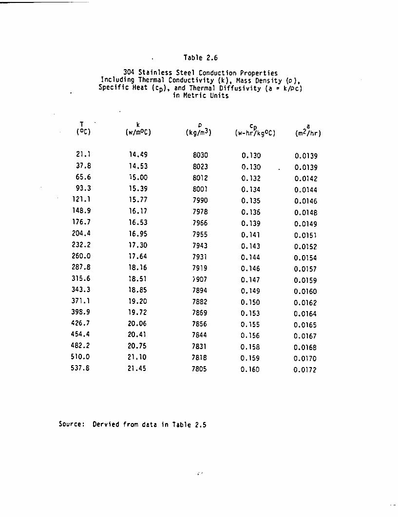
Table 2.6
304 Stainless Steel Conduction PropertiesIncluding Thermal Conductivity (k), Mass Density (o),Specific Heat (cp), and Thermal Diffusivity (a = k/Pc)
in Metric Units
T k P C p a(0C) (W/MOC) (kg/m3) (w-hr/kgOC) (m2/hr)
21.1 14.49 8030 0.130 0.013937.8 14.53 8023 0.130 0.013965.6 15.00 8012 0.132 0.014293.3 15.39 8001 0.134 0.0144
121.1 15.77 7990 0.135 0.0146148.9 16.17 7978 0.136 0.0148176.7 16.53 7966 0.139 0.0149204.4 16.95 7955 0.141 0.0151232.2 17.30 7943 0.143 0.0152260.0 17.64 7931 0.144 0.0154287.8 18.16 7919 0.146 0.0157315.6 '8.51 907 0.147 0.0159343.3 18.85 7894 0.149 0.0160371.1 19.20 7882 0.150 0.0162398.9 19.72 7869 0.153 0.0164426.7 20.06 7856 0.155 0.0165454.4 20.41 7844 0.156 0.0167482.2 20.75 7831 0.158 0.0168510.0 21.10 7818 0.159 0.0170537.8 21.45 7805 0.160 0.0172
Source: Dervied from data in Table 2.5
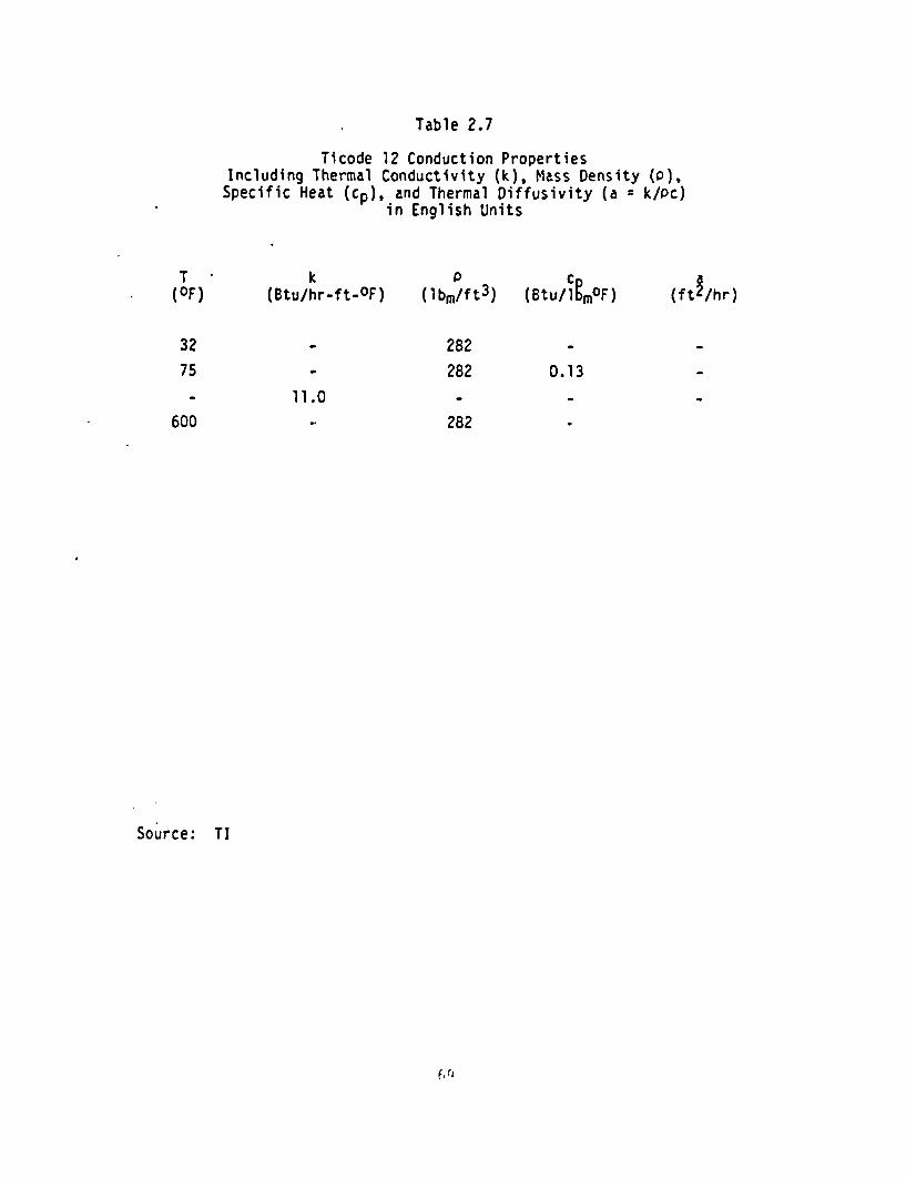
Table 2.7
Ticode 12 Conduction PropertiesIncluding Thermal Conductivity (k), Mass Density (),Specific Heat (cp), and Thermal Diffusivity (a k/Pc)
in English Units
T(OF)
k(Btu/hr-ft-OF) (lb,,/ft3) (Btu/lu F) (ft /hr)
32
75
282
282 0.13
600
11.0
282
Source: TI
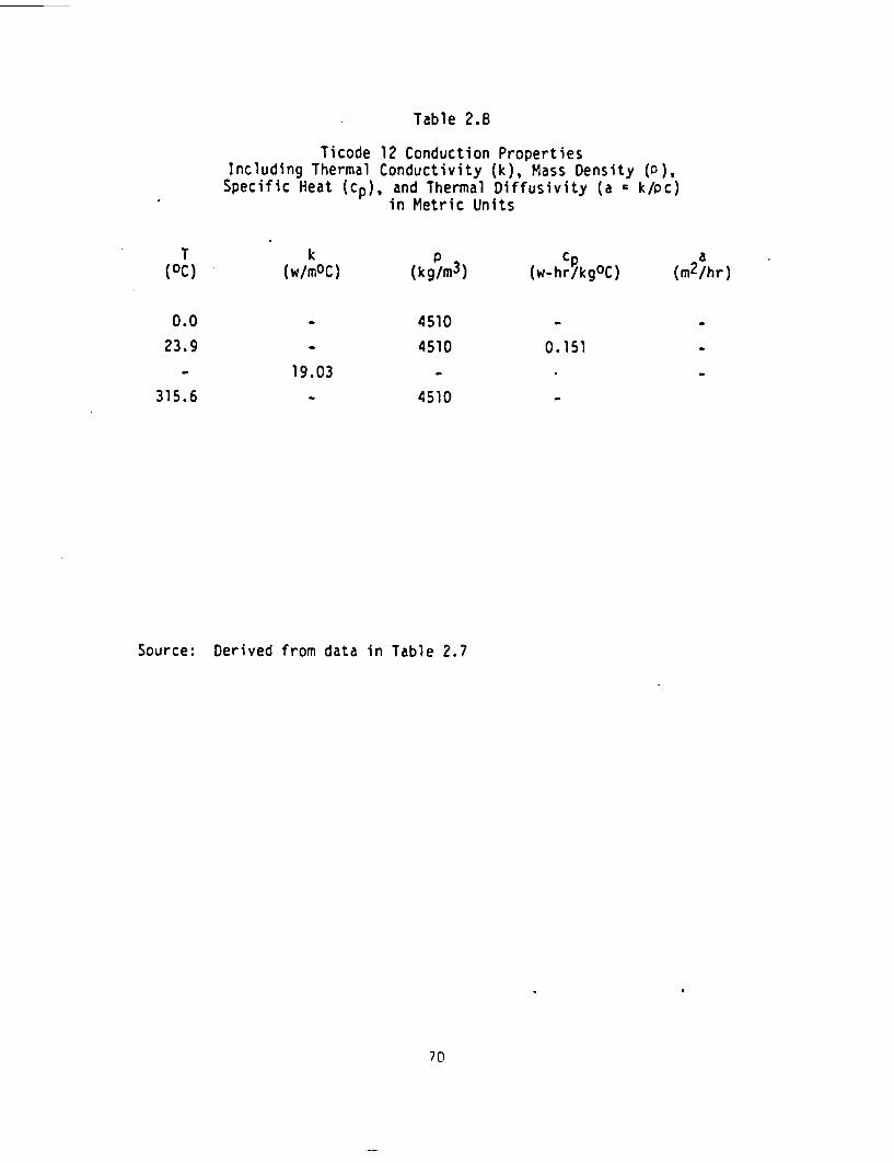
Table 2.8
Ticode 12 Conduction PropertiesIncluding Thermal Conductivity (k), Mass Density (),Specific Heat (cp), and Thermal Diffusivity (a k/oc)
in Metric Units
T(0C)
k(w/mOC) (kg/rm3) Cp(w-hr/kgOC)
a(m2/hr)
0.0
23.9
4510
4510 0.151
315.6
19.03
4510
Source: Derived from data in Table 2.7
70
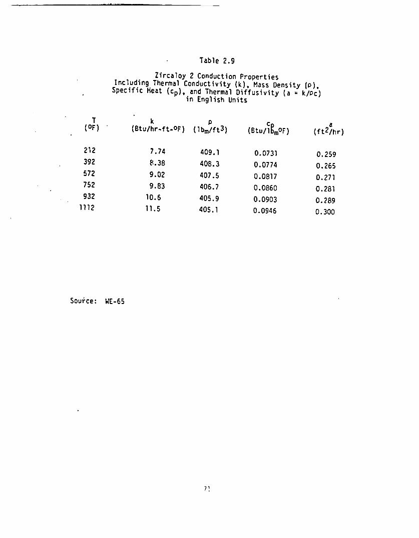
Table 2.9
Zircaloy 2 Conduction PropertiesIncluding Thermal Conductivity (k), Mass Density (),Specific Heat (cp), and Thermal Diffusivity (a = k/Pc)
in English Units
T(OF)
212
392
572
752
932
1112
k(Btu/hr-ft-OF)
7.74
P.. 38
9.02
9.83
10.6
11.5
p(lbm/ft 3 )
409.1
408.3
407.5
406.7
405.9
405.1
CEM(Btu/l1 OF)
0.0731
0.0774
0.0817
0.0860
0.0903
0.0946
a(ft 2 /hr)
0.259
0.265
0.271
0.281
0.289
0.300
Source: WE-65
71

Table 2.10
Zircaloy 2 Conduction PropertiesIncluding Thermal Conductivity (k), Mass Density (p),Specific Heat (cp), and Thermal Diffusivity (a k/pc)
in Metric Units
T(OC)
100
200
300
400
500
600
k(watts/mOC)
13.39
14.49
15.60
: 7.00
18.33
'9.89
(kg/rm3 )
6551
6538
6525
6512
6499
6486
cp(watt-hr/kgOC)
0.0850
0.0900
0.0950
0. 1000
0. 1050
0.1100
(m2/hr)
0.0240
0.0246
0.0252
0.0261
0.0269
0.0279
Source: Derived from data in Table 2.9
72
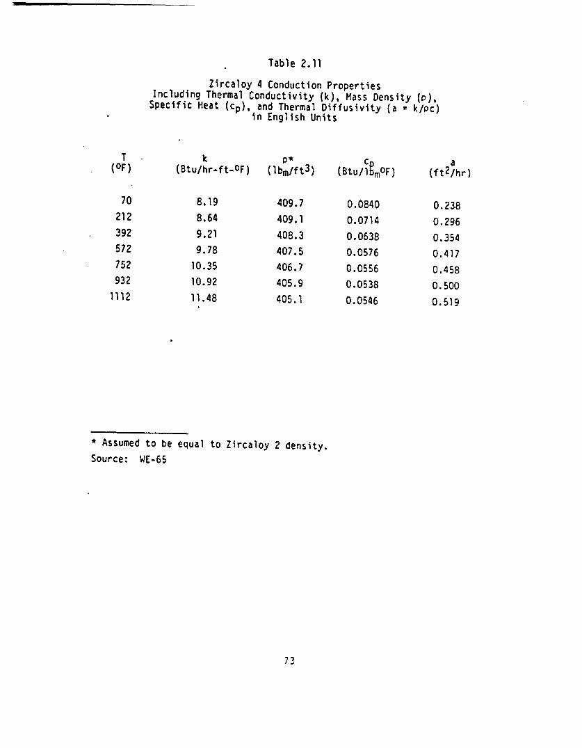
-
Table 2.11
Zircaloy 4 Conduction PropertiesIncluding Thermal Conductivity (k), Mass Density (),Specific Heat (cp), and Thermal Diffusivity (a k/oc)
in English Units
T(OF)
70
212
392
572
752
932
1112
k(Btu/hr-ft-OF)
8.19
8.64
9.21
9.78
10.35
10.92
11.48
P*( lbm/ft 3 )
409.7
409.1
408.3
407.5
406.7
405.9
405.1
(Btu/CIEMOF)
0.0840
0.0714
0.0638
0.0576
0.0556
0.0538
0.0546
a(ft2/hr)
0.238
0.296
0.354
0.417
0.458
0.500
0.519
* Assumed to be equal to Zircaloy 2 density.
Source: WE-65
73
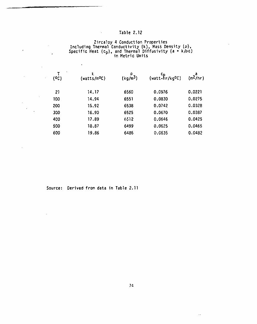
- - - - - -
Table 2.12
Zircaloy 4 Conduction PropertiesIncluding Thermal Conductivity (k), Mass Density (),Specific Heat (cp), and Thermal Diffusivity (a k/ac)
in Metric Units
T(0C)
21
100
200
300
400
500
600
I;(watts/mOC)
14.17
14.94
15.92
16.90
17.89
18.87
19.86
0(kg/m 3)
6560
6551
6538
6525
6 2 12
6499
6486
(watt-hr/kgOC)
0.0976
0.0830
0.0742
0.0670
0.0646
0.0625
0.0635
a(m2 /hr)
0.0221
0.0275
0.0328
0.0387
0.0425
0.0465
0.0482
Source: Derived from data in Table 2.11
74
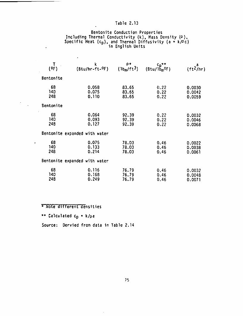
Table 2.13
Bentonite Conduction PropertiesIncluding Thermal Conductivity (k), Mass Density (),Specific Heat (cp), and Thermal Diffusivity (a k/Pc)
in English Units
T(OF)
k(Btu/hr-ft-OF)
( *( bm/f t3) C9**(Btu/l MOF)
a(ft2/hr)
Bentonite
68140248
0.0580.0750.110
83.6583.6583.65
0.220.220.22
0.00300.00420.0059
Bentonite
68140248
0.0640.0930.127
92.3992.3992.39
0.220.220.22
0.00320.00460.0068
Bentonite expanded with water
68140248
0.0750.1330.214
78.0378.0378.03
0.460.460.46
0.00220.00380.0061
Bentonite expanded with water
68140248
0.1160.1680.249
76.7976.7976.79
0.460.460.46
0.00320.00480.0071
* Note different -rensi ties
** Calculated cp k/pa
Source: Dervied from data in Table 2.14
75
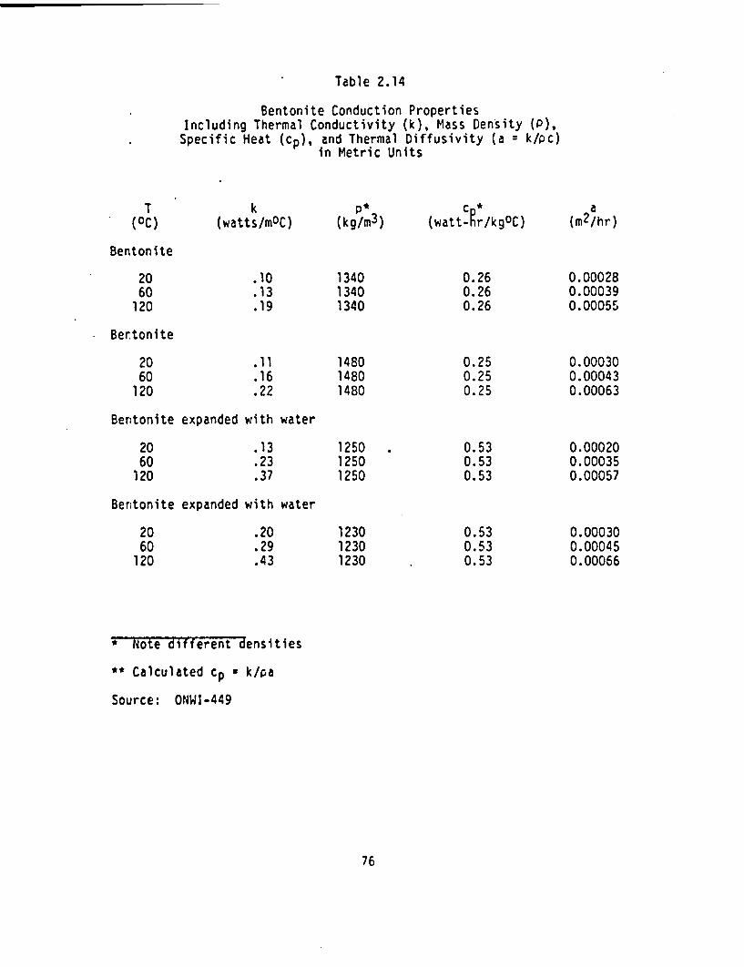
Table 2.14
Bentonite Conduction PropertiesIncluding Thermal Conductivity (k), Mass Density (),Specific Heat (cp), and Thermal Diffusivity (a = k/pc)
in Metric Units
T(0C)
k(watts/mOC)
p*(kg/m3) (watt-hr/kgOC) (m2/hr)
Bentonite
2060120
.10
.13
.19
134013401340
0.260.260.26
0.000280.000390.00055
Bertonite
2060120
.11
.16
.22
148014801480
0.250.250.25
0.000300.000430.00063
Bentonite expanded with water
2060120
.13
.23
.37
125012501250
0.530.530.53
0.000200.000350.00057
Ber;tonite expanded with water
2060120
.20
.29
.43
123012301230
0.530.530.53
0.000300.000450.00066
* Note different densities
** Calculated cp k/pa
Source: ONWI-449
76

Table 2.15
Defense High-Level Waste Glass Conduction PropertiesIncluding Thermal Conductivity (k), Mass Density (),Specific Heat (cp), and Thermal Diffusivity (a k/pc)
in English Units
T(OF)
68
212
392
572
752
932
1112
k(Btu/hr-ft-OC)
0.504
0.562
0.634
0.707
0.779
0.851
0.924
(lbm/ft 3 )
171.7
171.2
170.7
170.2
169.7
169.4
166.8
(Btu/bmOF)
0.196
0.237
0.271
0.296
0.314
0.328
0.338
a(ft 2 /hr)
0.0150
0.0139
0.0137
0.0140
0.0146
0.0153
0.0164
Source: Derived from data in Table 2.16
77

-
Table 2.16
Defense High-Level Waste Glass Conduction PropertiesIncluding Thermal Conductivity (k), Mass Density (),Specific.Heat (cp), and Thermal Diffusivity (a k/oc)
in Metric Units
T(0C)
20
100
200
300
400
500
600
V(watts/moC)
0.872
0.972
1.097
1.222
1.347
1.472
1.598
(kg/m 3 )
2750
2743
2735
2726
2718
2713
2672
(wattchr/kgOC)
0.228
0.276
0.315
0.344
0.365
0.381
0.393
a(m 2/hr)
0.00139
0.00128
0.00127
0.00130
0.00136
0.00142
0.00152
Source: ONWI-423
78
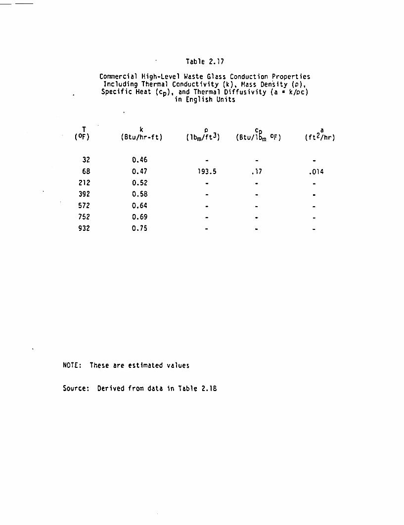
Table 2.17
Commercial High-Level Waste Glass Conduction PropertiesIncluding Thermal Conductivity (k), Mass Density (),Specific Heat (cp), and Thermal Diffusivity (a k/pc)
in English Units
T(OF)
k(Btu/hr-ft) (lbm/ft3) (Btu/igm OF) (ft 2/hr)
32
68
0.46
0.47 193.5 .17 .014
212 0.52
392 0.58
572 0.64
752 0.69
932 0.75
NOTE: These are estimated values
Source: Derived from data in Table 2.18

Table 2.18
Commercial High-Level Waste Glass Conduction PropertiesIncluding Thermal Conductivity (k), Mass Density (),Specific Heat (cp),and Thermal Diffusivity (a k/pc)
in Metric Units
T(0C)
k(watts/mOC) (kg//m 3) (watt-cr/kg OC)
a(m2 /hr)
0
20
100
200
300
400
500
0.8
0.82
0.9
1.0
1.1
1.2
1.3
3100 0.2 0.0013
NOTE: These are estimated values
Source: ONWI-423
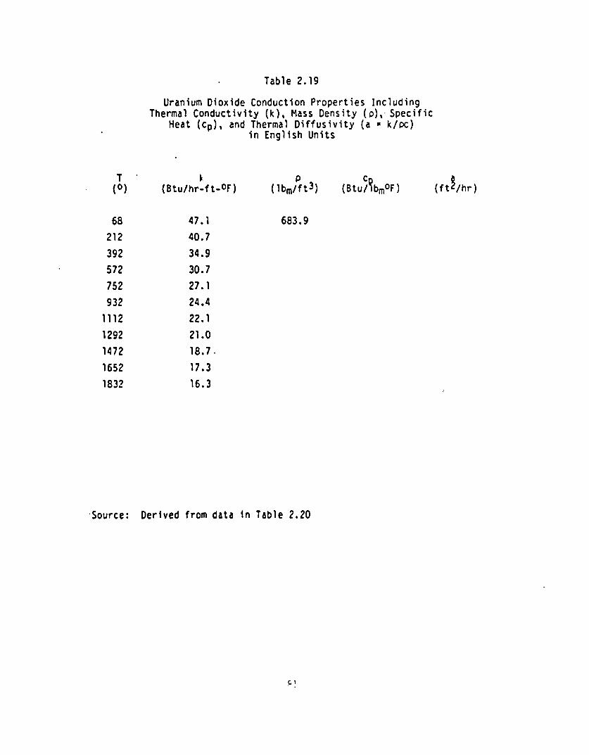
Table 2.19
Uranium Dioxide Conduction Properties IncludingThermal Conductivity (k), Mass Density (p), Specific
Heat (cp), and Thermal Diffusivity (a k/Pc)in English Units
T(0)
68
212
392
572
752
932
1112
1292
1472
1652
1832
(Btu/hr-ft-OF)
47.1
40.7
34.9
30.7
27.1
24.4
22.1
21.0
18.7.
17.3
16.3
P C(lbm/ft 3 ) (Btu/bm0F)
683.9
(ftp/hr)
Source: Derived from data in Table 2.20
c£1
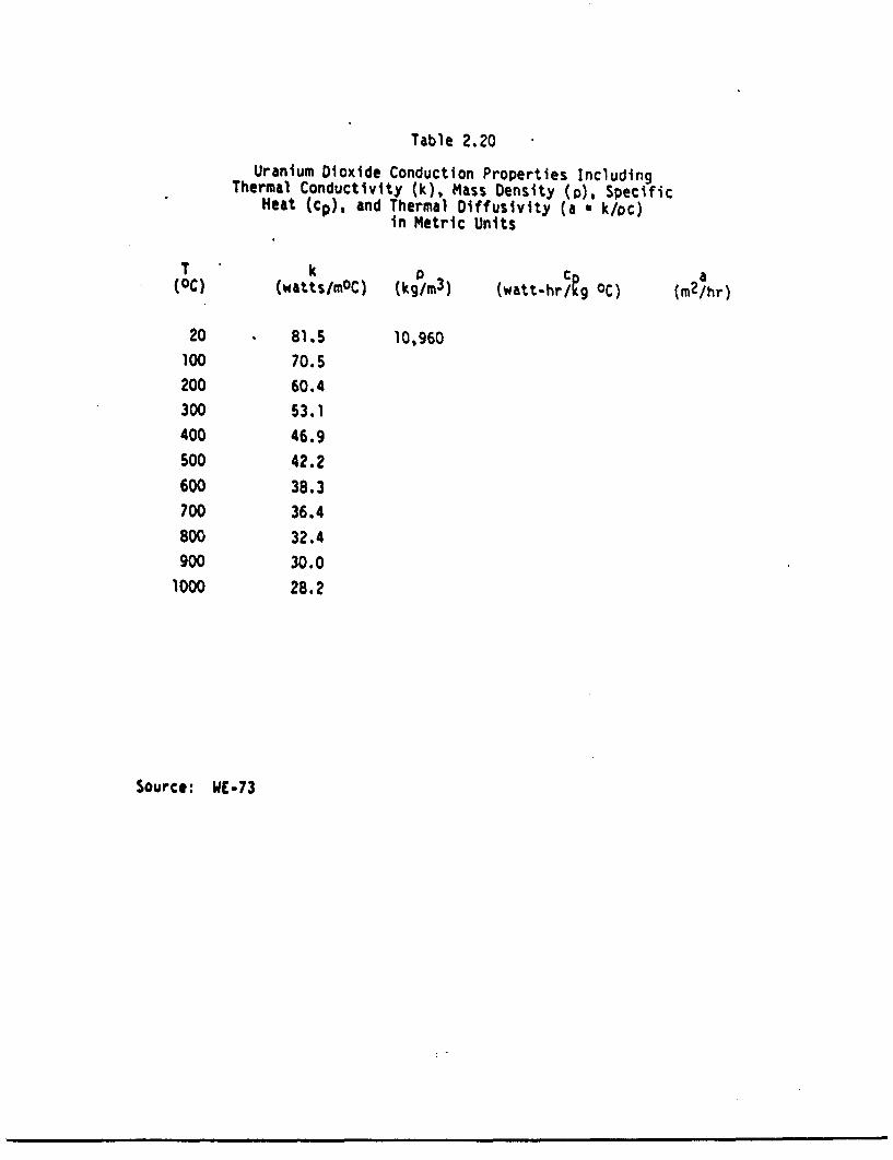
Table 2.20
Uranium Dioxide Conduction Properties IncludingThermal Conductivity (k), Mass Density (p), Specific
Heat (cp), and Thermal Diffusivity (a k/pc)in Metric Units
T(0C)
20100
200
300
400
500
600
700
800
900
1000
k(watts/moC)
81.5
70.5
60.4
53.1
46.9
42.2
38.3
36.4
32.4
30.0
28.2
(kg/rm3 ) (watt-hr/g oC) a(m2/hr)
10,960
Source: WE.73

Table 2.21
Air Thermal Conduction Properties at One Atmosphere PressureIncluding Thermal Conductivity (k), Mass Density (),Specific Heat (cp), and Thermal Diffusivity (a = kC)
in English Units
T(OF)
0
32
100
200
300
400
500
600
700
800
9001000
k(Btu/hr-ft-OF)
0.0133
0.0140
0.0154
0.0174
0.0193
0.0212
0.0231
0.0250
0.0268
0.0286
0.0303
0.0319
(Ibm/ft3) (Btu/lb OF)
0.086
0.081
0.071
0.060
0.052
0.046
0.0412
0.0373
0.0341
0.0314
0.0291
0.0271
0.239
0.240
0.240
0.241
0.243
0.24 5
0.247
0.250
0.253
0.256
0.259
0.262
a(ft 2 /hr)
0.646
0.720
0.905
1.20
1.53
1.88
2.27
2.68
3.10
3.56
4.02
4.50
Source: KR-61
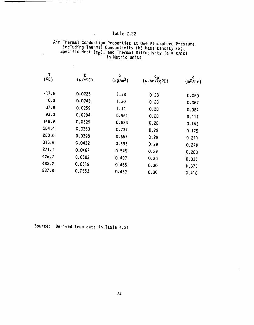
-
Table 2.22
Air Thermal Conduction Properties at One Atmosphere PressureIncluding Thermal Conductivity (k) Mass Density (),
Specific Heat (cp), and Thermal Diffusivity (a k/oc)in Metric Units
T k P (0CT) (W/mOC) (kg/m 3) (w-hr/kgOC) (m2/hr)
-17.8 0.0225 1.38 0.28 0.0600.0 0.0242 1.30 0.28 0.067
37.8 0.0259 1.14 0.28 0.08493.3 0.0294 0.961 0.28 0.111
148.9 0.0329 0.833 0.28 0.142204.4 0.0363 0.737 0.29 0.175260.0 0.0398 0.657 0.29 0.211315.6 (0.0432 0.593 0.29 0.249371.1 0.0467 0.545 0.29 0.288426.7 0.0502 0.497 0.30 0.331482.2 0.0519 0.465 0.30 (1.373537.8 0.0553 0.432 0.30 0.418
Source: Derived from data in Table 4.21
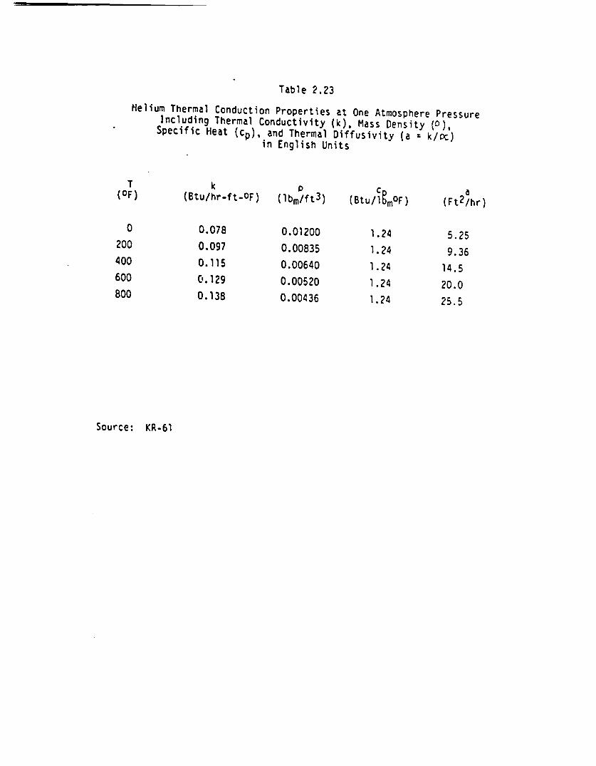
Table 2.23
Helium Thermal Conduction Properties at One Atmosphere PressureIncluding Thermal Conductivity (k), Mass Density (0),Specific Heat (cp), and Thermal Diffusivity (a k/oc)
in English Units
T(OF)
0
200
400
600
800
k(Btu/hr-ft-OF)
0.078
0.097
0.115
'.129
0.138
lIbm/ft3) (Stu/l F)
0.01200
0.00835
0.00640
0.00520
0.00436
1.24
1.24
1 .24
1 .24
1 .24
(Ft 2/hr)
5.25
9.36
14.5
20.0
25.5
Source: KR-61

Table 2.24
Helium Thermal Conduction Properties at One Atmosphere PressureIncluding Thermal Conductivity (k), Mass Density (P),Specific Heat (cp), and Thermal Diffusivity (a s k/Pc)
in Metric Units
T k c0 a(0C) . (w/mOC) (kg//m3) cgoc) (m2/hr)
-17.8 0.135 0.192 1.44 0.488
93.3 0.168 0.134 1.44 0.870
204.4 0.199 0.103 1.44 1.35
315.6 0.223 0.0833 1.44 1.86
426.7 0.239 0.0698 1.44 2.37
Source: Derived from data in Table 2.23

Table 2.25
Saturated Liquid Water Thermal Conduction PropertiesIncluding Thermal Conductivity (k), Mass Density (P),Specific Heat (cp), and Thermal Diffusivity (a k/Pc)
in English Units
T(OF)
32
50100
150
200
250
300
350
400
450
500550
600
k(Btu/hr-ft-OF)
0.319
0.3320.364
0.384
0.394
0.396
0.395
0.391
0.381
0.367
0.349
0.325
0.292
(lbm/ft 3 )
62.4
62.462.0
61.2
60.1
58.8
57.3
55.6
53.6
51.6
49.045.9
42.4
(Btu/bmOF)
1.01
1.000.998
1.001.00
1.01
1.03
1.05
1.08
1.12
1.191.31
1.51
5.07
5.335.88
6.27
6.55
6.69
6.70
6.69
6.57
6.34C.99
5.05
4.57
(ftl/hr)
x 10-3
x 10-3x 10-3
x 10-3
x 10-3
X 10-3
x 10-3
x 10-3
x 10-3
x 10-3
X 10-3x 10-3
x 10-3
Source: KR-61

Table 2.26
Saturated Liquid Water Thermal Conduction PropertiesIncluding Thermal Conductivity (k), Mass Density (),Specific Heat (cp), and Thermal Diffusivity (a = k/pc)
in Metric Units
T(OC)
0.010.037.865.693.3121.1148.9176.7204.4232.2260.0287.8315.6
(w/mOC)
0.5520.5750.6300.6650.6820.6850.6830.6760.6590.6350.6040.5620.505
(kg/im 3)
10001000993980963942918891859827785735679
(w-hr/4g0C)
1.171.161.161.161.161.171.201.221.261.301.381.521.76
a(m2 /hr)
4.72 x4.96 x5.47 x5.85 x6.11 x6.22 x6.20 x6.22 x6.02 x5.91 x5.58 x5.03 x4.23 x
10-410-41o-410-410-410-410-410-410-410-410-410-410-4
Source: Derived from data in Table 2.25
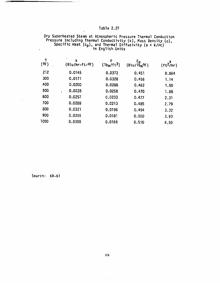
Table 2.27
Dry Superheated Steam at Atmospheric Pressure Thermal ConductionPressure Including Thermal Conductivity (k), Mass Density (),
Specific Heat (cp), and Thermal Diffusivity (a k/Pc)in English Units
T k 0 CD a(OF) (Btu/hr-ft-OF) (Ibm/ft3) (Btu/19MOF) (ft2/hr)
212 0.0145 0.0372 0.451 0.864
300 0.0171 0.0328 0.456 1.14
400 0.0200 0.0288 0.462 1.50
500 . 0.0228 0.0258 0.470 1.88
600 0.0257 C.0233 0.477 2.31
700 0.0288 0.0213 0.485 2.79
800 0.0321 0.0196 0.494 3.32
900 0.0355 0.0181 0.500 3.93
1000 0.0388 0.0169 0.510 4.50
Source: KR-61
P9
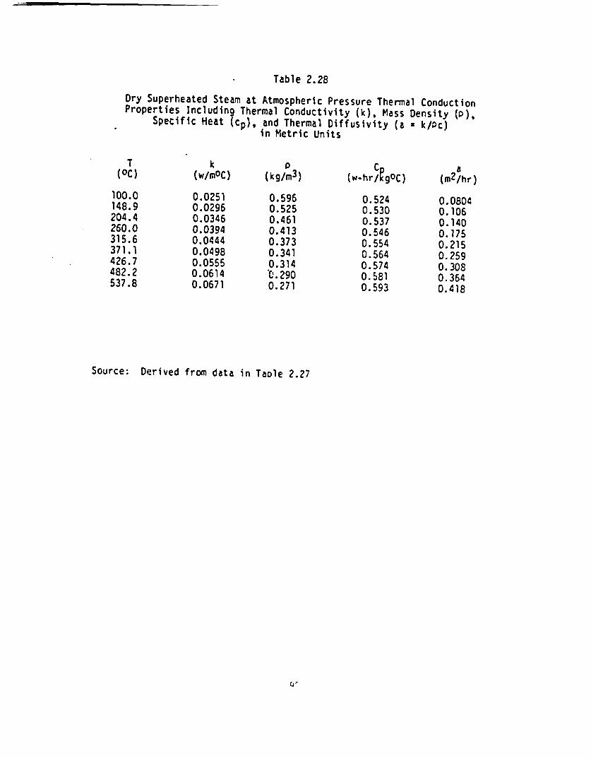
Table 2.28
Dry Superheated Steam at Atmospheric Pressure Thermal ConductionProperties Including Thermal Conductivity (k), Mass Density (),
Specific Heat (cp), and Thermal Diffusivity (a k/Oc)in Metric Units
T k (wh C) am/r(0C) (w/m0C) (kg/rm3) (w-hr/gC ) (m2/hr)
100.0 0.0251 0.596 0.524 0.0804148.9 0.0296 0.525 0.530 0.106204.4 0.0346 0.461 0.537 0.140260.0 0.0394 0.413 0.546 0.175315.6 0.0444 0.373 0.554 0.215371.1 0.0498 0.341 0.564 0.259426.7 0.0555 0.314 0.574 0.308482.2 0.0614 0.290 0.581 0.364537.8 0.0671 0.271 0.593 0.418
Source: Derived from data in Taole 2.27
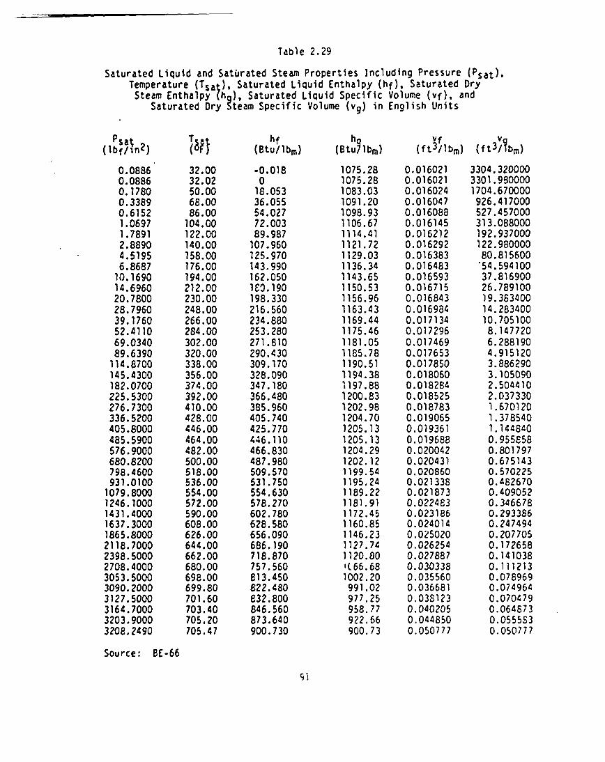
Table 2.29
Saturated Liquid and Saturated Steam Properties ncluding Pressure (Psat).Temperature (Tsat), Saturated Liquid Enthalpy (hf), Saturated DrySteam Enthalpy th ) Saturated Liquid Specific Volume (vf), and
Saturated Dry team Specific Volume (vg) in English Units
(lbf/in2 ) T8?1 hf(Btu/Ibm)
h(BtuN1bm)
Vf(ft 3/lbm) (ft3/bm)
0.08860.08860.17800.33890.61521.06971.78912.88904.51956.868710.169014.696020.780028.796039. 176052.411069.034089.6390114.8700145.4300182.0700225.5300276.7300336.5200405.8000485.5900576.9000680.8200798.4600931.01001079.80001246.10001431.40001637.30001865.80002118.70002398.50002708.40003053.50003090.20003127.50003164.70003203.90003208.2490
32.0032.0250.0068.0086.00104.00122.00140.00158.00176.00194.00212.00230.00248.00266.00284.00302.00320.00338.00356.00374.00392.00410.00428.00446.00464.00482.00500.00518.00536.00554.00572.00590.00608.00626.00644.00662.00680.00698.00699.80701.60703.40705.20705.47
-0.018018.05336.05554.02772.00389.987107.960125.970143.990162.050Io. 90198. 330216.560234.880253.280271.810290.430309.170328.090347.180366.480385.960405. 740425. 770446.110466.830487.980509. 570531.750554.630578.270602. 780628.580656.090686.190718.870757. 560813.450822.480832.800846. 560873.640900. 730
1075.281075.281083.031091.201098.931106.671114.411121.721129.031136.341143.651150.531156.961163.431169.441175.461181.051185.781190.511194.381197.881200.831202.981204.701205.131205.131204.291202.121199.541195.241189.221181.911172.451160.851146.231127.741120.80'(66.681002.20991.02977.25958. 77922.66900.73
0.0160210.0160210.0160240.0160470.0160880.0161450.0162120.0162920.0163830.0164830.0165930.0167150.0168430.0169840.0171340.0172960.0174690.0176530.0178500.0180600.0182840.0185250.0187830.0190650.0193610.0196880.0200420.0204310.0208600.0213380.0218730.0224830.0231860.0240140.0250200.0262540.0278870.0303380.0355600.0366810.0381230.0402050.0448500.050777
3304.3200003301.9900001704.670000926.417000527.457000313.088000192.937000122.98000080.81560054.59410037.81690026.78910019.38340014.28340010.7051008.1477206.2881904.9151203.8862903.1050902.5044102.0373301.6701201.3785401.1448400.9558580.8017970.6751430.5702250.4826700.4090520.3466780.2933860.2474940.2077050.1726580.1410380.1112130.0789690.0749640.0704790.0648730.0555530.050777
Source: BE-66
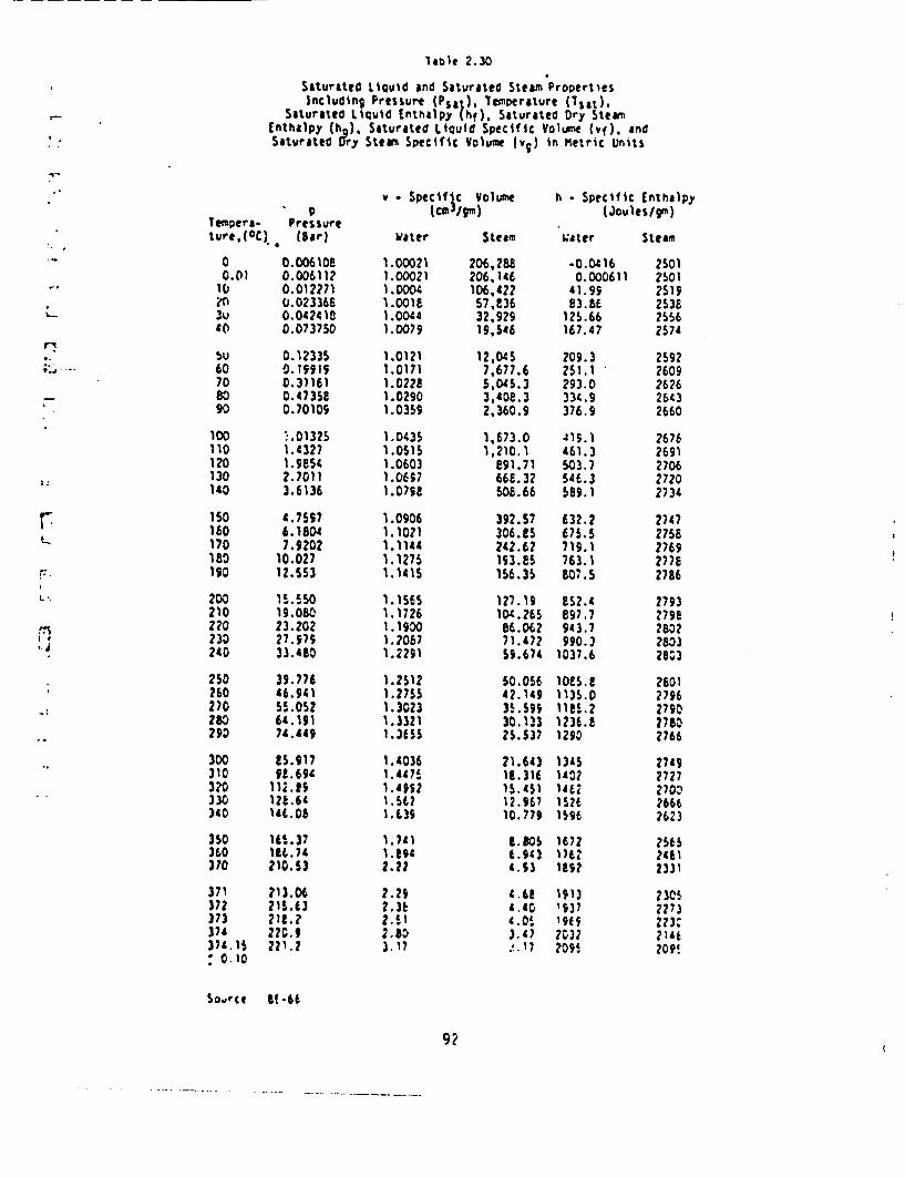
lable 2.30
Saturated Liquid and Saturated Steam PropertiesIncluding Pressure (Psat). Temperature (7)
Saturated Liquid Enthalpy (hf), Saturated Dry SteamInthalpy (hg). Saturated Liquid Specific Volume (), andSaturated DOry Steam Specific Volume (v) in Metric Units
v Specif c Volume h - Specific Enthalpy
Tempera- Pressuretlure(,o) (Bar) Water Steam Water Steam
0 0.006108 1.00021 206,288 -0.0416 25010.01 0.006112 1.00021 206,146 0.000611 25O11( 0.012271 1.D004 106.422 41.99 2519?O U.023366 1.0018 57 36 83.SE 25383v 0.042418 1.0044 32.929 125.66 255640 0.073750 1.0079 19,546 167.47 2574
,' 5u 0.12335 1.0121 12,045 209.3 259260 0.19919 1.0171 7,677.6 251.1 260970 0.31161 1.0221 5,045.3 293.0 2626
_7- sO 0.4735! 1.0290 3,408.3 334.9 264390 0.70109 1.0359 2,360.9 376.9 2660
100 %.01325 1.0435 1,673.0 41S.1 2676110 1.4327 1.0515 1,210.1 461.3 2691120 1.9854 1.0603 E91.71 503.7 2706130 2.7011 1.0697 666.32 546.3 2720140 3.6136 1.0)98 508.66 569.1 2)34
I50 4.7597 1.0906 392.57 632.2 2747160 6.18DA 1.1021 306.85 675.5 2758170 7.9202 1.1144 242.62 719.1 276918o 10.02) 1.1275 193.85 763.1 2778
- 190 12.553 1.1415 156.35 807.5 2786
L. 200 15.550 1.1565 127.19 852.4 2793210 19.080 1.1726 104.265 897.7 2798220 23.202 1.1900 66.062 943.7 2802230 27.979 1.2057 71.472 990.3 2833240 33.480 1.2291 59.674 1037.6 2803
250 39.776 1.2512 50.056 1OES.1 2601260 46.941 1.2755 42.149 1135.0 2)962)0 55.052 1.3023 3S.599 1115.2 2790283 64.191 1.3321 30.133 1236.1 270290 74.419 1.3655 25.537 1290 2766
300 85.917 1.4036 21.643 1345 2749310 91.694 1.44%7 11.316 1402 272732D 112.9 1.4992 15.45) 1462 2703330 2.6' 1.562 12.967 152 2666340 46.08 .I39 10.779 1596 2623
350 115.37 1.741 .8.05 1672 2565360 11.74 .8t4 6.943 176: 2481370 210.53 2.22 4.93 1892 2331
3)1 213.06 2.29 4.6! 113 23C5372 215.63 2.36 4.40 '37 2273373 218.2 2.5' 4.0 19s 223374 220.9 21.0 3.4) 732 2374.15 22'.? 1.17 .17 209S 209!: 0.10
SovtCt St-f6
92

2.2.2 Convection Parameters
Convection data are presented for the following fluids: helium, air,
water, and steam. These data may be used to calculate the convective
heat transfer coefficient, h, so that the rate of heat exchange between
a solid boundary and the fluid in the boundary layer can be evaluated.
The convection heat transfer equation is
q * h A(T - T)
(2.12)
and
* Q/A
(2.107)
where:
¢ a heat flux [e/tL2
q rate of heat transfer from surface to fluid [e/t]
A surface area over which heat transfer is being described [t21
h * heat transfer coefficient e/tt2E6)
T * surface temperature of the solid boundary [e]
T * fluid temperature outside the boundary layer [6]
The convective heat transfer coefficient depends on a variety of param-
eters related to flow conditions, fluid properties, and solid boundary
configurations. In addition, the coefficient will vary with position on
the solid surface. Equations 2.12 and 2.107 prescribe how the heat flux
can be calculated, but it is predicated on the hypothesis that the heat
transfer coefficient can be evaluated. Because the heat transfer coef-
ficient varies with position, it is convenient to evaluate and use the
areal average heat transfer coefficient. Equation 2.22 can be used to
obtain the areal average Nusselt number and Euation 2.21 to obtain the
areal average heat transfer coefficient. Experimentally, heat transfer
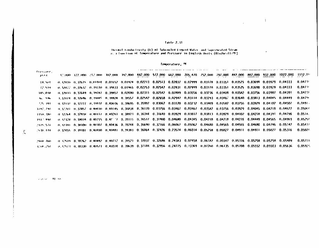
l114a. 7. 1
IIt. u.s1 I su'slss I I IV ( ) I %.sstw #"sII e I qss It W i-e .ssss .sqps I.uts' %I s-A.. . I e I em n I oltesgr jA ' tir e nd Ptt.'.sev in I nq I# %js tI ,t ( It$I si/r ."I)
fewperature* "I
I,%. .1
II. %41
1 4%.n ll
ts,. '19,
'.', 191
h. . -al
t.I .%to
.I 14. hit
I.-.g0tu t'1'.,wu1 .IIII)~ 11A7.00 1397.0100
to. t/t.".
I). 3?/tilt
. 371114
Ii. 171 17
II. t7 3'l I
10. 3745%
11. 1161%
11. 3l 1:
0. 13(49
0. 316%
II. 1717)
t1. 3)IR;
0. 379 1II
n. InIs
n. 8t0lO
0. .138
t).11t 414.
II . 11 llt
0. M9)8
it. t'quI
ti. 49 II) III
ii. 4011 /
0. 4071 %
(i. 40 In0)
0. 4400
0.0 1657
0. 19H.13
0. 39RS7
0. 19970
0. 40 6
0. 40145
0.40761
0.4r 7
0.40436
0.40481
0.01974
0.0 % I 5
0.n?0nnn
0. 33551
0. 38695
0. 311t34
). 3Rs7 I
0. )Ill
0. 19744
0. 39 30 3
4117.000
0.07713
0.02753
0.02313
0.07547
0. 35997
0.116110
0.36344
0.36517
0. 366910
0. 36864
57. 000
0.07513
0.07547
0.02547
0.07658
0.03067
0.03156
0. 31640
0. 319O
0. 37166
0. 3426
667.000)
0 .0831
0.071131
0.07889
0.07947
0.031?0
0.0346)
0.03979
0.046f"0
0.06067
0.?3574
705. 470
0.0?999
0.079q9
0.0.3056
0.03114
0.037 37
0.03461
0.0313 I 1
0.04 345
0.05067
0.06014
157.n01)
0.031)8
0.03l lt
0.03736
0.03793
n.034n9
0.03587
0. 03 3
0.047 18
0.04680
0.052511
79.00n
0.03351
11.03351
0.03409
0.0346-
.0.03587
0.03756
0.03979
0.04?18
0.0456S
0.05072
847.000
0.0.3575
0.03575
0.03587
0.03640
0.03156
0.03979
0.04107
0.04276
0.04565
0.04911
0.0369R
0.03698
0.03756
0.038 13
0.03979
0.04045
0.04218
0.04449
0.04680
0.04911
932.000
0.03979
0 .03929
0.03987
0.04045
0.0410?
0.04718
0.04391
0.04565
0.04196
0.0527
1022.000
0.04 333
0.04333
0.04391
0.04449
0.04507
0. 0467
0.04796
0.04969
0.0514?
0.05316
1112.00
0.047 1)
0.041 V
0.04731
0.04791
0.0491.
0. MY) U
0.0514,
0. (1575f
0.054 1t
0.0560's
0.05171l
0.059?'
*"sN II 11,41 t'l 0.1n37 .40497 (. 401 ' 1.39571 0. 31037 0.376n6 0.74383 0.07458 0.061n? 0.05547 0.05.116 0.05758 0.05?SR 0.05419
tlsI'.,".s iI. t.", ;I 0. 130 t1.4tS%1 .4tLIO 0.3)9639 0.37)84 (.37956 0.24775 0.13369 0.0)760 n.06135 0.05708 0.05552 0.05503 0.05636
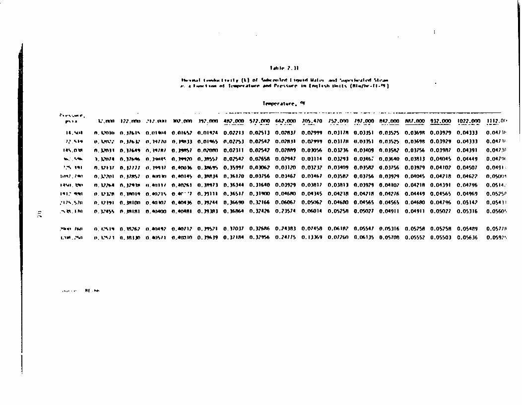
1&hle 7.11
Mel A I 4l.84 II vt li) of wof"Ilrd Ia off ta "4- o '"wo W.lt 4-%I -An
r. Oww Item I n eiwqw atiw ee 1 rtr.. . nql.oh gial (oI/w.Il."l3
Temperature. "t
r... -.r Ia V. 11 1 " .1. Z 1 Zwlan?.Onf nM.41
14. SA" A. lfl1O 0.3761'. 001414 0.024,57 0.01974
14% .0 9
?'4t, gq}
l4%l. Mt
.'11.9.57")
..'% t8. Ilb
0. I.':
0. 3703 I
1. 3r04
0.3VI I
0. V.'.10I
0. 1z4 'a
0. P3 V
0. Q279
0. 3745S
0. MD7
0. 17f41
0. )7t.%
0. 171
0. JRS
0. 3799
0. MI4
0. InIon
0. "11
II. "wI
0. "478
0. 3jqg4
II. IMly
0. AlE) I
o2. 411
0.4071%
0. n VI
0. 400
0. nMl3
0. Ms 7
0. 7
0.400)6
0.40145
0. 4061
0.41- I*
0.4043s
0.404r21
0.01065
0.07080
0. 38'Sl
o.38834
0. 31
0. 3SIIIO."Ill0. 39744
0.." 33
487.00o
0.07238
0.0753
0.02311
0.0427?
0. 35s"
0.36170
0.36344
0. 36517
0. 36640
0. 368h4
517.000
0.0,513
O.OZ54Z
0.02547
O.768sm
0.03067
0.03756
0.31640
0. 31SO
0. I166
0.3476
667.000
0.07831
0.0783
0.07119
0.07947
0.03170
0.03467
0.03979
0.0460
0. 0606
0.73574
s. 4 70
0.07999
0.07m9
0.03056
0.03114
0.03737
0.03467
0.03811
0.0434S
0.05t6?
O.06014
157.0nn
0.03118
0.03112
0.03736
0.03793
0.03409
0.03587
0.03813
0.042 IR
0.04680
0.05758
.... _
0.031I
0.033si
0.03409
0.0346.
0.03517
0.03756
0.03979
0.04718
0.04565
0.05027
847.000
0.03575
0.03575
0.03587
0.03640
0.03156
0.03979
0.04107
0.04776
0.04565
0.0491 1
M7.000
0.0369R
0.03698
0.03156
0.03813
0.03979
0.04045
0.04218
0.04449
0.04680
0.04911
932.000
0.03979
0.03929
0.03987
0.0404S
0.04107
0.04Z18
0.04391
0.04565
0.04796
0.05027
102.000
0.04333
0.04333
0.04391
0.04449
0.04507
0.046z7
0.04?96
0.04969
0.05147
0.05316
1112.0"
0.0471i
0.04 1V
0.0473P
0.0479
0.04911
n. OW)
0.05 14.'
0.0525P
0.05431
0.0560l.
0.0577F
0.05975S
.?,U9 16n 0.7%I% 0.9o 67 o 04497 0.40?17 0.39571 0.317037 0.37 6 0.74383 0.07458 0.0618 0.05547 0.05316 0.05pSM 0.05258 0.054n9
.lI ..40 &).3%il 0.3A330 0.4syI 0.4tnm0 0.39"39 0.37184 0.379S6 0.24775 0.13369 0.017(0 0.06135 0.05708 0.05552 0.05503 0.05636
I
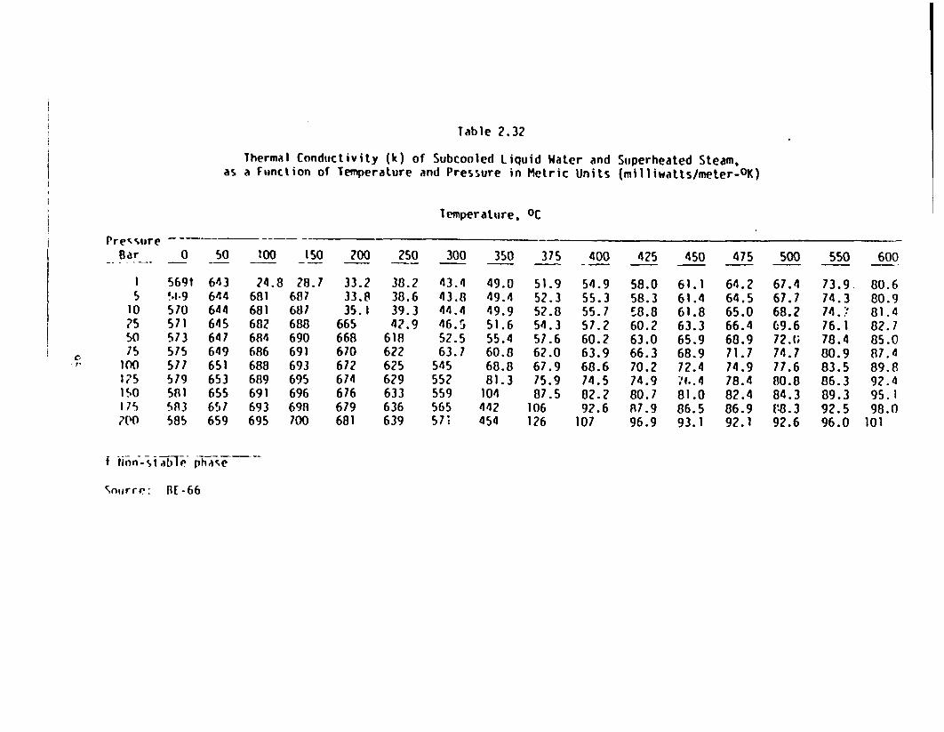
Table 2.32
Thermal Conductivity (k) of Subcooled Liquid Water and Superheated Steam.as a Function of Temperature and Pressure in Metric Units milliwatts/meter-OK)
Temperature, OC
re --i're6Bar 0 50 100 IS0 200 250 300 350 375 400 425 450 475 500 550 600
I 569t 643 24.8 28.7 33.2 38.2 43.4 49.0 51.9 54.9 58.0 61.1 64.2 67.4 73.9. 80.65 !.1.9 644 681 687 33.8 38.6 43.8 49.4 52.3 55.3 58.3 61.4 64.5 67.7 74.3 80.910 570 644 681 687 35.1 39.3 44.4 49.9 52.8 55.7 58.8 61.8 65.0 68.2 74.! 81.475 571 645 682 688 665 42.9 46.5 51.6 54.3 57.2 60.2 63.3 66.4 69.6 76.1 82.7so 573 647 684 690 668 618 52.5 55.4 51.6 60.2 63.0 65.9 68.9 72.(; 78.4 85.075 575 649 686 691 670 622 63.7 60.8 62.0 63.9 66.3 68.9 71.7 74.7 80.9 87.4
100 577 651 688 693 672 625 545 68.8 67.9 68.6 70.2 72.4 74.9 77.6 83.5 89.8175 579 653 689 695 674 629 552 81.3 75.9 74.5 74.9 f.. 4 78.4 80.8 86.3 92.410 581 655 691 696 676 633 559 104 87.5 82.2 80.7 81.0 82.4 84.3 89.3 95.1175 S83 657 693 698 679 636 565 442 106 92.6 R7.9 86.5 86.9 V8.3 92.5 98.0700 585 659 695 700 681 639 571 454 126 107 96.9 93.1 92.1 92.6 96.0 101
Snjrre: BE-66

Table 2.33
Specific Volume (v) of Sbcooled Liquid Water and SuperheatedSteam as a Function of Temperature and Pressure
in English Units ft3/lbm)*
Temperature, OF
Pressurepsid 32.000 122.000 212.000 302.000 392.000 482.000 572.000 662.000
'.C
14.50412.519
145.038362.596125.1911087.7901450.3801812.9807175.5702538. 170
0.016020.016020.016010.016000.015980.015%60.015940.015920.015900.01588
0.016210.016210.016200.016190.016180.016160.016140.016120.016110.01609
27. 1660.016710.016710.016700.016670.016650.016640.016620.016600.01657
31.0110.017470.017460.017450.017420.017400.017370.017350.011320.01730
34.8076.8093.3000.018510.018470.018430.0 18390.0 18360.0 18320.01828
38.539307.5983.7271.3940.020010.019950.019880.019810.019740.01968
42.271508.369414.131041.5840.7260.4280.022380.022220.022070.02193
45.987709.131864.523481. 757170.8320.5200.3590.2580.1840.02749
2900.760 0.01586 0.01607 0.01656 0.01727 0.01823 0.01962 0.02178 0.026673?(18.250 0.01585 0.01606 0.01654 0.01725 0.01821 0.01958 0.02168 0.02619
' t-tl iIeWJ --n, -ne-xt rpaige -
rotircr: IE-66

Table 2.33 (continued)
Temperature, F
Pressure_ psia
14.50472.519
145.038362.596725.191
1087.7901450.3801812.9802175.5102538.170
705.470 752.000 797.000 842.000 887.000 932.000 1022.000 1112.000
47.782609.491034.710711.837640.817770.555370.391780.291180.2210.168
49.703909.886314.9063311.922160.925200.591220.422870.320520.250680.19958
51.5459010.261105.100132.002250.969570.624060.450430.345350. 274550.22313
53.4040010.63760
5.290752.082341.012980.655620.476210.368090.295530.24331
55.2621011. 009205.481362.162431.055430.686050.500720.389400. 314 750.26125
57.1042011. 385605.670372.240921.097230.715840.524750.416310.333170.27807
60.8203012.132006.043592.396291.179080.773350.570400.448340.366970.30883
64.5205012.876906.423322.550071.259340.829090.613810.484700.398530.33702
2900.760 0.120 0.15938 0.18373 0.20359 0.22089 0.23675 0.26510 0.29089.3208.250 0. 5018 0.13099 0.15710 0.17710 0.19399 0.20931 0.23617 0.26046

Table 2.34
Speilic Volume () of Subcooled Liquid Water and Superheated Steam as Functionof Temperature and Pressure In Metric Units ( 3 /g)
temperature. OC
oaf 0 50 100 150 200 250 300 350 315 400 425 450 475 500 550 6(X)
I 1.0007 1.01?1 1696 1936 213 2406 At39 281 79e 3103 3218 3134 3450 3565 319 4078
5 0.9999 1.0119 1.0433 1.0906 475.1 414.4 522.5 510.1 593.1 61t.2 640.6 664.1 681.5 10.8 15.4 803.9
to 0.9991 1.011) 1.0431 1.0903 2U6.0 232.1 251.9 282.4 294.S 306.S 318.4 330.3 342.2 354.0 It.5 401.0
ZS 0.9989 1.0110 1.0473 1.0094 1.15S6 87.0 98.9 109.t 114.9 120.0 125.0 130.0 13S.0 139.9 149.6 159.?
50 0.9916 100)99 1.0410 I t8 1.151 1.2495 45.34 51.93 54.90 51.t6 60.53 63.24 65.89 68.50 13.61 18.62
JS 0.9964 1.0051 1.0398 1.862 1.150) 1.2452 26.)1 3Z.44 34.15 36.91 318.96 40.93 42.83 44.69 48.28 51.16
100 0.9952 10011 1.0386 1 0046 1.1483 1.2409 1.397 22.44 24.53 26.40 28.12. 29.13 31.26 32.t6 3S.61 35.3?
iS 0.9940 1.004.6 1.0313 I O10 1.1460 1.2361 1.3R1 16.14 18.25 20.01 21.56 22.90 24.31 2S.59 2t.99 30.2t
ISO 0.9978 I oSS 1.0361 1.0813 1.1416 1.2371 1.3t8 11.49 13.91 15.65 11.14 18.45 19.65 20.80 22.91 24.18
uis 0.9915 I.Ou44 1.0348 1 098 1.1414 1.2288 1.369 1.t16 !0.5t 12.46 13.93 15.19 16.11 11.36 19.28 21.04
.A ) 0.9904 1.03 1.0 16 I.0/87 1.1391 1.2251 1.360 1.665 .68 9.95 11.41 12.11 13.19 14.78 16.S5 15.16
. ( fl 66

Table 2.35
Specific Enthalpy (h) of Subcooled Liquid Water andSuperheated Steam as a Function of Temperature and Pressure
in English Units (Btu/libm)*
Temperature, OF
32.000 122.000 212.000 302.000 392.000 482.000 572.000 662.000Pressure,
psia
14.50472.519
145.038362.596725.1911087.7901450.3801812.98;2175.5702538.170
0.0260.20?0.4211.0752.1713.2594.3425.4176.4927.567
89.98790.116'0.33190.84791.79392.7 -
93.68594.58795.49096.436
1150.53180.318180.447181.006181.780182.597183.414184.231185.047185.864
1193.95271.810271.896272.326272.971273.659274. 347275.035275. 722276.410
1236.521228.351216.74366.655367.085367.601368.074368.547369.020369.536
1279.0801273.061265.321238.67466.832466.875466.918466.961467.047467.133
1321.6401317.3501311.7601293.701257.581209.86577.413576.124575.264574.404
1365.0701362.0601357. 7601344.0001319.071291.121257.151215.021157.41714.995
'0%0
2900.760 8.64? 97.382 186.681 277.098 370.009 467.262 573.544 707.6863208.250 9.553 98.148 187.374 277.682 370.446 467.444 572.815 702.946
Continued on next page
Source: BE-66
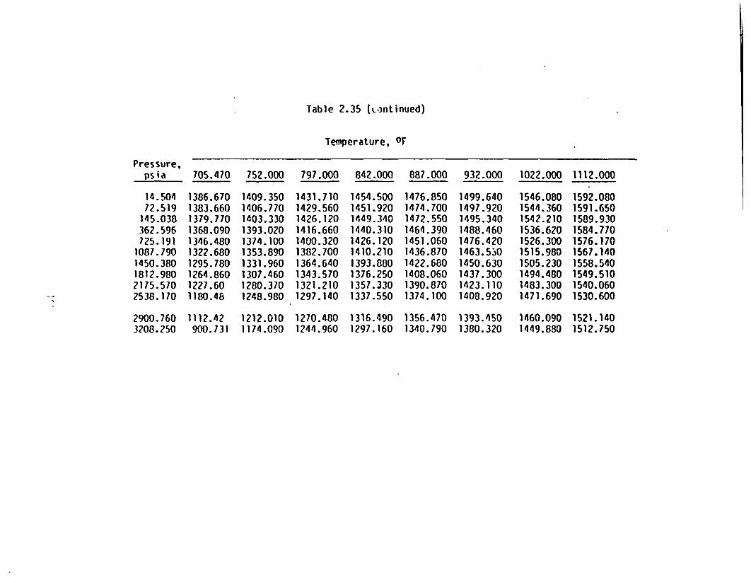
Table 2.35 (ntinued)
Temperature, OF
Pressure,psia 705.470 752.000 797.000 842.000 887.000 932.000 1022.000 1112.000
14.50472.519145.038362.596725.1911087. 7901450.3801812.9802175.5702538.170
1386.6701383.6601379.7701368.0901346.4801322.6801295.7801264.8601227.601180.48
1409.3501406.7701403.3301393.0201374.1001353.8901331.9601307.4601280.3701248.980
1431.7101429.5601426.1201416.6601400.3201382.7001364.6401343.5701321.2101297.140
1454.5001451.9201449.3401440.3101426.1201410.2101393.8801376.2501357.3301337.550
1476.8501474.7001472.5501464.3901451.0601436.8701422.6801408.0601390.8701374.100
1499.6401497.9201495.3401488.4601476.4201463.5301450.6301437.3001423.1101408.920
1546.0801544.3601542.2101536.6201526.3001515.9801505.2301494.4801483.3001471.690
1592.0801591.6501589.9301584.7701576.1701567.1401558.5401549.5101540.0601530.600
2900.760 1112.42 1212.010 1270.480 1316.490 1356.470 1393.450 1460.090 1521.1403208.250 900.731 1174.090 1244.960 1297.160 1340.790 1380.320 1449.880 1512.750
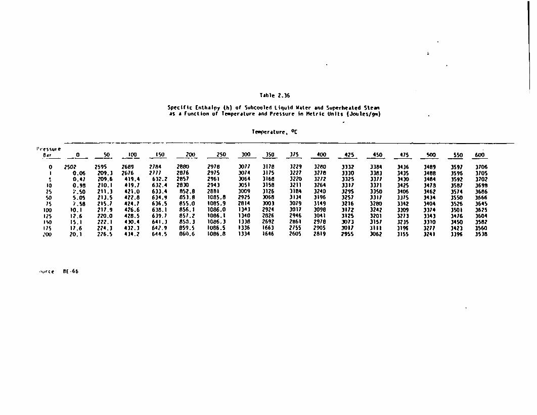
TSble 2. 6
Specific Enthalpy (h) f Subcoulcd iquid Wter and Superhweated Steamas a Function of Temperature and Pressure in Metric Units (Joules/go)
Temperature. C
I'r essu C8r O SO 100 15O 200 250 300 350 375 400 425 450 475 4n0 550 600
0 2502 2595 2689 2784 2880 2978 3077 3178 3229 3280 3332 3384 3436 3489 3597 31061 0.06 209.3 2676 271 2876 2975 3074 3175 3227 3218 3310 3383 3435 3488 3596 3705
0.47 209.6 419.4 632.2 2857 2961 3064 3168 3220 32172 3325 31Z 3430 3484 3592 370210 0.98 210.1 419.7 632.4 2830 2943 3051 3158 3211 3264 3317 3371 3425 3418 3587 369825 ;.50 211.3 421.0 633.4 852.8 2881 3009 3126 3184 3240 3295 3350 3406 3462 3574 3686SO 5.05 213.5 422.8 634.9 53.8 1085.8 2925 3068 3134 3196 3257 3311 3175 3434 3SSO 366675 i.58 21S.7 424.1 636.5 855.0 1085.9 2814 3001 3079 3149 3216 3280 3342 3404 3526 364S
100 10.1 217.9 426.6 638.1 856.1 1086.0 1343 2924 3017 3098 3172 3242 3309 3374 3501 3625125 12.6 220.0 428.5 639.7 857.2 1086.1 1140 2026 2946 3041 3125 3201 3213 3343 3416 3604ISO 15.1 222.1 4)0.4 641.3 853.3 1086.1 1338 2692 2861 2918 3013 3151 3235 3310 3450 3582175 17.6 224.3 432.3 642.9 859.5 1086.5 1336 1663 2755 2905 3011 3111 3196 3277 3421 3560:W 20.1 226.5 434.2 644.5 860.6 1086.8 1334 1646 2605 2819 2955 3062 3155 3241 396 358
Oor Ce: BE 66
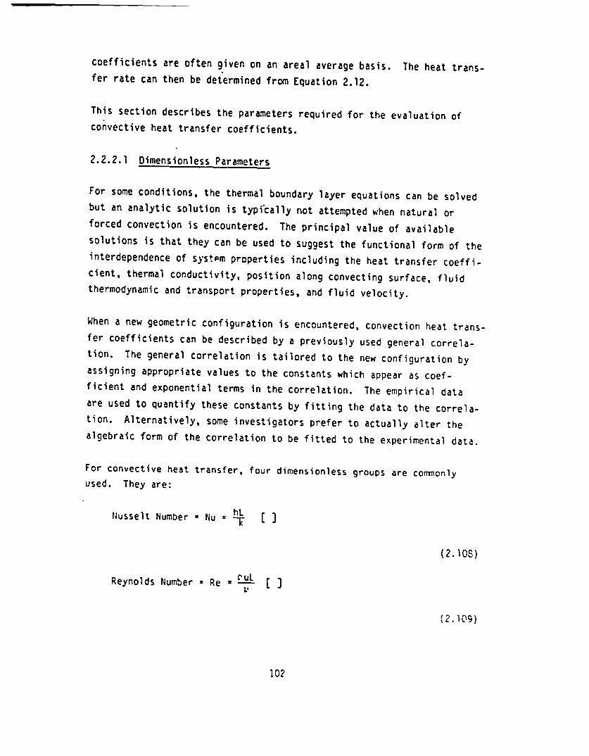
coefficients are often given on an areal average basis. The heat trans-
fer rate can then be determined from Equation 2.12.
This section describes the parameters required for the evaluation of
convective heat transfer coefficients.
2.2.2.1 Dimensionless Parameters
For some conditions, the thermal boundary layer equations can be solved
but an analytic solution is typically not attempted when natural or
forced convection is encountered. The principal value of available
solutions is that they can be used to suggest the functional form of the
interdependence of system properties including the heat transfer coeffi-
cient, thermal conductivity, position along convecting surface, fluid
thermodynamic and transport properties, and fluid velocity.
When a new geometric configuration is encountered, convection heat trans-
fer coefficients can be described by a previously used general correla-
tion. The general correlation is tailored to the new configuration by
assigning appropriate values to the constants which appear as coef-
ficient and exponential terms in the correlation. The empirical data
are used to quantify these constants by fitting the data to the correla-
tion. Alternatively, some investigators prefer to actually alter the
algebraic form of the correlation to be fitted to the experimental data.
For convective heat transfer, four dimensionless groups are commonly
used. They are:
Nusselt Number = Nu = ]
(2.10S)
Reynolds Number Re - , j
(2.109)
102
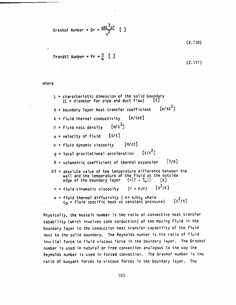
oS3AGrashof Number Gr 2 - -
V
(2.110)
Prandtl Number Pr * a )(2.111)
where
L = characteristic dimension of the solid boundary(L diameter for pipe and duct flow) [t]
h boundary layer heat transfer coefficient [e/tt2J
k = fluid thermal conductivity [e/tte]
0 = fluid mass density [m/23]
u * velocity of fluid [L/t]
Ii fluid dynamic viscosity [m/t]
g - local gravitational acceleration [f/t2)
B - volumetric coefficient of thermal expansion [l/e]
AT- =absolute value of the temperature difference between thewall and the temperature of the fluid at the outsideedge of the boundary layer (=IT - T,) [el
v a fluid kinematic viscosity (V = /o) [t2/t]
a = fluid thermal diffusivity ( a k/opc where 2cp fluid specific heat at constant pressure) [t It)
Physically, the Nusselt number is the ratio of convective heat transfer
capability (which involves some conduction) of the moving fluid in the
boundary layer to the conduction heat transfer capability of the fluid
next to the solid boundary. The Reynolds number is the ratio of fluid
in(ritial force to fluid viscous force in the boundary layer. The Grashof
number is used in natural or free convection analogous to the way the
Reynolds number is used in forced convection. The Grashof number is the
ratio of buoyant forces to viscous forces in the boundary layer. The
103
Prandtl number is a property of the fluid. It is the ratio of the kine-
matic viscosity to the thermal diffusivity.
The volumetric coefficient of thermal expansion is defined as
F 1p)
P
v T)
I for an ideal gas(2.112)
where
B = volumetric coefficient of thermal expansion [I/9
v specific volume [3 /m]
For fluids which do not behave as ideal gases, can be approximated as
P0z -0PE p(T - T.)
co VT-TX (2.113)
in terms of conditions on both edges of the boundary layer, where
T, v, and are the fluid temperature, specific volume and mass density.
These properties are valuated at the film temperature defined as the
average between the wall temperature Tw and the free stream temperature
To.
Many other dimensionless groups are used in describing convection, but
they are less common than the four just presented. These groups include:
104

Stanton Number = St 3 h
(2.114)u L
Peclet fnumber = Pe = Re Pr = Oi
(2.115)
Rayleigh umber Ra GrPr 96L 6TV
(2.116)
4Modified Grashof umber = Gr = GrNu = qL Th
Vk(2.117)
2.2.2.2 Forced Convection
Section 2.1.2.1 presented the laminar boundary layer equations for a
flat plate with a solution given by Blasius. The work of Nusselt (about
1915) led to the completely non-dimensional form of the forced convection
equation, which was stated as
Nu = C Rem Prn
(2.118)
where C, m, and n are constants.
This general form is rather common for the turbulent as well as the
laminar boundary layers for both external surfaces (i.e., unconfined
flow) such as walls and for internal surfaces (i.e., confined flow) such
as pipes or ducts. For confined flow in ducts or pipes, the diameter is
typically used as the characteristic dimension in the Nusselt and Reynolds
numbers in place of characteristic length, L, or position, x, measured
in the downstream direction.
If the duct is not round, the hydraulic diameter, Dh, is used where
D g 4 (flow area)h wetted perimeter)
(2.119)
1nr

Typically, the objective of laboratory experiments is to define the
parameters C, m, and n for a given convection configuration and flow
conditions.
In a pipe, the transition from laminar flow to turbulent flow occurs
when the Reynolds number (based on the areal average flow velocity)
reaches a value of about 2,000 to 3,000. A value of 2,300 is commonly
used in engineering analyses. For a flat plate, when the Reynolds number
is based on a characteristic length equal to the plate dimension in the
flow direction, the laminar to turbulent flow transition usually occurs
in the range 100,000< ReL < 1,000,000. In engineering analyses, a value
of 3.2 x 10⁵ is commonly assumed to be representative.
In the upstream region of the plate, the boundary layer is laminar. The
heat transfer is excellent at the leading edge but diminishes rapidly in
the downstream direction as shown in Figure 2.7 until the transition to
turbulent flow occurs. The heat transfer diminishes because the lamina
that are established in this region support a temperature gradient and
tend to insulate the plate. In the transition region, the flow lines
are broken up by fluid swirl and less temperature gradient can be sus-
tained across the boundary layer. Downstream where turbulence is es-
tablished, the fluid is well mixed and contacts the surface at a high
frequency and thus acts as a colder and/or more accessible sink than in
the laminar region. This discussion assumes the plate to be hot and the
fluid cold.
The heat transfer rate increases very rapidly in the transition region.
Figure 2.7 shows these regions and qualitatively indicates how the heat
transfer rate varies with axial position. This figure illustrates the
relatively high average heat transfer rate that can be sustained in the
turbulent boundary layer region. The laminar region is not very effective
for heat transfer because the transfer rate diminishes rapidly with
distance along the plate in the flow direction and tends to have a small
average value. For these reasons, most heat transfer equipment is de-
signed for turbulent flow and higher heat transfer coefficients with the
associated higher convection heat transfer rates.
106
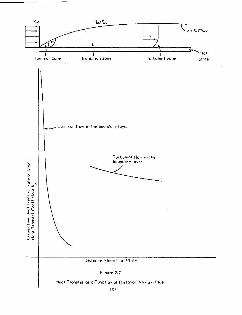
Us0 U o70600
0.?OU00
fflot
pInte
Larninor flow in the boundary layer
Turbulent flow in heboundary lyer
A.-
-
c A.
E
cc .=c_
.N_
.W.
c ,>
cE E
I
-4.
Distonre Alonn F oi "lnIe
Fioure 2.7
Heat Transfer as a Function of Distance
107
A lonq o Ploti

As the thermal boundary layer increases to equal the inside radius in
pipe flow, the free stream no longer exists. Thus, T is not used in
pipe flow as the fluid reference temperature for convection calculations.
The fluid reference temperature is based on the average temperature of
all the mass flowing past a given cross-section of the pipe and is re-
ferred to as the bulk fluid temperature Tb given by
R
b R
f PU(r)c prdr
(2.120)
where
p = fluid mass density fm/i ]
u(r) = fluid velocity which is a function of radiusat any cross-section [/t)
cp constant pressure specific heat of the fluid [e/m*3
T fluid temperature [e)
R inside radius of pipe [z)
r = denotes radial position in the flow stream [I]
A similar relationship would be used for flow channels that are not
round. The heat transfer rate between the tube wall and the fluid
flowing in the pipe is given by
q hA (Tw - Tb).
(2.12)
Ir regions where the boundary layer thickness is much smaller than the
distance separating solid surfaces, non-planar surfaces are often treated
as flat plates.
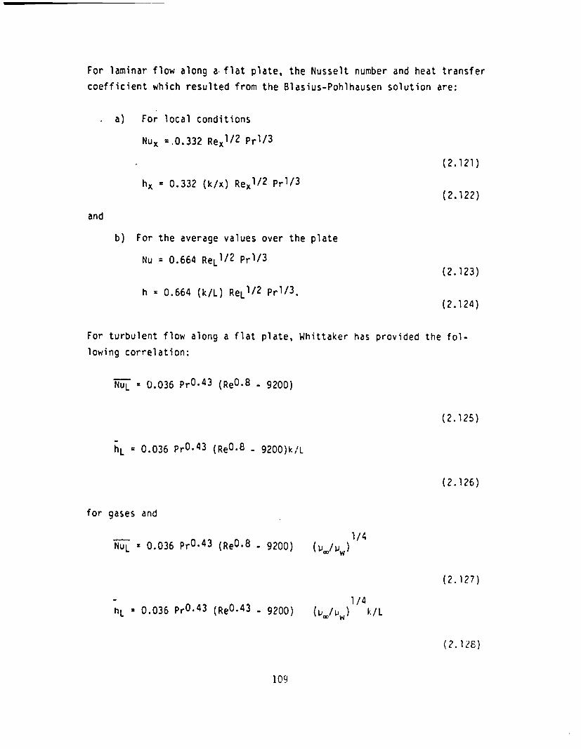
For laminar flow along a flat plate, the Nusselt number and heat transfer
coefficient which resulted from the Blasius-Pohlhausen solution are:
a) For local conditions
Nux = 0.332 Rexl/2 Prl/ 3
(2.121)
hx = 0.332 (k/x) Rexl/2 PrI/ 3
(2.122)
and
b) For the average values over the plate
Nu = 0.664 ReL /2 Prl/3
(2.123)
h = 0.664 (k/L) ReL1/2 Prl/3.(2.124)
For turbulent flow along a flat plate, Whittaker has provided the fol-
lowing correlation:
NuL 0.036 PrO-43 (ReO. - 9200)
(2.125)
hL 0.036 PrO-43 (Re0-8 - 9200)k/L
(2.126)
for gases and
NuL 0.036 PrO-43 (Re0*8 - 9200)
hL 0.036 PrO-43 (ReO-43 - 9200)
1/4
(Ij.A/ w )
(2.127)
1/4(W.u/I'w) k/L
(2.128)
109

for liquids. Except for the viscosity correction term, all fluid prop-
erties are evaluated at the film temperature f defined as
Tf = (Tw + T/2
(2.129)
where
Tw wall temperature [el
TX = free stream temperature (el
For laminar flow
can be solved to
in a pipe, at low Reynolds numbers, the energy equation
give an exact solution for the Nusselt Number.
Nud kd/k
(2.130)
Nud 4.36
(2.131)
h a 4.36k/d
(2.132)
In 1930, Dttus and Boelter correlated the heat transfer coefficient for
convection with turbulent flow inside automobile radiator tubes. The
correlation is widely accepted and used for flow in ducts, channels,
pipes, etc., and is given by
RnUd 0.023 edO.8 PrO.4
(2.133)
1 1 r
hd 0.023 Red0 .8 PrO.4 (k/d)
(2.134)
where the fluid properties are based on the fluid bulk temperature given
by Equation 2.120.
Numerous correlations are available for various boundary configurations,
flow conditions and parameter ranges.
This report presents representative correlations. The waste package
thermal analysts will need to consult other sources for comprehensive
treatment of forced convection correlations.
2.2.2.3 Natural Convection
Natural convection was described in Section 2.1.2.2. A principal dif-
ference between natural and forced convection is that the velocity profile
diminishes to zero at the outer edge of the thermal boundary layer in
natural convection. In forced convection, it reaches the free stream
velocity value at the outer edge of the hydrodynamic boundary layer.
The thermal and hydrodynamic boundary layers have the same thickness for
natural convection.
The Grashof number plays a role in natural convection heat transfer
correlations analogous to that of the Reynolds number in forced convec-
tion. The transition from laminar to turbulent boundary layer flow occurs
for values of the Grashof number near 4 x 10⁸.
A number of correlations have been presented for various configurations
and flow conditions. Fishenden and Saunders (Reference F-50) suggested
the following average values of Nusselt numbers and heat transfer coeffi-
cients when the Nusselt and Grashof numbers are based on properties
evaluated at the film temperature given in Euation 2.129. These corre-
lations for liquids and gases in the range of 1O < GrPr < 108 ae:
111

(1) Vertical plane surfaces and
cylinders of large diameter
(characteristic dimension is
height, L)
(2) Horizontal or vertical
cylinders (characteristic
dimension is length, L)
NuL 0.56(GrLPr)0-25
(2.135)
hL * 0.56(k/L)(GrLPr)0 .25
(2.136)
NUL = 0.47(GrPr)0 .25
(2.137)
hL 0.47(k/L)(GrPr) 0 . 25
(2.138)
(3) Horizontal plane facing
upward (characteristic
dimension is side
length, L)
NuL 0.54(GrPr)0 .25
(2.139)
hL 0.54(k/L)(GrPr)0 -25
(2.140)
(4) Horizontal plane facing
downward (characteristic
dimension is side length, L)
Nu a 0.25(GrPr)0. 2 5
(2.141)
hL 0.25(k/L)(GrPr) 0 ' 2 5
(2.142)
For gases where GrPr > 108, the correlations are
(1) Vertical plane surfaces andcylinders of large diameter
(characteristic dimensionheight L)
(2) Horizontal or vertical
cylinders (characteristic
dimension is length L)
NUL 0.12(GrLPr)0 .33
(2.143)
hL 0.12(k/L)(GrLPr)0.33
(2.144)
NUL 0.10(GrPr) 0 . 33
(2.145)
hL 0.l0(k/L)(GrPr)0 .33
(2.146)
(3) Horizontal plane facing
upward (characteristic
dimention is side length L)
tOUL 0.14(GrPr)0 .33
(2.147)
hL ' 0.l4(k/L)(GrPr) 0. 33
(2. 148)
112
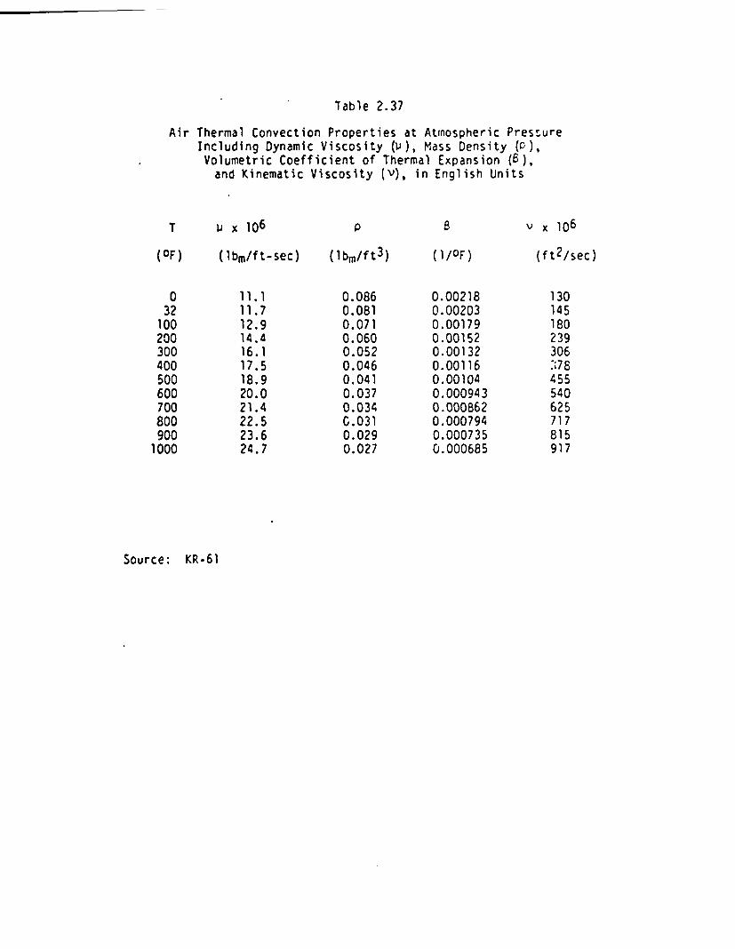
Table 2.37
Air Thermal Convection Properties at Atmospheric PressureIncluding Dynamic Viscosity (), Mass Density (),Volumetric Coefficient of Thermal Expansion (6),and Kinematic Viscosity (v), in English Units
T u x 106 p 8 v x 6
(OF) (lbm/ft-sec) (lbm/ft3) (1/OF) (ft2/sec)
0 11.1 0.086 0.00218 13032 11.7 0.081 0.00203 145100 12.9 0.071 0.00179 180200 14.4 0.060 0.00152 239300 16.1 0.052 0.00132 306400 17.5 0.046 0.00116 :;78500 18.9 0.041 0.00104 455600 20.0 0.037 0.000943 540700 21.4 0.034 0.000862 625800 22.5 C.031 0.000794 717900 23.6 0.029 0.000735 8151000 24.7 0.027 0.000685 917
Source: KR-61
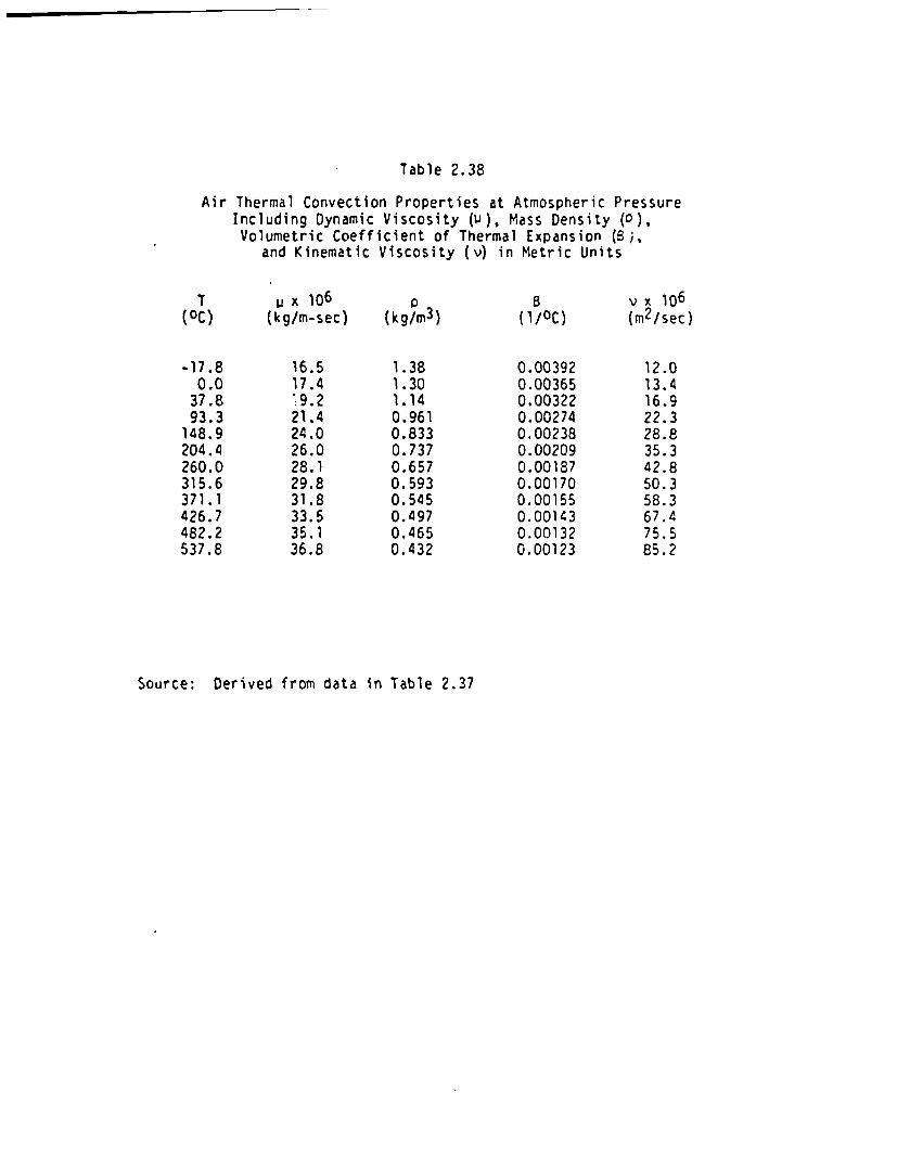
Table 2.38
Air Thermal Convection Properties at Atmospheric PressureIncluding Dynamic Viscosity (), Mass Density (),Volumetric Coefficient of Thermal Expansion (;,
and Kinematic Viscosity (v) in Metric Units
(0C)
-17.80.037.893.3148.9204.4260.0315.6371.1426.7482.2537.8
x 106(kg/m-sec)
16.517.4'.9. 221.424.026.028.129.831.833.535.136.8
P(kg/m3)
1.381.301.140.9610.8330.7370.6570.5930.5450.4970.4650.432
B(lf°C)
0.003920.003650.003220.002740.002380.002090.001870.001700.001550.001430.001320.00123
v x 106(m2 /sec)
12.013.416.922.328.835.342.850.358.367.475.585.2
Source: Derived from data in Table 2.37
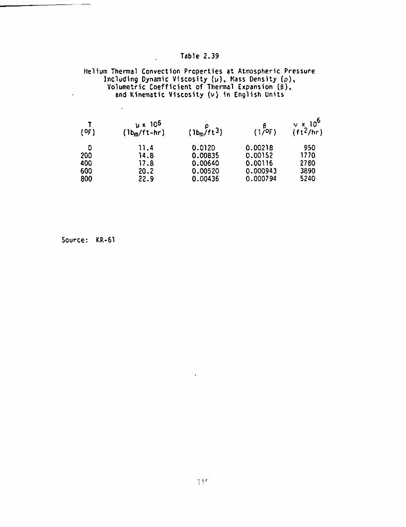
Table 2.39
Helium Thermal Convection Properties at Atmospheric PressureIncluding Dynamic Viscosity (), Mass Density (p),Volumetric Coefficient of Thermal Expansion ().
and Kinematic Viscosity (v) in English Units
T(OF)
0200400600800
X lo6(ibm/ft-hr)
11.414.817.820.222.9
P(lbm/ft 3 )
0.01200.008350.006400.005200.00436
6 v x lO6(1/OF) (ft2/hr)
0.002180.001520.001160.0009430.000794
9501770278038905240
Source: KR-61
1 Irr
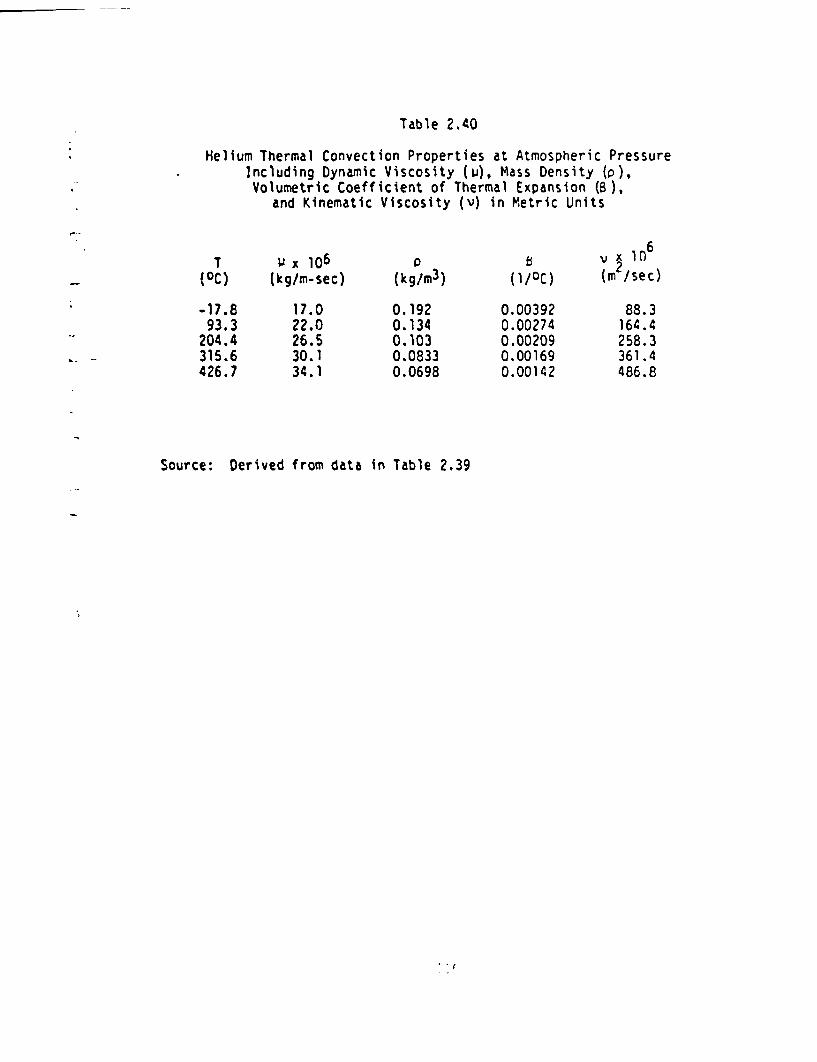
Table 2.40
Helium Thermal Convection Properties at Atmospheric PressureIncluding Dynamic Viscosity (), Mass Density (a),Volumetric Coefficient of Thermal Expansion (),
and Kinematic Viscosity (v) in Metric Units
T x 106 v X io6(0C) (kg/m-sec) (kg/m3) (m2C) (m /sec)
-17.8 17.0 0.192 0.00392 88.393.3 22.0 0.134 0.00274 164.4
204.4 26.5 0.103 0.00209 258.3315.6 30.1 0.0833 0.00169 361.4426.7 34.1 0.0698 0.00142 486.8
Source: Derived from data in Table 2.39

Table 2.41
Saturated Liquid Water Thermal Convection PropertiesIncluding Dynamic Viscosity (), Mass Density ()Volumetric Coefficient of Thermal Expansion (),
and Kinematic Viscosity (v) in English Units
T u x 103 p x 103 v x 1o6
(OF) (lbm/ft-sec) (lbm/ft3) (I/OF) (ft2/sec)
32 1.20 62.4 -0.04 19.350 0.880 62.4 0.05 14.0100 0.458 62.0 0.20 7.40150 0.292 61.2 0.31 4.77200 0.205 60.1 0.40 3.41250 0.158 58.8 0.48 2.69300 0.126 57.3 0.60 2.20350 0.105 55.6 0.69 1.89400 0.091 53.7 0.80 1.70450 0.080 51.6 0.90 1.55500 0.071 4'.0 1.00 1.45550 0.064 45.9 1.10 1.39600 0.058 42.4 1.20 1.37
Source: KR-61
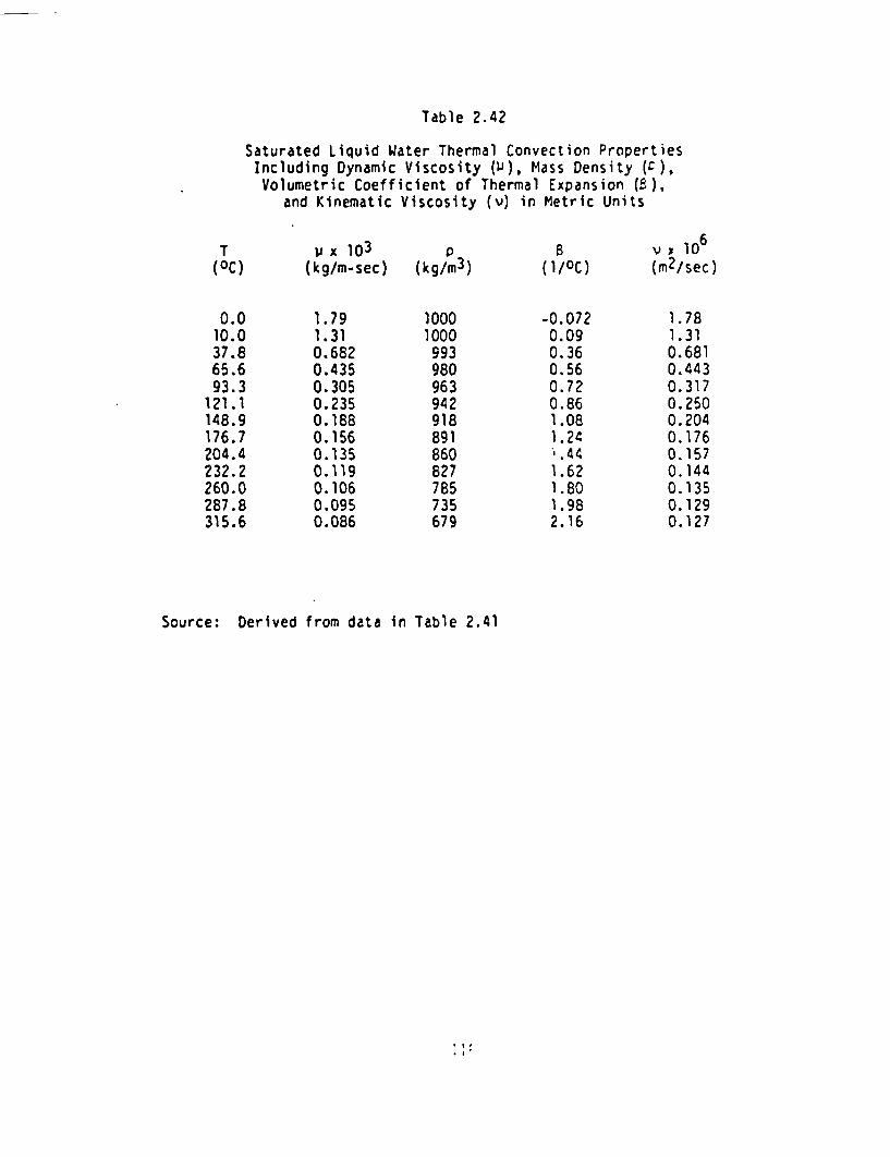
Table 2.42
Saturated Liquid Water Thermal Convection PropertiesIncluding Dynamic Viscosity (), Mass Density (),Volumetric Coefficient of Thermal Expansion (),
and Kinematic Viscosity (v) in Metric Units
T(0C)
0.010.037.865.693.3121.1148.9176.7204.4232.2260.0287.8315.6
x 103
(kg/m-sec)
1.791.310.6820.4350.3050.2350.1880.1560.1350.1190.1060.0950.086
(kg/m 3 )
10001000993980963942918891860827785735679
8( l / 0C)
-0.0720.090.360.560.720.861.081.24'.441.621 .801.982.16
V 106(m2/sec)
1.781.310.6810.44 30.3170.2500.2040.1760.1570. 1440.1350.1290.127
Source: Derived from data in Table 2.41
. I
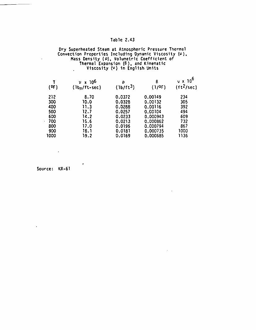
Table 2.43
Dry Superheated Steam at Atmospheric Pressure ThermalConvection Properties Including Dynamic Viscosity (i),
Mass Density (), Volumetric Coefficient ofThermal Expansion (), and Kinematic
Viscosity (v) in English Units
1 iix 1 6 P B v x 106(OF) (lbm/ft-sec) (lbIft3) (1/OF) (ft2/sec)
212 8.70 0.0372 0.00149 234300 10.0 0.0328 0.00132 305400 11.3 0.0288 0.00116 392500 12.7 0.0257 0.00104 494600 14.2 0.0233 0.000943 609700 15.6 0.0213 0.000862 732800 17.0 0.0196 0.000794 867900 18.1 0.0181 0.000735 10001000 19.2 0.0169 0.000685 1136
Source: KR-61
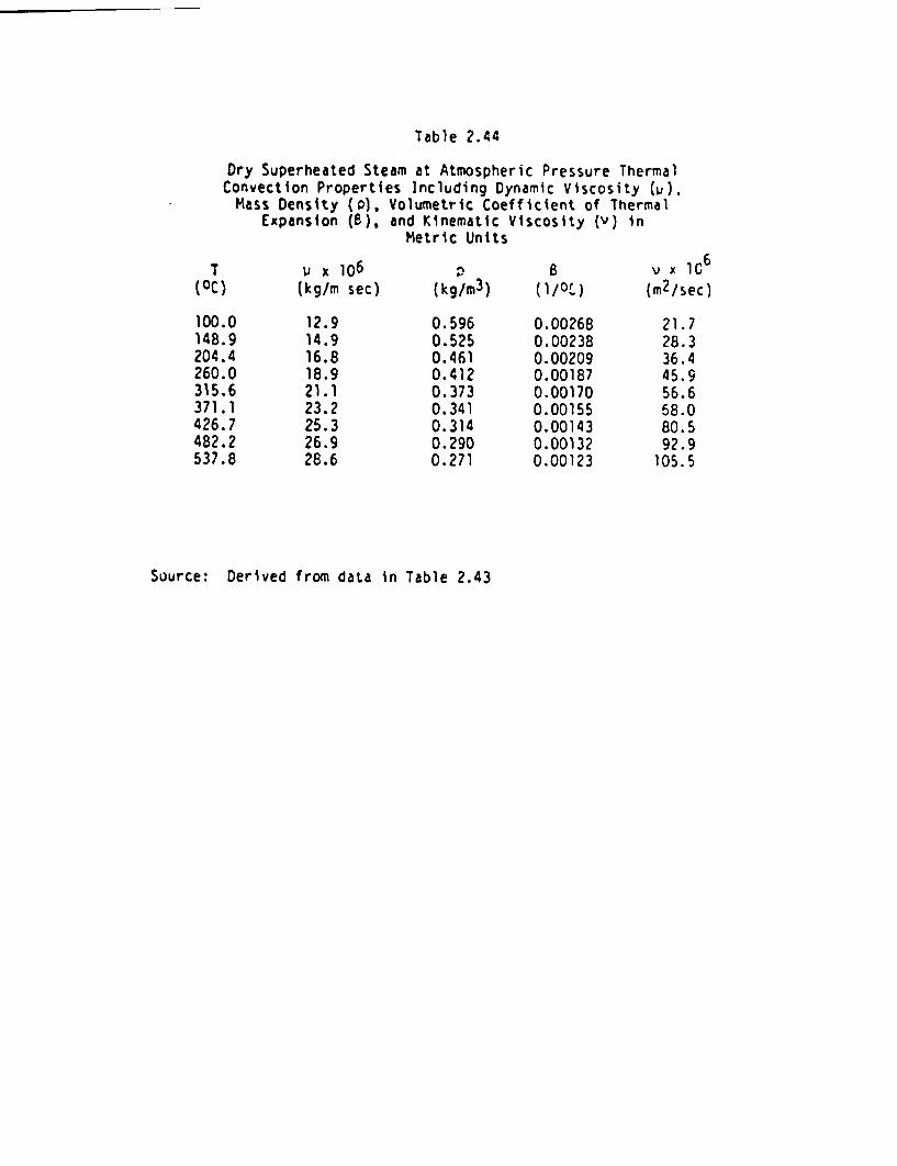
Table 2.44
T(0C
100148204260315371426482537
Dry Superheated SteamConvection PropertiesMass Density (), Vo'
Expansion (6), ani
u x 106) (kg/m sec)
.0 12.9
.9 14.9
.4 16.8
.0 18.9
.6 21.1
.1 23.2
.7 25.3
.2 26.9
.8 28.6
(kg/m3)
0.5960.5250.4610.4120.3730.3410.3140.2900.271
at Atmospheric Pressure ThermalIncluding Dynamic Viscosity ().lumetric Coefficient of ThermalI Kinematic Viscosity () inMetric Units
8
0.002680.002380.002090.001870.001700.001550.001430.001320.00123
v x 1C6
(m2 /sec)
21.728.336.445.956.658.080.592.9105.5
Source: Derived from data in Table 2.43
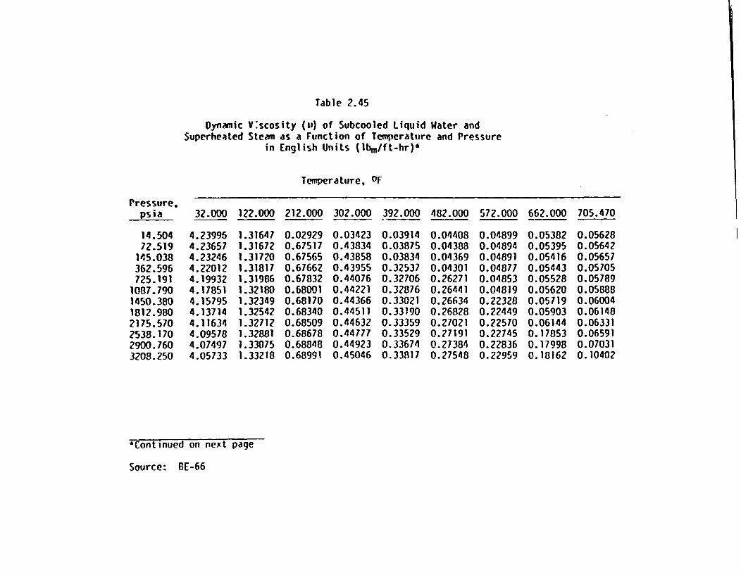
Table 2.45
Dynamic V:scosity () of Subcooled Liquid Water andSuperheated Steam as a Function of Temperature and Pressure
in English Units (bm/ft-hr)*
Temperature, OF
Pressure,psia
14.50472.519
145.038362.596725.191
1087.7901450.3801812.9802175.5702538.1702900.7603208.250
32.000 122.000 212.000 302.000 392.000 482.000 572.000 662.000 705.470
4.239964.236574.232464.220124.199324.178514.157954.137144.116344.095784.074974.05733
1.316471.316721.317201.318171.319861.321801.323491.325421.327121.328811.330751.33218
0.029290.675170.675650.676620.678320.680010.681700.683400.685090.686780.688480.68991
0.034230.438340.438580.439550.440760.442210.443660.445110.446320.44 7770.449230.45046
0.039140.038750.038340.325370.327060.328760.330210.331900.333590.335290.336740.33817
0.044080.043880.043690.043010.262710.264410.266340.268280.270210.271910.273840.27548
0.048990.048940.048910.048770.048530.048190.223280.224490.225700.227450.228360.22959
0.053820.053950.054160.054430.055280.056200.057190.059030.061440.178530.179980.18162
0.056280.056420.056570.057050.057890.058880.060040.061480.063310.065910.070310.10402
*Continued on next page
Source: BE-66

Table 2.45 (continued)
Temperature, OF
Pressure,psia 752.000 797.000 842.000 887.000 932.000 1022.000 1112.000 1202.000 1292.000
14.50472.519
145.038362.596725.191
1087.7901450.380181 .9802175.5702538.1702900.7603208.250
0.058830.058980.059120.059560.060360.061280.062320.063530.064980.066740.069060.07183
0.061300.061420.061570.061980.062750.0636C0.064540.065610.066840.068290.069980.07177
0.063770.063890.064010.064420.065150.06594C.066820.06778O.058870.070110.071510.07288
0.066210.066330.066480.066860.067540.068290.069110.070010.071000.072070.073270.07442
0.068680.068800.068920.069310.069960.070660.071440.072260.073180.074140.075210.07622
0.073610.073710.073830.074170.074800.075450.076130.076850.077650.078480.079370.08017
0.078520.078620.078740.079060.079640.080240.080870.081520.082220.082950.083720.08442
0.083460.083560.083650.083970.084500.085060.085640.086240.086870.087520.088220.08882
0.088370.088470.088560.088850.089360.089870.090430.090980.091560.092170.092800.09333
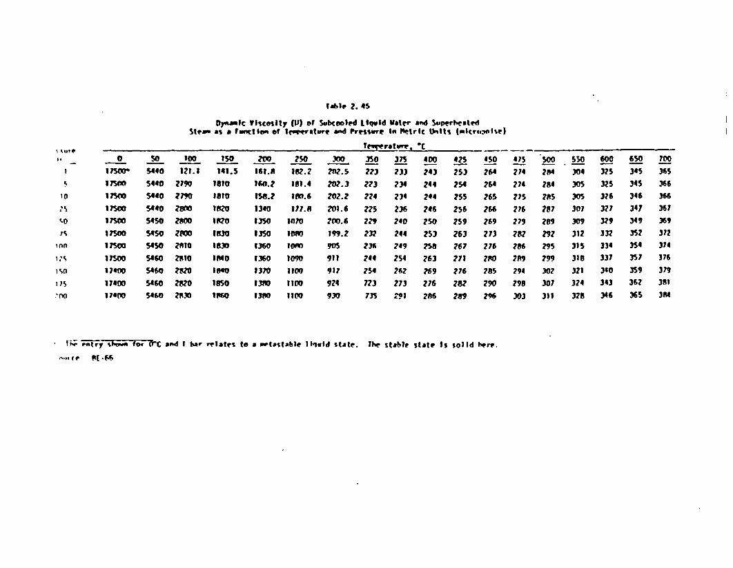
Table 2. 45
Oy mic VIscosity (PI) of Sobcooled liquid atew and Superbeatedtem as Function of Teoprature and Pressure Metric Units (micrts, e)
0,
I.
I0
s'
I WIf
175o
0
1 7500In00I MMo
17501700
1 JSO0
17400
17100
So too 150
5440 t2.1 141.5
5440 0 1no 8105440 7790 int
5440 710 157
S450 7800 1R20
S450 700M I50
S450 ZRIO 1830
5460 7810 1M0
5460 10 18
5460 M0 1850
5460 2830 lo0
00 250
161.8 187.2
160.2 181.4
158.? 180.6
1340 177.P
1350 1070
1350 T0M
1360 To
1360 1090
1370 300
1380 T1M138 VWO
72.5
M0. 3
202. 2
201.6
700.6
199.7
905911
917
924
930
Te"yre 'Cve
3SO 375 40223 233 24
223 234 24224 234 24225 236 241729 240 254232 244 25236 249 75244 254 6
254 267 76773 273 2773S I 781
D
3
II
5
3
3
IS
S
425
253
254
255
256
759
263
767
271
276
287
2J8
450
764
264
765
266
269
273
Z76
270
285
290
296
475 500 5i0 600274 284 304 375
274 784 305 3Z5
775 75 30S 376276 287 307 327279 289 309 32927 297 312 332286 295 315 3342P9 799 318 337294 302 321 340298 307 324 343
303 311 328 346
650
345
34S
346
347
349
35?
354
357
359
362
365
700
365
366
366
367
36,
372374
376
379381
3M
* yi Petry Sfwm for (c and I bar relates to a tostable loiqld state. The stable state is solid here.
-9( P Sf44
For water in the turbulent region NGr > 4 x 10⁸ where GrPr > 2 x 10⁹ .
Geidt (Reference G-60, indicates experimental data are well represented
by
Wu 0.17(GrPr)0 .33
(2.149)
h 0.17 (k/L) (GrPr)0 -33
(2.150)
where L is the vertical dimension.
2.2.2.4 Fluid Convection Properties
Fluid properties that are needed to evaluate convection correlation
terms include the fluid dynamic viscosity, , and the volumetric coef-
ficient of thermal expansion B. Data are presented in the following
tables for: air and helium at low pressures, saturated liquid water,
dry saturated steam, subcooled water, and superheated steam. The
specific volume tables for subcooled water and superheated steam that
were presented in Section 2.2.1 can be used to calculate using
v( )T P
(2.151)
2.2.3 Radiation Parameters
2.2.3.1 Stefan-Boltzmann Constant
The Stefan-Boltznann constant is:
C 0.1712 x 10⁻⁸ Btu/hr-ft2 _OR4
G = 1.355 x 10⁻¹² cal/sec-cm2 -OK4
0 5.67 x 0-8 W/m2-OK4
2.2.3.2 Emissivity Date
Table 2.48 presents surface emissivity data for various solid materials
of-interest in waste package design.
2.2.3.3 View Factors
For waste package analysis, the most frequently encountered geometry of
bodies between which radiation heat exchange occurs is expected to be
concentric cylinders. This is fortunate because, if the cylinders can
be treated as infinite in length (a treatment compatible with the vast
majority of one-dimensional conduction analyses), the view factor for
the smaller cylinder is unity. This assumes there is no absorbing
medium between the surfaces such as a gas or that the medium has a
negligible effect if it is present.
Analysts who encounter other geometric configurations between which
radiative heat transfer is occurring can use Euation 2.52 and Figure
2.5 to evaluate the view factor by performing the double integral. Text-
books sometimes graphically quantify the view factors for some geometric
configurations. The possibilities are unlimited, and particular ones
are not presented here.

Table 2.48
Values of Surface Emissivityfor Solid Materials
T(OF)
Cast Iron
recently machined 72machined and heated 1620machined and heated 1810smooth, oxidized 130smooth, oxidized 520
Carbon Steel
oxidized steel 390oxidized steel 1100
Stainless Steel
304-42 hrs at 5300F 220polished 100
C
0.440.60.70.780.82
0.790.79
0.620.13
Sources: GI-61, oxidized steel, smooth oxidized cast ironBA-77, 304-42 hrs at 5300F
polished stainless steelHO-81, machined cast iron, machined and heated cast iron

3.0 STRUCTURAL MECHANICS
3.1 Analytical Techniques
3.1.1 Objectives of Analysis
The purpose of analytical structural mechanics, as it relates to waste
package performance, is to evaluate conditions in a constrained structure
when expected service loads act on it. The conditions are monitored as
responses, such as displacements, deformations, strains, and stresses.
Mechanical analysis is performed and structural conditions are monitored
to facilitate evaluation of the responses for all the anticipated loading
cases against responses that have been found to allow acceptable service
for the life of the structure.
3.1.2 Structural Analysis Approaches
Structural analysis tends to follow one of two approaches. The first
approach is the use of formulas which typically are solutions to contin-
uous differential equations. These formulas are usually taken from
strength of materials, mechanics of materials, and theory of elasticity
texts for structures whose geometry, loading, constraints and material
properties are well defined. Formulas are available for most problems
that can be solved analytically with reasonable resources. The formulas
are precise analytical solutions that aid in the understanding of mechanics
and complement information gained experimentally. The formulas should
be used only for conditions similar to the analytical problem that was
solved when the solutions were derived. The proper application of formu-
las is instructive, straightforward, and reliable. However, for complex
problems analytical solutions are often not available.

The second method of analysis is the use of finite increment techniques
including finite element and finite difference methods. The use of
finite increment methods requires specifying a structure as an assem-
blage of discrete interactive parts. This simplification in problem
formulation reduces the differential equations describing structural
response to algebraic equations and allows analysis of more intricate
structures than does the "formula" method. These finite increment methods
are usually applied using a computer and computer program to order and
automate the solution procedure. Such programs typically solve a set of
coupled algebraic equations for the displacement of points (nodes) whose
coordinates are defined for the structure before application of the
loads. The equations are coupled because the nodes are connected to
various other nodes by elements with particular stiffness character-
istics. By specifying the stiffness characteristics of each element of
the constrained structure and applying displacement compatibility of
elements and force equilibrium at a common node; one can evaluate the
deflection of nodes; deformation of structural elements between nodes;
the forces and strains in structural elements at various nodes; and
finally the stresses in the elements. Adjacent elements with hetero-
geneous characteristics such as different materials can be represented.
This is in contrast to the differential equations which are applicable
to a continuum. Thus, the finite increment methods are very adaptable
to solving actual problems. This adiptation irvnIves up-front simpli-
fications yielding sets of algebraic equations that can be solved using
computer methods. Finite increment methods can generally be applied
successfully to most simple and complex engineering mechanics problems.
3.2 Mechanics Principles
3.2.1 Displacement, Deformation and Strain
It is desirable that a structure carry the imposed loading conditions
envisioned during its service life without incurring significant dis-
tortions. This is necessary to maintain stability and to maintain
tolerances with interfacing equipment. Also, the design of the struc-
ture must be adequate to prevent structural failure.
Distortion causes common structural materiAls such as steel to lose
ductility.* If large distortions occur, the material may become
brittle in local regions and fracture. Theories of failure have been
developed for various classes of materials but ductile structural metals
such as steels usually experience shear failure when loaded excessively.
Shear failure is described in Appendix C (see the Tresca criterion).
Limiting deformation is the most direct means of preventing structural
failure.
Many conditions must be specified in order to perform this analysis of a
structure. One must specify the location of the structure in space.
Geometric deformation conditions due to loading are described in terms
of the displacements u, v, and w along the Cartesian coordinates x, y,
and z or r, 6, z along the polar coordinates at a general point in the
structure.
*Ductiity is the capability of the material to deform without crackingor rupturing. A brittle material is one that has very little ductility.For example, soft copper is a ductile material, while glass has verylittle ductility.
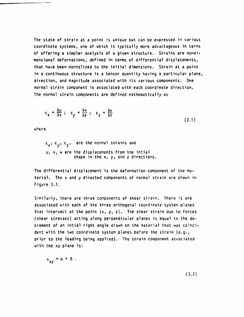
-
The state of strain at a point is unique but can be expressed in various
coordinate systems, one of which is typically more advantageous in terms
of offering a simpler analysis of a given structure. Strains are nondi-
mensional deformations, defined in terms of differential displacements,
that have been normalized to the initial dimensions. Strain at a point
in a continuous structure is a tensor quantity having a particular plane,
direction, and magnitude associated with its various components. One
normal strain component is associated with each coordinate direction.
The normal strain components are defined mathematically as
C~s ax; Cy ay; C = az(3.1)
where
Ex Cy X cz are the normal strains and
u, v, w are the displacements from the intialshape in the x, y, and z directions.
The differential displacement is the deformation component of the ma-
terial. The x and y directed components of normal strain are shown in
Figure 3.1.
Similarly, there are three components of shear strain. There is one
associated with each of the three orthogonal coordinate system planes
that intersect at the point (x, y, z). The shear strain due to forces
.(shear stresses) acting along perpendicular planes is equal to the de-
crement of an intial right angle drawn on the material that was coinci-
dent with the two coordinate system planes before the strain (e.g.,
prior to the loading being applied). The strain component associated
with the xy plane is:
er
(3.2)

u II
C I
A
A u.c.
AV
0
B
v
v *AV A - vA% y
..- X -UAx
(: limX Ax
x -x
AX
( limY
-U-
y y
x0B
I u. u AI
a) Pure normal strainstresses) cting in x
in x direction and in y direction due to forces (axialand in y directions
y
L
C
- u
A
- u
xy a -
IYxy = 'au .
a u a vaY-ay * x
Vx
Jim bAx
V . AVV
I 4 B I
0
b) Pure strain in x - y plane due to forces (shear stresses) acting alon x zand y - z planes
Figure 3.1
Stroin Companents Related Geometricolly to Displocements

Figure 3.1 shows how shear strain components are related geometrically
to displacements.
The three shear strain components can be written in terms of the dis-
placements as
'Y u rv au'+ aYxy a y ax Yyz a + Wy; Yz= a + axWaz By x (az ax
(3.3)
where
'YxksYyz, Yxz shear strains
u, v, w displacements from the initial shape to thestrained state in the x, y, and z directions,respectively.
The strain matrix consists of six strain components with potentially
unique magnitudes and is used with sign conventions to describe the
state of strain at a point. In matrix form, the strain is defined in
terms of the component magnitudes as:
CxE'Y xy
1.2 Yxz
C 17 'Yxy y
12~ Yyz
17 Yxz
1Yyz
cz
(3.4)
The matrix elements denote the magnitudes of strains. Both the magnitude
and direction of the strains are shown in Figure 3.1.
I

Principal strains at a point in the structure are the normal strains
occurring along a set of coordinates which are normal to a set of three
intersecting orthogonal planes on which there is no shear strain. These
planes will remain fixed in space as strains are induced. The normal
vectors may change magnitude but not direction. These planes are the
principal planes, and the normals are the principal directions. The
strains in the principal directions are principal strains. Mohr's dia-
grams for principal strains are discussed in Appendix B. The principal
strains cl, c2, and £3 are the three real roots of the equation
3 - IC 2 £ + C IC, - °-
(3.5)
whEre the coefficients Irl, 1c2, and 1c3 are the strain invariants:
Cl 2CX Ey C CZ Cl + 2 + C3
(3.6)
L 2 2
X C + CC 2 ~Y z c~c +C c *c3+clr2 xy yz xz 4 _ 4 1? 23 13
(3.7)
I2 C-2 Y2 Y
£3 CXECYZ 4 - 4 ' 4 + y4 Y1 XZ ClC2C3
(3.8)
The first strain invariant is equal to the volumetric strain and is
often referred to as the dilation. The notation is:
A 6V 9)V Cl
(3.9)

where
A volumetric strain
V = original volume
6V change in volume.
'The direction cosines of the principal plane (, m, and n) with respect
to an arbitrary plane, -, are given by
2 = + (a -c2) (c 3)
(C1 -C2 ) ( 1 -C 3 ) (3.10)
m2 ) ( (c7 -c2) (T-C3)
(C2-C 3 ) ( 2 -c 1 ) (3.11)
(,r2
2 (2 (Cr-Cl) ( c2)n
(C3-CL) ( 3-c2)
(3.12)
where Y. and C', are the shear strain and normal strain for plane .The Mohr diagram methods discussed in Appendix B are used to determine
the principal strains and their directions.
To aid in envisioning and handling the strain tensor, it is conceptual-ized in two parts: a spherical part and a deviator part. The spherical
part is:
slit S 0 ^ 0
S O O
] 4.

where sj is the spherical strain tensor and represents a dilation (or
shrinking) of the original geometry with an associated change in volume.
The deviator strain is given by
= ~ Yxy
17 'Yxz
I IEYxy T Yxz
3 1c ~ 2Yz
ex 2 Yxy
1T JYxy ey
_-2 x yz
2 yz
eZ -
2 1~ Y xzI
I.-. Yyz 3-
(3.14)
whEre
dij deviatoric strain
ex, ey e deviatoric strain components
A mean strain.
The deviatoric strain tensor represents a change in shape without any
change in volume. Failure in structural metals is closely related to
the state of deviatoric strain and relatively independent of the spheri-
cal strain. Deviatoric strain invariants exist but are not comronly
used and thus not included here.
The maximum shear strains are given by:
Y ' C12 t3l(3.15)
Y2 Icl - 31
(3.16)
I -,I

-Y3 jl 21
(3.17)
The largest of the three maximum shear strains is the key index of fail-
ure for ductile metals.
For some types of analyses,
strain rates are used. The
particularly those dealing with energy methods,
strain rates are defined as:
axx ax'=
. ay ay az
(3.18)
avX av~xY -y + .ixy ay axe
i Cav avZyZ z ;y
i avx avxX2 az ax
(3.19)
where
Cx, Cy, CZ normal axial strain rate components
Yxyt YyzI xz shear strain rate components
vx, vy, vz time rate of displacement in x, y, and zdirections respectively.
All of the preceding relationships given for strains are equally valid
for strain rates. Strain rate tensors, deviatoric strain rates, strain
rate invariants, principal strain rates, and principal shear strain
rates are used in various relationships.
I .
In 1828, Poisson studied materlal behavior and found that the ratio of
the magnitude of strain in a lateral direction (in which there is no
applied load) to that in the direction coincident with uniaxial loading
vayles with material type. When a tensile load is applied, there is an
elongation strain (conventionally positive) n the loading direction and
a contraction strain (conventionally negative) in each of two directions
which are orthogonal to the loading direction and mutually orthogonal.
The Poisson ratio is defined as
.lateral strain)-axial strain
(3.20)
and is a property of a material.
3.2.2 Internal Loads and Stresses
Loads, ncluding forces and moments, are transmitted internally through-
out a structure. both uniform and nonuniform forces act over a cross-
sectional area due to these internal loads. It is often necessary to
determine the local loading due to its variation with position. Ultimately,
loads must be compared to the load-carrying ability of the material so
that conclusions regarding structural adequacy can be made. The structural
load and the material's load-carrying capability are specified on a uni-
form force per unit area basis. This quantity is called stress or allow-
able stress for the material. Stress is a convenient basis for judging
structural adequacy of low-performance structures (those subject to
short term loading, room temperature, and no plastic deformation).
Because internal loads in a cross section vary with position, it is nec-
essary to base the stress on a very small area at a point in the cross
section, which can be compared to the material allowable stress. There-
fore, the definition of normal stress component is

1 . imit IFx A 0 (
(3.21)
where
F net traction load on area A in the x direction [f]
2A cross-sectional area El I
ax stress component in x direction 2(tensile stress is conventionally If/2 )positive)
This equation is typically written
Fx
x A(3.22)
where
Fx = axial force in x direction [f]
A = area in yz plane of cross section )r2]
It is understood that the force on a small local area must be considered
if a nonuniform load distribution is present. The gross cross-sectional
quantities can be used if the force is uniformly distributed over the
area.
Any force acting on the plane of the cross section can be specified in
terms of two orthogonal forces, F and F, acting on one of the faces
parallel to the y-z r ne. In general, these forces vary with position
over the cross section and are specified for the local infinitesimal
area at a point to give the following shear stress components at that
point:
limit ( i
xy A - 0 ~~~~~~~~~~i ~(3.23)
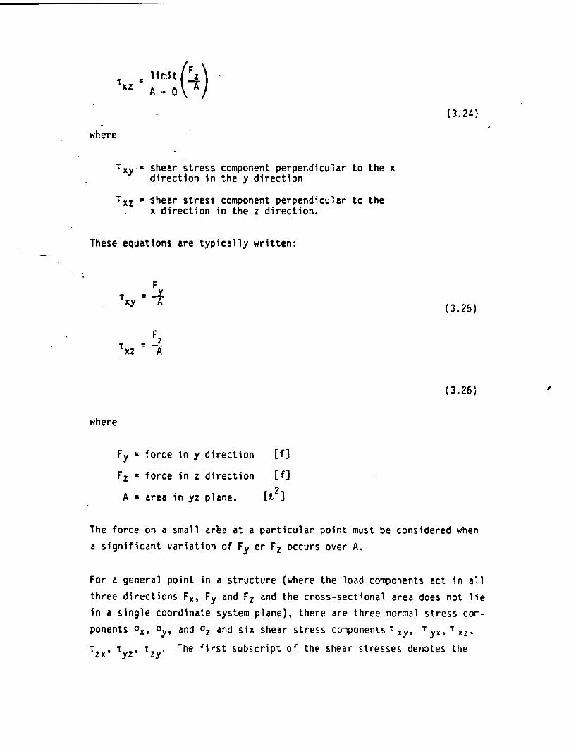
T , limitxz A-
(3.24)
where
Txy-= shear stress component perpendicular to the xdirection in the y direction
xz r shear stress component perpendicular to thex direction in the z direction.
These equations are typically written:
F
xy A(3.25)
I2
(3.26) be
where
Fy = force in y
F2 force in z
direction
direction
[f)
If]23
A area in yz plane.
The force on a small area at a particular point must be considered when
a significant variation of F or F occurs over A.
For a general point in a structure (where the load components act in all
three directions Fx, F and Fz and the cross-sectional area does not lie
in a single coordinate system plane), there are three normal stress com-
ponents Ox y and 0z and six shear stress components xy, T yx Txzo
Tx, Tyk T. The first subscript of the shear stresses denotes the

axis to which the stress is normal and the second the direction of theassociated force component causing the stress. Because of the different
directions of the shear stresses, in general, the vectors:
TXY YZ
Txz TzX
T Tyz zy
(3.27)
The Taj are tensor components that act on different planes and havedifferent directions. The differences in the Txy and TXy components canbe investigated for a body acted upon by pure shear as shown in Figure3.2. Moment equilibrium can be applied at point 0 about the z axis:
(+EM' 0 O [r IYI (xbz)by - IT Iy (yaz)bx
(3.28)
which indicates
IT I TXT I(3.29)
which
for
means the two components have equal magnitudes. This is also true
ITYZ I = ITZYI
(3.30)
140
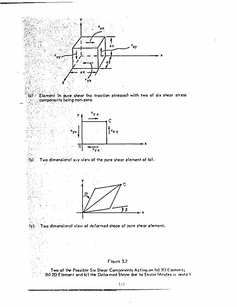
AI~~~~~~~~v~A
.t ,\'*f. R '
1~~ xA
(o) Elermntln pure shear Cn otraction stresses) with two of six shear stresscompot ts being non-zero
yx~~~tx
?yX ~ ~ ~ ~~
b) Two dlimensi6oal xy vie of the pure sheor element of (1
V
.4~~~~~~~~c
Two .1~,dimensoneol viev., of deformed shape of pvre shear element.
Fiqvre 3.2
Two of the Passible Six Shear Components Actinq on () 31) F.ement;(h 7D Element and e) the Deformed Shope s i to Strain (Angrles a ci I
- , . . -components being nor!-zero~~~~~~~~~~

y
yx
fIxy
Ay- T /_ - x
z ryx
Element in pure shear (no roction stresses} with two of six shear stresscomponents being non-zero
()
y IyX
C
TX y
_ 1* x0
'yx
(b) Two dimensional x-y view of the pure shear element of ().
y
x
fc) Two dimens;onnt vew of deformed shape of pure shear element.
Fiqure 3.2
Two of the Possible Six Sear Components Actinx on n) 31) lement;(b) ?D Flemrnet nnd (c) th- Deformed Shope de to Strnin (Arnie ( ncio, )
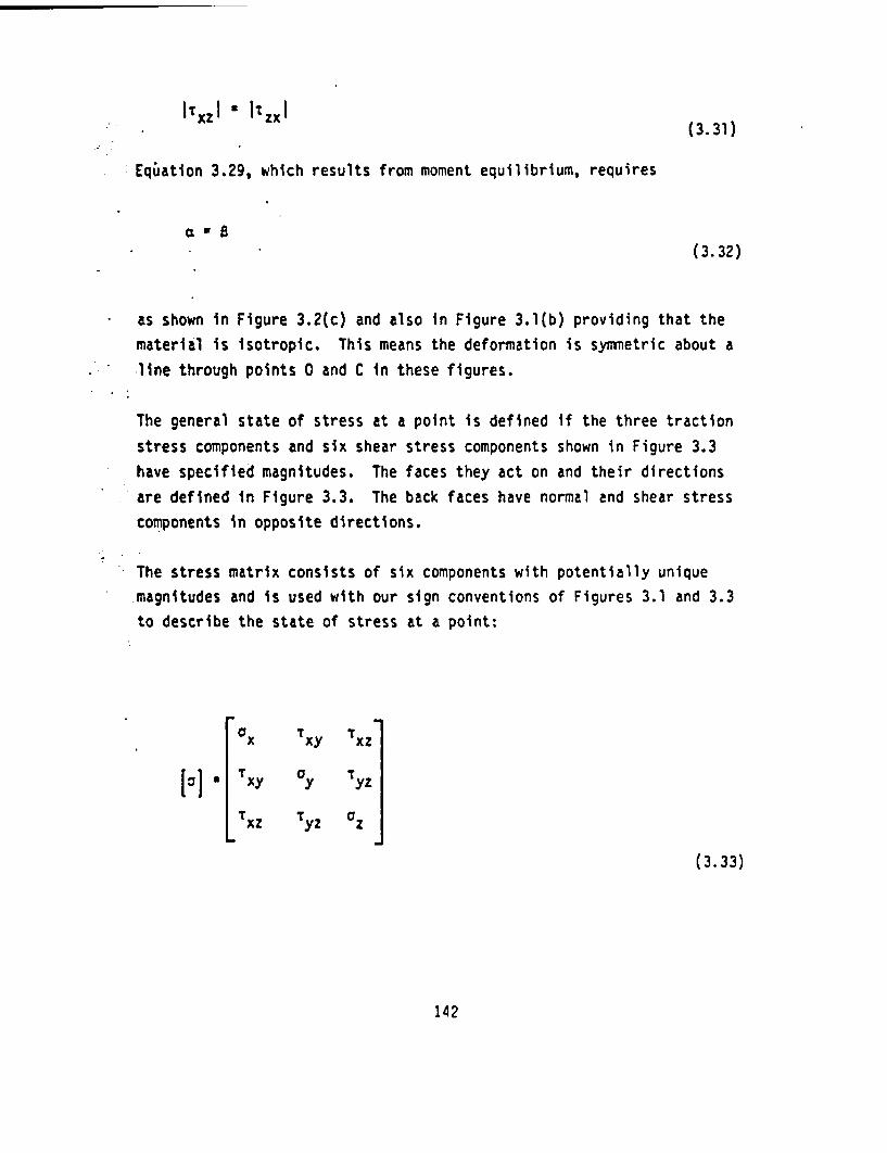
I rV7, IrYj(3.31)
Equation 3.29, which results from moment equilibrium, requires
ca B(3.32)
as shown in Figure 3.2(c) and also in Figure 3.1(b) providing that the
material is isotropic. This means the deformation is symmetric about a
line through points 0 and C in these figures.
The general state of stress at a point is defined if the three traction
stress components and six shear stress components shown in Figure 3.3
have specified magnitudes. The faces they act on and their directions
are defined in Figure 3.3. The back faces have normal and shear stress
components in opposite directions.
The stress matrix consists of six components with potentially unique
magnitudes and is used with our sign conventions of Figures 3.1 and 3.3
to describe the state of stress at a point:
x xy xz
Ia] T xy Cy 1 yz
Txz Tyz z
(3.33)
142
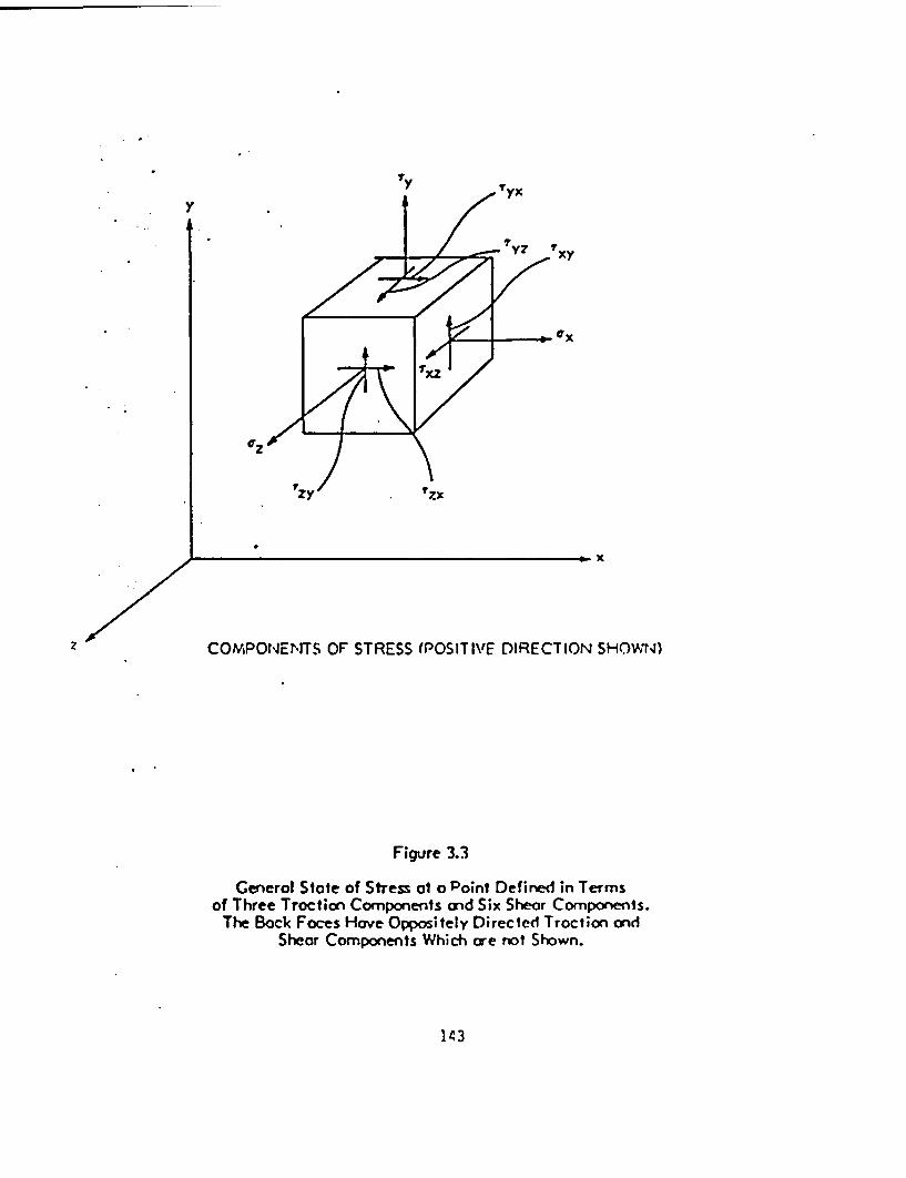
yI
W 7 y
T*Y?7 xy
Z/
7z
Tx2
- ex
Irz AI:011
tzx
x
z COMPONENPITS OF STRESS (POSITI\E DIRECTION SHOWN)
Figure 3.3
General State of Stress of a Point Defined in Termsof Three Traction Components and Six Shear Components.
The Back Faces Have Oppositely Directed Troction andShear Components Which oe not Shown.

where
ox a ox = traction stress components(negative if compressive)
keys TyZ, TXZ shear stress components.
Principal stresses at a point in the structure are the traction (orcompression) stresses occurring along a set of coordinates which arenormal to a set of three mutually orthogonal planes on each of whichthere s no shear stress. The principal stresses occur normal to theprincipal planes and are coincident with principal strains. A set ofprincipal stresses can be found for any generalized state of stress.The Mohr diagram method presented in Appendix B illustrates the processgraphically.
The principal stresses ,
equation
c2, and 03 are the three real roots of the
S3 I S2 + I S - I O 0
(3.34)
where
It a ax + °y +
(3. 35)
2 xY + Yy + xCZ T xy - T2 T2yz xz
(3.36)
13 a aaa + 2T T T _ a T2 _ a T2 a I23 xy yz x yz y xz z xy
(3. 37)
144
For a particular state of stress, the coefficients in Equation 3.34 are
related to a unique set of principal planes and are independent of the
initial coordinate system used to specify the structure's geometry and
loading. The coefficients are known as the stress invariants and can be
defined in terms of the principal stress components as
113°1+02+03
(3.38)
12 3 0102 + 0203 + 0103
(3.39)
13 00T203
(3.40)
To aid in envisioning and handling the stress tensor, it is conceptual-
ized in two parts: a mean part and a derivatoric part. The mean stress
cm is defined as:
am (a + 2 a3) 3 (x + y + aZ)
(3.41)
The mean stress, also known as the spherical stress, is independent of
-direction. For the special case of
ax ay z a m
(3.42)
145

the mean stress is defined as the hydrostatic stress. Physically the
hydrostatic state of stress has very little influence on failure. The
spherical stress tensor is written
an
0
0 0
Sij* a mi 0
0 0 am(3.43)
where
6ij is the Kronecker delta ordefined by 6ij 0 forfor i j
substitution tensori j and 6ij
The stress deviator tensor is given by
Di; t Oij Sij
(3.44)
or
Dij K
ax "m
Xyz
TzX
Txy
0 - aay a
TZY
.rxz
yz
0z mL
(3.45)
The hydrostatic stress deviator tensor in terms of the principal stress
is
a - rl O OD ~ ~ ' 0 0 0
Ojt 0 02 -' 0m
0 0 a -3 °m(3.46)
or from Equation 3.45
S* Tx xy xz
D~~~~ ~ SX *% TX
ij YX ~y yz
S*zx zy z
(3.47)
where Sx*, Sy and S are the deviatoric stress components.
Since any state of stress in general has invariants, the deviatoric
stress tensor can be shown to have invariants defined as
J1 S + S + S 0
(3.48)
J2 37E (Sx + Sy + S2 + 2 2 + 2T 2 + 2 T 2)2 7 x y z xy yz xz(
(S 2 2 + S 2)
(3.49)
147

SX i Ix
. 3 ITx S Iyz * /3 (S 3 S3 S 3)3 3
Txz IA Sz
(3.50)
where S, S2, S3 are the principal deviatoric stress components.
Parameters formulated in terms of the stress invariants are used to
indicate stress conditions in a structure. Their values are compared to
experimentally determined values at failure for the same material type
to judge structural adequacy. For example, the octahedral normal and
octahedral shear stresses are defined as :
Coct " 1 + 2 3)3 o(3.51)
TOct = > (S 12 +52 *S 3
2 )
where
Coct octahedral normal stress
a* 3
(3.52)
Toct octahedral shear stress.
These stresses act on a plane intersecting the principal axes at equal
angles. The name of these stresses derives from the fact that the plane
surface makes up one-eighth of a regular octahedron about the origin.
The maximum shear stress is a very important quantity as it is a direct
index to the failure of ductile materials. It is given by
148

TMax a aX (TA. e' TC)
(3.53)
where TA, s, and TC are the maximum shear stress on a two-dimensionalbasis
TA 2 102 el
B8 'IE103 lI
T 2 1 1° l
(3.54)
and where l, 2, and 3 are the principal stresses.
The maximum shear stresses on a two-dimensional basis, TA, T, and
T occur on planes that are at 450 to the principal stress directions
determined on a two-dimensional basis.
3.2.3 Constitutive Relationships
3.2.3.1 Types of Constitutive Relationships and Their Uses
Constitutive relationships are mathematical expressions that describe
the essence of the primary physical interaction that occurs in a solid
body or structure. The relationship is between the response expressed
in terms of strain and the stresses that are a direct consequence of the
internal loads carried by the structure.

The constitutive relationship is the most basic relationship between the
variables in a structural analysis method as it describes the fundamen-
tal cause-effect relationship between internal loading per unit area
(stress) and the response stated in terms of strain. The relationship
is defined in mathematical form and contains parameters whose values
pertain to a particular material type. The relationship is usually
limited to a particular category of strain. These strain categories are
typically:
* Instantaneous linear elastic
* Instantaneous plastic
* Long-term creep
The first two strain categories are instantaneous effects; the third is
cumulative over the time of loading. The third method can produce cumu-
lative strains over time along with the instantaneous strains from either
of the first two categories. Generally, creep strain increases with
higher stress levels and higher material temperatures.
When a tensile specimen fails, the failure for the material is reported
in terms of either reduction of area at the point of failure or elonga-
tion per unit length in one of several standard gauge length sections in
which the failure occurred. These data are closely related -to strain.
Strain is a more general index from which to judge structural adequacy
than is stress. If structural service is such that the instantaneous
response is in the linear elastic or plastic range and the loading dura-
tion is short and temperatures not excessive (about 30 years and 7000F
is acceptable for many structural steels), then creep strain contribu-
tions to failure can be neglected. When time of loading and/or tempera-
ture values are high, neglecting the creep strain can lead to faulty
conclusions regarding structural adequacy. Both instantaneous and creep
strains cause the ductility of the material to be consumed. Since the
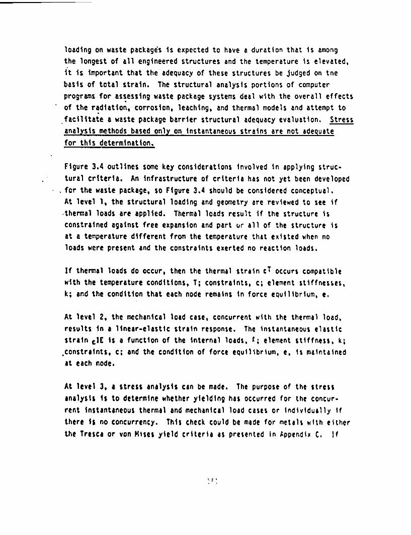
loading on waste packages is expected to have a duration that is among
the longest of all engineered structures and the temperature is elevated,
it is important that the adequacy of these structures be judged on tne
basis of total strain. The structural analysis portions of computer
programs for assessing waste package systems deal with the overall effects
of the radiation, corrosion, leaching, and thermal models and attempt to
facilitate a waste package barrier structural adequacy evaluation. Stress
analysis methods based only on instantaneous strains are not adequate
for this determination.
Figure 3.4 outlines some key considerations involved in applying struc-
tural criteria. An infrastructure of criteria has not yet been developed
for the waste package, so Figure 3.4 should be considered conceptual.
At level , the structural loading and geometry are reviewed to see if
*thermal loads are applied. Thermal loads result if the structure is
constrained against free expansion and part r all of the structure is
at a temperature different from the temperature that existed when no
loads were present and the constraints exerted no reaction loads.
If thermal loads do occur, then the thermal strain ct occurs compatible
with the temperature conditions, T; constraints, c; element stiffnesses,
k; and the condition that each node remains in force equilibrium, e.
At level 2, the mechanical load case, concurrent with the thermal load,
results in a linear-elastic strain response. The instantaneous elastic
strain CE is a function of the internal loads, ; element stiffness, k;
.constraints, c; and the condition of force equilibrium, e, is maintained
at each node.
At level 3, a stress analysis can be made. The purpose of the stress
analysis is to determine whether yielding has occurred for the concur-
rent instantaneous thermal and mechanical load cases or ndividually if
there is no concurrency. This check could be made for metals with either
the Tresca or von Mises yield criteria as presented In Appendix C. If
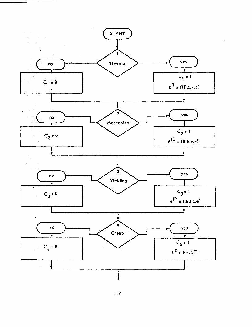
15?

5
f T C fTIC f C Ip, C3 1e C 2c C 3 4
Figure 3.4
Conceptual Structurol Criteria Application Procedure

yielding has not occurred and creep effects are known to be negligible,
a stress analysis may be adequate as an overall structural analysis
approach. If plastic deformation has occurred, strain limits are appro-
priate and best suited to judging structural adequacy. For a yielded
structure, the instantaneous plastic strain clP can be evaluated for
ductile metals using the Prandtl-Reuss equations with the von Mises yield
criterion. The procedure is similar to evaluating the instantaneous
elastic strain cIE except that the loads are applied incrementally and
summed for the entire loading.
For cases where loads are of long duration, temperatures are elevated,
and stress levels are high, the creep strain can be significant in com-
parison to the instantaneous strains. Creep strains tend to consume the
ductility of metals and cause metals to approach failure. When a struc-
ture may be susceptible to creep, rational design requires the creep
strain be evaluated (or estimated). This is typically accomplished by
using a correlation for creep strain, cc, with the state of stress, ;
time duration of loading, t; and temperature T as independent parameters.
After the instantaneous strains are evaluated at levels 1, 2, and 3 and
the creep strain is evaluated at level 4 for particular concurrent thermal
and mechanical load cases, the total strain can be evaluated at level 5.
At level 6, the design adequacy is evaluated by comparison to allowable
strain values. The strains resulting from various load set combinations
should be superimposed to obtain the response to all concurrent loading.
Strains should be categorized as membrane or bending stress and individual
limits imposed. To evaluate waste package performance, criteria need
to be defined for the various strain categories.
3.2.3.2 Generalized Linear Elastic Mechanical and ThermalConstitutive Relationship
In 1678, Robert Hooke published a linear constitutive relationship for
elastic materials when loaded in tension. This constitutive relationship
154
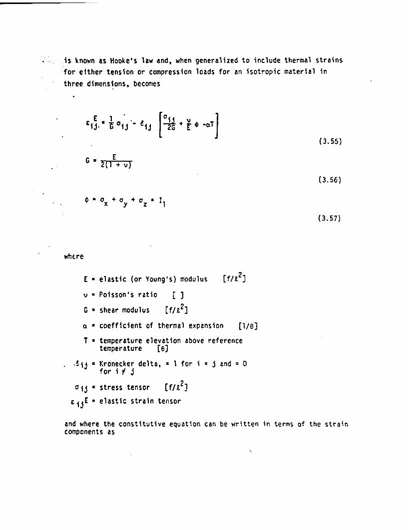
* is known as Hooke's law nd, when generalized to include thermal strains
for either tension or compression loads for an isotropic material in
three dimensions, becomes
E4-t:1-1 [ + -T]V i.U 1ij' ~ij T
(3. 55)
E2(1 + v)
(3.56)
¢ X+ a + zIx y z
(3.57)
whe-re
E elastic (or Young's) modulus [f/l 3
v Poisson's ratio [
G = shear modulus [f/Rt 2)
a acoefficient of thermal expansion [l/e]
T temperature elevation above referencetemperature [e)
iij a Kronecker delta, = 1 for i j and = 0for f J
°1 a stress tensor [f/Z2
C1 JE - elastic strain tensor
and where the constitutive equation can be written in terms of the straincomponents as
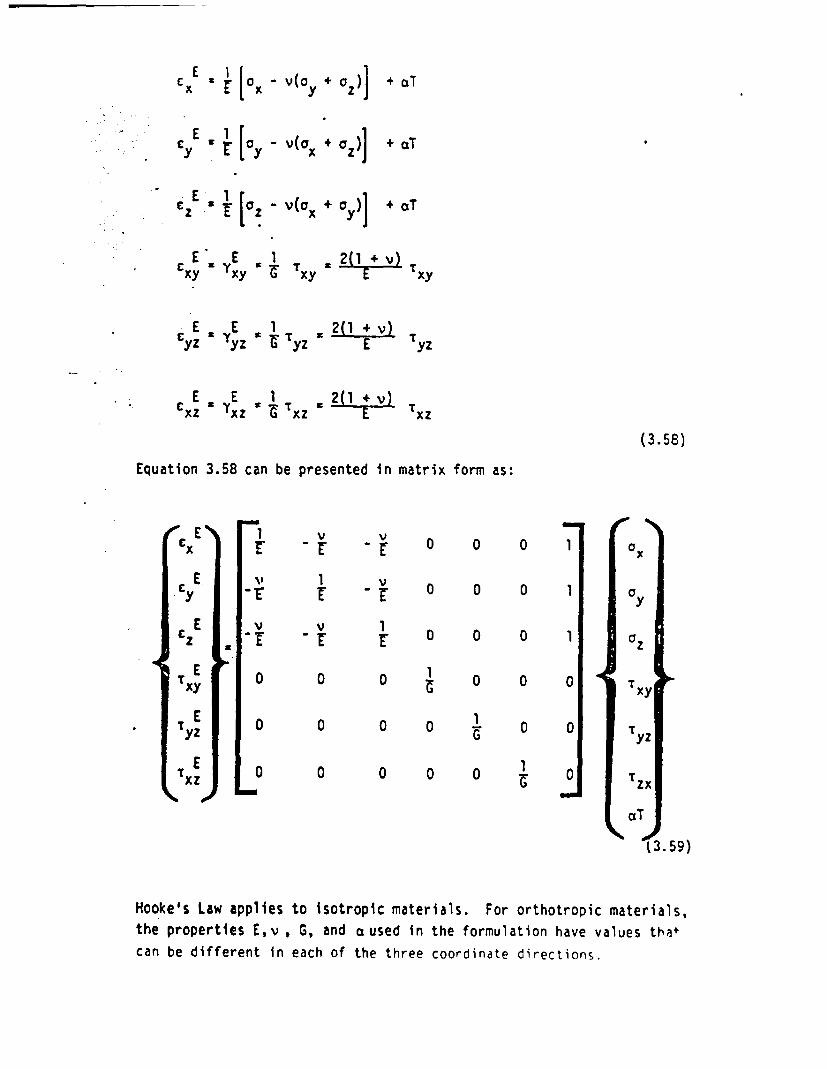
-
x
E
Cy
ECxy
ECyz
X [ - V(o .
F [ay -
z [o1 - V
E
E 1
a YX 6 X
' a)]
a)]
+ aT
+ T
+ ay)] aT
E Txy
Tyz
Tx ZE a YE E 1 t 2Cxz ~xz T x
(3.58)
Equation 3.58 can be presented n matrix form as:
.14
cxE
E
C E
ETxy
I E
XXZ
.I-1
r
-
0
0
0
-V - 0 0 0F -
1 v I -V 0 0 0
V 1-r1 0 0 0
o 0 1 0 0
o o0 1
o 0 0 0 1O O O - O~~
1
0
0
0
"4
azTy
a Z
T yz|
aT
(3.59)
Hooke's Law applies to isotropic materials. For orthotropic materials,
the properties E,v , G, and a used in the formulation have values that
can be different in each of the three coordinate directions.

The generalized Hooke's Law can be written for the stress tensor as
-ij a ) (E -aT) + G [cj + 6i, (t aT)]
(3.60)
where
eE E ~E *EX y EZ
(3.61)
and where X s known as Lame's constant and G is the shear modulus.
Lame's constant, , can be expressed in terms of the elastic modulus, E,
and the Poisson ratio, v:
= (1 vE
(3.62)
The other functions in Equation 3.60 have been defined previously.
The Cartesian stress tensor written in terms of the various strain components
is
A E E E T_ox A( + , cE + c 3aT) 2G(c - aT)
ay X X(c E + E + c E 3aT) + 2G(c E ctT)
E z GY
z y y z
Oxy GcE r ZY E
°xz GcE a -TXZ IC GYXE
a a Gc E * -r aGY ExZ xZ xz xZ
(3.63)
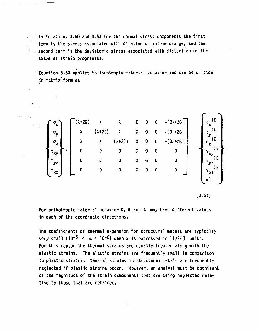
In Equations 3.60 and 3.63 for the normal stress components the firstterm is the stress associated with dilation or volume change, and the
second term is the deviatoric stress associated with distortion of the
shape as strain progresses.
Equation 3.63 applies to isentropic material behavior and can be writtenin matrix form as
: oax (X+2G) A 0 0 0 -(3X+2G) cx IE
ay A (X+2G) A 0 0 0 -(3).+2G) C IE
a X X (A+2G) 0 0 0 -(3A+2G) c IE
TXy . 0 0 0 G 0 0 ° JE
Xyz 0 0 0 0 G 0 0 y1E
Txz 0 0 0 0 0 G 0 1E
aT
(3.64)
For orthotropic material behavior E, G and may have different valuesin each of the coordinate directions.
The coefficients of thermal expansion for structural metals are typicallyvery small (10-5 c a 10-6) when a is expressed in [l/OF] units.
For this reason the thermal strains are usually treated along with the
elastic strains. The elastic strains are frequently small in comparison
to plastic strains. Thermal strains in structural metals are frequently
neglected if plastic strains occur. However, an analyst must be cognizant
of the magnitude of the strain components that are being neglected rela-
tive to those that are retained.
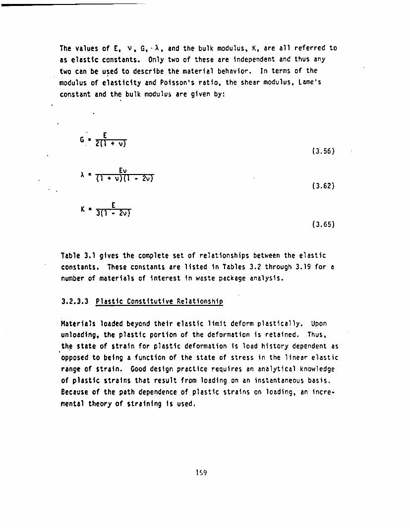
The values of E, v, G , and the bulk modulus, K, are all referred toas elastic constants. Only two of these are independent and thus any
two can be used to describe the material behavior. In terms of themodulus of elasticity and Poisson's ratio, the shear modulus, Lame's
constant and the bulk modulus are given by:
*G EG 2(1 * v)
(3.56)
Ev( + )(l - 2)
(3.62)
K s 3(]--E
(3.65)
Table 3.1 gives the complete set of relationships between the elasticconstants. These constants are listed in Tables 3.2 through 3.19 for anumber of materials of interest in waste package analysis.
3.2.3.3 Plastic Constitutive Relationship
Materials loaded beyond their elastic limit deform plastically. Uponunloading, the plastic portion of the deformation is retained. Thus,the state of strain for plastic deformation is load history dependent asopposed to being a function of the state of stress in the linear elasticrange of strain. Good design practice requires an analytical knowledgeof plastic strains that result from loading on an instantaneous basis.
Because of the path dependence of plastic strains on loading, an incre-
mental theory of straining is used.
159

Table 3.1
Relationships between Isotropic Elastic Constants
0%
LhM_ CONSTWTS VING'a "M. roisotI'n MATI BULK Mt.
A C( A (IFAR i*m.) E v .
.- _- . Gt31 1A 3A a2-
l o ( -IA ,6j 1 ~ A -- E A I C A 3 4 I 2 ( A~4,G _ __. A t G 1 {A+G} |
Revho-2v) A I Atv_(1-2v3 -_
A.R -- 3(K~~~- JK~-AJ J A
fJet f2C-M~ GE- -2J*C
C ,G V -_ 2GI1 __fv
OK JK-20 I r3K2.5!. t l6,^ __ __ C[t-2a'] *__ __
_ _ _ _ _ _ _ _ .
CV 114Wv (i-2v0 Y1rir . -- s-7vT
3JK-C, K 3K-
3XV 3 1 -2v) __

Table 3.2
Zircaloy-2 Tubing Mechanical Properties as a Functionof Temperature in English Units
T E(OF) (106 psi)
7510020030033740U500600700800900
10001100
13.813.713.212.717.512.211.711.210.710.29.79.?8.7
(-)
.32
.41
(106 psi)
C5.24
4.43
(106 psi)
9.06
20.41
K(106 psi)
12.6
23.2
4.624.624.624.624.624.6Z
.4.624.624.624.624.624.624.62
(10- 6 /OF)
Longitudinal Transverse
6.586.586.586.586.586.586.586.586.586.586.586.586.58
Radial
8.718.818.718.718.718.718.718.718.718.718.718.718.71
Legend
E - Elastic Modulus - Longitudinal Directionv - Poisson's RatioG - Shear Modulus (Lame's Constant )
- Lawe's ConstantK - Bulk Modulusa - Mean Coefficient of Thermal Expansion from 860F to Indicated Temperature
Coordinate definitionlongitudinal
- transverser - radial
Source: WE-65

Table 3.3
Zircaloy-2 Mechanical Properties as a Functionof Temperature in Metric Units
T(0C)
E(MPa)
V G(MPa)
A(MPa)
K(MPa)
.(1o- 6 /oc)
TransverseLongitudinal Radial
23.937.893.3148.9166.7204.4260.4315.6371.1426.7482.?537.8593.3
9.52x10⁴
9.45xl049. 10x104
8.76xl04
8.62xlO48.41x104
8.07x10⁴
7.72xlO4
7.38x10⁴
7.03x 10⁴
6.69x10⁴
6.34x1046.00x 104
0.32
0.41
3.61x10⁴ 6.25x10⁴ 8.69x10⁴
3.06xl4 14.08x10⁴ 16.14x10⁴
8.328.328.328.328.328.328.328.328.328.328.328.328.32
11.8411.8411.8411.8411.8411.8411.8411.8411.8411.8411.8411.8411.84
15.6815.6815.6815.6815.6815.6815.6815.6815.6815.6815.6815.6815.68
Leqend
E - Elastic Modulius-Lont itudinal Direction (Transverse Direction)v - Poisson's RatioG - Shear Modulus (Lame's Constant I)A - Lame's ConstantK - Bull Modulus
- Mea Coefficient of Thermal Expansion from 300C to the Indicated TemperatureCooruinate definition
z - longitudinal- transverse
r - radial
Source: Derived from data in Table 3.2

Table 3.4
Zircaloy- 'echanical Properties as a Functionof Temperature in English Units
T E v G 1 K(OF) (106 psi) (_) (106 psi) (106 psi) (106 psi) (10-6/OF)
Longitudinal- Radial
75 15.4 0.296 5.94 8.62 12.58 - -100 15.2 0.294 5.87 8.38 12.30 - -200 14.3 0.287 5.56 7.49 11.19 2.75 1.60300 13.5 0.280 5.27 6.71 10.23 3.00 2.22400 12.6 0.273 4.95 5.95 9.25 3.20 2.31500 11.8 0.266 4.66 5.30 8.40 3.33 2.82600 10.9 0.259 4.33 4.65 7.54 3.45 3.24700 10.0 0.252 3.99 4.06 6.72 3.52 3.52
G 800 9.2 0.245 3.69 3.55 6.01 3.60 3.72900 8.3 0.238 3.35 3.05 5.28 3.65 4.001000 7.5 0.231 3.05 2.62 4.65 3.70 4.221100 6.6 0.224 2.70 2.19 3.99 3.72 4.39
Legend
E - Elastic Modulusv- Poisson's RatioG - Shear Modulus (Lame's Constant v)A - Lame's ConstantK - Bulk Modulus
- Mean Coefficient of Thermal Expansion from 86°F t the Indicated TemperatureCoordinate definition
z - longitudinalr - radial
Source: WE-65
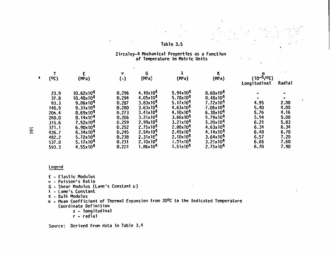
Table 3.5
Zircaloy-4 Mechanical Properties as a Functionof Temperature in Metric Units
G A(MPa) (MPa)
Ta (OC)
E(MPa)
V
()K
(MPa)a
(10- 6 /oC)Longitudinal Radial
23.937.893.3148.9204.4260.0315.6371.1426.7482.2537.8593.3
10.62x10⁴
10. 48x104
9.86x10⁴
9.31 x 1048.69x104
8.14x1C 4
7.52x10⁴
6.90x10⁴
6.34x10⁴
5.72x10⁴
5.17x10⁴
4.55x,14
0.2960.2940.2870.2800.2730.2660.2590.2520.2450.2380.2310.224
4. 10x104
4.05x10⁴
3.83x10⁴
3.63x1043.41x104
3.21x10⁴
2.99x10⁴
2.75x10⁴
2.54x1042.31xOo2.10x104
1.86x10⁴
5.94104
5. 78x1045.17x104
4.63x1044.lOX i04
3.66x1043. 21 x 1042.80x104
2.45xjO2.IOX I04I .31XI041. 51 x104
8.6x 1048.48x104
7.72xjO47.06x1046.38x 1045.79x104
5.20x1044.63x104
4.14x10⁴
3.64x10⁴
3.21 x 1042.75x104
4.955.405.765.946.216.346.486.576.666.70
2.884.004.165.085.836.346.707.207.607.90
Legend
E - Elastic Modulusv - Poisson's RatioG - Shear Modulus (Lame's Constant i)A - Lame's ConstantK - Bulk Moduluso - Mean Coefficient of Thermal Expansion from 300C to the Indicated Temperature
Coordinate Definitionz - longitudinalr - radial
Source: Derived from data in Table 3.4

Table 3.6 ;.~ ~~ ~ I . .
*Carbon Steel Mechanical Properties as a Functionof Temperature in English Units
T(OF)
E(106 psi) ( -) (106 psi) (106 A
1:(106 psi) (10k-/OF)
70100150200250300350400450500550600650700750800
27.9 .29 10.81 14.93 22.14
Ln
27.7
27.4
27.0
26.4
25.7
24.8
6.076.136.256.386.496.606.716.826.927.027.127.237.337.447.547.65
Legend
E - Elastic Modulusv - Poisson's RatioG - Shear Modulus (Lame's Constant j)K - Bulk Modulusa - Mean Coefficient of Thermal Expansion - Going from 700F to Indicated TemperatureA - Lame's Constant
Source: ASME-71

Table 3.7
Carbon Steel Mechanical Properties as a Functionof Temperature in Metric Units
T(OC)
E(MP a)
V G(MPa)
A(MPa)
K(MPa)
Ca(10o61oC)
21.137.865.693.3
121.1!48.9176.7204.4232.2260.0287.8315.6343.3371.1398.9426.7
19.2x 10⁴ 0.29 7.46x10⁴ 10.30x10⁴ 15.27x10⁴
l9.1 xl4
18.9x10⁴
18.6x 10⁴
18.2x10⁴
17.7xl4
17. 1x10⁴
;C.9311.0311.2511.4811.6811.8812.0812.2812.4612.6412.8213.0113.1913.3913.5713.77
Legend
E - Elastic Modulusv - Poisson's RatioG - Shear Modulus (Lame's Constant )A - Lames ConstantK - Bulk Modulusc - Mean Coefficient of Thermal Expansion - Going From 21.10C to the Indicated Temperature
Source: Derived from data in Table 3.6

Table 3.8
304- Stainless Steel Mechanical Properties asof Temperature in English Units
a Function
T(OF)
E(MPa)
":. 3
v
.29
6G(106 Ps') (106 psi)
I.(106 psi)
22.4670100150200250300350400450500550600650700750800
10.97 1!. 15
-
27.7
27.1
26.6
26.1
25.4
24.8
24.1
( 1- 6 /OF)
9.119.169.259.349.419.479.539.599.659.709.769.829.879.939.9910.05
Legend
E - Elastic Modulusv - Poisson's RatioG - Shear Modulus (Lame's Constant ii)A - Lame's ConstantK - Bulk Modulusa - Mean Coefficient of Thermal Expansion in Going From 700F to the Indicated Temperature
Source: ASME-71
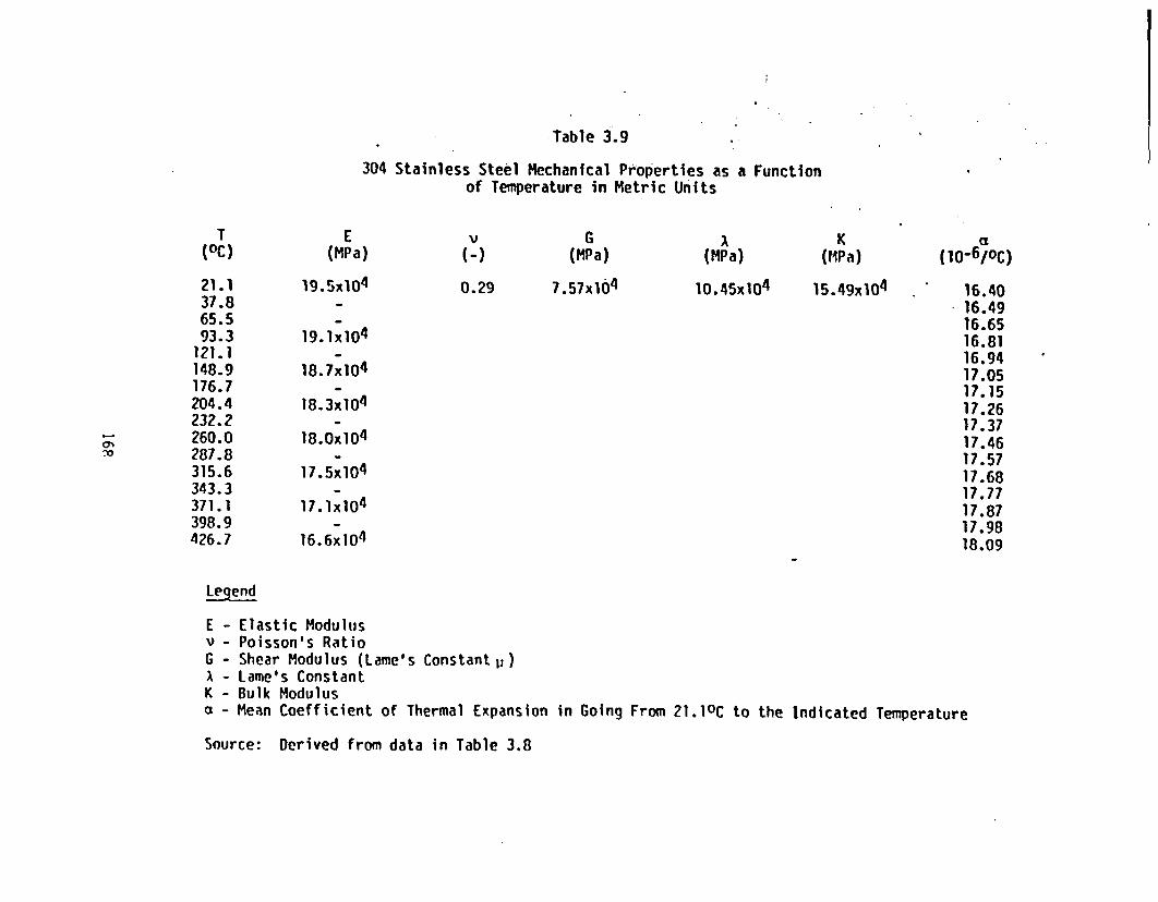
Table 3.9
304 Stainless Steel Mechanical Properties as a Functionof Temperature in Metric Units
T(DC)
E(MPa)
l9.SxlO4
V G(MPa)
7.57x10 4
(MPa)K
(MPa)
l5.49x104
a( 1-6/oC)
21.137.865.593.3121.1148.9176.7204.4232.2260.0287.8315.6343.3371.1398.9426.7
0.29 10. 45x104
19. X10 4
18.7x10⁴
18.3x10⁴
18. ox 1 04
17.5x10⁴
17. 1x 10⁴
16.6x10⁴
16.4016.4916.6516.8116.9417.0517.1517.2617.3717.4617.5717.6817.7717.8717.9818.09
a%
Legend
E - Elastic Modulusv - Poisson's RatioG - Shear Modulus (Lame's Constant,,)A - Lame's ConstantK - Bulk Modulusa - Mean Coefficient of Thermal Expansion in Going From 21.10C to the Indicated Temperature
Source: Derived from data in Table 3.8
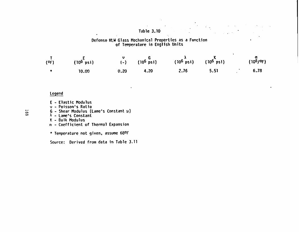
Table 3.10
Defense HLW Glass Mechanical Properties as a Functionof Temperature in English Units
T(OF)
E(106 psi)
V G(106 psi)
4.20
A(106 psi)
2.76
K(106 psi)
a(l1OG/OF)
10.00 0.20 5.51 6.78
Legend
ID
E - Elastic Modulusv - Poisson's RatioG - Shear Modulus (Lame's Constant )A - Lame's ConstantK - Bulk Modulusn - Coefficient of Thermal Expansion
* Temperature not given, assume 680F
Source: Derived from data in Table 3.11
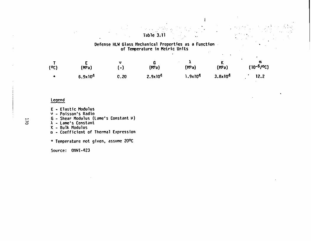
i
Table 3.11
Defense HLW Glass Mechanical Properties as a Functionof Temperature in Metric Units
. .q
. . .q . -
I
(10- 6 /oc)
12.2
T
(0C)
*
E(MPa)
6.gx104
V
C )
C. 20
G(MPa)
2.9x10⁴
(MPa)
1.9x10⁴
K(MPa)
3.8xI04
Legend
I-.-jC)
E - Elastic Modulusv - Poisson's RadioG - Shear Modulus (Lame's Constant ii)A - Lame's ConstantK - Bulk Modulusa - Coefficient of Thermal Expression
* Temperature not given, assume 200C
Source: ONWI-423

Table 3.1?
Commercial HLW Glass Mechanical Properties as a Functionof Temperature in English Units
T(OF)
E(106 psi)
10.0
v
(-)
0.20
(106 psi)
4.2
A(106 psi)
2.76
(106 psi)
5.51
a(!0- 6 /oF)
5.56*
Legend
E - Elastic Modulusv - Poisson's RatioG - Shear Modulus (Lame's Constant p)A - Lame's ConstantK - Bulk Modulusa - Coefficient of Thermal Expansion
* Temperature not given, assume 680F
Source: Derived from data in Table 3.13

Table 3.13
Comercial HW Glass Mechanical Properties as a Functionof Temperature in Metric Units
T(0C)
E(MPa)
6.9x10⁴
0-)
0.20
G(MPa)
2.9x 10⁴
A(MPa)
1 .9x104
K(MPa) (10- 6 /oC)
3.8x10⁴ 10.0
Legend
D.-
E - Elastic Modulusv - Poisson's RatioG - Shear Modulus (Lame's Constant )A- Lame's ConstantK - Bulk Modulusa - Coefficient of Thermal Expansion
* Temperature not given, assume 200C
Source: ON1-423

Table 3.14
Cast Iron Mechanical Properties* as a Functionof Temperature in English Units
T(OF)
E(106 psi)
23.6
v
(-)
0.271
(106 psi)
9.3
(1061psi)
9.4
K(106 psi)
17.23270
100200300400500600
(106 OF)'
6.5036.6266.7247.0487.3727.6978.0218.346
Legend
* Malleable IronE - Elastic Modulusv - Poisson's RatioG - Shear Modulus (Lame's Constant )A- Lame's ConstantK - Bulk Modulusa - Average Linear Coefficient of Thermal Expansion Over the Temperature Range from
320F to the Indicated Temperature
Source: BA-78
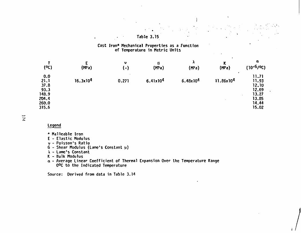
. - . t�
Table 3.15
Cast Iron* Mechanical Properties as a Functionof Temperature in Metric Units
T(0C)
0.021.137.893.3148.9204.4260.0315.6
E(MPa)
16.3x10⁴
(-)
0.271
G(MPa)
6.41x10⁴
A(MPa)
6.48x10⁴
K(MPa)
ll.86x104
a
(10- 6 /oC)
11.7111.9312.1012.6913.2713.8514.4415.02
-4
Legend
* Malleable IronE - Elastic Modulusv - Poisson's RatioG - Shear Modulus (Lame's Constant j)
X - Lame's ConstantK - Bulk Modulusa - Average Linear Coefficient of Thermal Expansion Over the Temperature Range
0OC to the Indicated Temperature
Source: Derived from data in Table 3.14
4/
Table 3.16
* Bentonite Mechanical Properties as a Functionof Temperature in English Units
T(OF)
E(106 psi)
v(-
G(106 psi)
p(106 psi)
K(106 psi)
C
(10- 6 /OF) -
-,
Table in Preparation
Legend
E - Elastic Modulusv - Poisson's RatioG - Shear Modulus (Lame's Constant P)A - Lame's ConstantK - Bulk Modulusa - Coefficient of Thermal Expansion
Table 3.17
Bentonite Mechanical Properties as a Functionof Temperature in Metric Units
T(OC)
E(MPa)
V G(MPa)
A(MPa)
K (MPa)
a(10-6/C)
-s
Table in Preparation
Legend
E - Elastic Modulusv - Poisson's RatioG - Shear Modulus (Lame's Cosntant ii)A - Lame's ConstantK - Bulk Modulusa - Coefficient of Thermal Expansion
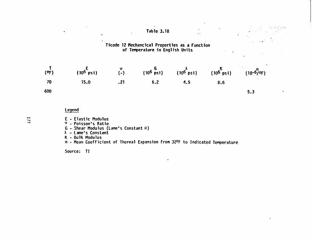
Table: 3. 18
Ticode 12 Mechancical Properties as a Functionof Temperature in English Units
T(OF)
70
E(106 psi)
15.0
v
(-)
.21
G(106 psi)
6.2
A(106 psi)
4.5
K(106 psi) 0l- 6aF)
[..6
600 5.3
Legend
-A
-I1E - Elastic Modulusv - Poisson's RatioG - Shear Modulus (Lame's Constant i)A - Lame's ConstantK - Bulk Modulusa - Mean Coefficient of Thermal Expansion from 320F to Indicated Temperature
Source: TI
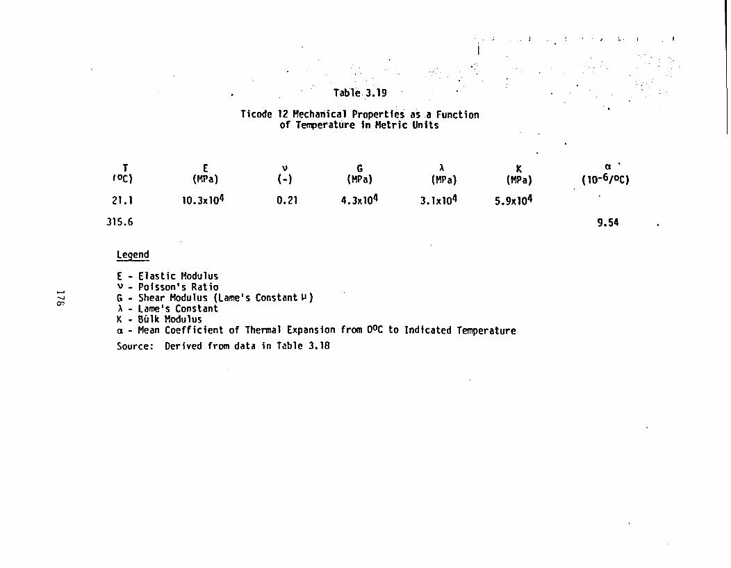
Table 3.19
Ticode 12 Mechanical Properties as a Functionof Temperature in Metric Units
. ., j L .
T2c)
21.1
E(MPa)
10. 3x10⁴
(-)
0.21
G(MPa)
4.3x10⁴
A(MPa)
3. 1x10⁴
K(MPa)
5.9x10⁴
CI
(10- 6 /oC)
315.6 9.54
Legend
-i0,
E - Elastic Modulusv - Poisson's RatioG - Shear Modulus (Lame's Constant I)
A - Lame's ConstantK - Bu1k Modulusa - Mean Coefficient of Thermal Expansion from OC to Indicated Temperature
Source: Derived from data in Table 3.18

Saint-Venant proposed in 1870 that the principal axes of the strain
components are coincident with the principal stress axes. In 1871, Levy
generalized (as did von Mises independently in 1913) the so-called
Saint-Venant-constitutive relationships to include both normal and shear
stress and strain components as follows:
.
(3.66)
which is also called a flow rule where:
CjJI total instantaneous strain component directedperpendicular to i and along j (elastic strainis ignored so jig 1 P)
CtrP a plastic strain component directed perpendicularto i and along j
Sij stress deviator tensor
dA - non-negative constant.
Equation 3.66 can be written on a component basis as
dcI dEI dcI dc I dc I dcISX'. W_~ . Sz r yz ZX C xy-. dA
x y z < d (3.67)
These equations, known as the Levy-Mises equations, are a constitutive
relationship between strain and stress on a component basis. They state
that the ratio of the increment of the total instantaneous strain component
(with elastic strain being neglected) to the corresponding stress deviator
component is a single constant for all components. The assumption that
the elastic strains are negligible in comparison to the instantaneous
plastic strains limits the theory to large strain conditions such as
would be encountered in metal-forming applications rather than structural
179
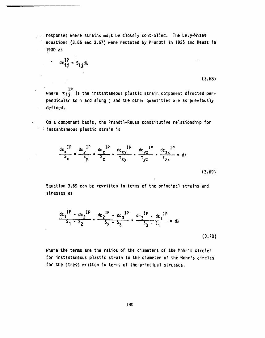
responses where strains must be closely controlled. The Levy-Mises
equations (3.66 and 3.67) were restated by Prandtl in 1925 and Reuss in
1930 as
IP
(3.68)
IPwhere Tij Is the instantaneous plastic strain component directed per-
pendicular to i and along j and the other quantities are as previously
defined.
On a component basis, the Prandtl-Reuss constitutive relationship for
* : instantaneous plastic strain is
de IP d IP
x ' y
dc IP de I de I P d I P
Z_ T Txy yz zx
(3.69)
Equation 3.69 can be rewritten in terms of the principal strains and
stresses as
dc1P - dc2 IP dc2IP-
SI S_ a ' T
- d 31 P
C S3
IP I dC3 . dcIa 3 -_ S K x d
(3.70)
where the terms are the ratios of the diameters of the Mohr's circles
for Instantaneous plastic strain to the diameter of the Mohr's circles
for the stress written in terms of the principal stresses.
180

The constant d can be shown to be equal to
3 d.ae
(3.71)31
The Prandtl-Reuss equations can be written for the instantaneous plastic
.strain components in terms of the stress components as:
I
dI P , dr x °~e
EI P , dE Iy a.e
[x
oy
- 1. (a + )
- I (a- 0]2 (° z
2 (x °y)z
dyIP
z dc rE z
= 3 dP7 ceTxy
dyP = 3dePdy Z -ETyze
dYIzP 3 T dc Tyzdyl P a 3 dE T2X
zx 7 Ge
(3.72)
121

: hr-. where
. '~I. .
Ce a' 2
(3.73a)
;' [(°l-a)2 + (a2 03)2 + (3a)2] 12
(3.73b)
:- a a' [(X°y)2 + (y ) 2 ( )2 + 6(T2 + T 2 + T2 1]e 77 z x XY yz z( )
(3. 73c)
Equations 3.73a through 3.73c express the von Mises yield criterion.
This criterion states that when any combination of stress components is
assembled as indicated on the right side of Equation 3.73a and its value
e is equal to the uniaxial yield stress in a tensile specimen, then
yielding will occur.
In 1924, Henckey developed a deformation theory for plastic stress-
strain behavior in which the strains are related to the current state of
stress. This theory is limited in its applicability because plastic
strains are typically dependent on the load path and better represented
by an incremental (local) relationship.
The Prandtl-Reuss constitutive relationship and von Mises yield cri-
terion as given in Equations 3.72 and 3.73 are frequently used to de-
scribe the instantaneous plastic stress-strain relationship.
182

3.2.3.4 Creep Constitutive Relationship
When tensile tests are performed, the stress-strain relationship depends,
in part, on the duration of the test. At elevated temperatures there is
more dependence on test duration. As the duration of the test is increased,
the load at fracture decreases. Also, if two specimens are tested so
that they are stressed in the range that includes some plastic instan-
taneous strain but not rupture, the specimen which is subsequently sub-
jected to the longer duration loading will retain more deformation on
unloading. This time effect of loading on deformation or strain is
called creep. The creep strain retained on unloading is conceptually
similar to the instantaneous plastic strain discussed in the previous
section.
The structural analyst must be concerned with creep because the associ-
ated strain consumes part of the ductility of the material. Figure 3.5
shows the creep strain versus time superimposed on the instantaneous
elastic and plastic strains. The instantaneous elastic strain will
always precede the creep strain. The instantaneous plastic strain may
or may not occur, depending on the proximity of the state of stress to
yielding as discussed in the previous section and in Appendix C (von
Mises yield criterion). The primary creep is a short duration process,
on the order of a day, in which the structure "shakes down" or flows to
a more stable condition to resist the imposed loading condition. Secondary
creep occurs within the time during which the rate of creep strain can
be approximated as a constant.
The creep rate which is the slope of the strain versus time curve of
Figure 3.5 is at a minimum in the secondary creep range. This is an
approximately constant strain rate region. The actual curve may be con-
cave downward over the initial time interval and concave upward over the
later time interval. In the tertiary creep range, the strain rate is
accelerating until rupture occurs. This is an unstable range, and the
stress levels should be kept low enough for the service temperature so
that the stable secondary creep range exceeds the service life of the
structure.
183

, I .
; . ... ..
qao
9rupture
4 ..
I
,~~~~~~~~~~~~~~
_
C
V6
tertiary creep
secondary
A
I. primary creep
I Itime
0
Figure 3.5
Plot Sowing nstataneous Elastic Strain A, nsiontaneous Plastic Strain BPlus Primary, Secondary and Tertiary Creep Ranges for Constont Stress
and Constant Temperature Controlled Uniaxiol Tensile Looding

-
A typical family of creep curves for a given temperature and stress
level is shown in Figure 3.6. Creep tests are performed for a limited
number of hours, and the service life of a structure may be greater than
the test duration. Assumptions are typically made and data extrapolated
to'longer loading durations. In general, structural system development
does not wait until creep test data are available for the entire loading
duration.
The family of creep curves shown in Figure 3.7 can be used in conjunction
with the instantaneous stress versus strain curve to give the stress
versus strain behavior for a given duration of the stress application.
These curves, known as isochronous stress-strain curves give a clear
indication of creep effects in terms of the additional strain incurred.
Waste package performance objectives will require keeping the stress low
enough so that the required service life can be endured without exceeding
a specified strain limit. There may be several strain limits, as higher
limits can be applied to bending than to membrane stress categories,
etc. For example, the ASME boiler and pressure vessel code specifies a
maximum membrane plus bending strain of 2 percent and a maximum membrane
strain of one percent away from welds.
Timoshenko has reviewed the creep rate data for various steels and has
observed that, initially, when the creep rate is decreasing (TI-56),
"the excess of creep rate above the minimum (whichapplies over the secondary creep range or at thepoint of inflection if concavity changes from downto up somewhere in the defined secondary creep range)decreases geometrically as time increases arithmetically."
The creep rate can be written as a function of time as
*c d *c a-btdt Cmin +ae
(3.74)
185
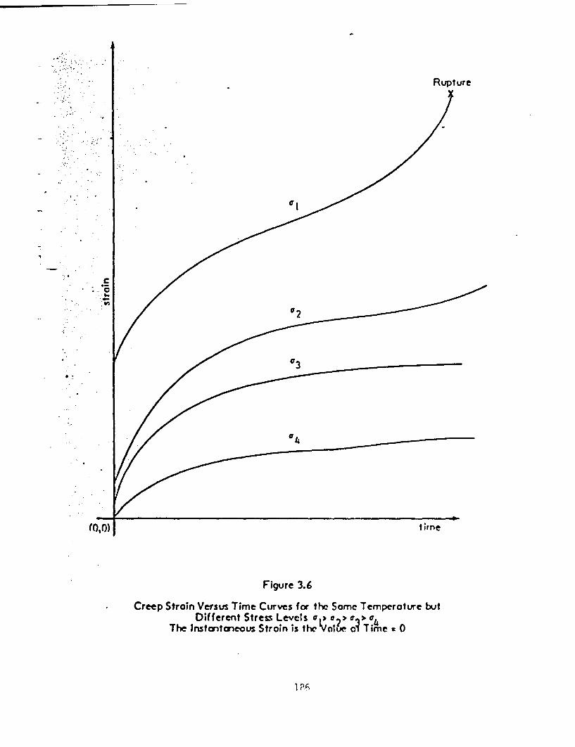
RI
IC
~~~~~~0 ~ ~ ~ ~ 0.
Figure 3.6
Creep Stroin Versus Time Curves for the Some Temperature butDifferent Stress Leves a a . a
The Instcntineovs Strain is the Yn'uot A ime 0
upt ure
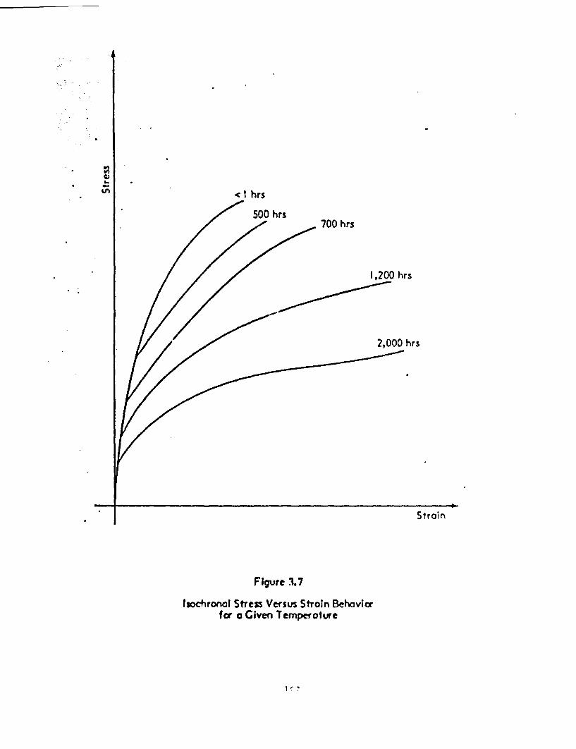
I-
hrs
500 hrs700 hrs
1,200 hrs
2,000 hrs
Strain
Figure 3.7
lsochronal StTess Versus Stroin Behaviorfor a Given Temperaftre
iCin which a, b and Cmin are constants that can be determined from creep
curves such as those shown in Figure 3.8.
Equation 3.74 can be integrated in time to give:
c c bC + mt a ebt
(3.75)'
where C and n are as shown in Figure 3.8. *c is the slope£ Cmin Emin iof the creep curve at the point of inflection. The dotted line is tan-
gent to the creep curve at the point of inflection.
Another plot is constructed from Figure 3.6 by taking the slopes of the
curves at given time intervals and plotting them on a logarithmic scale
against time as shown in Figure 3.9. This set of curves for different
values of stress can be used to determine values of the constants a and
b in the last term of Equation 3.75. The exponential is a correction
term which is added to the linear value given by the first two linear
terms on the right side of Equation 3.75. The exponential term is used
to approximate the distance parallel to the strain axis between the
straight dashed line and the curve of Figure 3.8 on the left side of the
inflection point of the curve. For large values of time, the term can
be neglected because it decays exponentially.
A study of experimental data by many investigators indicates that the
minimum creep rate can be represented empirically as a power function of
.the stress value
iC nCmin * ke
(3.76)
where, for a family of curves as shown in Figure 3.6, k and n are constants
for a given material and temperature.
1 o
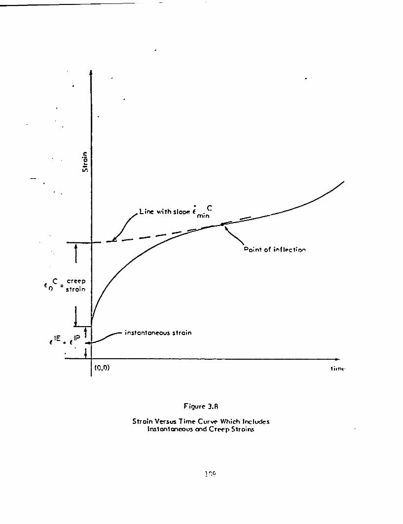
CI-)
Line with sloDe CZ/, -- mn
>/ _
Point of infKectom
f C creepn) strain
instantaneous strain(IE
(0,0)
Figure 3.8
SiTOin Versus Time Curve Which IncludesInstontoncous and Creep Sroir s
1 !^.G

al
03
04 for
0
0.b-
a
Is
2
U
CIc
for v4
I
I ifle
Figure 3.9
Creep Rote Versus Time Plotted From Fiqure 3.6 Doto
190
Creep data measurements require a long-term cormrnitment of laboratory
facilities and monitoring by technicians. The three principal parameters
governing the creep rate are stress state, duration of loading, and
temperature:.
c* f(C.t;T)
(3.77)
where
cc creep rate [t1 )
a = state of stress [f/2]
t duration of loading condition causingthe stress state (t]
T = temperature of material [e].
The developer of the correlation has some freedom in choosing the functional
form of the correlation. It is convenient if the independent parameters
are separated into three functions obeying the commutative law
- f ()f (t)f (T)a t T
(3.78)
This form is arbitrary and like other correlatings is not the true func-
tional relationship. Therefore its derivatives are not meaningful.
However, functions of the form of Equation 3.78 provide represenative
values of creep strain when properly developed. An appropriate set of
constants can often make a mediocre functional form yield acceptable
values within a limited range of the independent variables.
Difficulty is frequently encountered when data are needed for a particular
alloy and range of stress, temperature, and time (of loading). Furthermore,
most experimental data are obtained from uniaxial tensile loading.
I?1
M� I W
The most commonly used stress function is one given by Norton in 1929 as
fG(a) kom(3.79)
where k and m are experimentally correlated constants. Other correlation
forms have been proposed by McVetty in 1934, Soderberg in 1936, Johnson
.in 1963, and Garafalo in 1965 (Reference PE-71).
Time functions are like stress functions in that they represent approxi-
mately the dependence of the creep strain within a limited range of
variations of that quantity. The physics of creep can not be inferred
from these functions. A time function was developed by Andrade in 1910
ft(t) (l+btl/3) exp(kt)-l
(3.80)
where b and k are empirically determined constants. Other time functions
were developed by McVetty in 1934 and Graham and Wal les in 1955 (Reference
PE-71).
For material absolute temperatures below about 40% of the melting tem-
perature, creep occurs primarily by a slip mechanism at grain boundaries.
This slip creep straining is very similar to instantaneous plastic strain-
ing. The creep straining occurs over an interval of time but can occur
at much lower stress levels than the instantaneous plastic strain. Dorn
.in 1955 (Reference PE-71) suggested that the temperature function should
be of the form
f T) exp ( )
(3.81)
192

where
Q material's activation energy [e/molecule)
R Boltzmann's constant(a 1.38066 x 10⁻²³ Joules/molecule OK)
T material's absolute temperature [e]
It is also common for experimentalists to develop creep correlations
using a mixed stress and time function. Equation 3.77 is represented
as
cC f t(ct) f(T)at ~~~~~~~~~~~~~(3.82)
rather than by Equation 3.78. Marin gives various stress-time functions.
One given by Finnie in 1959 (Reference Ma-62) is
f t(oct) k k2 tk3
(3.83)
where
kl, k2, and k3 * empirical constants
a tensile stress [f/L2 I
t duration of stress condition rt]
Equations 3.77 through 3.83 are based on the creep correlation technique.
Because so many stress, time, stress-time, and temperature functions
have been developed, their detailed review is beyond the scope of this
report.
It should be remembered that the correlations are primarily for niaxial
tensile loading and that they are data representations rather than mathe-
matical expressions of the physics of creep. Usually, creep correlations
apply over the secondary range of creep where the creep rate is nearly
constant over a significant period of time. Also, deviations from the
constant creep rate can be corrected for limited loading durations by
the last term in Equation 3.75.
In 1950, Drucker unified the flow rule relationships for elastic and
inelastic deformation by defining the plastic potential function
p P(o.)
(3.84)
as a scalar function of the stress components Oij. He then expressed the
incremental creep shown in terms of the plastic potential function as:
dcij v- 2 dX
(3.85)
and where
dcc
/TBmn amn
(3.rE6)
where dce t equivalent creep strain increment.
Equation 3.85 can be written as
dcc BPdc
di ,0ij a(
(3.,q7)
194

The plastic potential function is written in terms of an equivalent
stress. The stress components are summed so that the equivalent stress
is comparable to the uniaxial stress in a tensile test. The von Misesequivalent stress is most often used although multicomponent creep data
verifying its applicability are very limited. The form of the von Mises
yield is given by Equations 3.73c for isotropic materials. Its derivative
is given-as
8:x _ e [y zF 1
(3.88)
If the potential function is assumed to have a form of
k2Ploij) k e
(3.89)
and it is further assumed that:
2 ' [(1-o2) + (2-o3)2 + (3-cl)2]
(3.90)
then the constants kl and k2 can be determined from Equations 3.89 and
3.90:
kl
k2 2 (3.91)
The effective creep strain s e can be defined as:
dc C 2 dC dcC
(3.92)
195
The constitutive relationship in incremental form becomes
dcC
dcoa _ e S
(3.93)
where Sij is the stress deviator tensor.
Differentiating Equation 3.78 with respect to time gives
dcc fo(°)t) fT(T).dt C dt T
(3.94)
This is known as the time hardening law for uniaxial creep.
The flow law can be written on a multi-axis basis as
dci C a~ e d ft(t) f(T)dt.ic a fo(°e) Gail dt
(3.95)
The flow rule or constitutive relationship applies to constant volume
creep straining processes where straining is a result of deviatoric
stresses, Sij, only and where the axes of principal stresses and strains
coincide.
By substituting the value of ae/aax from Equation 3.88, Equation 3.95
can be written for the various incremental strain components as:

dc fo°e)
Yxy ae T:
e
dcC 3 oe a
C 3fr(Ce)dcY 0 e3fr(0e)dy = r
3f (0e)e
] dft(t)- 7(Cy + o:Z ) dt
( df (t)- 2 ox + Cz) dt
] df (t)- -T (ox + y ) dt
fT(T) dt
fT(T)dt
fT(T)dt
dft(t)
xy dt
df t(t)
yz dt
fT(T) dt
fT(T)dt
dft(t)
zx dt
(3.96)
This constitutive relationship is the most important analytical element
of the mechanics of creep. The discussion of creep can be extended to
encompass the creep.strain's dependence on time and temperature so the
relative influence of these two parameters is appreciated. Response
197

curves are shown in Figure 3.10. These curves are generated by the
locus of constant strain points or failure points on a stress versus
time-temperature parameter (TTP) plane. The curves are useful for
sel'ecting a design stress based on an allowable creep strain for a given
load duration and material temperature. It should be noted that the data
given in Figure 3.10 are typically on the basis of uniaxial tensile
loading and uniaxial stress. For performance evaluation of an actual
structure, the state of stress may be bi-axial or tri-axial and hence
more complex. The upper curve shown in Figure 3.10 is known as a stress
rupture curve. It indicates what stresses cause failure for a given
load duration and temperature. The various curves can indicate what
limits on stress levels are needed to keep the creep strain and de-
formations within acceptable limits. The creep strain is related to the
total strain as
(3.97)
where
C total strain at a point [ ]
cI instantaneous strain at a point due toinstantaneous elastic, thermal, andinstantaneous plastic deformations r
Cc= creep strain at a point. [ )
The most commonly used TTP is the Larson-Miller parameter (LMP) published
by Larson and Miller in 1952.
TTP LMP T(kl + log t)
(3.98)
.1

4,
Rupture
\~~( \
TTP
Figure 3.10
Curves of Constant Creep Strain nd Ruptureon Stress Versus Time-Temperoture Parameter P)
199
where
T - absolute temperature (R)
kl a constant (usually 20.0)
t time (hr)
Other TTP's have been developed by Dorn, Manson and Haeford, Fisher and
Dorn, and other investigators (Reference PE-71).
The fifth line in Table 3.20 presents the LMP value for a temperature of
2000 C and a loading duration of 1,000 hours. As shown in the fourth
line, dropping the temperature by 100C allows the loading duration to
increase by a factor of 3.1 to 3,140 hours for the same value of the
LMP. In line seven, an increase of 500C to 2500C causes the loading
duration to drop to 6.32 hours. The LMP when evaluated for different
temperature values indicates a very strong variation in the allowable
loading duration. For a given allowable stress or a given allowable
total strain, small increases in temperature drastically reduce the
allowable duration of the stress associated with the load condition.
Alternately, reducing the temperature greatly lengthens the allowable
load duration.
3.3 Loads and Constraints
The finite element method uses nodes whose initial position and velocity
are specified. These nodes can be translated along three orthogonal axes
and rotated about each of the three axes. These six components allow for
the description of any general motion condition.
For a structure to perform its primary function of transmitting loads
without failing (generally without breaking or incurring excessive de-
formation), it must be constrained. The constraints have many forms de-
pending on the physical nature of the structural anchors and foundation.
200

Table 3.20
Different Temperature and Load DurationsConsistent with a Constant LMP
T T t LMP(OC) (OR) (hrs)
50 581.4 4.80 x 10¹³ 19585.2(5.5 x 10⁹ years)
100 671.4 1.47 x 10⁹ 19585.2(1.7 x 10⁵ years)
150 761.4 5.23 x 10⁵ .9585.2(6 years)
190 833.4 3.14 x 10³ 19585.2
200 851.4 1.00 x 10³ 19585.2
210 869.4 3.34 x 10² 19585.2
250 941.4 6.32 x 100 1!'585.2
300 1031.4 9.68 x 10⁻² 19585.2(5.8 minutes)
400 1211.4 1.46 x 10⁻⁴ 19585.2(0.53 seconds)
500 1391.4 1.19 x 10⁻⁶ 19585.2(4.3 x 10⁻³ seconds)
201
To use the finite element method, the structural analyst must interpret
the physics of the structure and must specify a representative assemblage
of elements that are connected at nodes. Then, any or all of the six
degrees of freedom of any node can be constrained throughout the response
simulation. By specifying the various degrees of freedom that are con-
strained (eliminated) for any of the nodes in the model, the analyst ef-
fectively constrains the structure. The constraints allow the loads
imposed on the structure to be reacted causing loads (forces and moments)
and associated stresses internal to the structure.
Analytical problems that are solved using continuous functional relation-
ships typically involve the use of constraints in the form of algebraic
equations. They specify a particular point on the structure that s pre-
vented from translating or rotating in a particular direction. For
differential equations expressing displacement, the constraints are the
differential equation's boundary conditions.
For the finite element method of analysis, the external loads may be
specified as:
* Forces and moments applied at specific nodes (thisis usually in terms of three force components andthree moment components for the coordinate systems)
* Pressures acting on a particular element face
* Gravitational body force acting on the massassociated with each of the elements
Some programs allow for the centrifugal body force associated with the
mass of any element which is rotating at a specified velocity. This is
used in conjunction with particular element types for modeling rotating
cylinders or annuli.
External forces may also be applied indirectly by specifying the displace-
ment or rotation from a previous equilibrium position of various nodes.
This is done in terms of the three displacement components and three
rotational components that specify the position of a node.
202

The finite element method of analysis
types of loading and superimposes the
conditions are represented with ease.
lytical solutions for complex loading
allows the treatment of various
responses. Very general loading
It is not practical to obtain ana-
conditions.
3.4 Equations of Motion
.Equations of motion describe the motion at discrete points or nodes. These'
equations relate element conditions and behavior to node motion. The mass
of each element is allocated to the various nodes of the element. The
equation of motion then relates the element properties to the node motion.
For a simple two degree
the equations of motion
of freedom (ui, u2) system as shown in Figure 3.11
are:
Fml
L
0 U1
m2 U2
(CI+C 2) -C2 u
-C2 C2, u2
+ ( lk 2) -k 2 u |
L k2j( u2
C
)IF(t)
F2(t)
(3.99)
where:
Mi mass at node i cm]
Cj damping of element i [ft/U]
ki r stiffness of element i [f/t]
ui - displacement of node i [t]
ui z velocity of node i [L/t)
2ui - acceleration of node i [i/t
Fj(t) transient forcing function applied to node i IfI]
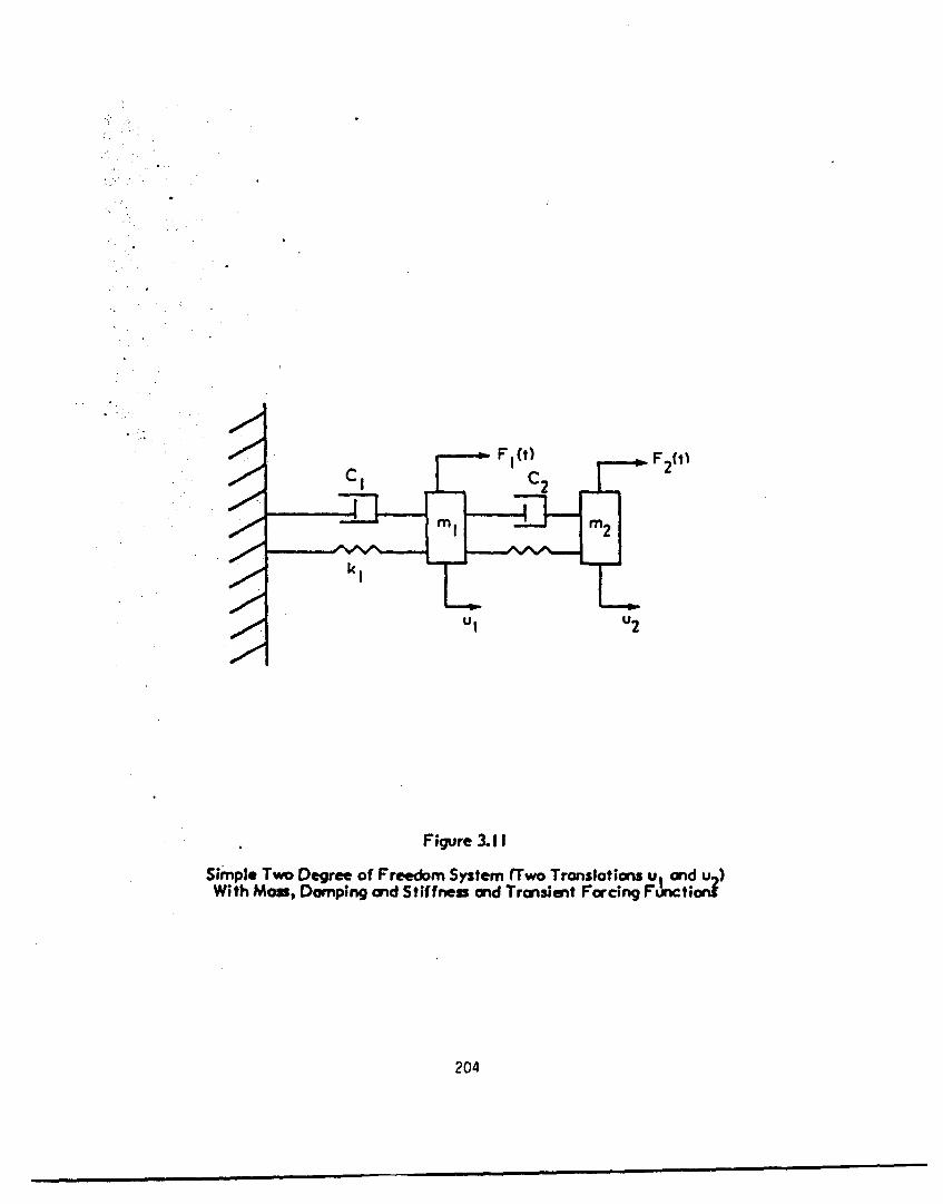
I:-:
Cl
Ul U2
Figure 3.11
Simple Two Degree of Freedom System Two Translations ul and u )With Mos, Damping and Stiffness and Transient Forcing Fuwcti
204
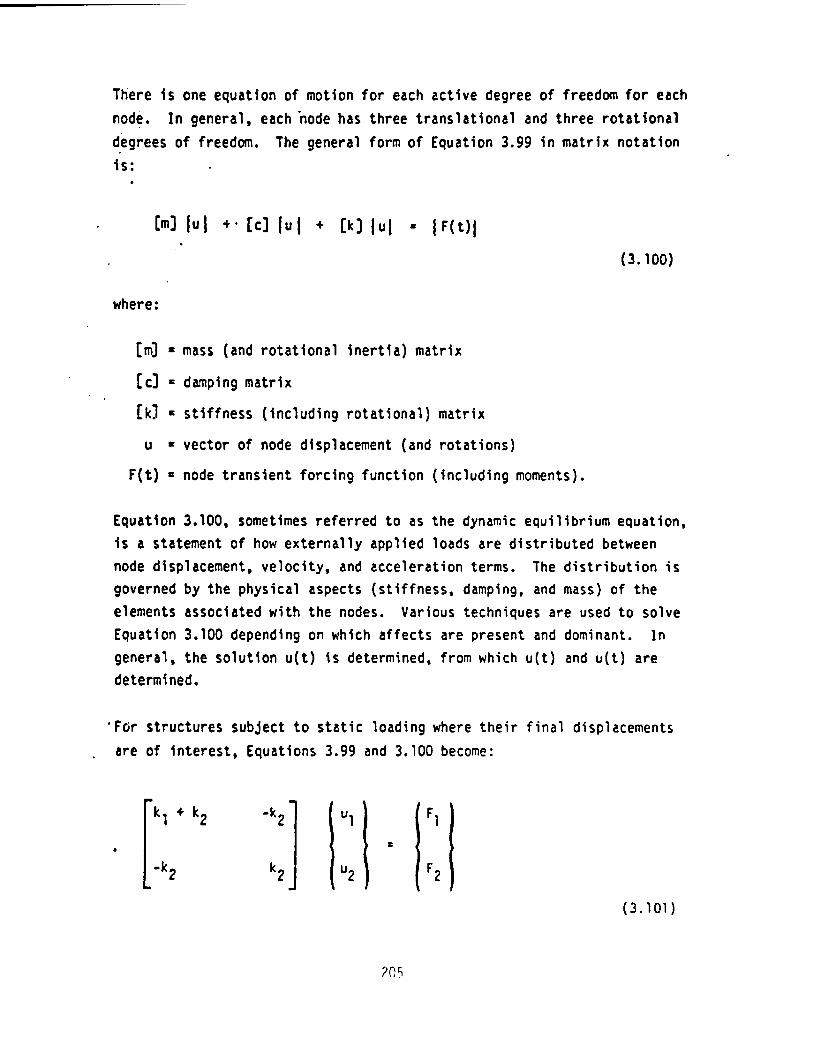
There is one equation of motion for each active degree of freedom for each
node. In general, each node has three translational and three rotational
degrees of freedom. The general form of Equation 3.99 in matrix notation
is:
Cm] ul + Ec] u + (k] u - IF(t)l
(3.100)
where:
[m) = mass (and rotational inertia) matrix
Ec] = damping matrix
Ck stiffness (including rotational) matrix
u a vector of node displacement (and rotations)
F(t) = node transient forcing function (including moments).
Equation 3.100, sometimes referred to as the dynamic equilibrium equation,
is a statement of how externally applied loads are distributed between
node displacement, velocity, and acceleration terms. The distribution is
governed by the physical aspects (stiffness, damping, and mass) of the
elements associated with the nodes. Various techniques are used to solve
Equation 3.100 depending on which affects are present and dominant. In
general, the solution u(t) is determined, from which u(t) and u(t) are
determined.
'For structures subject to static loading where their final displacements
are of interest, Equations 3.99 and 3.100 become:
kl + k2 A2 U(101
(3.101)
kiul .
(3.102)
where the quantities are as previously defined except that the force vec-
tor components do not vary with time. This is the relationship between
externally applied loading, element stiffness, and node displacement.
3.5 Equilibrium Relationships
Structural performance is always in accord with the principle of force and
moment equilibrium. Structures that are subjected to static loading and
that have no sustained motion obey the equilibrium principle at all loca-
tions throughout the structure. The static equilibrium condition is ex-
pressed in terms of each of the six degrees of freedom of motion:
UFr 0 F 0 a °' Fz a
r a ° SMe 0, Mz O
(3.103)
where:
a
Fj * force exerted on a nodeapplied force componenttype forces) [fJ
i the direction (externally.Id internal element stiffness
Hj * moment exerted on a node about a line parallel tothe I axis (externally applied moment componentand nternal element rotational stiffness typemoments) (fLJ
206
Some structures experience accelerations associated with transient or
periodic motion during their responses to loading conditions. These
structures conform to a special form of the equilibrium principle which,
for a particle, includes pseudo force (and moment) components directedopposite to the acceleration and having a magnitude equal to the productof the translational (rotational) acceleration and the mass (mass momentof inertia) of the particle. The finite element method includes procedures
for associating distributed mass from various elements with the accelera-
tion at discrete points (nodes). The node is usually the point of connection
of the elements contributing mass to the node. The pseudo force and moment
components are named in honor of D'Alembert who stated the principle of
dynamic equilibrium in 1743. The dynamic equilibrium relationships are:
Ur mr 0, F -ma0 0, F - ma aO
EM I E Os EM I~ Oz a
r Irar °. rM-1 0 6e 0,EMz - .0
(3.104)
wheie:
F* - force exerted on a node in the direction (externallyapplied force component and internal element stiffnessand damping type forces) If)
Mi moment exerted on a node about a line parallel to thei axis (externally applied moment component and internalelement rotational stiffness and damping type forces) [tf]
m mass associated with particle or node at which dynamicequilibrium condition is being applied [ml
1 * mass moment of inertia of the mass of a node about axis [mt2
al translational acceleration of the mass in the direction [E/t2)
al angular acceleration of the mass about the axis (l/t2J
207
This dynamic equilibrium principle states that a particle can be consid-
ered to be in force equilibrium if the inertial force of the mass corres-
ponding to its current acceleration magnitude is included along with the
external forces in the summation of forces on the particle.
This form of the equilibrium principle given by DAlembert is consistent
with Newton's second and third laws (about 1664) and of profound conse-
quence to the development of analytical mechanics and in particular to
Hamilton's principle.
The equilibrium condition is important because it is used to verify the
finite element solution. The finite element solution involves equations
of motion, load condition, and constraints, which are used to solve forthe structure displacement, which generally includes six degrees of free-
dom at each node, and the internal forces and moments at each node of each
element. The load path and displacements are established in accord with
the stiffness, damping, and mass distributions of the structure and the
nature and location of the constraints. The equilibrium relationship
requires the force and mment interactions among the elements to be in
force and moment equilibrium at each node with respect to each axis.
The equilibrium condition described in this section can be used as a check
on the solution accuracy. It must be satisfied to within a specified
tolerance. The force balance is similar to that given in the equation of
motion but differs in that it deals with internal forces, which have been
determined based on deflection, velocity, and acceleration calculated by
solving the equations of motion, which contain only external force terms.
The equations of motion are coupled and more difficult to solve than the
uncoupled equilibrium relationships.
Equilibrium checks are also useful when done for the entire structure.
They should indicate that the sum of the reactions in any of the six degrees
of freedom is of equal magnitude to the externally applied load (including
body forces such as gravity). The sum of all reactions (at the constraints)
should be of opposite direction to the externally applied loads.
3.6 Analytical Responses
The purpose of structural analysis is to simulate mathematically a con-strained structure's response to a particular loading condition. The
response quantities of a finite element analysis generally include:
Node positions (after loading)
Element deformation (between nodes based on positionbefore and after loading)
* Element strain (at each node of the element basedon deformation and previous dimensions)
* . Internal force and moment interaction for eachelement at each node
Linear-elastic force versus displacement material behavior is most commonwhere a constant value of element stiffness is used. Optional responsequantities usually include the stress tensor components at each node of
each element.
When the structure and its model are especially complex, static loads may
be imposed in steps so that the finite element model will go through theentire calculational procedure a number of times. This affords the program
the opportunity to perform node equilibrium checks and provides the analystwith incremental response versus incremental loading information. For
structures that respond dynamically, solutions are obtained at discrete
time increments. The values of the externally applied loads can be changed
at the end of each time step. This solution technique allows for the responsesto be determined incrementally over time. In this process, equilibrium
checks are optional after each time step. Equilibrium is attained to withina particular tolerance value when it is imposed. To speed up the calculation,
the analyst can specify a multiple of calculational time increments per
equilibrium check. When equilibrium checks are made, they are made for all
unconstrained degrees of freedom of all nodes.
209

Strains associated with changes of temperature of the structure are calcu-
lated as though the structure was free to expand without constraints (free
thermal expansion). The displacements are then considered in conjunction
with the constraints on the structure, the structural stiffness distribu-
tion, and node force and moment equilibrium. The constraints and element
stiffness give rise to internal forces and moments for which stresses can
be calculated on a linear elastic basis.
The analyst must also be concerned with instantaneous plastic or creep
strains. This involves specification of the parameters appearing in the
pertinent constitutive relationship. These are used in place of the gener-
alized Hooke's Law applicable to linear elastic behavior. The solution
procedure is very similar except that it is necessary to calculate the
stress tensor so that the instantaneous plastic flow rule can be evaluated
in terms of the current state of stress. The creep flow rule is evaluated
in terms of the current state of stress and the current duration of loading.
Responses of greatest interest to the waste package performance analyst are
those indicating pending undesirable performance. This undesirable perform-
ance is likely to take the form of excessive strain either for regions of
the structure that experience instantaneous plastic strain or for regions
where creep strains accumulate over long durations of loading. In the ab-
sence of these two phenomena, elastic strain limits would be imposed by the
familiar technique of limiting the stress tensor. This is accomplished by
limiting the stress in accordance with one of the yielding criteria. Several
yielding criteria are described in Appendix C.
210
s *~~~~~~~~- .- - .1 1. --
4.0 REFERENCES
ASME-71 1971 ASME Boiler and Pressure Vessel Code Section 111Nuclear Power Plant Components, ASME, 1971.
BA-78 Theordore Baumeister, et al., Marks Standard Handbook forMechanical Engineers, McGraw Hill, 1978.
CO-66 W.A. Coffman, et al., A Large Range Thermodynamic and TransportWater Properties FORTRAN IV Computer Program. WAPD-TM-568,December 1966.
CU-83 R.H. Curtis, R.J. Wart, and E.L. Skiba, Parameters andVariables Appearing in Respository Design Models, NUREG/CR-3586, December 1983.
FI-50 M. Fishenden and O.A. Saunders, An Introduction to HeatTransfer, p. 97, Oxford University Press, London, 1950.
GI-61 Warren H. Geidt, Principles of Engineering Heat Transfer,Van Nostrand, 1961.
HO-81 Jack P. Holman, Heat Transfer, McGraw Hill, 1981.
KR-61 Frank Krieth, Principles of Heat Transfer, InternationalTextbook Co., Scranton, Pennsylvania, 1961.
MA-62 Joseph Marn, Mechanical Behavior of Engineering Materials,Prentice-Hall, 1962.
MI-83 M. Mills, D. Vogt, and B. Mann, Parameters and VariablesAppearing in Radiological Assessment Codes, NUREG/CR-3160,June 1983.
ONWI-423 Engineered Waste Package.System Design Specification,Westinghouse Electric Corporation, OWI-423, May 1983.
ONWI-449 Dale R. Simpson, Some Characteristics of Potential BackfillMaterials, ONWI-449, May 1983.
ORNL-77 Oak Ridge National Laboratory, Documentation for the CCC-217/ORIGEN Computer Code Package, June 1977.
PE-71 R.K. Penny and D.L. Marriott, Design for Creep, McGraw-Hill,1971.
TI TIMET-TiCode-12, Titanium Metals Corporation, Pittsburg,Pennsylvania.
TI-56 S. Timoshenko, Strength of Materials, Part 11, AdvancedTheory and Problems, Third Edition, 1956, Van Nostrand.
WE-65 D.B. Scott, Physical and Mechanical Properties of Zircalloy2 and 4, Westinghouse Electric Corporation, WCAP-3269-41,May 1965.
WE-73 Reference Safety Analysis Report, RESAR-3, WestinghouseElectric Corporation, Vol. II, 1973.
212

APPENDIX A
RELATIONSHIP BETWEEN TEMPERATURE DEPENDENCEOF MASS DENSITY AND TEMPERATUREDEPENDENCE OF THERMAL EXPANSION
The mass density varies slightly with temperature for most structural
metals. Therefore, experimenters tend not to focus attention on its
temperature dependence. Frequently, only the room temperature value is
given in property tables. However, the thermal expansion coefficient of
temperature is frequently given as a function of temperature. This
appendix indicates how the thermal expansion coefficient data can be
used to quantify the dependence of mass density on temperature.
Assume that an isotropic cube with a side dimension L at the initial
uniform temperature T is raised in temperature to T2. Geometrically
each side will increase in length by an amount AL when the cube reaches
temperature equilibrium at T2. The increase in length
AL 3cLAT
(A-])
where
L increase in length of one side of cube [LI
a mean value of thermal expansion coefficient oftemperature in the temperature range fromT, to T2 ['/'e]
L i initial length of cube side El]
AT = T2 T1 - increase in temperature of the cube [el
During transition from the lower temperature T to the higher tempera-
ture T2,the mass of the cube remains constant
ml m 2
tlvl ' 2 V2(A- 2)
A 1
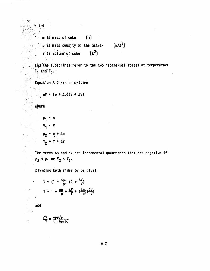
:...''where!
:I ; s mass of cube [n
p s mass density of thE
:: Y Is volume of cube
andthe subscripts refer toT1 and-T2-
Equation A-2 can be written
* pY ' (P + &P)( + V)
where
P1 P
P2 P+.P
V2, Y + V
The terms Ap and AV are nc
P2 < P1 or V2 < V1.
Dividing both sides by pV g
* 1 tl + AP) ( + V
1 I + A + A + (x(!LWV
n]
e matrix cm/d3J3
the two isothermal states at temperature
remental quantities that are negative if
ives
V
and
,AV i -P/P.VT 1 144/P
A 2

or
AV- ~~~~~~~~~~~~~~~~(A-3)
when higher order terms are assumed to be negligible (i.e., Ap/p<<l).
The change in volume can also be related to the change in the sidedimension
- 1V (L + -)3 O
which can be written as
AV 3L2 + 3L+ +
and
EY 3iC_ 33E2 _tL3L2 ~a3AV '--E + 2 +3
Substituting Eouation A-3 n the previous relationship yields
uc 32 a3
P - -. 2 - 3
(A-4)
as the density variation term. Substituting Equation A-1 for AL gives
3 3AT + 3(&6T)2 + (AT) 3
(A-5)
A 3
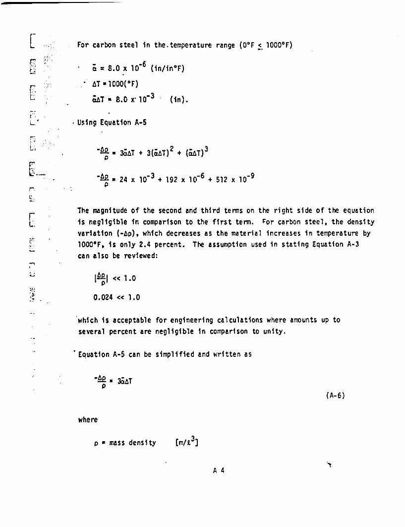
I . .I,.....
r" .. . I
I . .L: I
For carbon steel in the.temperature range (0°F < 1000°F)
= 8.0 x 10⁶ (in/in°F)
- 6T =1000(OF)
;LT 8.0 x 0 3 (in).
Using Equation A-5
-AO * 3AT 3(&AT)2 + (&AT)3Pr'
-AP 24 x 10-3 + 192 x 10 6 +P 512 x 0-9-
FL.
The magnitude of the second and third terms on the right side of the equation
is negligible in comparison to the first term. For carbon steel, the density
variation (-Lp), which decreases as the material increases in temperature by
1000F, is only 2.4 percent. The assumption used n stating Equation A-3
can also be reviewed:
I21 " 1.0
0.024 << 1.0.tIs
which is acceptable for engineering calculations where amounts up to
several percent are negligible in comparison to unity.
Equation A-5 can be simplified and written as
-A * 3ATp
(A-6)
where
p * mass density (m/t0
"IA 4
w s mean value of tbermal expansion coefficient oftemperature over the temperature range fromTt to T2 [t/te]
ET T2 --T temperature increase between isothermalstates and 2 (6]
AC)* r2 -Pa mass density increase of a given mass fora specific temperature increase(sT from T to T2) (m/g]3
-P -p2 * mass density decrease of a given massfor specific temerature ncrease(AT from T to T2) [m/ JI
Equation A-6 can be used to give an approximate but acceptable defini-tion of the mass density's temperature dependence in terms of availablethermal expansion coefficient data over a common temperature range.
In this report, we choose not to ignore the temperature dependence of
the mass density and approximate it by using Equation A-6 when thetemperature coefficient of thermal expansion data is available. Analysts
who use these data will be free to decide whether to treat mass densityas a temperature-dependent property or as a constant property for thetemperature variations anticipated in their particular application.This report presents consistent data to facilitate general analysis
requirements.
When finite element structural analysis methods are used, the analystmust consider the effects of using temperature-dependent mass density.
If .a given method assumes that no significant volume change occurs with
temperature changes, constant (non-temperature-dependent) values of
density should be used. In this instance, the mass of the structure is
calculated as the product of the mass density and the volume. To con-serve mass, a constant mass density (evaluated at the mean value of
temperature) should be used.
APPENDIX B
MOHR'S DIAGRAMS
Mohr's diagrams are graphic techniques for determining principal stresses,
maximum shear stress, principal strains, and maximum shear strains. These
graphic methods greatly aid the visualization of these quantities and their
variation between planes passing through the point of interest. Mohr's
*diagrams for stress and strain are only applicable to plane stress or plane
strains. For three-dimensional strain or stress Equations 3.5 and 3.34
must be solved to determine the principal strains and principal stresses.
The Mohr's diagram for stress is a graphic means of determining and dis-
playing the principal stresses and the maximum shear stress corresponding
to the state of stress at a point. The angles at which these principal
stresses are oriented are determined. In order to construct the Mohr's
diagram for stress, a state of stress must be defined. Because the
staff of stress varies with position within a structure, its definition
applies only to a particular position or point.
The state of stress is best defined with the aid of a diagram as shown
in Figure -l. The point in the structure at which the state of stress
i- being examined is denoted by an infinitesimal cube with one normal
and two shear stress components acting on each face.
The Mohr's diagram plotting procedure for stress involves examining each
of the planes individually, i.e., the xy plane, the yz plane, and the zx
plane. One circle, known as a Mohr's circle, is drawn for each plane.
-The sign convention for constructing a Mohr's circle for stress is shown
in Figure -2. Normal stress components are positive if they are tensile
(tending to stretch the material), and shear stress components are positive
if they act counter-clockwise. Figure B-3 shows an xy plane view of an
infinitesimal cube such as the one shown in Figure B-1. If the magnitudes
of these components are
ox * 20,000 psiay * 5,000 psiTxy a yx 5,000 psi
13I
.. mvv� ., .-
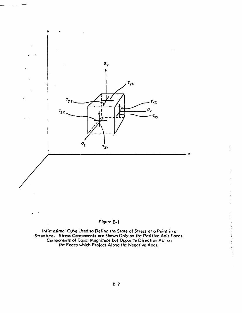
y
Tyx
7zx
xy
. X
Figure B-1
Infintesimol Cuke Used to Define the Stote of Stress of a Point in Structure. Stress Componens re Shown Only on the Positive Axis Foces.
Components of Equal Mognitude but Opposite Direction Act onthe Foces which Project Along the Negative Axes.
B 2
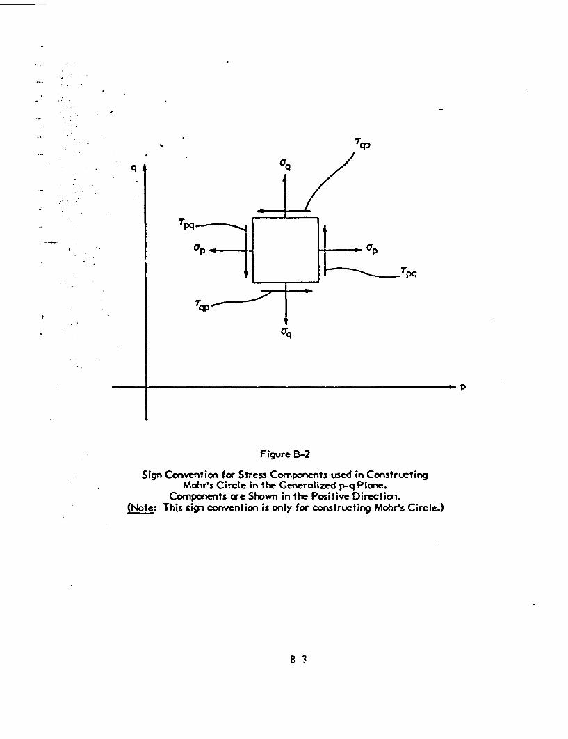
- .
- :
is
-- :e 1�17Tp
q aq
T pq
qap
ap
.r pq
- I p
Figure B-2
Sign Convention for Stress Components used in ConstructingMohr's Circle in the Generalized p-q Plane.
Components are Shown in the Positive Direction.(Note: This sign convention is only for constructing Mohr's Circle.)
B
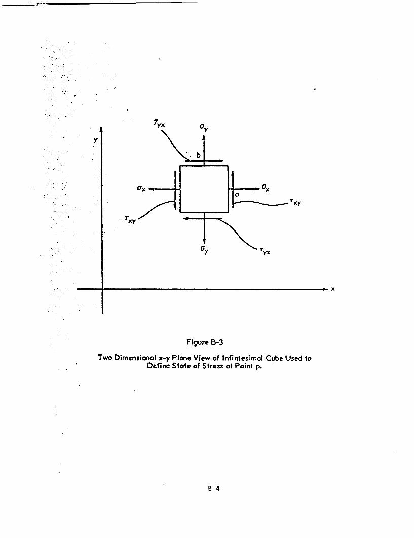
yx a
.~~~~
b
?xy
7.
XV~~~~~~~~~~~~~~~~~
#: -el: Onyx By~~(l 7y
Figure B-3
Two Dimenso x-y Plae View of Infintesmot Cube Used toDefine Stote of Stress at Point p.
4
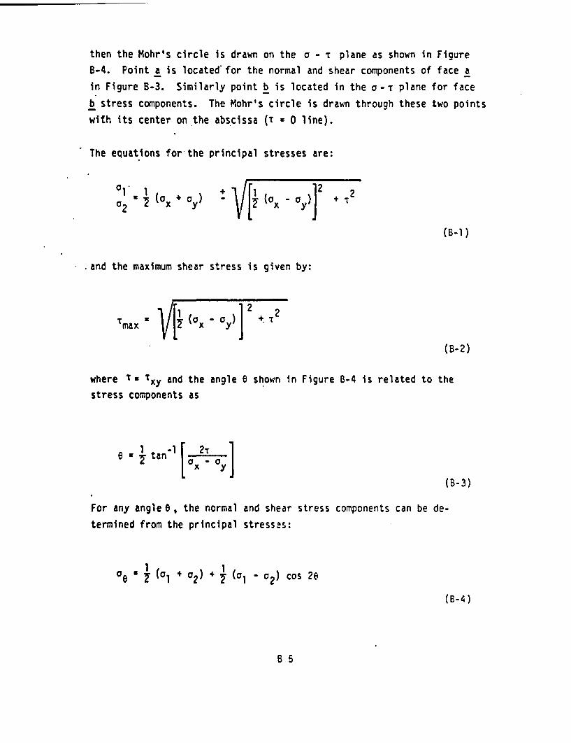
then the Mohr's circle is drawn on the a - T plane as shown in Figure
B-4. Point a is located for the normal and shear components of face a
in Figure B-3. Similarly point b is located in the a-T plane for face
b stress components. The Mohr's circle is drawn through these two points
with its center on the abscissa T = 0 line).
The equations for the principal stresses are:
a 2 x y (OX - y) + T2
(B-i)
.and the maximum shear stress is given by:
Tmax a T (aX - y) + 2
(B-2)
where X- xy and the
stress components as
angle e shown in Figure B-4 is related to the
6 a I tan 1 [2I cy2]
(B-3)
For any angle 6, the normal and shear stress components can be de-
termined from the principal stresses:
ae 7 ( + 2) + T (1 - 02) cos 26
(B-4)
B 5
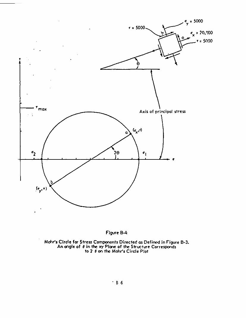
o 5000y
=
?Or)00_.= 5000
T
maxAxis of stress
a
y
Figure B-4
Mohr's Circle for Stress Components Directed as Defined in Figure B-3.An angle of e in the xy Plone of the Structure Corresponds
to 2 e on the Mohr's Circle Plot
- 6
Te (° a2) sin 2e
(B-5)
The three Mohr's circles for the stress in each of the planes can be
drawn on the same 0 - plane. One circle will circumscribe the othertwo smaller circles and each circle has one point in common with each of
the other two. These points in common lie in the a axis. Three Mohr'scircles for a hypothetical state of stress are shown in Figure -5. The
principal stresses are usually designated such that 01 > a2 > 3.
It is helpful when applying the Tresca criterion (see Appendix C) to
construct a diagram of the state of stress such as Figure -5. Thisfigure shows that the larger the Mohr's circle for stress, the greaterthe maximum shear (radius of largest circle). Also, the largest Mohr'scircle gives the largest difference in principal stresses (al - 2 inFigure B-5, which is equal to the diameter of the largest circle inFigure B-5). The Tresca criterion indicates failure will occur when thediameter of the largest circle equals that for failure of a simple uni-axial tensile specimen. A simple tensile specimen and its Mohr's circleare shown in Figure B-6.
Mohr's diagram for stress provides an opportunity to look at contrasting
cases of biaxial stress. Suppose that normal stress in the y directionshown in Figure B-3 was compressive, tending to compact the material,instead of tensile with the other components remaining unchanged. Thus
x 20,000 psiay -5,000 psiTxy ' tyX 5,000 psi.
(B-6)
The Mohr's circle shown in Figure B-7 is of much larger diameter thanthat of Figure -4. The yielding criteria as given by Tresca would
7
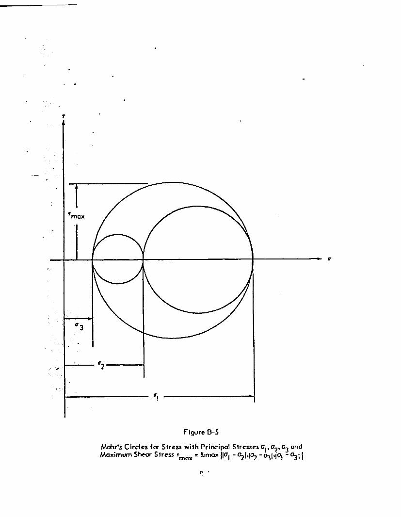
ac
T2
Figure B-S
Mohr's Circles for Stress with Principal Stresses Q 107 3 andMaximum Shear Stress 7max Lmax 1la7 - 02 1,12 -s'lom - °3 I
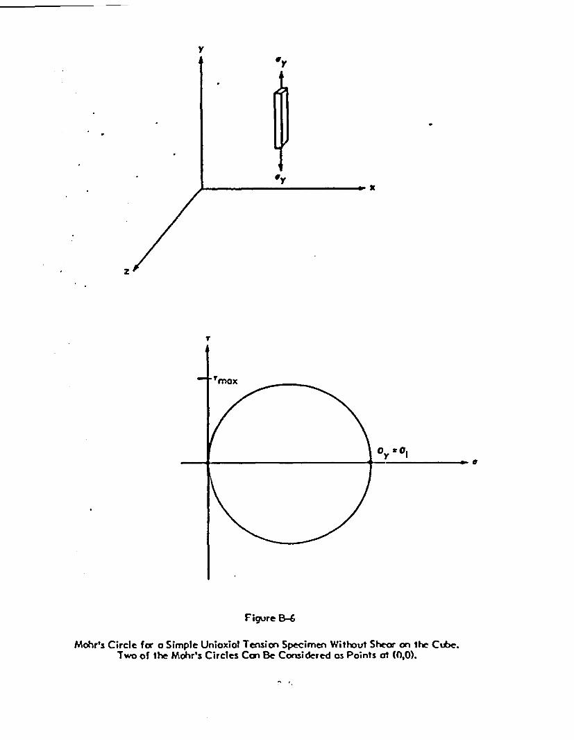
y
vT
UTY
2~~~~~~~~~~~~~
7max~~~~~~
Figure B4
Mohr's Circle for o Simple Unioxial Tnsi Specimen Witout Shear on the Ctbe.Two of the Mohr's Circles Can Be Considered as Points c (,0).
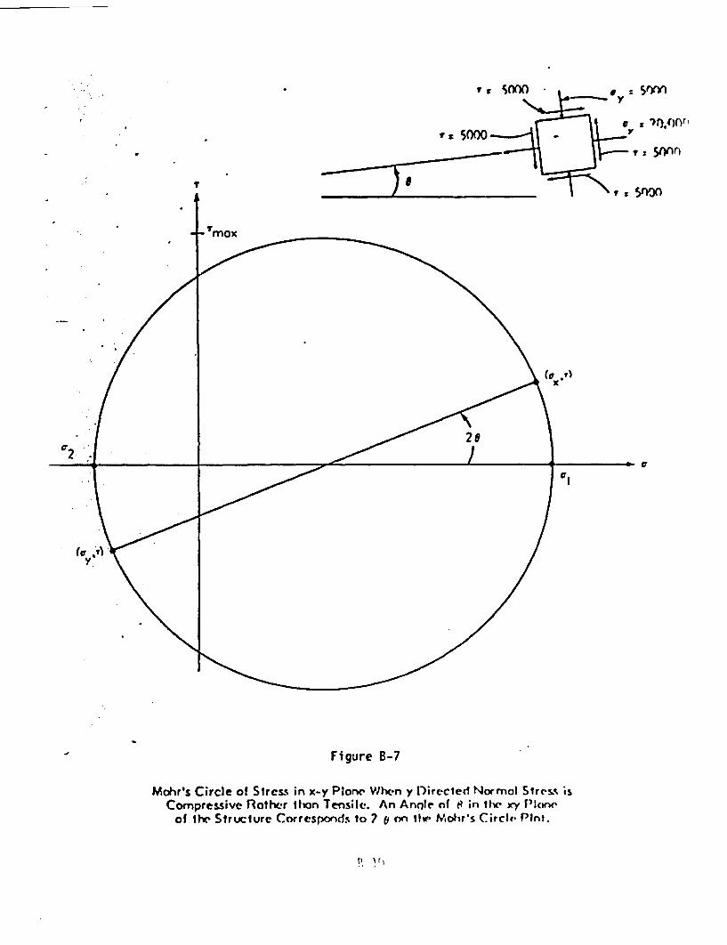
-
ItVW - -0y .
* z 5non
,
r
rmox
x
aaI
(a ,)y.
Figure B-7
Mohr's Circle of Stress in x-y Plane When y Directed Normol Stress isCompressive Ralher lon Tensile. An Annle of t? in the xy Ploni'
of the Structure Corresponds to 7 on the Mohr's Circle Plot.
p lrI
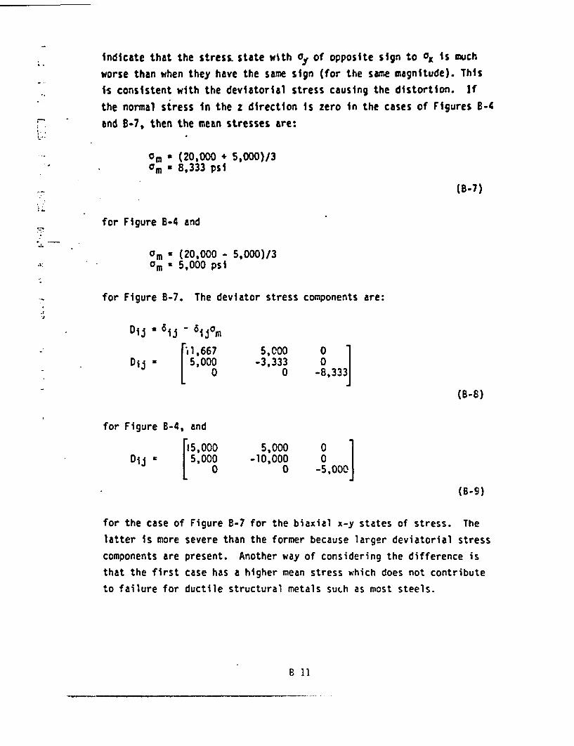
indicate that the stress state with ay of opposite sign to ° is much
worse than when they have the same sign (for the same magnitude). This
is consistent with the deviatorial stress causing the distortion. If
the normal stress in the z direction s zero in the cases of Figures -4
and -7, then the mean stresses are:15:
am - (20,000 5,000)/3a 8,333 psi
(B-7)
for Figure -4 and
am (20,000 - 5,000)/3am 5,000 psi
for Figure B-7. The deviator stress components are:
*.
Dij z 6 i 6ijoM
1.667 5,000 0Dij = 5,000 -3,333 0
0 0 -8,333
(B-B)
for Figure B-4, and
[5,000 5,000 0Dij 5,000 -10,000 0
- 0 -5000
(8-9)
for the case of Figure 8-7 for the biaxial x-y states of stress. The
latter s more severe than the former because larger deviatorial stress
components are present. Another way of considering the difference is
that the first case has a higher mean stress which does not contribute
to failure for ductile structural metals such as most steels.
B 11
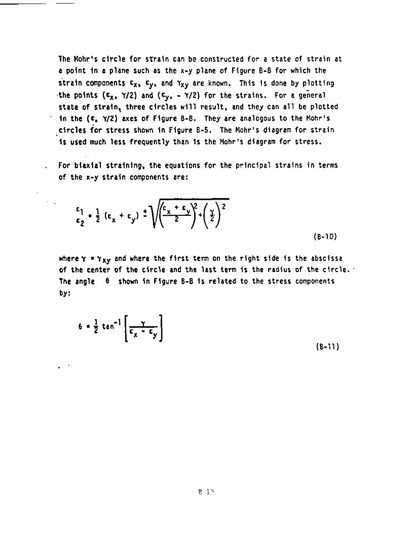
The Mohr's circle for strain can be constructed for a state of strain at
a point in a plane such as the x-y plane of Figure B-8 for which the
strain components cx, cy, and Yxy are known. This is done by plotting
the points (x, Y/2) and (, - Y/2) for the strains. For a general
state of strain, three circles will result, and they can all be plotted
in the (C, Y/2) axes of Figure B-B. They are analogous to the Mohr's
circles for stress shown in Figure -5. The Mohr's diagram for strain
is used much less frequently than is the Mohr's diagram for stress.
For biaxial straining, the equations for the principal strains in terms
of the x-y strain components are:
c * (cx + Cy) +
(B-10)
where Y * Yxy and where the first term on the right side is the abscissa
of the center of the circle and the last term is the radius of the circle.
The angle 0 shown in Figure B-8 is related to the stress components
by:
6 tan]
(B-Cl)
P I,
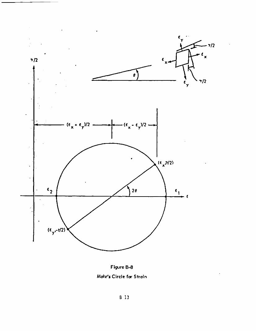
y
I1I2
((x + y V2
'v/2
iC (Xxx
9 ^12y
la ( - V -*
x y
Figure BM8
Mohr's Circle for Strain
(f y,- /2)
B 13
APPENDIX C
MATERIAL YIELD CRITERIA
The state of stress at which yielding occurs is related to the yield
stress for a specimen in a simple tensile test by yield criteria. These
equations prescribe means of determining how close the material's state
of stress, at a point, is to yielding. The state of stress that is com-
pared to the yield stress can be used as a generalized stress condition
for design. It would be legitimate to use it to indicate when the state
of stress reached a magnitude equivalent to a design criterion such as
75% of the yield stress in a uniaxial tensile specimen.
For ductile metals that are commonly used as structural materials, there
are two reliable and commonly used yield criteria. They are the Tresca
and von Mises criteria. The Mohr-Coulomb criteria is often used to
predict yielding of soils and geologic media.
Tresca Yield Condition
The Tresca criterion, published in 1868, postulates that yielding will
occur at a point when the maximum shear stress at that point is equal to
the maximum shear stress in a tensile specimen at yielding. For simple
tension, two of the principal stresses are zero, and the maximum shear
stress is
Tmax *0.5 a
(C-l)
where
tmax maximum shear stress Cf/k2I
00 a tensile stress in smple tensile specimenat yielding (f/k I )
C I
-
The shear stress at a point for any stress state is determined from theprincipal stresses as
Tmax 0.5 max (o - 2;I02 - o3kIl3 - all)
(C-2)
Equations C-I and C-2 are a statement of the Tresca criterion. They can
be combined to eliminate tmax and give a relationship between the absolutevalue of the maximum difference in principal stresses and the yield
stress for a uniaxially loaded tensile specimen.
O= max (1 - 021;102 - 3 1;Io 3 - Il)
(C-3)
Since the Tresca criterion is stated in terms of the principal stresses,the principal stresses must be determined in terms of the stress compon-ents. Either the equations given in Appendix B for biaxial stress, theMohr's diagram methods (biaxial stress) or Equation 3.34 (triaxialstress) may be used to determine the principal stresses.
von Mises Yield Condition
The von Mises yield condition, developed in 1913, states that yieldingwill occur at a point when the state of stress at that point reaches avalue as prescribed by the von Mises formula which is equal to the ten-
sile stress in a simple tensile test at yielding:
0o (GI [t - 02)2 + (2 - 03)2 (3 - O)2]
(C-4)
C 2

where
01, 02, 03 principal stresses in the stress field (fit2)
co tensile stress in simple ten ilespecimen at yielding [f/.tl
The Tresca and von Mises yield surfaces for ductile metals are shown in
Figure C-1 in the Haigh-Westerr:ad stress space looking in along the
hydrostat, which is a line pacing through all points where 1 02
03. The Tresca yield surface projects as a hexagon on planes normal to
the hydrostat. The von Mises yield surface projects as a circle on this
plane and has a diameter equal to the major diameter of the hexagon.
These yield surfaces indicate that yielding occurs at the same stress
magnitude in compression as in tension. These yield surfaces are inde-
pendent of position along the hydrostat and are thus independent of the
hydrostatic state of stress.
Mohr-Coulomb Criterion
For compressible soil type media (e.g., bentonite backfill), yielding is
reasonably well described in terms of the Mohr-Coulomb failure criterion.
This yield criterion relates shear stress on a plane to the normal stress
on the same plane. The criterion can be stated as
By C + n a(n5)
where:
Ty ' shear stress at yield on shear plane [f/t 2]
c cohesion force per unit area [f/P.2)
On normal compressive stres5 on shear plane when yieldingin shear occurs (f/kd3
6 material internal angle of friction [ 1
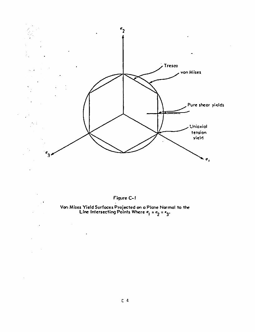
a2
i
I
-1-1
3
jTrescovon Mises
F
Pure sheor yi elds
Unioxialtension
yield
elo
Fiqure C- I
Von Mises Yield Surfoces Projected on a Plone Normol to theLine Intersecting Points Where a, = 2 = r3.
C 4