1

Corruption in Health Sector: Evidence from Unofficial Consultation fees in Bangladesh

Wahid Abdallah, University of Washington

Shyamal Chowdhury, University of Sydney

Kazi Iqbal, World Bank Institute

This Version: 30th September, 2009

Abstract We study the incidence and extent of 'extortion' payment made to the doctors in public health facilities using a nationally representative Household Income Expenditure Survey (HIES) of Bangladesh. A key advantage of using HIES is that it is free from any reporting bias which otherwise occurs in surveys designed purposely for studying corruption. Though consultations are free in public health facilities, HIES data shows that a large number of patients visiting public health facilities have paid fees. We focus on three set of variables to explain incidence and extent of doctor's extortionary power: relation-specific expenditures of patients (transportation cost and travel time), ability of patients to pay (annual income and land ownership), and market power of doctors in public health facilities (proxied by number of total persons engaged in the major health facilities in a community). We found that all three sets of variables are statistically significant in explaining the incidence of corruption, even though travel variables have a negligible effect on incidence of corruption. Furthermore, travel variables and total persons engaged significantly explain the amount of extortion payments in the form of consultation fee whereas the income and wealth are not robust in explaining extortion payments. Consistent with the hold-up theory, high likelihood of extorting payment deter patients visiting public health facilities.

Keywords: Corruption, Public Sector, Public Health, Price Discrimination, Publicly

provided goods, Hold-up problem

JEL Classification: D73, I18, L11, O17, H42

2

I. Introduction

What is the extent of corruption in public sectors and who pays how much of it remain

important questions for policy makers in rich and poor countries (WDR, 2004). However,

due to the inherent difficulty of measuring illegal activities such as corruption, the most

evidences on the incidence and magnitude of corruption rely heavily on perception based

indices, which are subjective by their nature and have obvious limitations.1 Absent

factual measurements of incidence and magnitude, there could be little consensus on how

to reduce corruption and where to allocate efforts for corruption reduction. In this paper,

we use objective measures of the incidence and determinants of corruption in public

health services in Bangladesh using micro level data.

Public health services are important components of public services in general and health

services in particular in Bangladesh. Like many other developing countries, most of the

basic public health services including consultation with doctors at public health facilities

are free in Bangladesh. However, charging fees for such services is very widespread

(Transparency International, 2006)2. For instance, in Bangladesh about 44% patients who

visited public health facilities had to pay consultation fee to the doctors in 2005 with

mean payment of 44 taka and standard deviation of 103 taka3. Thus, questions arise: Who

pays this ‘fee’ and who doesn’t? Why some patients are paying more than others? Do

fees deter (hold-up) patients from visiting public health facilities?

Using nationally representative Household Income and Expenditure Survey (HIES) of

2005 for Bangladesh, we address these two questions. 2005 HIES collected detailed

information on expenditures on different goods and services including health. The section

on health related expenditure includes the amount of money spent for doctor consultation,

1 See Rose-Ackerman for a survey of this literature. Svensson (2003), among others, discusses the shortcomings of perception based cross-country studies. 2 The Transparency International (TI) made health sector as their main theme for their Global Corruption Report in 2006 where a whole section was devoted to informal payments. The report, for example, reveals that 84% of total health expenditure can be attributed to informal payments whereas it constitutes half of total out-of-pocket expenditure in Georgia, the major component (70% – 80%) in health expenditure. Similar practices exist in countries like Russian Federation, Poland, Tajikistan and Albania. The report also presented evidence this kind of payment is also quite prevalent in countries like Slovakia, Latvia, Bulgaria and Romania. 3 Calculated from 2005 HIES. $1 = 69 Taka.

3

other related fees and information on whether the patient visited public or private doctors.

These information allow us to identify unofficial payments made to the doctors which is

free from any reporting bias. In this study we explain the factors that determine the

incidence and the extent of these unofficial ‘fees’ made in public health facilities and if

the likelihood of paying such fees deter some patients.

Our paper is related to the recent growing applied microeconomic literature that

quantifies corruption using micro level data. The central issue of this new literature has

been measuring leakages of public expenditure allocation, explaining the efficiency of

public service providers and probing the incidence and extent of corruption based on the

characteristics of recipient of the public services (e.g., household and firm)4.

Svensson (2003) was perhaps the first to analyze unofficial payments on cross section of

firms in Uganda where he found that firms on which public officials has more control

(measured by indices developed by the author) has a higher probability to pay whereas

firms with a higher ability to pay (proxied by current and future profitability) and lower

refusal power (proxied by estimated alternative return on capital) had to pay more due to

weaker bargaining power. Similarly, Hunt (2007) analyzed unofficial payments in health

care sector in Peru and Uganda and found that richer patients are more likely to pay

bribes as well as pay more. Both Svenson (2003) and Hunt (2007) use data set that

contains quantitative information on bribe payments, where respondents were asked how

much they had to pay to get access to services (customs, licenses, electricity, telephone

etc in Svenson’s case and healthcare in Hunt’s case). While they are informative, the

direct reporting on bribes can lead to under or over reporting depending on the bribe-

payer’s objectives, which our data is free from.5 In addition, Svenson (2003) has a large

number of missing bribery data (27.5%) where firms refused to report on bribes paid

which raises the issue of selection bias (which confirms Bertrand et al (2006) observation

quoted above).

4 see Reinikka and Svensson, 2003 for detail 5 In discussing about the need of micro data regarding corruption, Bertrand et al (2006, p.29) mention that “Had we ran a survey simply asking individuals who had obtained a license whether they paid bribes, we have had concluded that there was no corruption in the bureaucratic system.”

4

Other relevant studies for the current purpose are Banerjee, Deaton and Duflo (2004),

Bertrand et al (2006), and Olken and Barron (2007). Based on survey data collected from

one district in rural Rajasthan in India, Banerjee, Deaton and Duflo (2004), who

evaluated the impact of access to health care on well being, also reported incidences of

informal payments in public health facilities. Bertrand et al (2006) in the context of

obtaining driving license in New Delhi in India have focused on regulations and

bureaucratic corruption and found that the bureaucrats respond to private needs; they

(bureaucrats) however ignore socially important components of regulatory objectives.

Olken and Barron (2007) using a survey in combination of a natural experiment have

examined how the extent of corruption changes with a change in market structure and

found that the market structure has an impact on the total amount of bribes charged. In

addition, their findings also support the standard hold-up theory.

In this paper, unlike the existing literature, we have overcome biases created by the

“direct reporting” on bribes and un-representativeness of samples by using a nationally

representative sample that was collected for measuring living standard. None of these

papers however have used a nationally representative as well as household survey as we

did in this paper. Furthermore, our data are collected by Bangladesh Bureau of Statistics,

the public organization responsible for statistical data collection in the country.

We have found that, relationship specific expenditures of patients – transportation cost to

travel to health facility in this case – increase the unofficial consultation fee consierably.

However, the travel variables do not explain incidence of corruption significantly. The

positive effect of travel variables in explaining higher unofficial fees lends support for

hold-up problem (Grossman and Hart, 1986).

We have also analyzed the effect of changes in market power of the public doctor on the

unofficial consultation fee. It turns out that Reduction in doctors’ market power, as

captured by higher number of staffs in public hospitals, is found to reduce the incidence

as well as amount of unofficial payment. Greater number of doctors and staff enhances

5

competition and collusion becomes harder which reduces unofficial payment and the

incidence of corruption.

The rest of the paper is organized as follows. Section II sets up the institutional

background, Section III briefly discusses the conceptual framework for the factors

determining the bargaining process and section IV presents the empirical model and data.

Section V discusses the results on the incidence of corruption and the extent of

corruption. Section VII draws conclusion.

II. Institutional Background

Government of Bangladesh aims to provide basic health care services that include

reproductive health care, child health care, communicable disease control, limited

curative care, and behavior change communication. A considerable amount of these

services including consultation with doctors and provision of some essential medicines

are provided for free at the public health facilities.

The public health facilities are located based on the administrative layout. For

administrative purposes, the country is divided into 6 divisions, 64 districts and 508 sub-

districts. At a lower level, there are 4466 unions in rural areas and 2300 wards in urban

areas. All the divisional and district cities and sub-district towns have public hospitals. At

a lower level, however, not all the unions have public health facilities. More specifically,

there are only 1362 Union (Health) Sub-Centers (USCs) which mostly provide curative,

preventive and family welfare services at the union level. These USCs have four

sanctioned posts with one doctor. There are also 17 Rural Health Centers which are 10

bedded and has 20 sanctioned posts with two doctors. Finally, there are 35 20-bedded

hospitals located at some unions, which covers only 0.7% of the unions.

At a higher level, the Sub-District Health Complexes (SHCs) at sub-district towns

operate as a hub to the primary health care at the bottom tier of the health administrative

layout. There are 153 50-bedded SHCs and 260 31-bedded SHCs with nine sanctioned

6

posts for doctors including junior consultants and surgeons. These health complexes

provide the first level referral services to the community.6

Beyond the Sub-district, there are District Hospitals located at the District cities that

provide second level referral services. These are usually 100 bedded Hospitals, but some

(nine) of these are also 250 bedded (these are called General Hospitals). A greater

number and lines of consultative services are provided at these facilities. A few other

districts also have public medical college hospitals and specialized hospitals as well. All

these health facilities provide secondary as well as tertiary level health care.

At the divisional level, there are no public hospitals as such, but the divisional cities have

at least one medical college hospital with some divisional cities even have specialized

hospitals (these are chest, leprosy and infection disease hospitals) and institute (research)

hospitals. Most of the Medical College Hospitals located at Divisional cities are at least

500 bedded and provide tertiary level health care services. There are also post graduate

hospitals, school health clinics and urban dispensaries.

It is clear from the above that patients in large cities have better access7 to the public

health services than smaller cities and the smaller cities have better services than rural

areas. Furthermore, most unions do not have a USC and therefore, the patients in those

unions need to travel out of the unions if they wish to travel to a public health facility. In

addition, evidence shows that the staffing norm in SHCs and USCs are much different

from actual staffing situation: 68% of USCs do not have a doctor and the mean number of

doctors at SHCs is 5.35.8 This indicates that the access of patients in rural areas varies

considerably and so does doctor’s market power.

6 Note that the total number of SHCs is less than total number of sub-districts. The reason is that each district head quarter, located in the city, also contains a sub-district and therefore, there is no SHCs in these district head quarters since they already have a Sadar or General Hospital. 7 Not necessarily in per capita term. 8 See Final Report of Social Sector Performance Survey: Primary Health and Family Planning in Bangladesh (2005).

7

The sub-districts in general are not very large geographically (the average size of a sub-

district is 290 square km) and there are different forms of transportation available to an

individuals. Anecdotal evidence suggests that commuters mostly use slow, non-

motorized vehicles or simply walk to the sub-district towns from most unions. There are

also motorized vehicles, both public and private, available to the individuals in many

unions. As can be expected, the options of motorized vehicles are larger for unions that

are located on the road linking two large cities..

The number of patients at each type of hospitals is given in the table in appendix 1. The

average number of patients is greater at larger hospitals (in terms of beds, for example).

However, if we consider the total number of patients, then we see that 48.8% of all the

patients visiting public hospitals visit Sub-District Health Complexes and 32.5% go to

Union Sub-Centers. This indicates that SHCs and USCs serve a very large part of the

health market and can have significant market power and associated consequences over a

large population.

III Analytical framework

In this section we present an analytical framework that helps to understand the incidence

and magnitude of corruption and the hold-up possibility. It should be seen as providing a

background to our empirical investigation and the types of behavior that we are interested

in investigating.

When an individual gets sick or injured, he faces a multitude of options such as

consulting doctors in private health facility or in public health facility, or taking

traditional medicines etc. We abstract from these, and focus on choosing between not

seeking treatment and visiting a public health facilities. If the agent decides not to seek

treatment, the expected utility is u(l) while if the agent decides to visit a public health

facility, the expected utility is u(h). However, visiting a public health facility requires

incurring a cost F.

8

Our analysis proceeds in several steps. We consider a two-period model where in period

1, the agent forms expectation about F based on his prior experience, and information

available in the neighborhood. Based on these, the agent decides if to seek treatment in

period 2. We treat u(l) and F as given and consider the role of agent specific

characteristics (income and type of sickness) in seeking treatment. Second, we informally

discuss the role of bribe in our setting and argue that our empirical results imply patients’

likelihood of visiting public health facilities decreases with bribe and increases with his

bargaining power. Third, we consider the possibility of hold-up due to F and bribe.

Assume that in period 1, a patient can make a fixed, non-contractible investment at cost

F, which is given by an indictor variable I, which equals 1 if the patient invests and 0

otherwise. In period 2, there is a potential gain g(I) from going to a public health facility

where g

(1) 1

0 0

G if I

if Ig

=

=

�= ��

We assume G > F (otherwise, no patient will visit public health facilities).

Assume that both doctor (D) and patient (P) make a simultaneous claim, [0, ]iu G∈ , and

the gain G is divided through Nash bargaining, and the payoffs are given by:

(2) ;

0

i D Pu if u u G

otherwiseg

+ ≤�= ��

Here, any combination of uP+ uD = G is an efficient equilibrium. The normal form of the

whole game can be described by the set of pure strategies SP = {0, 1} * [0, G] and SD =

[0, G] and the payoff functions for the patient and the doctor are given by:

9

(4) 1 ;

1 ;

0 0

P D P

D P

u F if I and u u G

P F if I and u u G

if I

s− = + ≤

− = + >

=

��= ���

and

(5) 1 ;

0 0

B D Pu if I and u u G

Dif I

s= + ≤

=

�= ��

The following two equlibria are of particular interest:

Equilibria I: A set of efficient equilibria is given by I=1 in combination with any pair of

claims (sP, sD) such that sP + sD = G and sP � F.

Equilibria II: A set of inefficient equilibria is given by I=0 in combination with any

claim by the doctor sD � G – F and a corresponding claim by the patient G – sD.

Discussion of Equilibria I: Determinants of equilibrium sD

In this case patients visit public health facilities and the pay-offs are allocated through

bargaining between patients and doctors. The determinants of the bargaining power, more

specifically, the equilibrium allocation of G between sP and sD, warrants further

elaboration. In our analysis, we are particularly interested in explaining the

determination of sD, which is the unofficial payments made to the doctors.

The bargaining power of the patient typically depends on income, education, type of

diseases, distance from health facilities, transportation cost and other unobservables,

whereas, for the doctors, it depends on the competition from other doctors in the

neighborhood, both private and public.

We first consider income and wealth of a patient as determinants of his/her bargaining.

An increase in Income of the patients increases the willingness and ability to pay for fees

and it may weaken their bargaining power. Though the doctors don’t have the income or

wealth information at the beginning, this information may be revealed through

10

appearance and conversation, and repeated interactions. On the other hand, doctors may

not ask for unofficial fee from a well-off person who can be socially well connected.

Moreover, land rich persons in rural areas are often influential and may not be charged

any fees because the local doctors may want to maintain good relationship with them.

Therefore, income and wealth effect on the incidence and extent of unofficial payments

made to the doctors are not very obvious.

Severity of health shock such as critical diseases and its extent of urgency can also affect

patients’ bargaining power. In case of emergency, patients can be expected to seek

immediate attention of the doctors and therefore, may be less reluctant to bargain with

doctors. On the other hand, some diseases by nature may result in lower bribe payment.

For example, in case of chronic diseases which require frequent visits by the patients,

doctors and patients may develop a relationship through frequent meetings and doctors

may charge less, if not zero.

Every patient needs to make a certain amount of effort (e.g., time and cost to reach

hospital), in order to reach the health facility for treatment. In the event a fee is charged

for the service, a patient may disagree to do so since it is illegal. However, disagreeing to

pay may also cost the patient by not getting the service. In that event, the patient not only

loses the service but the effort made to reach the facility also becomes sunk. Furthermore,

this cost is higher if the effort made is higher. Hence, the patient with greater effort will

have a lower bargaining power and may end up paying more.

Individual characteristics such as patients’ age, sex and religion may also play role in the

bargaining process. Young, female and minority groups may have lower bargaining

power and end up paying more. However, when young and female patients are

accompanied by adult and male, which is very likely in developing countries, this

argument will not hold.

The bargaining power of the doctors hinges heavily on their market power in their local

health services market which in turn depends on availability of other health facilities,

11

both private and public. Wilson (1989) in his celebrated work suggested that a greater

number of service windows limit the ability of bureaucrats to charge extortion since

individuals can always switch to a different window if such a charge is made. In our

context, a larger number of doctors increases competition among the doctors in a public

health facility and also makes it harder to collude. We can therefore expect that increased

number of doctors should reduce consultation fee.9

Discussion of the equilibria II: Hold-up problem

In this case patients are deterred to visit hospital as their initial cost to reach the facility

and the doctor’s claim (unofficial fees) are too large to cover their benefit from the health

care. Transportation cost incurred and time spent to reach a public health facility can

make patients vulnerable to ex-post exploitation by health service providers. In rural

areas where public health facilities are dispersed and private health facilities are limited

in supply, patients after arriving in public health facilities can potentially be held up by

doctors. If patients know it, we would observe too few sick people visiting public health

facilities. This is an example of the standard hold-up problem (Grossman and Hart,

1986).

The information set available to the patients about the distribution of doctor’s fees can be

an important determinant of the hold-up problem. If the patients know about the higher

fees of the doctors before visiting the public hospital, they may not visit at all. This

information is typically gathered by previous personal experiences and from the

neighborhood.

9 Furthermore, non-doctor staffs in public health facilities often play an important part in the whole bargaining process,

especially in organizing these payments. Assuming that these staffs get a share of the payment, a larger number of

staffs increase competition among the staffs to serve the doctors. This reduces bargaining power of the staffs and hence,

the share paid to the staffs. This lowers the cost of organizing the payment and doctors would charge patients less.

Since doctor’s consultation is now cheaper at this facility, doctors at other public health facilities in the same sub-

district can be expected to face a lower demand and may lower their (unofficial) fees too.

12

IV. Empirical Framework

Following the two set of equilibrium described above, we first study the determinants of

the incident and extent of corruption (Equilibria I) and the determinants of the hold-up

problem (Equilibria II). We observe three outcomes in our data set for agents who get

sick: 1) opt for public health care and pay bribe; 2) opt for public health care and do not

pay bribe; 3) do not seek treatments. According to our analytical framework, outcomes 1

and 2 are linked to the first set of equilibria, and outcome 3 is linked to the second set of

equilibria. We treat the outcomes in a discrete choice framework (McFadden 1974) and

assume that patients make a choice from the above three outcomes j. The utility that the

ith patient derives from choosing the outcome j consists of two components, a systematic

component and a random component, and can be expressed as:

(6) ij ij ijU G ε= +

Here Gij is the systematic portion of the utility function, which can be viewed as the

‘gain’ discussed in our analytical framework. As discussed, the net gain is determined by

F, healthcare specific characteristics (availability of alternative suppliers etc) and patient

specific characteristics including income, demographic and sickness. ijε is a stochastic

element.

Assuming that patients maximize their utility, the choice problem involves a comparison

of utilities associated with each of the j alternatives, and a rational agent makes choices

among different alternatives that yield the maximum utility. Let Yi be a random variable

that denotes the choice outcome, then the probability that individual i chooses j is given

by:

13

(7) Pr( ) ( )i ij ij ik ikY j P G Gε ε= = + > + for all k=1, …j; k�j

The mapping from a probabilistic choice model to an econometric model of choice is

conceptually straightforward. For the first set of equilibrium, we consider the two discrete

outcomes and estimate a logit model. We consider the extent of bribe and estimate a tobit

model. For the second set of equilibrium, all three possible outcomes and estimate a

multinomial logit model.

We estimate several commonly-used models to estimate patients’ choice among

alternatives. The models vary in their ability to relax the independence of irrelevant

alternatives assumption, in allowing for non-constant variances across varieties and

subjects, and also in computational complexity.

Universal logit

In the universal logit model, the probability that patient i chooses alternative j is given by:

(8)

1

exp( )Pr( )

exp( )

iji J

ijj

GY j

G=

= =�

Where,

ij j i i i iG a b X c Z′ ′= + +

Here j=1…3, i=1…n, aj is choice specific constant, Xi is a vector of observed patient

specific characteristics including F as well, and Zi is vector of observed facility specific

characteristics. A subject chooses Uij if Uij>Uik for all other k possible choices. It is

assumed that ijε is independent and follows a type 1 extreme value distribution given by

exp[-exp(- ijε )] which assumes that the omission of an irrelevant choice set should not

change the parameter estimates.

14

Unlike multinomial logit model, the universal logit model specified above relaxes the

multinomial logit’s cross elasticity properties by including attributes of competing

alternatives in the utility function for all alternatives in the choice set (McFadden, Train

and Tye, 1978). The appearance of significant cross-effects of alternative k would imply

that the utility of an alternative i depends on the attributes of other alternative(s); this is

therefore a test of the independence of irrelevant alternatives (IIA) assumption.

Multinomial probit

The multinomial probit (MNP) model does not assume errors are independently

distributed across alternatives. The probability that subject i chooses alternative j is given

by:

(9) 1Pr( ) ... ... ( ) ...j j k j j JG G G G

i jY j f d dε ε

ε ε ε+ − ∞ + −

−∞ −∞ −∞= =� � �

where J are the alternatives and ( )f ⋅ is a J-variate normal density function with mean

zero and J J× covariance matrix Σ (Louviere et al 2000).

Models specified above have been estimated by using maximum (simulated) likelihood

(Train 2003).

�

For patient specific characteristics Xi, we use individual specific health shock and health

endowment by including types of diseases (chronic, cardio-vascular or respiratory,

infectious or communicable, physical problem, female disease), number of diseases

(patient has two diseases, three diseases), age and gender. We also include household’s

income and land endowment, patient’s status within the household (household head or

not), whether head of household is female, and religion. Also there are no direct proxies

15

available for initial health endowment and other health inputs. Income variables can

partly capture these variables.

Community characteristics of the patient are captured by rural-urban dummy10 and the

percentage of patients visit public health facilities.

For variables that determine F, we include travel time and transportation cost. For

patients who do not attend public health facilities, we use the relevant village averages.

Two variables are used to proxy market power of the doctors: Total persons engaged in a

sub-district hospital and total number of persons seeking treatment in a union. Note that

there is no data available for the quantity of medical services (e.g., time spent on a

patient).

Data

We have used two sets of data in this paper: i. Household Income Expenditure Survey

(HIES) conducted by Bangladesh Bureau of Statistics (BBS) in 2005, and ii. Directory of

Health and Social Welfare 2005, published by the BBS. The HIES 2005 was done on

10,080 households and 48,969 individuals in 518 unions, 366 sub-districts and all the 64

districts. The survey contained income, employment and expenditure modules in addition

to demographics, health and education modules.

In the Health module, the households were asked about type of illness, type of doctors

consulted (whether public or private), travel time and mode of transport. In the health

expenditure module, the households were asked about cost of getting the health service

by simply asking “What was the cost of treatment during the past 30 days?” under which

there are subsections where households need to report the consultation fee,

hospital/clinical charges, cost of medicine, cost of test/investigation, transportation cost,

tips and other charges. These questions were asked irrespective of whether the patient

10 In Bangladesh variations in terms access to water, sanitations, weather etc are negligible within rural and urban regions.

16

went to a private facility or public facility or consulted traditional or spiritual health

professionals.

2005 HIES shows that there were 12,894 individuals who were suffering in either chronic

or non-chronic disease. Among them, 8,573 individuals reported to be suffering from

some kind of illness or injury in past thirty days whereas around 6,314 individuals were

suffering from some sort of chronic illness or disability in past twelve months. However,

not all these individuals sought treatment. In fact, the survey asked whether the individual

had consulted anyone for the illness/injury only. It turns out that there were about 5,874

individuals who consulted someone for the illness/injury they suffered in past 30 days.

Not all the patients seeking treatment visit public hospitals. In fact, most patients do not

visit public health facilities for consultation. Only 619 individuals out of 5, 874 patients

seeking treatment visited public health facilities for doctor’s consultation. However, some

of these patients also visited other facilities too, before or after visiting a public health

facility and there is no way to separate the two consultation fees. We therefore drop these

observations for our analysis which left us with 484 observations.

Data on health facility specific characteristics came from the Health and Social Welfare

Directory 2005 which includes all the health and social welfare organizations that employ

more than 10 persons. The directory contains the name and address of the facility, total

persons engaged, total female persons engaged and year of establishment. The data on

Total persons engaged in public Hospitals beyond Union Health Centers are collected

from here. The Union Health Centers were left out of this directory since these centers

employ less than 10 persons.

How different are the patients visiting public health facilities from all the patients seeking

treatment? Table 1 presents a comparison of these two types of patients on all the

variables that we have considered in this paper. The table reveals that the two groups are

very similar in their economic and demographic characteristics. The mean annual income

for all patients, for instance, are lower than that of patients going to public health

17

facilities, but these patients on average are wealthier since they have higher mean acres of

land. Furthermore, proportion of all patients living in rural area is larger than that of all

patients going to public health facilities.

Table 2 gives some more descriptive statistics of the patients who go to public health

facility as well as those patients who go to public health facility and also pay a

consultation fee to the public doctor. A patient traveling to a public health facility spends

about 57 taka and the trip takes about 38 minutes on average. If only the patients that

made a payment are considered, these numbers go up to 85 taka and 45 minutes. Whereas

this may indicate that these transport variables may have some explanatory powers of

unofficial payments, patients making payments also have higher income and wealth. This

could then mean that richer patients (with higher income and land) may choose more

expensive and faster transports and pay more often too. Indeed, among the patients who

make some kind of payments, a greater proportion choose some form of transportation

(therefore, having positive transportation cost) instead of walking. Since the mean travel

time is also higher, this may also imply that these patients are more likely coming from

further distance.

We use Total Persons Engaged (TPE) in Sub-district Health complexes as an aggregated

number of doctors and staffs working in those complexes which we collected from the

Health Sector Directory 2005 compiled by Bangladesh Bureau of Statistics (BBS). Given

that Sub-District Health Complex (SHC) operates as the local hub to provide the primary

health care and indeed, 49% of all patients availing the public health services do so at

these health complexes, SHCs play an important role11. Since the decisions for how many

persons to work on these health complexes come from the government and not market,

TPE can be thought to be fairly exogenous.

11 Table 2 reveals that the average number of staffs working in a Sub-District Health Complex is around 74,

and even more important, the standard deviation is 65. This implies we have enough variation in total

persons engaged to use it for our analysis.

18

We use aggregated number of treatment seeking patients in each sub-district in the survey

as a proxy for the market size in each sub-district. Since the survey is a stratified-random

sampled, we believe the proxy should perform well.

V. Results and Discussions

Incidence of Corruption: Who Pays Illegal Fees?

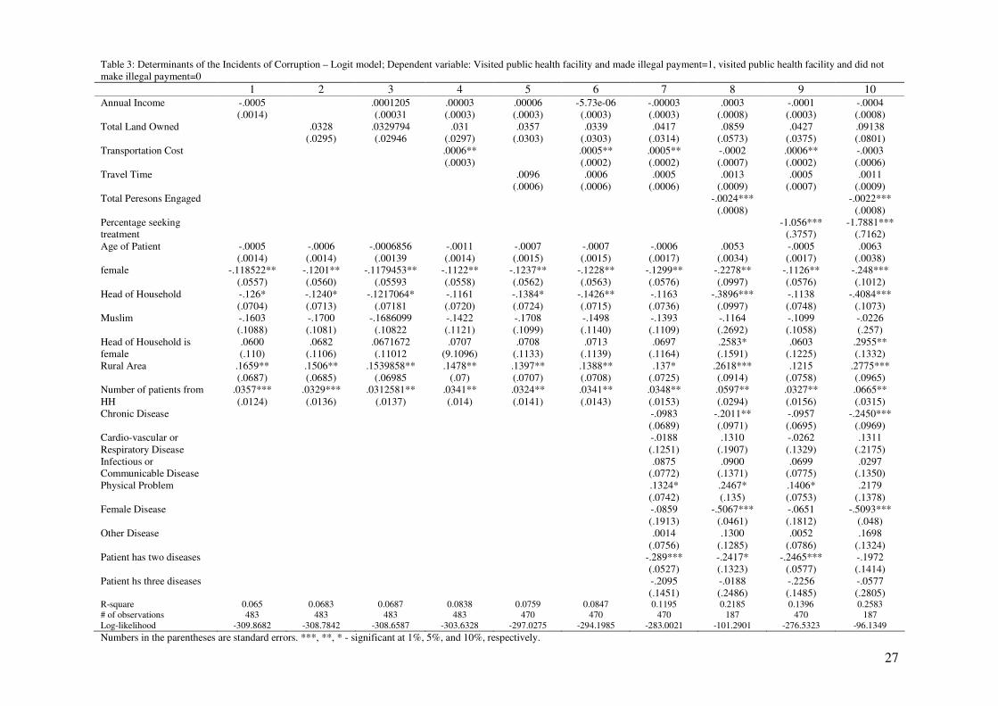
Results estimated through logit model are reported in Table 3. In column 1, 2 and 3, we

consider annual income and total land owned separately and then together where we

control for demographic characteristics. We then add transportation cost and travel time

separately and then together in columns 4, 5 and 6 respectively. In column 7, we

introduce disease related control variables. Finally, in column 8, 9 and 10, we include

total persons engaged and percentage of households seeking treatment and then together

respectively.

First consider the effect of income and wealth of the households on incidence of

consultation fee. Column 1-3 of Table 3 shows that annual income or land-owned do not

explain the probability of making a payment significantly. This pattern remains the same

when all other variables are added in columns 4 through 10.

Second, consider the demographic characteristics. Columns 1 through 10 depict that both

the female dummy and number of patients in a household are statistically significant at

least at 5 % level in all specifications. The sign of the coefficients of these variables

imply that it is more likely that a male patient and households with more patients are

more likely to pay unofficial consultation fee. In addition, the dummy variable for

patients living in rural areas is also statistically significant in most specifications (except

in column 9) and the coefficient is positive. This suggests that patients living in rural

areas have greater probability of paying consultation fee. Finally, the dummy variable for

household head being patient has a negative coefficient which is also statistically

significant in most specifications except the ones in column 4, 7 and 9.

19

We shift our focus next on travel variables. We consider transportation cost and travel

time separately in column 4 and 5 and together in 6 in table 3. We found that a one taka

increase in transportation cost increases the probability of payment by 0.06 percent and it

is statistically significant at 5 percent level. It remained statistically significant at 5%

level with similar magnitude in coefficient even when travel time, disease variables and

percent of households seeking treatment are controlled for in column 6, 7 and 9.

However, the significance of transportation cost vanishes once total persons engaged is

considered in columns 8 and 10. We however find that the coefficient of travel time is not

statistically coefficient in any specification.

Now, consider the disease variables. These include types of diseases, number of diseases

or symptoms the patient is suffering from, whether the patient has a chronic disease and

whether the patient is suffering from any ‘other’ disease. Table 3 shows that no disease

variable has a statistically significant coefficient in all the relevant specifications. The

dummy variable for patients suffering from two diseases or symptoms has a negative and

statistically significant coefficient in three specifications. It is however not significant

when all the variables are considered as in column 10. Furthermore, the dummy variable

for patients having physical problems has a positive and statistically significant

coefficient at 10% level in all specifications except specification 10. Chronic disease, as

expected, has a negative coefficient which is also statistically significant in specifications

whenever total persons engaged in Sub-district Health complex is considered. Dummy

variable for female disease is also statistically significant at 1% level in these

specifications with negative coefficients.

We now turn to the variables that reflect market power of the doctors. Columns 8 and 10

show that total persons engaged in a Sub-district Health Complex has a negative

coefficient and it is statistically significant at 1% level even when the market size is

controlled for. In particular, an additional engagement of one person in a Sub-district

Health Complex decreases the incidence of corruption by 0.24% and 0.22% when market

size is controlled for. Considering mean TPE in a Sub-district Health Complex is 74 and

20

s.d. is 65, this exhibits a significant effect. Note that the inclusion of this variable reduces

the sample size greatly.

The result regarding number of patients seeking treatment in a sub-district is presented in

column 9 and 10 of table 3 with all other controls. The number of patients seeking

treatment is also statistically significant at 1 percent with negative sign. The absolute

magnitude of the coefficient goes up when total persons engaged is included in the

analysis on column 10 whereas the coefficient is still statistical significant at 1% level.

Extent of Corruption: Who Pays More?

We now measure the extent of corruption by using the amount of unofficial consultation

fee with a Tobit model; the results are reported in Table 4. For the ease of understanding,

we follow the exact organization of table 3 in table 4 too.

Consider again income and total land first. Unlike the incidence of corruption, we see that

income has a statistically significant coefficient with positive sign when only

demographic variables are considered. This significance however vanishes when other

variables are added. Total land owned also has a statistically significant coefficient with

positive sign in specification 5 and 7 even though the coefficient is not significant for

other specifications. This may suggest that there may be some income and wealth effect

on determining the level of consultation fee through willingness and ability to pay for

consultation fee.

As far as demographic variables are concerned, no demographic variable is statistically

significant whenever percent of household seeking treatment is controlled for. For other

specifications, it turns out that dummy variable with patients living in rural areas pay

more consultation fee and the coefficient is statistically significant at least at 5% level.

The dummy variable for patients who are Muslims is statistically significant with a

negative sign for all specifications except when disease variables are controlled for.

21

We analyze the travel variables now. Table 4 shows that transportation cost is statistically

significant at 1% level with positive coefficient at all specifications. The magnitude of the

coefficient however declines a bit when total persons engaged in Sub-district Health

Complexes are included. Travel time however is statistically significant only when

transportation cost is not considered. Whenever transportation cost is included, the

coefficient of travel time drops significantly and even becomes negative in some

specifications.

Among the disease variables, number of diseases seems to play a key role in determining

unofficial fee. In particular, the dummy variable with patients having two diseases or

symptoms has statistically significant coefficient at least at 5% level in all the four

specifications and has a negative sign. In addition, the dummy variable with patients

having three diseases or symptoms has negative and statistically significant coefficient in

specifications where total persons engaged in Sub-district Health Complex is not

considered. Dummy variable with patients having physical problems also has a positive

coefficient which is significant in most specifications (except column 8). Finally, the

dummy variable with patients having infectious diseases has positive and statistically

significant coefficient in specifications where total persons engaged in Sub-district Health

Complex is not considered.

The market power indicator – TPE is significant at 1% level and robust with expected

negative signs as shown in column 8 and 10. The market size proxy is also statistically

significant at least at 5% level in all the specifications where it considered (column 9 and

10).

Hold-up: Does bribe deter patients?

Table 5, column 3 shows the determinants of hold-up; why agents being sick may not

seek treatment at all.

Results show that the transportation cost is an important determinant of hold-up problem

and patients who live far from public health facilities are more likely to under-invest.

22

This confirms that patients may consider the possibility that once they arrive in a public

health facility, health providers may ask for bribe over and above the average bribe that

patients pay. As one would expect, this would be more pronounced in rural areas where

patients cannot switch to alternative providers where public health facilities are dispersed,

and private health facilities are limited in supply. This is in fact the case here; the rural

dummy is positive and the coefficient is statistically significant. As a result, two things

are happening – patients who live far or need to spend more on travel are less likely to

visit public health facilities and in addition, and this effect is more pronounced for

patients living in rural area.

Information available to the patient either from his own experience or from the

neighborhood is an important determinant of hold-up. Two variables confirm this finding:

patients with chronic diseases are more likely to visit health facilities, more likely to be

better informed about the likelihood of paying bribe, and more likely to pay less bribe.

However, they are also more likely to decrease their visit frequency due to better

information and more likely to under-invest as a result. Similarly, as more and more

patients visit public health facility from a particular neighborhood measured as a

percentage-sought-treatment increases, neighborhood gets more and more informed about

illegal payments at public health facilities. This again decreases the likelihood of seeking

treatment and leads to underinvestment.

VI. Conclusion

This paper is an important contribution to the growing literature of empirical micro

studies of corruption. It investigates the factors that affect the unofficial payments made

to the government doctors as consultation fees in Bangladesh. Consistent with hold-up

theories, we find that patients having more relation-specific investments, represented by

transportation cost, end up paying more unofficial consultation fees. Furthermore, an

increase in number of total persons engaged in a Sub-District Health Complex, which

imply lower market power of the staff in a public health facility, not only reduces amount

of unofficial fees paid but also the incidence of corruption. However, income and wealth

23

measured by amount of land owned do not significantly explain either incidence or extent

of corruption.

References Banerjee, Abhijeet, Angus Deaton and Esther Duflo (2004). “Wealth, Health and Health Serrvices in Rural Rajsthan.” American Economic Review. Vol 94, No. 2 (May) : 326 – 330. Bangladesh Bureau of Statistics. Bangladesh Health and Social Welfare Directory 2005. Ministry of Planning. Bangladesh. Bertrand, Marianne, Simeon Djankov, Rema Hanna and Sendhil Mullainathan (2007). “Obtaining a Driver's License in India: An Experimental Approach to Studying Corruption.” Quarterly Journal of Economics. Vol. 122 (November): 1639 –1676. Besley, Timothy and Maitreesh Ghatak (2005). “Competition and Incentives with Motivated Agent.” American Economic Review. Vol 95, No. 3 (June) : 616 – 636. Financial Management Reform Program (2005). Social Sector Performance Survey: Primary Health and Family Planning in Bangladesh: Assessing Service Delivery. Ministry of Health and Family Welfare, Bangladesh. Grossman, Sanford and Oliver Hart (1986). “The Cost and Benefit of Ownership: A Theory of Vertical and Lateral Integration.” Journal of Political Economy. Vol 94, No. 4: 691 – 719. Hunt, Jennifer (2007). Bribery in Health Care in Peru and Uganda. IZA DP No. 2757. McGuire, Thomas G. (2000). “Physician Agency.” In Handbook of Health Economics edited by A. J. Culyer and J. P. Newhouse. Elsevier, New York. Olken, Benjamin A. and Patrick Baron (2007). “The Simple Economics of Extortion: Evidence from Trucking in Aceh.” NBER working paper # 12428. Rose-Ackerman, S. (2004). The Challenge of Poor Governance and Corruption. Mimeo. Copenhagen Consensus and Yale University. Svensson, Jakob (2003). “Who Must Pay Bribes and How Much? Evidence from a Cross Section of Firms.” Quarterly Journal of Economics. 118 (February): 207 – 230.

Shleifer, Andrei, and Robert W. Vishny (1993). “Corruption,” Quarterly Journal of Economics. 108, 599–617.

24

Transparency International (2006). Global Corruption Report: Corruption and Health. Germany. Wilson, James Q. (1989). Bureaucracy: What Government Agencies Do and Why do they Do It. Basic Books, Now York.

25

Table 1: Comparison of all the patients and patients going to public health facilities

Full sample of Patients Patients going to public

health facilities

T

statistic

Mean S. D. n Mean S. D. n

Total Income (in thousand taka) 85.543 125.426 5580 95.494 137.34 484 -1.2965

Total land owned (in acres) .895 1.756 5580 .669 1.224 484 0.9598

Age of the patient 24.413 21.662 5579 26.557 21.528 483 -1.9618

Dummy whether a patient lives in rural area .62 .486 5580 .475 .5 484 6.3449

Dummy if the head of household is female .034 .182 5580 .039 .194 484 -0.3083

Dummy if patient is female .508 .5 5580 .519 .5 484 -0.6461

Dummy if household head is patient .207 .504 5580 .231 .422 484 -1.0604

Dummy if the patient is Muslim .9 .3 5580 .893 .31 484 0.4597

Consultation fee (in Taka) 37.781 92.758 5580 43.538 102.9 484 0.8608

Transportation cost (in Taka) 28.221 155.103 5580 56.932 171.652 484 -3.5624

Travel time (in minutes) 26.62 46.22 4739 37.623 54.599 406 -4.1212

Dummy whether patient availed a fast (motorized) transport

.092 .289 5577 .21488 .411 484 -7.5988

Dummy whether patient availed a slow (non-motorized) transport

.345 .476 5577 .5165 .500 484 -7.2493

Dummy whether patient availed any other type (not defined) of transport

.087 .282 5577 .01 .101 484 5.4329

Dummy whether the patient has a chronic disease

.223 .416 5580 .205 .404 484 0.0771

Dummy whether the patient is suffering from a cardio-vascular or respiratory disease

.084 .277 5580 .114 .318 484 -2.8059

Dummy whether the patient is suffering from a infectious or communicable disease

.164 .37 5580 .147 .354 484 0.5175

Dummy whether the patient is suffering from a physical problem

.247 .431 5580 .246 .431 484 1.1818

Dummy whether the patient is suffering from a female disease

.009 .094 5580 .012 .111 484 -0.8781

Dummy whether the patient is suffering from any other disease

.087 .282 5580 .159 .366 484 -1.8862

Dummy whether the patient is suffering from two diseases

.219 .414 5580 .147 .354 484 3.0389

Dummy whether the patient is suffering from three diseases

.044 .205 5580 .027 .162 484 0.7201

Note: We omit education of, say, head of household is a partially ordinal variable and therefore, omitted. More specifically, for numbers 0 to 10, the number represents number of years studied. But above it, it becomes categorical.

26

Table 2: Descriptive statistics of patients going to public health facilities

Variable name Mean S. D. n

Dummy if a unofficial payment is made

.44 .497 484

Payment made as consultation fee (in taka)

43.538 102.9 484

Payment made as consultation fee if only positive payments are considered (in taka)

98.93 136.447 213

Transportation cost (in taka)

56.932 171.652 484

Transportation cost of patients who made positive payments (in taka) 85.005 237.586 213 Travel time (in minute)

37.623 54.599 406

Travel time of patients who made positive payments (in minute) 44.56 64.189 168 Annual Income (in thousand taka)

95.494 137.336 484

Annual income of patients who made positive payments (in taka) 99.849 90.755 213 Total Land owned (in acres)

.669 1.224 484

Total Land owned (in acres) of patients who made positive payments (in taka)

.8615 1.395 213

Total persons engaged in a Sub-District Health Complex 73.979 65.067 194 Dummy whether patient availed a fast (motorized) transport .21488 .411 484 Dummy whether patient availed a slow (non-motorized) transport .5165 .500 484 Dummy whether patient availed ‘other’ (not defined) type of transport .010 .101 484 Note: Fast (motorized) transport includes private car, taxi, bus, auto rickshaw, ambulance, and engine boat. Slow (non-motorized) transport includes rickshaw, non-motorized van, cart, non-motorized boat. The base for all the transport dummies is walking.

27

Table 3: Determinants of the Incidents of Corruption – Logit model; Dependent variable: Visited public health facility and made illegal payment=1, visited public health facility and did not make illegal payment=0 1 2 3 4 5 6 7 8 9 10 Annual Income -.0005

(.0014) .0001205

(.00031 .00003 (.0003)

.00006 (.0003)

-5.73e-06 (.0003)

-.00003 (.0003)

.0003 (.0008)

-.0001 (.0003)

-.0004 (.0008)

Total Land Owned .0328 (.0295)

.0329794 (.02946

.031 (.0297)

.0357 (.0303)

.0339 (.0303)

.0417 (.0314)

.0859 (.0573)

.0427 (.0375)

.09138 (.0801)

Transportation Cost .0006** (.0003)

.0005** (.0002)

.0005** (.0002)

-.0002 (.0007)

.0006** (.0002)

-.0003 (.0006)

Travel Time .0096 (.0006)

.0006 (.0006)

.0005 (.0006)

.0013 (.0009)

.0005 (.0007)

.0011 (.0009)

Total Peresons Engaged -.0024*** (.0008)

-.0022*** (.0008)

Percentage seeking treatment

-1.056*** (.3757)

-1.7881*** (.7162)

Age of Patient -.0005 (.0014)

-.0006 (.0014)

-.0006856 (.00139

-.0011 (.0014)

-.0007 (.0015)

-.0007 (.0015)

-.0006 (.0017)

.0053 (.0034)

-.0005 (.0017)

.0063 (.0038)

female -.118522** (.0557)

-.1201** (.0560)

-.1179453** (.05593

-.1122** (.0558)

-.1237** (.0562)

-.1228** (.0563)

-.1299** (.0576)

-.2278** (.0997)

-.1126** (.0576)

-.248*** (.1012)

Head of Household -.126* (.0704)

-.1240* (.0713)

-.1217064* (.07181

-.1161 (.0720)

-.1384* (.0724)

-.1426** (.0715)

-.1163 (.0736)

-.3896*** (.0997)

-.1138 (.0748)

-.4084*** (.1073)

Muslim -.1603 (.1088)

-.1700 (.1081)

-.1686099 (.10822

-.1422 (.1121)

-.1708 (.1099)

-.1498 (.1140)

-.1393 (.1109)

-.1164 (.2692)

-.1099 (.1058)

-.0226 (.257)

Head of Household is female

.0600 (.110)

.0682 (.1106)

.0671672 (.11012

.0707 (9.1096)

.0708 (.1133)

.0713 (.1139)

.0697 (.1164)

.2583* (.1591)

.0603 (.1225)

.2955** (.1332)

Rural Area .1659** (.0687)

.1506** (.0685)

.1539858** (.06985

.1478** (.07)

.1397** (.0707)

.1388** (.0708)

.137* (.0725)

.2618*** (.0914)

.1215 (.0758)

.2775*** (.0965)

Number of patients from HH

.0357*** (.0124)

.0329*** (.0136)

.0312581** (.0137)

.0341** (.014)

.0324** (.0141)

.0341** (.0143)

.0348** (.0153)

.0597** (.0294)

.0327** (.0156)

.0665** (.0315)

Chronic Disease -.0983 (.0689)

-.2011** (.0971)

-.0957 (.0695)

-.2450*** (.0969)

Cardio-vascular or Respiratory Disease

-.0188 (.1251)

.1310 (.1907)

-.0262 (.1329)

.1311 (.2175)

Infectious or Communicable Disease

.0875 (.0772)

.0900 (.1371)

.0699 (.0775)

.0297 (.1350)

Physical Problem .1324* (.0742)

.2467* (.135)

.1406* (.0753)

.2179 (.1378)

Female Disease -.0859 (.1913)

-.5067*** (.0461)

-.0651 (.1812)

-.5093*** (.048)

Other Disease .0014 (.0756)

.1300 (.1285)

.0052 (.0786)

.1698 (.1324)

Patient has two diseases -.289*** (.0527)

-.2417* (.1323)

-.2465*** (.0577)

-.1972 (.1414)

Patient hs three diseases -.2095 (.1451)

-.0188 (.2486)

-.2256 (.1485)

-.0577 (.2805)

R-square 0.065 0.0683 0.0687 0.0838 0.0759 0.0847 0.1195 0.2185 0.1396 0.2583 # of observations 483 483 483 483 470 470 470 187 470 187 Log-likelihood -309.8682 -308.7842 -308.6587 -303.6328 -297.0275 -294.1985 -283.0021 -101.2901 -276.5323 -96.1349 Numbers in the parentheses are standard errors. ***, **, * - significant at 1%, 5%, and 10%, respectively.

28

Table 4: Determinants of the Extent of Corruption – Tobit model; Dependent variable: Amount of ‘fee’ paid 1 2 3 4 5 6 7 8 9 10 Annual Income .1545*

(0882) .1439 (.0887) .0448 (.0807) .1105 (.09) .0311

(.0835) .0236 (.082)

.1214 (.1336)

.0225 (.082)

.0995 (.1334)

Total Land Owned 11.7316 (7.6272)

10.6426 (7.6427)

9.8911 (6.6071)

12.6247* (7.5285)

10.361 (6.6819)

12.1605* (6.6343)

9.3962 (6.5924)

10.6147 (6.6664

7.965 (6.4696)

Transportation Cost .3682*** (.0439)

.3911*** (.0533)

.4036*** (.0532)

.2642*** (.0868)

.4044*** (.0533)

.2676*** (.0851)

Travel time .4363*** (.174)

.0585 (.1646)

-.0105 (.1631)

-.0385 (9.175)

-.0445 (.1639)

-.1025 (.1735)

Total Person Engaged -.3907*** (.1553)

-.4242*** (.1592)

Persons seeking treatment

-1.143** (.4845)

-1.3541*** (.5289)

Age of the patient .1171 (.5616)

.05332 (.5679461)

.0146 (.5664) -.586754 (.501064)

-.2726 (.5843)

-.3212 (.5211)

-.3669 (.5474)

.521 (.6007)

-.4164 (.5513)

.4562 (.5897)

Female -29.3451 (22.4964)

-31.0528 (22.4955)

-28.6902 (22.4778)

-13.4465 (19.5207)

-26.3824 (22.879)

-21.645 (20.3135)

-22.1271 (19.982)

-18.6613 (21.1326)

-17.8327 (20.1645)

-17.1328 (20.8512)

Head of household -8.8684 (31.5508

-8.8198 (31.6556)

-4.5438 (31.6713)

15.5424 (27.5757)

1.1695 (32.2747)

.435049 (28.7247)

7.643 (28.3332)

-44.2215 (33.9727)

8.3048 (28.5399)

-44.638 (33.5153)

Muslim -79.3176*** (29.3897)

-84.2327*** (29.4719)

-81.2724*** (29.4164)

-40.2644 (26.1159)

-78.5405*** (29.5873)

-44.5973* (26.7557)

-35.8203 (26.3323)

-21.1806 (31.5988)

-33.0092 (26.4591)

-16.3865 (31.1155)

Head of household is female

39.8629 (37.6183)

42.8338 (37.7851)

43.5343 (37.703)

40.3245 (32.6095)

39.9054 (37.9485)

37.897 (33.6069)

37.5054 (33.026)

46.8104 (40.6749)

41.3751 (33.0753)

60.4671 (39.7416)

Rural area 57.1646*** (19.1837)

47.5816** (19.5412)

50.9526*** (19.6366)

43.5367*** (17.0385)

47.2488** (19.7636)

41.902** (17.5434)

39.3012** (17.4885)

41.5343** (18.5005)

29.0046 (18.1079)

27.6947 (19.33)

Chronic disease -22.8736 (21.6806)

-26.9003 (22.762)

-24.2016 (21.7609)

-28.0597 (22.4709

Cardio-vascular or respiratory disease

41.8629 (30.3561)

48.6702 (30.1132)

45.8978 (30.4639)

59.0355** (30.0291)

Infectious or communicable disease

44.5468* (26.3124)

24.4375 (28.0511)

43.7593* (26.4299)

26.4823 (27.6588)

Physical problem 41.9774* (23.1058)

34.2727 (24.3917)

49.5322** (23.428)

45.4385* (24.4449)

Female disease -55.0245 (84.1786)

-568.7599 (missing)

-46.438 (87.818

-575.5784 (missing)

Other disease 10.4529 (25.1431)

20.5507 (27.0539)

17.9539 (25.3697)

35.9452 (27.093)

Patient has two diseases

-130.409*** (29.4113)

-72.4465** (29.5885)

-126.0274*** (29.6759)

-74.1187*** (29.1461)

Patient has three diseases

-116.4533* (60.996)

2.3904 (59.1134)

-132.0611** (61.9043)

-15.3441 (59.3863)

R-square2 .0067 .0065 .0073 .0273 .0092 .0255 .0336 .0392 .0356 .0454 Observations 483 483 483 483 470 470 470 187 469 186 Numbers in the parentheses are standard errors. ***, **, * - significant at 1%, 5%, and 10%, respectively.

29

Table 5: Determinants of hold-up – multinomial logit estimates Paid bribe Not seeking

treatment Annual Income 0.00001 -0.000013 (0.00001) (0.000010) Total Land Owned 0.00083 0.000780 (0.00084) (0.001960) Transportation Cost 0.00011 *** -0.000211 *** (0.00002) (0.000050) Travel Time 0.00006 -0.000157 (0.00006) (0.000120) Percentage seeking treatment 0.02158 -0.151268 *** (0.01872) (0.032270) Age of Patient -0.00007 0.000120 (0.00007) (0.000120) female -0.00349 0.000766 (0.00225) (0.005260) Head of Household -0.00344 0.000289 (0.00266) (0.005930) Muslim -0.00201 -0.003158 (0.00491) (0.007510) Head of Household is female 0.00168 -0.001682 (0.00458) (0.008050) Rural Area -0.00321 0.021919 ** (0.00343) (0.006820) Number of patients from HH 0.00112 ** -0.000874 (0.00053) (0.001050) Chronic Disease -0.08401 *** 0.169469 *** (0.01927) (0.026630) Cardio-vascular or Respiratory 0.08391 ** -0.252791 *** Disease (0.04006) (0.059790) Infectious or Communicable 0.04014 *** -0.093460 *** Disease (0.01538) (0.027410) Physical Problem 0.02524 ** -0.047401 ** (0.01060) (0.016910) Female Disease 0.01858 -0.075651 (0.02359) (0.049790) Other Disease 0.03301 ** -0.089370 ** (0.01411) (0.028260) Patient has two diseases -0.01061 *** 0.015752 ** (0.00197) (0.004630) Patient hs three diseases -0.01386 *** 0.031833 *** (0.00221) (0.003500) r2 0.31 0.31 N 5530 5530 Log likelihood -1352.998 -1352.998 Numbers in the parentheses are standard errors. ***, **, * - significant at 1%, 5%, and 10%, respectively.

30

Appendix

Table A1: Total and average number of patients at different hospitals

Type of Hospitals Number of

Hospitals

Total number

of patients

Average Number

of patients

Estimated total

number of patients

Percentage of

patients

Medical College

Hospitals

10 2764824 276482 3592466 7.8

General Hospitals (250

bedded)

2 209892 104946 944514 2.1

District Hospitals

41 3552924 86657 4072879 8.8

Sub-Districts Health

Complexes

350 19075504 54501 22508913 48.8

Union Sub-Centers

1362 14979600 10998 14979600 32.5

Note: Number of hospitals in each category represents the number of facilities from which this data was available. The total and average number of patients represents number of outpatients in those facilities. The estimated total number of patients is computed by average number of patients × total number of facilities.