correlations and empirical relations between static and
TRANSCRIPT
A-8700 Leoben
DEPARTMENT FÜR ANGEWANDTE GEOWISSENSCHAFTEN UND ERDÖLGEOLOGIE LEHRSTUHL FÜR ANGEWANDTE GEOPHYSIK
Montanuniversität Leoben Peter-Tunner-Strasse 25
Master Thesis
Correlations and empirical relations
between static and dynamic elastic
ground parameters in shallow
geotechnical site investigations
submitted at the
Department für Angewandte Geowissenschaften und Geophysik
Lehrstuhl für Angewandte Geophysik der
Montanuniversität Leoben
From: Tutor:
Harald Pölzl Hon. Prof. Dr. rer. nat. habil. H.J Schön
0435014
Leoben, 20.02.2012

EIDESSTATTLICHE ERKLÄRUNG
Ich erkläre an Eides statt, dass ich diese
Arbeit selbständig verfasst, andere als die
angegebenen Quellen und Hilfsmittel nicht
benutzt und mich auch sonst keiner
unerlaubten Hilfsmittel bedient habe.
AFFIDAVIT
I declare in lieu of oath, that I wrote this thesis
and performed the associated research
myself, using only literature cited in this
volume.
Leoben, 27.02.2012
............................................. ...........................................
Ort, Datum Unterschrift

Acknowledgements
I would like to express my appreciation to Mag. Wolfram Felfer from the Fugro Austria GmbH
for facilitating this paper and to Hon. Prof. Dr. rer. nat. habil. Jürgen Schön, University of
Leoben for his time, his patience and his excellent petrophysical support.
My gratitude also goes to the following companies for providing access to data:
Fugro Geotechnical Division, ASFINAG-Autobahnen- und Schnellstraßen-Finanzierungs-AG,
ÖBB-Österreichische Bundesbahnen AG, 3G Gruppe Geotechnik Graz ZT GmbH and ILF-
Beratende Ingenieure ZT Gesellschaft mbH.
The most special thanks go to Heidemarie, Andreas and my parents for supporting me
during all the years of my study.

Kurzfassung
Die Ermittlung von Parametern wie Young’s Modul, Schermodul und Bulk-Modul ist integraler
Bestandteil geotechnischer Baugrunderkundungen. Statische Methoden, die zeit- und
kostenintensiv sind, liefern auf der einen Seite punktuell Informationen, die einen großen
stress-strain-Bereich abdecken. Dynamische Methoden auf der anderen Seite liefern mit
geringerem Aufwand seismische Geschwindigkeiten aus größeren Volumina, die über die
Dichte einfach mit dynamischen Modulen verknüpft sind, allerdings auf sehr kleine strains
begrenzt sind. Um die Vorteile der beiden Zugänge zu kombinieren bzw. die Nachteile zu
kompensieren wird eine Methode präsentiert die einfache, empirische Potenzfunktionen
benutzt, um statische Moduli aus den dynamischen ab zu schätzen. Der gewählte Ansatz
liefert empirische Gleichungen, die gegenüber linearen Ansätzen eine deutlich genauere
Abschätzung erlauben. Die verwendeten Datensätze enthalten statische Methoden, wie den
einaxialen Kompressionsversuch, den Triaxial-Test, Dilatometertests und dynamische
Methoden wie die spektrale Analyse von Oberflächenwellen, Downhole-Seismik, full
waveform sonic logging, PS Suspension Logging, Crosshole-Seismik und
Ultraschallgeschwindigkeitsmessungen im Labor, angewandt auf karbonatische,
siliziklastische, metamorphe und plutonische Gesteine.
Neben der Modulabschätzung wurde auch mit eher geringem Erfolg eine Abschätzung der
einaxialen Druckfestigkeit nur aus den seismischen Geschwindigkeiten versucht. Um eine
höhere Genauigkeit zu erreichen wurden in einem Beispiel Geschwindigkeit, Porosität und
die Rate der Lastaufbringung zu einem Faktor kombiniert mit dem Ergebnis eines sehr guten
linearen Zusammenhangs der einaxiale Druckfestigkeit mit dem gebildeten Faktor.

Abstract
Determination of parameters like Young’s Modulus, Shear Modulus and Bulk Modulus is
integral part of any geotechnical site investigation. On the one hand well established, but
mostly cost and time intensive static methods offer point measurements of moduli over a
broad stress and strain range. On the other hand dynamic methods provide measurements
of acoustic wave velocities in larger volumes at an arguable amount of time and money that
can be easily linked to very small strain dynamic moduli via density. Making use of the
advantages and trying to overcome the disadvantages of each approach a method for the
derivation of power law empirical relations is presented to estimate static moduli from
dynamic moduli with an improved accuracy compared to conventional linear approaches.
The available data involves static unconfined compression, triaxial and dilatometer tests and
dynamic methods like the spectral analysis of surface waves, downhole seismics, full
waveform sonic logging, crosshole seismics and ultrasonic velocity measurements in
laboratory performed in carbonatic, siliciclastic, metamorphic and plutonic rocks.
Beside the estimation of static moduli a not very successful attempt of estimating UCS from
acoustic velocities only is presented. To increase accuracy of UCS estimation velocity,
porosity and stress rate are considered additionally, leading to an excellent linear relation
between for UCS.

Index
____________________________________________________________________________________________________________________________________________________________________________________________________________
Master Thesis ________________________________________________________________________________ Harald Pölzl
1
Index
Page
1 INTRODUCTION AND SCOPE OF WORK ..........................................................3
2 THEORETICAL BACKGROUND .........................................................................5
2.1 Elastic Moduli – Static Approach................................................................................5
2.1.1 Stress and strain..................................................................................................7
2.1.2 Strength- and failure criteria – A Short revision.................................................11
2.2 Elasticity and elastic moduli – dynamic approach ....................................................12
2.2.1 Waves in and around boreholes I – Body Waves..............................................12
2.2.2 Waves in and around boreholes II - Direct and reflected mud waves, trapped
modes, interface waves.....................................................................................15
2.2.3 Waves in and around boreholes III - Surface waves .........................................16
2.2.4 Velocity Anisotropy............................................................................................18
2.2.5 Shear Wave splitting..........................................................................................21
2.2.6 Physical Influences on wave velocities..............................................................22
2.2.6.1 Lithology, Mineralogy..................................................................................22
2.2.6.2 Density........................................................................................................23
2.2.6.3 Porosity.......................................................................................................23
2.2.6.4 Weathering, Moisture content and Fluid Saturation ...................................23
2.2.6.5 Pressure .....................................................................................................24
2.2.6.6 Temperature ...............................................................................................26
2.3 Correlations ..............................................................................................................26
2.3.1 Velocity correlation ............................................................................................27
2.3.2 Static and dynamic Moduli.................................................................................27
2.3.3 Unconfined compression Strength (UCS) and internal angle of friction ............31
3 AVAILABLE METHODS AND DATA .................................................................34
4 COMPARISON OF DIFFERENT DYNAMIC METHODS....................................35
4.1 Conclusions..............................................................................................................42

Index
____________________________________________________________________________________________________________________________________________________________________________________________________________
Master Thesis ________________________________________________________________________________ Harald Pölzl
2
5 RELATIONS BETWEEN VP AND VS ..................................................................43
5.1.1 vp-vs relations in rocks and consolidated materials............................................46
5.1.2 vp-vs relations in soils and/or unconsolidated materials.....................................51
5.1.3 Conclusions.......................................................................................................53
6 CORRELATIONS BETWEEN STATIC AND DYNAMIC MODULI .....................54
6.1.1 Conclusions.......................................................................................................64
7 RELATIONS BETWEEN UNCONFINED COMPRESSION STRENGTH AND
SEISMIC VELOCITIES .......................................................................................66
7.1.1 Conclusions.......................................................................................................74
8 CONCLUSIONS AND DISCUSSION..................................................................75
9 INDICES..............................................................................................................77
9.1 References ...............................................................................................................77
9.2 Tables.......................................................................................................................79
9.3 Figures .....................................................................................................................79
APPENDIX ...................................................................................................................I
Description of involved methods ........................................................................................ I
Seismic Surface Waves - Spectral Analysis of Surface Waves (SASW) ........................... I
Seismic Surface Waves - Active Multichannel Analysis of Surface Waves (MASW)....... III
Seismic Surface Waves - Refraction Micro Tremor (ReMi), Passive and Interferometric
Multichannel Analysis of Surface Waves (MASW)..............................................V
Borehole Extension Testing .............................................................................................VI
Full Waveform Sonic Log (FWS)......................................................................................IX
PS-Suspension Log (PSSL)............................................................................................XII
Gamma Gamma Density Log........................................................................................ XIV
Downhole Seismic........................................................................................................ XVII
Crosshole Seismic ......................................................................................................... XX
3-Axial and Unconfined Compression Test................................................................. XXIII
Piezo-Element testing (transmission and Bender elements) ......................................XXVI

Chapter 1 – Introduction and scope of work 3
____________________________________________________________________________________________________________________________________________________________________________________________________________
Master Thesis ________________________________________________________________________________ Harald Pölzl
1 Introduction and scope of work
Dynamic geophysical methods become more and more important in geotechnical site
investigations. Especially information about elastic ground parameters including Poisson’s
Ratio, Young’s Modulus, Shear Modulus or Bulk Modulus is of central importance for solving
many tasks related to subsurface engineering or construction work. These parameters can
be obtained by a palette of testing methods which can be classified from different points of
view. Static methods are usually well established in geotechnics. They offer reliable values
for the different moduli over a broad stress and strain range representing different conditions
that are realized during and after design. One problem is, that static methods offer mostly
very localized (mainly point) measurements, that are costly and time intensive.
Geophysical methods on the other hand can be used to obtain moduli at very small strains
and high frequencies via measurement of seismic velocities and density. Their advantage is
that they can cover large volumes at an arguable amount of time and money.
The scope of this work is to find and analyze correlations between static and dynamic
methods and moduli to make use of the advantages of both methods. Reliable correlations
between static and dynamic moduli could help to extend the static information from a
measurement point to a larger volume that was investigated with dynamic methods.
The first part of this report should give a short introduction on the theoretical background
about static and dynamic measurements of ground parameters. It should summarize the
main principles of stress and strain in rocks and soil and also includes the basics of acoustic
wave propagation in the underground and in boreholes. The last part of the theoretical
introduction is about empirical correlations between the different parameters.
As a next step it was planned to compare different static and different dynamic methods
separately with each other to get a feeling how congruent the results of different methods
are. Unfortunately a direct comparison of different static measurements was not possible
because there was too low “data intersection” in the given datasets. Different static methods
have not been performed on the same location, so a direct comparison of this kind of
methods was not possible. For the dynamic methods the direct comparison is presented.
To obtain dynamic moduli from acoustic measurements, beside density compressional and
shear wave velocities are necessary. Shear wave velocity determination is often difficult or
impossible, especially in shallow geotechnical investigations, whereas compressional wave
velocity determination is less critical. Therefore an empirical approach is presented to derive
shear wave velocities from measured compressional velocities in site areas where shear
wave velocity could not be measured.
The main part is built by the chapter about correlations between static and dynamic moduli.
Although generally large datasets were available, the approach of direct correlation (only
moduli from the same location/borehole and the same depth were used for correlations)
decreased the amount of data drastically. According to literature, direct and linear

Chapter 1 – Introduction and scope of work 4
____________________________________________________________________________________________________________________________________________________________________________________________________________
Master Thesis ________________________________________________________________________________ Harald Pölzl
correlations have been tried, resulting in mostly moderate to poor correlations and empirical
equations. For this reason a new approach over power law equations has been successfully
performed to increase quality of correlations.
Due to the fact that in nearly all datasets unconfined compression strength data was
available, the correlation of this strength property with acoustic wave velocities is also
involved in this report. On the one hand it was tried to relate unconfined compression
strength to wave velocities only, and on the other hand it was tried to involve porosity and
stress rate beside the wave velocities to increase the accuracy of unconfined compression
strength estimation.

Chapter 2 – Theoretical Background 5
____________________________________________________________________________________________________________________________________________________________________________________________________________
Master Thesis ________________________________________________________________________________ Harald Pölzl
2 Theoretical Background
2.1 Elastic Moduli – Static Approach
Description of elastic behaviour follows Hooke’s Law. Generalization of Hook’s Law as a
tensor has the form (SCHÖN, 1996):
σik = Ciklmεlm or εik = Diklmσlm (1)
σik stress tensor
Ciklm elastic stiffness tensor or tensor of elasticity
εlm strain tensor
Diklm tensor of compliances
The elastic potential, the independence of elastic energy from strain history and the
symmetry of stress/strain-tensors are responsible for the fact that 21 or less independent
tensor components exist (HELBIG, 1992). In case of an isotropic material only 2 independent
properties are necessary (HELBIG, 1992).
Besides the Lame parameters λ and µ, any pair of two of the following moduli can be used
for a description of the elastic properties of an isotropic material (HELBIG, 1992, SCHÖN,
2011):
- Young’s modulus E, defined as ratio of stress to strain in a uniaxial stress state
- Compressional Wave Modulus M, defined as ratio of stress to strain in a uniaxial
strain state
- Bulk Compressional Modulus K or k, defined as ratio of hydrostatic stress to
volumetric strain
- Shear modulus G or µ, defined as ratio of shear stress to shear strain
- Poisson’s ratio ν, defined as the (negative) ratio of lateral strain to axial strain in an
uniaxial stress state

Chapter 2 – Theoretical Background 6
____________________________________________________________________________________________________________________________________________________________________________________________________________
Master Thesis ________________________________________________________________________________ Harald Pölzl
Table 1 shows a table of useful conversions and transformations for different cases of known
and unknown parameters in an isotropic medium.
Compr. Wave
Modulus
M
Young’s Modulus
E
Shear
Modulus
Lame Constant
Bulk Modulus
k
Poisson’s
Ratio
,E
211
1
E
- 12
E
211 E
213 E
-
,E
E
E
3
4
- -
E
E
3
2
EE
33
2
2E
kE, Ek
Ekk
9
33
-
Ek
kE
9
3
Ek
Ekk
9
33
-
k
Ek
6
3
,k
1
13k
213 k
12
213k
1
3k
- -
,k 3
4k
k
k
3
9
-
3
2k
-
k
k
32
23
,k 23 k
k
kk
39
k
2
3- -
k3
, 2
23
- -
3
2
2
,
21
12
12 -
21
2
21
1
3
2
-
,
1
211
2
21
-
3
1
-
Table1: Table of useful transformations and conversions for different combinations of known and unkown parameters. In
the first column the known parameters are listed, in the first row the parameters that should be calculated with the
known parameters are listed (SCHÖN, 2011).

Chapter 2 – Theoretical Background 7
____________________________________________________________________________________________________________________________________________________________________________________________________________
Master Thesis ________________________________________________________________________________ Harald Pölzl
The stress-strain behaviour of rocks is nonlinear and not really ideally elastic (SCHÖN,
1996). Only intact rocks may react approximately elastic (BARTON, 2007). Hook´s law can
be expanded with time dependant terms, describing for example a visco-elastic material
(SCHÖN, 1983).
Static moduli are based on application of static stress (load per area), the resulting
deformation (displacement between two measurement points) and the derived strain
(deformation divided by the original length) (LAMA, 1978). Axial strain is accompanied by
transverse or lateral strain (LAMA, 1978). Under compression lateral strain is positive and
under tension it is negative (LAMA, 1978).
2.1.1 Stress and strain
In general the mechanical state of a system is defined by the position of each part of the
system, by the forces acting on and between each part and by the displacement of each part
of the system (DE VALLEJO & FERRER, 2011). Stress is the result of acting forces on a
plane (DE VALLEJO & FERRER, 2011). Forces might be tensile or compressive causing
normal stress in a rock or they might be shear forces leading to shear stress (DE VALLEJO
& FERRER, 2011). Strain is defined by the variation in the distance between two particles of
the rock system (DE VALLEJO & FERRER, 2011). In general stress is a combined effect of a
natural stress field and (maybe) of additional, artificial stress (load, excavation,…) (SCHÖN,
2011).
The triaxial stress state for rocks under confining pressure is described best by the maximum
principal stress σ1, the intermediate principal stress σ2 and the minimum principal stress σ3
(MOGI, 2007). The maximum principal stress can be described as a function of the other two
stresses σ1=f(σ2 ,σ3) leading to a surface for a given material (MOGI, 2007). Failure strength,
fracture angle and ductility are the basic mechanical properties defined by the stress state
(MOGI, 2007).
The stress-strain curve (Fig.1) shows different characteristics and parts (MOGI, 2007). The
linear part of the curve is caused by elastic behaviour (DE VALLEJO & FERRER, 2011). At
the yield point linear, elastic behaviour ends and plastic or ductile deformation starts (DE
VALLEJO & FERRER, 2011). The peak strength is the maximum stress that a rock can
sustain (DE VALLEJO & FERRER, 2011). Residual strength is the lowered strength value in
the post peak phase (DE VALLEJO & FERRER, 2011). At Peak Strength brittle or ductile
failure should occur (DE VALLEJO & FERRER, 2011). DE VALLEJO & FERRER, 2011 also
mention long time effects like creep or relaxation. Creep is a process where strain still

Chapter 2 – Theoretical Background 8
____________________________________________________________________________________________________________________________________________________________________________________________________________
Master Thesis ________________________________________________________________________________ Harald Pölzl
increases although stress is constant. Relaxation means a decrease in strain at constant
stress (DE VALLEJO & FERRER, 2011).
Brittle deformation is responsible for a sudden change in the slope of stress-strain curves
followed by a complete loss of cohesion or by a drop in differential stress (MOGI, 2007).
Ductile deformation shows a curve without any downward slope after the yield point (MOGI,
2007).
Fig.1 shows a typical stress-strain curve of cyclic loading. The stress-strain relation is highly
influenced by the deformation history of rocks (MOGI, 2007).
Fig.1: Stress-strain curve and its different components,
0-1-P: loading, P-2-Q: unloading, Q-3-P: reloading.
(MOGI, 2007)
The slope of the linear approximation of the loop, created by the different paths of unloading
and reloading is the mean Young´s Modulus E (MOGI, 2007). E is a function of strain and
confining pressure and shows different characteristics for different lithologies (Fig.3) (MOGI,
2007). Fig.2 shows different approaches to derive moduli from stress –strain curves.
Fig.2: Stress-Strain curve and different approaches to
derive deformation moduli. The Initial tangent modulus
(1) is determined from a tangent to the initial slope initial
slope of the curve. The Elastic modulus (2) is derived
from the linear part of the curve. The recovery modulus
(3) is a tangent modulus derived from the unloading part
of the curve and the defomation modulus (4) or Secant
modulus is determined from the slope of a secant
between zero and some specified stress level (or
between two specified stress levels (after ZHANG, 2005).

Chapter 2 – Theoretical Background 9
____________________________________________________________________________________________________________________________________________________________________________________________________________
Master Thesis ________________________________________________________________________________ Harald Pölzl
Fig.3: E as a function of strain for
different lithologies (MOGI, 2007).
In very compact rocks E is nearly constant (MOGI, 2007): Generally E shows a decrease
with increasing strain in porous rocks due to microcracks (MOGI, 2007). Some rocks show
an increase of E at large strains because of compaction and closure processes (MOGI,
2007). In siliciclastic rocks porosity is one of the most important factors on mechanical
properties, but also the conditions at the grain-grain contact and cementation are important
(MOGI, 2007).
Strain can be partly elastic, meaning a full recovery of deformation during a loop and/or partly
permanent without full recovery of deformation (MOGI, 2007). Permanent deformation is a
result of dislocation processes, viscous flow and microfracturing and expresses non-elastic
components (MOGI, 2007).

Chapter 2 – Theoretical Background 10
____________________________________________________________________________________________________________________________________________________________________________________________________________
Master Thesis ________________________________________________________________________________ Harald Pölzl
In porous rocks total stress and the presence of a pore pressure lead to the concept of
effective stress (SCHÖN, 2011):
ijporeijtotalijeff ,, (2)
α is the Biot-Willis effective stress parameter and δ is the Kronecker delta function (SCHÖN,
2011).
Young´s Modulus shows also a dependence on previous deformations (MOGI, 2007).
Previous compressions for example lead to an increase of the apparent yield stress (MOGI,
2007). The yield stress corresponds to the magnitude of previously applied stress(es)
(MOGI, 2007). The history of previous deformation is preserved in the mechanical properties
of a rock and elasticity, plasticity, fracture strength and deformation characteristics can help
in reconstruction (MOGI, 2007).
The yield stress is the maximum strength value achieved in the brittle state (MOGI, 2007).
The ductile failure stress marks the yield stress and shows a knee in the curve at the elastic
to plastic transition (MOGI, 2007). At the yield stress the slope of the stress strain-curve
becomes approximately constant (Fig.4) (MOGI, 2007).
Fig.4: Slope behaviour of the stress-strain curve and
yield stress for different stress states (MOGI, 2007).
Chapter 2 – Theoretical Background 11
____________________________________________________________________________________________________________________________________________________________________________________________________________
Master Thesis ________________________________________________________________________________ Harald Pölzl
2.1.2 Strength- and failure criteria – A Short revision
DE VALLEJO & FERRER, 2011 define strength of a rock as function of the principal stresses
or strains and a set of parameters representative for the material:
Strength = f(σ1, σ2, σ3, ki) = f(ε1, ε2, ε3, ki) (DE VALLEJO & FERRER, 2011)
The strength of rock materials is mainly controlled by type and mechanical quality of particle
or solid component bonding (crystal bonding, cementation, cohesion, …), by presence,
distribution and orientation of defects (fractures and fissures) and by the internal rock
structure (schistosity, lamination, anisotropy) (SCHÖN, 2011).
Different criteria exist and are used to describe the strength and failure behaviour of
geomaterials (MOGI, 2007). The linear Mohr-Coulomb-Criterion is widely used but does not
fit appropriate for the big variety of rocks. Especially calculation of direction of occurring
fractures do not always coincide with lab tests and tensile strength is overestimated (DE
VALLEJO & FERRER, 2011). Nonlinear criterions from Drucker-Prager, von Mises or from
Tresca show better correlation with real rocks (DE VALLEJO & FERRER, 2011) and include
the influence of σ2 (MOGI, 2007). MOGI, 2007 mentions the following 4 important failure
criteria in combination with triaxial compression tests:
- Coulomb Criterion: ni 0 or 3´1 ic (3)
- Mohr criterion: )(´´nf or )´´´( 31 fc (4)
- Griffith criterion: )(8)( 312
21 T (5)
- Modified Griffith criterion: T 4)()1()( 3131 (6)
is shear stress, σn is normal stress, σC is uniaxial compressive strength, σT is tensile
strength and µ is the sliding friction coefficient (MOGI, 2007). The Coulomb criterion is a
simple linear solution derived from the Mohr criterion (SCHÖN, 1983). DE VALLEJO &
FERRER, 2011 also mention the Hoek-Brown-Criterion:
2331 ciciim (7)
with σ1 and σ3 are the major and minor principal stresses, σci is the uniaxial compression
strength and m is rock mass specific constant.

Chapter 2 – Theoretical Background 12
____________________________________________________________________________________________________________________________________________________________________________________________________________
Master Thesis ________________________________________________________________________________ Harald Pölzl
2.2 Elasticity and elastic moduli – dynamic approach
The dynamic viewpoint is based on time harmonic external stresses and/or strains leading to
propagating compressive, tensile and shear stresses (FJAER et al., 1992). Usually rocks
show elastic reversible and inelastic irreversible deformation as a function of stress and time
(SCHÖN, 1983). Dynamic methods achieve only elastic deformations (SCHÖN, 1983). The
discrimination between static and dynamic moduli is necessary for real rocks with non ideal
elastic behaviour; for ideal elastic material there is no difference between them (SCHÖN,
1983). For low porosity, massive rocks static and dynamic E is approximately equal
(BARTON, 2007).
2.2.1 Waves in and around boreholes I – Body Waves
Compressional waves (p-waves or longitudinal waves (BOYER & MARI, 1997) produce
alternating compression and expansion (dilatation) in propagation direction (BARTON, 2007).
Shear waves (s-waves or transverse waves (BOYER & MARI, 1997)) are characterised by
sinusoidal shear strain perpendicular to propagation direction (BARTON, 2007).
Compressional waves produce particle motion in the direction of propagation, whereas shear
waves produce particle motion perpendicular to the direction of propagation (Fig.5)
(HALDORSEN et al., 2006). If a shear wave is propagating horizontally its transverse motion
can be resolved into a horizontal (Shh) and a vertical (Shv) component (ELLIS, 2007). In case
of anisotropic material the two components are different (ELLIS, 2007)
(→Chapter 2.2.5 shear wave splitting).
Fig.5: Compressional and shear waves and their
propagation characteristics (BARTON, 2007)
Chapter 2 – Theoretical Background 13
____________________________________________________________________________________________________________________________________________________________________________________________________________
Master Thesis ________________________________________________________________________________ Harald Pölzl
The propagation velocity of compressional waves (vp) can be defined as:
ME
vp
1
)1()21(
)1(2
(SCHÖN, 1996) (8)
or
3
4
K
vp (BARTON, 2007) (9)
The propagation velocity of shear waves (vs) can be defined as:
)1(2
Eµvs (SCHÖN, 1996; BARTON, 2007) (10)
Compressional and shear wave velocities can also be linked over the dynamic Poisson Ratio
and dynamic Young’s modulus can be defined as a function of vp/vs -ratio (BARTON, 2007):
21
)1(2
s
p
v
v (BARTON, 2007) (11)
and
]1)[(2
2)( 2
s
p
s
p
v
vv
v
(SCHÖN, 2011) (12)
or
1)(
4)(3
2
2
2
s
p
s
p
s
v
vv
v
vE (BARTON, 2007) (13)
With estimation of Poisson’s Ratio and density moduli can be estimated by only measuring
vp. This estimation is rather inaccurate (BARTON, 2007).
The dynamic shear modulus G or µ is often used in geotechnics as the maximum shear
modulus Gmax=ρvs2 (LUNNE et al., 1990). The shear modulus is largest at very low strains
and decreases with increasing shear strain (LUNNE et al., 1990). Shear modulus is seen to
be constant for shear strains <10-3% (LUNNE et al., 1990).

Chapter 2 – Theoretical Background 14
____________________________________________________________________________________________________________________________________________________________________________________________________________
Master Thesis ________________________________________________________________________________ Harald Pölzl
Acoustic wave velocities recorded by sonic log depend on the energy source, wave path and
properties of the formation and the borehole (HALDORSEN et al., 2006). Monopole and
Dipole sources are mainly used. Monopole transmitters emit energy equally in every
direction; dipole transmitters emit energy in two opposite directions. Under the assumption of
a homogenous and isotropic formation the propagation direction of waves is always
perpendicular to the wave front (HALDORSEN et al., 2006).
In boreholes the 3D problem can be reduced to a 2D problem, leading to a reduction of the
wave front to circles (Fig.6). The wave front hits the borehole wall and generates three new
wave fronts. The reflected wave returns to the borehole at speed vm (mud velocity), the
compressional wave and the shear wave are refracted and transmitted and propagate along
the interface and into the formation at speed vp and vs. For fast formations the relation
vp>vs>vm is valid (HALDORSEN et al., 2006). The ratio vp/vs is a function of the Poisson Ratio
and lies mostly between 1.5 and 4 (BOYER & MARI, 1997).
Fig.6: Creation and propagation of compressional and shear head waves in boreholes, assuming point source
geometry (HALDORSEN et al., 2006).
The refracted p-wave propagates along the borehole-formation-interface and according to
Huygen´s principle every point on the interface acts as a secondary wave source emitting p-
waves into the borehole and emitting p- and s-waves into the formation. These secondary
waves are responsible for the creation of the linear wave front in the borehole called
compressional headwave, which is recorded as the p-wave arrival with sonic tools. The p-
wave that propagates into the formation is called body wave (HALDORSEN et al., 2006).
Once the body wave hits a reflector in the formation it propagates back towards the borehole
as a reflected p-wave. Special applications of sonic logging use this waves (HALDORSEN et
al., 2006).
The s-wave propagation is similar. An s-body wave propagates into the formation and in
case of a fast formation (vs>vm) a refracted s-wave propagates along the borehole-formation-

Chapter 2 – Theoretical Background 15
____________________________________________________________________________________________________________________________________________________________________________________________________________
Master Thesis ________________________________________________________________________________ Harald Pölzl
interface and generates another head wave, whose arrival is recorded as the s-wave arrival
by full waveform sonic tools (HALDORSEN et al., 2006). In slow formations (vs<vm) the shear
wave front in the formation never forms a right angle with the borehole, so that no shear
head wave can develop (HALDORSEN et al., 2006).
In cases where wavelength is much smaller than the borehole diameter the wave fronts can
be approximated by planes rather than circles, so that the direction of travel can be imaged
as a line perpendicular to the wave front (“ray”). Ray tracing can be useful for basic modelling
(e.g. transmitter-receiver spacing of tools in different formations) and for some inversion
techniques (e.g. tomographic reconstruction) (HALDORSEN et al., 2006). Using ray tracing
the interaction of travelling waves at interfaces can be easily explained (Fig.7)
Fig.7: LEFT: Snellius' law applied on waves hitting the borehole-formation-interface.
RIGHT: Ray tracing to explain the travel paths of waves in the altered and unaltered zone
of a borehole form the transmitter to the receivers. (HALDORSEN et al., 2006)
2.2.2 Waves in and around boreholes II - Direct and reflected mud waves, trapped modes, interface waves
Mud waves arrive at the receiver after p- and s-waves (in case of monopole sources) in fast
formations. They are followed by trapped modes and interface waves, which are a result of
the cylindrical borehole geometry (HALDORSEN et al., 2006).

Chapter 2 – Theoretical Background 16
____________________________________________________________________________________________________________________________________________________________________________________________________________
Master Thesis ________________________________________________________________________________ Harald Pölzl
Trapped modes are the result of multiple internal reflections inside the borehole
(HALDORSEN et al., 2006). An angle of incidence higher than the critical angle enables
reflection of wave energy towards the borehole (BOYER & MARI, 1997).
Constructive interference of particular wavelengths of waves bouncing between the borehole
walls produces a series of resonances (normal modes). In case of slow formations, parts of
the energy of trapped modes propagate into the formation at speeds between vp and vs
(dispersive leaky modes) (HALDORSEN et al., 2006). These “channelled” modes are
normally undetectable because of rapid attenuation. Only in formations where the Poisson
Ratio tends to 0.5 the energy of channelled modes is no more attenuated (BOYER & MARI,
1997).
2.2.3 Waves in and around boreholes III - Surface waves
The last arrivals from a monopole source are surface or interface waves. These are waves
that propagate along a surface or an interface. Rayleigh Waves (Fig.8) travel along the
Earth’s surface and involve a combination of transverse and longitudinal motions with definite
phase relation to each other resulting in retrograde elliptical particle motion during the
passage of the wave (TELFORD et al., 2004). Their amplitude shows a wavelength
dependant (dispersive; different frequencies propagate at different speeds) and exponential
decrease with depth (TELFORD et al., 2004). Rayleigh waves are dependant on elastic
constants and show always velocities that are lower than shear wave velocity (TELFORD et
al., 2004).
Love waves (Fig.8) occur in surface layers overlying a halfspace, leading to transverse
particle motion parallel to the surface (TELFORD et al., 2004). The dispersive Love waves
show velocities between the shear wave velocities of the surface layers and the shear wave
velocities of deeper layers (TELFORD et al., 2004).

Chapter 2 – Theoretical Background 17
____________________________________________________________________________________________________________________________________________________________________________________________________________
Master Thesis ________________________________________________________________________________ Harald Pölzl
Fig.8: Propagation of Surface Waves. Transverse surface parallel particle motion of Love
Waves and retrograde elliptical particle motion of Rayleigh Waves caused by surficial
horizontal stress propagation.
(http://www.exploratorium.edu/faultline/activezone/slides/rlwaves-slide.html, downloaded
18.12.2011).
In case of logging the waves propagate along the fluid-formation interface and are called
Stoneley-, Scholte- or Stoneley-Scholte waves (HALDORSEN et al., 2006). These waves
propagate at speeds lower than vs and vm. They are slightly dispersive and they show a
frequency dependent amplitude decrease with increasing distance from the surface. High
frequencies show rapid amplitude decay with distance from the borehole wall, whereas low
frequencies (wave lengths comparable to the borehole diameter) show low amplitude decay
with distance from the borehole wall. At sufficiently low frequencies the amplitude can remain
+/- constant creating a tube wave (HALDORSEN et al., 2006; BOYER&MARI, 1997).
Stoneley wave analysis can be used to estimate permeabilities and to detect open fractures
(HALDORSEN et al., 2006). More detailed studies on this are published by:
Tang, X.M., Patterson, D., 2004, Estimating formation permeability and anisotropy from borehole Stoneley waves, SPWLA 45th
Annual Logging Symposium, 2004, Joyce, R., Patterson D., and Thomas J., 1998, Advanced Interpretation of Fractured
Carbonate Reservoirs Using Four-Component Cross-dipole Analysis, 39th Annual Mtg SPWLA, Keystone,CO (June 1998)
Pseudorayleigh waves are reflected, conical waves. They are dispersive. Low frequencies
(<5kHz) show a velocity near to vs; the velocity of high frequencies (>25kHz) show an
asymptotic behaviour towards vp (BOYER & MARI, 1997).

Chapter 2 – Theoretical Background 18
____________________________________________________________________________________________________________________________________________________________________________________________________________
Master Thesis ________________________________________________________________________________ Harald Pölzl
2.2.4 Velocity Anisotropy
In anisotropic media velocity is a function of propagation direction (SCHÖN, 1996). In
geology 3 cases of anisotropy are realised (Fig.9) beside the linear elastic, isotropic case
which can be defined with two constants (Young and Poisson or Lamé) (BARTON, 2007):
- The transversely isotropic case needs 5 constants for definition (BARTON, 2007). It is
realised with a horizontal axis of symmetry (f.ex. vertical jointing) or with a vertical
axis of symmetry (f.ex. layering) (BARTON, 2007). According to the axis of symmetry
the abbreviations TIH (horizontal axis) and TIV (vertical axis) are used (SCHÖN,
2011).
- The orthorhombic anisotropy (with a vertical or a horizontal axis of symmetry) case
needs 9 constants and is realized for example in a combination of horizontal bedding
and vertical jointing (BARTON, 2007).
Fig.9: TOP Anisotropy in rock material and its
tensor elements (: BARTON, 2007); BOTTOM:The
TIH and TIV case of anisotropy in layered or
fractured material HALDORSEN et al., 2006)

Chapter 2 – Theoretical Background 19
____________________________________________________________________________________________________________________________________________________________________________________________________________
Master Thesis ________________________________________________________________________________ Harald Pölzl
All anisotropy cases lead to direction dependant velocities and moduli (BARTON, 2007).
Applied stress can change an isotropic media to an anisotropic one (BARTON, 2007).
SCHÖN.1996 and BARTON, 2007 summarize the source for “seismic anisotropy (SCHÖN,
1996)”:
- aligned crystals (SCHÖN, 1996)
- direct stress induced anisotropy (SCHÖN, 1996)
- lithological anisotropy (aligned grains) (SCHÖN, 1996), fabric induced anisotropy
(slates, schistosis, foliation) (BARTON, 2007)
- structural anisotropy (layering) (SCHÖN, 1996), anisotropy by interbedding
(BARTON, 2007)
- stress-aligned crack induced anisotropy (SCHÖN, 1996)
- microcrack and joint induced anisotropy (BARTON, 2007)
- rock joint induced anisotropy (BARTON, 2007)
- large scale fault induced anisotropy (BARTON, 2007)
SCHÖN, 2011 mentions separately clay minerals and their special features, which have
influence on elastic properties and anisotropy:
- Clay distribution (structural, laminated, disperse)
- High diversity of clay minerals
- Intrinsic anisotropic properties of clay minerals
- Chemical and physical interactions between clay and fluids
- Compaction effects
SCHÖN, 1996 defines a general anisotropy coefficient: min
minmax
v
vvAv
(14)
and an anisotropy ratio 1min
max vv A
v
vA (15)
to characterise anisotropic behaviour of rocks. THOMSEN, 1986 defines three parameters
based on the tensor elements to describe the transverse anisotropic case:
33
3311
2c
cc ,
44
4466
2c
cc and
)(2
)²()²(
443333
44334413
ccc
cccc
(16, 17, 18)
The crack induced anisotropy is pressure dependant (SCHÖN, 1996). Cracks are sensitive
to stress changes (BARTON, 1996). Moderate pressures might close fractures in one
direction whereas the other direction(s) remain(s) open (SCHÖN, 1996). A preferred closure
of cracks aligned perpendicular to the stress direction leads to the largest velocity change in

Chapter 2 – Theoretical Background 20
____________________________________________________________________________________________________________________________________________________________________________________________________________
Master Thesis ________________________________________________________________________________ Harald Pölzl
the direction of the applied stress (BARTON, 2007). Under high pressures all fractures close
and the anisotropy that is measured is the intrinsic anisotropy of the rock without fractures
(SCHÖN, 1996). Increasing axial stress leads to an anisotropy decrease. The effect of
anisotropy is larger for dry rocks than for saturated rocks (BARTON, 2007). Rock joints can
cause 20-25% vp-differences in dependence of measurement direction (BARTON, 2007).
Randomly distributed cracks can reduce vp isotropically compared to the unjointed rock
(BARTON, 2007). The fast velocity directions are approximately parallel to the joint direction
(BARTON, 2007). Random orientation occurs mainly under hydrostatic state of stress
leading to isotropic elasticity (KING et al., 1997). A change in the stress state can lead to
alignment and to anisotropic alignment, due to preferred closure of cracks with normals in the
direction of the new major stress (KING et al., 1997). Anisotropy in this case is a function of
stress change magnitude and pore shape and connectivity (KING et al., 1997). In shallow
depths of the crust discontinuities are often aligned by tectonic stresses in a direction normal
to the principal stress (KING et al., 1997).

Chapter 2 – Theoretical Background 21
____________________________________________________________________________________________________________________________________________________________________________________________________________
Master Thesis ________________________________________________________________________________ Harald Pölzl
2.2.5 Shear Wave splitting
Shear wave splitting is the division of a s-wave into two separate polarized s-waves travelling
at different speeds when encountering an anisotropic medium (WIDARSONO et al., 1998).
Fig.10 shows the splitting of a shear wave in a fast and a slow wave caused by subvertical
joints (BARTON, 2007). The difference in travel time is a function of fracture density and
fracture compliance (BARTON, 2007). Normally (particle motion of) the faster wave is
parallel to the direction of the maximum horizontal stress (BARTON, 2007). Any case of
anisotropic behaviour can imply shear wave splitting (BARTON, 2007).
Fig.10: Shear wave splitting. Aligned cracks leading to
separation of shear waves in a fast and a slow velocity
component (from BARTON, 2007).

Chapter 2 – Theoretical Background 22
____________________________________________________________________________________________________________________________________________________________________________________________________________
Master Thesis ________________________________________________________________________________ Harald Pölzl
2.2.6 Physical Influences on wave velocities
Velocities in rocks are highly influenced by the high variability of geological materials
(BARTON, 2007).
This chapter gives a very brief introduction to the main influences that are important in
shallow geotechnical applications.
2.2.6.1 Lithology, Mineralogy
Fig.11 shows typical ranges for the compressional and shear wave velocities of different rock
types and soils (SCHÖN, 2011).
Fig.11: Different lithologies and
their acoustic wave velocity.
Compressional waves (higher
velocities and shear waves (lower
velocities) (SCHÖN, 2011)
Chapter 2 – Theoretical Background 23
____________________________________________________________________________________________________________________________________________________________________________________________________________
Master Thesis ________________________________________________________________________________ Harald Pölzl
SCHÖN, 2011 derives the following general trends for the different lithologies:
- Igneous rocks show increasing velocities from acidic to mafic members
- The range for an individual rock type is the result of variations of composition and
fracturing
- Metamorphic gneiss and schist can show significant velocity anisotropy with higher
velocities parallel to lamination
- The broad velocity range of sedimentary rocks is mainly based on the wide range of
porosity
- The lowest velocities occur in dry, unconsolidated sediments as a result of specific
grain-grain contacts and high porosity.
2.2.6.2 Density
Density of rocks generally shows stabilization below the weathered zone (BARTON, 2007).
Several authors found linear relationships between density and vp (BARTON, 2007). Density
variations are mainly result of high stresses, porosity and mineralogy (BARTON, 2007).
2.2.6.3 Porosity
Porosity shows an approximately inverse proportionality to vp (BARTON, 2007). Joints and
pores are lowering velocities (SCHÖN, 1996). The reasons are changes in bonding between
rock constituents and that different velocity of the pore filling (SCHÖN, 1996). SCHÖN, 1996
refers to the influence of structural-textural properties on velocity. Coarser grained granites
show lower velocities than finer grained granites at same porosity for example (SCHÖN,
1996). High pressures and clays lead to nonlinearities in porosity distribution. Especially clay
reduces vp with porosity (BARTON, 2007, HAN et al., 1986). In the near surface region
weathering is often responsible for the increase of porosity (BARTON, 2007). In high porosity
rocks vp is much stronger dependent on saturation than in low porosity rocks (BARTON,
2007).
2.2.6.4 Weathering, Moisture content and Fluid Saturation
Pore fluids are characterised by their modulus of compression kf (SCHÖN, 1996). Fluids do
not support shear wave propagation; their shear modulus G=0 (SCHÖN, 1996). The
influence of pore fluids on the shear wave velocity is limited to density variations between
different fluids (SCHÖN, 2011).

Chapter 2 – Theoretical Background 24
____________________________________________________________________________________________________________________________________________________________________________________________________________
Master Thesis ________________________________________________________________________________ Harald Pölzl
In gases wave propagation is an adiabatic process (SCHÖN, 1996) so that the modulus of
compression is replaced by the adiabatic compressional modulus (SCHÖN, 1996). The wave
velocity and compressibility of fluids depend on chemical composition, pressure and
temperature (BATZLE and WANG, 1992). Pore fluids have an influence on the pore space
properties and the can influence the particle contact conditions (SCHÖN, 2011). Fluid
mixtures can create stress components from interfacial tension and capillary forces (SCHÖN,
2011).
The difference between velocities in a dry and a saturated rock increases with increasing
porosity. In partial saturated rocks the elastic behaviour of the rock depends on elastic
properties and densities of the pore fillings, the volume fraction of the components, the
distribution of components in the pore space and the effect of boundary forces (SCHÖN,
1996). A heterogeneous distribution of saturation (patchy saturation) can lead to the fact that
low frequencies can induce drainage of the pores and vp is lowered (BARTON, 2007).
In the case of high frequencies the fluid relaxation time is large towards the seismic wave
period and no drainage will occur leading to a relative higher vp (BARTON, 2007).
Weathering is often responsible for a heterogenic increase of porosity (BARTON, 2007).
2.2.6.5 Pressure
Acoustic velocity (especially in porous rocks) is a strong function of differential or effective
stress (ELLIS, 2007). Generally increasing pressures lead to increasing velocities (SCHÖN,
1996). This effect is smaller for dense rocks (SCHÖN, 1996). Velocity increase is also
decreasing with increasing pressures (SCHÖN, 2011). Velocity increase is caused by
porosity loss, improvements of grain contacts and (micro)crack closure with increasing
pressure (SCHÖN, 2011).
The main factors for stress redistribution in geotechnical approaches are loading (structures)
and unloading (excavations) (BARTON, 2007). Excavations often reduce vp because of radial
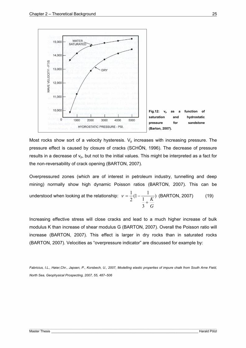
stress release, building of new joints and drying out (BARTON, 2007). vp as a function of
pressure gives “knee shaped curves” (BARTON, 2007). At very high pressures the velocity
curve for the dry state and for the saturated state are converging (Fig.12) (BARTON, 2007).
The saturated case shows the highest velocities because of the best coupling for the
fractured case (BARTON, 2007).
Chapter 2 – Theoretical Background 25
____________________________________________________________________________________________________________________________________________________________________________________________________________
Master Thesis ________________________________________________________________________________ Harald Pölzl
Fig.12: vp as a function of
saturation and hydrostatic
pressure for sandstone
(Barton, 2007).
Most rocks show sort of a velocity hysteresis. Vp increases with increasing pressure. The
pressure effect is caused by closure of cracks (SCHÖN, 1996). The decrease of pressure
results in a decrease of vp, but not to the initial values. This might be interpreted as a fact for
the non-reversability of crack opening (BARTON, 2007).
Overpressured zones (which are of interest in petroleum industry, tunnelling and deep
mining) normally show high dynamic Poisson ratios (BARTON, 2007). This can be
understood when looking at the relationship: )
3
11
1(2
1
G
K
(BARTON, 2007) (19)
Increasing effective stress will close cracks and lead to a much higher increase of bulk
modulus K than increase of shear modulus G (BARTON, 2007). Overall the Poisson ratio will
increase (BARTON, 2007). This effect is larger in dry rocks than in saturated rocks
(BARTON, 2007). Velocities as “overpressure indicator” are discussed for example by:
Fabricius, I.L., Høier,Chr., Japsen, P., Korsbech, U., 2007, Modelling elastic properties of impure chalk from South Arne Field,
North Sea, Geophysical Prospecting, 2007, 55, 487–506

Chapter 2 – Theoretical Background 26
____________________________________________________________________________________________________________________________________________________________________________________________________________
Master Thesis ________________________________________________________________________________ Harald Pölzl
2.2.6.6 Temperature
Especially low temperatures are of interest in geotechnical problems. Ice formation leads to a
20-50% velocity increase for saturated rocks compared to room temperature
(BARTON, 2007). The effect is negligible for dry rocks (BARTON, 2007). An interesting fact
is that the smallest pores freeze latest because for their less favourable area/volume ratios
(BARTON, 2007).
2.3 Correlations
This chapter should give a brief introduction and an overview on research according the
correlation between different parameters obtained in situ and/or laboratory measurements. In
a first step empirical relations for shear wave velocities from measured compressional wave
velocities are introduced. They can provide a tool for shear wave velocity estimation in areas
where no shear wave velocity could be obtained.
In a second step relations between static and dynamic moduli and between seismic
velocities and the often used unconfined compression strength are summarized. The big
advantage of geophysical in situ velocity measurements is that they offer continuous
measurement profiles and in case of good correlations to the static point measurements,
empirical relations can help in estimation of static parameters throughout larger rock or soil
volumes.

Chapter 2 – Theoretical Background 27
____________________________________________________________________________________________________________________________________________________________________________________________________________
Master Thesis ________________________________________________________________________________ Harald Pölzl
2.3.1 Velocity correlation
Many authors tried to correlate seismic wave velocities as a key to determination of lithology
from seismic or sonic logs or for seismic identification of pore fluids (MAVKO et al., 1998).
Relations are also used to predict shear wave velocity (MAVKO et al., 1998). Table 2 lists
some empirical relations out of literature.
Lithology Regression References
Sandstone 8559.08042.0, pSandstones vv [km/s] CASTAGNA, 1985, THOMSEN, 1986, CASTAGNA et al., 1993
Shale 8674.07700.0, pShales vv [km/s] CASTAGNA, 1985, THOMSEN, 1986, CASTAGNA et al., 1993
Dolomite 078.0583.0, pDolomites vv [km/s] CASTAGNA et al., 1993
Dolomite
8.1p
s
vv [km/s]
Taken from MAVKO et al., 1998 (after PICKETT, 1963*))
Limestone
9.1p
s
vv [km/s]
Taken from MAVKO et al, 1998
(after PICKETT, 1963*))
Limestone 031.1017.1055.0 2, ppLimestones vvv km/s]
CASTAGNA, 1985, THOMSEN, 1986, CASTAGNA et al., 1993
Table 2: Empirical equations for shear wave velocity from literature.
*) PICKETT., G.R., 1963. Acoustic character logs and their applications in formation evaluation: J. Can. Petr. Tech. , Vol.15, p. 659-667.
2.3.2 Static and dynamic Moduli
Moduli for the static (or very low frequency (WHITE, 1983)) case and the dynamic case show
significant differences (BARTON, 2007). The dynamic moduli are higher than the static ones
(DE VALLEJO & FERRER, 2011), reaching values of 5 to 10 times of the static ones (FJAER
et al., 1992). The difference is largest for weak rocks and decreases with increasing pressure
(FJAER et al., 1992). The biggest difference occurs for unconsolidated sediments due to
grain dislocations and consolidation processes during static load (SCHÖN, 1983). The ratio
especially rises in the near surface area (BARTON, 2007).
The differences are caused by the difference in time of stress application (tstat>>tdyn) and the
difference in particle displacements (strain) (static>>dynamic) (SCHÖN, 1983). The very
large difference of stress magnitudes between seismic or ultrasonic wave propagation and
static testing techniques is also responsible for discrepancies between static and dynamic
moduli (SCHÖN, 2011). During static deformation non-elastic components occur, whereas

Chapter 2 – Theoretical Background 28
____________________________________________________________________________________________________________________________________________________________________________________________________________
Master Thesis ________________________________________________________________________________ Harald Pölzl
ultrasonic and seismic measurements are mainly affected by the elastic response (SCHÖN,
2011). A part of the discrepancies is caused by fluid effects (FJAER et al., 1992).
Fig.13 shows the dependence of shear modulus on strain magnitude and some in situ
method examples with the typical strain levels they can achieve (LOOK, 2007).
Fig.13: Example of dependence of
shear modulus of the strain level that
can be achieved with different
methods. Dynamic geophysical
methods offer the lowest strain levels
and therefore the highest moduli
(LOOK, 2007).
Dynamic moduli also show frequency dependence, mainly influenced by the frequency
dependant mobility of fluids in the pores (CHANG et al., 2006). Generally dynamic
(compressional) moduli increase with saturation (CHANG et al., 2006). This effect is higher
at higher porosities and differs with fluid type (CHANG et al., 2006). Static Young’s Modulus
varies depending on loading/unloading path (CHANG et al, 2006). Only in dense rocks the
static moduli approach the dynamic ones (SCHÖN, 1983). With increasing porosity and
fracturing the difference between static and dynamic moduli increases (SCHÖN, 1983).
In Fig.14 and 15 the observed tendencies for relations between static and dynamic moduli of
rocks and unconsolidated materials are presented. SCHÖN, 2011 remarks that due to the
magnitude of data scatter especially for unconsolidated materials derived relations are only a
raw approximation. They must be derived in each case and for the individual rock type
(SCHÖN, 2011). SCHÖN, 2011 also mentions that the use of shear wave velocity should
result in better correlations, because shear wave velocities are controlled by the skeleton
properties of the rock and these skeleton properties predominantly control static mechanical
properties (SCHÖN, 2011).

Chapter 2 – Theoretical Background 29
____________________________________________________________________________________________________________________________________________________________________________________________________________
Master Thesis ________________________________________________________________________________ Harald Pölzl
Fig.14: Relation between static and dynamic moduli and the ratio of the moduli versus static or dynamic modulus
of rocks. The difference between static and dynamic parameters decreases from rocks with low moduli (or
velocities) to rocks with high moduli (or velocities) and from unconsolidated sediments to compact, unfractured
rocks (SCHÖN, 2011)
Fig.15: Relation between the static/dynamic
ratio and the static modulus in
unconsolidated materials (after SCHÖN,
2011).
Fig.16 shows an example for a well working correlation on a granitic rock (taken from
SCHÖN, 2011)
a
0
20
40
60
0 0.01 0.02 0.03
Crack porosity
E in
GP
a
.
E dyn
E stat
b
1
1.5
2
0 0.01 0.02 0.03
Crack porosity
E d
yn/E
sta
t
.
c
1
1.5
2
0 20 40 60
E stat in GPa
E d
yn/E
sta
t
.
d
0
20
40
60
0 20 40 60
E dyn in GPa
E s
tat
in G
Pa
.
Fig.16: Static and dynamic determined Young's modulus for
microcline-granite (figures taken from SCHÖN, 2011; after
BELIKOV et al., 1970*))
a) statE and dynE
as function of the crack porosity c ;
b) ratio statdyn EEas function of the crack porosity c ;
c) ratio statdyn EEas function of the static modulus statE
;
d) Correlation between dynE and statE
.
*) BELIKOV, B.P., ALEXANDROV, K.S., RYSOVA, T.W., 1970. Uprugie Svoistva Porodo-Obrasujscich Mineralvi Gornich Porod. Izdat. Nauka, Moskva.
Chapter 2 – Theoretical Background 30
____________________________________________________________________________________________________________________________________________________________________________________________________________
Master Thesis ________________________________________________________________________________ Harald Pölzl
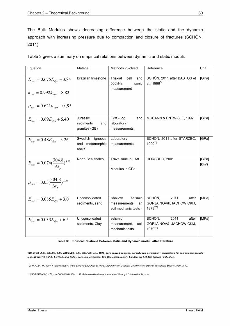
The Bulk Modulus shows decreasing difference between the static and the dynamic
approach with increasing pressure due to compaction and closure of fractures (SCHÖN,
2011).
Table 3 gives a summary on empirical relations between dynamic and static moduli:
Equation Material Methods involved Reference Unit
84.3675.0 dynstat EE
82.8992.0 dynstat kk
95.,0621.0 dynstat
Brazilian limestone Triaxial cell and
500kHz sonic
measurement
SCHÖN, 2011 after BASTOS et
al., 1998*)
[GPa]
40.669.0 dynstat EE Jurassic
sediments and
granites (GB)
FWS-Log and
laboratory
measurements
MCCANN & ENTWISLE, 1992 [GPa]
26.348.0 dynstat EE Swedish igneous
and metamorphic
rocks
Laboratory
measurements
SCHÖN, 2011 after STARZEC,
1999**)
[GPa]
23.3)8.304
(076.0p
stat tE
30.3)8.304
(03.0p
stat t
North Sea shales Travel time in µs/ft
Modulus in GPa
HORSRUD, 2001 [GPa]
[km/s]
0.3085.0 dynstat EE Unconsolidated
sediments, sand
Shallow seismic
measurements an
soil mechanic tests
SCHÖN, 2011 after
GORJAINOV&LJACHOWICKIJ,
1979***)
[MPa]
5.6033.0 dynstat EE Unconsolidated
sediments, Clay
seismic
measurement, soil
mechanic tests
SCHÖN, 2011 after
GORJAINOV& JACHOWICKIJ,
1979***)
[MPa]
Table 3: Empirical Relations between static and dynamic moduli after literature
*)BASTOS, A.C., DILLON, L.D., VASQUEZ, G.F., SOARES, J.A., 1998. Core derived acoustic, porosity and permeability correlations for computation pseudo
logs. IN: HARVEY, P.K., LOVELL, M.A. (eds.), Core-Log-Integration, 136. Geological Society, London, pp. 141-146, Special Publication.
**)STARZEC, P., 1999. Characterization of the physical properties of rocks. Department of Geology, Chalmers University of Techology, Sweden, Publ. A 90.
***)GORJANINOV, N.N., LJACHOVICKIJ, F.M., 197. Seismiceskie Metody v Insenernoi Geologii. Izdat Nedra, Moskva.

Chapter 2 – Theoretical Background 31
____________________________________________________________________________________________________________________________________________________________________________________________________________
Master Thesis ________________________________________________________________________________ Harald Pölzl
2.3.3 Unconfined compression Strength (UCS) and internal angle of friction
CHANG et al, 2006 mention UCS and internal angle of friction as key parameters for
geomechanical problems. The internal angle of friction is a measure of dependence of rock
strength on confining pressure (CHANG et al., 2006). Internal angle of friction and UCS can
be used to construct failure criteria (CHANG et al., 2006). Empirical relations can especially
be used for estimation of lower boundary of rock strength (CHANG et al., 2006). The
correlation between strength properties and seismic velocities is based on the dominant
influence of fracturing, porosity and cementation on both parameters (SCHÖN, 2011).
Increasing fracturing and/or porosity leads to a decrease of strength and seismic velocities
whereas an increase in cementation leads to an increase of both properties (SCHÖN, 2011).
Empirical relations can be used to correlate rock strength with parameters that are
measurable with geophysical well logs, especially in areas where no core material is
available (CHANG et al., 2006). Compressional wave velocity or interval transit time
(slowness), Young’s Modulus and porosity are the main geophysical log parameters used
for empirical relations (CHANG et al, 2006). Rock strength decreases with transit time and
porosity and increases with Young’s Modulus (CHANG et al., 2006). All relations need local
calibration (CHANG et al., 2006).
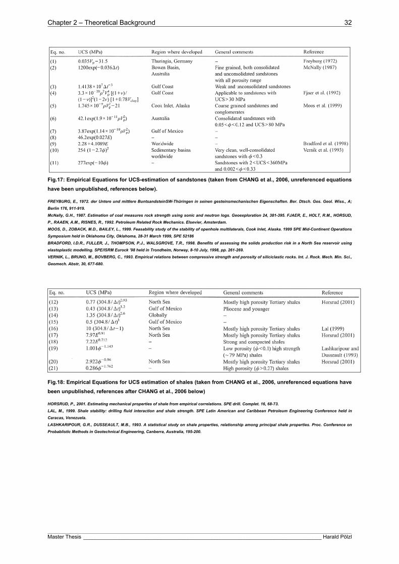
Fig.17 to 20 show different empirical equations for UCS of sandstones, shales and
limestones from different index parameters (velocities, transit time, porosity, density,…)
compiled after CHANG et al., 2006. For sandstones most of the equations underpredict the
strength at high transit times (low velocities) (CHANG et al., 2006). Porosity is not a good
strength indicator for low porosity sandstones, but a good strength indicator for shales with
high porosities (CHANG et al., 2006). In general the angle of internal friction shows an
increasing trend with vp and a decreasing trend with increasing porosity (CHANG et al.,
2006).
Chapter 2 – Theoretical Background 32
____________________________________________________________________________________________________________________________________________________________________________________________________________
Master Thesis ________________________________________________________________________________ Harald Pölzl
Fig.17: Empirical Equations for UCS-estimation of sandstones (taken from CHANG et al., 2006, unreferenced equations
have been unpublished, references below).
FREYBURG, E., 1972. der Untere und mittlere BuntsandsteinSW-Thüringen in seinen gesteinsmechanischen Eigenschaften. Ber. Dtsch. Ges. Geol. Wiss., A;
Berlin 176, 911-919.
McNally, G.H., 1987. Estimation of coal measures rock strength using sonic and neutron logs. Geoexploration 24, 381-395. FJAER, E., HOLT, R.M., HORSUD,
P., RAAEN, A.M., RISNES, R., 1992. Petroleum Related Rock Mechanics. Elsevier, Amsterdam.
MOOS, D., ZOBACK, M.D., BAILEY, L., 1999. Feasability study of the stability of openhole multilaterals, Cook Inlet, Alaska. 1999 SPE Mid-Continent Operations
Symposium held in Oklahoma City, Oklahoma, 28-31 March 1999, SPE 52186
BRADFORD, I.D.R., FULLER, J., THOMPSON, P.J., WALSGROVE, T.R., 1998. Benefits of assessing the solids production risk in a North Sea reservoir using
elastoplastic modelling. SPE/ISRM Eurock ’98 held in Trondheim, Norway, 8-10 July, 1998, pp. 261-269.
VERNIK, L., BRUNO, M., BOVBERG, C., 1993. Empirical relations between compressive strength and porosity of siliciclastic rocks. Int. J. Rock. Mech. Min. Sci.,
Geomech. Abstr, 30, 677-680.
Fig.18: Empirical Equations for UCS estimation of shales (taken from CHANG et al., 2006, unreferenced equations have
been unpublished, references after CHANG et al., 2006 below)
HORSRUD, P., 2001. Estimating mechanical properties of shale from empirical correlations. SPE drill. Complet. 16, 68-73.
LAL, M., 1999. Shale stability: drilling fluid interaction and shale strength. SPE Latin American and Caribbean Petroleum Engineering Conference held in
Caracas, Venezuela.
LASHKARIPOUR, G.R., DUSSEAULT, M.B., 1993. A statistical study on shale properties, relationship among principal shale properties. Proc. Conference on
Probablistic Methods in Geotechnical Engineering, Canberra, Australia, 195-200.

Chapter 2 – Theoretical Background 33
____________________________________________________________________________________________________________________________________________________________________________________________________________
Master Thesis ________________________________________________________________________________ Harald Pölzl
Fig.19 Empirical Equations for UCS estimation of limestones and dolomites (taken from CHANG et al., 2006,
unreferenced equations have been unpublished, references after CHANG et al., 2006 below).
MILLITZER, H., STOLL, R., 1973. Einige Beiträge der geophysics zur primadatenerfassung im Bergbau, neue Bergbautechnik, Lipzig 3, 21-25.
GOLUBEV, A.A., RABINOVICH, G.Y., 1976. Resultaty primeneia apparatury akusticeskogo karotasa dlja predeleina proconstych svoistv gornych porod na
mestorosdeniaach tverdych isjopaemych. Prikl. Geofiz. Moskva 73, 109-116.
RZHEVSKY, V., NOVICK, G., 1971. The Physics of Rocks. MIR Publ..320pp.
Fig.20: Empirical Equations for UCS estimation of siliciclastic rocks from internal
angle of friction (taken from CHANG et al., 2006, unreferenced equations have
been unpublished, references after CHANG et al., 2006 below).
LAL, M., 1999. Shale stability: drilling fluid interaction and shale strength. SPE Latin American and Caribbean Petroleum Engineering Conference held in
Caracas, Venezuela.
WEINGARTEN, J.S., PERKINS, T.K., 1995. Prediction of sand production in gas wells: methods and Gulf of Mexico case studies. J. Petrol. Tech. 596-600.

Chapter 3 –Available methods and data 34
____________________________________________________________________________________________________________________________________________________________________________________________________________
Master Thesis ________________________________________________________________________________ Harald Pölzl
3 Available methods and data
The following table (Table 4) gives an overview on the data material that was available for
this report and the methods that were used to obtain data. Descriptions of the involved
methods can be found in the appendix. Details to the sites and projects cannot be published,
due to the fact that “sensitive” projects (nuclear power plants for example) are involved and
due to the fact that some projects are still in progress.
Country Project Dominant lithology Stat. lab Stat. in situ Dyn. lab Dyn. in situ
USA NPP
Shaly limestones
Sandstones
Shale
Unconsoloditated sediments
3-AX
1-AX - USP shear wave only
SASW/MASW
PSSL
DH
Austria Express Highway
Granites
(Grano)Diorites
Aplites
Pegmatites
3-AX
1-AX DIL - FWS+GGD
Austria Tunnel Metamorphic rocks (mainly gneisses)
3-AX
1-AX - - FWS+GGD
Hong Kong
Seismic Microzonation
Metasediments
Vulcanoclastics
Unconsolidated sediments
- - -
PSSL
CH
DH
UK NPP Metasediments
Microgabbro
3-AX
1-AX DIL
USP compressional and shear wave
PSSL
Dubai Infrastructure Sedimentary rocks
Sands 1-AX - - CH
Quatar Infrastructure Sedimentary Rocks 1-ax - - PSSL
Table 4: Overview on sites, dominant lithologies and methods that were available fort his report.
Abbreviations:
NPP Nuclear Power Plant
3-AX 3-axial tests
1-AX Unconfined Compression Tests
DIL Dilatometer tests
SASW/MASW (Multichannel) Analysis of surface waves
PSSL PS Suspension Logging
FWS+GGD Full waveform sonic logging with Gamma-Gamma density logging
DH Downhole seismics
CH Crosshole seismics
USP Ultrasonic pulse velocity measurements

Chapter 4 – Comparison of different dynamic methods 35
____________________________________________________________________________________________________________________________________________________________________________________________________________
Master Thesis ________________________________________________________________________________ Harald Pölzl
4 Comparison of different dynamic methods
Before analysing relationships between static and dynamic methods, a closer look on the
dynamic methods for velocity measurements is performed. In this chapter velocities from
different available methods are directly compared. A similar comparison for the static
methods was unfortunately not possible, because of lacking “data intersection”.
Directly means that it was tried to compare only velocity values that were measured in the
same borehole and the same depth (except the velocities obtained with Multichannel
Analysis of Surface Waves - MASW). MASW velocities have been compared with velocity
values measured with other methods in boreholes as close as possible to the MASW profiles
(several meters to several tens of meters away from the MASW profiles).
Fig.21 shows a direct comparison of shear wave velocity measurements with MASW, PS
Suspension Logger (PSSL) and downhole seismic measurements in a succession of (shaly)
limestones, shales and (shaly) sandstones in the US. Downhole seismics and PSSL have
been measured in the same boreholes (BH-1 in Fig.21 left and BH-2 Fig.21 right). MASW
measurements were performed very close to the boreholes. The log shows that MASW and
PSSL are correlating rather well for both boreholes. The differences between these two
methods are mainly caused by the higher vertical resolution of PSSL, which allows displaying
smaller scale velocity variations that are not resolved by MASW. A point that must also be
taken into account is the difference in measurement frequencies. MASW uses frequencies in
the range of a few to a few tens of Hz, whereas PSSL uses frequencies in the range of 0.5 to
5 kHz.
Compared to these two methods, the downhole measurements offer rather ambivalent
results. In some areas the downhole velocities correlate very well with the velocities
measured with the two other methods, but there are more sections were downhole velocities
are far away from the velocities measured with the other two methods. Reason for that might
be that the increasing source receiver offset of the downhole measurement leads to
increasing attenuation of (especially) higher frequencies in the increasing investigated rock
or soil volume. This loss of the higher frequencies increases difficulties in first arrival picking,
especially for the shear wave.

Chapter 4 – Comparison of different dynamic methods 36
____________________________________________________________________________________________________________________________________________________________________________________________________________
Master Thesis ________________________________________________________________________________ Harald Pölzl
Fig.21: Direct comparison of shear wave velocity measurements with PSSL, MASW and downhole seismics. MASW and
PSSL velocities show good correlation. Differences are mainly based on different vertical resolutions (PSSL>MASW)
and different measurement frequencies (PSSL>MASW). Downhole velocities show good correlation in some sections
and rather bad or no correlation in other sections.
Fig.22 shows a similar plot for direct comparison of vp from downhole seismic and PSSL and
vs from crosshole seismic, PSSL and downhole measurements in a metamudstone formation
in Hong Kong overlain by a few meters of unconsolidated silty sediments. Crosshole
measurements have been performed with “splitted” shear waves, meaning that a source has
been used, that is capable of activating horizontal propagating, vertical polarized (vs,hv) and
horizontal propagating, horizontal polarized (vs,hh) shear waves. The comparison of vp (left
log) shows a large difference between PSSL and downhole measurements (up to 500 m/s).
This might be caused by a combination of a frequency effect, (larger scale) fracturing of the
formation and alteration of the borehole wall. Of course the already mentioned effect of high
frequency energy loss might play a role too. Shear wave velocity comparison shows that the
three methods correlate well up to a depth of about 17.0 m. Beyond this depth PSSL (where
available) and crosshole follow a similar shear wave velocity trend, whereas downhole
velocities show an increasing difference to the other two methods. The shear wave profile
derived from downhole measurements shows rather constant vs, which seems to be
unreliable for the deeper regions of the borehole.

Chapter 4 – Comparison of different dynamic methods 37
____________________________________________________________________________________________________________________________________________________________________________________________________________
Master Thesis ________________________________________________________________________________ Harald Pölzl
Fig.22: Direct
comparison of vp from
downhole and PSSL-
measurements (LEFT)
and vs from downhole,
PSSL and splitted
shear wave crosshole
measurements.
In Fig.23 the shear wave velocities from the same data set as in Fig.22 measured with
crosshole and PSSL are compared in a velocity crossplot. Generally the velocities show very
good correlation and seem to fit to a linear trend. A small population of PSSL velocities
shows slightly lower velocity values than the crosshole velocities. This might be interpreted
as result of borehole sections with significant wall alteration, which does not really affect
crosshole velocities, but has a significant influence on PSSL measurements. Another
explanation might be that the difference between the horizontal propagating waves used for
crosshole measurements and the vertical propagating waves of PSSL are caused by
anisotropic behaviour of the material.

Chapter 4 – Comparison of different dynamic methods 38
____________________________________________________________________________________________________________________________________________________________________________________________________________
Master Thesis ________________________________________________________________________________ Harald Pölzl
0
200
400
600
800
1000
0 200 400 600 800 1000
Crosshole velocity [m/s]
PS
SL
vel
oci
ty [
m/s
]
vs,hh
vs,hv
Fig.23: Velocity crossplot to compare shear wave velocities measured with PSSL and crosshole
measurements (dual measurements with horizontal and vertical polarized and horizontal propagating
shear waves). Generally a good correlation can be observed. A small population of PSSL velocities
shows slight deviation from the line of direct proportionality, maybe caused by a higher borehole wall
alteration or anisotropy.
The dual crosshole measurements using horizontal propagating shear waves with vertical
(vs,hv) and horizontal (vs,hh) polarization (shear wave splitting) can also be used to estimate
velocity anisotropy of the formation(Fig.24), as already indicated by the comparison of
crosshole and PSSL measurements. The crossplot of the two shear wave velocities
(Fig.24 TOP) already suggests slight anisotropy. A calculated trend line leads to increasing
anisotropy with increasing shear wave velocity. Plotting the velocity ratio against the shear
wave velocity shows the anisotropic behaviour of the encountered formations a bit better.
The velocity ratio reaches values up to 1.6.

Chapter 4 – Comparison of different dynamic methods 39
____________________________________________________________________________________________________________________________________________________________________________________________________________
Master Thesis ________________________________________________________________________________ Harald Pölzl
0
500
1000
1500
2000
0 500 1000 1500 2000
vs,hh [m/s]
v s,h
v [
m/s
]
Crosshole Data
Line of Isotropy
exponential fit to data
0
0,5
1
1,5
2
0 500 1000 1500 2000
vs [m/s]
v s,h
h/v
s,h
v [m
/s]
vs,hh
vs,hv
Fig.24: TOP: Velocity of a horizontal propagating, vertical polarized shear wave (vs,hv) as a function of the
velocity of a horizontal propagating and horizontal polarized shear wave (vs,hh) derived from crosshole seismic
data. The exponential fit to the data suggests an increasing anisotropy with increasing velocity.
BOTTOM: Crossplot of shear wave velocity (vs,hh and vs,hv versus vs,hh/ vs,hv-ratio indicating a significant effect
of shear wave splitting, which can be interpreted as sign of formation velocity anisotropy.

Chapter 4 – Comparison of different dynamic methods 40
____________________________________________________________________________________________________________________________________________________________________________________________________________
Master Thesis ________________________________________________________________________________ Harald Pölzl
In Fig.25 downhole measurements and PSSL measurements in two formations are
compared. The downhole measurements show very low wave velocities of doubtful reliability.
The PSSL measurements offer more scattering data, but the velocities are higher and are
therefore seen to be more reliable than the downhole velocities. A small amount of the
difference might be caused by a frequency effect. The main problem here might be that first
arrival picking on downhole data in highly attenuating formations is very difficult and can lead
to mispicks. The PSSL method (or also FWS) with a low and constant source receiver offset
should be preferred (if possible).
0
500
1000
1500
2000
0 1000 2000 3000 4000
vp [m/s]
v s [m
/s]
Granites, downhole
Metaconglomerate, downhole
Granites, PSSL
Metaconglomerate, PSSL
Fig.25: vp-vscrossplot for downhole and PSSL velocities, measured in the same depths in the same metaconglomerate
and granite formation, but not in the same borehole. Downhole velocities for both lithologies show a good linear trend
but compared to the PSSL velocities they are significantly lower.
Fig.26 shows direct comparison between PSSL and downhole velocity measurements in a
succession of (shaly) limestones, shales and (shaly) sandstones. Except a population of data
points with deviating high downhole velocities, which cannot be reasoned for sure; the two
methods offer moderate to good correlating compressional and shear wave velocities.

Chapter 4 – Comparison of different dynamic methods 41
____________________________________________________________________________________________________________________________________________________________________________________________________________
Master Thesis ________________________________________________________________________________ Harald Pölzl
0
5000
10000
15000
20000
25000
30000
0 5000 10000 15000 20000 25000 30000
PSSL velocity [ft/s]
Do
wn
ho
le v
elo
city
[ft
/s]
Compressional w ave
Shear w ave
Fig.26: Direct comparison of downhole and PSSL measurements in a succession of (shaly)
limestones, shales and (shaly (sandstones). Except the marked data point population the
correlation is good to moderate.
A comparison of velocities from laboratory and PSSL measurements is shown in Fig.27 and
Fig.28. The two methods show generally good correlation for compressional and shear wave
velocity. Laboratory velocities seem to be slightly higher, what might be mainly a result of the
higher measurement frequencies in laboratory and the use of compact samples without
fractures in case of laboratory specimens. In Fig.27 two outliers can be observed in the high
laboratory velocity region >12500 ft/s. This might be caused by measurements on a very
clean and rather unaltered limestone sample or the compressional wave velocities of the
samples have been measured.
?

Chapter 4 – Comparison of different dynamic methods 42
____________________________________________________________________________________________________________________________________________________________________________________________________________
Master Thesis ________________________________________________________________________________ Harald Pölzl
0
2500
5000
7500
10000
12500
15000
0 2500 5000 7500 10000 12500 15000
vs, Lab [ft/s]
v s,
PS
SL [
ft/s
]
Limestone
Sandstone
Shale
Fig.27: Comparison of
shear wave velocity
from laboratory trans-
mission measure-
ments and PSSL,
showing good to
moderate correlation.
The extreme outliers on
the right plot side
might be a result of
shear wave velocity
measurements in very
clean and unaltered
limestone samples of
the site or instead of
shear wave velocity
compressional wave
velocity was measured.
1000
2000
3000
4000
5000
6000
7000
1000 2000 3000 4000 5000 6000 7000
vlab [m/s]
vP
SS
L [
m/s
]
compressional wave
shear wave
Fig.28: Comparison of
shear wave velocities
measured with PSSL
and data from
laboratory in a
metasediment dom-
inated lithology
providing a moderate
to good correlation.
Velocities from lab are
higher than the PSSL
velocities. The
difference is seen to be
caused mainly by the
higher frequencies
used in the laboratory
measurements.
4.1 Conclusions
Under the assumption of “correct” measurement procedure and data interpretation
(especially no widespread first arrival mispicking and no significant depth differences
between the compared measurements)) the different dynamic methods for acoustic velocity
determination of rocks and soils should offer well to moderately correlating velocity values.
Differences between methods are mainly caused by frequency and scale effects. Especially

Chapter 4 – Comparison of different dynamic methods 43
____________________________________________________________________________________________________________________________________________________________________________________________________________
Master Thesis ________________________________________________________________________________ Harald Pölzl
for the comparison of laboratory velocities to in situ velocities it has to be taken into account
that laboratory measurements use relative high frequencies on very small and usually intact
samples, whereas in situ measurements use at least slightly lower frequencies and are
affected by discontinuities like fractures or faults and use lower frequencies than the
laboratory techniques.
Differences in the vertical resolution of the compared methods can also cause local
differences between velocities (for example between MASW and PSSL). Although the
general velocity trend is the same in the different measurements, the higher resolving
method shows locally small scale velocity changes, which are averaged by the method with
the lower resolution.
Compared to the other methods the downhole method seems to be the most “problematic”.
Results can be ambiguous, meaning that the downhole method offers good correlating
velocity values in some sections and not correlating values in other sections of a borehole.
The biggest problem in the author’s opinion is that the source receiver offset is increasing
during measurements. The source usually remains at the surface, whereas the receiver is
lowered in the borehole. The increasing rock and/or soil volume during measurement leads
to increasing attenuation, especially of higher frequencies, what can lead to difficulties in
correct first arrival determination. Therefore the downhole method should only be performed
where other methods (with constant source and receiver offset like full waveform sonic log
for example) cannot be applied (dry holes or unstable holes that require PVC casing for
example).
5 Relations between vp and vs
The vp/vs-ratio is an important property for seismic applications. In order to estimate shear-
wave velocities when only compressional wave velocities are available,
CASTAGNA et al.,1985 derived an empirical equation commonly referred to as the
“mudrock-line” (mudrock: “clastic silicate rock composed primarily of clay or silt sized
particles”):
1724.18621.0 ps VV [km/s] (20)
Numerous researchers have published variants of the mudrock equation (SCHÖN, 2011)
According to the principle of the mudrock equation relations between compressional wave
velocities (vp) and shear wave velocities (vs) for different lithologies and different methods are

Chapter 5 – Correlations between vp and vs 44
____________________________________________________________________________________________________________________________________________________________________________________________________________
Master Thesis ________________________________________________________________________________ Harald Pölzl
analysed in this chapter. Target is to derive reliable empirical relations for vs from measured
vp. In geotechnical applications this could help in estimation of vs in areas where it was
possible to measure vp, but not vs. The relations in this chapter are mainly linear regressions,
calculated with MS Excel. The statistical error parameter is the R² value, which is
automatically calculated by MS Excel.
In a first step a global analysis was tried. Fig.29 shows a vp-vs cross plot for the average
velocities (including standard deviation bars) from the different available datasets
differentiating different lithologies and methods. The standard deviation lies usually beyond
or around 5%. An exception with standard deviations exceeding 20% are downhole velocities
measured in a layered shale and shaly limestone succession in the intermediate velocity
range. The average velocities follow a surprisingly good linear trend (R²=0.92).
0
500
1000
1500
2000
2500
3000
3500
4000
0 1000 2000 3000 4000 5000 6000 7000
vp [m/s]
v s[m
/s]
shaly limestone-PSSL
shaly sandstone-PSSL
shale-PSSL
Unconsolidated Sediments-PSSL
Limestone-DH
limestone dominated-DH
shale dominated-DH
Aplite-FWS
Diorite A-FWS
Granite A-FWS
Granodiorite A-FWS
Pematite A-FWS
Granite B-FWS
Granodiorite B-FWS
Granite C-FWS
Pegmatite B-FWS
Unconsolidated Seds B-PSSL
Metased.-PSSL
Microgabbro-PSSL
Metased.-LAB
Calcsiltite-CH
Siltstone-PSSL
Sand-CH
Fig.29: vp-vs crossplot for the different methods and lithologies encountered in the data for his report. A rough
differentiation of the different lithologies is possible as pointed out in the plot. The intermediate velocity range is only
covered by a layered shale limestone succession measured with downhole seismics, showing rather large standard
deviations (up to 20%). For the other datasets standard deviations lie around 5%. The resulting velocity distribution
can be approximated with a linear regression of rather good fit: 17.3945901.0 ps vv with R²=0.92. Rather high
standard deviations occur, because all measurements are performed in the first 100 m below the surface (lithological
inhomogeneities, influence of weathering, different saturation degrees, …).
Magmatic
and metamorphic
Uncons. and
low grade cons.
sediments
Consolidated
sediments and
sedimentary
rocks

Chapter 5 – Correlations between vp and vs 45
____________________________________________________________________________________________________________________________________________________________________________________________________________
Master Thesis ________________________________________________________________________________ Harald Pölzl
In a next step the vp-vs-relations for the different sites and methods were analyzed separately
to derive and evaluate empirical relations for each site. Table 5 shows a summary of the
found relations sorted by their R² value (from highest to lowest).
Relation R² Lithology Location Method Comment Unit
0439.05216.0 ps vv 0.98 Siltstones/Calcsiltites Dubai CH No differentiation
of lithologies [km/s]
pvs ev 125390977.0 0.90 Sands*) Dubai CH
Variable degree of
cementation [km/s]
95.4374677.0 ps vv 0.84 Granites Austria FWS Very shallow,
zmax=30 m [m/s]
1151.05511.0 ps vv 0.80 Sands*) Dubai CH Variable degree of
cementation [km/s]
1.14356173.0 ps vv 0.77 Limestones US PSSL Significant shale
content [ft/s]
18.1345124.0 ps vv 0.74 Granites Austria FWS zmax=110 m [m/s]
05.1113822.0 ps vv 0.72 Unconsolidated Sediments US PSSL
No “acoustic”
differentiaton of
different lithologies
according to their
velocity.
[ft/s]
36.3546031.0 ps vv 0.64 Metasediments UK PSSL - [m/s]
52.695527.0 ps vv 0.61 Sandstones US PSSL Shaly [ft/s]
298.424843.0 ps vv 0.60 Granodiorites Austria FWS Very shallow,
zmax=30 m [m/s]
31.540474.0 ps vv 0.57 Shale US PSSL - [ft/s]
03.7623458.0 ps vv 0.29 Microgabbro UK PSSL Low number of
data values [m/s]
65.980363.0 ps vv 0.23 Plutonic rocks Austria FWS
No “acoustic”
differentiation
between granites,
granodiorites and
diorites, zmax=80 m
[m/s]
9.22741261.0 ps vv 0.15 Shaly limestones,
sandstones and shale US DH - [ft/s]
24.1782735.0 ps vv 0.09 Unconsolidated Sediments Hong Kong PSSL
No seismic
differentiation
between clay, silt
and sand
[m/s]
Table 5: Empirical relations for different sites and lithologies sorted after their R² value.
*) Same sands but different regression type. The exponential approach offered slightly better fit to the data than the linear
approach.
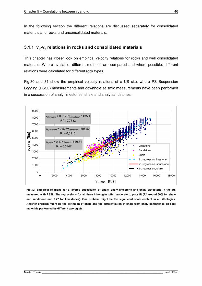
Chapter 5 – Correlations between vp and vs 46
____________________________________________________________________________________________________________________________________________________________________________________________________________
Master Thesis ________________________________________________________________________________ Harald Pölzl
In the following section the different relations are discussed separately for consolidated
materials and rocks and unconsolidated materials.
5.1.1 vp-vs relations in rocks and consolidated materials
This chapter has closer look on empirical velocity relations for rocks and well consolidated
materials. Where available, different methods are compared and where possible, different
relations were calculated for different rock types.
Fig.30 and 31 show the empirical velocity relations of a US site, where PS Suspension
Logging (PSSL) measurements and downhole seismic measurements have been performed
in a succession of shaly limestones, shale and shaly sandstones.
vs,limestone = 0.6173vp,limestone - 1435.1
R2 = 0.7732
vs,sandstone = 0.527vp,sandstone - 695.52
R2 = 0,6115
vs,shale = 0.474vp,shale - 540.31
R2 = 0.5747
0
1000
2000
3000
4000
5000
6000
7000
8000
9000
0 2000 4000 6000 8000 10000 12000 14000 16000 18000
vp, PSSL [ft/s]
vs
,PS
SL [
ft/s
]
Limestone
Sandstone
Shale
lin. regression limestone
lin. regression, sandstone
lin. regression, shale
Fig.30: Empirical relations for a layered succession of shale, shaly limestone and shaly sandstone in the US
measured with PSSL. The regressions for all three lithologies offer moderate to poor fit (R² around 60% for shale
and sandstone and 0.77 for limestones). One problem might be the significant shale content in all lithologies.
Another problem might be the definition of shale and the differentiation of shale from shaly sandstones on core
materials performed by different geologists.
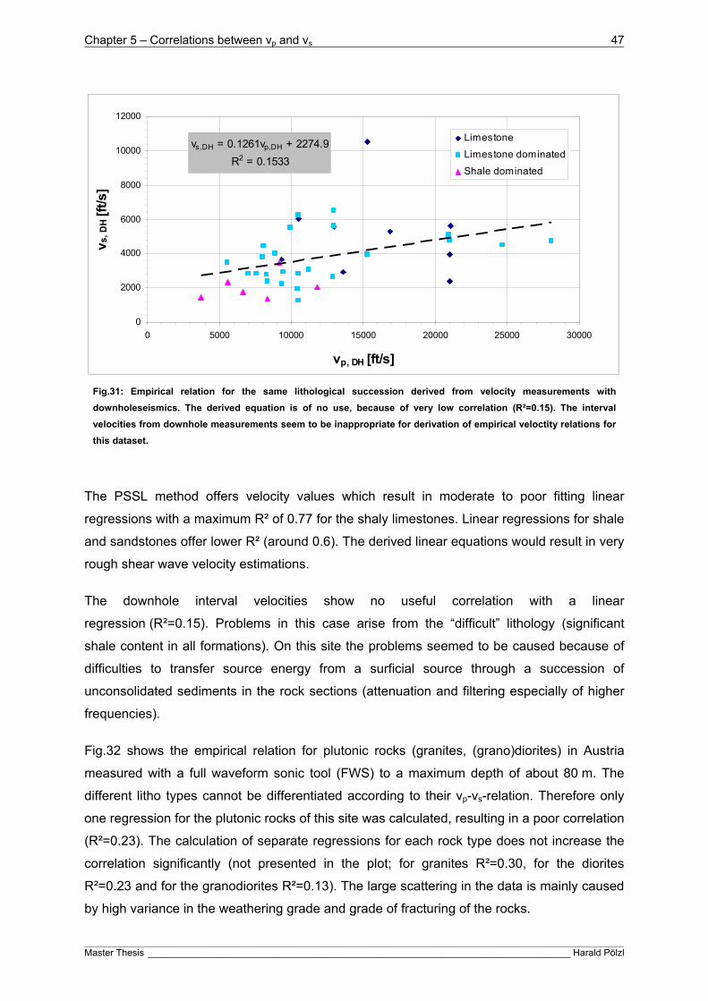
Chapter 5 – Correlations between vp and vs 47
____________________________________________________________________________________________________________________________________________________________________________________________________________
Master Thesis ________________________________________________________________________________ Harald Pölzl
vs,DH = 0.1261vp,DH + 2274.9
R2 = 0.1533
0
2000
4000
6000
8000
10000
12000
0 5000 10000 15000 20000 25000 30000
vp, DH [ft/s]
vs,
DH [
ft/s
]
Limestone
Limestone dominated
Shale dominated
Fig.31: Empirical relation for the same lithological succession derived from velocity measurements with
downholeseismics. The derived equation is of no use, because of very low correlation (R²=0.15). The interval
velocities from downhole measurements seem to be inappropriate for derivation of empirical veloctity relations for
this dataset.
The PSSL method offers velocity values which result in moderate to poor fitting linear
regressions with a maximum R² of 0.77 for the shaly limestones. Linear regressions for shale
and sandstones offer lower R² (around 0.6). The derived linear equations would result in very
rough shear wave velocity estimations.
The downhole interval velocities show no useful correlation with a linear
regression (R²=0.15). Problems in this case arise from the “difficult” lithology (significant
shale content in all formations). On this site the problems seemed to be caused because of
difficulties to transfer source energy from a surficial source through a succession of
unconsolidated sediments in the rock sections (attenuation and filtering especially of higher
frequencies).
Fig.32 shows the empirical relation for plutonic rocks (granites, (grano)diorites) in Austria
measured with a full waveform sonic tool (FWS) to a maximum depth of about 80 m. The
different litho types cannot be differentiated according to their vp-vs-relation. Therefore only
one regression for the plutonic rocks of this site was calculated, resulting in a poor correlation
(R²=0.23). The calculation of separate regressions for each rock type does not increase the
correlation significantly (not presented in the plot; for granites R²=0.30, for the diorites
R²=0.23 and for the granodiorites R²=0.13). The large scattering in the data is mainly caused
by high variance in the weathering grade and grade of fracturing of the rocks.
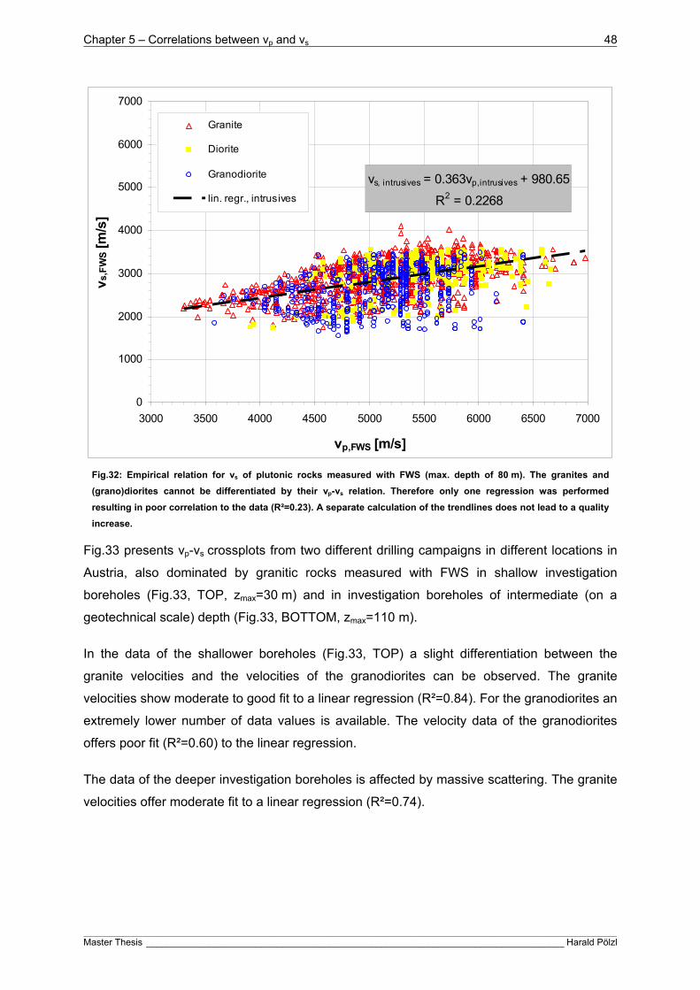
Chapter 5 – Correlations between vp and vs 48
____________________________________________________________________________________________________________________________________________________________________________________________________________
Master Thesis ________________________________________________________________________________ Harald Pölzl
vs, intrusives = 0.363vp,intrusives + 980.65
R2 = 0.2268
0
1000
2000
3000
4000
5000
6000
7000
3000 3500 4000 4500 5000 5500 6000 6500 7000
vp,FWS [m/s]
vs,
FW
S [
m/s
]
Granite
Diorite
Granodiorite
lin. regr., intrusives
Fig.32: Empirical relation for vs of plutonic rocks measured with FWS (max. depth of 80 m). The granites and
(grano)diorites cannot be differentiated by their vp-vs relation. Therefore only one regression was performed
resulting in poor correlation to the data (R²=0.23). A separate calculation of the trendlines does not lead to a quality
increase.
Fig.33 presents vp-vs crossplots from two different drilling campaigns in different locations in
Austria, also dominated by granitic rocks measured with FWS in shallow investigation
boreholes (Fig.33, TOP, zmax=30 m) and in investigation boreholes of intermediate (on a
geotechnical scale) depth (Fig.33, BOTTOM, zmax=110 m).
In the data of the shallower boreholes (Fig.33, TOP) a slight differentiation between the
granite velocities and the velocities of the granodiorites can be observed. The granite
velocities show moderate to good fit to a linear regression (R²=0.84). For the granodiorites an
extremely lower number of data values is available. The velocity data of the granodiorites
offers poor fit (R²=0.60) to the linear regression.
The data of the deeper investigation boreholes is affected by massive scattering. The granite
velocities offer moderate fit to a linear regression (R²=0.74).

Chapter 5 – Correlations between vp and vs 49
____________________________________________________________________________________________________________________________________________________________________________________________________________
Master Thesis ________________________________________________________________________________ Harald Pölzl
vs,granites= 0.4677vp,granites + 437.95
R2 = 0.836
vs,granodiorites = 0.4843vp,granodiorites + 42.298
R2 = 0.5979
0
500
1000
1500
2000
2500
3000
3500
4000
2000 2500 3000 3500 4000 4500 5000 5500 6000 6500 7000
vp,FWS [m/s]
vs,
FW
S [
m/s
]
Granite
Granodiorite
Linear (Granite)
Linear (Granodiorite)
vs,granite = 0.5124vp,granite + 134.18
R2 = 0.74
0
1000
2000
3000
4000
2000 3000 4000 5000 6000 7000
vp,FWS [m/s]
vs,
FW
S [
m/s
]
Granite
lin. regression, granite
Fig.33: Velocity crossplot for FWS measurements in shallow investigation boreholes with zmax around 30 m (TOP) and
investigation boreholes of intermediate depth (zmax around 110 m) in a mainly granitic environment offering moderate
fitting linear trends for granites and poor fitting linear trend for granodiorites.
In Fig.34 the results of crosshole velocity measurements in a calcsiltite-siltstone succession
in the Dubai are shown in a velocity crossplot. The different lithologies cannot be clearly
differentiated from each other according to their velocities. A high velocity region
(>2.250 km/s) for siltstones can be defined. No further differentiation is possible. For this

Chapter 5 – Correlations between vp and vs 50
____________________________________________________________________________________________________________________________________________________________________________________________________________
Master Thesis ________________________________________________________________________________ Harald Pölzl
reason only 1 regression was calculated resulting in a very good fit (R²=0.98) to the data.
The derived equation seems to be reliable and appropriate enough to be used for shear
wave velocity estimations on this site.
vs = 0.5216vp - 0.0439
R2 = 0.9779
0.00
0.50
1.00
1.50
2.00
0.00 0.50 1.00 1.50 2.00 2.50 3.00 3.50 4.00
vp,CH [km/s]
vs,
CH [
km
/s]
Calcsiltite
Siltstone
Calcsiltite/Siltstone
lin. regression
Fig.34: Velocity crossplot for crosshole seismic measurements in a siltstone-calcsiltite
succession and a very good fitting linear regression to the data, suitable for appropriate shear
wave estimations from vp.
Fig.35 shows the results of PSSL measurements in a metasediment
succession (metaconglomerate, mud- and –siltstone) and a microgabbro encountered by
nearshore investigation boreholes in the UK area. The velocities in the metasediments cover
a relative wide range and are affected by scattering. The derived linear equation shows poor
fit to the data (R²=0.64). The microgabbros show compressional wave velocities larger than
5000 m/s. A relative low number of available data points and relative massive data scatter
lead to a linear regression with no significant fit to the data.
vs,metasediments = 0.6031vp, metasediments - 354.36
R2 = 0.6435
vs,microgabbro = 0.3458vp,microgabbro + 762.03
R2 = 0.28640
500
1000
1500
2000
2500
3000
3500
4000
3000 3500 4000 4500 5000 5500 6000 6500
vp,PSSL [m/s]
vs,
PS
SL [
m/s
]
Metasediments
Microgabbro
lin. regression, metasediments
lin. regression, microgabbro
Fig.35: Velocity
crossplot for PSSL-
measurements in
metasediments and
gabbros resulting in
moderate to poor
fitting linear
regressions for vs.
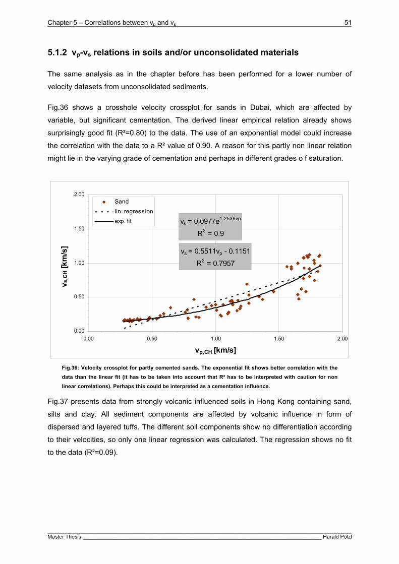
Chapter 5 – Correlations between vp and vs 51
____________________________________________________________________________________________________________________________________________________________________________________________________________
Master Thesis ________________________________________________________________________________ Harald Pölzl
5.1.2 vp-vs relations in soils and/or unconsolidated materials
The same analysis as in the chapter before has been performed for a lower number of
velocity datasets from unconsolidated sediments.
Fig.36 shows a crosshole velocity crossplot for sands in Dubai, which are affected by
variable, but significant cementation. The derived linear empirical relation already shows
surprisingly good fit (R²=0.80) to the data. The use of an exponential model could increase
the correlation with the data to a R² value of 0.90. A reason for this partly non linear relation
might lie in the varying grade of cementation and perhaps in different grades o f saturation.
vs = 0.5511vp - 0.1151
R2 = 0.7957
vs = 0.0977e1.2539vp
R2 = 0.9
0.00
0.50
1.00
1.50
2.00
0.00 0.50 1.00 1.50 2.00
vp,CH [km/s]
vs,
CH [
km
/s]
Sand
lin. regression
exp. fit
Fig.36: Velocity crossplot for partly cemented sands. The exponential fit shows better correlation with the
data than the linear fit (it has to be taken into account that R² has to be interpreted with caution for non
linear correlations). Perhaps this could be interpreted as a cementation influence.
Fig.37 presents data from strongly volcanic influenced soils in Hong Kong containing sand,
silts and clay. All sediment components are affected by volcanic influence in form of
dispersed and layered tuffs. The different soil components show no differentiation according
to their velocities, so only one linear regression was calculated. The regression shows no fit
to the data (R²=0.09).

Chapter 5 – Correlations between vp and vs 52
____________________________________________________________________________________________________________________________________________________________________________________________________________
Master Thesis ________________________________________________________________________________ Harald Pölzl
vs,unconsolitated = 0.2735vp,unconsolitated - 178.24
R2 = 0.0904
0
200
400
600
800
1000
1000 1300 1600 1900 2200 2500vp,PSSL [m/s]
vs,
PS
SL [
m/s
]Clay
Sand
Silt
lin. regression
Fig.37: vp-vs crossplot for soils influenced by dispersed and layered tuffs. The data shows no
significant fit to a linear regression.
Fig.38 shows a velocity crossplot for unconsolidated materials (residual soil, artificial fill, silt
and clay and weathered limestone) measured with PSSL in a sediment succession in the
US. The derived linear regression (only one because of lacking differentiation of different
lithologies) offers moderate fit to the data (R²=0.72).
vs,uncons. = 0.3822vp,uncons. + 111.05
R2 = 0.7211
0
1000
2000
3000
4000
5000
0 1000 2000 3000 4000 5000 6000 7000 8000
vp,PSSL [ft/s]
vs,
PS
SL [
ft/s
]
Clay
w eathered Limestone
RS/AF
Silt
Fig.38: Velocity crossplot for different unconsolidated materials measured with PSSL. The linear regression
shows moderate fit to the data.

Chapter 5 – Correlations between vp and vs 53
____________________________________________________________________________________________________________________________________________________________________________________________________________
Master Thesis ________________________________________________________________________________ Harald Pölzl
5.1.3 Conclusions
The use of empirical relations to derive vs from measured vp for rocks as well as for
unconsolidated materials is limited by rather moderate fit of the scattering data to a linear
regression. Only rough estimations of vs are possible. At this point it may be noted that from
a physics point of view there is no strong correlation between the two parameters, because
the elastic behaviour is controlled by the independent properties for compression and shear.
Empirical regressions therefore can reflect only a tendency originated by similar influence of
mineral composition, fracturing etc. on the two velocities.
It seems that crosshole seismic measurements offer the highest data quality for derivation of
empirical relations (in rocks and soils). All empirical relations derived from crosshole
measurements offered good to excellent fit (R²>0.80) to the data.
On the other end of the scale downhole measurements and PSSL measurements in
unconsolidated materials seem to offer velocity data that cannot be used for the derivation of
empirical relations. In the presented datasets another problem occurs. The differentiation of
similar lithologies by several geologists is not always distinct and this causes problems for
rock specific empirical equations.
Another problem in deriving rock specific empirical relations might be the non uniqueness of
lithology classification. The same material might be classified in a different way by different
geologists. For example the distinction between shale and mud- or siltstones or the
distinction between different granitic rocks might not always be that clear.

Chapter 6 – Correlations between static and dynamic moduli 54
____________________________________________________________________________________________________________________________________________________________________________________________________________
Master Thesis ________________________________________________________________________________ Harald Pölzl
6 Correlations between static and dynamic moduli
In this chapter the available data sets are analyzed for correlations between the calculated
dynamic elastic moduli and measured or calculated static moduli. Although a large amount of
data was available for different methods only a few intersections were found, where direct
correlations (same borehole same depth and data of a dynamic and a static measurement)
were possible. It was tried to find linear relationships for the correlation between static
modulus and dynamic modulus according to the ones found in literature and mentioned in
chapter 2.3.2:
baEE dynstat (21)
where a and b are empirically.
On the other hand it was tried to derive power law relations from the crossplots of static
modulus versus the dynamic/static ratio to improve correlations with the same number of free
parameters:
ddynstat c
EE )(
(22)
where c and d are empirically.
The first example presented in Fig.39 - 41 shows the comparison and correlation of dynamic
modulus from crosshole seismic testing and static modulus from unconfined compression
strength tests for a succession of siltstones and calcarenites in Dubai. The calculated
relations with
422005.0 dynstat EE (23)
84.01234 statstat
dyn EE
E
(24)
or solved for static modulus
3.6)1234
( dynstat
EE ) (25)
show no fit to the data (Fig.39 and Fig.40). The direct comparison of the static and dynamic
moduli shows that the dynamic moduli are much higher than the static ones. The calculated
regression offers no fit to the data (R²=0) and shows a very low gradient (nearly approaching

Chapter 6 – Correlations between static and dynamic moduli 55
____________________________________________________________________________________________________________________________________________________________________________________________________________
Master Thesis ________________________________________________________________________________ Harald Pölzl
constant static modulus). Using the relation between the dynamic/static-ratio and the static
modulus raises R² to 0.31, which is much better than the former approach, but still no
significant fit to the data is given.
Estat = 0.0047Edyn + 421.6
R2 = 0.0036
0
1000
2000
3000
4000
5000
0 5000 10000 15000
Edyn,CH [MPa]
Est
at,U
CS [
MP
a]
CH distance 3m
CH distance 6m
lin. regression
Fig.39: direct comparison
between Edyn and Estat from
crosshole seismics and
UCS-tests. The dynamic
moduli are much higher
than the static ones. The
resulting linear regression
shows a very low gradient
and no significant fit to the
data.
Edyn/Estat = 1234.3Estat-0.8415
R2 = 0.3086
1
10
100
1000
1 10 100 1000 10000
Estat, UCS [MPa]
Ed
yn,C
H/E
stat
,UC
S [
1]
CH distance 3m
CH distance 6m
Power Law Relation
Fig.40: dynamic/static
ratio as a function of Estat.
The ratio goes up to
values of about 100. A
calculated power law
relation shows higher fit
than the linear one but
with R²=0.31 it still shows
no significant fit to the
data.
The only result that can be assumed by an empirical relation seems to be the maximum
dyn./stat.-ratio (Fig.41) on the linear plot of the ratio as a function of static modulus.
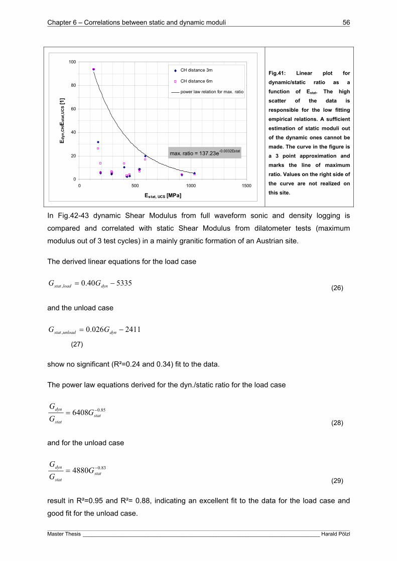
Chapter 6 – Correlations between static and dynamic moduli 56
____________________________________________________________________________________________________________________________________________________________________________________________________________
Master Thesis ________________________________________________________________________________ Harald Pölzl
max. ratio = 137.23e-0.0032Estat
0
20
40
60
80
100
0 500 1000 1500
Estat, UCS [MPa]
Ed
yn,C
H/E
stat
,UC
S [
1]
CH distance 3m
CH distance 6m
power law relation for max. ratio
Fig.41: Linear plot for
dynamic/static ratio as a
function of Estat. The high
scatter of the data is
responsible for the low fitting
empirical relations. A sufficient
estimation of static moduli out
of the dynamic ones cannot be
made. The curve in the figure is
a 3 point approximation and
marks the line of maximum
ratio. Values on the right side of
the curve are not realized on
this site.
In Fig.42-43 dynamic Shear Modulus from full waveform sonic and density logging is
compared and correlated with static Shear Modulus from dilatometer tests (maximum
modulus out of 3 test cycles) in a mainly granitic formation of an Austrian site.
The derived linear equations for the load case
533540.0, dynloadstat GG (26)
and the unload case
2411026.0, dynunloadstat GG
(27)
show no significant (R²=0.24 and 0.34) fit to the data.
The power law equations derived for the dyn./static ratio for the load case
85.06408 statstat
dyn GG
G
(28)
and for the unload case
83.04880 statstat
dyn GG
G
(29)
result in R²=0.95 and R²= 0.88, indicating an excellent fit to the data for the load case and
good fit for the unload case.

Chapter 6 – Correlations between static and dynamic moduli 57
____________________________________________________________________________________________________________________________________________________________________________________________________________
Master Thesis ________________________________________________________________________________ Harald Pölzl
Solving for Gstat gives
67.6, )
6408( dyn
loadstat
GG and 67.6
, )4880
( dynunloadstat
GG (30), (31)
The data distribution in the linear Gstat versus Gdyn crossplot (Fig.42) suggests a line of
maximum static modulus for the analysed granitic rocks. In the same manner a line for the
maximum dyn./stat.-ratio can be defined in the crossplot of Gstat versus dyn./stat. ratio
(Fig.43).
Gmax = 0.0001Gdyn1.7824
Gstat,load= 0.403Gdy n - 5335.4
R2 = 0.2361
Gstat,unload= 0.2584Gdy n - 2411.1
R2 = 0.3444
0
1000
2000
3000
4000
5000
6000
7000
8000
9000
10000
0 5000 10000 15000 20000 25000
Gdyn [MPa]
Gst
at,m
ax [M
Pa
]
Load
Unloadpow er law relation for Gmax
Linear (Load)Linear (Unload)
Fig.42: Direct comparison
of dynamic and static
Shear Modulus (maximum
modulus out of three
cycles) from dilatometer
tests and FWS in a granitic
rock formation. The data
shows massive scattering.
The derived linear relations
show poor fit to the data.
The equation for Gmax is an
assumption for the
maximum occurring Shear
modulus in the analysed
rocks.
Unload: Gdyn/Gstat = 4879.8Gstat-0.8263
R2 = 0.8806
Load: Gdyn/Gstat= 6407.9Gstat-0.8523
R2 = 0.9533
1
10
100
1000
1 10 100 1000 10000 100000Gstat, max [MPa]
Gd
yn/G
stat
,max
[1
]
Load
Unload
pow er law relation unload case
pow er law relation load case
Fig.43: Logarithmic plot for
dyn./stat.-ratio as a
function of static Shear
Modulus. The data shows
good correlation to the
derived power law
equations for the load
(R²=095) and unload
(R²=0.88) case. The ratio
varies in a range from 1 to
about 100.
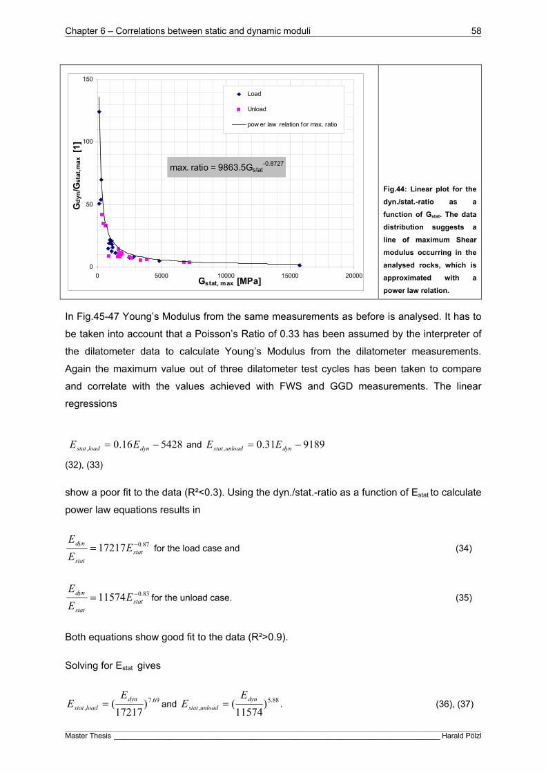
Chapter 6 – Correlations between static and dynamic moduli 58
____________________________________________________________________________________________________________________________________________________________________________________________________________
Master Thesis ________________________________________________________________________________ Harald Pölzl
max. ratio = 9863.5Gstat-0.8727
0
50
100
150
0 5000 10000 15000 20000Gstat, max [MPa]
Gd
yn/G
stat
,max
[1
]
Load
Unload
pow er law relation for max. ratio
Fig.44: Linear plot for the
dyn./stat.-ratio as a
function of Gstat. The data
distribution suggests a
line of maximum Shear
modulus occurring in the
analysed rocks, which is
approximated with a
power law relation.
In Fig.45-47 Young’s Modulus from the same measurements as before is analysed. It has to
be taken into account that a Poisson’s Ratio of 0.33 has been assumed by the interpreter of
the dilatometer data to calculate Young’s Modulus from the dilatometer measurements.
Again the maximum value out of three dilatometer test cycles has been taken to compare
and correlate with the values achieved with FWS and GGD measurements. The linear
regressions
542816.0, dynloadstat EE and 918931.0, dynunloadstat EE
(32), (33)
show a poor fit to the data (R²<0.3). Using the dyn./stat.-ratio as a function of Estat to calculate
power law equations results in
87.017217 statstat
dyn EE
E for the load case and (34)
83.011574 statstat
dyn EE
Efor the unload case. (35)
Both equations show good fit to the data (R²>0.9).
Solving for Estat gives
69.7, )
17217( dyn
loadstat
EE and 88.5
, )11574
( dynunloadstat
EE . (36), (37)

Chapter 6 – Correlations between static and dynamic moduli 59
____________________________________________________________________________________________________________________________________________________________________________________________________________
Master Thesis ________________________________________________________________________________ Harald Pölzl
Emax,load = 5E-10Edyn2.7153
Estat,load = 0.1569Edy n- 5428
R2 = 0,2321
Estat,unload = 0.3053Edy n- 9189.2
R2 = 0.2479
0
1000
2000
3000
4000
5000
6000
7000
8000
9000
10000
0 10000 20000 30000 40000 50000 60000 70000
Edyn [MPa]
Est
at,m
ax [M
Pa
] LoadUnloadpow er law relation for Emax,loadLinear (Load)Linear (Unload)
Fig.45: Static
Young’s Modulus
from dilatometer
tests in direct
comparison to
dynamic modulus
from FWS and GGD.
Data is affected by
massive scattering,
leading to poor fit of
linear regressions to
the data. For the
load case an
estimation for the
maximum occurring
Estat was assumed.
Unload: Edyn/Estat = 11574Estat-0.8296
R2 = 0.9224
Load: Edyn/Estat = 17217Estat-0.8695
R2 = 0.9509
1
10
100
1000
1 10 100 1000 10000 100000Estat, max [MPa]
Ed
yn/E
stat
,max
[1
]
Load
Unload
pow er law relation unload case
pow er law relation load case
Fig.46: Dyn./stat.-ratio as
a function of Estat. The
data shows moderate
scattering. The derived
power law equations for
load and unload case
show good fit to the data
(R²>0.90).
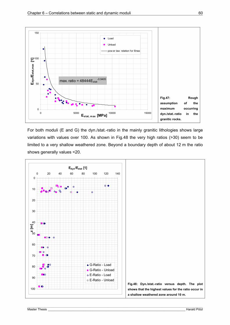
Chapter 6 – Correlations between static and dynamic moduli 60
____________________________________________________________________________________________________________________________________________________________________________________________________________
Master Thesis ________________________________________________________________________________ Harald Pölzl
max. ratio = 48444Estat-0.9405
0
50
100
150
0 5000 10000 15000Estat, max [MPa]
Ed
yn/E
stat
,max
[1
]
Load
Unload
pow er law relation for Emax
Fig.47: Rough
assumption of the
maximum occurring
dyn./stat.-ratio in the
granitic rocks.
For both moduli (E and G) the dyn./stat.-ratio in the mainly granitic lithologies shows large
variations with values over 100. As shown in Fig.48 the very high ratios (>30) seem to be
limited to a very shallow weathered zone. Beyond a boundary depth of about 12 m the ratio
shows generally values <20.
0
10
20
30
40
50
60
70
80
90
100
0 20 40 60 80 100 120 140
Edyn/Estat [1]
z [m
]
G-Ratio - Load
G-Ratio - Unload
E-Ratio - Load
E-Ratio - UnloadFig.48: Dyn./stat.-ratio versus depth. The plot
shows that the highest values for the ratio occur in
a shallow weathered zone around 10 m.

Chapter 6 – Correlations between static and dynamic moduli 61
____________________________________________________________________________________________________________________________________________________________________________________________________________
Master Thesis ________________________________________________________________________________ Harald Pölzl
In the same granitic lithology, but in another location FWS and GGD measurements were
performed beside UCS-tests and 3-axial tests (Fig.49-51). Calculated linear regressions to
derive static modulus lead to the equations
630131.03, dynaxstat EE and 87124.0, dynUCSstat EE (38), (39)
The regression for the 3-axial-tes data offers moderate fit (R²=0.61), whereas the regression
to the UCS-test data shows no significant fit to the data. Calculating power law equations for
the dyn./stat.-ratio lead to significantly improved fit to the data. The equation
72.0,
,
3945 UCSstatUCSstat
dyn EE
E (40), (41)
offers moderate fit to the data (R²=0.72) and using
73.03,
3,
4780
axstataxstat
dyn EE
E (42)
leads to a good fit with R²=0.96. Resolving for Estat results in
57.3, )
3945( dyn
UCSstat
EE for UCS-tests and 70.3
3, )4780
( dynaxstat
EE for the 3-axial tests. (43), (44)
In this data set again an assumption for the maximum occurring Estat (Fig.49) and for the
maximum occurring dyn./stat.-ratio were derived (Fig.51).
Estat,3-ax = 0.3045Edy n - 6300.8
R2 = 0,6059
Estat,UCS = 0.2435Edy n - 870.57
R2 = 0.1558
Estat,max = 0.0005Edy n1.6481
0
10000
20000
30000
40000
0 10000 20000 30000 40000 50000 60000 70000 80000
Edyn [MPa]
Est
at [M
Pa
]
UCS3-ax
lin. regression for 3-ax testlin. regression for UCS-testpow er law for Estat,max
Fig.49: Direct comparison of
dynamic Young’s Modulus
from FWS and GGD
measurements and static
modulus from UCS- and 3-axial
testing in granitic formations.
The linear regressions result in
a poor fitting relation for the
UCS-test data (R²=0.16) and a
moderate fitting 3-axial-test
data (R²=0.61).

Chapter 6 – Correlations between static and dynamic moduli 62
____________________________________________________________________________________________________________________________________________________________________________________________________________
Master Thesis ________________________________________________________________________________ Harald Pölzl
Edyn/Estat,3-ax = 4779.7Estat,3-ax-0.7332
R2 = 0.9599
Edyn/Estat,UCS = 3944.7Estat,UCS-0.7217
R2 = 0.7209
1
10
100
1000 10000 100000Estat [Mpa]
Ed
yn/E
stat
[1
] UCS
3-ax
pow er law relation for 3-ax test
pow er law relation for UCS- test
Fig.50: Logarithmic plot for
dyn./stat.-ratio as a function
of Estat for UCS-test and 3axial
tests in granites. The power
law equations derived for
dyn./stat. ratio show
moderate fit in the case of
UCS-test data and good fit for
the 3-axial-test data. In both
cases the fit is much better
than for the linear
regressions calculated in
Fig.49.
max. ratio = 6314.1Estat-0.7326
0
10
20
30
0 5000 10000 15000 20000
Estat [Mpa]
Ed
yn/E
stat
[1
]
UCS
3-ax
pow er law assumption for Emax
Fig.51: Dyn./stat.-ratio as a
function of Estat in a linear
crossplot. The curve
proposes a line for maximum
occurring Estat in the analysed
granites.
An example for moduli derived from PSSL and 3-axial measurements in a metasediment
succession (with microgabbro layers) is presented in Fig.52-54. The linear equation (Fig.52)
1214252.0 dynstat EE (45)
delivers poor fit to the data. Main reason for this bad fit seems to be a population of data
values with deviating high static moduli around 80000 MPa. These values cannot be related
to a specific rock property (for example high grade of cementing, quartz veins,…). Excluding
this values form the regression results in moderate improvement of the fit (R²=0.53). The

Chapter 6 – Correlations between static and dynamic moduli 63
____________________________________________________________________________________________________________________________________________________________________________________________________________
Master Thesis ________________________________________________________________________________ Harald Pölzl
power law approach (Fig.52) gives 75.03757 statstat
dyn EE
E
(46)
or resolved for the static modulus
4)3757
( dynstat
EE . (47)
In Fig.54 an assumption for the maximum occurring E is presented.
Estat = 0.517Edyn + 12142
R2 = 0.1026
0
20000
40000
60000
80000
100000
0 20000 40000 60000 80000 100000Edyn [MPa]
Est
at [M
Pa
]
Fig.52: Linear regression
for Estat in a linear
crossplot of dynamic
Young’s Modulus from
PSSL and static Young’s
Modulus from 3-axial
testing in a metasediment
succession with layers of
microgabbro. The linear
regression shows no
significant fit to the data,
mainly due to a (non-
rockspecific) population
of very high static moduli
(around 80000 MPa).
Edyn/Estat = 3757.1Estat-0.7546
R2 = 0.799
1
10
100
1000 10000 100000Estat [Mpa]
Ed
yn/E
stat
[1
]
Fig.53: Power law equation
for the dyn./stat.-ratio on a
logarithmic plot of
dyn./stat.-ratio as a
function of Estat. The
equation offers moderate
fit to the data.

Chapter 6 – Correlations between static and dynamic moduli 64
____________________________________________________________________________________________________________________________________________________________________________________________________________
Master Thesis ________________________________________________________________________________ Harald Pölzl
max. ratio = 2046.1Estat-0.6518
0
5
10
15
0 20000 40000 60000 80000 100000Estat [Mpa]
Ed
yn/E
stat
[1
]
Fig.54: Assumption of the
maximum occurring
dyn./stat.-ratio in the
analysed metasediments.
6.1.1 Conclusions
The direct comparison of dynamic and static moduli in (usually) shallow geotechnical
investigation areas is problematic due to massive occurring scatter in the data. Derived
empirical equations (using a linear regression in the crossplot of static modulus as a function
of dynamic modulus) offer moderate or more often poor fit to the data distributions. For this
reason another approach was tried. Power law equations were derived from the crossplot of
the dynamic/static-ratio as a function of the static modulus. This approach improved the fit of
the empirical equation to the data significantly. With one exception all the derived power law
equations could be used to estimate static moduli from dynamic ones. Table 6 gives a
summary on all derived empirical equations.
In all presented data examples an assumption for derivation of a maximum occurring
dyn./stat.-ratio, and in some cases a direct assumption of maximum static modulus occurring
in the given lithology could be derived.

Chapter 6 – Correlations between static and dynamic moduli 65
____________________________________________________________________________________________________________________________________________________________________________________________________________
Master Thesis ________________________________________________________________________________ Harald Pölzl
Litho Methods Lin. Regression R² Power Law Equation R² Solved for Estat
Siltstone
Calcarenite
CH
UCS 422005.0 dynstat EE
0.00 84.01234 stat
stat
dyn EE
E
0.31 3.6)
1234( dyn
stat
EE
Granitic Rrocks
Dilatom.
FWS 533540.0, dynloadstat GG
2411026.0, dynunloadstat GG
0.24
0.34
Load:85.06408 stat
stat
dyn GG
G
Unload:
83.04880 statstat
dyn GG
G
0.95
0.88
67.6, )
6408( dyn
loadstat
GG
67.6, )
4880( dyn
unloadstat
GG
Granitic Rocks
Dilatom.
FWS 542816.0, dynloadstat EE
918931.0, dynunloadstat EE
0.23
0.25
Load:
87.017217 statstat
dyn EE
E
Unload:
83.011574 statstat
dyn EE
E
0.95
0.92
69.7, )
17217( dyn
loadstat
EE
88.5, )
11574( dyn
unloadstat
EE
Granitic Rocks
FWS
3-ax-test
UCS-test
630131,03, dynaxstat EE
87124,0, dynUCSstat EE
0.61
0.16 72.0,
,
3945 UCSstatUCSstat
dyn EE
E
73.03,
3,
4780
axstataxstat
dyn EE
E
0.96
0.72
57.3, )
3945( dyn
UCSstat
EE
70.33, )
4780( dyn
axstat
EE
Metaseds.
Gabbro
PSSL
3-axial test 1214252,0 dynstat EE
0.10 75.03757 stat
stat
dyn EE
E
0.80 4)
3757( dyn
stat
EE
Table 6: Summary of the derived empirical relations for static moduli.

Chapter 7 – Relations between unconfined compression strength and seismic velocities 66
____________________________________________________________________________________________________________________________________________________________________________________________________________
Master Thesis ________________________________________________________________________________ Harald Pölzl
7 Relations between unconfined compression strength and seismic velocities
The unconfined compression strength (UCS) is an important and often used parameter in
geotechnics. In combination with the internal angle of friction it is used to construct failure
criteria (CHANG et al., 2006).
Correlation between strength properties and seismic velocities within a rock type is based on
some dominant influences changing both properties in a comparable direction
(SCHÖN, 2011). Increasing fracturing or porosity decreases both properties and increasing
cementation increases both properties (SCHÖN, 2011).
A correlation can be expected for a specific rock type, but not as a “general formula”. As an
example for a good correlation (see SCHÖN, 2011) the uniaxial compression strength (142
samples) and the compressional wave slowness (measured with a sonic logging tool) of fine
to medium-grained sandstone from the German Creek formation (Queensland, Australia) is
used (Fig.55). Two regressions are calculated:
linear regression 5.114050.0 pc v with R²= 0.88 (48)
power law 45.311103 pc v with R²= 0.86 (49)
0
50
100
150
1000 2000 3000 4000 5000 6000
Velocity Vp in m/s
Str
engt
h in
MP
a
Fig.55: UCS as a function of compressional wave velocity from the German Creek Formation in
Australia. The curves follow equations (48) and (49) (SCHÖN, 2011 after McN ALLY, 198*))
*): MCNALLY, G.H., 1987. Estimation of coal measures rock strength using sonic and neutron logs. Geoexploration 24, 381-
395).

Chapter 7 – Relations between unconfined compression strength and seismic velocities 67
____________________________________________________________________________________________________________________________________________________________________________________________________________
Master Thesis ________________________________________________________________________________ Harald Pölzl
According to this example the relation between seismic velocities and UCS in the given
datasets are examined in this chapter. Target is to evaluate correlations between strength
and velocity and to derive empirical relations to estimate UCS as accurate as possible from
seismic velocities.
The first example (Fig.56 and 57) involves shaly limestones and siliciclastic rocks. Seismic
velocities have been measured with PS Suspension Logger (PSSL). For siliciclastics only a
low number of UCS values could have been correlated with seismic velocities. Still it seems
that siliciclastic rocks offer lower UCS than the limestones. The estimation of UCS via
empirical relations is not possible sufficiently in this data set. Calculated linear regressions
show very low fit to the data. The use of power law relations improves the fit insignificantly to
a moderate level.
UCS= 0.0422vp - 190.23
R2 = 0.2236
UCS= 4E-18vp4.8702
R2 = 0.5968
0
100
200
300
400
500
600
5000 7500 10000 12500 15000
vp,PSSL [ft/s]
UC
S [
tsf]
Limestone
Siliciclastics
lin. regression
power law relation
UCS = 0.0602vs - 58.173
R2 = 0.2037
UCS = 1E-11vs3.537
R2 = 0.6058
0
100
200
300
400
500
600
0 2500 5000 7500 10000vs,PSSL [ft/s]
UC
S [
tsf]
Limestone
Siliciclastics
lin. regression
power law relation
Fig.56: UCS as a function
of compressional wave
velocity vp (top) and shear
wave velocity vsmeasured
with PSSL in a succession
of shaly limestones and
siliciclastics. For the
silicilastics only 2 data
values could be correlated
with velocities. Still it
seems that the
siliciclastics show much
lower UCS than the
limestones. The calculated
linear regressions show
poor fit to the data. Using
power law relations
improves the relations to a
moderate fit. There is no
significant difference
between the correlation of
UCS with vp to the
correlation with vs.
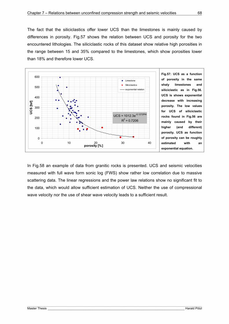
Chapter 7 – Relations between unconfined compression strength and seismic velocities 68
____________________________________________________________________________________________________________________________________________________________________________________________________________
Master Thesis ________________________________________________________________________________ Harald Pölzl
The fact that the siliciclastics offer lower UCS than the limestones is mainly caused by
differences in porosity. Fig.57 shows the relation between UCS and porosity for the two
encountered lithologies. The siliciclastic rocks of this dataset show relative high porosities in
the range between 15 and 35% compared to the limestones, which show porosities lower
than 18% and therefore lower UCS.
UCS = 1012.3e-0.1272PHI
R2 = 0.7206
0
100
200
300
400
500
600
0 10 20 30 40porosity [%]
UC
S [ts
f]
Limestone
Siliciclastics
exponential relation
Fig.57: UCS as a function
of porosity in the same
shaly limestones and
siliciclastic as in Fig.56.
UCS is shows exponential
decrease with increasing
porosity. The low values
for UCS of siliciclastic
rocks found in Fig.56 are
mainly caused by their
higher (and different)
porosity. UCS as function
of porosity can be roughly
estimated with an
exponential equation.
In Fig.58 an example of data from granitic rocks is presented. UCS and seismic velocities
measured with full wave form sonic log (FWS) show rather low correlation due to massive
scattering data. The linear regressions and the power law relations show no significant fit to
the data, which would allow sufficient estimation of UCS. Neither the use of compressional
wave velocity nor the use of shear wave velocity leads to a sufficient result.

Chapter 7 – Relations between unconfined compression strength and seismic velocities 69
____________________________________________________________________________________________________________________________________________________________________________________________________________
Master Thesis ________________________________________________________________________________ Harald Pölzl
UCS = 0.0236vp - 14.722
R2 = 0.097
UCS = 0.0002vp1.5157
R2 = 0.1426
0
100
200
300
400
500
0 1000 2000 3000 4000 5000 6000 7000
vp [m/s]
UC
S [
MP
a]
lin. regression
pow er law relation
UCS = 0.0302vs + 11.092
R2 = 0.0503
UCS = 5E-05vs1.7991
R2 = 0.1102
0
100
200
300
400
500
0 1000 2000 3000 4000 5000vs [m/s]
UC
S [
MP
a]
lin. regression
pow er law relation
Fig.58: UCS as a function
of vp (top) and vs (bottom)
measured with FWS in
granite dominated rocks.
UCS is affected by
massive scattering and
the velocity range
especially for the shear
wave is rather tight
(mainly 2000-3500 m/s),
resulting in the fact that
no sufficient empirical
relation can be derived,
which would allow
estimation of UCS from
seismic velocities.
In the dataset presented in Fig.59 seismic velocities have been measured with PSSL in a
siltstone formation. The correlation with the seismic velocities is low. Increasing velocity
increases UCS, but no sufficient equation for UCS estimation from seismic velocities could
be derived. In the plot an attempt of estimating the maximum UCS of the encountered
lithologies is presented.
For the UCS tests information about applied stress rate was also available and integrated in
the plots. The stress rate describes the increment of load increase on the sample per time
(here in MPa/min) during the UCS test until failure occurs. Three stress rate classes (0-5, 5-
10 and 10-20 MPa/min) have been defined and colour coded in the plot. It seems that
increasing the stress rate increases the measured UCS for the given siltstones.
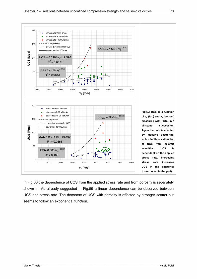
Chapter 7 – Relations between unconfined compression strength and seismic velocities 70
____________________________________________________________________________________________________________________________________________________________________________________________________________
Master Thesis ________________________________________________________________________________ Harald Pölzl
UCS = 0.0101vp - 19.596
R2 = 0.0351
UCS = 2E-07vp2.2096
R2 = 0.0843
UCSmax = 6E-27vp7.6247
0
50
100
150
200
3000 3500 4000 4500 5000 5500 6000 6500 7000
vp [m/s]
UC
S [
Mp
a]
stress rate 0-5MPa/min
stress rate 5-10MPa/min
stress rate 10-20MPa/min
lion. regression
pow er law relation for UCS
pow er law for UCSmax
UCS = 0.0184vs - 16.769
R2 = 0.0656
UCS= 0.0002vs1.5262
R2 = 0.103
UCSmax = 3E-09vs3.0824
0
50
100
150
200
0 500 1000 1500 2000 2500 3000 3500 4000
vs [m/s]
UC
S [
Mp
a]
stress rate 0-5 MPa/min
stress rate 5-10 MPa/min
stress rate 10-20 MPa/min
lin. regression
pow er law relation for UCS
pow er law for UCSmax
Fig.59: UCS as a function
of vp (top) and vs (bottom)
measured with PSSL in a
siltstone succession.
Again the data is affected
by massive scattering,
which inhibits estimation
of UCS from seismic
velocities. UCS is
dependant on the applied
stress rate. Increasing
stress rate increases
UCS in the siltstones
(color coded in the plot).
In Fig.60 the dependence of UCS from the applied stress rate and from porosity is separately
shown in. As already suggested in Fig.59 a linear dependence can be observed between
UCS and stress rate. The decrease of UCS with porosity is affected by stronger scatter but
seems to follow an exponential function.
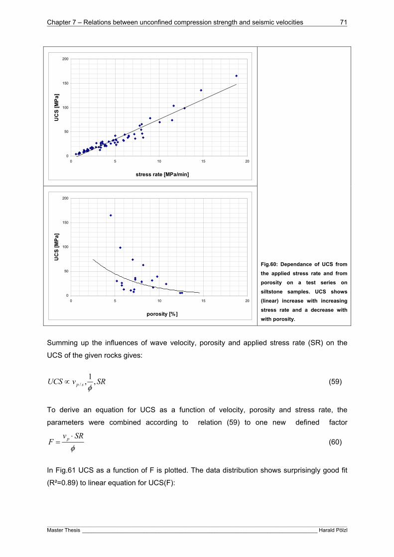
Chapter 7 – Relations between unconfined compression strength and seismic velocities 71
____________________________________________________________________________________________________________________________________________________________________________________________________________
Master Thesis ________________________________________________________________________________ Harald Pölzl
0
50
100
150
200
0 5 10 15 20
stress rate [MPa/min]
UC
S [
MP
a]
0
50
100
150
200
0 5 10 15 20
porosity [%]
UC
S [
MP
a]
Fig.60: Dependance of UCS from
the applied stress rate and from
porosity on a test series on
siltstone samples. UCS shows
(linear) increase with increasing
stress rate and a decrease with
with porosity.
Summing up the influences of wave velocity, porosity and applied stress rate (SR) on the
UCS of the given rocks gives:
SRvUCS sp ,1
,/ (59)
To derive an equation for UCS as a function of velocity, porosity and stress rate, the
parameters were combined according to relation (59) to one new defined factor
SRv
F p (60)
In Fig.61 UCS as a function of F is plotted. The data distribution shows surprisingly good fit
(R²=0.89) to linear equation for UCS(F):

Chapter 7 – Relations between unconfined compression strength and seismic velocities 72
____________________________________________________________________________________________________________________________________________________________________________________________________________
Master Thesis ________________________________________________________________________________ Harald Pölzl
82.182.0
SRv
UCS v (61) with F=f(vp [m/s], 1/Φ and SR [MPa*m/s*min]).
UCS = 0.8202F + 1.8172
R2 = 0.8855
0
50
100
150
200
0 10 20 30 40 50 60 70 80 90 100 110 120
F=SR*vp/PHI [MPa*m/min*s]
UC
S [
Mp
a]
stress rate 0-5 MPa/min
stress rate 5-10 MPa/min
stress rate 10-20 MPa/min
lin. regression for F=f(vs,SR and PHI)
Fig.61: Derivation of an
empirical “model” for UCS
in dependence of porosity,
vp and applied stress rate.
The resulting linear
function for UCS as a
function of factor F shows
surprisingly good fit to the
data.
Using shear wave velocity instead of compressional wave velocity neither increases nor
decreases the fit to the data significantly (Fig.62).
UCS = 1.4113F + 4.074
R2 = 0.8898
0
50
100
150
200
0 10 20 30 40 50 60 70
F=SR*vs/PHI [MPa*m/min*s]
UC
S [
Mp
a]
stress rate 0-5 MPa/min
stress rate 5-10 MPa/min
stress rate 10-20 MPa/min
lin. regression for F=f(vs,SR and PHI)
Fig.62: Use of shear wave
velocity for F does not
change the quality of the
derived equation
significantly.

Chapter 7 – Relations between unconfined compression strength and seismic velocities 73
____________________________________________________________________________________________________________________________________________________________________________________________________________
Master Thesis ________________________________________________________________________________ Harald Pölzl
The last example (Fig.62) shows an example of a very well fitting empirical relation for UCS
in dependence of vp measured with PSSL in calcarenites and limestones from Dubai. The fit
to the derived exponential function is excellent and the derived equation seems to be
appropriate enough to estimate UCS directly from PSSL velocities.
UCS = 2E-10vp3.1719
R2 = 0.9353
0
50
100
0 1000 2000 3000 4000 5000
vp [m/s]
UC
S [
MP
a]
power law relation for UCS
Fig.63: Very well fitting empirical
equation for UCS as a function of vp
measured with PSSL in calcarenites and
limestones.

Chapter 7 – Relations between unconfined compression strength and seismic velocities 74
____________________________________________________________________________________________________________________________________________________________________________________________________________
Master Thesis ________________________________________________________________________________ Harald Pölzl
7.1.1 Conclusions
In the presented data examples only one case shows well correlating UCS with seismic
velocities. In all other cases no sufficient correlation for a derivation of an empirical equation
for estimation of UCS from seismic velocities could be found.
One important influencing factor for UCS is the porosity of the analysed rocks. UCS is highly
sensitive to porosity. Increasing porosity leads to exponential decrease of UCS.
Also an important role for measured UCS plays the applied stress rate during the tests.
Between UCS and stress rat a clear linear dependence was found in one of the data
examples. It was possible to derive an equation for UCS as a function of porosity, velocity
and stress rate.

Chapter 8 – Conclusions and discussion 75
____________________________________________________________________________________________________________________________________________________________________________________________________________
Master Thesis ________________________________________________________________________________ Harald Pölzl
8 Conclusions and discussion
Deformation moduli of soil and rock are important parameters for geotechnical site
investigations and design. Static methods are well established in geotechnics and are seen
to offer reliable modulus values over a broad range of stress and strain, whereas dynamic
moduli are restricted to very small strains. Static methods are often costly and time
consuming compared to dynamic methods that can provide investigation of larger volumes at
a reasonable amount of time and money. To overcome the disadvantages and to combine
the advantages of both approaches, it was tried to find correlations between static and
dynamic moduli with the intention to find reliable empirical relations to extend the static point
information to larger volumes.
In a first step it was intended to perform a direct comparison of different static and different
dynamic measurement techniques to get an idea of how congruent (or incongruent) different
static and different dynamic results are. A direct comparison of static methods was
unfortunately not possible due to lack of “data intersection”. Different static methods have not
been applied in the same location/borehole in the given data sets.
The comparison of wave velocities measured with different dynamic methods shows that
generally small differences between velocities from different methods occur. These
differences are mainly caused by different measurement frequencies and different
resolutions and occur especially between non invasive surface methods like the spectral
analysis of surface waves and borehole methods like full wave form sonic logging or PS
Suspension Logging. An exception from this trend seems to be the downhole seismic
method. Velocity values obtained with downhole seismics show good correlation with other
methods in some sections, but also low or no correlation in other sections. This is seen to be
mainly caused by the fact that source receiver offset is increasing during measurements
leading to an increase of wave energy attenuation especially of high frequencies with
increasing investigation depth resulting in difficulties in accurate and distinct first arrival
determination. Therefore PS Suspension Logging for soils and unconsolidated materials and
full waveform sonic logging in rocks, providing constant source receiver offset should be
preferred if the borehole conditions (fluid filled, open hole and acceptable hole inclination)
allow this measurements.
Beside the availability of density values, the determination of shear wave velocity is often the
limiting factor for the dynamic methods, especially for full waveform sonic and PS
Suspension Logging. For this reason it was tried to estimate shear wave velocities from vp/vs
crossplots. This site and lithology specific approach offered moderate to poor success. Only
crosshole measurements seem to provide sufficient data quality for accurate shear wave
velocity estimations in rocks as well as in unconsolidated materials. For other methods the fit

Chapter 8 – Conclusions and discussion 76
____________________________________________________________________________________________________________________________________________________________________________________________________________
Master Thesis ________________________________________________________________________________ Harald Pölzl
of derived equations to the given data distributions was generally moderate to poor. An
appropriate estimation of vs is therefore not recommended.
The correlation between static and dynamic moduli showed that in shallow geotechnical
investigations the ratio of dynamic over static modulus can range over two or three decades.
The dynamic modulus can reach values that are 100 times the static one. Static methods
cover a broad stress and strain range and are (or can be) performed until material failure.
Therefore also non elastic deformation processes can be analysed. The dynamic methods
offer measurements in a very small strain area and cover only elastic deformations resulting
in higher dynamic moduli. Beside these fundamental differences, weathering seems to be an
important factor for massive increases of the dynamic/static ratio.
The direct correlation between static and dynamic moduli to derive linear relationships for
estimation of static moduli did not provide sufficient results. The derived equations offered
poor or no fit to the given data distributions, which were affected by massive scattering. A
result that could be obtained from the direct approach in nearly all cases is a derivation of
maximum occurring static modulus of the site or the investigated lithology.
To increase the quality of empirical relations for the static parameters an indirect approach
was selected. The dynamic/static ratio was plotted as a function of static modulus. This
approach decreased the scattering in the data distributions for all presented examples. The
derived equations for the ratio as a function of static modulus were solved for the static
modulus. In all examples the fit of derived equations was increased successfully with this
approach (compared to the linear approach). Except two examples R² was raised to values
above or equal to 0.80 indicating good to excellent fit to the data.
Because of abundant data for the unconfined compression strength, correlations between
this strength property and acoustic velocities were included in this report. Relating UCS only
to the wave velocities did generally not provide sufficient relations, because of massive
scattering in the data distributions. Only one case was found, where PSSL velocities can be
used to estimate UCS accurate enough. Similar to the linear modulus correlation, only a
function for maximum occurring UCS in the investigated lithologies could be derived.
In one example additional information about porosity and applied stress rate were included in
the analysis. Seismic velocity, porosity and stress rate were combined to a new factor F and
plotted against the UCS, resulting in a good linear correlation between F and UCS. Involving
porosity and stress rate would allow relative accurate estimation of UCS.

Chapter 9 – Indices 77
____________________________________________________________________________________________________________________________________________________________________________________________________________
Master Thesis ________________________________________________________________________________ Harald Pölzl
9 Indices
9.1 References
BARTON, N., 2007. Rock quality, seismic velocity, attenuation and anisotropy. Taylor & Francis
Group, London, UK, 2007, 729 p.
BATZLE, M. and WANG, Z., 1992. Seismic properties of pore fluids. Geophysics 57 (11), p. 1396-
1408.
BOYER, S., MARI, J.-L., 1997, Oil and Gas Exploration Techniques: Seismic Surveying and Well
Logging. Editions Technip, Paris, 1997, 192 p.
CASTAGNA, J.P., BATZLE, M.L., EASTWOOD, R.L., 1985. Relationships between compressional-
wave and shear wave velocities in clastic silicate rocks. Geophysics 50, p. 571-581.
CASTAGNA, J.P., BATZLE, M.L., KAN, T.K., 1993. Rock Physics – The link between rock properties
and AVO response. In: CASTAGNA, J.P., BACKUS, M.L.(eds.),Offset-Dependant Reflectivity –
Theory and Practice of AVO analysis. Investigations in Geophysics, 8, 348 p.
CHANG, C., ZOBACK, M.D., KHAKSAR, A., 2006. Empirical relations between rock strength and
physical properties in sedimentary rocks. Journal of Petroleum Science and Engineering, Vol. 51,
Elsevier 2006, p. 223-237.
DE VALLEJO, G. and FERRER, M., 2011. Geological engineering. CRC Press, Balkema, Boca Raton,
2011, 678 p.
ELLIS E.V., SINGER J.M., 2007, Well Logging for Earth Scientists. 2nd Edition, Springer Verlag,
Dortrecht, 2007, p.247-322.
FJAER E., HOLT R.M., HORSRUD P., RAAEN A.M. AND RISNES R., 1992, Petroleum related rock
mechanics. Developments in Petroleum Science, Vol. 33, Elsevier, 1992, 338p.
HALDORSEN J. B. U., JOHNSON D. L., PLONA T., SINHA B., VALERO H.-P., WINKLER K.,
Borehole Acoustic Waves, Oilfield Review, 2006, p. 34-43.
HAN, D., NUR, A. and MORGAN, D., 1986. Effects of porosity and clay content on wave velocities in
sandstones. Geophysics, 51 (11), p. 2093-2107.
HELBIG, K., 1992. Coordinate-free representation of the elastic tensor. EAGE 54th Meeting and
Technical Exhibition, Paris, 1-5 June, paper A049.

Chapter 9 – Indices 78
____________________________________________________________________________________________________________________________________________________________________________________________________________
Master Thesis ________________________________________________________________________________ Harald Pölzl
HORSRUD, P., 2001. Estimating mechanical properties of shale from empirical correlations. SPE drill.
Complet. 16, 68-73.
KING, M.S., SHAKEEL, A. AND CHAUDRY N.A., 1997, Acoustic wave propagation and permeability
in sandstones with systems of aligned cracks. IN: LOVELL, M.A. AND HARVEY, P.K. (eds), 1997,
Developments in Petrophysics, Geological Society Special Publication No. 122, p. 69-85.
LAMA, R.D. AND VUTUKURI, V.S., 1978, Handbook on Mechanical Properties of rocks – Testing
Techniques and results, Volume II. In: Series on rock and soil mechanics, Vol.3, No.1, 1978, Trans
Tech S.A., Switzerland, 1978, 481p.
LOOK, B., 2007.Handbook of Geotechnical Investigation and Design Tables.Taylor&Francis Group,
London (and others), 2007, 331p.
LUNNE T., ROBERTSON P.K., POWELL J.J.M., 1997, Cone Penetration testing in Geotechnical
Practice. Blackie Acad. & Professional, London, 1997, p.179-181.
MAVKO,G., MUKERJI and DVORKIN, J., 1998. The rock physics handbook. Tools for seismic
analysis in porous media. Cambridge University Press, first published 1998, 329p.
MOGI, K., 2007, Experimental Rock Mechanics. In: Kwasniewski, A.M. (editor in chief), 2007,
Geomechanics Research Series Vol. 3. Taylor&Francis Group, London, UK, 2007, p. 3-193.
SCHÖN, J., 1983, Petrophysik. Physikalische Eigenschaften von Gesteinen und Mineralen. Ferdinand
Enke Verlag Stuttgart, 1983, p.349ff.
SCHÖN J.H., 1996, Physical properties of rocks: fundamentals and principles of petrophysics.
Handbook of geophysical exploration, Seismic Exploration, Vol. 18, K. Helbig and S. Treitel (eds.),
Pergamon Press London , 1996, 1st edition, p.133-273.
SCHÖN J.H., 2011, Physical properties of rocks: A workbook. Handbook of petroleum exploration and
production, Vol. 8, CUBITT, J. (series editor), Elsevier, 2011, p149-272.
TELFORD, W.M., GELDART, L.P., SHERIFF, R.E., Applied geophysics, Second Edition, reprint 2004.
Cambridge University Press, first published 1990, p.149ff.
THOMSEN, L., 1986. Weak elastic anisotropy. Geophysics 51 (10), p.1954-1967.
WHITE J.E., 1983, Underground Sound, application of seismic waves. Methods in Geochemistry and
Geophysics, 18, Elsevier Science Publishers B.V., 1983, 253p.

Chapter 9 – Indices 79
____________________________________________________________________________________________________________________________________________________________________________________________________________
Master Thesis ________________________________________________________________________________ Harald Pölzl
WIDARSONO, B., MARSDEN, J.R. AND KING, M.S., 1998, In situ stress prediction using differential
strain analysis and ultrasonic shear wave splitting. In: HARVEY, P.K. AND LOVELL, M.A. (eds) Core-
Log Integration, Geological Society, London, Special Publications, 136, p. 185-195.
ZHANG, L., 2005. Engineering properties of rocks. Elsevier geo-engineering book series, Vol. 4,
Elsevier, Amsterdam, 2005, 290 p.
9.2 Tables
Table 1: Table of useful transformations and conversions (SCHÖN, 2011). ...........................6
Table 2: Empirical equations for shear wave velocity from literature. ....................................27
Table 3: Empirical Relations between static and dynamic moduli after literature ..................30
Table 4: Overview on sites, dominant lithologies and methods .............................................34
Table 5: Empirical relations for different sites and lithologies sorted after their R² value. ......45
Table 6: Summary of the derived empirical relations for static moduli. ..................................65
9.3 Figures
Fig.1: Stress-strain curve (MOGI, 2007) ..................................................................................8
Fig.2: Stress-Strain curve approaches to derive deformation moduli (after ZHANG, 2005). ...8
Fig.3: E as a function of strain for different lithologies (MOGI, 2007).......................................9
Fig.4: Slope behaviour yield stress for different stress states (MOGI, 2007). ........................10
Fig.5: Compressional and shear wave propagation characteristics (BARTON, 2007)...........12
Fig.6: Propagation of waves in boreholes, (HALDORSEN et al., 2006).................................14
Fig.7: Snellius' law applied on waves an ray tracing (HALDORSEN et al., 2006)..................15
Fig.8: Propagation of Surface Waves.....................................................................................17
Fig.9: TOP Anisotropy in rock material (: BARTON, 2007); (HALDORSEN et al., 2006).......18
Fig.10: Shear wave splitting (from BARTON, 2007)...............................................................21
Fig.11: Different lithologies and their acoustic wave velocity (SCHÖN, 2011).......................22
Fig.12: vp as a function of saturation and hydrostatic pressure (Barton, 2007)......................25
Fig.13: Example of depandance of shear modulus of the strain level (LOOK, 2007). ...........28
Fig.14: Relation between static and dynamic moduli (SCHÖN, 2011)...................................29
Fig.15: Relation between the stat./dyn. ratio and the static modulus (after SCHÖN, 2011). .29
Fig.16: Young's modulus for granite (from SCHÖN, 2011; after BELIKOV et al., 1970.........29

Chapter 9 – Indices 80
____________________________________________________________________________________________________________________________________________________________________________________________________________
Master Thesis ________________________________________________________________________________ Harald Pölzl
Fig.17: Empirical Equations for UCS-estimation (CHANG et al., 2006). ................................32
Fig.18: Empirical Equations for UCS estimation of shales (CHANG et al., 2006)..................32
Fig.19: Empirical Equations for UCS estimation of limestones and dolomites CHANG et al.,
2006). ..............................................................................................................................33
Fig.20: Empirical Equations for UCS estimation of siliciclastic rocks from internal angle of
friction (CHANG et al., 2006). .........................................................................................33
Fig.21: Direct comparison of shear wave velocity measurements with PSSL, MASW and
downhole seismics. .........................................................................................................36
Fig.22: Direct comparison of vp from downhole and PSSL-measurements and vs from
downhole, PSSL and splitted shear wave crosshole measurements..............................37
Fig.23: Velocity crossplot to compare shear wave velocities measured with PSSL and
crosshole measurements. ...............................................................................................38
Fig.24: Velocity of vs,hv as a function of vs,hh. ..........................................................................39
Fig.25: vp-vscrossplot for downhole and PSSL velocities .......................................................40
Fig.26: Direct comparison of downhole and PSSL measurements ........................................41
Fig.27: Comparison of shear wave velocity from laboratory transmission and PSSL ............42
Fig.28: Comparison of shear wave velocities measured with PSSL and lab-data ................42
Fig.29: vp-vs crossplot for different methods and lithologies ...................................................44
Fig.30: Empirical relations for vs of a layered succession of shale.........................................46
Fig.31: Empirical relation for vs of a shale succesion .............................................................47
Fig.32: Empirical relation for vs of plutonic rocks....................................................................48
Fig.33: Velocity crossplot for FWS measurements ................................................................49
Fig.34: Velocity crossplot for crosshole seismic measurements in siltstone-calcsiltite. .........50
Fig.35: Velocity crossplot for PSSL-measurements in metasediments and gabbros.............50
Fig.36: Velocity crossplot for partly cemented sands .............................................................51
Fig.37: vp-vs crossplot for soils................................................................................................52
Fig.38: Velocity crossplot for different unconsolidated materials ...........................................52
Fig.39: direct comparison between Edyn and Estat ...................................................................55
Fig.40: dynamic/static ratio as a function of Estat. ...................................................................55
Fig.41: Linear plot for dnyamic/static ratio as a function of Estat.. ...........................................56
Fig.42: Direct comparison of dynamic and static Shear Modulus from dilatometer tests and
FWS ................................................................................................................................57
Fig.43: Logarithmic plot for dyn./stat.-ratio as a function of static Shear Modulus. ................57

Chapter 9 – Indices 81
____________________________________________________________________________________________________________________________________________________________________________________________________________
Master Thesis ________________________________________________________________________________ Harald Pölzl
Fig.44: Linear plot for the dyn./stat.-ratio as a function of Gstat...............................................58
Fig.45: Static Young’s Modulus from dilatometer tests in direct comparison to dynamic
modulus from FWS and GGD.. .......................................................................................59
Fig.46: Dyn./stat.-ratio as a function of Estat............................................................................59
Fig.47: Rough assumption of the maximum occurring dyn./stat.-ratio in the granitic rocks. ..60
Fig.48: Dyn./stat.-ratio versus depth ......................................................................................60
Fig.49: Direct comparison of dynamic Young’s Modulus from FWS and GGD measurements
and static modulus from UCS- and 3-axial testing in granitic formations........................61
Fig.50: Logarithmic plot for dyn./stat.-ratio as a function of Estat for UCS-test and 3axial tests
in granites........................................................................................................................62
Fig.51: Dyn./stat.-ratio as a function of Estat in a linear crossplot............................................62
Fig.52: Linear regression for Estat. ..........................................................................................63
Fig.53: Power law equation for the dyn./stat.-ratio. ................................................................63
Fig.54: Assumption of the maximum occurring dyn./stat.-ratio ..............................................64
Fig.55: UCS as a function of wave velocity (SCHÖN, 2011 after McN ALLY, 1987*))............66
Fig.56: UCS as a function of compressional wave velocity vp................................................67
Fig.57: UCS as a function of porosity.....................................................................................68
Fig.58: UCS as a function of vp and vs measured with FWS in granite ..................................69
Fig.59: UCS as a function of vp and vs measured with PSSL in siltstone..............................70
Fig.60: Dependance of UCS from the applied stress rate and from porosity .........................71
Fig.61: UCS in dependance of porosity, vp and applied stress rate. ......................................72
Fig.62: Use of shear wave velocity for F ................................................................................72
Fig.63: UCS as a function of vp measured with PSSL in calcarenites and limestones...........73

Appendix I
____________________________________________________________________________________________________________________________________________________________________________________________________________
Master Thesis ________________________________________________________________________________ Harald Pölzl
Appendix
Description of involved methods
Seismic Surface Waves - Spectral Analysis of Surface Waves (SASW)
Method description SASW uses Surface Wave (especially Rayleigh Wave) dispersion to
evaluate shear wave velocity and shear modulus profiles. About 2/3 of
the energy produced by seismic sources are imparted into Rayleigh
waves (also “ground roll”), which show very high dependence on shear
wave velocity of the ground. Dispersion means that different frequency
components of the surface wave travel at different velocities (phase
velocity) in a layered medium. According to that the use of a wide
frequency range allows sampling of different portions of the ground.
High frequencies (wavelengths shorter than the top layer thickness)
propagate only through surface layers, whereas lower frequencies also
propagate through deeper soils. SASW uses a pair of receivers
(velocity transducers or accelerometer), which is configured according
to the frequency range that should be detected. Vibrations of known
frequency travel from source to receiver along the surface, are
recorded, digitized and transformed into frequency domain via Fast
Fourier Transformation.
Fig.64: Scheme of a
common mid point
(CMP) geometry spread
used for SASW
measurements. Source
receiver distances and
receiver spacings ar
increased in steps (from
STOKOE et al., 1994).
The source is normally used in a forward and reverse position. The
result of the measurements is a dispersion curve, plotting phase
velocity versus frequency or wavelength. To obtain shear wave velocity
profiles an iterative inversion is applied, including estimations of
Poisson’s Ratio, layer thickness and density.

Appendix II
____________________________________________________________________________________________________________________________________________________________________________________________________________
Master Thesis ________________________________________________________________________________ Harald Pölzl
System data Spacing typically 0.5 m, 1 m, 2 m, 4 m, 8 m, 16 m, 32 m
and 64 m
Vertical resolution low to medium, controlled by local properties
(velocity contrasts, layer thickness,…). Rule of
thumb: Layer thickness should be at least 1/5 of
its depth to be resolved.
frequency low (several to several tens of Hz)
investigated volume high
Seismic Sources for spacings up to 8 m: (sledge) hammers,
dropped weights up to 70 kg.
For spacings above 8 m: dropped weights
up to 900 kg, bulldozers or large dynamic
compaction weights
Formation Preferred soils. Receiver coupling and source energy transmission
must be possible.
Depth limit PARK et al, 2007: generally 10 to 30 m with possibility of site specific
variations
Parameters measured travel time of surface waves with a known frequency
calculated velocities of s-waves
Measuring progress medium to high
Comment Problems for SASW:
- Near field effects of surface waves that travel only short distances
from the source (non planar wave geometry)
- The use of only a pair of receivers may lead to difficulties in
distinguishing between noise and signal
- Far field effects caused by attenuation of higher frequencies and
noise contamination at higher offsets
- Stiff over soft layers
- Stiff Sides overlaid by water
- Gravity effect leading to increased surface wave velocities in very
soft undergrounds and at very large wavelengths. STOKOE et al.,
1994 calculate the critical wavelength, where gravity starts to play a
role with: 2
2
2
2
)(1
2
p
s
scritical
v
v
v
- Inversion of dispersion curves requires preliminary knowledge of
underground conditions.
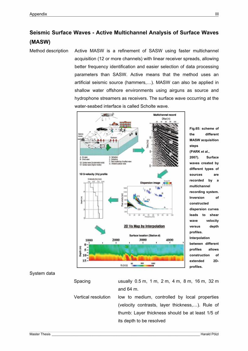
Appendix III
____________________________________________________________________________________________________________________________________________________________________________________________________________
Master Thesis ________________________________________________________________________________ Harald Pölzl
Seismic Surface Waves - Active Multichannel Analysis of Surface Waves
(MASW)
Method description Active MASW is a refinement of SASW using faster multichannel
acquisition (12 or more channels) with linear receiver spreads, allowing
better frequency identification and easier selection of data processing
parameters than SASW. Active means that the method uses an
artificial seismic source (hammers,…). MASW can also be applied in
shallow water offshore environments using airguns as source and
hydrophone streamers as receivers. The surface wave occurring at the
water-seabed interface is called Scholte wave.
Fig.65: scheme of
the different
MASW acquisition
steps
(PARK et al.,
2007). Surface
waves created by
different types of
sources are
recorded by a
multichannel
recording system.
Inversion of
constructed
dispersion curves
leads to shear
wave velocity
versus depth
profiles.
Interpolation
between different
profiles allows
construction of
extended 2D-
profiles.
System data
Spacing usually 0.5 m, 1 m, 2 m, 4 m, 8 m, 16 m, 32 m
and 64 m.
Vertical resolution low to medium, controlled by local properties
(velocity contrasts, layer thickness,…). Rule of
thumb: Layer thickness should be at least 1/5 of
its depth to be resolved

Appendix IV
____________________________________________________________________________________________________________________________________________________________________________________________________________
Master Thesis ________________________________________________________________________________ Harald Pölzl
frequency Low (several to several tens of Hz)
investigated volume medium to high
Seismic Sources for spacings up to 8 m: (sledge) hammers,
dropped weights up to 70 kg.
For spacings above 8 m: dropped weights up to
900 kg, bulldozers or large dynamic compaction
weights, VIBROSEIS and airguns for offshore
applications.
Formations Preferred soils. Receiver coupling and source energy transmission
must be possible.
Depth limit PARK et al, 2007: generally 10 to 30 m with possibility of site specific
variations.
Parameters measured travel time of surface waves with a known frequency
calculated velocities of s-waves
Measuring progress medium to high
Comment The use of only a pair of receivers may lead to difficulties in
distinguishing between noise and signal
Problematic cases for MASW:
- Near field effects for surface waves that travel only short distances
(low offset) from the source (non planar wave geometry)
- Far field effects caused by attenuation of higher frequencies and
noise contamination at higher offsets
- Stiff over soft layers
- Stiff Sites overlaid by water
- Gravity effect leading to increased surface wave velocities in very
soft undergrounds and at very large wavelengths. STOKOE et al.,
1994 calculate the critical wavelength, where gravity starts to play a
role with : 2
2
2
2
)(1
2
p
s
scritical
v
v
v
- Tide and currents in the offshore environment have to be respected
while planning MASW offshore profiles.

Appendix V
____________________________________________________________________________________________________________________________________________________________________________________________________________
Master Thesis ________________________________________________________________________________ Harald Pölzl
Seismic Surface Waves - Refraction Micro Tremor (ReMi), Passive and
Interferometric Multichannel Analysis of Surface Waves (MASW)
Method description Refraction Microtremor or Microtremor Survey Method and passive MASW
are generally working like the SASW and MASW method. Passive means
that surface waves are not generated by artificial seismic sources but by
cultural (traffic,…) or natural activities (tidal motion,…). PARK et al., 2007
distinguish two different methods of passive MASW; the passive remote
MASW and the passive Roadside MASW: A recent development on the field
of surface wave methods is the Interferometric MASW, which uses slowness-
frequency slant-stack analysis combined with interferometric time-domain
dispersion analysis to improve resolution and maximum investigation depth of
MASW.
Fig.66: Passive MASW-methods
and their measurement
geometries. Passive remote
MASW can use any symmetric
receiver array (PARK et al., 2007).
The passive remote MASW can use any symmetric receiver array for
data acquisition, whereas the roadside method uses linear arrays. The
combination of active and passive methods can enlarge the analyzable
frequency.
Comment Combination of active and passive surface wave methods can improve
quality of results.
For further information on interferometric MASW Daniel R. H.
O’Connell and James P. Turner (Fugro Will Lettis & Associates, Inc)
should be contacted.

Appendix VI
____________________________________________________________________________________________________________________________________________________________________________________________________________
Master Thesis ________________________________________________________________________________ Harald Pölzl
References
STOKOE K.H., WRIGHT, S.G., BAY, J.A., ROESSET, J.M., 1994. Characterization of geotechnical
sites by SASW method. IN: Geophysical Characterization of Sites, Volume prepared by ISSMFE
Technical Committee #10 for XIII ICSMFE, 1994, New Delhi, India. Edited by Richard D. WOODS,
International Science Publisher, New York, 1994, p.15-25.
PARK B.C., Miller R.D., Jianghai X., 1999, Multichannel analysis of surface waves, Geophysics,
Vol.64, No. 3, May-June 1999, p.800-808.
PARK., B.C., MILLER, R.D., XIA, J. and IVANOV, J., 2007. Multichannel analysis of surface waves
(MASW) – active and passive methods. The leading edge, January 2007, p. 60-64.
ANDERSON N., CHEN G., KOCIU S., LUNA R., THITIMAKORN T., MALOVICHO A., MALOVICHKO
D., SHYLAKOV D., 2003, Final report RDT 03-006, Vertical Shear-Wave Velocity Profiles Generated
From Spectral Analysis Of Surface Waves: Field Examples. Prepared for Missouri Departement of
Transportation, Research, Development and Technology, Jefferson City, Missouri, April 2003.
O’CONNELL, D.R.H. and TURNER, J.P., 2011. Interferometric Multichannel Analysis of Surface
Waves (IMASW). Bulletin of the seismological society of America, 10/2011, Vol. 101, p.2122-2141.
Borehole Extension Testing
Method description This kind of tests uses devices in prebored holes in soils and rock.
Many tools use drilled pockets of a smaller diameter than the main
hole. Lengths of this pockets vary usually between 1.5 m and 3.0 m.
The devices are lowered down to the wished depth and apply pressure
on the borehole wall. The resulting deformation is measured.
“Seitendrucksonden” use hydraulic cylinders for load application and
electrical distance measurement, the Menard Probe or Pressuremeter
uses tube packers and volumetric borehole extension measurement
and Dilatometers use tube packers combined with electrical distance
measurement. The tests can comprise between 2 to 14 circles of
loading and unloading at one depth. The maximum applied pressure
depends on the building planned or is reached when the rock formation
fails or the loading limit of the tool is reached. From the recorded stress
strain diagram the mechanical properties can be derived.

Appendix VII
____________________________________________________________________________________________________________________________________________________________________________________________________________
Master Thesis ________________________________________________________________________________ Harald Pölzl
Fig.67: Example
for a Menard
Probe and its
use in a
borehole
(SCHNAID,
2009).
For the analysis cycles after onset of plasticity (if reached) are
preferred. To derive the shear modulus 3 parts of the pressure-
deformation curve are interesting:
- The initial slope of the elastic loading phase (initial shear modulus)
- The slope of the chord bisecting small rebound cycles
- The slope f the first part of the contraction curve
For the reason that strain-stiffness relationships are not strictly linear
more comprehensive interpretation methods have been developed,
looking at smaller steps of the curve and not the extreme ends of the
cycles.
Fig.68: Load-Unload Loop and
estimation of deformation modulus
from the loop (SCHNAID, 2009).
Fig.69: Load-Unload
Loops and
interpretation of
pressuremeter tests
in coal (FUGRO
internal material).
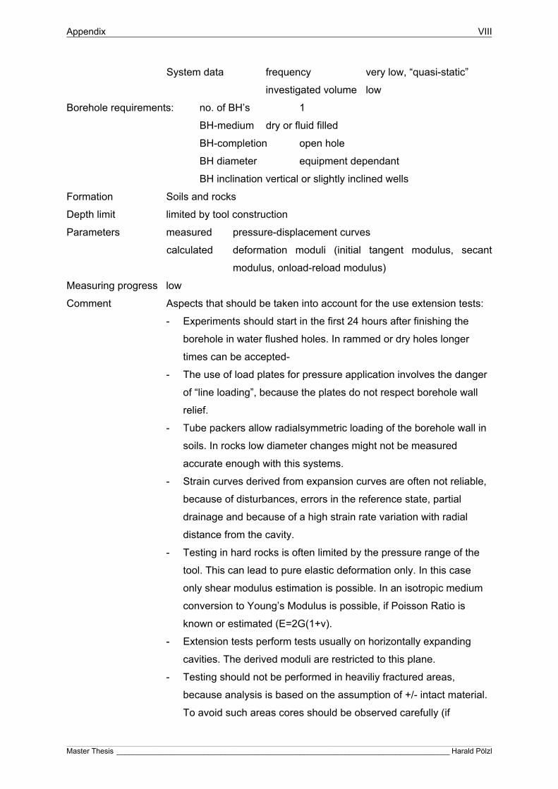
Appendix VIII
____________________________________________________________________________________________________________________________________________________________________________________________________________
Master Thesis ________________________________________________________________________________ Harald Pölzl
System data frequency very low, “quasi-static”
investigated volume low
Borehole requirements: no. of BH’s 1
BH-medium dry or fluid filled
BH-completion open hole
BH diameter equipment dependant
BH inclination vertical or slightly inclined wells
Formation Soils and rocks
Depth limit limited by tool construction
Parameters measured pressure-displacement curves
calculated deformation moduli (initial tangent modulus, secant
modulus, onload-reload modulus)
Measuring progress low
Comment Aspects that should be taken into account for the use extension tests:
- Experiments should start in the first 24 hours after finishing the
borehole in water flushed holes. In rammed or dry holes longer
times can be accepted-
- The use of load plates for pressure application involves the danger
of “line loading”, because the plates do not respect borehole wall
relief.
- Tube packers allow radialsymmetric loading of the borehole wall in
soils. In rocks low diameter changes might not be measured
accurate enough with this systems.
- Strain curves derived from expansion curves are often not reliable,
because of disturbances, errors in the reference state, partial
drainage and because of a high strain rate variation with radial
distance from the cavity.
- Testing in hard rocks is often limited by the pressure range of the
tool. This can lead to pure elastic deformation only. In this case
only shear modulus estimation is possible. In an isotropic medium
conversion to Young’s Modulus is possible, if Poisson Ratio is
known or estimated (E=2G(1+v).
- Extension tests perform tests usually on horizontally expanding
cavities. The derived moduli are restricted to this plane.
- Testing should not be performed in heaviliy fractured areas,
because analysis is based on the assumption of +/- intact material.
To avoid such areas cores should be observed carefully (if

Appendix IX
____________________________________________________________________________________________________________________________________________________________________________________________________________
Master Thesis ________________________________________________________________________________ Harald Pölzl
available), optical or acoustic borehole imagers can be run or sonic
logging (FWS or PSSL) can help. Also caliper logs can help to
avoid testing in zones where the borehole diameter is highly
different from the nominal diameter.
- Exact placement of the tool is a critical point in pressuremeter
testing. Core descriptions/photos and/or image logs and/or caliper
logs can improve tool positioning.
- Unconsolidated materials are highly disturbed through drilling
processes:
References
FECKER E., 1997, Geotechnische Meßgeräte und Feldversuche im Fels. Hrsg.: Edwin Fecker, 1997,
Ferdinand Enke Verlag, Stuttgart, p.133-171.
LUNNE T., ROBERTSON P.K., POWELL J.J.M., 1997, Cone Penetration testing in Geotechnical
Practice. Reprinted by E&FN Spon, London, 1997, p.179-181.
SCHNAID, F., 2009. In-situ testing in geomechanics, the main tests. Taylor&Francis, London, 2009,
329 p.
HUNT, R.E., 2005. Geotechnical engineering investigation handbook. Tayor&Francis, CRC, Boca
Raton, 2005, 1066 pages.
Full Waveform Sonic Log (FWS)
Method description The Sonic Log transmits a sonic signal and generates a p-wave in the
borehole fluid. The p-wave radiates away from the transmitter in all
directions and strikes the borehole wall. Some of the energy will
propagate still as p-wave, some of it is converted into an s-wave.
These waves generate elementary waves in each position radiating
back at the critical angle of refraction and hit the receivers (receiver
arrays with at least 2 receivers) located on the tool at defined
distances. From the differences in travel time at the receivers and the
tool geometry p- and s-wave velocities are calculated.

Appendix X
____________________________________________________________________________________________________________________________________________________________________________________________________________
Master Thesis ________________________________________________________________________________ Harald Pölzl
Fig.70: Principle of a FWS-tool. The
energy emitted by a source is
recorded by a series of receivers. In
geotechnical applications typically
2-4 receivers are used (Picture from
HALDORSEN et al., 2006).
The wave velocities can be obtained by direct manual picking of wave
arrivals in the receiver data and by calculating the velocities from
traveltime differences between the receivers (spacing is well defined).
Another possibility is extracting the wave velocities via cross
correlation using semblance algorithms.
Fig.71: Example for a FWS record and a calculated Semblance cross correlation. The
record consists of 4 receivers (R1-R4) that record the whole wavetrain. Spacings for this
system are 0.6 m, 0.8 m 1.0 m and 1.2 m. The semblance gives correlation maximums for
the p-wave (red arrow) and for the s-wave (blue arrow). The broad maximum at the right
end includes a correlation maximum for the Stoneley wave (Fugro internal material).

Appendix XI
____________________________________________________________________________________________________________________________________________________________________________________________________________
Master Thesis ________________________________________________________________________________ Harald Pölzl
System data spacing constant (typically 0.5m – 1.5m)
vertical resolution high and constant (≈spacing)
sampling interval high and constant (typically 5cm – 10cm)
frequency high (typically 5kHz - 20kHz)
investigated volume small and constant
Borehole requirements no. of BH 1
BH medium water or drilling mud
BH completion open borehole
BH inclination 90° - 30° from horizontal
Formation limited to formations with vp >1500m/s (usually consolidated materials
and rocks)
Depth limit limited by logging cable or pressure rating of downhole tool
Parameters measured travel time of acoustic waves
calculated velocities of p- and s-waves
Measuring progress high (typical vertical logging speed is 4 m/min)
Comment Aspects that should be taken into account for the use of FWS:
- FWS needs fluid filled and open boreholes.
- FWS is highly dependant on the borehole conditions. Massively
fractured zones, wall breakouts, soft layers, fault gauges, etc. can
be the cause for data gaps in compressional and shear wave
velocity data.
- FWS does not work properly in unconsolidated materials or soils.
References
HALDORSEN J. B. U., JOHNSON D. L., PLONA T., SINHA B., VALERO H.-P., WINKLER K.,
Borehole Acoustic Waves, Oilfield Review, 2006, p34-43.
ELLIS E.V., SINGER J.M., 2007, Well Logging for Earth Scientists. 2nd Edition, Springer Verlag,
Dortrecht, 2007, p.247-322.

Appendix XII
____________________________________________________________________________________________________________________________________________________________________________________________________________
Master Thesis ________________________________________________________________________________ Harald Pölzl
PS-Suspension Log (PSSL)
Method description PSSL is using a single downhole probe, suspended by a cable
containing a combined reversibly horizontal solenoid source and two
biaxial geophones, separated by a flexible isolation tube. It is intended
to provide relative low frequency measurements of traveltimes of p-
and horizontal polarised, vertical propagating shear waves.
Fig.72: Functional
units and
measurement
geometry of the
PSSL tool (FUGRO
internal material).
The source is activated in two opposite directions for generation of p-
and horizontal polarised s-waves (in reality it is a flexural wave similar
to a shear wave, but not quite the same). Each geophone is ideally
recording signals with different pulses as nearly inverted images of
each other. Stacking of up to 8 records can increase s/r-ratio.
PSSL measurements can be used in boreholes on- and offshore for
measurements in low velocity soils as well as in hard rock. The
possibility to analyse velocities between source and first receiver gives
a possibility to check back the receiver to receiver velocities.
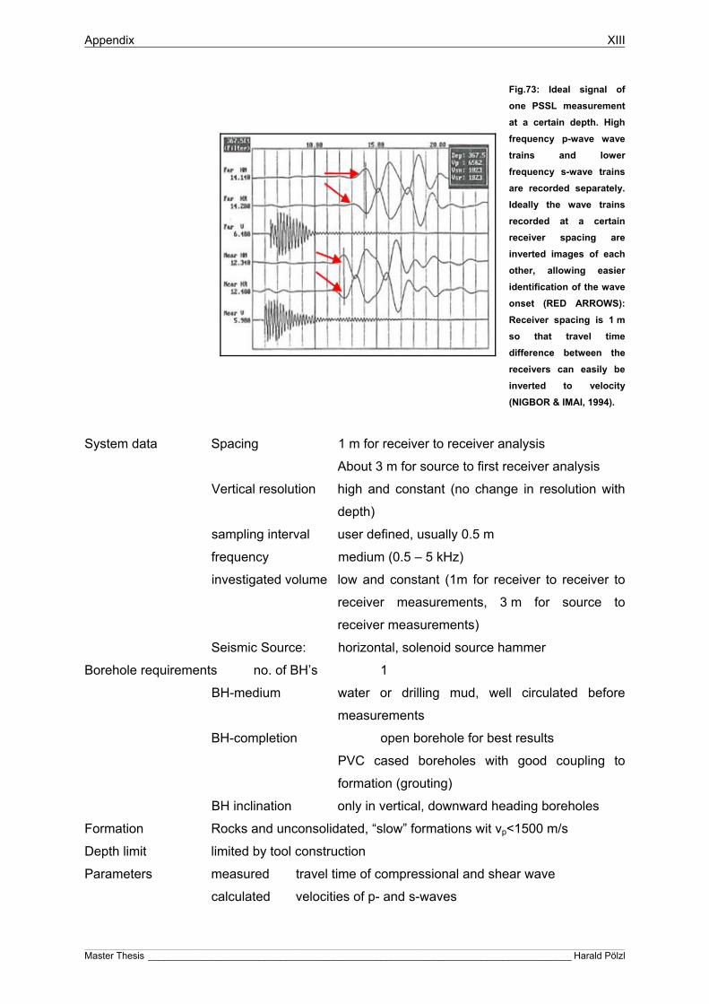
Appendix XIII
____________________________________________________________________________________________________________________________________________________________________________________________________________
Master Thesis ________________________________________________________________________________ Harald Pölzl
Fig.73: Ideal signal of
one PSSL measurement
at a certain depth. High
frequency p-wave wave
trains and lower
frequency s-wave trains
are recorded separately.
Ideally the wave trains
recorded at a certain
receiver spacing are
inverted images of each
other, allowing easier
identification of the wave
onset (RED ARROWS):
Receiver spacing is 1 m
so that travel time
difference between the
receivers can easily be
inverted to velocity
(NIGBOR & IMAI, 1994).
System data Spacing 1 m for receiver to receiver analysis
About 3 m for source to first receiver analysis
Vertical resolution high and constant (no change in resolution with
depth)
sampling interval user defined, usually 0.5 m
frequency medium (0.5 – 5 kHz)
investigated volume low and constant (1m for receiver to receiver to
receiver measurements, 3 m for source to
receiver measurements)
Seismic Source: horizontal, solenoid source hammer
Borehole requirements no. of BH’s 1
BH-medium water or drilling mud, well circulated before
measurements
BH-completion open borehole for best results
PVC cased boreholes with good coupling to
formation (grouting)
BH inclination only in vertical, downward heading boreholes
Formation Rocks and unconsolidated, “slow” formations wit vp<1500 m/s
Depth limit limited by tool construction
Parameters measured travel time of compressional and shear wave
calculated velocities of p- and s-waves
Appendix XIV
____________________________________________________________________________________________________________________________________________________________________________________________________________
Master Thesis ________________________________________________________________________________ Harald Pölzl
Measuring progress low to medium due to stationary measurements every 0.5 m (or other
user defined sampling interval).
Comment Aspects that should be taken into account for the use of PSSL:
- Source to first receiver measurements are affected by an internal
source delay that can be easily verified, but which can change
within a logging section due to deterioration or damaging of source
springs.
- Measurements in PVC casings are possible, but casing should be
carefully grouted at least 48 hours before measurements, to
provide good coupling to the formation. Voids in the grouting cause
problems with de data.
- Measurements in steel casing do not provide sufficient results.
- Highly fractured rocks cause problems due to attenuation, complex
refraction and reflection of wave energy. First arrival picking might
be impossible or lead to unreliable results.
- Highly alteration of the borehole wall (f.ex due to repeated rod
movement) causes problems.
- Mispicking of non corresponding phases can cause errors in the
range of about 5 – 50 ms especially in unconsolidated sediments.
References on PSSL
ELLIS E.V., SINGER J.M., 2007, Well Logging for Earth Scientists. 2nd Edition, Springer Verlag,
Dortrecht, 2007, p.247-322.
NIGBOR, R.L. and IMAI, T., 1994. The Supension P-S Velocity Logging Method. IN: Geophysical
Characterization of Sites, Volume prepared by ISSMFE Technical Committee #10 for XIII ICSMFE,
1994, New Delhi, India. Edited by Richard D. WOODS, International Science Publisher, New York,
1994, p.57-61.
DIEHL., J.G., MARTIN, A.J. and STELLER, R.A., 2006. Twenty year retrospective on the OYO P-S-
suspension logger. Proceedings of the 8th U.S.National Conference on Earthquake Engineering, April
18-22, 2006, San Francisco, California, USA, Paper No. 319.
INAZAKI, T. Relationship between s-wave velocities and geotechnical properties of alluvial sediments,
2006. Public Works Research Institute, Tsukuba, Japan, 2006.

Appendix XV
____________________________________________________________________________________________________________________________________________________________________________________________________________
Master Thesis ________________________________________________________________________________ Harald Pölzl
Gamma Gamma Density Log
Method description Gamma-Gamma-Density Logging (GGD) uses artificial sources of
radiation (usually 137Cs or 60Co) to measure interaction between
emitted radiation and rock formations in boreholes. The dominant
interaction process is the Compton effect. Proper calibration of the tool
allows measurement of electron density using a GGD-tool comprising a
Gamma radiation source, 1 or more detectors (preferred 2 to overcome
artefacts caused by wall roughness, mud cakes or break outs) and a
positioning system to press the tool against the wall (usually a
mechanical arm that is capable of measuring the borehole caliper). A
lead isolation prevents direct radiation from source to receiver. The
bulk density is calculated from the electron density.
GGD measurements are mainly used for porosity estimations
(petroleum industry), for density measurements as input parameter for
mechanical property derivation (combined with velocity measurements)
and as a support in lithological classification.
Fig.74: GGD tool and its use in a
borehole (ELLIS, 2007).
System data Vertical resolution high and constant
sampling interval user defined (usually around 0.1 m)
investigated volume low and +/- constant (radiation penetration depth
might vary for different materials)
Radiation Source: 137Cs or 60Co
Appendix XVI
____________________________________________________________________________________________________________________________________________________________________________________________________________
Master Thesis ________________________________________________________________________________ Harald Pölzl
Borehole requirements no. of BH’s at least 1
BH-medium fluid filled (no extremely heavy weight muds)
In dry holes absolute density values are
unreliable, but relative changes can still be
interpreted (lithological changes, fractured zones)
BH-completion open borehole for best results
In cased water wells GGD can be run to check
material
in the annular space.
BH diameter dependant on the tool (especially the positioning
system), usually in the range between 70 –
220 mm
BH inclination best results in vertical holes.
In high quality boreholes (f.ex. in granites)
inclinations up to 25° can be measured without
significant data quality loss. Theoretically if wall
contact can be provided higher inclinations are
possible, but risk of tool loss or tool damage is
increasing with higher inclinations.
Formation Rocks and soils
Depth limit limited by tool construction
Parameters measured Formation electron density and borehole caliper
calculated Formation Bulk density
Measuring progress medium to high
Comment Aspects that should be taken into account for the use of GGD:
- Handling radioactive materials needs special training and
surveillance (dosimeter).
- Radioactive tools need more time for international transport and its
organisation (special papers for customs, …).
References on GGD
ELLIS E.V., SINGER J.M., 2007, Well Logging for Earth Scientists. 2nd Edition, Springer Verlag,
Dortrecht, 2007, p.247-322.

Appendix XVII
____________________________________________________________________________________________________________________________________________________________________________________________________________
Master Thesis ________________________________________________________________________________ Harald Pölzl
Downhole Seismic
Method description Downhole seismic measurements (Vertical Seimic Profiles-VSP, well
velocity surveys) record seismic signals created by surficial sources
with geophones or hydrophones at different depths in a well.
BOYER&MARY, 1997 describe the VSP as an acoustic log at seismic
frequencies.
Fig.75: Principle of downhole seismic
measurements in a layered medium.
(http://seismo.geology.upatras.gr).
Seismic signals produced by a surficial
source are recorded by receivers (geo-
or hydrophones) in a well.
For the measurements the receivers (1 geophone or an array) are
lowered in the borehole to a certain depth and clamped to the borehole
wall to increase signal to noise ratio and to avoid receiver movement.
After source activation and signal recording receivers are unclamped
and moved to the next depth. The use of a reference geophone on the
surface provides measurements significance.
To obtain velocity data first arrivals are picked. For the fact that
normally source and receiver are not on the same vertical, corrections
are necessary. ANDERSON et al., 2003 recommend the use of two
opposite polarized shear wave records for shear wave travel time
measurements. Traveltime plots versus depth allow the differentiation
of layers with approximately constant velocities.
The downhole wavefield is composed by downgoing body waves
(direct arrivals from the source or reflected waves from markers above
the receiver), upgoing body waves (primary or multiple reflected p- and
s-waves) and Stoneley waves (guided interface modes linked to well
and fluid).

Appendix XVIII
____________________________________________________________________________________________________________________________________________________________________________________________________________
Master Thesis ________________________________________________________________________________ Harald Pölzl
Fig.76: Downhole data
example
(BOYER&MARY, 1997).
The wave field is
composed of
downgoing and
upgoing bodywaves
and tube waves (TW1, 3
and 6 are downgoing;
TW 2, 4 and 5 are
upgoing).
System data Spacing user defined, usually in the range between 1 and
5 m
Vertical resolution medium to low, dependant on the receiver
spacing
sampling interval user defined (usually from 1 m to 10 m)
frequency medium to low, source dependant
investigated volume high, lateral investigation distance is about half
the well head-source offset, but limited by the
fact that the incident angle must be beneath 30-
35° to markers.
Seismic Source: Onshore: sledge hammers, low charge
explosives, dropped weights or offshore sources
in mudpits
Offshore: Airguns
Borehole requirements no. of BH’s 1
BH-medium dry or fluid filled holes
BH-completion preferred in cased holes (PVC), accurate
coupling of the receivers to the formation must be
possible (grouting)
BH diameter equipement dependant

Appendix XIX
____________________________________________________________________________________________________________________________________________________________________________________________________________
Master Thesis ________________________________________________________________________________ Harald Pölzl
BH inclination possible in vertical, inclined and deviated wells
Formation Rocks and soils
Depth limit limited by tool construction and source range
Parameters measured travel time of compressional and shear wave
calculated velocities of p- and s-waves as a function of depth
Measuring progress medium to high, equipment dependant
Comment Aspects that should be taken into account for the use of downhole
seismics:
- Equipment cables in the borehole should be slackened during
recording to avoid cable waves.
- Ideally measurement points lie beneath markers to avoid
interference between downgoing and a reflected upgoing waves.
- Normally measurements are performed downwards.
Remeasurement of some points while raising the tool provides
repeatability of the measurements. Stacking of (usually up to 5)
consecutive shots increases the signal to noise ratio significantly.
- The long travel paths lead to wave energy loss due to attenuation,
to reflections and to mode conversions (f.ex. in shallow fractures).
- Increasing source receiver spacing increases the influence of
attenuation (especially of the higher frequencies). On the one hand
this is a problem for the measurements (especially for manual first
arrival picking) on the other hand downhole seismics can be used
for macro attenuation analysis using for example “Spectral ratio
method” or “rise time method for VSP recorded with impulsive
sources”.
- Derived velocity functions are estimated via linear trend lines.
Deviations away from the best fit line are result of small scale
variations in material velocity and errors deriving from source-
receiver geometry assumptions, picking insecurities and refraction
effects.
- The use of triaxial geophones allows picking of vertical p-wave
components arrivals and the two horizontal shear wave
components. This can be used for rough anisotropy estimations.
- Triaxial geophones should be oriented parallel to the axis of
excitation at the surface to insure maximal signal amplitude in the
records (f.ex. Geostuff BHG-3 system). Orientation also avoids
errors in travel time caused by incorrect phase of first arrival picks.

Appendix XX
____________________________________________________________________________________________________________________________________________________________________________________________________________
Master Thesis ________________________________________________________________________________ Harald Pölzl
- Tube waves can be used to identify fractured and permeable
zones.
- Verticality of the hole is mostly assumed, although vertical drilled
holes can show significant inclinations especially with increasing
borehole depth. Additional borehole deviation measurements can
provide data for more exact surface to borehole data processing. In
inclined or deviated wells borehole deviation must be measured.
Another possibility to remove or reduce inclination effects is the use
of two receivers and the calculation of interval velocities.
References
CHEN S.T., ZIMMERMANN L.J., TUGNAIT J.K., 1990, Subsurface imaging using reversed vertical
seismic profiling and crosshole tomographic methods. Geophysics, Vo.55, No.11, November 1990,
p.1478-1487.
BOYER, S., MARI, J.-L., 1997, Oil and Gas Exploration Techniques: Seismic Surveying and Well
Logging. Editions Technip, Paris, 1997
Crosshole Seismic
Method description For crosshole seismic measurements sources and receivers are
installed in certain depth positions in separated boreholes (“source-
“and “receiver hole”).
Fig.77: Principal of
crosshole surveys.
Source and receiver
are positioned in
separated holes. For
“classic” crosshole
seismic source and
receiver are usually
positioned in the
same depth (red
arrow)
The source is activated in several positions in the source hole and the
emerged waves are recorded by a receiver or a receiver array in the

Appendix XXI
____________________________________________________________________________________________________________________________________________________________________________________________________________
Master Thesis ________________________________________________________________________________ Harald Pölzl
receiver hole. The crosshole wavefield is mainly composed by direct p-
waves from source hole to receiver, p-waves emitted from the source
and reflected from the surface, p-waves from the source travelling to
the bottom/ground of the receiver hole and converted into a tube wave
going downward/upward to the receivers, p-waves reflected from
structures between the holes and multiple reflected modes of the
former generated tube waves. Velocity can be calculated from manual
picking of first arrivals or by tomographic inversion. Source receiver
geometries can be varied. Simplest geometry is one source and one
receiver installed at the same depth. For tomographic measurements
receiver arrays are used to provide better ray path coverage
Stacking increases signal to noise ratio. Borehole deviation must be
measured to determine exact distances for velocity calculations.
System data Spacing user defined
Lateral resolution medium to high
Vertical resolution medium to high
sampling interval user defined
frequency medium to low, source dependant
investigated volume high, dependant on the hole distance
Seismic Source: low charge explosives, hammer sources, sparker
sources
Borehole requirements no. of BH’s at least 2, preferred 3 or more
BH-medium fluid filled holes, dry holes
BH-completion cased and cemented holes (PVC or aluminium)
BH diameter equipment dependant
BH inclination possible in vertical, inclined and deviated wells
Formation Soils and rocks
Depth limit limited by tool construction
Parameters measured travel time of compressional and shear wave
calculated velocities of p- and s-waves
Measuring progress low to medium
Comment Aspects that should be taken into account for the use of CH:
- Potential sources of error for velocity estimation are recognition and
subsequent correct picking of arrival times, source trigger timing,
difficult borehole conditions and geometric effects.

Appendix XXII
____________________________________________________________________________________________________________________________________________________________________________________________________________
Master Thesis ________________________________________________________________________________ Harald Pölzl
- Low velocity layers can cause problems in shear wave velocity
estimation, because the first arrival tends to be a refraction from the
adjacent higher velocity layer.
- Optimal data quality is provided by performing separate tests for p-
and s-wave measurements.
References
ANDERSON N., CHEN G., KOCIU S., LUNA R., THITIMAKORN T., MALOVICHO A., MALOVICHKO
D., SHYLAKOV D., 2003, Final report RDT 03-006, Vertical Shear-Wave Velocity Profiles Generated
From Spectral Analysis Of Surface Waves: Field Examples. Prepared for Missouri Departement of
Transportation, Research, Development and Technology, Jefferson City, Missouri, April 2003.
CHEN S.T., ZIMMERMANN L.J., TUGNAIT J.K., 1990, Subsurface imaging using reversed vertical
seismic profiling and crosshole tomographic methods. Geophysics, Vo.55, No.11, November 1990,
p.1478-1487.
ANGIONI T., RECHTIEN R.D., CARDIMONA S.J., LUNA R., 2003, Crosshole seismic tomography
and borehole logging for engineering site characterization in Sikeston, MO, USA. Tectonophysics,
368, Elsevier, 2003, p.119-137.

Appendix XXIII
____________________________________________________________________________________________________________________________________________________________________________________________________________
Master Thesis ________________________________________________________________________________ Harald Pölzl
3-Axial and Unconfined Compression Test
Method description Triaxial testing applies a vertical load (σ1) and radial confining pressure
(σ2, σ3) on a cylindrical or a cuboid sample with mechanic pistons or
fluids. Compression can be realized as well as extension. Different
combinations of stress relations allow testing under different
conditions. The conventional triaxial test shows two equal stresses
(σ1>σ2=σ3 or σ1=σ2>σ3). The true triaxial test is performed in a more
general stress state (σ1≥σ2≥σ3). Unconfined compression tests are
performed applying only axial stress without confining pressures.
Fig.78: Different stress conditions realized
in triaxial experiments. A: only fluid
pressure. B: piston pressure
C,D: Combination of pistons and fluid
pressures (MOGI, 2009)
Usually the specimen is jacketed with rubber and connected with a
hydraulic pressure machine. Pressure measurements are realized via
Bourdon Gauge and a load cell over electrical resistance strain gauge.
According to the geometry an internal and an external method can be
differentiated.

Appendix XXIV
____________________________________________________________________________________________________________________________________________________________________________________________________________
Master Thesis ________________________________________________________________________________ Harald Pölzl
Fig.79: Internal
and External
methods (MOGI,
2009)
The triaxial test can be performed under drained and under undrained
conditions. Fluid conditions are controlled by a valve system.
Fig.80: Triaxial Cell and its
main compinents.
Accordint to the different conditions of testing the following triaxial test
methods can be sifferentiated:
- Consolidated and drained (CD- or S-) compression or extension
test
- Consolidated and undrained (CU- or R-) compression or extension
test
- Unconsolidated and undrained (UU- or Q-) compression or
extension test
The Unconfined compression test is the simplest form of a triaxial
testing. The sample is loaded axial without confining pressure until
failure. The pressure at failure is the Unconfined Compression
strength, which is a widely used parameter in geo-engineering (UCS).
System data aspect Ratio usually 2:1
investigated volume low to medium

Appendix XXV
____________________________________________________________________________________________________________________________________________________________________________________________________________
Master Thesis ________________________________________________________________________________ Harald Pölzl
Borehole requirements no. of BH’s at least 1 hole with coring for sample
material
Formation Rocks and soils
Depth limit limited by depth of the sampling borehole
Parameters measured fracture/failure stress, yield stress, ductility
fracture angle between shear fault plane and σ1-axis
Fig.81: Stress.strain
curve measured in
triaxial experiments and
derived parameters.
(MOGI, 2009).
calculated moduli, cohesion, internal angle of friction, shear trength
Measuring progress low (coring-transportation to lab-sample preparation-test)
Comment Aspects that should be taken into account for the use of triaxial tests
- A pressure effect at the end of the specimens leads to a decreasing
strength with increasing confining pressure. Conventional tests with
small cylindrical samples are accompanied by stress concentration
and a clamping effect at the end part of the specimen.
- In drained measurements the loading rate plays an essential role. If
loading rate is too high the pore pressure increases and the elastic
constants measured are approaching the ones measured under
undrained conditions. According to this the undrained test allow
application of higher stress rates.
- Friction between sample and pistons lead to a barrel form of the
sample during testing. This effect can be minored by aspect ratios
of at least 2.
- Friction occurring at moving pistons can produce hysteresis effect
during unloading.
References
CHARLEZ, A.P., 1991, Rock Mechanics, Volume 1, Theoretical Fundamentals. Editions Technip,
Paris, 1991, p. 159-174.
HUNT, R.E., 2005. Geotechnical engineering investigation handbook. Tayor&Francis, CRC, Boca
Raton, 2005, 1066 pages.

Appendix XXVI
____________________________________________________________________________________________________________________________________________________________________________________________________________
Master Thesis ________________________________________________________________________________ Harald Pölzl
MOGI, K., 2007, Experimental Rock Mechanics. In: Kwasniewski, A.M. (editor in chief), 2007,
geomechanics Research Series Vol. 3. Taylor&Francis Group, London, UK, 2007, p. 3-193.
ZHANG, L., 2005. Engineering properties of rocks. Elsevier geo-engineering book series, Vol. 4,
Elsevier, Amsterdam, 2005, 290 p.
Piezo-Element testing (transmission and Bender elements)
Method description A cylindrical sample is fixed between two ultrasonic, usually piezo-
transducers. Piezoceramic elements can be mechanically stressed by
an applied voltage or can produce an electrical charge when stressed
by an applied force. For traveltime measurements the sample of known
length (travel path) is positioned between a transmitting and a
receiving element. For the fact that “normal” piezoceramic elements
are not adequate to measure shear wave velocity in soil samples
(weak s-wave directivity, poor coupling, high operating frequencies)
bender elements have been developed. Bender elements are thin, two
layered plates consisting of two conductive outer electrodes, two
piezoceramic sheets and a conductive metal shim at the centre. Series
and parallel elements have to be distinguished. Parallel elements show
twice the displacement of the series element for the same applied
voltage and are used as sources, whereas series elements are used
as receivers.
Fig.82: (a) schematic
representation of a bender
element, (b) series type
element and (c) parallel
element
(LEE&SANTAMARINA, 2005).

Appendix XXVII
____________________________________________________________________________________________________________________________________________________________________________________________________________
Master Thesis ________________________________________________________________________________ Harald Pölzl
Traveltime determination can be done in different ways:
- First arrival picking
- Determination between characteristic points
- Cross correlation of input and output signal
- Determination of group traveltimes for a range of frequencies
- Use of second (or third) arrivals (reflections)
Fig.83: Principle setup for laboratory
velocity measurements using piezo-
elements. (http://www.bgu.ac.il/geol/rockmec
h/lab/ultrasonic.html)
System data aspect Ratio: different geometries possible
frequency high, > 6 kHz
investigated volume low
Borehole requirements: no. of BH’s at least 1 hole with coring for sample material
Formation Rocks and soils (bender elements)
Depth limit limited by borehole depth
Parameters measured p- and s-wave travel time
calculated wave velocity
Measuring progress low (coring-transportation to lab-sample preparation-test)
Comment Aspects that should be taken into account for the use of Piezoceramic element
tests.
- Bender elements involve some sources of travel time errors like
interference of p- and s-wave arrivals, near field effects, reflections
at sample boundaries resulting in non directive wave travel paths
through the sample, rotational compliance of the bender to cap
connection, disturbances at the sample-bender-interface, imperfect
alignment of the benders and the fact that for given geometries the
source cannot be seen as a point source. This error sources are
still subject to research.
- ARULNATHAN et al., 1998 mention a high dependence of travel
time errors on bender length to wavelength ratio, on the method of
Appendix XXVIII
____________________________________________________________________________________________________________________________________________________________________________________________________________
Master Thesis ________________________________________________________________________________ Harald Pölzl
traveltime determination and on the relative stiffness of sample and
bender element.
- Electromagnetic coupling can lead to “crosstalk”, an early signal
component that is quasi-simultaneous with the input signal.
References
ARULNATHAN, R., BOULANGER, R.W. and RIEMER, M., 1998. Analysis of Bender Element Tests.
Geotechnical Testing Journal, GTJODJ, Vol. 21, No. 2, 1998, p. 120-131.
LEE, J.-S. and SANTAMARINA, C., 2005. Bender Elements: Performance and Signal Interpretation.
Journal of Geotechnical and geoenvironmental Engineering, ASCE, September 2005, p. 1063-1070.