Correlation analysis 1: Canonical correlationanalysis

Ryan TibshiraniData Mining: 36-462/36-662

February 14 2013

1

Review: correlation

Given two random variables X,Y ∈ R, the (Pearson) correlationbetween X and Y is defined as

Cor(X,Y ) =Cov(X,Y )√

Var(X)√

Var(Y )

Recall that

Cov(X,Y ) = E[(X − E[X])(Y − E[Y ])

]and

Var(X) = E[(X − E[X])2

]= Cov(X,X)

This measures a linear association between X,Y . Properties:

I −1 ≤ Cor(X,Y ) ≤ 1

I X,Y independent ⇒ Cor(X,Y ) = 0 (Homework 2)

I Cor(X,Y ) = 0 6⇒ X,Y independent (Homework 2)

More on this later ...2

Review: sample correlation

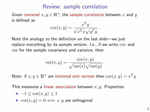
Given centered x, y ∈ Rn, the sample correlation between x and yis defined as

cor(x, y) =xT y√

xTx√yT y

.

Note the analogy to the definition on the last slide—we justreplace everything by its sample version. I.e., if we write cov andvar for the sample covariance and variance, then

cor(x, y) =cov(x, y)√

var(x)√var(y)

.

Note: if x, y ∈ Rn are centered unit vectors then cor(x, y) = xT y

This measures a linear association between x, y. Properties:

I −1 ≤ cor(x, y) ≤ 1

I cor(x, y) = 0 ⇐⇒ x, y are orthogonal

3

Canonical correlation analysis

Principal component analysis attempts to answer the question:“which directions account for much of the observed variance in adata set?” Given a centered matrix X ∈ Rn×p, we first find thedirection v1 ∈ Rp to maximize the sample variance of Xv:

v1 = argmax‖v‖2=1

var(Xv)

Canonical correlation analysis is similar but instead attempts toanswer: “which directions account for much of the covariancebetween two data sets?” Now we are given two centered matricesX ∈ Rn×p, Y ∈ Rn×q, and we seek the two directions α1 ∈ Rp,β1 ∈ Rq that maximize the sample covariance of Xα and Y β:

α1, β1 = argmax‖Xα‖2=1, ‖Y β‖2=1

cov(Xα, Y β)

Subject to the constraints, this is equivalent to maximizingcor(Xα, Y β). (Why?)

4

Canonical directions and variates

The first canonical directions α1 ∈ Rp, β1 ∈ Rq are given by

α1, β1 = argmax‖Xα‖2=1, ‖Y β‖2=1

(Xα)T (Y β)

Vectors Xα1, Y β1 ∈ Rn are called the first canonical variates, andρ1 = (Xα1)

T (Y β1) ∈ R is called the first canonical correlation

Given the first k − 1 directions, the kth canonical directionsαk ∈ Rp, βk ∈ Rq are defined as

αk, βk = argmax‖Xα‖2=1, ‖Y β‖2=1

(Xα)T (Xαj)=0, j=1,...k−1(Y β)T (Y βj)=0, j=1,...k−1

(Xα)T (Y β)

Vectors Xαk, Y βk ∈ Rn are called the kth canonical variates, andρk = (Xαk)

T (Y βk) ∈ R is called the kth canonical correlation

5

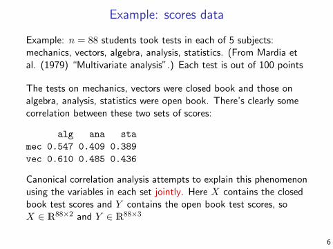
Example: scores data

Example: n = 88 students took tests in each of 5 subjects:mechanics, vectors, algebra, analysis, statistics. (From Mardia etal. (1979) “Multivariate analysis”.) Each test is out of 100 points

The tests on mechanics, vectors were closed book and those onalgebra, analysis, statistics were open book. There’s clearly somecorrelation between these two sets of scores:

alg ana sta

mec 0.547 0.409 0.389

vec 0.610 0.485 0.436

Canonical correlation analysis attempts to explain this phenomenonusing the variables in each set jointly. Here X contains the closedbook test scores and Y contains the open book test scores, soX ∈ R88×2 and Y ∈ R88×3

6

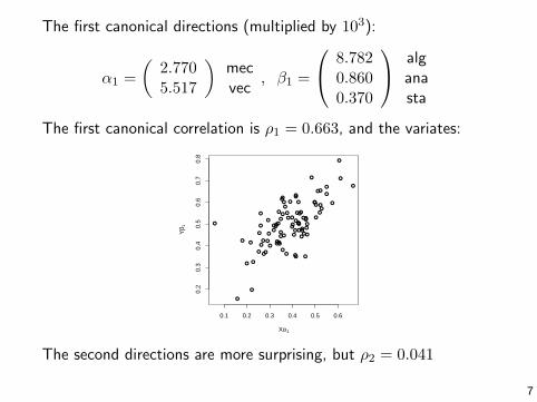
The first canonical directions (multiplied by 103):

α1 =

(2.7705.517

)mecvec

, β1 =

8.7820.8600.370

alganasta

The first canonical correlation is ρ1 = 0.663, and the variates:

●

●

●

●●

●

●●

● ●●●

●

●

●

●

●

●●●

●

●●

●

●

●

●

●

●

● ●

●●

●●

● ●●●●

●

● ●

●

●

●

●

●

●●●

●

●●

●●

●

●

●

●

●

●

●

●

●

●

●

●

●●

●

●

●●

●

●

●

●

●

●

●

●●

●

●

●

●

●

0.1 0.2 0.3 0.4 0.5 0.6

0.2

0.3

0.4

0.5

0.6

0.7

0.8

Xα1

Yβ 1

The second directions are more surprising, but ρ2 = 0.041

7

How many canonical directions are there?

We have X ∈ Rn×p and Y ∈ Rn×q. How many pairs of canonicaldirections (α1, β1), (α2, β2), . . . are there?

We know that any n orthogonal (linearly independent) vectors inRn form a basis for Rn. Therefore there cannot be more than porthogonal vectors of the form Xα, α ∈ Rp, and q orthogonalvectors of the form Y β, β ∈ Rq. (Why?)

Hence there are exactly r = min{p, q} canonical directions(α1, β1), . . . (αr, βr)

1

1This is assuming that n ≥ p and n ≥ q. In general, there are actually onlyr = min{rank(X), rank(Y )} canonical directions

8

Transforming the problem

If A ∈ Rp×p, B ∈ Rq×q are invertible, then computing

α1, β1 = argmax‖XAα‖2=1, ‖Y Bβ‖2=1

(XAα)T (Y Bβ),

is equivalent to the first step of canonical correlation analysis. Inparticular, the first canonical directions are given by α1 = Aα1 andβ1 = Bβ1. The same is also true of further directions

I.e., we can transform our data matrices to be X = XA, Y = Y Bfor any invertible A,B, solve the canonical correlation problemwith X, Y , and then back-transform to get our desired answers

Why would we ever do this? Because there is a transformationA,B that makes the computational problem simpler

9

SpheringFor any symmetric invertible matrix A ∈ Rn×n, there is a matrixA1/2 ∈ Rn×n, called the (symmetric) square root of A, such thatA1/2A1/2 = A

We write the inverse of A1/2 as A−1/2. Note A−1/2AA−1/2 = I.(Why?)

Given centered matrices X ∈ Rn×p and Y ∈ Rn×q,2 we defineVX = XTX ∈ Rp×p and VY = Y TY ∈ Rq×q. Then

X = XV−1/2X ∈ Rn×p and Y = Y V

−1/2Y ∈ Rn×q

are called the sphered versions of X and Y .3 Note that the samplecovariance of X and Y is

cov(X) = I/n and cov(Y ) = I/n

2Here we are assuming that rank(X) = p and rank(Y ) = q3Alternatively, for sphering we would sometimes define VX = (XTX)/n and

VY = (Y TY )/n, so that the transformed sample covariances are exactly I10

Transforming the problem (continued)

As suggested by the previous slide, we will take X = XV−1/2X and

Y = Y V−1/2Y , and we’ll solve the problem

α1, β1 = argmax‖Xα‖2=1, ‖Y β‖2=1

(Xα)T (Y β)

Recall that then α1 = V−1/2X α1 and β1 = V

−1/2Y β1.

So why is this simpler? Note that the constraint says

1 = (Xα)T (Xα) = αTV−1/2X XTXV

−1/2X α = αT α

i.e., ‖α‖2 = 1. Similarly, ‖β‖2 = 1. Hence our problem can berewritten as:

α1, β1 = argmax‖α‖2=1, ‖β‖2=1

αTMβ

where M = XT Y = V−1/2X XTY V

−1/2Y ∈ Rp×q. The same is true

for further directions

11

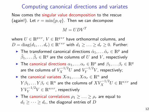
Computing canonical directions and variates

Now comes the singular value decomposition to the rescue(again!). Let r = min{p, q}. Then we can decompose

M = UDV T

where U ∈ Rp×r, V ∈ Rq×r have orthonormal columns, andD = diag(d1, . . . dr) ∈ Rr×r with d1 ≥ . . . ≥ dr ≥ 0. Further:

I The transformed canonical directions α1, . . . αr ∈ Rp andβ1, . . . βr ∈ Rq are the columns of U and V , respectively

I The canonical directions α1, . . . αr ∈ Rp and β1, . . . βr ∈ Rq

are the columns of V−1/2X U and V

−1/2Y V , respectively;

I the canonical variates Xα1, . . . Xαr ∈ Rn and

Y β1, . . . Y βr ∈ Rn are the columns of XV−1/2X U ∈ Rn×r and

Y V−1/2Y V ∈ Rn×r, respectively

I The canonical correlations ρ1 ≥ . . . ≥ ρr are equal tod1 ≥ · · · ≥ dr, the diagonal entries of D

12

Example: olive oil data

Example: n = 572 olive oils, with p = 9 features (the olives dataset from the R package classifly):

1. region2. palmitic3. palmitoleic4. stearic5. oleic6. linoleic7. linolenic8. arachidic9. eicosenoic

Variable 1 takes values in {1, 2, 3}, indicating the region (in Italy)of origin. Variables 2-9 are continuous valued and measure thepercentage composition of 8 different fatty acids

13

We are interested in the correlations between the region of originand the fatty acid measurements. Hence we take X ∈ R572×8 tocontain the fatty acid measurements, and Y ∈ R572×3 to be anindicator matrix, i.e., each row of Y indicates the region with a 1and otherwise has 0s. This might look like:

Y =

1 0 01 0 00 0 10 1 0

. . .

(In this case, canonical correlation analysis actually does the exactsame thing as linear discriminant analysis, an important tool thatwe will learn later for classification)

14

The first two canonical X variates, with the points colored byregion:

●

●

●

●●●

●

●

●

●

●●

● ●

●

●

●

●

●

●●●

●

●

●

●

●

●

●●●

●

●●●●

●

●

●●

● ●●●

●

●●

●●

●

●●

●

●

●

●

●

●

●

●

●

●

●

●

●

●

●●

●●●● ●

●

●

●●

●

●

●●

●

●

●

●

●

●

●●

●●

●

●●

●

● ●

●

●

●

●

●

●

●●

●

●

●

●

●●

●

●

●

●

●●

●

●●

●

●

●

●●●●●

●

●●●

●

●

●●

●

●

●

● ●●

● ●

●

●

●

●

●●●

●

●

●●

●●

●●

●●

●

●

●

●●

●

●●

●

●

●●

●●

●

●

●●

●

●●

●

●

● ●

●

●

●

●

●●

●

●

●

●●

●

●● ●

●

●●

●

●●

● ●●

●

●

●●

●

●

●

●

●

●●

●

●●

●●

●

●

●

●

●

●

●●

●

●

● ●●

●

●●

●

●

●●

●

●

●

●

●

●

●

●

●

●

●

●

●

●

●

●

●●

●

●

●

●

●●

●

●●

●

●

●

●

●

●

●●

●

●

●●

●

●

●●

●●

●

●

●

●

●

●

●●

●

●

●●●

●

●●

●

●

●

●●

●

●●

●

●

●●

●

●

●

●

●●

●

● ●

●

●●

●●

●

●

●●●

●

●

●●

●

●

●●

●

●

●●

●

●

●●

●●

●

●

●

●●

●

●●

●

●

●

●

●

●

●

●

●

●

●

●

●●●●

●

●

●●●

●

●

●●

●

●

●

●●

●●

●●

●

●

●

●●

●

●●

●●

●●

●●

●

●●●

●

●

●●

●

●●●

●

●

●●

●

●

●

●●●

●●●

●

●

●

●

●

●●

●●

●

●●

●●●

●●

●

●●

●●

●

●

●●

●

●

●●

●

●

●

●

●

●

●

●●

●

●

●

●

●

●●

●

●●

●

●●●

●●

●

●

●

●

●● ●

●

●

●

●●

●

●

●

●

●

●

●

●

●

●

●● ●

●

●

●●

●●●

●

●

●

●

●●● ●

●

●

●●

●

●●●

●

●

●●

●

●

●

●

●●

●

●

●●●

●

●

●

● ●

●●

●●

●

●●

●

●

●

● ●

−0.25 −0.20 −0.15 −0.10

1.20

1.25

1.30

1.35

1.40

First canonical x variate

Sec

ond

cano

nica

l x v

aria

te

●

●

●

Region 1Region 2Region 3

15

Canonical correlation analysis in R

Canonical correlation analysis is implemented by the cancor

function in the base distribution. E.g.,

cc = cancor(x,y)

alpha = cc$xcoef

beta = cc$ycoef

rho = cc$cor

xvars = x %*% alpha

yvars = y %*% beta

16

Recap: canonical correlation analysis

In canonical correlation analysis we are looking for pairs ofdirections, one in each of the feature spaces of two data setsX ∈ Rn×p, Y ∈ Rn×q, to maximize the covariance (or correlation)

We defined the pairs of canonical directions (α1, β1), . . . (αr, βr),where r = min{p, q}, and αj ∈ Rp, βj ∈ Rq. We also defined thepairs of canonical variates (Xα1, Xβ1), . . . (Xαr, Xβr), whereXαj ∈ Rn and Xβj ∈ Rn. Finally, we defined the canonicalcorrelations ρ1, . . . ρr ∈ R

We saw that transforming the problem leads to a simpler form.From this simpler form we can compute the canonical directions,correlations, and variates using the singular value decomposition

17

Next time: measures of correlation

A lot of work has been done, but there’s still a lot of interest

. . .1888 2012

18