applied physics, faculty of applied sciences, TU Delft

Correcton Method for Neutron Transport Calculations with RealTime Flux Estimation

Bachelor thesis

Name: Hennink, AldoStudent Number: 1513222Supervisors: dr. ir. Eduard Hoogenboom, department: PNR

Bart Sjenitzer, MSCStarting Date: September 22, 2011Final Date: March 1, 2012

Not Confidential

Correcton Method for Neutron Transport

Calculations with Real Time Flux Estimation

Hennink, Aldo

March 1, 2012

Abstract

A new self-learning Monte Carlo technique is presented that enhances sourceconvergence in loosely coupled systems. It uses correctons in combination withan estimate of the neutron flux, resulting in a particle flux with little or no spatialvariation. The estimate is obtained in real time, i.e.: during the calculation.Therefore, no prior Monte Carlo simulations or deterministic calculations arenecessary.

The method solves the source convergence problem for several simplifiedsystems of fuel assemblies for which a conventional calculation with neutronsfails.

Contents

1 Introduction 31.1 Setup of this thesis . . . . . . . . . . . . . . . . . . . . . . . . . . 31.2 Acknowledgement . . . . . . . . . . . . . . . . . . . . . . . . . . . 4

2 Introduction to Nuclear Reactor Physics 52.1 Nuclear reactions . . . . . . . . . . . . . . . . . . . . . . . . . . . 52.2 Neutron Transport . . . . . . . . . . . . . . . . . . . . . . . . . . 72.3 Criticality . . . . . . . . . . . . . . . . . . . . . . . . . . . . . . . 8

3 Monte Carlo Method for Neutron Transport and CriticalityCalculations 103.1 Introduction to the Monte Carlo method . . . . . . . . . . . . . . 103.2 Rewriting the neutron transport equation . . . . . . . . . . . . . 113.3 Source iteration . . . . . . . . . . . . . . . . . . . . . . . . . . . . 143.4 Particle histories . . . . . . . . . . . . . . . . . . . . . . . . . . . 15

3.4.1 Sampling from the kernels . . . . . . . . . . . . . . . . . . 153.4.2 Simulating neutrons . . . . . . . . . . . . . . . . . . . . . 16

3.5 Criticality calculation using the Monte Carlo method . . . . . . . 163.6 The scoring method . . . . . . . . . . . . . . . . . . . . . . . . . 173.7 Standard variance reduction methods . . . . . . . . . . . . . . . . 183.8 Difficulties . . . . . . . . . . . . . . . . . . . . . . . . . . . . . . . 19

4 The Correcton Method 214.1 Introduction and justification . . . . . . . . . . . . . . . . . . . . 214.2 The choice of Υ(~r) . . . . . . . . . . . . . . . . . . . . . . . . . . 23

4.2.1 Limitations . . . . . . . . . . . . . . . . . . . . . . . . . . 234.2.2 Mathematical representation . . . . . . . . . . . . . . . . 24

4.3 Real time flux estimation . . . . . . . . . . . . . . . . . . . . . . 244.4 Estimating the neutron flux from correcton histories . . . . . . . 254.5 Estimating the flux parameters . . . . . . . . . . . . . . . . . . . 26

4.5.1 Choosing ~βi,j,k . . . . . . . . . . . . . . . . . . . . . . . . 264.5.2 Adjusting the Ki,j,k . . . . . . . . . . . . . . . . . . . . . 27

5 Numerical Examples 305.1 System 1: a homogeneous rectangular parallelepiped . . . . . . . 30

5.1.1 Basic criticality calculation with neutrons . . . . . . . . . 305.1.1.1 Estimating the error of the final result . . . . . . 31

5.1.2 Robustness tests for the correcton method . . . . . . . . . 32

1

5.1.2.1 Criticality calculation with correctons for system 1 325.1.2.2 Correctons with a discontinuous Υ(~r) in system 1 335.1.2.3 Correctons with a changing Υ(~r) in system 1 . . 35

5.1.3 Real time flux estimation . . . . . . . . . . . . . . . . . . 395.2 System 2: homogenised, loosely coupled fuel assemblies . . . . . 40

5.2.1 Basic neutron calculation . . . . . . . . . . . . . . . . . . 405.2.2 Real time flux estimation . . . . . . . . . . . . . . . . . . 42

5.2.2.1 Two-dimensional flux estimation . . . . . . . . . 455.2.2.2 Choice of the cell sizes . . . . . . . . . . . . . . . 46

5.3 Other tests . . . . . . . . . . . . . . . . . . . . . . . . . . . . . . 46

6 Conclusion 48

7 Future work 49

A Notes on stochastics 50A.1 Probability and random variables . . . . . . . . . . . . . . . . . . 50A.2 Markov chains and MCMC . . . . . . . . . . . . . . . . . . . . . 51

B Sampling stochastic variables 53B.1 Pseudorandom numbers . . . . . . . . . . . . . . . . . . . . . . . 53B.2 Sampling from a known probability density . . . . . . . . . . . . 54B.3 Sampling an isotropic direction vector . . . . . . . . . . . . . . . 55

C System specifications 56C.1 System 1: simple bar . . . . . . . . . . . . . . . . . . . . . . . . . 56C.2 System 2: fuel assembly # 1 . . . . . . . . . . . . . . . . . . . . . 56

2

Chapter 1

Introduction

In order to analyse engineering problems related to neutron transport, numericalmethods are needed. One of those is the Monte Carlo method, which is basedon approximating a deterministic quantity by performing random experiments.

In a Monte Carlo criticality calculation, one performs an iteration that mustconverge after some amount of cycles. For some physical systems, this does nothappen. Also, accurate estimates of the neutron flux can sometimes be verytime-consuming.

Both of these problems could be solved by the correcton method. Unfortu-nately, an estimate of the neutron flux is often needed in advance. This estimatecan be obtained from another (less extensive) Monte Carlo calculation, or byusing more conventional means.

This thesis explores the possibility of a ‘real time’ neutron flux estimationduring a correcton calculation. That is, the neutron flux estimate is adjustedand refined during the calculation.

This thesis is submitted as a partial fulfilment of the bachelor of physicseducation program of the technical university of Delft.

1.1 Setup of this thesis

This thesis should be readable to anyone with a Bachelor’s degree in physics,while at the same time containing sufficient new or advanced material to keepphysicists in the relevant field interested. To facilitate this, two introductorychapters have been added.

Chapter 2 deals with some basic, essential results from nuclear reactorphysics. Chapter 3 (especially sections 3.1 through 3.7) introduces the generalconcept of the Monte Carlo method, its applicability to nuclear calculations andsome of the standard variance reduction methods, without containing any pre-viously unknown material. Anyone already familiar with parts of it can simplyskim through the sections he or she already knows.

Appendix A contains a formal setup of probability theory and Markov chains,which may be new to some.

3

When introducing the Monte Carlo method in chapter 3, it would have beeneasiest to simply start with a particle perspective of neutron transport. Thatway, simulating neutrons would instantly seem intuitive and the mathematicsis almost unnecessary. (This is done in Hoogenboom et. al. [1].)

Instead, the neutron transport equation and the concept of reaction ratedensities from chapter 2 are taken as axioms from which a new formulation ofthe neutron transport equation can be derived. Only then is the validity of theMonte Carlo method for estimating quantities demonstrated.

There are two principle reasons for this choice of presenting the material.First, chapter 3 is mostly aimed at physicist who are already quite familiarwith the neutron transport equation, but have no experience in Monte Carlocalculations. Perhaps more importantly, the intuitive understanding of simu-lated neutrons does not apply to the simulation technique using correctons thatis introduced in chapter 4. The slightly more abstract treatment in chapter 3should make the validity of the correcton method obvious at first sight.

1.2 Acknowledgement

Ending on a more personal note, I would like to thank Bart Sjenitzer for lettingme use his omniscience in the field of Monte Carlo methods in nuclear computingand introducing me to the world of Fortran, Linux, clusters and really justcomputers in general. My gratitude also goes out to the folks at R3, TU Delftand PNR in particular, for making my short stay at their department fun.

4

Chapter 2

Introduction to NuclearReactor Physics

2.1 Nuclear reactions

If an atomic nucleus collides with another nucleus or a subatomic particle, itmight produce particles that are different from the initial particles. Such anevent is referred to as a nuclear reaction. Compared to some charged sub-atomic particles, neutrons can interact with nuclei relatively easily, since theyare not repulsed by the positive charge of the nucleus or the negative charge ofthe electrons. Here the focus of the discussion will lie on the different types ofinteraction neutrons can have with nuclei.

(Nuclear) fission is a nuclear reaction in which a large nucleus splits intosmaller parts. This is accompanied by a (large) release of energy and the pro-duction of subatomic particles, such as neutrons and photons. In the event ofneutron capture, the neutron will be assimilated by the nucleus to form aheavier nucleus. Sometimes the heavier nucleus is unstable, in which case it willdecay.

Fission and capture are both examples of absorption, meaning that theneutron seizes to exist as an individual particle. Conversely, in a scatteringreaction the neutron remains an unbound particle, but it is forced to deviatefrom a straight path by the nucleus. One can make a distinction between elasticand inelastic scattering1, based on whether the kinetic energy of the neutron isconserved. ([2], 12-16)

The number of neutrons in any macroscopic material is too large to keeptrack of the individual particles. Therefore, statistics are used to describe thebehaviour of all neutrons combined. To quantify the probability of certainnuclear interactions, consider the following scenario.

A beam of neutrons with the same speed, energy and direction has a uniformintensity (I) and is incident normally upon the surface of a plane. On the plane,a constant number of nuclei per area (NA) are located. Define the reactionrate R〈j〉 as the amount of nuclear reactions of type 〈j〉 that take place per

1Actually one might argue that elastic scattering is not a nuclear reaction, since the noneof the particles changes. [3]

5

unit of time per area. Since the nuclei are all on the same plane, they cannot‘shield’ each other from being hit by a neutron. Therefore R〈j〉 will simplybe proportional to I and NA. The constant of proportionality is called themicroscopic cross section for reaction type 〈j〉, denoted by σ〈j〉:

R〈j〉 = σ〈j〉INA.

Obviously, the total probability of a nuclear reaction occurring is the sum overall individual probabilities of a specific reaction. Therefore, the cross sectioncorresponding to any nuclear reaction equals the sum over all individual micro-scopic cross sections. This quantity is referred to as the total microscopic crosssection, denoted by σT .

The concept of cross sections can be extended to three dimensions by consid-ering an incident beam of neutrons on a three-dimensional object. Part of theneutrons will collide with the first nuclei, whilst others will travel deeper intothe material. Suppose x is the distance the neutron beam has travelled in thematerial. Then the intensity I of the beam is a function of x. The probability ofcolliding with a nucleus at any point does not depend on the amount of nucleithat have already been passed, so an exponential relationship between I and xis to be expected.

The amount of neutrons that react in the region between x and x + dx isσT IN , where N is the number of nuclei per unit volume. This implies that

dI(x) = −σTNI(x)dx. (2.1)

Solving Eq. (2.1) and setting I(x = 0) = I0 leads to

I = I(x) = I0 exp [−NσTx] .

The macroscopic cross section corresponding to a nuclear reaction oftype 〈j〉, denoted by Σ〈j〉, is now defined as

Σ〈j〉 ≡ Nσ〈j〉. (2.2)

If a material consists of more than one type of material, the effective crosssection is the weighted average of the cross sections of the different materials.

Note that Eq. (2.1) can be rewritten to find the relative decrease of intensityover a distance dx: (

dII

)dx

= −ΣT .

This means that ΣT can be interpreted as the probability per unit length thata neutron will collide with a nucleus. The probability that a neutron will travela distance d without engaging in a nuclear reaction is therefore just

P [no interaction after travelling a distance d] = exp (−ΣT d) .

The probability density function for the distance travelled before undergoing areaction is

p(d) = ΣT exp (−ΣT d) , d > 0 (2.3)

and the average distance travelled before colliding is E [d] = 1/ΣT . ([2], 16-22)

6

2.2 Neutron Transport

The neutron density N is defined by the relation

N(~r, t)d3r ≡ expected number of neutrons in volume d3r at ~r at time t.

This does not take into account the fact that neutrons are discrete particles.Instead, the neutron density is, in general, a continuous function of position.Also, the statistical nature of the problem at hand is ignored. In the followingdiscussion, the neutron density is assumed to be a deterministic function. Inreality, however, it is a stochastic variable. The goal in neutron transport theoryis to find the neutron density at any given position and time. ([2], 105)

Suppose a neutron has a (scalar) speed v. Since Σ〈j〉 is the probability theneutron will engage in a reaction of type 〈j〉 with a nucleus per unit length theneutron travels, the frequency at which a single neutron has such a reactionis vΣT 〈j〉. (This is also called the reaction frequency.) The reaction ratedensity F is the reaction frequency multiplied by the neutron density:

F〈j〉(~r, t) ≡ vΣ〈j〉N(~r, t). (2.4)

F〈j〉(~r, t)d3r is the total frequency at which interactions of type 〈j〉 are occurring

at ~r in volume d3r at time t. ([2], 21, 105)Apparently, the reaction rate depends on the product vN(~r, t). In fact, this

quantity has a name of its own: the (scalar) neutron flux, defined by

φ(~r, t) ≡ vN(~r, t). (2.5)

The name is a bit misleading, since it is entirely different from the usual ‘fluxes’in electromagnetics or fluid mechanics. This flux is a scalar quantity and doesn’tsay anything about the direction in which the neutrons are moving.

The information about the direction of the neutron flow is contained in the(unit) direction vector Ω. Instead of using the neutron speed, it is custom-ary to specify the energy E, which relates to the speed in the classical way. Bydistinguishing between neutrons with different energy and direction, one can de-compose the neutron density into the angular neutron density n(~r, t, E, Ω).2

The interpretation is that n(~r, t, E, Ω)d3rdEdΩ is the number of neutrons ina volume d3r, in an energy range dE and in a solid angle dΩ at ~r, E and Ωrespectively.

A systematic way to derive the equation that describes the angular neutrondensity is to work out the balance equation for a volume of arbitrary shape.Since this equation is valid for any arbitrary volume V in space, the usualargument ∫

Vf(~r) = 0⇒ f(~r) = 0

can be used to derive a differential equation for the neutron density at any point.All this is done in Duderstadt et al. ([2], 111-114). Here only the result is

2It suffices not to consider the complete quantum mechanical state (which would, amongstothers, include spin), but instead to treat the neutrons as classical particles.

7

given, with some explanation of where the terms come from.

∂n

∂t= − vΩ · ∇n(~r,E, Ω, t)︸ ︷︷ ︸

[1]

− vΣTn(~r,E, Ω, t)︸ ︷︷ ︸[2]

+

∫(Ω′,E′)∈(<4π>,R+)

v′Σs(E′ → E, Ω′ → Ω)n(~r,E′, Ω′, t) d(Ω′, E′)

︸ ︷︷ ︸[3]

+ S(~r,E, Ω, t)︸ ︷︷ ︸[4]

(2.6)

The terms represent respectively:

1. neutrons entering and leaving the point in space due to the neutron flux;

2. neutrons with E, Ω entering a collision at ~r (they change their directionand/or energy and thus no longer contribute to n(~r,E, Ω, t));

3. inscattering: neutrons that have a collision at ~r and change their di-rection and energy to Ω and E. Here Σs(E

′ → E, Ω′ → Ω) representsthe cross section that corresponds to the event that a neutron with Ω′, E′

scatters to Ω, E;

4. the source term. It represents all neutrons that come to life at time t andposition ~r with energy E and direction Ω. This includes both neutronsthat are created in a fission reaction and neutrons that are emitted by anexternal source.

Not surprisingly, Eq. (2.6) is known as the neutron transport equation.It is reminiscent of the Boltzmann equation. Unfortunately, it usually cannotbe solved analytically, so simplifications or numerical methods are necessary.

2.3 Criticality

In a fission reaction, new neutrons are created. In turn, some of these neutronsmay engage in a fission reaction, to create more neutrons. This way, a chainreaction can occur. If a neutron generates, on average, more than one newneutron, the total amount of neutrons will increase. If a neutron creates lessthen one new neutron on average, the chain reaction will gradually die out. Theformer case is referred to as supercritical, while the latter is subcritical. Asystem is critical if the number of neutrons remains the same.

To quantify these ideas, the multiplication factor k is introduced:

k ≡ rate of neutron production

rate of neutron loss (due to leakage from the system and absorption)

To perform a direct calculation of k, one could try to approximate the neu-tron transport Eq. (2.6) directly with a standard multigrid method. Needless tosay, this is computationally demanding. (There are seven independent variablesto be taken into account.) Also, the discretisation introduces a bias and themethod may turn out to be unstable.

8

Another approach would be to calculate the expected number of fission neu-trons a neutrons creates in a system. That would include determining

• the probability that a neutron leaks out of the system before absorbing inthe system;

• the probability a neutron will be absorbed in the parts of the system wherefission can occur (the fuel), conditional on being absorbed in the system;

• the probability of fission, conditional on absorption in the fuel;

• the average amount of neutrons produced in a fission reaction.

This is not a trivial task and things get even more complicated when taken intoaccount the fact that neutrons may only fission at low energy, whilst they are‘born’ at high energy. ([2], 74-86)

The numerical approach that will be used here is the source iterationmethod (a variation on the power method) in combination with the MonteCarlo method. This will be explained in sections 3.2 through 3.5.

9

Chapter 3

Monte Carlo Method forNeutron Transport andCriticality Calculations

3.1 Introduction to the Monte Carlo method

In general, the Monte Carlo method uses a stochastic process to solve a deter-ministic problem.1 Basically, it can be summarised as follows. Suppose onewants to approximate a variable x.2 Now the Monte Carlo Method usuallyconsists of the following steps.

1. Find some stochastic process that has realisations θi, with E [θi] = x.

This may already seem like an big limitation to the practical uses of theMonte Carlo method. However, with some creativity a surprisingly largevariety of problems can be reduced to finding the expectation value of astochastic process. In fact, the Monte Carlo method has an amazinglywide range of possible applications in engineering, science, finance, math-ematics, biology and even game theory.

In sections 3.2 through 3.4 it will be shown that there is a very natu-ral stochastic process that can be applied to approximate the BoltzmannEquation.

2. Sample realisations of θi using the probability distribution of the previousstep.

Nowadays, this will usually be done using a computer and a randomnumber generating algorithm. The ability to generate large quantitiesof pseudo-random numbers and the the enormous increase in computa-tional power over the last decades have facilitated the usage of MonteCarlo methods for many practical applications.

A very brief overview of random sampling from a probability density func-tion can be found in appendices B.1 and B.2.

1ref. appendix A.1 for a review of probability theory2Note that x can, in general, have any shape or form: real, complex, scalar, vector, ...

10

3. Approximate x by using the Law of Large Numbers.

Somewhat heuristically, the Law of Large Numbers states that for aninfinite number of samples θ1, θ2, θ3, ..., the average value of the samplesconverges almost surely to the expectation value. That is, if the θi areindependent, identically distributed (i.i.d.), then

P

[limh→∞

1

h

h∑i=1

θi = x

]= 1 .

where P[−] is the probability operator (appendix A.1).

In reality, there will only be a finite number N ∈ N of samples. This iswhere the approximation part of the Monte Carlo method comes in:

x ' 1

N

N∑i=1

θi. (3.1)

The Law of Large Numbers guarantees stable long-term results for the MonteCarlo method. However, it doesn’t state anything about the accuracy of formula(3.1). To determine a confidence interval for x, the Central Limit Theoremcan be used. It states that, given a sequence Qi of N continuous i.i.d. randomvariables, the distribution of

∑iQi approaches a normal (Gaussian) distribution

for N →∞. More precisely,

P

[√N

(−E [Q] +

1

N

N∑k=1

Qk

)](u)

N→∞−→ N (0,Var(Q), u),

where

N (µ, σ2, x) =1√

2πσ2exp

(− (x− µ)

2

2σ2

).

The distribution of the sum of a large sample of random variables can thereforebe approximated by a normal distribution. In general, this is a better approxi-mation if N is large and if the Qj don’t have a very skewed probability densityfunction.

3.2 Rewriting the neutron transport equation

In this thesis all quantities will be considered to be time-independent. (Thisis common in nuclear reactor analysis.) In a steady-state system, the angularneutron density is constant in time, so the transport and production terms inthe neutron transport Eq. (2.6) must balance each other out.

To implement the Monte Carlo method in neutron transport calculations,neutron transport must first be described in a different manner from section2.2. To this end, some new quantities are introduced:

the state P ≡ (~r,E, Ω) : a short-hand notation for the position, energy anddirection;

the collision density ψ(P ) : the reaction rate density of collisions where theneutron entering the collision has a state P ;

11

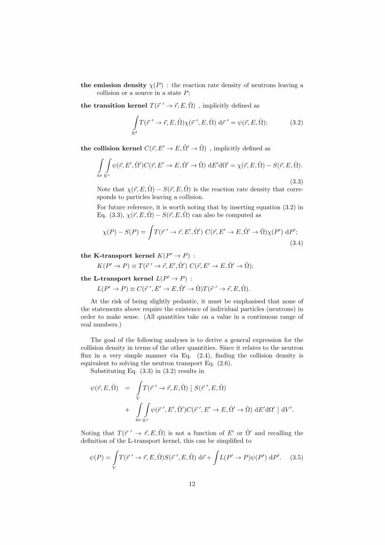
the emission density χ(P ) : the reaction rate density of neutrons leaving acollision or a source in a state P ;

the transition kernel T (~r ′ → ~r,E, Ω) , implicitly defined as∫R3

T (~r ′ → ~r,E, Ω)χ(~r ′, E, Ω) d~r ′ = ψ(~r,E, Ω); (3.2)

the collision kernel C(~r,E′ → E, Ω′ → Ω) , implicitly defined as∫4π

∫R+

ψ(~r,E′, Ω′)C(~r,E′ → E, Ω′ → Ω) dE′dΩ′ = χ(~r,E, Ω)− S(~r,E, Ω).

(3.3)Note that χ(~r,E, Ω) − S(~r,E, Ω) is the reaction rate density that corre-sponds to particles leaving a collision.

For future reference, it is worth noting that by inserting equation (3.2) inEq. (3.3), χ(~r,E, Ω)− S(~r,E, Ω) can also be computed as

χ(P )− S(P ) =

∫T (~r ′ → ~r,E′, Ω′) C(~r,E′ → E, Ω′ → Ω)χ(P ′) dP ′;

(3.4)

the K-transport kernel K(P ′ → P ) :

K(P ′ → P ) ≡ T (~r ′ → ~r,E′, Ω′) C(~r,E′ → E, Ω′ → Ω);

the L-transport kernel L(P ′ → P ) :

L(P ′ → P ) ≡ C(~r ′, E′ → E, Ω′ → Ω)T (~r ′ → ~r,E, Ω).

At the risk of being slightly pedantic, it must be emphasised that none ofthe statements above require the existence of individual particles (neutrons) inorder to make sense. (All quantities take on a value in a continuous range ofreal numbers.)

The goal of the following analyses is to derive a general expression for thecollision density in terms of the other quantities. Since it relates to the neutronflux in a very simple manner via Eq. (2.4), finding the collision density isequivalent to solving the neutron transport Eq. (2.6).

Substituting Eq. (3.3) in (3.2) results in

ψ(~r,E, Ω) =

∫V

T (~r ′ → ~r,E, Ω) [ S(~r ′, E, Ω)

+

∫4π

∫R+

ψ(~r ′, E′, Ω′)C(~r ′, E′ → E, Ω′ → Ω) dE′dΩ′ ] dV ′.

Noting that T (~r ′ → ~r,E, Ω) is not a function of E′ or Ω′ and recalling thedefinition of the L-transport kernel, this can be simplified to

ψ(P ) =

∫V

T (~r ′ → ~r,E, Ω)S(~r ′, E, Ω) d~r +

∫L(P ′ → P )ψ(P ′) dP ′. (3.5)

12

The collision density can be decomposed into several components that cor-respond to different amounts of collisions since emission from a source:

ψ(P ) =

∞∑i=0

ψi(P ), (3.6)

where ψl(P ) is the reaction rate density for collisions in which the neutronentering the collision has had l previous collisions. ([4], 11-12) The sum of the(direct) contributions of the sources to ψ(P ) is simply ψ0(P ):

ψ0(P ) =

∫V

T (~r ′ → ~r,E, Ω)S(~r ′, E, Ω) d~r ′. (3.7)

Of course, collisions corresponding to ψn+1(P ) are a result of collisions corre-sponding to ψn(P ). This implies that ψn+1(P ) depends on ψn(P ) via Eq. (3.5),where it should be noted that the source has no (direct) contribution to ψn(P )for n ≥ 1.

ψn+1(P ) =

∫(R,R+,〈4π〉)

ψn(P ′)L(P ′ → P ) dP ′ ∀ n ∈ N\0

By means of induction, a direct formula for ψk can now be found:

ψk(P ) =

∫. . .

∫ (ψ0(P0)

k−1∏x=0

L(Px → Px+1)

)k−1∏y=0

dPy.

Finally, recalling Eq. (3.6),

ψ(P ) = ψ0(P ) +

∞∑k=1

[∫. . .

∫ (ψ0(P0)

k−1∏x=0

L(Px → Px+1)

)k−1∏y=0

dPy

], (3.8)

where ψ0(P ) is given by Eq. (3.7).

In and of itself, this is quite an achievement. For example, if S does notdepend on ψ (i.e.: if there is no fission and only an external source), a directcomputation of the collision density is now possible using equations (3.7) and(3.8).

Note ψ, and thus the neutron flux, are only determined up to an integrationconstant. In the rest of this thesis, two fluxes are considered equivalent if theyare a multiple of each other.

The problem, of course, is that conventional numerical methods for integrat-ing over many dimensions are clumsy at best. Fortunately, it is in the evaluationof such integrals in hyperspace that the Monte Carlo method thrives. To im-plement a Monte Carlo analysis, a radically new interpretation of the transitionand collision kernels is necessary. (The reader is advised to review appendix Aat this point.)

First make a few observations:

13

1. There are no negative angular neutron fluxes or reaction rates. Therefore,T and C are always either positive or zero, and thus the same holds forthe K- and L-transport kernels.

2. Both the energies E and E′ and the directions Ω and Ω′ in C(~r,E →E′, Ω → Ω′) will always lie in Ω, E-space. Also, ~r, ~r′ ∈ R3 in T (~r →~r ′, E, Ω).

K and L can therefore both be viewed as functions that map a point inP -space to another point in P -space.

3. Eq. (3.2) is linear. Specifically, it is additive: if ψ1 and ψ2 are solutionsto χ1 and χ2 respectively, then ψ1 + ψ2 will be the solution to χ1 + χ2.Therefore, T is a function that maps a point from position space to anotherpoint in position space.

Similarly, from its definition (3.3), it follows that C is an additive kernelthat maps a point from E, Ω-space to another point in E, Ω-space.

Therefore, both K and L are additive as well.

Next, define a probability space with the whole of P -space as its sample space.It now becomes apparent that the statements above are equivalent to the Kol-mogorov axioms from appendix A.1 if T and C (and thus K and L) are regardedas (joint) probability density functions. A point in P -space satisfies Eq. (A.1)and is thus a stochastic variable. The process (P0, P1, . . .) is therefore a time-homogeneous Markov chain (appendix A.2).

This justifies the use of the Monte Carlo method to approximate ψ. Thatis, if the source distribution is known, the collision density can be found bysampling from the kernels in equations (3.7) and (3.8).

3.3 Source iteration

If the average number of new fission particles per collision reaction is knownand there are no external sources, then S can be found from ψ. The problemis that S is, in turn, needed to approximate ψ. To solve this issue, the Markovchain Monte Carlo method (a variation on the power method) is used. (Readersunfamiliar with this are referred to appendix A.2.)

First, sample from a homogeneous source distribution S(0).3 Now use thisdistribution to calculate a collision density ψ(1). Next, use ψ(1) to calculate anew source distribution S(1), which is used to determine a collision density ψ(2),and so on and so forth. Since S(n) depends solely on ψ(n), which depends solelyon S(n−1), the stochastic process (S(0), S(1), . . .) is a Markov chain.

If the system is critical and S(n) is the actual source, then S(n+1) = S(n).Therefore, the real source distribution is the stationary distribution of theMarkov process. From equations (A.2) and (A.3) it follows that it must alsobe the limiting distribution. The limiting distribution can be approximated byS(I) for some large I.

Obviously, this will not work well if the system isn’t critical, but there’s amethod of solving this, as will be explained in section 3.5.

3Actually any distribution should do, though it seems best not to start with a pointsource. [5]

14

The process of simulating the Markov chain and letting it converge to S iscalled source iteration or source convergence. Every step in the Markovchain is called a cycle. To avoid the enormous computational effort of havingto perform the source iteration many times, many source distributions in theset S(m),m ≥ I are used in a Monte Carlo calculation. These are referred toas the inactive cycles. The rest of the cycles are called active.

3.4 Particle histories

3.4.1 Sampling from the kernels

χ(P ) can be written as a weighted linear combination of hyper-dimensionalDirac delta functions δ(P ) in P -space. (χ(P ) ≡

∫χ(P ′)δ(P ′ − P ) dP ′) Recall

that the equation that defines the transition kernel T is linear. Therefore,in order to determine how to sample from the transition kernel, it suffices toconsider only the case that χ(~r,E, Ω) = δ(~r∗, E, Ω) for an arbitrary (~r∗, E, Ω).

The physical interpretation of this situation would be that there is a singleparticle that leaves a collision or source (i.e.: start a flight path) in the state(~r∗, E, Ω). ψ would then be the collision density resulting from a single neutronthat starts a flight path.

From Eq. (3.2), the collision density is

ψ(~r,E, Ω) = T (~r∗ → ~r,E, Ω) .

(The particle is ‘smeared out’ over P -space.)Since the transition kernel T (~r∗ → ~r,E, Ω) can be interpreted as a probabil-

ity density function, it can be sampled by assigning probabilities to the eventof a single neutron starting a trajectory at (~r∗, E, Ω) to have its next collisionin d~r,dE,dΩ at (~r,E, Ω).

In fact, by a similar reasoning, one can also simplify the interpretation ofthe other kernels in section 3.2 considerably:

• C(~r,E′ → E, Ω′ → Ω)] is the probability density for a particle entering acollision at ~r with energy E′ and direction Ω′ to have energy and directionE, Ω after the collision;

• K(P ′ → P ) is the probability density for a particle to go from P ′ to Pby first starting a trajectory from ~r ′ and then colliding at ~r to change itsenergy and direction;

• L(P ′ → P ) is the probability density for a particle to go from P ′ to Pby first changing energy and direction in a collision at ~r ′ and starting aflight path to the next collision at ~r.

Note that equations (3.7) and (3.8) are a direct result of equations (3.2)and (3.3). Thus, they are equivalent to the neutron transport equation (2.6),provided that the particle mentioned above has the same properties as a neu-tron. In other words, generating the Markov chain (P1, P0, . . .). comes down togenerating the ‘life’ of a neutron from the time it comes into being till the timeit is absorbed or leaks out of the system. Such a ‘life’ of a particle is called ahistory.

15

3.4.2 Simulating neutrons

A simulated neutron will start travelling from its initial position in a randomdirection. In this thesis, only neutrons that scatter isotropically are consid-ered. (I.e.: all directions in which the neutron can travel after a collision areequally probable.) In appendix B.3 it is explained how such a direction vectoris sampled.

After ‘choosing’ a direction, the neutron will start its trajectory, after whichit will either leak out of the system or enter a collision at some random distancefrom the initial position. From Eq. (2.3) and appendix B.2, it follows that thedistance to the next collision in a homogeneous medium can be sampled by

d = − 1

ΣTlog (ρ) , (3.9)

where ρ is uniformly distributed from 0 to 1.A neutron has no memory. In a medium with a piecewise constant total cross

section, the particle can thus be stopped when it enters a different segment. Anew random distance can then be sampled in the new segment.

In a medium with a continuously changing total cross section, a methodcalled hole tracking can be used. One simply adds a ‘dummy reaction’ witha continuously changing woodcock cross section ΣWC , such that the totalcross section is constant. If a particle enters a woodcock collision, it starts a newtrajectory with the same energy and direction. Unfortunately, this method israther inefficient if ΣT has a great spatial variance, since in that case ΣWC/ΣTcan be far larger than zero.

If a neutron enters a collision, several different types of nuclear reactionscan occur. In this thesis, only three will be considered: capture, scattering andfission reactions. The corresponding cross sections are respectively Σc, Σs andΣf , so ΣT = Σc + Σs + Σf . For simplicity, all neutrons will be considered tohave the same energy, so all scattering is elastic. The probability for a reactionof type 〈j〉 to occur, conditional on the event that a reaction occurs, is Σ〈j〉/ΣT .

In the event of absorption (fission or capture), the history ends. In casea scattering reaction is selected, a new direction is sampled and the neutronstarts a new path. If a fission reaction occurs, an integer number of new fissionneutrons is sampled. The source S(x) consists of all fission neutrons that weregenerated in cycle x.

In a typical calculation, the number of simulated histories is in the range103− 105, whilst the total number of cycles has an order of magnitude of 102−104.

3.5 Criticality calculation using the Monte Carlomethod

The criticality k can be estimated using the neutron histories. In principle, thiscan be done by counting the number of neutrons in a cycle and divide it by thenumber of neutrons in the previous cycle. The number of neutrons in cycle n

16

should be about k times as big as the number of neutrons in cycle n− 1. [1]

k = E[

fission neutrons generated in cycle j + 1

fission neutrons generated in cycle j

](3.10)

However, the number of simulated histories might grow exponentially or dieout if several cycles are generated. This will quickly turn into a serious problemwhen simulating the Markov chain (S(0), S(1), . . .), so a ‘trick’ has to be appliedto ensure that the number of simulated neutrons is more or less the same forevery cycle.

To this end, modify Eq. (3.4):

χ(P ) =1

k′S(P ) +

∫K(P ′ → P )χ(P ′) dP ′. (3.11)

This means that the number of neutrons that start a flight path at a sourceis reduced by a factor (k′)−1. (To achieve this, the average number of newneutrons in a fission reaction is multiplied by (k′)−1.) If k′ = k, the numberof neutrons that originate from fission sources is constant for every cycle. Eq.(3.11) is therefore an eigenvalue equation. Solving it comprises finding the valuefor k′ for which

∫χ(P ) dP is constant for all cycles.

Since this is not a deterministic calculation, the number of neutrons thatare generated in a cycle might still be different from the expected number offission neutrons. To compensate for this, the average number of fission neutronsgenerated per fission reaction in cycle j is multiplied by N?/Nj , where Nj is thenumber of neutrons at the start of the cycle and N? is the nominal number ofneutrons. On average, N? histories are generated per cycle.

Summarising, in cycle j the average number of new neutrons simulated in theevent of fission should be ν? = ν/k′(N?/Nj), where ν is the (actual, physical)average number of fission neutrons created in the event of fission. In the firstcycle, an initial guess of ν∗ = ν can be used.

Note that the estimator for k from formula (3.10) will no longer work. For-tunately, this is easily solved by multiplying the estimator with k′(Nj/N

?).For each cycle the value of k′ that is used in Eq. (3.11) is the estimate of

k that was calculated with Eq. (3.14) in the previous cycle. In theory, theexpectation value of k′ will converge to k after some amount of inactive cycles,so the criticality can be estimated as the average value of k′ over all the activecycles.

3.6 The scoring method

Several interesting quantities can be calculated by keeping track of how the(simulated) neutrons behave. Specifically, one can keep scores during the sim-ulation of the histories. To illustrate this concept, consider the problem of tryingto estimate the average flux in a volume.

From equations (2.5) and (2.4), the total reaction rate density (correspondingto any collision) is ΣTφ. But this is just equal to the collision density, which caneasily be determined using the neutron histories. Simply determine the average

17

number of times a neutron has a collision in the volume. To determine the flux,note that φ = ψ/ΣT . Now the flux can be approximated with the estimator

φ =1

N∗V

∑i

(1

ΣT

)ci

, (3.12)

where V is the size of the volume in which the flux is estimated and ci is theith collision. This means that each time a neutron enters a collision, a value of1/ΣT is counted.4

In general, such a value is called a tally, whilst the sum of all tallies isreferred to as the score. Tallying is the process of counting (scoring) thetallies. [1]

Sometimes there are several tallying methods to estimate the same quantity.For example, Sjenitzer ([4], 15-17) derives the following estimator for the averageflux on a surface:

φ =1

N∗A

∑j

(1

|µ|

)j

, (3.13)

where A is the area of the surface. The summation runs over all crossings j ofthe surface at an angle µ with the normal vector.

3.7 Standard variance reduction methods

If the variance of the samples in a Monte Carlo calculation is high, an accurateanswer can only be achieved by generating a large amount of samples. This canbe very costly and make the calculation impractical. Therefore, various variancereducing methods have been developed. They should reduce the time needed tomake an accurate guess of the final answer.

In this section some standard variance reducing methods will be discussed.All of these have been incorporated in every calculation in this thesis.

Instead of sampling the reaction type in the event of a collision, the differenttypes of reactions can be made implicit in every collision.

For example, instead of determining whether a fission event took place andsampling the number of fission neutrons from a predetermined distribution, newneutrons are created after each collision. The average number of new neutronsafter any collision should be equal to ν?Σf/ΣT , since that’s the expectationvalue for the number of fission neutrons, conditional on the event of a collision.

The final result of the Monte Carlo simulation will remain unbiased aslong as the average number of new fission neutrons created after a collisionis unchanged. Therefore, one can simply sample bν?Σf/ΣT c5 neutrons withprobability bν?Σf/ΣT c − ν? + 1 or bν?Σf/ΣT c + 1 neutrons with probabilityν? − bν?Σf/ΣT c.

Absorption can also be made implicit by gradually letting a neutron ‘die’a little after each collision. To facilitate this, a weight factor is introduced.A particle with weight w is considered to be wth of a particle. If it enters a

4In general, the cross sections may not be constant in space; it could be that ΣT is differentfor each collision.

5Here b−c is the floor operator.

18

collision, it will create w(ν?Σf/ΣT ) new neutrons on average after each collision.All tallies should also be multiplied by the weight.

The probability a neutron will end its history conditional on the event ofa collision is Σa/ΣT .6 Thus, instead of sampling the event of absorption, theweight of a neutron is reduced by a factor of 1− Σa/ΣT every time it leaves acollision. The weight of a neutron that has just been born is usually unity.

Implicit absorption and implicit fission reduce variance, because the neutronsbehave more alike. Instead of letting the histories stop abruptly at arbitrarypoints, weighting allows the particles to be ‘smeared out’. Instead of havinga few points with lots of fission neutrons, the new neutrons are more evenlydistributed.

Along the same line of reasoning, a better estimator for k can be derived.If Σf is the cross section for fission reactions, then ‘physical’ neutrons (not thesimulated ones) will create νΣf/ΣT fission neutrons on average in an arbitrarycollision. Thus a new estimator for the criticality would be

k =E [number of new fission neutrons generated in cycle j]

neutrons started in cycle j

=1

N∗

∑i

(νΣf/ΣT )ci . (3.14)

The summation runs over all collisions ci in cycle j. This is just another ex-ample of estimating a quantity with the scoring method. This time the tally isνΣf/ΣT . (Again, it might have a different value for every collision.)

A problem with implicit absorption is that it may take a very long time tosimulate histories, since they are only stopped once a particle leaks out of thesystem. Furthermore, a particle with a low weight will not contribute signifi-cantly to the final result of the calculation, so it is a waste to spend a lot ofcalculation time on it.

This can be solved in the following manner. Suppose the weight w? of theparticle drops below a predetermined limit wRR. It will then undergo Russianroulette. The particle has a probability of survival of wsur and a probability1 − wsur of getting killed (‘shot’), in which case the history is ended. If theparticle survives, the weight is set to a new value of w?/wsur. Russian rouletteis guaranteed not to introduce a bias, because the expectation value of the newweight of the particle is equal to the old weight:

P [survival] (weight after survival) + P [getting shot] (weight after getting shot)

= (wsur) (w?/wsur) + (1− wsur) 0 = w?.

A higher value of wRR increases the variance, but reduces the computationtime.

3.8 Difficulties

There are still some difficulties in implementing the Monte Carlo method forneutron transport. Some of them are listed here. They will be discussed in moredetail in later chapters.

6Remember that Σa is the absorption cross section, and that it includes both capture andfission.

19

1. Despite the efforts from the previous section, it may still take a largecomputational effort to make a reasonably accurate estimate of the desiredquantity. This is especially true for estimating quantities in regions wherethere is a low flux. Few simulated neutrons will travel there, so there willbe few tallies and thus a greater uncertainty is involved in estimating theaverage.

2. A more fundamental problem arises from the fact that the source iterationis performed only once and several sources in the source iteration are used.Since the S(m),m ≥ M will, in general, be correlated, it is difficult todetermine the standard deviation of the estimations of the criticality inthe cycles. This makes it impossible to determine the error in the finalanswer.

3. It is not easy to verify that the source distribution converges at the sametime the estimations of k do. Also, the power method does not guaranteethat the source distribution will converge to the flux at all if there arelocal minima.

Consider a situation where there are two or more regions where fissionmight occur that are separated by several mean free paths of the neutronand all neutron start in just one of the regions. Physically, if some of theneutrons cross over to another region, they might multiply there. However,if the total number of simulated histories per cycle is kept approximatelyconstant at N∗. Therefore, it may well be that the neutrons that crossedover die out after some cycles, since their total number is kept low.

Systems like these are called loosely coupled. Their most well-knownoccurrence is in the storage of used-up fuel assemblies, where there isusually some material in between the fuel assemblies.

20

Chapter 4

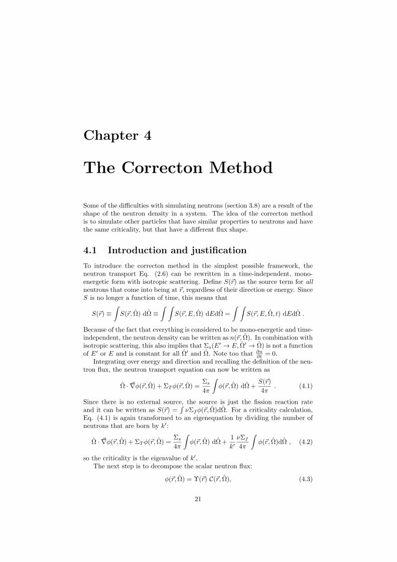
The Correcton Method

Some of the difficulties with simulating neutrons (section 3.8) are a result of theshape of the neutron density in a system. The idea of the correcton methodis to simulate other particles that have similar properties to neutrons and havethe same criticality, but that have a different flux shape.

4.1 Introduction and justification

To introduce the correcton method in the simplest possible framework, theneutron transport Eq. (2.6) can be rewritten in a time-independent, mono-energetic form with isotropic scattering. Define S(~r) as the source term for allneutrons that come into being at ~r, regardless of their direction or energy. SinceS is no longer a function of time, this means that

S(~r) ≡∫S(~r, Ω) dΩ ≡

∫ ∫S(~r,E, Ω) dEdΩ =

∫ ∫S(~r,E, Ω, t) dEdΩ .

Because of the fact that everything is considered to be mono-energetic and time-independent, the neutron density can be written as n(~r, Ω). In combination withisotropic scattering, this also implies that Σs(E

′ → E, Ω′ → Ω) is not a functionof E′ or E and is constant for all Ω′ and Ω. Note too that ∂n

∂t = 0.Integrating over energy and direction and recalling the definition of the neu-

tron flux, the neutron transport equation can now be written as

Ω · ~∇φ(~r, Ω) + ΣTφ(~r, Ω) =Σs4π

∫φ(~r, Ω) dΩ +

S(~r)

4π. (4.1)

Since there is no external source, the source is just the fission reaction rateand it can be written as S(~r) =

∫νΣfφ(~r, Ω)dΩ. For a criticality calculation,

Eq. (4.1) is again transformed to an eigenequation by dividing the number ofneutrons that are born by k′:

Ω · ~∇φ(~r, Ω) + ΣTφ(~r, Ω) =Σs4π

∫φ(~r, Ω) dΩ +

1

k′νΣf4π

∫φ(~r, Ω)dΩ , (4.2)

so the criticality is the eigenvalue of k′.The next step is to decompose the scalar neutron flux:

φ(~r, Ω) = Υ(~r) C(~r, Ω), (4.3)

21

where Υ is a function of position only. C(~r, Ω) can be considered a multiplicativecorrection of Υ. After some manipulation (ref. [4], 25-26,41), substituting Eq.(4.3) in Eq. (4.2) results in

Ω · ~∇C(~r, Ω) +[ΣT + Ω · ~∇ ln Υ(~r)

]C(~r, Ω)

=Σs4π

∫C(~r, Ω) dΩ +

1

k′νΣf4π

∫C(~r, Ω) dΩ . (4.4)

Comparing this to the neutron transport equation (4.2), it is apparent thatthe only difference is that φ is replaced by C and some value has been addedto the total cross section. Note however, that it is still an eigenequation, sothe criticality can still be calculated by solving the equation by means of theMarkov chain Monte Carlo (MCMC) power method.

Since φ can be estimated by simulating particles histories in a Monte Carlocalculation, the same can be done for C. (Although it may seem very abstractphysically to simulate self-made particles, mathematically it isn’t any strangerthen simulating the neutron transport equation with neutrons.)

These new particles are called correctons. The only difference with neu-trons they have an effective total cross section of

ΣcT = ΣT + Ω · ~∇ ln Υ(~r) . (4.5)

Because their fission and scattering cross sections are the same as for neutrons,their absorption cross section should be

Σca = Σa + Ω · ~∇ ln Υ(~r) .1 (4.6)

Simulating correctons only requires a minor manipulation of the simulationof neutrons. The only difference is that some of the cross sections depend onthe position and direction of the neutron. Therefore, the tallies and the num-ber of new correctons in the event of implicit fission differ from those of neutrons.

From the previous discussion, it is still unclear why the correcton methodwould provide better results than a regular simulation with neutrons. The mainadvantage is that correctons can be steared by the choice of Υ.

For a particle that moves towards a greater value of φ(~r), Ω · ~∇ ln φ(~r) ispositive. This means that the total cross section is greater, so the correctondoesn’t travel very far. Conversely, if the particle is moving towards a positionwhere φ(~r) is smaller, Ω · ~∇ ln φ(~r) will have a negative value and the correctonwill travel a bit further than a neutron would have done.

Sjenitzer [4] used this to do a more efficient calculation of the flux at alarge distance from a source, by choosing Υ in such a way that the correctonswere directed towards the region of interest. Huisman [8] extended this to threedimensions.

1To avoid confusion, Σa and ΣT are still used to denote the cross sections for neutrons.Correcton cross sections will be indicated by the superscript c.

22

4.2 The choice of Υ(~r)

4.2.1 Limitations

Equations (4.5) and (4.6) seem to put some restrictions on the choice of Υ(~r).A negative total cross section not only has no physical interpretation, but (moreimportantly) it also renders sampling a random distance with Eq. (3.9) impos-sible. Therefore, Υ must be chosen in such a way that

min(

ΣT + Ω · ~∇ ln Υ(~r))> 0 .

Recalling that∣∣∣Ω∣∣∣ ≡ 1, it is obvious that arg min

Ω

(Ω · ~∇ ln Υ(~r)

)= − ~∇ ln Υ(~r)

|~∇ ln Υ(~r)|and thus the equation above simplifies to∣∣∣~∇ ln Υ(~r)

∣∣∣ < ΣT ∀ ~r . (4.7)

Note that this does not guarantee that Σca > Σf or even Σc

a > 0. However, itis not so clear whether this is problematic when the method of implicit absorp-tion from section (3.7) is used. A negative absorption cross section leads to anincrease in the weight of the particle if it enters a collision. This should not posea problem, since the effects of absorption are only implicitly present in the sec-ond term on the rhs of Eq. (4.4). The production term (vΣf/4π)

∫C(~r, Ω) dΩ

also remains unaffected if the absorption cross section drops below the fissioncross section.

Without mentioning it explicitly, Becker [6], Becker et al. [5] and Huisman[8] have all used negative absorption cross sections without encountering anydifficulties.

Since the neutron flux is continuous, Eq. (4.3) implies that discontinuitiesin Υ(~r) should be compensated by discontinuities in C(~r, Ω). These do notnaturally occur in the flux profile of correctons. Therefore, discontinuities willhave to be ‘artificially’ implemented in C. This can easily be done by changingthe weight of particles that cross some discontinuity in Υ.

Specifically, if a particle is in the state (~r, Ω), then

limε↓0

φ(~r − εΩ, Ω

)= lim

ε↓0φ(~r + εΩ, Ω

)implies

limε↓0

C(~r + εΩ, Ω

)C(~r − εΩ, Ω

) = limε↓0

Υ(~r − εΩ, Ω

)Υ(~r + εΩ, Ω

) (4.8)

and thus the weight of a correcton has to be multiplied by limε↓0Υ(~r−εΩ,Ω)Υ(~r+εΩ,Ω)

when crossing a discontinuity in Υ.Note that this is invalid if Υ = 0, but equation (4.3) rules out this choice

anyway.

23

4.2.2 Mathematical representation

In this thesis, the systems under consideration are rectangular parallelepipedsthat are subdivided by smaller cells that are also rectangular parallelepipeds.The material properties are homogeneous within the cells. Υ(~r) is chosen to bepiecewise continuous, that is, it is continuous within the cells.

Let x, y and z be cartesian coordinates, so that ~r = [x, y, z]T

. The index ofa cell is denoted by (i, j, k), meaning that it is the ith cell in the x-direction, the

jth cell in the y-direction and the kth cell in the z-direction. Let ~Oi,j,k be thecentre of the cell.

To avoid the necessity of using hole tracking, the cross sections have tobe constant for particles travelling through a cell. If Υi,j,k (~r) is the functiondescribing Υ (~r) in cell (i, j, k), it must be of the form

~∇ ln Υi,j,k(~r) = constant

⇒ ln Υi,j,k(~r) = ~βi,j,k · ~r +(

ln(Ki,j,k)− ~βi,j,k · ~Oi,j,k)

⇒ Υi,j,k(~r) = Ki,j,k exp[~βi,j,k ·

(~r − ~Oi,j,k

)], (4.9)

for some parameters ~βi,j,k and Ki,j,k.Eq. (4.7) now takes on the particularly simple form∣∣∣~βi,j,k∣∣∣ < (ΣT )i,j,k , (4.10)

where (ΣT )i,j,k is the total cross section in cell (i, j, k). Eq. (4.9) with |~βi,j,k| →(ΣT )i,j,k is also the function that maximises the slope of Υ(~r) constraint by(4.7). For some given total cross section ΣT in a material without fission, theneutron flux has a maximum slope if ΣT = Σa, in which case the flux willdecrease exponentially and it can only just be described by Eq. (4.9).

4.3 Real time flux estimation

Suppose that Υ(~r) is a reasonably good estimate φ(~r) of the scalar neutron fluxφ(~r) ≡

∫φ(~r,Ω) dΩ, meaning that it has more or less the same shape:

φ (~r) ∝ φ (~r) .

According to Eq. (4.3), the correcton flux C should be roughly constant. Thismay enhance the convergence of the correcton flux distribution, since the cor-rectons do not have a tendency to pile up in some region.

The flux guess may be obtained from a cheap Monte Carlo calculation ora deterministic calculation. To enhance the source convergence, it might evensuffice if the flux distribution is only qualitatively correct.

In this thesis, a real time flux estimation is proposed. The idea is to tallythe flux of the correctons during every cycle and use the results to make betterand better estimations of the neutron flux. These new estimations can then beused to adjust Υ(~r) to make it a better representation of the neutron flux.

The two main difficulties are

24

• determining a φ (~r) from a simulation with correctons;

• adjusting the flux parameters Ki,j,k and ~βi,j,k to make Υ(~r) as close aspossible to the actual flux shape.

These are dealt with in sections 4.4 and 4.5 respectively.

Note that Υ is, in general, different for every cycle. Therefore, the particleshave to converge to a different flux distribution in every cycle. To solve thisproblem, the weights of the particles at the beginning of their history can beadjusted in order change the flux distribution they represent.

Specifically, if Υi is used to perform the calculations in cycle i and Ci = φ/Υi,then the correcton flux in cycle j is a multiple of what it was in cycle j − 1:

Cj(~r,Ω)

Cj−1(~r,Ω)=

φ(~r,Ω)/Υj(~r)

φ(~r,Ω)/Υj−1(~r)=

Υj−1(~r)

Υj(~r)(4.11)

Thus, the weight of a particle at ~r at the beginning of its history in cycle j must

be set toΥj−1(~r)Υj(~r)

.

4.4 Estimating the neutron flux from correctonhistories

The correcton flux can be obtained by tracking the positions of the correctons.The neutron flux equals Υ multiplied by the correcton flux. Therefore, theneutron flux can be found by counting every correcton at ~r as Υ(~r) particles.

Therefore, one can simply tally the neutron flux by using Eq. (3.12) or Eq.(3.13) and multiplying every tally at ~r with Υ(~r).

In this thesis, in every calculation the neutron surface flux was estimated.Compared to using average fluxes, this makes it easier to adjust the parametersof Υ(~r) to the neutron flux shape if Υ(~r) is given by Eq. (4.9).

Suppose a correcton travelling in a direction Ω has a weight w before itcrosses from one cell to another at ~r. Before it crossed the cell boundary, it wascounted as w limε↓0 Υ(~r − εΩ) neutrons. Since the correcton changes it weight,

it is still counted as(w

limε↓0 Υ(~r−εΩ)

limε↓0 Υ(~r+εΩ)

)limε↓0 Υ(~r + εΩ) = w limε↓0 Υ(~r − εΩ)

neutrons after crossing the cell. (This is hardly surprising, since the neutronflux is a continuous quantity.)

It seems best not to change the Υi,j,k in every cycle, but instead to let thetallies accumulate over several cycles and only then to determine a new fluxestimate. There are two principle reasons for this. First, it is possible that notall boundaries have been crossed by a particle after just one cycle. This meansthat the estimate of the average correcton flux over some of the boundariesmight be zero, in which case none of the analyses in section 4.5 makes sense.

Secondly, there will be less statistical variation in the surface flux estimates.Therefore, one would expect to see fewer cases where adjacent cells have a largediscontinuity in Υ (~r).

To ensure that the tallies in every cycle have approximately the same amountof influence on the final estimate of the neutron flux, the sum of the flux esti-mates over all boundaries should be normalised in every cycle.

25

4.5 Estimating the flux parameters

Every cell has six boundaries, whilst there are only four degrees of freedom inthe parameters ~βi,j,k and Ki,j,k. In general, it is therefore impossible to satisfyall boundary conditions. However, the correcton flux can still be made flatter,and thus more stable, if only Υ has more or less the same shape as the neutronflux.

Since ~∇ ln Υi,j,k(~r) depends solely on the ~βi,j,k, the Ki,j,k do not influencethe cross sections of the particles. However, the weight change of the particle iseffected by the choice of the Ki,j,k via Eq. (4.8).

If the weight multiplication is very large, some particles will have very highweights. Big differences between the weights of the particles lead not only to ahigher variance in the calculation, but can also result in large concentrations ofnew fission particles, which can destabilise the calculation.

Therefore, the task at hand is to choose the ~βi,j,k such that the correctonsare driven towards regions with a low neutron flux, whilst the Ki,j,k should beadjusted to make the weight changes of the particles crossing cells borders areas small as possible. Unfortunately, this is far from trivial.

4.5.1 Choosing ~βi,j,k

Suppose the lengths of the ribs of cell (i, j, k) in the x-, y- and z-direction are2Ai,j,k, 2Bi,j,k and 2Ci,j,k respectively. The estimated average neutron fluxes atthe boundaries of the cell are presumed to be known and equal Fi±,j,k, Fi,j±,kand Fi,j,k± for the boundaries ~r · x = ~Oi,j,k · x±Ai,j,k , ~r · y = ~Oi,j,k · y±Bi,j,kand ~r · z = ~Oi,j,k · z ± Ci,j,k respectively.2

One might choose the ~βi,j,k such that the multiplicative error between Υand and the neutron flux is equal for opposing boundaries, i.e.:

Υ( ~Oi,j,k · x+Ai,j,k, y, z)

Fi+,j,k=

Υ( ~Oi,j,k · x−Ai,j,k, y, z)Fi−,j,k

Υ(x, ~Oi,j,k · y +Bi,j,k, z)

Fi,j+,k=

Υ(x, ~Oi,j,k · y −Bi,j,k, z)Fi,j−,k

Υ(x, y, ~Oi,j,k · z + Ci,j,k)

Fi,j,k+=

Υ(x, y, ~Oi,j,k · z − Ci,j,k)

Fi,j,k−.

This leads to

~βi,j,k =

[1

2Ai,j,kln

(Fi+,j,kFi−,j,k

),

1

2Bi,j,kln

(Fi,j+,kFi,j−,k

),

1

2Ci,j,kln

(Fi,j,k+Fi,j,k−

)]T,

(4.12)regardless of Ki,j,k. However, this does not guarantee that the restriction (4.10)is met, so an adjustment is necessary. In an effort to maintain the shape of Υas much as possible, one may choose to multiply the ~βi,j,k with a factor that

2This isn’t a particularly elegant notation, since the same neutron flux can sometimes bedenoted in two different manners. (For example F2−,j,k ≡ F1+,j,k.) However, it is easy touse.

26

makes them satisfy Eq. (4.10):

~βi,j,k = min

((ΣT )i,j,k`i,j,k

, 1

) ln

(Fi+,j,kFi−,j,k

)2Ai,j,k

,

ln

(Fi,j+,kFi,j−,k

)2Bi,j,k

,

ln

(Fi,j,k+Fi,j,k−

)2Ci,j,k

T

,

(4.13)where, for convenience, the definition

`i,j,k ≡

√√√√√√√ ln

(Fi+,j,kFi−,j,k

)2Ai,j,k

2

+

ln

(Fi,j+,kFi,j−,k

)2Bi,j,k

2

+

ln

(Fi,j,k+Fi,j,k−

)2Ci,j,k

2

has been used.Note that the Fi±,j±,k± are usually different from one another, so none of the

cartesian components of ~βi,j,k are zero. So long as ~βi,j,k 6= ~0, the following anal-yses in this chapter is not fundamentaly changed, although some mathematicalresults are slightly different.

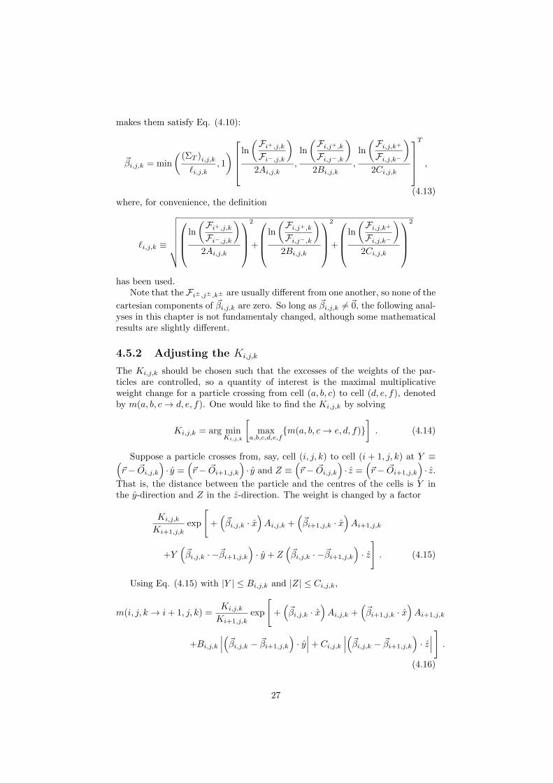
4.5.2 Adjusting the Ki,j,k

The Ki,j,k should be chosen such that the excesses of the weights of the par-ticles are controlled, so a quantity of interest is the maximal multiplicativeweight change for a particle crossing from cell (a, b, c) to cell (d, e, f), denotedby m(a, b, c→ d, e, f). One would like to find the Ki,j,k by solving

Ki,j,k = arg minKi,j,k

[max

a,b,c,d,e,fm(a, b, c→ e, d, f)

]. (4.14)

Suppose a particle crosses from, say, cell (i, j, k) to cell (i + 1, j, k) at Y ≡(~r − ~Oi,j,k

)· y =

(~r − ~Oi+1,j,k

)· y and Z ≡

(~r − ~Oi,j,k

)· z =

(~r − ~Oi+1,j,k

)· z.

That is, the distance between the particle and the centres of the cells is Y inthe y-direction and Z in the z-direction. The weight is changed by a factor

Ki,j,k

Ki+1,j,kexp

[+(~βi,j,k · x

)Ai,j,k +

(~βi+1,j,k · x

)Ai+1,j,k

+Y(~βi,j,k · −~βi+1,j,k

)· y + Z

(~βi,j,k · −~βi+1,j,k

)· z

]. (4.15)

Using Eq. (4.15) with |Y | ≤ Bi,j,k and |Z| ≤ Ci,j,k,

m(i, j, k → i+ 1, j, k) =Ki,j,k

Ki+1,j,kexp

[+(~βi,j,k · x

)Ai,j,k +

(~βi+1,j,k · x

)Ai+1,j,k

+Bi,j,k

∣∣∣(~βi,j,k − ~βi+1,j,k

)· y∣∣∣+ Ci,j,k

∣∣∣(~βi,j,k − ~βi+1,j,k

)· z∣∣∣ ] .

(4.16)

27

Similarly, the maximal multiplicative weight change of a particle crossing thesame border in the other direction is

m(i+ 1, j, k → i, j, k) =Ki+1,j,k

Ki,j,kexp

[−(~βi,j,k · x

)Ai,j,k −

(~βi+1,j,k · x

)Ai+1,j,k

+Bi,j,k

∣∣∣(~βi+1,j,k − ~βi,j,k

)· y∣∣∣+ Ci,j,k

∣∣∣(~βi+1,j,k − ~βi,j,k

)· z∣∣∣ ] .

(4.17)

Therefore, minimising the maximum relative weight change of particles crossingthe boundary between cell (i, j, k) and cell (i+1, j, k) in any direction comprisesminimising

max

Ki+1,j,k/Ki,j,k

exp[(Ai,j,k~βi,j,k +Ai+1,j,k

~βi+1,j,k

)· x] , exp

[(Ai,j,k~βi,j,k +Ai+1,j,k

~βi+1,j,k

)· x]

Ki+1,j,k/Ki,j,k

,

which leads to

Ki+1,j,k

Ki,j,k= exp

[(Ai,j,k~βi,j,k +Ai+1,j,k

~βi+1,j,k

)· x]

. (4.18)

Thus, if all ~βi,j,k are (anti)parallel to x, then the solution to Eq. (4.14)should satisfy Eq. (4.18). (The results are similar for particles crossing fromone cell to another in the y- or z-direction.)

Unfortunately, finding a closed-form solution to Eq. (4.14) is very difficultfor the general case. (In fact, it may well be impossible.)

Applying some physical insight, it seems reasonable that the estimate of theaverage neutron flux at the boundaries of a cell should be equal to the averagevalue of Υ at the boundaries. Ki,j,k can then be adjusted to ensure that∫∫

all 6 surfaces

Υ(x, y, z) dY =(Fi+,j,k + Fi,j+,k + Fi,j,k+ + Fi−,j,k + Fi,j−,k + Fi,j,k−

)(4.19)

The ‘x-boundaries’ of cell (i, j, k) (i.e.: the boundaries with normal vectors

that are (anti)parallel to x) are given by(~r − ~Oi,j,k

)· x = ±Ai,j,k and thus the

integrals of Υ over those surfaces are

~Oi,j,k·z+Ci,j,k∫z=~Oi,j,k·z−Ci,j,k

~Oi,j,k·y+Bi,j,k∫y=~Oi,j,k·y−Bi,j,k

dy dz Υi,j,k( ~Oi,j,k · x±Ai,j,k , y, z)

=Ki,j,k

(eBi,j,k(

~βi,j,k·y) − e−Bi,j,k(~βi,j,k·y)

)(eCi,j,k(

~βi,j,k·z) − e−Ci,j,k(~βi,j,k·z)

)e∓Ai,j,k(

~βi,j,k·x)(~βi,j,k · y

)(~βi,j,k · z

) ,(4.20)

with similar expressions for the other boundaries of the cell. The integral of

28

Υ(~r) over the total surface Y of the cell is thus∫∫all 6 surfaces

Υ(x, y, z) dY

= κ Ki,j,k

·

[(~βi,j,k · x

) eAi,j,k(~βi,j,k·x) + e−Ai,j,k(

~βi,j,k·x)

eAi,j,k(~βi,j,k·x) − e−Ai,j,k(

~βi,j,k·x)(4.21)

+(~βi,j,k · y

) eBi,j,k(~βi,j,k·y) + e−Bi,j,k(

~βi,j,k·y)

eBi,j,k(~βi,j,k·y) − e−Bi,j,k(

~βi,j,k·y)

+(~βi,j,k · z

) eCi,j,k(~βi,j,k·z) + e−Ci,j,k(

~βi,j,k·z)

eCi,j,k(~βi,j,k·z) − e−Ci,j,k(

~βi,j,k·z)

],

where

κ ≡(

eAi,j,k(~βi,j,k·x) − e−Ai,j,k(

~βi,j,k·x))

·(

eBi,j,k(~βi,j,k·y) − e−Bi,j,k(

~βi,j,k·y))(

eCi,j,k(~βi,j,k·z) − e−Ci,j,k(

~βi,j,k·z))

·(~βi,j,k · x

)−1 (~βi,j,k · y

)−1 (~βi,j,k · z

)−1

. (4.22)

For some given ~βi,j,k, Eq. (4.19) is solved for Ki,j,k by setting the rhs of 4.19equal to the rhs of 4.21.

29

Chapter 5

Numerical Examples

In this chapter, several statements that have been made throughout the previoustwo chapters are put to the test. Criticality calculations have been performedfor different systems. The neutrons are considered to be mono-energetic andthere are no delayed neutrons. This makes the systems wildly unrealistic froma physical point of view, but they serve to illustrate some of the points made inthe text.

First the theory from the previous chapters is put to the test for a simplehomogeneous rectangular parallelepiped, called system 1. Several simulationsshould convince the reader of the robustness of the proposed correcton method.

Then, a more complicated system of loosely coupled fuel assemblies, calledsystem 2, is studied. It is shown how a conventional neutron calculation fails,while the correcton method provides significantly better results.

Complete specifications of both systems can be found in appendix C.

In every calculation, all variance reducing techniques developed in section3.7 have been used (including implicit fission and absorption, Russian rouletteand the criticality tally (3.14)). The parameters for Russian roulette are alwayswRR = 0.1 and wsur = 0.5.

The total number of cycles is always denoted byM; the nominal number ofhistories per cycle is N∗.

5.1 System 1: a homogeneous rectangular par-allelepiped

5.1.1 Basic criticality calculation with neutrons

A basic criticality calculation with neutrons has been performed for system 1.The number of cycles was M = 105 and the average number of simulatedhistories per cycle was N∗ = 106.

Fig. 5.1 shows a typical realisation of the simulation. From the plot, it canbe seen how the criticality estimates converge to some value that is close to1. In the first cycles the neutrons are still more or less uniformly distributed.After the source converges, the particles are more concentrated in the centre

30

0 5 10 15 20 25 30 35 400.91

0.92

0.93

0.94

0.95

0.96

0.97

0.98

0.99

1

cycle

criti

calit

y es

timat

e

Figure 5.1: criticality estimates during first cycles of neutron calculation for ahomogeneous rectangular parallelepiped (system 1)

of the rectangular parallelepiped, so less particles will leak out of the system.Therefore, the criticality estimates are lower in the inactive cycles.

Suppose the first I = 100 cycles are taken to be the inactive cycles and thevalues of the criticality are considered to be i.i.d. This results in a criticalityestimate of k = 1.00013526 with a standard deviation of 7.7 · 10−7.

5.1.1.1 Estimating the error of the final result

Fig. 5.2 shows the values of the criticality estimates during some of the activecycles. Even with a Savitzky-Golay filter1 of order 10000, the estimates forthe criticality as a function of the cycle show a clear trending behaviour. Inother words, they are far from i.i.d. The positions of the particles in a cycle arestrongly positively correlated with the positions of the particles in the previouscycles. Therefore, the estimates of k are positively correlated as well. Thisrenders it very difficult to estimate the error of such a calculation.

The same calculation with M = 103 and N∗ = 106 has been performed 33times with 100 inactive cycles each time. This way, different final values of thecriticality were found. From this, it was determined that the standard deviationof the final answer of a single calculation is 1.4 ·10−5. If, however, the criticalityestimates in the active cycles of a single calculation are considered to be i.i.d.,the standard deviation in the final answer is estimated to be (8.1± 0.2) · 10−6,

1A Savitzky-Golay filter of order j is a generalised moving average filter, where the weightcoefficients are determined by a polynomial regression of order j. It should smooth a setof data, but compared to a moving average filter it preserves trending behaviour and localextrema better. (Orfanidis, S.J., Introduction to Signal Processing, Prentice-Hall, 1996)

31

1 2 3 4 5 6 7 8 91.25

1.3

1.35

1.4

1.45

cycle (⋅ 104)

(k−

1) ⋅

104

Figure 5.2: criticality estimates k during active cycles of neutron calculation fora homogeneous rectangular parallelepiped (system 1) (smoothed with Savitzky-Golay filter of order 104)

which is 1.7 times lower.In the following sections, the reported error is always based on the standard

deviation of the estimates of the criticality. The previous discussion suggeststhat it should be of the same order of magnitude as the actual error. However,due to positive correlation between the cycles, the true error is most likely larger.

5.1.2 Robustness tests for the correcton method

In this section, several extreme examples are used to test the robustness of thecorrecton method.

In every case, the neutron flux tallies have been compared to the flux talliesthat were obtained from a calculation with neutrons. The results were all indis-tinguishable. (The neutron flux in the x-, y- or z-direction have a typical cosineshape. This is a well-known result from analytical deterministic methods. ([2],209))

5.1.2.1 Criticality calculation with correctons for system 1

To facilitate a calculation with correctons, system 1 has been subdivided in twocells: (1, 1, 1) and (2, 1, 1). They are separated by the plane x = 5 cm.

Two different simulations have been done with M = 18500 and N∗ = 106

each. In the first case, ~β1,1,1 = (ΣT ) x and ~β2,1,1 = ~0. In the second calculation,~β1,1,1 = − (ΣT ) x and ~β2,1,1 = ~0. In both cases, the Ki,j,k have been calculatedwith Eq. (4.18). In this particular case, the Ki,j,k can be chosen in such a waythat there is no discontinuity in Υ(~r).

Plots of the criticality estimates can be found in figures 5.3 and 5.4. Inboth cases, the criticality converges to the same value as in section 5.1.1. The

32

20 40 60 80 100 120 140

1

1.02

1.04

1.06

1.08

1.1

1.12

1.14

1.16

1.18

cycle

criti

calit

y

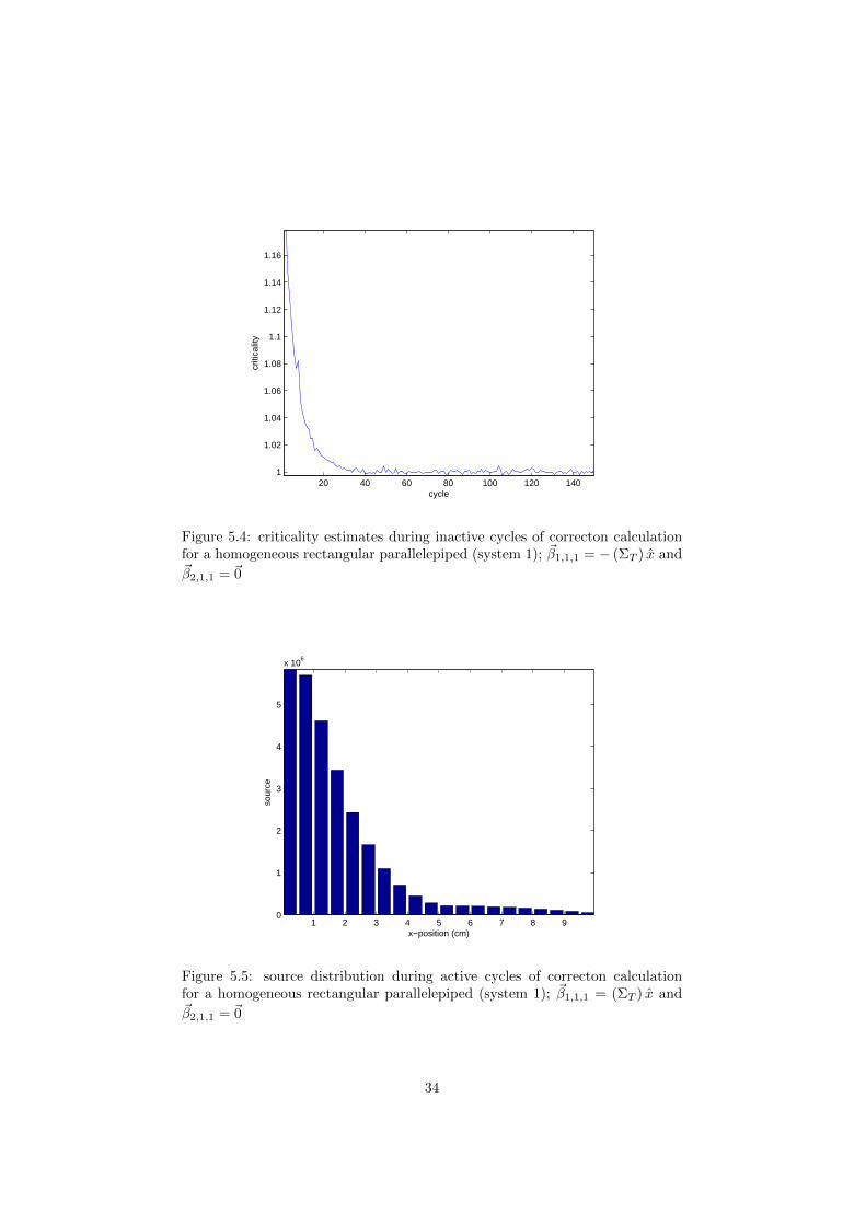
Figure 5.3: criticality estimates during inactive cycles of correcton calculationfor a homogeneous rectangular parallelepiped (system 1); ~β1,1,1 = (ΣT ) x and~β2,1,1 = ~0

number of inactive cycles is taken to be 50 in each. The estimates are k =1.000154± 3.4 · 10−5 and k = 1.000121± 1.3 · 10−5 respectively.

Figures 5.5 and 5.6 show the source distribution of the correctons for ~β1,1,1 =

(ΣT ) x and ~β1,1,1 = − (ΣT ) x respectively. These plots have been obtained byrandomly selecting 1500 particles after each cycle and storing their positionsat the beginning of their history. The y-axis indicates the number of timesa particle was found in a certain region during any of the active cycles. (Notethat only the relative frequencies with which the particles are in certain positionsbear any real meaning.)

Since the fission cross section is constant in the medium, and since there isno external source, the source distribution is proportional to the correcton fluxC. According to Eq. (4.3), C should be small in regions where Υ(~r) is very largeand vice versa. This is reflected in figures 5.5 and 5.6.

This calculation also confirms that there is no problem with negative ab-sorption cross sections for correctons.

5.1.2.2 Correctons with a discontinuous Υ(~r) in system 1

In the previous calculations, the values for ~βi,j,k and Ki,j,k were chosen in sucha way that that was no discontinuity in Υ(~r). To test the validity of changingthe particle weights via Eq. (4.8), a calculation with a discontinuous Υ(~r) hasalso been performed.

The medium in system 1 is subdivided in 24 cells (1, 1, 1), . . . , (1, 1, 24) thatare separated by the planes z = 1 cm, 2 cm, . . . , z = 23 cm. The parameters are~β1,1,k = ~0 ∀ k = 1, . . . , 24 (so Υ1,1,k(~r) = K1,1,k), whilst the K1,1,k have beenrandomly chosen from a uniform distribution from 1 to 11. M = 1.8 · 104 and

33

20 40 60 80 100 120 1401

1.02

1.04

1.06

1.08

1.1

1.12

1.14

1.16

cycle

criti

calit

y

Figure 5.4: criticality estimates during inactive cycles of correcton calculationfor a homogeneous rectangular parallelepiped (system 1); ~β1,1,1 = − (ΣT ) x and~β2,1,1 = ~0

1 2 3 4 5 6 7 8 90

1

2

3

4

5

x 106

x−position (cm)

sour

ce

Figure 5.5: source distribution during active cycles of correcton calculationfor a homogeneous rectangular parallelepiped (system 1); ~β1,1,1 = (ΣT ) x and~β2,1,1 = ~0

34

1 2 3 4 5 6 7 8 90

0.5

1

1.5

2

2.5

3

x 106

x−position (cm)

sour

ce

Figure 5.6: source distribution during active cycles of correcton calculation fora homogeneous rectangular parallelepiped (system 1); ~β1,1,1 = − (ΣT ) x and~β2,1,1 = ~0

N∗ = 106.The source distribution has been obtained in the same manner as in figures

5.5 and 5.6. The result is shown in Fig. 5.7.The initial criticality estimates are displayed in Fig. 5.8. If there are 100

inactive cycles, the criticality is estimated to be k = 1.0001325±3.5 ·10−6. Thismatches the estimates from the previous calculations, confirming the theoreticalfoundation of using a discontinuous Υ(~r).

5.1.2.3 Correctons with a changing Υ(~r) in system 1

In a real time flux estimation, Υ(~r) may have to be adjusted during a cal-culation. To test the method of adjusting the initial weight of the particlesat the beginning of their history (section 4.3; Eq. (4.11)), a calculation hasbeen performed where the value of Υ(~r) flips between Υ(1)(~r) in the odd cycles

and Υ(2)(~r) in the even cycles. They are characterised by (~β(1)i,j,k,K

(1)i,j,k) and

(~β(2)i,j,k,K

(2)i,j,k) respectively. At the beginning of each cycle, the total weight of

the particles is normalised to N∗.The system has been divided in the same cells as in the previous section.

The parameters are

~β(1)1,1,k =

12 (ΣT ) z , k = 1, . . . , 80 , k = 9, . . . , 16− 1

2 (ΣT ) z , k = 17, . . . , 24(5.1)

and~β

(2)1,1,k = −~β(1)

1,1,k (5.2)

35

2 4 6 8 10 12 14 16 18 20 220

0.5

1

1.5

2

x 106

z−position (cm)

sour

ce (

a.u.

)

Figure 5.7: source distribution during active cycles of correcton calculation for ahomogeneous rectangular parallelepiped (system 1) with a discontinuous, piece-wise constant Υ(~r)

5 10 15 20 25 30 35 40 45 50 55 60

0.98

0.985

0.99

0.995

1

1.005

1.01

1.015

1.02

cycle

criti

calit

y

Figure 5.8: criticality estimates during inactive cycles of correcton calculationwith a discontinuous, piece-wise constant Υ(~r)

36

5 10 15 20 25 30 35 40 45 50

0.96

0.97

0.98

0.99

1

1.01

1.02

1.03

cycle

criti

calit

y

criticality estimates

odd cycles

even cycles

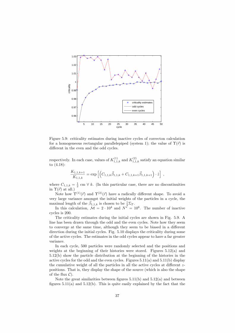
Figure 5.9: criticality estimates during inactive cycles of correcton calculationfor a homogeneous rectangular parallelepiped (system 1); the value of Υ(~r) isdifferent in the even and the odd cycles.

respectively. In each case, values of K(1)1,1,k and K

(2)1,1,k satisfy an equation similar

to (4.18):

K1,1,k+1

K1,1,k= exp

[(C1,1,k

~β1,1,k + C1,1,k+1~β1,1,k+1

)· z]

,

where C1,1,k = 12 cm ∀ k. (In this particular case, there are no discontinuities

in Υ(~r) at all.)Note how Υ(1)(~r) and Υ(2)(~r) have a radically different shape. To avoid a

very large variance amongst the initial weights of the particles in a cycle, themaximal length of the ~β1,1,k is chosen to be 1

2ΣT .In this calculation, M = 2 · 104 and N∗ = 106. The number of inactive

cycles is 200.The criticality estimates during the initial cycles are shown in Fig. 5.9. A

line has been drawn through the odd and the even cycles. Note how they seemto converge at the same time, although they seem to be biased in a differentdirection during the initial cycles. Fig. 5.10 displays the criticality during someof the active cycles. The estimates in the odd cycles appear to have a far greatervariance.

In each cycle, 500 particles were randomly selected and the positions andweights at the beginning of their histories were stored. Figures 5.12(a) and5.12(b) show the particle distribution at the beginning of the histories in theactive cycles for the odd and the even cycles. Figures 5.11(a) and 5.11(b) displaythe cumulative weight of all the particles in all the active cycles at different z-positions. That is, they display the shape of the source (which is also the shapeof the flux C).

Note the great similarities between figures 5.11(b) and 5.12(a) and betweenfigures 5.11(a) and 5.12(b). This is quite easily explained by the fact that the

37

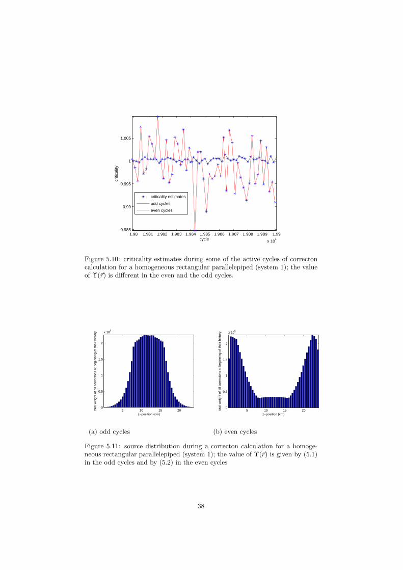
1.98 1.981 1.982 1.983 1.984 1.985 1.986 1.987 1.988 1.989 1.99

x 104

0.985

0.99

0.995

1

1.005

cycle

criti

calit

y

criticality estimates

odd cycles

even cycles

Figure 5.10: criticality estimates during some of the active cycles of correctoncalculation for a homogeneous rectangular parallelepiped (system 1); the valueof Υ(~r) is different in the even and the odd cycles.

5 10 15 200

0.5

1

1.5

2

x 105

z−position (cm)

tota

l wei

ght o

f all

corr

ecto

ns a

t beg

inni

ng o

f the

ir hi

stor

y

5 10 15 200

0.5

1

1.5

2

x 105

z−position (cm)

tota

l wei

ght o

f all

corr

ecto

ns a

t beg

inni

ng o

f the

ir hi

stor

y

(a) odd cycles (b) even cycles

Figure 5.11: source distribution during a correcton calculation for a homoge-neous rectangular parallelepiped (system 1); the value of Υ(~r) is given by (5.1)in the odd cycles and by (5.2) in the even cycles

38

5 10 15 200

2

4

6

8

10

x 104

z−position (cm)

tota

l # p

artic

les

5 10 15 200

2

4

6

8

10

x 104

z−position (cm)

tota

l # p

artic

les

(a) odd cycles (b) even cycles

Figure 5.12: particle distribution during a correcton calculation for a homoge-neous rectangular parallelepiped (system 1); the value of Υ(~r) is given by (5.1)in the odd cycles and by (5.2) in the even cycles

particle distribution in an odd cycle is the result of a source distribution in aneven cycle, and vice versa.

The difference in the variance of the criticality estimates can be accountedfor by comparing the particle distributions (figures 5.12(a) and 5.12(b)). In theodd cycles, far more particles are situated near the edges of the medium andleak out of the system.

The criticality estimates are k = 1.0001456 on average. The error can beestimated based on the odd or the even cycles, leading to 4.8 ·10−5 and 5.8 ·10−6

respectively. This is consistent with the previously found values.Note how the correctons have a completely different flux in every new cycle,

yet the source seems to converge in about the same amount of cycles as in aneutron calculation. Apparently, the method of changing particle weights at thebeginning of their history is very robust.

5.1.3 Real time flux estimation

The real time flux estimation methods proposed in sections 4.3, 4.4 and 4.5 areimplemented for system 1. The system was divided into cubes with ribs of 1cm, so there are 10 cells in the x-direction, 20 cells in the y-direction and 24cells in the z-direction.

The neutron surface fluxes are determined in every cycle. In calculating theparameters for Υ (~r) after cycle j, the average values of the surface fluxes overthe last min (j,H) cycles are used. If there is some surface for which there havebeen no tallies in the last min (j,H) cycles, the calculation of Υ (~r) is skipped.

Using equations similar to 4.16, the value of maxm(a, b, c→ e, d, f) is alsodetermined after every cycle and Υ(~r) is only altered if maxm is below somepreset constant G.

At the beginning of every cycle, the total weight of the particles is normalisedto N∗.

The parameters are H = 20, G = 200,M = 2 · 104 and N∗ = 106. Fig. 5.13

39

50 100 150 200 250 300 350 400 450 500 5501.5

2

2.5

3

3.5

4

4.5

5

cycle

max

[m]

Figure 5.13: typical development of maxm during some of the cycles of cor-recton calculation with real time neutron flux estimation for a homogeneousrectangular parallelepiped (system 1)

is a plot of the development of maxm during some of the cycles. The valuedoesn’t exceed 8.6 in any of the cycles. Υ (~r) is therefore changed in every cycle.

The criticality estimate is k = 1.000461± 1.7 · 10−5 with 100 inactive cycles.In every cycle, 1500 particles were randomly selected and there position and

weight was stored. From this, the source distribution in the active cycles wasobtained. The source as a function of z only is shown in Fig. 5.14. The plotsare very similar when the source is taken as a function of x or y only.

It can be seen that the source (and thus the flux) is almost constant, but itis a little greater near the edges of the medium. This probably indicates a veryslight error in determining the correct Ki,j,k. It could be that an Υ (~r) in theform of Eq. (4.9) is less suitable to describe the neutron flux near the edges ofthe system.

Remember that this does not pose a serious problem, since the choice ofΥ (~r) should not introduce a bias in the calculation (unless it is chosen in suchan unfortunate way that the source iteration becomes unstable).

5.2 System 2: homogenised, loosely coupled fuelassemblies

5.2.1 Basic neutron calculation

A basic neutron calculation has also been performed for the second system.There were M = 1.2 · 104 cycles and N∗ = 105 histories per cycle. A plotof the criticality estimations is shown in Fig. 5.15. It seems to converge afterroughly 50 cycles. Fig. 5.16 shows how the criticality estimates are more or lessconstant during the active cycles. If the number of inactive cycles is taken tobe 200, the average is k = 0.9283358 and the standard deviation of the averageof the criticality estimates is 8.8 · 10−6.

If, however, the source distribution plotted versus the cycles, it becomesapparent that the source doesn’t converge at all. After each cycle, 500 particles

40

2 4 6 8 10 12 14 16 18 20 220

2

4

6

8

10

12

x 105

z−position (cm)

tota

l wei

ght o

f all

corr

ecto

ns a

t beg

inni

ng o

f the

ir hi

stor

y

Figure 5.14: source distribution during the active cycles of correcton calcu-lation with real time neutron flux estimation for a homogeneous rectangularparallelepiped (system 1)

0 10 20 30 40 50 60 70 800.87

0.88

0.89

0.9

0.91

0.92

0.93

cycle

criti

calit

y

Figure 5.15: criticality estimates during inactive cycles of neutron calculationfor loosely coupled fuel assemblies (system 2)

41

2000 3000 4000 5000 6000 7000 8000 9000 10000 11000

0.9282

0.9282

0.9283

0.9283

0.9284

0.9284

cycle

criti

calit

y

Figure 5.16: criticality estimates during some active cycles of neutron calcu-lation for loosely coupled fuel assemblies (system 2) (smoothed with Savitzky-Golay filter of order 103)

were randomly selected and their positions were stored. Fig. 5.17 shows thenumber of particles in the different fuel assemblies versus the cycles. After500 cycles, hardly any of the neutrons are present in the third and fourth fuelassembly. Even after many thousands of cycles, the source distribution is stillaltering in the other fuel assemblies.

The simulation has been repeated 6 times with M = 3 · 103 cycles. In eachcase, fuel assemblies 3 and 4 were quickly left with almost no neutrons. In someof the simulations, some of the other fuel assemblies emptied as well.

At first sight, it may seem strange that the neutrons have a tendency to pileup in the outer parts of the system. This is explained by the fact that the outerfuel assemblies (1,2,5 and 6) are surrounded by more concrete than the innerones. Concrete has a much higher value of Σs/Σa. Therefore, neutrons thatleak out of the fuel assembly have a higher probability of scattering back intothe fuel.

It is interesting how the criticality estimate was consistently approximatelyk = 0.9283 throughout all realisations. Apparently it doesn’t matter wherethe neutrons are in a criticality calculation. This is probably because the fuelassemblies are all equally shaped.

5.2.2 Real time flux estimation

A calculation similar to the one of section 5.1.3 has been done for the looselycoupled fuel assemblies of system 2. The number of cells in the x-, y- andz-direction are 8, 5 and 3 respectively. They are bounded by the planes x =0, 40, 70, 100, 115, 130, 160, 190, 230, y = 0, 40, 80, 120, 160, 200 and z = 0, 20, 100, 120(all values in cm.). This means that the outer fuel pins (1,2,5 and 6) consist ofonly one cell, whilst the inner fuel pins (3 and 4) consist of two equally shaped

42

1000 2000 3000 4000 5000 6000 7000 8000 9000 10000 11000 12000

20

40

60

80

100

120

140

160

180

200

220

cycle

num

ber

of p

artil

ces

at b

egin

ning

his

tory

(i.e

.: th

e so

urce

)

fuel assembly 1

fuel assembly 2

fuel assembly 3

fuel assembly 4

fuel assembly 5

fuel assembly 6

Figure 5.17: positions of 500 randomly selected particles at the beginning oftheir history in loosely coupled fuel assemblies (system 2), versus some of theactive cycles (smoothed with moving average filter of order 80)

43

500 1000 1500 2000 2500 3000 3500

0.8

1

1.2

1.4

1.6

1.8

2

x 105

cycle

tota

l wei

ght o

f all

corr

ecto

ns a

t beg

inni

ng o

f the

ir hi

stor

y

fuel assembly 1

fuel assembly 2

fuel assembly 3

fuel assembly 4

fuel assembly 5

fuel assembly 6

Figure 5.18: total weight of 1500 randomly selected particles at the beginningof their history versus some of the active cycles (smoothed with moving aver-age filter of order 80) for the real time flux estimation of loosely coupled fuelassemblies (system 2)

cells that are located at different x-positions.This time, the parameters were H = 100, G = 200, M = 4 · 103 and

N∗ = 106. The calculation has been done three times; the results were verysimilar in every respect.

The number of inactive cycles is 100; the criticality estimate is k = 0.928217±2.8 · 10−5.

In every cycle, 1500 particles were randomly selected and their properties atthe beginning of their history were stored. The total weight of all particles in afuel assembly is plotted in Fig. 5.18.

Fig. 5.19 is a plot of maxm versus the cycle.Since all fuel assemblies are of the same size, Fig. 5.18 clearly shows that

the source, and thus also the flux, are far from homogeneous. However, thereis a definite improvement over the conventional neutron calculation (Fig. 5.17).The inner fuel assemblies are not completely drained off particles and the outerfuel assemblies have a (more or less) constant source term.

Apparently, the real time flux estimation compensates to a significant de-gree for the destabilisation of the source convergence. This is quite a remarkableachievement, considering the fact that the fuel assemblies are separated by ap-proximately a hundred mean free paths of a neutron.

The most probable explanation for the spatial variance in the correctonsource is that there still aren’t enough particles that can travel from the outerto the inner fuel assemblies to compensate for the difference in the multiplicationfactor.2

2For an alternative explanation, observe that the total correcton source in a fuel assembly

44

500 1000 1500 2000 2500 3000 3500 4000

15

20

25

30

35

40

45

50

cycle

max

[m]

Figure 5.19: maxm for all cycles of the real time flux estimation of looselycoupled fuel assemblies (system 2)

5.2.2.1 Two-dimensional flux estimation

The problems with source convergence are a result of a lack of communicationbetween particles in the fuel pins in different x- and y-positions. In order forthe source to converge, there is no need to even out the flux distribution in thez-direction.

Therefore, one might expect better results if ~βi,j,k · z ≡ 0, since Eq. (4.10)

puts less of a restriction on ~βi,j,k · x and ~βi,j,k · y. The exact same calculationas above has been performed with a slight modification of Eq. (4.13):

~βi,j,k = min

((ΣT )i,j,k`∗i,j,k

, 1

) ln

(Fi+,j,kFi−,j,k

)2Ai,j,k

,

ln

(Fi,j+,kFi,j−,k

)2Bi,j,k

, 0

T

,

where

`∗i,j,k ≡

√√√√√√√ ln

(Fi+,j,kFi−,j,k

)2Ai,j,k

2

+

ln

(Fi,j+,kFi,j−,k

)2Bi,j,k

2

.

should be proportional to the total correcton flux, which is

∫∫<4π>

∫∫∫fuel assembly

C(~r, Ω

)d~r

dΩ =

∫∫<4π>

∫∫∫fuel assembly

φ(~r, Ω

)Υ (~r)

d~r

dΩ .

The exponential form of Υ (~r) is an extremely bad fit for the neutron flux within a fuelassembly. Therefore, the fact that Ki,j,k was chosen to satisfy Eq. (4.19) is hardly a reasonto believe that the rhs of the equation above will be the same for every fuel assembly (especiallysince the inner fuel assemblies consist of two cells, as opposed to the outer ones).

45

The value of Ki,j,k can be adjusted in a similar manner to the one proposedin section 4.5.2. (Some of the calculations need a slight adjustment, since not

all cartesian components of ~βi,j,k are nonzero.)A test showed no significant difference with the three-dimensional case. In

this particular case, the fuel assemblies consist of only one cell in the z-direction,so Fi,j,2+ ≈ Fi,j,2− and thus ~βi,j,2 · z ≈ 0 anyway.

5.2.2.2 Choice of the cell sizes

The first thing to note about the choice of the cell sizes is that the calculationtime rapidly increases when more cells are used.

With other numerical methods that use grids in mind, it may seem temptingto choose smaller cells in the regions where one would expect a large divergencein the neutron flux (e.g. the boundary of a fuel assembly).

However, the tests from section 5.1.2 imply that this is not necessary toensure source convergence inside a fuel pin, where there are no gabs betweenthe regions where fission can occur. In systems like these, the problem is a lackof particles that travel large distances. To solve this, there is no need to bebothered by the flux distribution within a fuel assembly.

In fact, using smaller cells can easily lead to high discontinuities in Υ, com-pletely destabilising the source convergence. This is mostly because far fewerparticles will cross a small surface of a cell, resulting in large statistical variancesin the estimation of the surface flux. This effect is even stronger if there aresmall cells near the boundary of a fuel assembly, where the neutron flux is lowand its gradient is steep.

In the calculation above, the choice of cells can be adjusted to enhance theconvergence. Because the inner fuel assemblies have two cells in the x-directionand the flux is higher in the centre, the correctons are pushed outward. Thesame calculation has been repeated with only one cell in each of the inner fuelassemblies.

A plot of the resulting total correcton sources in the fuel assemblies (similarto Fig. 5.18) is shown in Fig. 5.20. After some cycles, the total source (andthus the total flux) is equal for all fuel assemblies.

With 900 inactive cycles, the criticality is estimated to be k = 0.928401 ±4.1 · 10−5.

A peculiar detail in the calculation is that the total correcton source in fuelassembly 1 suddenly increases by a factor of 1.5 after cycle 5657. Possibly thereis a single particle that gained a very large weight. The particles gradually evenout again over the next 50 to 100 cycles.

5.3 Other tests

The correcton method has been tested for several systems with loosely coupledfuel assemblies, similar to system 2. For example, in one test the concrete hasbeen made a good absorber, so it doesn’t scatter the particles back into thefuel assemblies. In another simulation, there were more fuel assemblies withless symmetry in the system. Several tests have also been done with a far lowernumber of simulated histories per cycle (in the order of 104).

46

1000 2000 3000 4000 5000 6000 7000 8000 9000

130

140

150

160

170

180

190

cycle

tota

l wei

ght o

f all

corr

ecto

ns a

t beg

inni

ng o

f the

ir hi

stor

y

fuel assembly 1

fuel assembly 2

fuel assembly 3

fuel assembly 4

fuel assembly 5

fuel assembly 6

Figure 5.20: source in different fuel assemblies for a new real time flux estimation(smoothed with moving average filter of order 250); compare with Fig. 5.18

In every case, the correctons converged to a more or less uniform distribution.The method seems to work well, so long as all the fuel assemblies and the spacesin between consist of only one cell.

47

Chapter 6

Conclusion

A self-learning correcton method has the potential of solving some of the sourceconvergence problems present in conventional Monte Carlo calculations. Thegreatly reduced spatial variance of the particle distribution should also makeestimating the flux at different locations in a system simultaneously more effi-cient.

Other advantages include:

• No prior calculations are necessary.

• It is often easy to verify that the source iteration has converged and isn’ttrapped in some local minimum. After convergence, the flux should havehardly any spatial variation.

• As opposed to a (relatively) more conventional correcton calculation, verylittle expertise or physical insight is needed. However, one still has tochoose the grid cells correctly.

When choosing the size of the grid cells, there are several issues to take intoaccount. Although it may seem counter-intuitive, the relative discontinuities inΥ (~r) are smaller if larger cells are used. This is mostly because there are moreparticles crossing a cell boundary, resulting in more accurate estimations of theaverage flux over the boundary. As a general rule of thumb, one should not betoo bothered by the specific shape of the neutron flux within a fuel assembly.The correctons only have to directed on a larger scale, in such a way that thereis as much interaction as possible between loosely coupled systems.

The choice of Ki,j,k from section 4.5.2 seems to work quite well. Fig. 5.19seems to suggest that the discontinuities in the flux estimate are not particularlytroublesome. A noticeable deviation from a constant flux is visible in Fig. 5.14,but since it is very small, it can simply be ignored.

48

Chapter 7

Future work

The logical next step is to implement a real time flux estimation technique in acommercial Monte Carlo code that either has problems with source convergence,or where the flux has to be estimated in different regions of a system. (This hasnever been done for the correcton method in general.) This will require severalgeneralisations, such as particles that can have any energy and delayed neutrons.

There are also some possible refinements to the methods described here,some of which are listed below.

• The flux estimate during a calculation is based on tallies from some of thelast cycles, where each cycle has been given an equal weight. The sourcemight converge faster if they are weighted and tallies from later cycles aregiven a greater weight.

• The correcton method in general remains untested for a more generalthree-dimensional geometry, where not all cells are rectangular paral-lelepipeds. This will probably make it more difficult to find a good wayto adjust the parameters of the neutron flux estimate.

• In this thesis, attention has only been paid to the maximal theoreticallypossible weight change for a particle that crosses from one cell to an-other. This is a rather crude measure. For example, the region with alarge relative discontinuity in Υ (~r) might well be quite small, thus hardlyendangering the stability of the calculation.

It might also be interesting to investigate how the correlation between es-timates of quantities in different cycles is effected by the real time correctonmethod. It could be that the positions of the particles are less positively cor-related, especially if the neutron flux estimate is based only on the last cycle.This could make it easier to determine the error in the final estimate of thequantity.

49

Appendix A

Notes on stochastics

A.1 Probability and random variables

Intuitively, a stochastic variable is a variable whose value cannot be determinedin advance. The mathematical formalisation of this concept requires the notionof a probability space (O,H,P), which is defined by the following proper-ties. (Kroese et. al. [9], 605-606)

1. O is the set of all possible values of the stochastic variable, called thesample space.

2. H is the σ-field of all events. An event is a subset of O to which aprobability can be assigned. A σ-field H is a collection that satisfies thefollowing properties:

(a) H 6= ∅;(b) A1, A2, . . . ∈ H ⇒ (A1 ∪A2 ∪ . . .) ∈ H;

(c) A ∈ H ⇒ Ac ∈ H.

3. P is a probability measure that assigns a number P(A) to every A ∈ H.It must satisfy the Kolmogorov axioms1:

(a) nonnegativety: P(A) ≥ 0 ∀ A ∈ H;

(b) unit measure: P(O) = 1;

(c) sum rule: Ai ∩Aj = ∅ ∀ i, j ⇒ P(⋃xAx

)=∑xP(Ax).

P(A) is said to be the probability of A.

An event A happens almost surely if and only if P(A) = 1.2

1Sometimes the more intuitive Cox’s theorems are used instead, but they make argumentthat transforms equation (3.8) in section 3.2 into a Markov process more difficult.

2This terminology is used when there are several theoretical outcomes, but only one ofthem doesn’t have a vanishingly small probability. (For example, when tossing a coin 10100

times, there’s a probability of(12

)(10100)that none of the tosses will be a tails. But when the

coin is tossed an infinite number of times, there will almost surely be a tails at least once.)

50

Formally, a stochastic variable X that takes on values in some set E (calledthe state space) is a function X : O → E such that

X ∈ B ≡ γ ∈ O|X(γ) ∈ B ∈ H ∀ B ∈ E , (A.1)

where E is a σ-field on E. If E is countable, then X is called discrete, otherwiseit’s called continuous. (Kroese et. al. [9], 607-609)

Somewhat heuristically, the probability distribution is a function thatdescribes the probability that X ∈ B for all B. If X and Y are stochasticvariables, the statement ‘X ∼ Y ’ denotes that X has the same probabilitydistribution as Y . If X is defined by (A.1) on a well-defined probability space,then all the usual properties of its probability distribution will hold.

Define the probability operator P[−] as follows:

• If S is a statement, P[S] is the probability that S is true.

• If D is a discrete stochastic variable (that is, if E is countable), thenP[D](z) ≡ P[D = z].

• If C is a continuous stochastic variable in the hyperspace Rn, then P[C](z) ≡V −1P[z ∈ V], where z ∈ Rn, V is some vanishingly small part of Rn aboutz and V is the volume of V.

In the last case, P[C] is the probability density function of C. If X cantake on values in the uncountable set Rn, it is quite possible that P(X = α) =0 ∀ α ∈ Rn, whilst not violating the unit measure Kolmogorov axiom. However,the probability density will in general still be positive. From the Kolmogorovaxioms it follows that P[C] ∈ R+ and

∫Rn

dz P[C](z) = 1.

A.2 Markov chains and MCMC

A set J is called an index set of A if there is a surjective function from J toA. A stochastic process is a set of random variables Xτ on a probabilityspace (O,H,P) where τ is in any index set J . It is often helpful to view τ asthe time and Xτ as a random variable that is evolving through time.

A Markov process is a stochastic process that satisfies the Markov prop-erty:

(Xt+s|Xu, u ≤ t) ∼ (Xt+s|Xu, u = t) ∀ s ≥ 0 .3

The Markov property is sometimes called ‘memorylessness’. In words, it canbe interpreted as a stochastic process for which, conditional on its ‘present’state, the ‘past’ and the ‘future’ are independent.

In this thesis, only processes with the index set N are considered. Since theindex set is countable, the process is called a Markov chain. The state spacewill be in Rn.

The transition kernel Ps is a function defined as

Ps(x,A) = P[Xt+s ∈ A|Xt = x] .

3Note this is a conditional probability density. (ref. Dekking et al. [7], chapter 3 orKroese et al. [9], pages 618-619))

51

It is the probability that Xt will ‘evolve’ from x to some value in A in s timesteps. It can usually be written as

Ps(x,A) =

∫A

ps(x, y) dy,

where ps(x, y) is the transition density. All Markov processes will be consid-ered to be time-homogeneous, meaning that the transition kernel, and thusthe transition density, do not depend on the time. (Kroese et. al. [9], 628)

The product rule for probabilities leads directly to the Chapman-Kolmogorovequations:

pa+b(x, y) =

∫q∈E

pa(q, y) pb(x, q) dq .

Also, if f0 is the joint probability density function4 of some Markov chain(R0, R1, . . . , Rn), then

fn(r0, r1, . . . , rn) = f0

n−1∏i=1

p1(rn, rn+1) .

If certain requirements are met (Kroese et. al. [9], 630-635), there will be alimiting distribution π such that

limt→∞

pt(x, y) = π(y) . (A.2)

Under certain conditions, existence of the limiting distribution implies its unique-ness and it can be determined as the solution to the set of equations

π(y) =

∫π(x)ps(x, y) dx ∀ s ∈ N , (A.3)∫

π(y) dy = 1 .

In other words, π is the stationary distribution of the Markov chain.

In a Monte Carlo calculation, it may often be difficult to sample from aprobability distribution f if it cannot be written in a closed form. Though itmay seem surprising, it is often still possible to find some time-homogeneousMarkov chain of which it is known that it has f as its stationary distribution.The transition kernel of this Markov process for a unit time step is usually quitesimple to sample from.

The goal of the Markov chain Monte Carlo (MCMC) method is togenerate approximate samples from some stationary distribution π in Eq. (A.2).This can be done using the power method. To this end, pick some startingvalue X0 and use the unit time step transition kernels to generate a Markovprocess X0, X1, . . .. The idea is that, for some M > 0, XM will have a similarprobability distribution as π. It can thus be used to draw an approximatesample from π.

4ref. Dekking et al. [7], chapter 9

52

Appendix B

Sampling stochasticvariables

B.1 Pseudorandom numbers

A computer program performs a set of prescribed actions. It is incapable ofdoing something at random. For Monte Carlo calculations however, it is nec-essary to sample random variables. To facilitate this, modern programminglanguages are equipped with an algorithm to sample pseudorandom numbersfrom a uniform distribution from 0 to 1. The algorithm generates a sequence ofnumbers that approximates the properties of random variables. The sequenceisn’t truly random, but is determined by a (small) set of variables (the seed)that has to be specified. The seed should be chosen at random.

Since a computer can only store a finite amount of unique variables in the set(0, 1), the sequence of pseudorandom numbers will be repetitive. The periodlength is the largest number of samples that can be drawn from a pseudorandomnumber generator without the guarantee that the sequence is repetitive.

For a more formal discussion of random number generation, the reader isreferred to Kroese, et al. [9], chapter 1. A few basic requirements for ran-dom number generators are also stated there. Amongst others, they shouldnot return the values 0 or 1 and the stream of pseudorandom numbers shouldbe reproducible. Also, the period length should at least be of the order ofmax(1050, 10N2), where N is the number of generated numbers. Most olderrandom number generators didn’t meet this last demand.

For the calculations in this thesis, the seed was sometimes chosen in sucha way that the results are reproducible. In other occasions it was based onthe CPU-time of the computer at the start of the calculation. The period afterwhich the pseudorandom sequence repeats itself is considered to be large enoughto avoid practical problems. The random number generator is assumed to workperfectly.

53

B.2 Sampling from a known probability density

A computer will usually only sample from a uniform distribution from 0 to 1.The following procedure can be used to sample values of a random variable Xwith an arbitrary probability density function f(z). (To see why this works, aplot of a random cumulative probability density function should suffice. See,for instance, Dekking et al. [7], pages 72-73.)

Determine

P [X < z] = F (z) ≡∫ z

−∞f(s)ds (B.1)

and note that F (z) is monotonically increasing function of z and 0 ≤ F ≤ 1.Now define F−1 as the inverse of F .1 Suppose a uniformly distributed randomnumber ρ ∈ (0, 1) has been obtained. If the random variable k is defined by

k = F−1(ρ),

it has a probability density function of f .For example, Eq. (3.9) can be found by taking f to be equal to the expo-

nential distribution of Eq. (2.3). Then, from Eq. (B.1), F (d) = 1− exp (−ΣT d)and thus F−1(ρ) = − 1

ΣTln (1− ρ). Finally, observe that (1− ρ) ∼ ρ.

Discrete random variables can be viewed as continuous variables with aprobability density function that consists of a train of Dirac delta functionsδ. Specifically, if a stochastic variable Y has the possible values y1, y2, . . . , yNwith respective probabilities p1, p2, . . . , pN such that y1 < y2 < . . . < yN , thenit can be treated as a continuous stochastic variable with a probability densityfunction

P [Y ] (u) =

N∑i=1

pi δ(u− yi).

Thus the cumulative probability density function is

P [Y < u] =

∫ u

−∞P [Y ] (s) ds =

N∑i=1

pi H(u− yi),

where H is the Heaviside function. The inverse can easily be determined graph-ically and this leads to the result that Y can be sampled by

y1 +

N−1∑i=1

(yi+1 − yi) H

ρ− i∑j=1

pj

.

(Again, ρ is a uniformly distributed stochastic variable.)An application of this procedure would be to sample the amount of new

neutrons after a fission reaction.One can also randomly select events by attributing a unique number to each

event and following the procedure for sampling discrete stochastic variables.

1F (z) may not be strictly monotonically increasing for all z. On those parts of the domainwhere it isn’t, F−1(z) may not be unambiguously defined, but this is not a problem.

54

Sometimes the methods described above can be very difficult or computa-tionally expensive. Kroese et al. [9], 85-224, provides the most efficient algo-rithms to sample from most well-known probability densities. They are usuallybased on some specific characteristics of the distributions.

B.3 Sampling an isotropic direction vector

If a unit vector Ω is placed at the origin, it will point to some point on the surfaceof the unit sphere around the origin. If it has a random isotropic direction, theprobability that it will point to some part of the surface is proportional to thearea of that part of the surface. Define the Cartesian coordinates x, y and z andΩi ≡ Ω · i ∀ i ∈ x, y, z. The probability that z < Ωz < z + dz is proportionalto the area of a unit sphere between z and z + dz.

This area can be calculated as the ‘rotational area’2 of the function y =√1− z2 about the z-axis. In general, the length of a surjective function y = y(x)

between x and x+ dx is√dx2 + dy2 =

√1 + (y′(x))

2dx .

Putting everything together,

P [z < Ωz < z + dz] =

(2π ·√

1− z2)(√

1 +(

ddz

(√1− z2

))2dz

)(total area of the unit sphere)

=1

2dz

for all z ∈ (−1, 1).Using spherical coordinates and denoting the polar and azimuth angles by

ϑ and γ, any book on calculus will tell you that

(Ωx, Ωy, Ωz) = (sinϑ cosγ, sinϑ sinγ, cosϑ) . (B.2)

Therefore cosϑ can be sampled from a uniform distribution from −1 to 1. Be-cause of symmetry, it is obvious that γ has a constant probability density func-tion with a width of 2π.

Using Eq. (B.2) in combination with some trigonometric identities, thecartesian components of an isotropic unit vector can now be sampled by

Ωx = 2√ζ1 (1− ζ1) cos(2πζ2),

Ωy = 2√ζ1 (1− ζ1) sin(2πζ2),

Ωz = 2ζ1 − 1,

where ζ1 and ζ2 are independent and uniformly distributed from 0 to 1.

2the area of the surface of the solid that is generated by revolving a function around anaxis

55

Appendix C

System specifications

C.1 System 1: simple bar

This system consists of a homogeneous rectangular parallelepiped in an infinitevacuum. If x, y and z are the cartesian coordinates, then the bar is boundedby the planes x, y, z = 0 cm, x = 10 cm, y = 20 cm and z = 24 cm. Themacroscopic cross sections are ΣT = 1.0000 cm−1, Σa = 0.5882 cm−1 andΣf = 0.2500 cm−1. The average number of new neutrons produced in a fissionreaction is ν = 2.5.

The system is very nearly critical.

C.2 System 2: fuel assembly # 1

The system consists of a rectangular parallelepiped medium surrounded by aninfinite vacuum. Denote the cartesian coordinates by x, y and z and take oneof the corners of the parallelepiped to be the origin. Define the length l ≡ 1 cmand x∗ ≡ x/l, y∗ ≡ y/l and z∗ ≡ z/l.

The medium consists of three different materials: water, concrete and sixequally shaped fuel assemblies. Let F , W and C be the regions where there isfuel, water or concrete respectively. The ith fuel assembly is in Fi.

The composition of the medium is given by

F1 ≡ x, y, z ∈ R3| 040 < x∗ < 070 ∧ 040 < y∗ < 080 ∧ 020 < z∗ < 100 ;

F2 ≡ x, y, z ∈ R3| 040 < x∗ < 070 ∧ 120 < y∗ < 160 ∧ 020 < z∗ < 100 ;

F3 ≡ x, y, z ∈ R3| 100 < x∗ < 130 ∧ 040 < y∗ < 080 ∧ 020 < z∗ < 100 ;

F4 ≡ x, y, z ∈ R3| 100 < x∗ < 130 ∧ 120 < y∗ < 160 ∧ 020 < z∗ < 100 ;

F5 ≡ x, y, z ∈ R3| 160 < x∗ < 190 ∧ 040 < y∗ < 080 ∧ 020 < z∗ < 100 ;

F6 ≡ x, y, z ∈ R3| 160 < x∗ < 190 ∧ 120 < y∗ < 160 ∧ 020 < z∗ < 100 ,

F = F1 ∪ F2 ∪ F3 ∪ F4 ∪ F5 ∪ F6 ,

W = x∗, y∗, z∗ ∈ R3|40 < x∗ < 190 ∧ 40 < y∗ < 160 ∧ 20 < z∗ < 100 \ F

56

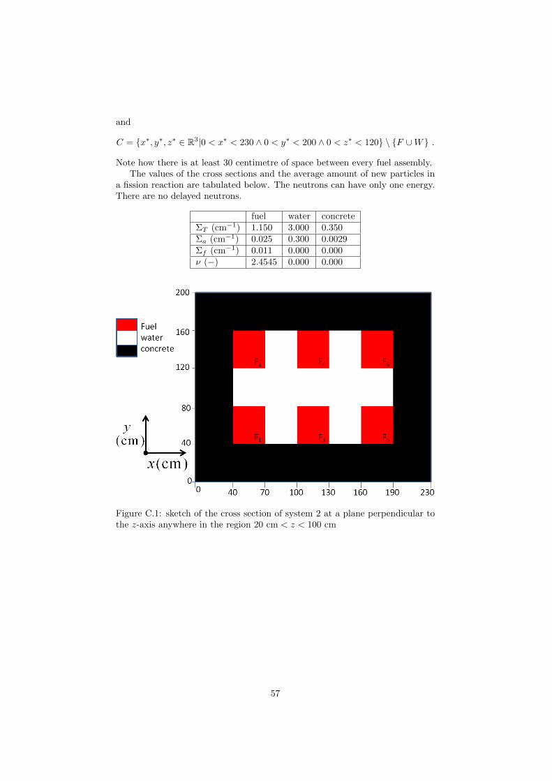
and

C = x∗, y∗, z∗ ∈ R3|0 < x∗ < 230 ∧ 0 < y∗ < 200 ∧ 0 < z∗ < 120 \ F ∪W .

Note how there is at least 30 centimetre of space between every fuel assembly.The values of the cross sections and the average amount of new particles in

a fission reaction are tabulated below. The neutrons can have only one energy.There are no delayed neutrons.

fuel water concreteΣT (cm−1) 1.150 3.000 0.350Σa (cm−1) 0.025 0.300 0.0029Σf (cm−1) 0.011 0.000 0.000ν (−) 2.4545 0.000 0.000

Figure C.1: sketch of the cross section of system 2 at a plane perpendicular tothe z-axis anywhere in the region 20 cm < z < 100 cm

57

Bibliography

[1] Hoogenboom, J. E., Sjenitzer, B. L.: Monte Carlo Lectures, PNR, R3,TNW, TU Delft (2011)

[2] Duderstadt, J. J., Hamilton, L. J.: Nuclear Reactor Analysis, Wiley (1976),Department of Nuclear Engineering, The University of Michigan

[3] Bowler, M. G.: Nuclear Physics, Pergamon Press (1973)

[4] Sjenitzer, B.: Variance Reduction Using The Correcton Method on Criti-cality Calculations, TU Delft, PNR (2009)

[5] Becker, T. L., Wollaber, A., B., Larsen, E. W.: A Hybrid Monte Carlo-Deterministic Method for Global Particle Transport Calculations, Univer-sity of Michigan, Department of Nuclear Engineering and Radiological Sci-ences (2006)

[6] Becker, T, L.: Hybrid Monte Carlo/Deterministic Methods for RadiationShielding Problems, Nuclear Engineering and Radiological Sciences, Uni-versity of Michigan (2009)

[7] Dekking, F. M., Kraaikamp, C., Lopuhaa, H. P., Meester, L. E.: A ModernIntroduction to Probability and Statistics, Understanding Why and How,Springer texts in statistics (2009), applied mathematics, TU Delft

[8] Huisman, M., V.: variance reduction in a three dimensional space using thecorrecton method, TU Delft, PNR (2011)

[9] Kroese, D. P., Taimre, T., Botev, Z. I.: Handbook of Monte Carlo Methods,Wiley series in probability and statistics (2011)

58