corporate tax cuts and foreign direct...
TRANSCRIPT

CORPORATE TAX CUTS AND FOREIGN DIRECT INVESTMENT
Leonardo Baccini, Quan Li, and Irina Mirkina
Abstract
Accurate policy evaluation is central to optimal policymaking, but difficult to achieve.Most often, analysts have to work with observational data and cannot directly observethe counterfactual of a policy to assess its effect accurately. In this paper, we crafta quasi-experimental design and apply two relatively new methods—the difference-in-differences estimation and the synthetic controls method—to the policy debate onwhether corporate tax cuts increase foreign direct investment (FDI). The taxation–FDI relationship has attracted wide attention because of mixed findings. We exploita quasi-experimental design for Russian regions, which were granted autonomy toreduce corporate profit tax in 2003, enabling them to simultaneously experiment withdifferent tax policies. We estimate both the average and local treatment effects of twotypes of tax cuts on FDI inflows. We find that, on average, relative to the absenceof tax cuts, nondiscriminatory tax cuts on direct investment profit increase FDI, butdiscriminatory tax cuts on selected government-sanctioned investment projects do not.Yet for both types of tax cuts, local treatment effects vary dramatically from region toregion. Our research has important implications for the design of tax policy and fiscalincentive, and the assessment of fiscal policy reforms. C© 2014 by the Association forPublic Policy Analysis and Management.
INTRODUCTION
Accurate policy evaluation is central to optimal public policymaking. But evaluat-ing the effect of a policy reliably has always been challenging. The most credibleevaluation is to estimate and compare the effect of a policy between treatmentand control groups in a well-designed experiment, in which the policy is randomlyassigned among subjects such that treated and control groups are identical in allaspects except for the policy treatment. Needless to say, this field experiment ap-proach is not feasible in most real-world policy analyses, in which analysts can-not randomly assign treatments and have to work with observational data, poli-cies are often endogenous and open to the influences of subjects, and treated andcontrol groups are not homogeneous or balanced in many dimensions. Yet policyshocks often offer unique opportunities for credible evaluation. In this paper, wecraft a quasi-experimental design in the context of Russian regional tax reformsand apply two relatively new methods—the difference-in-differences (DID) estima-tion and the synthetic controls method (SCM)—to a widely debated policy issue,that is, the impact of corporate tax cuts on foreign direct investment (FDI). Ouranalysis sheds new light on a longstanding debate of relevance to policymakers,businesses, and scholars in public economics, international business, and politicalscience.
Journal of Policy Analysis and Management, Vol. 33, No. 4, 977–1006 (2014)C© 2014 by the Association for Public Policy Analysis and ManagementPublished by Wiley Periodicals, Inc. View this article online at wileyonlinelibrary.com/journal/pamDOI:10.1002/pam.21786

978 / Corporate Tax Cuts and Foreign Direct Investment
In the past several decades, many governments at national and subnational lev-els in Europe, America, and Asia sought to attract FDI by setting up investmentpromotion agencies and offering various fiscal incentives (Li, 2006; OECD, 2003a;UNCTAD, 2000). While policymakers believed tax incentives helped to attract FDI,multinational enterprise (MNE) managers provided more heterogeneous survey re-sponses, and many did not rank taxes as very important for investment decisions(Tavares-Lehmann, Coelho, & Lehmann, 2012). Such incongruence in belief andperception between policymakers and managers is puzzling. Further adding confu-sion to the puzzle, empirical studies from the 1950s to the 1990s produced mixedfindings and yet in the past decade and a half, most, though not all, econometricstudies appeared to show that lower tax rates encourage more FDI (De Mooij & Ed-erveen, 2003, 2008; Devereux, 2007; Hines, 1996, 1999; Tavares-Lehmann, Coelho,& Lehmann, 2012).
In this paper, we offer an innovative empirical analysis of the question of whethercorporate tax cuts cause more FDI. We address three weaknesses in previous econo-metric studies on this topic. First, most empirical studies focus on national-level taxrates, but in many countries, subnational governments also influence tax rates oncorporate profit and they often adopt different tax policies. Ignoring subnationaldiscretion and distinctions over corporate tax policy leads to measurement errorsand biased estimates. Second, many empirical studies pool together very differentcountries, the unobservable heterogeneity of which tends to bias the estimated ef-fect of taxation. Third, extant econometric studies focus on estimating the averageeffect of taxation and pay insufficient attention to the issue of how to identify andcompare such effect with the counterfactual, that is, the outcome for the same unitin the absence of a tax cut. To address these three weaknesses, we apply a quasi-experimental design and two quasi-experimental methods to a single country whereregional governments were granted autonomy to cut corporate profit tax rates atthe same time.
Russian regions during the 1995 to 2008 period provide an ideal setting for suchan analysis. In 2002, for the first time, the federal government granted regionalauthorities the autonomy to reduce their corporate profit tax rates. In response, re-gional authorities in 82 regions adopted three different corporate profit tax regimes:maintaining the status quo flat rate (no tax cut), tax concession for direct investmentprofit (nondiscriminatory tax cut), and tax concession for profit from government-sanctioned important investment projects only (discriminatory tax cut). The exoge-nously granted policy autonomy allowed the regions to experiment simultaneouslywith different corporate tax policies. This quasi-experimental scenario presents anopportunity to estimate the effects of tax cuts on FDI across regions within a singlecountry over time.
As noted, we apply two quasi-experimental methods: a parametric identificationstrategy based on DID estimation and a nonparametric identification strategy basedon SCM. DID estimates the average treatment effect for the treated units, and SCMidentifies the local treatment effect specific to each region. In our findings, thoseregions that cut taxes on direct investment profit in a nondiscriminatory mannerattract on average significantly more FDI than status quo regions. We also find that,on average, regions that cut tax on investment profit from government-approvedimportant projects do not attract significantly more FDI than status quo regions.Yet for both types of tax cuts, the local treatment effects could vary dramaticallyfrom region to region.
Our research makes several contributions. Substantively, our findings providevaluable knowledge on the taxation–FDI relationship. We identify the type of taxcut that is likely to attract FDI. In addition, we find that the effect of a tax cut,even when it works, often varies among different jurisdictions. Finally, we showthat fiscal autonomy does not always generate preferred economic outcomes. The
Journal of Policy Analysis and Management DOI: 10.1002/pamPublished on behalf of the Association for Public Policy Analysis and Management

Corporate Tax Cuts and Foreign Direct Investment / 979
success of fiscal decentralization often depends on policy design at the regionallevel.
Methodologically, we exploit varying regional responses to the same shock withinthe same country and produce comparisons and inferences based on more ho-mogeneous conditions than those in previous studies. In addition, the two quasi-experimental statistical methods not only allow us to obtain the average treatmenteffects of tax cuts, but also their local treatment effects specific to regions. The latterinformation should be of particular interest to policymakers of individual jurisdic-tions. For researchers, the two methods are easily applicable to other policy issueareas of Tiebout-style sorting and for evaluating policies in federal systems like inour study.
The rest of the paper proceeds as follows. The next section provides a briefoverview of the empirical literature on tax and FDI. The following section discusseswhy Russian regions provide an ideal quasi-experimental setting and examinessome fundamental assumptions underlying our empirical strategy. The next twosections present the parametric DID identification strategy and the associatedresults, followed by two sections that discuss the nonparametric SCM identificationstrategy and the associated results. The final section concludes the paper.
BRIEF LITERATURE REVIEW ON TAXATION AND FDI
FDI refers to the purchase by a MNE of physical assets or a significant portion ofthe ownership (stock) of a company in another country to acquire managementcontrol. It often involves real investment in plants and equipment or financial flowsthrough mergers and acquisitions, resulting in joint ventures or sole ownerships.Different types of FDI may respond to taxes differently (Auerbach & Hassett, 1993;Blonigen & Piger, 2011; Kessing, Konrad, & Kotsogiannis, 2009). In this paper wedo not study variations among different types of FDI, but focus on the aggregateFDI inflows into each region. The literature on tax and MNE activity is too large tofully review here. We provide a brief overview to set the stage for our applicationof the two quasi-experimental methods. Many scholars provide extensive reviews ofdozens of studies on the topic (see, e.g., De Mooij & Ederveen, 2003, 2008; Devereux,2007; Hines, 1996; Tavares-Lehmann, Coelho, & Lehmann, 2012).
In the international business literature, the most widely applied theoretical frame-work for explaining FDI is John Dunning’s eclectic paradigm of international pro-duction. According to Dunning (1988, 1993), international direct investments byMNEs are motivated by three sets of advantages they possess relative to host orother foreign firms not engaged in international production: ownership-specificadvantages, based on their tangible and intangible assets (e.g., capital, productinnovation, management practice, marketing technique, and brand name); inter-nalization advantages, due to their hierarchical control of value-added activities inmultiple countries; and location-specific advantages, resulting from the host coun-try’s resource endowments, economic conditions, and government policies (e.g.,tariff, corporate taxation, investment or tax regulation, profit repatriation or trans-fer pricing, royalties on extracted natural resources, antitrust regulation, technologytransfer requirement, intellectual property protection, or labor market regulation).Taxes could influence all three types of advantages of a foreign firm (De Mooij &Ederveen, 2003, 2008). Since taxes reduce the net returns to any firm, all MNEs pre-fer, though to varying degrees, to pay lower taxes. Theoretically, one should expectlower tax rates to attract more investment inflows. Yet extant empirical evidencetends to be mixed.
Econometric studies typically regress measures of foreign investment on tax vari-able(s) while controlling for other relevant factors. As shown in a number of surveys
Journal of Policy Analysis and Management DOI: 10.1002/pamPublished on behalf of the Association for Public Policy Analysis and Management

980 / Corporate Tax Cuts and Foreign Direct Investment
of the literature noted earlier, these studies differ in various respects. The dependentvariable may be FDI flows, FDI stock, the number of foreign investment locations,or investment in property, plant, and equipment. The tax variables also differ acrossstudies, measured as statutory tax rate, tax base, average tax rate, effective tax rate,effective marginal tax rate, effective average tax rate, or bilateral corporate effectivetax rate. The design could be time series, cross-sectional, or panel, and could beat the firm, industry, subnational, country, or bilateral level. Studies from earlierdecades produce mixed findings on the impact of corporate tax on FDI, but mostrecent research (e.g., Becker, Egger, & Merlo, 2012; Bellak & Leibrecht, 2009; Bel-lak, Leibrecht, & Damijan, 2009; Blonigen & Davies, 2004; Devereux & Griffith,1998; Egger et al., 2009; Grubert & Mutti, 2000, 2004) often finds that corporate taxsignificantly reduces FDI or MNE activities. Yet, conflicting evidence still emerges.For example, using better identification strategies to address tax policy endogene-ity, Jensen (2012) finds that corporate tax rates do not affect FDI inflows in 19industrialized economies from 1980 to 2000.
As noted earlier and by various scholars in the literature, most extant studies tendto focus on national corporate tax rates and pool heterogeneous countries in theirsamples. Only a small number of studies examine the impact of corporate taxes setby subnational governments on FDI. For example, Bartik (1985), Slemrod (1990),Papke (1991), and Hines (1996) examine how state-level corporate income taxesaffect FDI allocation (in terms of investment and plant location) among 50 U.S.states. Swenson (1994) studies how average tax rates affect aggregate FDI inflowsin 18 different industries into 50 U.S. states between 1979 and 1991. Becker, Egger,and Merlo (2012) study the effect of business tax rates by German municipalities onlocation decisions of foreign MNEs.
Beyond the United States and Germany, subnational governments in many othercountries also have autonomy levying taxes on corporations. Thus more research isneeded to study the impact of different types of tax policies of regional governmentson FDI. Focusing on intra-country variations holds constant the unobserved cross-national heterogeneity in terms of endowment, culture, institution, political deci-sionmaking process, and economic structure that tends to bias the estimated effectof taxation, thus eliminating the confounding effect of unobserved cross-nationaldifferences and isolating the effect of interest.
More importantly, extant empirical studies rarely pay attention to designingproper identification strategies before estimation. Many scholars (Abadie, 2005;Abadie, Diamond, & Hainmueller, 2010; Abadie & Gardeazabal, 2003; Angrist &Pischke, 2008; Holland, 1986; Rubin, 1974, 1977) show that regardless of the is-sue area, estimated policy effects based on conventional regression models tendto be unreliable. They argue in favor of various new identification and estima-tion strategies to get at the effect of public policy. In this study, we take advan-tage of recent methods that improve the identification strategy with observationaldata to provide better tests and estimates of the effects of corporate tax cuts onFDI.
EFFECTS OF QUASI-EXPERIMENTAL TAX CUTS ON FDI IN RUSSIAN REGIONS
We analyze whether corporate investment profit tax cuts induce more FDI inflowsinto Russian regions. The outcome variable is the amount of FDI inflows into aRussian region in a given year, measured in thousands of constant 2000 U.S. dol-lars and log transformed. Data are from the Federal Statistic Service of Russia
Journal of Policy Analysis and Management DOI: 10.1002/pamPublished on behalf of the Association for Public Policy Analysis and Management

Corporate Tax Cuts and Foreign Direct Investment / 981
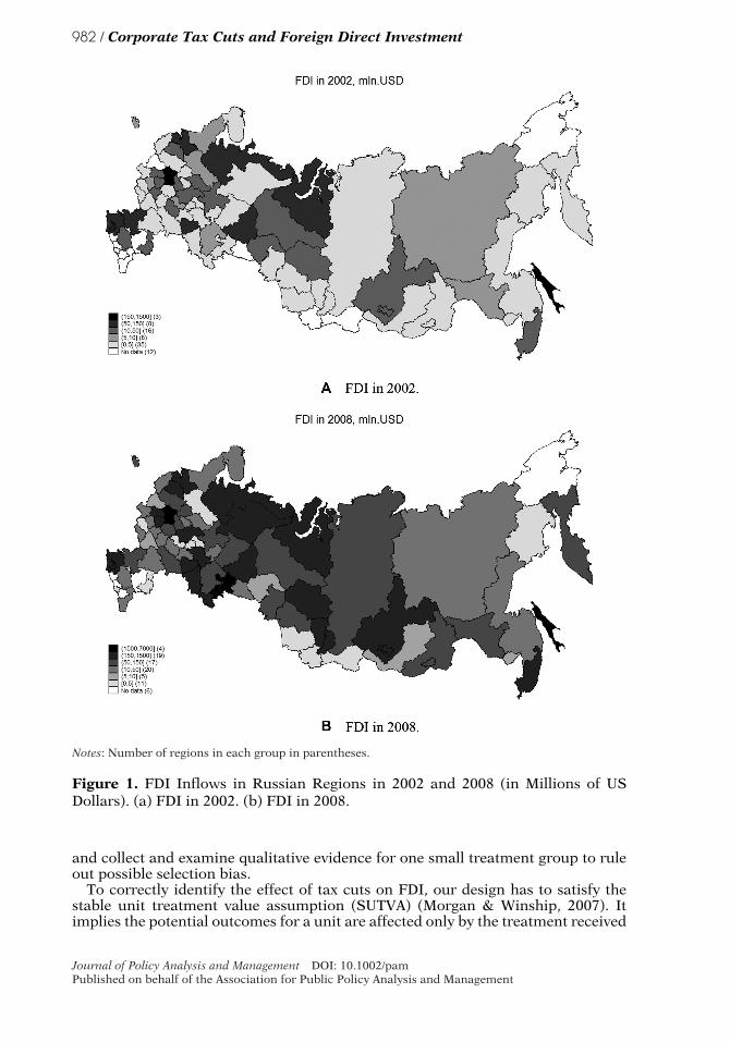
(Rosstat).1 The FDI data reflect a direct-investor ownership of at least 10 percent ofthe ordinary shares in the equity capital of an enterprise residing in Russia by a di-rect investor from a foreign country. Direct investment can be in the form of equitycapital, reinvested earnings, intracompany loans, and financial leasing, but does notinclude investment in monetary institutions or banks (for statistical purposes, thelatter is included in other foreign investment in Rosstat’s data).2 Figure 1 maps theintensity of FDI inflows into 82 Russian regions in 2002 and 2008, showing thatthere are significant variations in FDI flows both across regions and over time.
In our design, the treatment variable is the corporate profit tax cut. As in manyother countries, Russian profit tax is the tax on the income of legal entities, imposedon net annual profit. We choose to study corporate profit tax because it is one of themain sources of regional budget revenues, accounting for 20 to 70 percent of theirnontransferable income. All other types of taxes are either low (hence insignificantfor regional tax revenues) or imposed at the federal level (so that regional authoritiescannot exercise discretion).
As a result of the Tax Code changes in 2002, corporate profit tax cuts in differentRussian regions provide a quasinatural experiment for evaluating the effects of taxcuts on FDI. In Russia, even though corporate profit tax rates always had both afederal and a regional component, setting the rates for both components was tradi-tionally the prerogative of the federal government. However, chapter 25 of the TaxCode, which entered into force in 2002, introduced a new regime for corporate profittax. The regions were given autonomy to reduce their part of the profit tax rate. Withthis newly granted power from the federal government, beginning in 2003, regionalauthorities experimented with three different types of corporate profit tax regimes:maintaining the status quo flat tax rate for corporate profit in general (no tax cut),tax concessions for direct investment profit (hence two separate rates for profit anddirect investment profit, applied in an nondiscriminatory manner), and tax conces-sions for government-sanctioned investment projects only (discriminatory tax cut).No tax cut status quo regions had only one flat tax rate for corporate profit fromall sources. Nondiscriminatory tax cut regions adopted separate tax rates for profitand direct investment profit, cutting the latter to encourage direct investment. Dis-criminatory tax cut regions, like no tax cut regions, implemented one flat rate forcorporate profit, but they selectively reduced tax rates for profit from importantinvestment projects only.
In the absence of a truly randomized policy experiment, we consider our study ofthe observable tax cuts among Russian regions as approximating only a quasinaturalexperiment. The autonomy to reduce corporate profit tax, exogenously imposed bythe federal government, made it possible for regions to experiment with differenttypes of tax policies. Tax cuts, which occurred in some regions but not in othersduring the 2003 to 2008 period, present a great opportunity to study their effects onFDI. The fact that the policy choices of different regions could be endogenous makesthis not a randomized experiment, which is common in policy evaluations. Hencebefore estimating the treatment effects, we take great efforts to design our study torule out various confounding possibilities. As we discuss in detail below, we pickregions for control and treatment groups carefully, test whether they are balancedon a large number of covariates, explore whether endogenous tax cuts as theorizedin an influential study by Cai and Treisman (2005) are present in our sample or not,
1 FDI data are reported by both Rosstat and the Bank of Russia in accordance with the methodology setout by the International Monetary Fund, but only Rosstat offers the data disaggregated by regions.2 Meyer and Pind (1999), and Vinhas de Souza (2008a) address the issue of low reliability of Russianstatistics on FDI in detail. Some methodology comparisons are presented also in OECD (2003b).
Journal of Policy Analysis and Management DOI: 10.1002/pamPublished on behalf of the Association for Public Policy Analysis and Management
982 / Corporate Tax Cuts and Foreign Direct Investment
Notes: Number of regions in each group in parentheses.
Figure 1. FDI Inflows in Russian Regions in 2002 and 2008 (in Millions of USDollars). (a) FDI in 2002. (b) FDI in 2008.
and collect and examine qualitative evidence for one small treatment group to ruleout possible selection bias.
To correctly identify the effect of tax cuts on FDI, our design has to satisfy thestable unit treatment value assumption (SUTVA) (Morgan & Winship, 2007). Itimplies the potential outcomes for a unit are affected only by the treatment received
Journal of Policy Analysis and Management DOI: 10.1002/pamPublished on behalf of the Association for Public Policy Analysis and Management
Corporate Tax Cuts and Foreign Direct Investment / 983
by that unit. No interference occurs between units. Spillover and contagion effectsviolate this assumption. Thus, we design our control and treatment groups carefullyto meet SUTVA. The control group includes those regions that implemented no taxcuts and kept the tax rate on profit from direct investment unchanged at 24 percentfrom 2002 to 2008. This group contains 36 regions.
The first treatment tax regime is applied in 10 nondiscriminatory tax cut regions.An investor in such a region was eligible for the reduced tax rate for net incomereceived from direct investment. Based on the timing of tax cut, we separate the 10regions into two groups: nondiscriminatory tax cut1 and nondiscriminatory tax cut2.Seven nondiscriminatory tax cut1 regions passed legislation on tax code changes in2003, as soon as they were able to do so, and implemented them in 2004, reducingtheir tax rates on direct investment profit to 20 percent (two regions) or 20.5 percent(five regions). Three nondiscriminatory tax cut2 regions passed and implementedsimilar legislations in subsequent years (2004 and 2005). Since subsequent tax cutsin those tax cut2 regions were likely influenced by others, thus violating SUTVA,we only estimate the difference between no tax cut and nondiscriminatory tax cut1regions. In addition, we could not find FDI data for the Kalmykia Republic in thenondiscriminatory tax cut1 group and excluded it from analysis. Appendix Table A1lists specific regions and their respective tax change legislations.3
The second treatment tax regime is applied in 34 discriminatory tax cut regions.Within these regions, if a firm received approval by the regional authority to beplaced on the list of investment projects important for regional development, itwould be eligible for the special reduced investment profit tax rate. But there wereno common criteria for the importance of investment projects, so each regionalgovernment selected them independently.4 This provided regional bureaucracy witha great deal of discretionary power. Like with the nondiscriminatory tax cut, weseparate regions of this tax regime, based on the timing of tax cut, into two groups:discriminatory tax cut1 and discriminatory tax cut2. The discriminatory tax cut1group consists of 26 regions that cut tax rates for important investment projects assoon as they were able to do so in 2003 (entered into force in 2004). Their ratesfor selected projects were reduced to somewhere between 20 and 23.5 percent. Thediscriminatory tax cut2 group includes eight regions that cut tax rates for selectedprojects in various years during or later than 2004, probably influenced by changesin other regions. To satisfy SUTVA, we only analyze the difference between no taxcut and discriminatory tax cut1 regions, but exclude tax cut2 regions.
Table 1 presents the tax cut based classification of 80 different Russian regions(excluding two outliers, Kaliningrad Oblast and Jewish Autonomous Oblast) from1994 to 2008. Before 2003, all regions were under the same federally imposed cor-porate profit tax rate: 35 percent from 1994 to 2001 and 24 percent in 2002. Since2003 or later, various regions passed and implemented tax cuts. It is important tonote that no tax cut regions maintained their corporate profit tax rates at 24 percenteven when they were granted autonomy to lower their rates during the 2003 to 2008period.
3 All appendices are available at the end of this article as it appears in JPAM online. Go to the pub-lisher’s Web site and use the search engine to locate the article at http://www3.interscience.wiley.com/cgi-bin/jhome/34787.4 In this type of tax regime, there is no established common practice among regions regarding the projectsgetting fiscal benefits. Different regions in this group use even different labels to refer to such projects intheir laws, for example, important, special, very important, priority, important for the economic development(of a region), or supported by the (regional) government. For this study, we are less interested in theirlinguistic differences, but focus on their common attribute, that is, select projects receive preferentialtax cuts on investment profit, following the regional legislations that are implemented at the discretionof the regional governments.
Journal of Policy Analysis and Management DOI: 10.1002/pamPublished on behalf of the Association for Public Policy Analysis and Management
984 / Corporate Tax Cuts and Foreign Direct Investment
Table 1. Tax rates on corporate profit in 80 Russian regions.
Group 1994 to 2001 2002 2003 2004 2005 to 2008
36 No tax cut 35% 24% 24% 24% 24%7 Nondiscriminatory
tax cut135% 24% 24% 20%, 20.5% 20%
3 Nondiscriminatorytax cut2
35% 24% 24% 24%, 22.5% 20.5% to 23%
26 Discriminatory taxcut1
35% 24% 24% 20%, 20.5%,21.5%
19.5% to 22.5%
8 Discriminatory taxcut2
35% 24% 24% 20%, 24% 20%, 24%
Notes: No tax cut status quo regions had one flat tax rate for corporate profit of all types; nondiscrimi-natory tax cut regions adopted separate tax rates for profit and direct investment profit; discriminatorytax cut regions had one flat rate for corporate profit, but a reduced tax rate for government-approvedselect important investment projects.Seven nondiscriminatory tax cut1 regions passed legislations on tax code change in 2003 and imple-mented them in 2004. Three nondiscriminatory tax cut2 regions, which passed similar legislations in2004 or 2005 and implemented them in 2004 or 2005, are not included in statistical analysis.Twenty-six discriminatory tax cut1 regions passed legislations on tax code change in 2003 and imple-mented them in 2004. Eight discriminatory tax cut2 regions, which passed similar legislations in 2004or after and implemented them in 2004 or after, are not included in statistical analysis.Two outliers (Kaliningrad Region and Jewish Autonomous Oblast) are excluded from analysis.
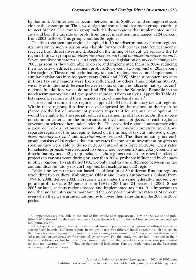
Notes: Number of regions in each group in parentheses.
Figure 2. Classification of Control and Treatment Groups Based on Corporate ProfitTax Regimes.
One may wonder whether nondiscriminatory and discriminatory tax cut treat-ment regions are geographically clustered, violating SUTVA. Figure 2 maps the ge-ographical locations of the different control and treatment groups listed in Table 1.It does not show any clear pattern that either nondiscriminatory or discriminatorytax cut regions are geographically clustered, though they do tend to be located inthe western part of Russia.
To systematically test the differences between control and treatment regionsin various dimensions during the pretreatment period before 2003, Table 2
Journal of Policy Analysis and Management DOI: 10.1002/pamPublished on behalf of the Association for Public Policy Analysis and Management

Corporate Tax Cuts and Foreign Direct Investment / 985
provides the difference of means tests between treatment (nondiscriminatory taxcut1/discriminatory tax cut1) and control (no tax cut) groups over a large numberof covariates, with covariate definitions discussed in detail in the following section.These t-tests apply a generous significance level (20 percent) and show systematicsimilarities and differences between treatment and control groups. It is useful tonote that treatment and control groups are statistically identical with respect tomany important covariates such as natural resources, labor cost, population, andgross regional product (GRP) growth. But panel 1 of Table 2 shows significant differ-ences between no tax cut and nondiscriminatory tax cut1 regions with respect to FDIbefore 2003, GRP per capita, public officials per capita, share of employees with highschool education, road density, criminality, urbanization, and control of corruption,and panel 2 shows significant differences between no tax cut and discriminatorytax cut1 regions with respect to trade, investment risk rating, spatial lag, privatiza-tion, share of employees with high school education, criminality, urbanization, budgetdeficit, and total domestic direct investment.
These significant differences between treatment and control groups should causeconcern if they point to potential endogeneity and systematic biases that determineboth tax policies and investments. In an influential theoretical study with someevidence on Russian regions, Cai and Treisman (2005) argue that, given capital mo-bility and asymmetric initial endowments (e.g., natural resources, human capital,etc.), governments in better endowed regions tend to invest more in infrastructure,adopt more business-friendly policies such as tax cuts, and thus attract more cap-ital. In contrast, governments in more poorly endowed regions often give up oncompeting for capital. For our analysis, the argument of Cai and Treisman (2005)implies that endowment conditions could drive both tax cuts and FDI flows, withbetter endowed regions more likely to cut taxes and attract more FDI.
The t-test results in Table 2 do not offer compelling evidence for this type of taxcut endogeneity. On the one hand, two patterns in the t-tests are contrary to the Caiand Treisman (2005) expectation. First, nondiscriminatory tax cuts occur in regionsthat are inferior to no tax cut regions with respect to FDI flows, GRP per capita,employees with high school education, crime rate, and urbanization during the pre-treatment period; discriminatory tax cuts occur in regions that are inferior withrespect to investment risk, privatization, employees with high school education,crime rate, urbanization, and budget deficit. Second, tax cut and no tax cut regionsare statistically identical with respect to natural resources, labor cost, population,and GRP growth. On the other hand, though, consistent with the Cai and Treisman(2005) expectation, during the pretreatment period, no tax cut regions are inferiorto nondiscriminatory tax cut1 regions over road density and control of corruptionand to discriminatory tax cut1 regions over trade and total domestic direct invest-ment. In sum, strong evidence is lacking for tax cut endogeneity, but the limitedevidence in favor of the Cai and Treisman (2005) arguments suggests the need tocontrol for those systematic differences when we estimate the effects of tax cuts onFDI.
Given the small number of regions in the nondiscriminatory tax cut1 group, Ap-pendix Table A2 further provides qualitative information on those regions to assurethat there is no clear selection bias.5 Overall, this is a very diverse group of re-gions in terms of economic performance, level of development, economic structure,natural resources, attractiveness to foreign investors, and regional politics. For ex-ample, Perm Krai, Rostov Oblast, and the Udmurt Republic were rich regions with
5 All appendices are available at the end of this article as it appears in JPAM online. Go to the pub-lisher’s Web site and use the search engine to locate the article at http://www3.interscience.wiley.com/cgi-bin/jhome/34787.
Journal of Policy Analysis and Management DOI: 10.1002/pamPublished on behalf of the Association for Public Policy Analysis and Management

986 / Corporate Tax Cuts and Foreign Direct Investment
Table 2. Balancing tests of difference in means for control variables between control andtreated regions.
Panel 1Mean (notax cuts)
Mean(nondiscriminatory
tax cut1)
P-value fordifference in
means
FDI 8.67 7.95 0.02*GRP per capita 7.27 7.07 0.01*Population 7.15 7.27 0.33Trade 6.11 5.84 0.21GRP growth 3.06 3.04 0.90Natural resources 42.29 39.57 0.46Public officials per capita 0.01 0.01 0.16*Rating of investment risk 39.81 40.94 0.75Spatial lag 35.55 37.59 0.42Privatization 51.08 39.29 0.38Length of governor’s stay 4.76 4.77 0.99Employees with high
school education19.58 18.09 0.01*
Nominal wage per capita 100.46 100.36 0.97Road density 4.07 4.47 0.01*Criminality 7.41 7.54 0.003*Urbanization 69.65 64.13 0.001*Budget deficit −21.88 −34.30 0.26Control of corruption 0.39 0.41 0.10*Total domestic direct
investment5.70 5.79 0.55
Rating of economic risk 41.67 40.20 0.70Rating of investment
climate7.56 7.56 0.84
Panel 2Mean (notax cuts)
Mean(discriminatory
tax cut1)
P-value fordifference in
means
FDI 8.67 8.37 0.22GRP per capita 7.27 7.31 0.49Population 7.15 7.17 0.71Trade 6.11 6.37 0.11*GRP growth 3.06 3.03 0.81Natural resources 42.29 44.08 0.43Public officials per capita 0.01 0.01 0.54Rating of investment risk 39.81 43.58 0.11*Spatial lag 35.55 42.93 0.001*Privatization 51.08 37.67 0.11*Length of governor’s stay 4.76 5.11 0.21Employees with high
school education19.58 17.76 0.00*
Nominal wage per capita 100.46 101.55 0.51Road density 4.07 4.21 0.27Criminality 7.41 7.51 0.01*Urbanization 69.65 67.56 0.1*Budget deficit −21.88 −34.58 0.19*Control of corruption 0.39 0.40 0.36Total domestic direct
investment5.70 5.90 0.06*
Journal of Policy Analysis and Management DOI: 10.1002/pamPublished on behalf of the Association for Public Policy Analysis and Management

Corporate Tax Cuts and Foreign Direct Investment / 987
Table 2. Continued.
Panel 2Mean (notax cuts)
Mean(nondiscriminatory
tax cut1)
P-value fordifference in
means
Rating of economic risk 41.67 40.21 0.53Rating of investment
climate7.56 7.49 0.83
Notes:Tests assume control and treatment groups have unequal variances.Asterisk indicates that the difference in means between control and treatment groups is significantlydifferent from zero at the 20 percent significance level for the two-tailed test.
high per capita income and low unemployment, though the northern districts ofRostov Oblast were less wealthy. In contrast, Amur Oblast, Bryansk Oblast, andthe Chuvash Republic were poor regions with low per capita income and highunemployment. Some regions, like Amur Oblast, Rostov Oblast, and the UdmurtRepublic, had natural resources, but others did not. From the political perspec-tive, the governors in nondiscriminatory tax cut1 regions were also quite diverse.Some of these governors had stronger connections with the business communityor international organizations, for example, Yuri Trutnev of Perm Krai and Niko-lai Fedorov of the Chuvash Republic, while others seemed to have more autarkicpolicies, for example, Vladimir Chub of Rostov Oblast, or stronger ties with localcrime groups, for example, Nilolai Denin of Bryansk Oblast and Alexander Volkovof the Udmurt Republic, or corruption schemes, for example, Leonid Korotkov ofAmur Oblast. In sum, nondiscriminatory tax cut1 regions did not appear to haveany particular set of unifying attributes that could bias our analysis in a certaindirection.
PARAMETRIC DID ESTIMATION OF AVERAGE TREATMENT EFFECT
In comparative studies, researchers compare the units exposed to treatment with oneor more unexposed units (Abadie, Diamond, & Hainmueller, 2010). In estimatingthe effects of tax cuts on FDI using observational data, we do not observe the levelof FDI for the same unit in the absence of tax cut, making it difficult to consider theestimated effect to be causal. Ideally, to overcome this problem, we would conducta field experiment in which tax cuts were randomly assigned among 82 Russianregions. Given random assignment, we could simply compare regions that cut taxeswith those that did not. The difference in the average level of FDI between treatmentand control groups would constitute the effect of a tax cut. The rationale is thatrandom assignment produces a reliable policy counterfactual because it ensuresboth groups are comparable with respect to (un)observed confounders. Of course,in reality, tax cuts were never completely randomly assigned. In the absence ofcompletely randomized assignment, we have to rely on quasi-experimental methodsto approximate randomization when using observational data (Angrist & Pischke,2008; Holland, 1986; Rubin, 1974, 1977). This is why, in the previous section, wetook great care to create roughly similar control and treatment groups.
The DID estimation allows us to approximate randomization by design. Followingthe regression DID framework discussed in Angrist and Pischke (2008), hypotheticalestimation may take the following form in the context of FDI and tax cuts betweenone treatment and one control region:
F DIit = β1 + β2Treati + β3Cutt + β4 (Treati × Cutt) + εit (1)
Journal of Policy Analysis and Management DOI: 10.1002/pamPublished on behalf of the Association for Public Policy Analysis and Management

988 / Corporate Tax Cuts and Foreign Direct Investment
where F DIit denotes observed FDI inflows in region i at period t, εit denotes inde-pendent and identically distributed random error, Treati indicates a dummy for thetreated region that cuts tax at some point relative to the control region, β2 denotesthe time-invariant regional difference between treated and control regions in theabsence of a tax cut (fixed effect), Cutt denotes a time dummy that equals 1 after atax cut kicks in, β3 denotes the tax cut year-specific effect common to both regions,and (Treati × Cutt) denotes the interaction between the treated region and the taxcut year dummy. In this setup, β4 denotes the DID effect of interest, that is, theaverage treatment effect of tax cuts on FDI.
The setup in equation (1), when applied to our analysis, requires several modifi-cations. First, even within each group (treatment or control), we have many regionsthat have unobserved heterogeneity for which we need to account. Hence, we in-clude a fixed effect dummy for each region ηi instead of β2Treati .6 Second, insteadof one tax cut year, we have multiple pretax-cut and tax-cut years that each mighthave a year-specific effect common to all regions (e.g., 2002 experienced a wholecountrywide tax cut even though it preceded the regional tax cut years). Hence,we include a year fixed effect dummy for each year, θt, instead of β3Cutt.7 Third,we have two different types of tax cuts enacted by treated regions in 2003 andimplemented in 2004. Hence, we have to estimate the effects of two types of taxcut treatments separately. Specifically, Nondiscriminatory × Cut1 is a dummy thatscores 1 for nondiscriminatory tax cut1 regions since 2003 and zero before 2003.Discriminatory × Cut1 is a dummy that scores 1 for discriminatory tax cut1 regionssince 2003 and 0 otherwise. Their coefficients represent the DID effects of respectivetax cuts on FDI. Finally, we have to control for observed possible confounding co-variates, particularly those over which treated and control regions are not balancedin Table 2. Thus, our DID regression model is specified as follows:
F DIit = β1 + β2 Nondiscriminatory × Cut1i,t−1 + β3 Discriminatory × Cut1i,t−1
+β4 F DIi,t−1 + β j Xi,t−1 + ηi + θt + εit (2)
FDI is known to have inertia since all MNEs consider reinvestment in orderto stay in the host. We model such temporal dependence by including the laggeddependent variable, F DIi,t−1, on the right-hand side. Other control variables, repre-sented by Xi,t−1,include GRP per capita, trade, investment risk, number of publicofficials per capita, human capital, privatization, urbanization, crime rate, budgetdeficit, transportation infrastructure, spatial correlation, control of corruption, andtotal domestic direct investment. All right-hand side variables are those over whichtreated and control groups are imbalanced. Time-varying covariates are lagged oneyear to avoid the posttreatment bias. Data for all variables come from Rosstat unlessindicated otherwise.
GRP per capita, measured in constant 2000 U.S. dollars and log transformed, re-flects the level of economic development in a region for a given year. The variabletrade, measured as the logged sum of import and export of a region, controls for theeffect of trade on FDI, which could be positive (e.g., intrafirm trade) or negative (e.g.,tariff jumping investment) (Neary, 2009). The number of public officials per capitais a crude proxy for the lack of bureaucratic quality in a region. Inflated bureau-cracy is often associated with greater administrative burdens, discouraging foreigninvestors. The share of employees with high school education in total employment
6 The Hausman test shows that region fixed effects are preferred to region random effects.7 Wald test confirms that year fixed effects are necessary.
Journal of Policy Analysis and Management DOI: 10.1002/pamPublished on behalf of the Association for Public Policy Analysis and Management

Corporate Tax Cuts and Foreign Direct Investment / 989
controls for the quality of labor, which may help attract investment (Broadman &Recanatini, 2001). We also control for logged road density and percentage of urbanpopulation because transport infrastructure and urbanization reduce transporta-tion costs for foreign investors and can facilitate their market expansion (Iwasaki& Suganuma, 2005; Kayam, Hisarciklilar, & Yabrukov, 2007; Ledyaeva, 2007). Inaddition, we also control for criminality (number of crimes per 100,000 persons) be-cause social conflict and criminal violence are shown to discourage foreign investors(Broadman & Recanatini, 2001).
The SUTVA assumption requires no interference between units, but FDI flowstend to be associated with spatial correlation (Bradshaw, 1997, 2002; Ledyaeva,2007). We examine the spatial correlation of FDI using Moran’s I statistics for threedifferent years (1995, 2002, 2008). The results indicate the absence of spatial correla-tion in FDI in 1995, but significant negative correlation among regions during 2002and 2008. Hence we include in the model a variable spatial lag of FDI. Specifically,we multiply the lagged dependent variable by a connectivity matrix that capturescontiguity among the Russian regions in our sample. The connectivity matrix hasones for those regions that share the border and zeros for those regions that do not.8
Foreign investors often have to consider the impact of investment risks derivedfrom operating in a foreign country. The investment risk rating, compiled by theRussian rating agency Expert, ranges from 1 to 82, with 1 indicating the lowest risk.The variable takes into account political, social, criminal, ecological, financial, andadministrative risks investors might face in a region. It is widely used in previousstudies (see, e.g., Broadman & Recanatini, 2001) and should have a negative sign.
Corruption is a notorious problem for businesses in Russia. Since it might affectboth tax policy and FDI, it should be controlled for in our analysis. However, deter-mining the true level of corruption is always problematic. We use several pieces ofinformation to create an indicator for the underlying level of severity of corruptionat the regional level. First, we collected data on four different regional indicators,including the following:
1. Regional Democracy Index by the Independent Institute for Social Policy,9
based on expert evaluations of the regional democracy level in 1991 to 2004 andrepresenting the sum of scores in 10 categories (transparency, fair elections,political pluralism, independent media, economic liberalization, civil societystrength, system of checks and balances, regional elite strength, corruption,and local self-governance);
2. Electoral Democracy Index by the Independent Institute for Social Policy,based on instrumental assessments of fairness and transparency of the elec-tions held in the 1991 to 2002 electoral cycles and representing the averagescore of 11 indicators (voter turnout in federal elections, voter turnout in re-gional elections, competitiveness in federal elections, competitiveness in elec-tions for regional legislature, competitiveness in elections for regional gov-ernor, number of votes Against All [AA] in elections for regional governor,number of AA votes in federal elections, number of AA votes in elections forregional legislature, change of incumbent after elections, electoral frauds inregional elections, and electoral frauds in federal elections);
8 We use the lagged dependent variable in the spatial lag (rather than modeling a simultaneous effect ofFDI) to avoid endogeneity in estimating such a model (Beck, Gleditsch, & Beardsley, 2006).9 Full description of sources and methodology for Regional Democracy Index, Electoral DemocracyIndex, and Index of Corruption is available from the Social Atlas of Russian Regions by the IndependentInstitute for Social Policy (in Russian only) at http://atlas.socpol.ru/indexes/index_democr.shtml.
Journal of Policy Analysis and Management DOI: 10.1002/pamPublished on behalf of the Association for Public Policy Analysis and Management

990 / Corporate Tax Cuts and Foreign Direct Investment
3. Index of Corruption by the Independent Institute for Social Policy, based onexpert evaluations both of the degree of interconnection between political andbusiness elites and of corruption scandals for particular years; and
4. Bribery Index by the OPORA RUSSIA Foundation and the Russian Public Opin-ion Research Center (VCIOM), based on the results of a joint survey “Conditionsand factors of the small business development in the regions of Russia”10 heldin 2004 to 2005, when business executives were asked “How wide-spread is thepractice of ‘solving problems’ with officials through bribing them?,” with theiranswers then transformed into a weighted score.
We rescale all four indicators so that they are bounded between 0 and 1 (withhigher values indicating less corruption), and then combine them into one variablecontrol of corruption. Second, as the four indicators are measured at various timepoints, the combined index has many missing values. Therefore, we impute themissing values using linear interpolation as a function of GRP per capita, whichis highly correlated with each component of our indicator of corruption. We dou-ble check that values of the final index correspond to the qualitative evidence oncorruption in various Russian regions. For instance, the Republic of Dagestan isshown as one of the most corrupt regions in our sample, whereas Tambov Oblastand Novosibirsk Oblast are shown to be the least corrupt. The variable control ofcorruption is negatively correlated with the severity of corruption and should havea positive sign.
Both regional budget constraints and independence from federal transfers mayaffect the regions’ willingness to implement tax cuts. To capture this possibility, weinclude logged regional deficit, measured in constant 2000 U.S. dollars and computedas [Regional budget revenue − (Budget transfers from federal budget + Regionalbudget expenses)]. The variable is expected to have a negative sign.
The effect of tax cuts could be spurious if tax cuts are part of an across-the-boardliberalization reform. The region fixed effects help to account for any heterogene-ity among regions, and the year fixed effects control for system-wide shocks andreforms implemented by the federal government (e.g., trade liberalization). Mean-while, the studies of other types of reforms implemented in Russia around 2003allow us to rule out the possibility that other reforms could act as confoundingfactors. To the best of our knowledge, there is no evidence of a reform of the la-bor market regulations between 2002 and 2006 (Denisova, Eller, & Zhuravskaya,2007; Gimpelson & Kapeliushnikov, 2011), changes in industrial regulations be-tween 1999 and 2008 (Vinhas de Souza, 2008b), or of changes in the reduction ofinformal barriers (Cheloukhine & King, 2007).
Still, tests in Table 2 suggest systematic differences in terms of privatization anddomestic investment between discriminatory tax cut1 and no tax cut regions, butnot between nondiscriminatory tax cut1 and no tax cut regions. Since privatizationwas a salient policy reform in Russia and the volume of domestic investment shouldalso correlate with the outcome of relevant reforms, we control for these two vari-ables in our model. The variable privatization measures the number of companiesprivatized in a region in a given year. Although privatization reforms were decidedby the federal government, we control for it to isolate the effects of other correlatedinstitutional reforms. Domestic direct investment measures total investment of do-mestic enterprises in fixed assets, measured in constant 2000 U.S. dollars and logtransformed.
10 The complete survey report is available from the Russian Public Opinion Research Center (VCIOM)database (in Russian only) at http://wciom.ru/russian-support/.
Journal of Policy Analysis and Management DOI: 10.1002/pamPublished on behalf of the Association for Public Policy Analysis and Management

Corporate Tax Cuts and Foreign Direct Investment / 991
In addition, we also control for economic risk rating and investment climate ratingas additional robustness check variables to capture possible effects of broad liberal-ization reforms in Russia. Economic risk rating ranges from 1 to 82, with 1 indicat-ing the lowest risk. The variable is based on assessments of economic risk relatedto proposed economic reforms, inflation, retail trade, and consumption at the re-gional level. The investment climate rating reflects the overall quality of institutionalpolicies, specifically created by regional governments to promote investment (e.g.,stability and completeness of the regional investment legislation, equal treatment ofboth domestic and foreign investors, support for small enterprises investment, etc.).Both variables are created by the Russian rating agency Expert.
Previous studies of FDI also often control for the following variables: population,real economic growth, natural resources potential, political stability, and labor costs.While Table 2 shows that treatment and control groups are balanced over thesefactors, we control for their effects in a robustness check to ensure the validity of ourresults. The logged variable population accounts for regional market size, often animportant driver in attracting FDI, and it also acts as a proxy for regional labor force(Ahrend, 2000; Ledyaeva, 2007). The variable real economic growth (GRP Growth)is another traditional measure of regional economic development. Next, FDI oftendepends on the presence of natural resources, which turned out to be significantin some previous studies (Asiedu & Lien, 2011; Kayam, Hisarciklilar, & Yabrukov,2007). We control for regional rating of natural resources potential, compiled by theRussian ratings agency Expert. The governor’s tenure in office is a proxy for politicalstability in a region. Longer governor tenure is associated with more stable andpredictable policies, reducing uncertainty for investors. Following Broadman andRecanatini (2001), we control for labor cost with real growth of nominal wages.11
Table 3 presents descriptive statistics on all variables of interest in the estimationsample and their sources, and Appendix Table A3 shows the correlation among allcovariates.12
Since we have both the lagged dependent variable and region fixed effects on theright-hand side, ordinary least squares estimates are biased (Nickell, 1981). Hencewe use the Arellano–Bover/Blundell–Bond system GMM estimator. It employs themoment conditions of lagged levels as instruments for the differenced equation to-gether with the moment conditions of lagged differences as instruments for the levelequation. The generalized method of moments (GMM) estimator helps to identifythe effects of time-invariant variables, provides a larger set of moment conditionsboth to overcome some weak instruments biases of first differenced estimators andto reduce the finite sample bias in panels with short T and persistent regressors.This further enables us to address the endogeneity of multiple variables with ap-propriate instruments (see, e.g., Arellano & Bover, 1995; Baltagi, 2005; Blundell &
11 In an unreported robustness check, we also include a dummy variable for whether or not a regionhas a special economic zone (SEZ). The SEZs were created in some regions in the forms of industrialareas, tourism zones, and innovation parks. Businesses in a SEZ received tax holidays for the first 10 to15 years of their activity and paid zero import tariffs. However, most SEZs were established in 2006 to2007 and became fully functional around 2009 to 2010, making them less relevant to our analysis. In ourestimation, the effect of SEZ is not statistically significant, and their inclusion does not affect the effectsof tax cut variables.12 All appendices are available at the end of this article as it appears in JPAM online. Go to the pub-lisher’s Web site and use the search engine to locate the article at http://www3.interscience.wiley.com/cgi-bin/jhome/34787.
Journal of Policy Analysis and Management DOI: 10.1002/pamPublished on behalf of the Association for Public Policy Analysis and Management

992 / Corporate Tax Cuts and Foreign Direct Investment
Table 3. Descriptive statistics.
Variable Obs. Mean Std. dev. Min. Max. Source
FDI (log) 567 9.41 2.41 0.69 16.38 Rosstat (2012)Nondiscriminatory tax
cut regions567 0.06 0.24 0 1 Authors’
calculationsDiscriminatory tax cut
regions567 0.24 0.43 0 1 Authors’
calculationsGRP per capita 567 7.55 0.68 6.08 9.94 Rosstat (2012)GRP growth 567 3.11 0.94 −4.46 4.77 Rosstat (2012)Population 567 7.34 0.71 5.11 9.26 Rosstat (2012)Trade 567 6.80 1.45 2.34 12.08 Rosstat (2012)Natural resources 567 42.07 24.03 1 82 Rating agency
Expert (2012)Rating of investment
risk567 40.42 23.31 1 82 Rating agency
Expert (2012)Length of governor’s
stay567 6.56 4.09 1 18 Authors’
calculationsPublic officials per
capita567 0.01 0.003 0.004 0.034 Rosstat (2012)
Spatial lag 567 50.26 18.16 14.8 107 Authors’calculations
Nominal wage percapita
567 108 13.16 68.5 135.9 Rosstat (2012)
Employees withsecondary education
567 20.67 4.71 11.7 48.5 Rosstat (2012)
Privatization 567 18.59 35.65 0 351 Rosstat (2012)Road density 567 4.36 1.21 1.36 6.5 Rosstat (2012)Criminality 567 7.65 0.31 6.69 8.51 Rosstat (2012)Urbanization 567 71.82 10.12 52.4 100 Rosstat (2012)Budget deficit 567 −97.65 378.58 −1586.72 7476.23 Rosstat (2012)Control of corruption 567 0.41 0.07 0.22 0.58 Authors’
calculationsTotal domestic direct
investment567 6.55 1.17 3.73 10.34 Rosstat (2012)
Rating of economicrisk
567 42.12 23.75 1 82 Rating agencyExpert (2012)
Rating of investmentclimate
567 8.07 2.70 1 13 Rating agencyExpert (2012)
Bond, 2000; Roodman, 2009a).13 We also estimate robust standard errors to correctfor heteroskedasticity.14
RESULTS OF DID ESTIMATION
Table 4 shows the DID estimation results. For the system GMM estimator to be valid,several assumptions and diagnostic tests are important. First, the error term shouldbe free from serial correlation for the instruments to be valid. With first differencing
13 We treat lagged dependent variable, per capita GRP, share of public officials, and road density as en-dogenous and all other lagged covariates as exogenous. When we change the variables that are treated asendogenous, the results remain robust. Variance inflation factor statistics for the tax cut variables showno concern for multicollinearity.14 Breusch–Pagan test shows that we need to correct for heteroskedastacity.
Journal of Policy Analysis and Management DOI: 10.1002/pamPublished on behalf of the Association for Public Policy Analysis and Management

Corporate Tax Cuts and Foreign Direct Investment / 993
Table 4. Difference in Differences Estimation Based on System GMM Model.
(1) (2) (3) (4) (5)Variables ln(FDI) ln(FDI) ln(FDI) ln(FDI) ln(FDI)
Tax Level −0.071(0.171)
Non-discriminatory tax cut 1.585* 1.501* 1.207**
(0.815) (0.781) (0.593)Discriminatory tax cut 0.274 0.218 −0.036
(0.516) (0.515) (0.607)Lagged FDI 0.296*** 0.288*** 0.286*** 0.369***
(0.090) (0.089) (0.077) (0.109)Lagged FDI (2-year) 0.205** 0.134**
(0.104) (0.063)GRP per capita −0.151 −0.127 −0.752
(0.538) (0.549) (0.615)Trade −0.875** −0.876** −0.885***
(0.348) (0.343) (0.335)Public Officials per capita 33.669 66.682 122.153
(90.397) (103.784) (228.905)Rating of Investment Risk −0.013** −0.013** −0.019***
(0.006) (0.005) (0.006)Spatial Lag −0.079*** −0.078*** −0.082***
(0.021) (0.022) (0.022)Privatization 0.002 0.002 0.002
(0.004) (0.004) (0.004)Employed with Secondary Education 0.022 0.020 0.017
(0.027) (0.026) (0.027)Road Density 2.346 2.310 0.297
(2.480) (2.456) (0.658)Criminality 1.106 1.249 1.098
(0.851) (0.861) (0.866)Urbanization −0.151 −0.131 −0.119
(0.159) (0.152) (0.152)Budget Deficit −0.000* −0.000* −0.000***
(0.000) (0.000) (0.000)Control of Corruption 5.470** 5.508** 6.435**
(2.724) (2.672) (3.011)Total Domestic Direct Investment 0.161 0.199 0.407
(0.353) (0.362) (0.395)Population 3.098
(7.060)GRP Growth 0.110
(0.080)Rating of Natural Resources −0.006
(0.043)Length of Governor’s Stay in Power −0.009
(0.028)Real Growth of Wages −0.000
(0.014)Rating of Economic Risk 0.009*
(0.005)Rating of Investment Climate 0.076
(0.056)Arellano-Bond test for AR(1) 0.00*** 0.00*** 0.00*** 0.00*** 0.00***
Arellano-Bond test for AR(2) 0.143 0.152 0.183 0.291 0.891Sargan test – χ2 40.68 39.12 31.45 32.18 15.09Sargan-Hansen test – χ2 36.58 35.71 21.72 11.43 16.70*
Region FE yes yes yes yes YesYear FE yes yes yes yes YesObservations 567 567 565 338 500Number of instruments 58 59 55 22 23Number of id 59 59 59 36 53
Notes: Robust standard errors in parenthesesCoefficients and standard errors of the main explanatory variables are in bold.***p < 0.01, **p < 0.05, *p < 0.1 for two-tailed tests
Journal of Policy Analysis and Management DOI: 10.1002/pamPublished on behalf of the Association for Public Policy Analysis and Management
994 / Corporate Tax Cuts and Foreign Direct Investment
in the system GMM, the differenced errors should be serially correlated at order 1,but not at any higher order. Hence, serial correlation tests in first differenced resid-uals should be significant for AR(1), but not for AR(2). Second, the instrumentsshould be exogenous. The Sargan–Hansen overidentification restriction tests allowone to verify the joint null hypothesis that the instruments are valid and uncorre-lated with the error term and that the excluded instruments are correctly excluded.Finally, the number of instruments should be smaller than either the number ofobservations or the number of panels, which helps to prevent overfitting the en-dogenous variables and artificially reducing standard error estimates (Roodman,2009b). Results for all diagnostics in Table 4 are reassuring.15
Table 4 reports the results for five models. Model 1 follows the literature by includ-ing a continuous variable for the corporate profit tax rate and ignoring tax regimedifferences among regions. It measures the lowest possible corporate profit tax ratefor each region, which equals the flat rate for no tax cut regions, the reduced rateon direct investment profit for nondiscriminatory tax cut1 regions, and the reducedrate on select important investment projects for discriminatory tax cut1 regions. Asnoted, this continuous measure masquerades the fact that different regions imple-mented distinct tax policies. Its estimated effect has the expected negative sign, butis statistically insignificant. Mixing different tax policies into one seemingly coher-ent continuous measure of tax rate may have distorted the estimated effect of taxcuts.
Model 2 is our primary model, based on our carefully crafted sample designthat compares no tax cut regions with nondiscriminatory tax cut1/discriminatorytax cut1 regions, respectively, and including only the imbalanced covariates. Thesethree groups consist of 69 regions, which drops down to 59 due to missing valuesof the variables. Model 2 includes the two tax cut dichotomous variables, the laggeddependent variable, and all the covariates on which treatment and control groupsare imbalanced as shown in Table 2. Only a few control variables have statisticallysignificant effects in Models 1 and 2, a pattern in line with previous studies onFDI in Russia (Strasky & Pashinova, 2012). It also is because we have extensivecontrols in the models (lagged FDI, region, and year fixed effects). Furthermore, theeffects of significant variables are consistent with our expectations. In sum, FDI inRussian regions exhibits strong path dependence and negative spatial correlation,is negatively correlated with regional trade and budget deficit, and flows to areaswith lower investment risk and corruption.
In Model 2, the coefficients of both nondiscriminatory tax cut and discriminatorytax cut are positive, but only the former is statistically significant at the conventionallevel. Thus, Model 2 suggests that tax cuts on direct investment profit increase FDIinflows, but tax cuts on profits from select important investment projects do not.
How large is the average treatment effect of the nondiscriminatory tax cut? If werely on the estimate in Model 2 (1.59), the size of the treatment effect on FDI betweennondiscriminatory tax cut and no tax cut regions is [
(e1.59 − −1
) × 100]. Thus theannualized percentage change in FDI for each year during the 2003 to 2008 periodshould be
[(e1.59 − −1
) × 100]/6. On average, relative to the no tax cut regions, tax
cuts on direct investment profit increase FDI flows into nondiscriminatory tax cut1regions by slightly over 65 percent per year during the 2003 to 2008 period. Thisestimate demonstrates the substantial effect of one type of tax cut reforms.16
15 The only possible exception is Model 5, for which the results of the exogeneity test are less clear. Model5 passes the Sargan test, but fails the Hansen test.16 Note that this treatment effect estimate is not directly comparable with the semielasticity (or tax rateelasticity) estimates in the literature, which measures the percentage change in FDI due to a 1 percentage
Journal of Policy Analysis and Management DOI: 10.1002/pamPublished on behalf of the Association for Public Policy Analysis and Management

Corporate Tax Cuts and Foreign Direct Investment / 995
Model 3 in Table 4 reports the results of one robustness test that includes ad-ditional covariates. Even though treatment and control groups are balanced overthese variables, we estimate the model to check whether our findings are sensitiveto their inclusion or not. Results for tax cut variables remain robust as in Model 2,which is reassuring. We should also note that as expected, the additional covariatescollectively have very little explanatory power.
One possible issue with Model 2 is that several time-varying covariates couldpotentially be endogenous, producing posttreatment bias. Even though their inclu-sion is justified by the lack of balancing between treatment (nondiscriminatory taxcut1/discriminatory tax cut1) and control (no tax cut) groups, they could poten-tially be affected by tax cut and FDI. The most recent balancing technique, alsoknown as entropy balancing, could help to address this problem. This new methodcreates weights based on covariates along which treatment and control groups arevery different (imbalanced). With these weights, treatment and control groups aremade most similar with respect to those imbalanced covariates. One can then esti-mate a DID model using the simplest specification: controlling for lagged FDI andcountry and year fixed effects for path dependence and unobservables, but withoutany other independent variables since balancing has made treatment and controlregions identical for those covariates.
Concretely, we implement the following procedures. First, in the pretreatmentperiod we balance the covariates with significantly different means between nondis-criminatory tax cut1 and no tax cut regions using the Stata 12 command ebalance.We do the same for the unbalanced covariates for discriminatory tax cut1 and no taxcut regions.17 Appendix Table A3 shows that after balancing, the means of all thesecontrol variables are exactly the same between treatment and control regions.18 Sec-ond, we use the weights obtained by entropy balancing in the pretreatment periodalso in the posttreatment period, that is, for the years 2003 to 2008 we use the 2002weights. As noted, we do so to avoid any posttreatment bias, that is, our treatmentsmight affect some control variables in the posttreatment period. Third, we rerun theGMM estimation with the simplest specification noted above and using the weightsfrom ebalance. Since we have two treatments, that is, nondiscriminatory tax cut1and discriminatory tax cut1, we have to run two different estimations. This is be-cause the two treatment groups are imbalanced with the control group with respectto different covariates, causing the weights to differ for the two samples. Models 4and 5 in Table 4 show the results for two comparisons: nondiscriminatory tax cut1vs. no tax cut and discriminatory tax cut1 vs. no tax cut, respectively. The resultsare consistent with the findings in Models 2 and 3, with slightly stronger statisticalsignificance, but slightly weaker substantive effect for nondiscriminatory tax cut1.
Therefore, based on the results in Table 4, we conclude that tax cuts on directinvestment profit cause significantly more FDI inflows than no tax cuts, but taxcuts on selective important investment projects do not. Not all tax cuts significantlyincrease FDI inflows. These findings are robust when we add more control variablesand use alternative estimation strategies.
To further diagnose the validity of our findings in Table 4, we implement threeplacebo tests. In Table 5, we first rerun our baseline model replacing the dependentvariable FDI with two variables that should be orthogonal to tax cuts: number
point change in the tax rate. In a meta-analysis on taxation and FDI, De Mooij and Ederveen (2003) showthat of the 371 semielasticity estimates from 25 taxation–FDI studies, their mean semielasticity estimateis −4.7, their maximum–minimum ranges between −84.5 to 17.8.17 We specify the order of moment constraints (i.e., targets) equal to 2. Results, available upon request,are similar if we use targets equal to one or three.
Journal of Policy Analysis and Management DOI: 10.1002/pamPublished on behalf of the Association for Public Policy Analysis and Management

996 / Corporate Tax Cuts and Foreign Direct Investment
Table 5. Placebo Tests.
(6) (7) (8)Variables Female alcoholism Female suicide ln(FDI)
Non-discriminatory tax cut −2.284 −1.274(5.939) (0.940)
Discriminatory tax cut 1.098 0.290(4.301) (0.665)
Non-discriminatory tax cut (lead) −0.588(0.512)
Discriminatory tax cut (lead) −0.131(0.374)
Lagged Female Alcoholism 0.527***
(0.176)Lagged Female Suicide 0.078
(0.068)Lagged FDI 0.273***
(0.102)GRP per capita 20.991* 1.258 0.045
(12.622) (1.048) (0.579)Trade −2.282 0.978 −0.858**
(3.273) (0.640) (0.364)Public Officials per capita −2,235.967 556.301 56.872
(1,799.558) (638.316) (112.856)Rating of Investment Risk 0.024 0.010 −0.013**
(0.054) (0.008) (0.005)Spatial Lag −0.379* −0.021 −0.076***
(0.223) (0.031) (0.022)Privatization −0.010 0.004* 0.002
(0.024) (0.003) (0.004)Employees with Secondary education 0.063 −0.021 0.020
(0.255) (0.077) (0.027)Road Density −23.540 −7.005 1.767
(25.764) (6.044) (2.531)Criminality −5.126 −1.761 1.054
(11.510) (1.702) (0.820)Urbanization −1.842 0.155 −0.110
(1.501) (0.182) (0.151)Budget Deficit −0.001 0.000 −0.000
(0.001) (0.000) (0.000)Control of Corruption 58.460* 2.899 6.976**
(33.737) (3.833) (2.930)Total Domestic Direct Investment 3.471 −0.028 0.142
(5.279) (1.059) (0.371)Arellano-Bond test for AR(1) 0.00*** 0.00*** 0.000Arellano-Bond test for AR(2) 0.872 0.622 0.155Sargan test – χ2 115.52 25.84*** 32.95*
Sargan-Hansen test – χ2 24.41 25.841 22.37Region FE yes yes yesYear FE yes yes yesObservations 457 649 567Number of instruments 44 47 49Number of id 66 66 59
Notes: Robust standard errors in parentheses.Coefficients and standard errors of the main explanatory variables are in bold.***p < 0.01, ** p < 0.05, *p < 0.1 for two tailed tests.
Journal of Policy Analysis and Management DOI: 10.1002/pamPublished on behalf of the Association for Public Policy Analysis and Management

Corporate Tax Cuts and Foreign Direct Investment / 997
of deaths by alcoholic intoxication in female population and number of femalesuicides. We expect a tax cut to have no effect on those variables. If it does, itwould imply that nondiscriminatory tax cut1 and discriminatory tax cut1 regionsdiffer substantially from no tax cut regions in some aspects we fail to consider,thus invalidating our identification strategy. Therefore, it is reassuring that bothnondiscriminatory tax cut1 and discriminatory tax cut1 region treatments are neverstatistically significant at the conventional level in Table 5.
In another placebo test, we replace our two treatments in the full model with twodummies that score 1 for nondiscriminatory tax cut1 and discriminatory tax cut1regions, respectively, in the pretreatment years from 2000 to 2002 and 0 otherwise.The expectation is that if our DID analysis is valid, the leading nondiscriminatorytax cut1 and discriminatory tax cut1 variables should have no effect on FDI. Asexpected, neither pretreatment dummy, commonly referred to as leads in the DIDliterature, has any statistically significant effect.
NONPARAMETRIC SCM FOR LOCAL TREATMENT EFFECTS
Even though we separate different regions into various relatively homogeneoustax regime groups to estimate the average treatment effect in parametric analysis,different regions under the same tax policy regime (say, nondiscriminatory tax cut1)could still be rather different. In this case, the average treatment effect does not tellus how effective a tax cut in each individual region is. Hence, for thorough policyevaluation, it is useful to identify the local policy treatment effect specific to eachregion. This is possible if we could construct the most similar counterfactual to eachregion for comparison. In addition, DID estimation is “based on the presumptionof time-invariant (or group-invariant) omitted variables” (Angrist & Pischke, 2008,p. 243), as reflected in our region fixed effects. For many cause-effect questions,including ours, the idea that omitted variables are time-invariant may not alwaysbe plausible.
To address these issues, we complement the parametric DID estimation usingthe SCM—a nonparametric estimation technique, which allows us to build a cred-ible counterfactual to identify the local treatment effect (Abadie, 2005; Abadie &Gardeazabal, 2003). The SCM was pioneered by Abadie and Gardeazabal (2003) ina study of terrorism in the Basque Country and further developed by Abadie, Dia-mond, and Hainmueller (2010). The idea behind SCM is simple: a combination ofcomparison units as a synthetic control often resembles the attributes of the treatedunit more closely than any single control unit alone. In other words, the SCM ap-proach allows us to build a credible counterfactual to identify the local treatmenteffect of tax cut on FDI for a region over a certain period.
How does SCM work for our analysis? We test whether a tax cut adopted bya region i in 2003 and implemented in 2004 leads to more FDI inflow into theregion during the 2003 to 2008 period when it is compared with a syntheticallyconstructed control unit that resembles the treated region as closely as possible forthe same period. Because comparison units are meant to approximate the coun-terfactual without the treatment, SCM restricts the donor pool for constructing thecounterfactual to those regions with outcomes that are thought to be driven bythe same structural process as the treated region, but that are not subject to thesame tax cut regimen during the period of study (Abadie, Diamond, & Hainmueller,
18 All appendices are available at the end of this article as it appears in JPAM online. Go to the pub-lisher’s Web site and use the search engine to locate the article at http://www3.interscience.wiley.com/cgi-bin/jhome/34787.
Journal of Policy Analysis and Management DOI: 10.1002/pamPublished on behalf of the Association for Public Policy Analysis and Management

998 / Corporate Tax Cuts and Foreign Direct Investment
2012). The comparison regions, which constitute the synthetic controls group, areselected using an algorithm based on their similarity to the treated region, i, beforethe treatment, both with respect to confounding factors and the past level of FDI. Inother words, “the synthetic control algorithm estimates the missing counterfactualas a weighted average of the outcomes of potential controls” (Billmeier & Nannicini,2013, p. 987).
Key elements of SCM are the weights of the synthetic control units. Specifically,the synthetic controls algorithm estimates the weights in a nonparametric way sothat the distance (or pseudodistance) in terms of the vector of pretreatment covari-ates between the treated region and the potential synthetic control is minimized.19
Let us take Amur Oblast, a treated nondiscriminatory tax cut1 region, as an example.The synthetic controls algorithm detects the closest regions to Amur Oblast accord-ing to a large number of characteristics captured by the control variables among allno-tax-cut regions. We can then compute the difference in terms of the change inFDI from pretreatment to posttreatment periods between Amur Oblast and the syn-thetic control unit as the local treatment effect specific to Amur Oblast. We repeatthis procedure for all treated regions (both nondiscriminatory and discriminatorytax cut1 regions).
More specifically, to build the synthetic controls group, we use all regions in theno-tax-cut group to increase the power of our tests. We approximate all the unbal-anced control variables, which we described in the parametric estimation, in thepretreatment period. We also include the lagged dependent variable in the pretreat-ment period to rule out anticipatory effects. All predictor variables are averagedover the entire pretreatment period (1995 to 2002).20 We use the average value ofthe outcome variable over the pre- and posttreatment periods because FDI flows areknown to be volatile, with extremely large values in some years, but very small valuesin others, and we are interested in the average effect over the years. Averaging FDIflows over the pre- and posttreatment periods helps to remove such idiosyncraticnoise, producing more credible local treatment effect estimates.
The SCM approach has several different strengths when compared with para-metric estimation (Abadie, Diamond, & Hainmueller, 2010; Billmeier & Nannicini,2013). As a main advantage, SCM makes the comparison more directly relevant toeach region than in parametric estimation since the control group can be restrictedto those regions most similar to the treated unit with respect to most relevant co-variates. Therefore, SCM identifies the local treatment effect for each treated regionrelative to the most similar counterfactual one could potentially construct. It offersan in-depth understanding of the effect of a policy change for each treated unitrelative to its most similar counterfactual. Another strength of SCM is its trans-parency because the comparison regions that end up in the counterfactual, as wellas their weights, can be easily identified. Appendix Tables A5 and A6 report theweights assigned to each donor region that contributes to counterfactual constructsfor nondiscriminatory tax cut1 and discriminatory tax cut1 regions, respectively.21
Finally, SCM allows the use of both qualitative and quantitative information, for-malizes the counterfactual construction, and systematizes comparative case study.
19 Following Abadie, Diamond, and Hainmueller (2010), and Billmeier and Nannicini (2013), we usea constrained quadratic programming routine that finds the best-fitting W-weights conditional on theregression-based V-matrix. We rely on a fully nested optimization procedure that searches among all(diagonal) positive semidefinite V-matrices and sets of W-weights for the best-fitting convex combinationof the control units.20 Missing values are ignored in the averaging.21 All appendices are available at the end of this article as it appears in JPAM online. Go to the pub-lisher’s Web site and use the search engine to locate the article at http://www3.interscience.wiley.com/cgi-bin/jhome/34787.
Journal of Policy Analysis and Management DOI: 10.1002/pamPublished on behalf of the Association for Public Policy Analysis and Management

Corporate Tax Cuts and Foreign Direct Investment / 999
Notes:• The vertical axis of each graph represents the logged FDI inflows into a region.• Logged FDI is averaged over the pretreatment period (1995 to 2002) and the posttreatment period (2003
to 2008).• Small RMPSE values indicate higher goodness of fit between the treated and synthetic control units.
Figure 3. Results of Synthetic Controls Method for Nondiscriminatory Tax Cut1Regions and Their Counterfactual Controls.
One caveat with SCM is that it could still suffer from reverse causation if, say,the timing of tax cuts were decided according to the expectations of future changesin the dependent variable (Billmeier & Nannicini, 2013, p. 987). Nonetheless, aswe argue above, the qualitative evidence suggests that the timing of the tax re-form can be considered exogenous to the level of FDI inflows in the Russianregions.
RESULTS OF SCM ESTIMATION
We show results both graphically and numerically, primarily for nondiscriminatorytax cut1 regions, which we aim to compare against the findings of the parametricanalysis. Figure 3 presents logged FDI averaged over the pretreatment period (1995to 2002) and the posttreatment period (2003 to 2008), denoting the treated unit witha solid line and the synthetic controls unit with a dashed line. Each graph showsthe root-mean-squared prediction error (RMSPE) as an indicator of goodness-of-fitbetween the treated and synthetic controls units. Table 6 reports the nonparametricestimate of the local treatment effect for each treated region, which is computed as
Journal of Policy Analysis and Management DOI: 10.1002/pamPublished on behalf of the Association for Public Policy Analysis and Management

1000 / Corporate Tax Cuts and Foreign Direct Investment
Tab
le6
.SC
ML
ocal
Tre
atm
ent
Eff
ects
for
Non
-dis
crim
inat
ory
Tax
Cu
tR
egio
ns.
Reg
ion
Am
ur
Ob
last
Bry
ansk
Ob
last
FD
I(t
reat
ed)
FD
I(s
ynth
etic
)D
iffe
ren
ce-i
n-d
iffe
ren
ces
FD
I(t
reat
ed)
FD
I(s
ynth
etic
)D
iffe
ren
ce-i
n-d
iffe
ren
ces
Pre
trea
tmen
t6.
996.
997.
27.
22P
ostt
reat
men
t10
.99
8.18
9.09
8.82
Dif
fere
nce
41.
192.
811.
891.
600.
28
Reg
ion
Ch
uva
shR
epu
bli
cP
erm
Kra
i
FD
I(t
reat
ed)
FD
I(s
ynth
etic
)D
iffe
ren
ce-i
n-d
iffe
ren
ces
FD
I(t
reat
ed)
FD
I(s
ynth
etic
)D
iffe
ren
ce-i
n-d
iffe
ren
ces
Pre
trea
tmen
t7.
47.
49.
459.
45P
ostt
reat
men
t9.
218.
879.
4310
.51
Dif
fere
nce
1.81
1.47
0.34
−0.0
21.
06−1
.08
Reg
ion
Ros
tov
Ob
last
Ud
mu
rtR
epu
bli
c
FD
I(t
reat
ed)
FD
I(s
ynth
etic
)D
iffe
ren
ce-i
n-d
iffe
ren
ces
FD
I(t
reat
ed)
FD
I(s
ynth
etic
)D
iffe
ren
ce-i
n-d
iffe
ren
ces
Pre
trea
tmen
t9.
219.
217.
527.
52P
ostt
reat
men
t11
.01
10.2
98.
439.
59D
iffe
ren
ce1.
791.
080.
710.
912.
07−1
.16
Not
e:V
alu
esar
elo
gged
FD
Iin
flow
s.
Journal of Policy Analysis and Management DOI: 10.1002/pamPublished on behalf of the Association for Public Policy Analysis and Management

Corporate Tax Cuts and Foreign Direct Investment / 1001
the DID, that is,
[(FDInondiscriminatory tax cut1 posttreatment − FDInondiscriminatory tax cut1 pretreatment)
−(FDIsynthetic posttreatment − FDIsynthetic pretreatment)] (3)
Figure 3 and Table 6 show that the SCM analysis has built a remarkably similarcounterfactual comparison unit for each treated nondiscriminatory tax cut1 regionin the pretreatment period, as shown by the fact that their FDI levels are almostidentical in each case. In addition, the RMSPE value is extremely small for eachregion, indicating high goodness of fit.
In the results reported in Figure 3 and Table 6, four of six nondiscriminatory taxcut1 regions for which we have data experienced noticeably higher local treatmenteffects. The four regions are Amur Oblast, Bryansk Oblast, the Chuvash Republic,and Rostov Oblast. Two regions failed to attract more FDI after tax cuts. The averageand median values of the six local treatment effects are 0.32 and 0.31, respectively.The overall patterns support the idea that tax cuts for direct investment profit helpattract more FDI. This is consistent with the average treatment effect estimate fromthe parametric analysis.
However, the SCM-based local treatment effects vary dramatically among the sixregions. They range from 2.81 (Amur Oblast) to 0.28 (Bryansk Oblast) among thefour positive effect regions and from −1.08 to −1.16 for Perm Krai and the UdmurtRepublic. These varying local treatment effects suggest caution for individual ju-risdictions when they seek to use corporate tax cuts to attract foreign investment.It is not possible to learn this lesson if one relies on the average treatment effectestimated from the parametric analysis.
One possible conjecture accounting for the disappointing effects for the UdmurtRepublic and Perm Krai is that they appear to be oil-rich. Oil producers work undera special tax regimen called “tax system under production sharing agreement.” As aresult, investments in the oil refining industry get favorable tax treatment anyway,reducing the effect of a regional economy-wide tax cut.
We have also produced SCM estimates for discriminatory tax cut1 regions, butonly report them in Appendix Figure A1 for the sake of space.22 Their results showsome interesting patterns. First, constructed counterfactual units are remarkablysimilar to treated discriminatory tax cut1 regions, except for Kurgan Oblast. RMPSEvalues are very low for all regions, except for the Altai Republic and Kurgan Oblast.Second, tax cuts on select investment projects help to increase FDI for 12 of 26discriminatory tax cut1 regions and prevent FDI from declining more in one regionthan in its counterfactual comparison unit (Khabarovsk Krai). For the other 13 re-gions, the comparison units experience higher FDI than the treated units, whichindicates the lack of any investment-promoting effect of such tax cuts. The levels ofFDI in at least half of the discriminatory tax cut1 regions did not increase as a resultof tax cuts implemented after 2002. The finding that more discriminatory tax cut1regions failed to attract more FDI is consistent with the insignificant average treat-ment effect for this group as a whole in the parametric analysis. Finally, for theseregions, SCM estimates also show great variations in local treatment effects. Not allregions failed to benefit from such tax cuts. Roughly 46 percent of discriminatorytax cut1 regions did appear to attract more FDI.
22 All appendices are available at the end of this article as it appears in JPAM online. Go to the pub-lisher’s Web site and use the search engine to locate the article at http://www3.interscience.wiley.com/cgi-bin/jhome/34787.
Journal of Policy Analysis and Management DOI: 10.1002/pamPublished on behalf of the Association for Public Policy Analysis and Management

1002 / Corporate Tax Cuts and Foreign Direct Investment
CONCLUSION
In this paper, we study the important policy debate on whether corporate tax cutsincrease FDI. Although there is a sizeable body of empirical literature on taxationand FDI, previous observational studies have paid inadequate attention to the issueof identifying the counterfactual of tax cuts and their effect. In addition, most pre-vious studies, based on national tax rates and cross-national comparisons, ignorethe enormous heterogeneity among subnational units in tax policies. To improveupon these studies, we designed a quasi-experimental study of different tax policiesby Russian regions when they were simultaneously granted autonomy to reducecorporate tax rates in 2002. Using the parametric DID and nonparametric SCM esti-mation techniques, we estimated the average and local treatment effects of tax cutson FDI.
Our research demonstrates how quasi-experimental design and methods that im-prove the identification strategy of models relying on observational data can befruitfully applied to policy debates. Such techniques emphasize exploiting naturalor quasinatural experiments and creating stringent designs that make treatment andcontrol groups as similar as possible to approximate random assignment, aiming tomaximize the validity and credibility of identification and inference. The morale ofthe story is that before we check and remedy the violations of standard statisticalassumptions for classical linear regression models, we first have to make sure thatour design and identification enable credible estimates of the treatment effect of apolicy.
Despite the lack of random assignment, political dynamics sometimes generatequasinatural experiments. They provide valuable opportunities for scholars to eval-uate the effects of different policies. Our research further demonstrates the expand-ing repertoire of innovative policy evaluation techniques applicable to observationaldata. The parametric DID estimation helps to identify the average treatment effectacross regions, producing knowledge that is valuable for those interested in assess-ing the generalizability of the effect of a policy. The nonparametric SCM estimationoffers a new way to construct a quantifiable, transparent, and verifiable counter-factual comparison and allows analysts to obtain local treatment effects specific toregions, producing information of great value and relevance to policymakers andbusinesses in individual jurisdictions.
Our identification strategies are applicable to other policy areas. For one, bothDID and SCM could be used to estimate the effect of tax cuts on welfare expendi-ture. Assuming that cutting taxes affects regional budgets, it is plausible to expect atrade-off between increasing foreign investment and lowering expenditure in edu-cation and health (Figlio & Blonigen, 2000). If that is the case, tax cuts would haveimportant implications for income inequality, especially in relatively low-incomecountries with weak institutions. Beyond fiscal policy, our quasi-experiment meth-ods could be applied to test the impact of decentralization of various policies, suchas privatization and labor market regulations.
Our substantive findings shed new light on the taxation–FDI debate. In contrastto previous research, our average treatment and local treatment estimates producemuch more nuanced substantive evidence. First, the average treatment effect ofnondiscriminatory tax cuts based on the parametric DID analysis is substantial.Second, though their overall trend is consistent with the parametric estimate, theSCM-based local treatment effects vary dramatically in size among nondiscrimina-tory tax cut regions. Third, selective tax cuts on government-approved importantinvestment projects do not have a statistically significant average treatment ef-fect. Fourth, the SCM analysis, however, shows that close to half of the regionsthat implemented selective tax cuts in 2003 experienced a rise in FDI. In sum,nondiscriminatory tax cuts on direct investment profit increase FDI, but tax cuts on
Journal of Policy Analysis and Management DOI: 10.1002/pamPublished on behalf of the Association for Public Policy Analysis and Management

Corporate Tax Cuts and Foreign Direct Investment / 1003
government-sanctioned important investment projects have only a sporadic weakaverage treatment effect. Yet for both types of tax cuts, local treatment effects exhibitlarge variations.
These findings have several important substantive implications. When govern-ments use fiscal incentives to attract foreign capital (Li, 2006; OECD, 2003a; UNC-TAD, 2000), they should be aware that policy design matters. Consistent tax conces-sion policies that minimize bureaucratic discretion and provide more transparencyand stability are more likely to be effective. They are more likely to be worth theinvestor’s while. In contrast, when governments pick and choose winners by cuttingtaxes selectively on investment projects, such policy practices often introduce moreambiguity, uncertainty, and rent-seeking behaviors. Investors may not respond tothose, often idiosyncratic, benefits with systematic enthusiasm and investments.In addition, considering the varying local treatment effects, one should exercisecaution against overgeneralization on the utility of any type of tax cuts. Failing toconsider these differential effects and regional heterogeneity can lead to misleadingpolicy recommendations.
One popular view in the fiscal decentralization literature is that decentralizationempowers subnational units, increases efficiency in the allocation of resources,and leads to more investments and better economic performance (e.g., Malesky,2008). Our findings offer a cautionary tale, presenting a conditional view instead.Whether fiscal autonomy leads to more investments depends on the type of policythe subnational government adopts. Our findings are consistent with recent studiessuch as Gimpelson and Treisman (2002), and Cai and Treisman (2006), showingthat fiscal decentralization may not always lead to desirable economic outcomes.We believe this lesson should also apply to other economic outcomes.
LEONARDO BACCINI is an Assistant Professor at the London School of Eco-nomics and Political Science, Houghton Street, London WC2A 2AE, UK (e-mail:[email protected]).
QUAN LI is a Professor at Texas A&M University, 2010 Allen Building, 4348 TAMU,College Station, TX 77843-4348 (e-mail: [email protected]).
IRINA MIRKINA is a Visby Postdoctoral Fellow at the School of Economicsand Management, Lund University, Box 7080, SE-220 07 Lund, Sweden (e-mail:[email protected]).
ACKNOWLEDGMENTS
We thank Aseem Prakash, Helen Milner, Santiago Pinto, Maureen Pirog, Daniel Treisman,Victor Menaldo, Kenneth Couch, three anonymous referees, participants at the FDI and Laborconference at Texas A&M University in May 2013 and at the panel “Causes and Consequencesof Foreign Direct Investment in the Developing World” at the 2013 International StudiesAssociation annual meeting for their helpful comments and suggestions. Authorship sharedequally. Usual disclaimers apply.
REFERENCES
Abadie, A. (2005). Causal inference. In K. Kempf-Leonard (Ed.), Encyclopedia of social mea-surement (1st ed., pp. 259–266). San Diego, CA: Elsevier.
Abadie, A., & Gardeazabal, J. (2003). The economic costs of conflict: A case-control study forthe Basque country. American Economic Review, 93, 113–132.
Journal of Policy Analysis and Management DOI: 10.1002/pamPublished on behalf of the Association for Public Policy Analysis and Management

1004 / Corporate Tax Cuts and Foreign Direct Investment
Abadie, A., Diamond, A., & Hainmueller, J. (2010). Synthetic control methods for comparativecase studies: Estimating the effect of California’s tobacco control program. Journal ofAmerican Statistical Association, 105, 493–505.
Abadie, A., Diamond, A., & Hainmueller, J. (2012). Comparative politics and the synthetic con-trol method. MIT Political Science Department Research Paper No. 2011–25. Cambridge,MA: Massachusetts Institute of Technology.
Ahrend, R. (2000). Foreign direct investment into Russia—Pain without gain? A survey offoreign direct investors. Russian Economic Trends, 9, 26–33.
Angrist, J., & Pischke, J.-S. (2008). Mostly harmless econometrics: An empiricist’s companion.Princeton, NJ: Princeton University Press.
Arellano, M., & Bover, O. (1995). Another look at the instrumental variable estimation oferror-components models. Journal of Econometrics, 68, 29–51.
Asiedu, E., & Lien, D. (2011). Democracy, foreign direct investment and natural resources.Journal of International Economics, 84, 99–111.
Auerbach, A. J., & Hassett, K. (1993). Taxation and foreign direct investment in the UnitedStates: A reconsideration of the evidence. In A. Giovannini, R. G. Hubbard, & J. Slemrod(Eds.), Studies in international taxation (pp. 119–148). Chicago, IL: University of ChicagoPress.
Baltagi, B. H. (2005). Econometric analysis of panel data. Chichester, UK: Wiley and Sons.
Bartik, T. J. (1985). Business location decisions in the United States: Estimates of the effectsof unionization, taxes and other characteristics of states. Journal of Business and EconomicStatistics, 3, 14–22.
Beck, N., Gleditsch, K., & Beardsley, K. (2006). Space is more than geography: Using spatialeconometrics in the study of political economy. International Studies Quarterly, 50, 27–44.
Becker, S., Egger, P., & Merlo, V. (2012). How low business tax rates attract MNE activity:Municipality-level evidence from Germany. Journal of Public Economics, 96, 698–711.
Bellak, C., & Leibrecht, M. (2009). Do low corporate income tax rates affect FDI?—Evidencefrom Central and Eastern European countries. Applied Economics, 41, 2691–2703.
Bellak, C., Leibrecht, M., & Damijan, J. P. (2009). Infrastructure endowment and corporateincome taxes as determinants of foreign direct investment in Central and Eastern EuropeanCountries. World Economy, 32, 267–290.
Billmeier, A., & Nannicini, T. (2013). Assessing economic liberalization episodes: A syntheticcontrol approach. Review of Economics and Statistics, 95, 983–1001.
Blonigen, B., & Davies, R. (2004). The effects of bilateral tax treaties on U.S. FDI activity.International Tax and Public Finance, 11, 601–622.
Blonigen, B., & Piger, J. (2011). Determinants of foreign direct investment. NBER WorkingPaper 16704. Cambridge, MA: National Bureau of Economic Research.
Blundell, R., & Bond, S. (2000). GMM estimation with persistent panel data: An applicationto production functions. Econometric Reviews, 19, 321–340.
Bradshaw, M. J. (1997). The geography of foreign investment in Russia, 1993–1995. TijdschriftVoor Economische en Sociale Geografie, 88, 77–84.
Bradshaw, M. J. (2002). The changing geography of foreign investment in the Russian Fed-eration. Russian Economic Trends, 11, 33–41.
Broadman, H. G., & Recanatini, F. (2001). Where has all the foreign investment gone inRussia? Working Paper 2640. Washington, DC: World Bank.
Cai, H., & Treisman, D. (2005). Does competition for capital discipline governments? Decen-tralization, globalization, and public policy. American Economic Review, 95, 817–830.
Cai, H., & Treisman, D. (2006). Did government decentralization cause China’s economicmiracle? World Politics, 58, 505–535.
Cheloukhine, S., & King, J. (2007). Corruption networks as a sphere of investment activitiesin modern Russia. Communist and Post-Communist Studies, 40, 107–122.
Journal of Policy Analysis and Management DOI: 10.1002/pamPublished on behalf of the Association for Public Policy Analysis and Management

Corporate Tax Cuts and Foreign Direct Investment / 1005
De Mooij, R. A., & Ederveen, S. (2003). Taxation and foreign direct investment: A synthesisof empirical research. International Tax and Public Finance, 10, 673–693.
De Mooij, R. A., & Ederveen, S. (2008). Corporate tax elasticities: A reader’s guide to empiricalfindings. Oxford Review of Economic Policy, 24, 680–697.
Denisova, I., Eller, M., & Zhuravskaya, E. (2007). Transition patterns in the Russian labormarket: 1994–2006. CEFIR Policy Paper Series 28. Moscow, Russia: Centre for Economicand Financial Research.
Devereux, M. P. (2007). The impact of taxation on the location of capital, firms and profit: Asurvey of empirical evidence. Working Paper 07/02. Oxford, UK: Oxford University Centrefor Business Taxation.
Devereux, M., & Griffith, R. (1998). Taxes and the location of production: Evidence from apanel of US multinationals. Journal of Public Economics, 68, 335–367.
Dunning, J. (1988). Explaining international production. London, UK: Unwin Hyman.
Dunning, J. (1993). Multinational enterprises and the global economy. New York, NY:Addison-Wesley.
Egger, P., Pfaffermayr, M., Loretz, S., & Winner, H. (2009). Bilateral effective tax rates andforeign direct investment. International Tax and Public Finance, 16, 822–849.
Figlio, D., & Blonigen, B. (2000). The effects of foreign direct investment on local communi-ties. Journal of Urban Economics, 48, 338–363.
Gimpelson, V., & Kapeliushnikov, R. (2011). Labor market adjustment: Is Russia different?IZA Discussion Papers Series 5588. Bonn, Germany: Institute for the Study of Labor.
Gimpelson, V., & Treisman, D. (2002). Fiscal games and public employment: A theory withevidence from Russia. World Politics, 54, 145–183.
Grubert, H., & Mutti, J. (2000). Do taxes influence where U.S. corporations invest? NationalTax Journal, 53, 825–839.
Grubert, H., & Mutti, J. (2004). Empirical asymmetries in foreign direct investment andtaxation. Journal of International Economics, 62, 337–358.
Hines, J. R. (1996). Altered states: Taxes and the location of foreign direct investment inAmerica. American Economic Review, 86, 1076–1094.
Hines, J. R. (1999). Lessons from behavioral responses to international taxation. NationalTax Journal, 52, 305–322.
Holland, P. W. (1986). Statistics and causal inference. Journal of the American StatisticalAssociation, 81, 945–960.
Iwasaki, I., & Suganuma, K. (2005). Regional distribution of foreign direct investment inRussia. Post-Communist Economies, 17, 153–172.
Jensen, N. (2012). Fiscal policy and the firm do low corporate tax rates attract multinationalcorporations? Comparative Political Studies, 45, 1004–1026.
Kayam, S., Hisarciklilar, M., & Yabrukov, A. (2007). What causes the regional disparity of FDIin Russia? A spatial analysis. MPRA Paper 39151. Munich, Germany: University Library ofMunich.
Kessing, S., Konrad, K., & Kotsogiannis, C. (2009). Federalism, weak institutions and thecompetition for foreign direct investment. International Tax and Public Finance, 16, 105–123.
Ledyaeva, S. (2007). Spatial econometric analysis of determinants and strategies of FDI inRussian regions in pre- and post-1998 financial crisis periods. BOFIT Discussion Papers15/2007. Helsinki, Finland: Bank of Finland, Institute for Economies in Transition.
Li, Q. (2006). Democracy, autocracy, and tax incentives to foreign direct investors: A cross-national analysis. Journal of Politics, 68, 62–74.
Malesky, E. J. (2008). Straight ahead on red: How foreign direct investment empowers sub-national leaders. Journal of Politics, 70, 97–119.
Meyer, K. E., & Pind, C. (1999). The slow growth of foreign direct investment in the SovietUnion successor states. Economics of Transition, 7, 201–214.
Journal of Policy Analysis and Management DOI: 10.1002/pamPublished on behalf of the Association for Public Policy Analysis and Management

1006 / Corporate Tax Cuts and Foreign Direct Investment
Morgan, S., & Winship, C. (2007). Counterfactuals and causal inference: Methods and prin-ciples for social research. Cambridge, UK: Cambridge University Press.
Neary, J. (2009). Trade costs and foreign direct investment. International Review of Eco-nomics and Finance, 18, 207–218.
Nickell, S. J. (1981). Biases in dynamic models with fixed effects. Econometrica, 49, 1417–1426.
OECD. (2003a). Checklist for foreign direct investment incentive policies. Paris, France: Au-thor.
OECD. (2003b). Foreign direct investment statistics: How countries measure FDI 2001. Wash-ington, DC: International Monetary Fund.
Papke, L. E. (1991). Interstate business tax differentials and new firm location. Evidence frompanel data. Journal of Public Economics, 45, 47–68.
Rating agency Expert. (2012). Investment ratings of the regions of Russia [Data files and codebook]. Retrieved from http://raexpert.ru/ratings/regions/.
Roodman, D. (2009a). How to do xtabond2: An introduction to difference and system GMMin Stata. Stata Journal, 9, 86–136.
Roodman, D. (2009b). A note on the theme of too many instruments. Oxford Bulletin ofEconomics and Statistics, 71, 135–138.
Rosstat (Federal State Statistics Service of Russia). (2012). Regions of Russia: Social andeconomic indicators [Data files]. Retrieved from http://www.gks.ru/.
Rubin, D. (1974). Estimating the causal effects of treatments in randomized and nonrandom-ized studies. Journal of Educational Psychology, 66, 688–701.
Rubin, D. (1977). Assignment to a treatment group on the basis of a covariate. Journal ofEducational Statistics, 2, 1–26.
Slemrod, J. (1990). Tax effects on foreign direct investment in the United States: Evidencefrom cross-country comparison. In A. Razin & J. Slemrod (Eds.), Taxation in the globaleconomy (pp. 79–122). Chicago, IL: University of Chicago Press.
Strasky, J., & Pashinova T. (2012). What drives FDI to Russian regions? Deutsche BankResearch Briefing. Frankfurt am Main, Germany: Deutsche Bank.
Swenson, D. L. (1994). The Impact of US tax reform on foreign direct investment in theUnited States. Journal of Public Economics, 54, 243–266.
Tavares-Lehmann, A., Coelho, A., & Lehmann, F. (2012). Taxes and foreign direct investmentattraction: A literature review. In R. Van Tulder, A. Verbeke, & L. Voinea (Eds.), New Pol-icy Challenges for European Multinationals: Progress in International Business Research(Vol. 7, pp. 89–117). Bingley, UK: Emerald Group Publishing Limited.
UNCTAD. (2000). Tax incentives and foreign direct investment: A global survey. ASIT Advisorystudies 16. Geneva, Switzerland: United Nations.
Vinhas de Souza, L. (2008a). Foreign investment in Russia. ECFIN Country Focus. Brussels,Belgium: Directorate General for Economic and Financial Affairs.
Vinhas de Souza, L. (2008b). Russia: A different country. Brussels, Belgium: Centre for Eu-ropean Policy Studies.
Journal of Policy Analysis and Management DOI: 10.1002/pamPublished on behalf of the Association for Public Policy Analysis and Management

Corporate Tax Cuts and Foreign Direct Investment
Appendix
Table A1. List of regional legislations on tax rates.
Region Law
Non-discriminatory tax cut1Amur Oblast Law of November 28, 2003 No. 263-OZ “On the procedure and
conditions of tax concessions in Amur Oblast”Bryansk Oblast Law of November 10, 2003 No. 68-3 “On the changes in the Law
‘On investment activities, tax concessions and investment supportin Bryansk Oblast’”
Chuvash Republic Law of May 25, 2003 No. 15 “On the changes and amendments tothe Law ‘On tax regulations in the Chuvash Republic’”
Republic of Kalmykia Law of July 9, 2003 No. 340-II-Z “On the changes in the laws of theRepublic of Kalmykia on tax concessions”
Perm Krai Law of October 31, 2003 No. 1053–212 “On the changes andamendments to the Law ‘On taxation in Perm Oblast’”
Rostov Oblast Law of November 27, 2003 No. 41-ZS “On the changes andamendments to the Law ‘On several aspects of taxation’”
Udmurt Republic Law of March 3, 2003 No. 8-PZ “On tax concessions, linked to theinvestment activities”
Non-discriminatory tax cut2Republic of Buryatia Law of November 27, 2004 No. 937-III “On the changes to the Law
‘On several aspects of fiscal regulations in the Republic ofBuryatia’”
Kabardino-BalkarRepublic
Law of January 5, 2005 No. 5-RZ “On tax concessions for investorsin the Kabardin-Balkar Republic”
St. Petersburg Law of December 16, 2004 No. 620–88 “On the amendments to theLaw of Saint Petersburg ‘On tax concessions’”
Discriminatory tax cut1Altai Republic Law of November 21, 2003 No. 16-3 “On the changes in the Law
‘On tax concessions for social investors in the Altai Republic’”Astrakhan Oblast Law of October 24, 2003 No. 42/2003-OZ “On the amendments to
the article 1 of the Law ‘On taxation, duties, and other charges inAstrakhan Oblast’”
Republic of Dagestan Law of February 12, 2003 No. 2 “On the changes in the article 12 ofthe Law ‘On investment and investors protection in the Republicof Dagestan’”
Kaluga Oblast Law of November 10, 2003 No. 260-OZ “On concessions forcorporate profit tax and land tax, regarding the payments to theregional budget in 2004”
Republic of Karelia Law of October 27, 2003 No. 714-ZRK “On the changes andamendments to the Law ‘On taxes (tax rates) and duties in theRepublic of Karelia’”
Kemerovo Oblast Law of December 9, 2003 No. 63-OZ “On the Oblast budget in 2004”Khabarovsk Krai Law of November 25, 2003 No. 151 “On the changes and
amendments to the Law ‘On taxes and duties of KhabarovskKrai’”
Komi Republic Law of June 18, 2003 No. 38-РЗ “On the changes and amendmentsto the Law ‘On investment activities in the Komi Republic’”
Kurgan Oblast Law of December 4, 2003 No. 355 “On the changes andamendments to the Law ‘On investment activities in KurganOblast’”
Leningrad Oblast Law of December 31, 2003 No. 105-OZ “On the Oblast budget in2004”
Lipetsk Oblast Law of November 11, 2003 No. 73-OZ “On the changes andamendments to the Law ‘On the support of investment intoeconomy of Lipetsk Oblast’”
Journal of Policy Analysis and Management DOI: 10.1002/pamPublished on behalf of the Association for Public Policy Analysis and Management

Corporate Tax Cuts and Foreign Direct Investment
Table A1. Continued.
Region Law
Republic of Mordovia Law of November 27, 2003 No. 55-Z “On tax cut for corporateprofit tax and on tax concessions for land tax”
Novosibirsk Oblast Law of October 16, 2003 No. 142-OZ “On taxes and on specifictaxation for certain categories of taxpayers in Novosibirsk Oblast”
Penza Oblast Law of January 24, 2003 No. 333-ZPO “On the changes andamendments to the Law ‘On investment in Penza Oblast’”
Pskov Oblast Law of July, 23 2003 No. 292-OZ “On the changes and amendmentsto the Law ‘On the support of investment activities in PskovOblast’”
Smolensk Oblast Law of April 28, 2003 No. 16-Z “On tax concessions for investors,carrying out the approved investment projects of SmolenskOblast”
Stavropol Krai Law of December 6, 2003 No. 61-KZ “On the state support ofinvestment activities in Stavropol Krai”
Tambov Oblast Law of December 23, 2003 No. 182-Z “On the Oblast budget in2004”
Republic of Tatarstan Law of December, 16 2003 No. 52-ZRT “On the budget of theRepublic of Tatarstan in 2004”
Tyumen Oblast Law of November 27, 2003 No. 171 “On tax concessions for certaincategories of taxpayers in 2004”
Vladimir Oblast Law of December 9, 2003 No. 123-OZ “On the changes in the Law‘On the state support of investment activities in the form of directinvestment in Vladimir Oblast’”
Volgograd Oblast Law of March 28, 2003 No. 803-OD “On the changes in the article 1of the Law ‘On tax rates of corporate profit tax’”
Vologda Oblast Law of November 21, 2003 No. 966-OZ “On the amendments to theLaw ‘On tax cut for corporate profit tax for certain categories oftaxpayers’”
Yakutia Republic Law of July 10, 2003 No. 97-III “On fiscal policy of the Republic ofSakha (Yakutia)”
Yamalo-NenetsAutonomous Okrug
Law of December 24, 2003 No. 69-ZAO “On the changes andamendments to the Law ‘On tax concessions for investmentactivities in Yamalo-Nenets Autonomous Okrug’”
Yaroslav Oblast Law of October 15, 2003 No. 45-Z “On tax rates of corporate profittax”
Discriminatory tax cut2Khanty-Mansi
Autonomous OkrugLaw of March 9, 2004 No. 3-OZ “On the amendments to the Law
‘On tax concessions in Khanty-Mansi Autonomous Okrug-Yugra’”Kostroma Oblast Law of March 3, 2006 No. 8–4-ZKO “On tax cut for corporate profit
tax for the users of investment activities objects”Novgorod Oblast Law of December 1, 2004 No. 342-OZ “On the changes in the article
1 of the Law ‘On tax rates in Novgorod Oblast’”Orenburg Oblast Law of December 22, 2005 No. 2880/512-III-OZ “On tax rate of
corporate profit tax for certain categories of taxpayers”Samara Oblast Law of November 7, 2005 No. 187-GD “On tax cut for corporate
profit tax, payable to the Oblast budget”Saratov Oblast Law of August 1, 2007 No. 131-ZSO “On tax rates of corporate
profit tax for investors, carrying out investment activities inSaratov Oblast”
Ulyanovsk Oblast Law of March 15, 2005 No. 019-ZO “On the development ofinvestment activities in Ulyanovsk Oblast”
Voronezh Oblast Law of November 27, 2006 No. 99-OZ “On tax rates of corporateprofit tax for investors, carrying out especially importantinvestment projects in Voronezh Oblast”
Journal of Policy Analysis and Management DOI: 10.1002/pamPublished on behalf of the Association for Public Policy Analysis and Management

Corporate Tax Cuts and Foreign Direct Investment
Table A2. Qualitative summary of non-discriminatory tax cut1 regions.
Economic conditions Attractiveness for investorsGovernors in the period
of study
Amur OblastRelatively low levels of
unemployment, percapita income,education, andurbanization;highest migration;high share ofshadow economyand shadow tradewith China
Economy is slowlyrecovering fromdepression and orientedmainly on transport(Trans-Siberian Railwayand Baikal-AmurMainline). Gold is themain natural resource anda target of investmentprojects
Leonid Korotkov (2001–2007)was dismissed from hisposition after being chargedwith abuse of power (paying620,000 US dollars to amining company for acontrolling stake thatallegedly had never beentransferred to the regionalgovernment).
Bryansk OblastLow levels of
urbanization andper capita income;highestunemployment(including hiddenunemployment);high migration
Maltsovsky Portlandcement(producing cement andconcrete) and BryanskEngineering Plant(producing locomotives,freight wagons, andmarine diesel engines) arequasi-monopolists in therespective industries inRussia. Overall economyis depressed
Yuri Lodkin (1996–2004) hasbeen allegedly coveringsmuggling of alcohol andmachinery from Belarus,though he has never beenformally charged.
Nikolai Denin (2004-present)has some connections withorganized crime groups(revealed in journalistinvestigations), due to whichBryansk is often considereda “criminally rough” city.
Chuvash RepublicRelatively high
unemployment; lowlevels ofurbanization,education, and percapita income
Weak economy sufferedheavily from economiccrises in 1998–1999 and2009–2010. Naturalresources are scarce.Economy is oriented onelectrical engineering,machine building, andagriculture
Nikolai Fedorov (1994–2010)actively cooperated withinternational organizationsto stimulate investment andattracted several projects,co-financed with the loansby IFC/IBRD to modernizeroads, water utilities, andequipment for schools andhospitals.
Perm KraiRelatively low levels of
urbanization,education, andunemployment; highlevels of both percapita income andmortality due tosevere climate andbad ecology
Economy is diversified andoriented towards export.Main industries are oilextraction, chemistry, andtitanium production(VSMPO-AVISMACorporation produces30% of the world’stitanium for aerospacecompanies)
Yuri Trutnev (2000–2004)owned several enterprisesand has been openly therichest public official inRussia.
Oleg Chirkunov (2004–2012)was also an owner of severalenterprises and a businesspartner of the previousgovernor Trutnev.
Journal of Policy Analysis and Management DOI: 10.1002/pamPublished on behalf of the Association for Public Policy Analysis and Management

Corporate Tax Cuts and Foreign Direct Investment
Table A2. Continued.
Economic conditions Attractiveness for investorsGovernors in the period
of study
Rostov OblastRelatively low
unemployment; highlevels of education,urbanization, andper capita income;high share ofshadow economy
Main industries in richsouthern districts aremachinery and energyproduction; main industryin northern districts iscoal mining. Agriculturalsector is well developed,selling food products tomany other Russianregions
Vladimir Chub (1991–2010)allegedly “closed” the regionfor any businesspersons andinvestors from outsideRostov through extensiveadministrative burdens anda few attempts of statecapture. Most of the biggestenterprises, banks, andfarms were owned byhigh-ranking regionalexecutives and theirfamilies.
Udmurt RepublicLow level of
urbanization; highlevels of migration,education, and percapita income
The main industry is oilextraction; but with no oilrefinement plants, theRepublic depends heavilyon crude oil export andhas some problemsdeveloping otherindustries
Alexander Volkov (1993–2014)allegedly had someconnections with organizedcrime groups and hadexperienced a few scandalsinvolving corruption,prostitution, and armstrafficking. He has neverbeen formally charged.
Journal of Policy Analysis and Management DOI: 10.1002/pamPublished on behalf of the Association for Public Policy Analysis and Management

Corporate Tax Cuts and Foreign Direct Investment
Tab
leA
3.C
orre
lati
onm
atri
x.
FD
IG
RP
pc
Pop
u-
lati
on
Tra
de
open
-n
ess
GR
Pgr
owth
Nat
ura
lre
-so
urc
es
Pu
bli
cof
fici
als
pc
Inve
st-
men
tri
skS
pat
ial
FD
IP
riva
ti-
zati
onL
engt
hgo
vern
.S
ec.
edu
c.G
row
thw
ages
Roa
dd
ensi
tyC
rim
esh
are
Urb
ani-
zati
onB
ud
get
def
icit
Ind
exco
rru
p-
tion
Dom
.in
vest
.E
con
.ri
skIn
vest
.cl
imat
e
FD
I1
GR
Pp
c0.
471
Pop
ula
tion
0.43
0.08
1T
rad
eop
enn
ess
0.57
0.57
0.69
1G
RP
grow
th0.
09−0
.03
0.01
0.03
1N
atu
ralr
esou
rces
0.09
−0.1
5−0
.10
−0.1
00.
051
Pu
bli
cof
fici
als
pc
−0.0
80.
41−0
.70
−0.2
70.
02−0
.07
1In
vest
men
tri
sk−0
.08
0.01
−0.0
5−0
.06
−0.0
5−0
.14
0.06
1S
pat
ialF
DI
0.21
0.21
0.29
0.30
−0.0
20.
13−0
.10
0.00
1P
riva
tiza
tion
0.08
−0.1
50.
330.
17−0
.11
−0.0
2−0
.33
−0.0
50.
131
Len
gth
gove
rnor
0.16
0.25
0.06
0.16
0.10
0.01
0.06
−0.0
20.
06−0
.05
1S
econ
dar
yed
uca
tion
0.36
0.39
0.25
0.35
0.09
0.07
0.05
−0.0
6−0
.11
−0.0
60.
181
Gro
wth
ofw
ages
0.11
0.20
−0.0
10.
100.
060.
050.
18−0
.02
0.04
−0.0
50.
170.
221
Roa
dd
ensi
ty0.
19−0
.23
0.36
0.07
0.10
0.51
−0.4
2−0
.26
0.03
0.10
0.04
0.16
0.09
1C
rim
esh
are
0.03
0.30
−0.2
00.
090.
10−0
.17
0.40
0.14
0.00
−0.1
90.
13−0
.02
0.06
−0.4
01
Urb
aniz
atio
n0.
330.
360.
220.
490.
02−0
.01
−0.0
3−0
.07
0.08
0.13
−0.0
20.
33−0
.01
−0.1
20.
211
Bu
dge
td
efic
it−0
.03
−0.1
40.
020.
010.
000.
16−0
.19
−0.1
1−0
.12
0.07
−0.0
50.
03−0
.13
0.07
−0.0
40.
151
Ind
exof
corr
up
tion
0.06
0.00
−0.0
50.
04−0
.01
0.08
0.04
−0.0
90.
130.
03−0
.24
−0.1
6−0
.03
−0.0
30.
130.
170.
081
Dom
esti
cin
vest
men
t0.
640.
740.
650.
790.
01−0
.15
−0.0
9−0
.03
0.35
0.09
0.24
0.43
0.23
0.12
0.07
0.31
−0.1
6−0
.03
1
Eco
nom
icri
sk−0
.13
−0.0
4−0
.07
−0.0
9−0
.05
−0.0
50.
010.
570.
00−0
.12
0.02
−0.0
50.
01−0
.19
0.11
−0.0
5−0
.06
−0.0
6−0
.09
1In
vest
men
tcl
imat
e−0
.37
−0.1
6−0
.75
−0.5
80.
040.
180.
540.
07−0
.18
−0.3
6−0
.03
−0.2
20.
07−0
.20
0.20
−0.3
2−0
.07
0.10
−0.5
30.
111
Journal of Policy Analysis and Management DOI: 10.1002/pamPublished on behalf of the Association for Public Policy Analysis and Management

Corporate Tax Cuts and Foreign Direct Investment
Table A4. Tests over imbalanced control variables between control and treatment regionsbefore and after balancing.
Before balancing After balancing
T-testMean
(no tax cut)Mean
(non-discriminatory)Mean
(no tax cut)Mean
(non-discriminatory)
GRP pc 7.07 7.26 7.07 7.07Public officials pc 0.0086 0.0092 0.0086 0.0086High education 18.09 19.58 18.09 18.09Road Density 4.46 4.21 4.46 4.46Criminality 7.54 7.45 7.54 7.54Urbanization 64.12 70.65 64.12 64.13Control of
Corruption0.41 0.39 0.41 0.41
Before balancing After balancing
T-test Mean(no tax cut)
Mean(discriminatory)
Mean(no tax cut)
Mean(discriminatory)
Trade 6.37 6.13 6.37 6.37Rating of I.R. 43.07 40.12 43.07 43.07Spatial Lag 47.75 41.56 47.75 47.75Privatization 29.3 29.42 29.3 29.3High education 18.44 20.21 18.44 18.44Criminality 7.52 7.45 7.52 7.52Urbanization 67.05 70.7 67.05 67.05Budget Deficit −47.69 −28.79 −47.69 −47.68Total Domestic
Direct Investment5.69 5.60 5.69 5.69
Note: None of the difference of means tests is statistically significant after balancing.
Journal of Policy Analysis and Management DOI: 10.1002/pamPublished on behalf of the Association for Public Policy Analysis and Management
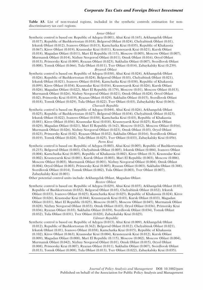
Corporate Tax Cuts and Foreign Direct Investment
Table A5. List of non-treated regions, included in the synthetic controls estimation for non-discriminatory tax cut1 regions.
Amur OblastSynthetic control is based on: Republic of Adygea (0.001), Altai Krai (0.165), Arkhangelsk Oblast
(0.017), Republic of Bashkortostan (0.018), Belgorod Oblast (0.024), Chelyabinsk Oblast (0.01),Irkutsk Oblast (0.012), Ivanovo Oblast (0.013), Kamchatka Krai (0.035), Republic of Khakassia(0.067), Kirov Oblast (0.019), Krasnodar Krai (0.011), Krasnoyarsk Krai (0.021), Kursk Oblast(0.018), Magadan Oblast (0.011), Mari El Republic (0.115), Moscow (0.005), Moscow Oblast (0.007),Murmansk Oblast (0.014), Nizhny Novgorod Oblast (0.011), Omsk Oblast (0.016), Oryol Oblast(0.013), Primorsky Krai (0.009), Ryazan Oblast (0.023), Sakhalin Oblast (0.007), Sverdlovsk Oblast(0.008), Tomsk Oblast (0.066), Tula Oblast (0.011), Tver Oblast (0.014), Zabaykalsky Krai (0.239).
Bryansk OblastSynthetic control is based on: Republic of Adygea (0.038), Altai Krai (0.024), Arkhangelsk Oblast
(0.026), Republic of Bashkortostan (0.024), Belgorod Oblast (0.03), Chelyabinsk Oblast (0.021),Irkutsk Oblast (0.021), Ivanovo Oblast (0.034), Kamchatka Krai (0.038), Republic of Khakassia(0.099), Kirov Oblast (0.034), Krasnodar Krai (0.016), Krasnoyarsk Krai (0.026), Kursk Oblast(0.026), Magadan Oblast (0.022), Mari El Republic (0.179), Moscow (0.01), Moscow Oblast (0.013),Murmansk Oblast (0.026), Nizhny Novgorod Oblast (0.021), Omsk Oblast (0.028), Oryol Oblast(0.02), Primorsky Krai (0.019), Ryazan Oblast (0.029), Sakhalin Oblast (0.015), Sverdlovsk Oblast(0.018), Tomsk Oblast (0.029), Tula Oblast (0.022), Tver Oblast (0.03), Zabaykalsky Krai (0.063).
Chuvash RepublicSynthetic control is based on: Republic of Adygea (0.044), Altai Krai (0.026), Arkhangelsk Oblast
(0.025), Republic of Bashkortostan (0.027), Belgorod Oblast (0.034), Chelyabinsk Oblast (0.023),Irkutsk Oblast (0.022), Ivanovo Oblast (0.038), Kamchatka Krai (0.03), Republic of Khakassia(0.081), Kirov Oblast (0.036), Krasnodar Krai (0.018), Krasnoyarsk Krai (0.025), Kursk Oblast(0.029), Magadan Oblast (0.021), Mari El Republic (0.162), Moscow (0.012), Moscow Oblast (0.016),Murmansk Oblast (0.026), Nizhny Novgorod Oblast (0.023), Omsk Oblast (0.03), Oryol Oblast(0.023), Primorsky Krai (0.02), Ryazan Oblast (0.032), Sakhalin Oblast (0.016), Sverdlovsk Oblast(0.019), Tomsk Oblast (0.028), Tula Oblast (0.025), Tver Oblast (0.033), Zabaykalsky Krai (0.056).
Perm KraiSynthetic control is based on: Republic of Adygea (0.003), Altai Krai (0.005), Republic of Bashkortostan
(0.215), Belgorod Oblast (0.003), Chelyabinsk Oblast (0.005), Irkutsk Oblast (0.004), Ivanovo Oblast(0.004), Kamchatka Krai (0.005), Republic of Khakassia (0.002), Kirov Oblast (0.3), Krasnodar Krai(0.002), Krasnoyarsk Krai (0.001), Kursk Oblast (0.003), Mari El Republic (0.003), Moscow (0.006),Moscow Oblast (0.003), Murmansk Oblast (0.001), Nizhny Novgorod Oblast (0.004), Omsk Oblast(0.004), Oryol Oblast (0.003), Primorsky Krai (0.005), Ryazan Oblast (0.003), Sakhalin Oblast (0.388),Sverdlovsk Oblast (0.014), Tomsk Oblast (0.002), Tula Oblast (0.003), Tver Oblast (0.007),Zabaykalsky Krai (0.001).
Other potential control units include: Arkhangelsk Oblast, Magadan Oblast.Rostov Oblast
Synthetic control is based on: Republic of Adygea (0.029), Altai Krai (0.035), Arkhangelsk Oblast (0.03),Republic of Bashkortostan (0.032), Belgorod Oblast (0.03), Chelyabinsk Oblast (0.032), IrkutskOblast (0.033), Ivanovo Oblast (0.025), Kamchatka Krai (0.025), Republic of Khakassia (0.024), KirovOblast (0.026), Krasnodar Krai (0.044), Krasnoyarsk Krai (0.03), Kursk Oblast (0.033), MagadanOblast (0.031), Mari El Republic (0.025), Moscow (0.087), Moscow Oblast (0.045), Murmansk Oblast(0.028), Nizhny Novgorod Oblast (0.033), Omsk Oblast (0.03), Oryol Oblast (0.036), Primorsky Krai(0.036), Ryazan Oblast (0.03), Sakhalin Oblast (0.039), Sverdlovsk Oblast (0.034), Tomsk Oblast(0.032), Tula Oblast (0.031), Tver Oblast (0.028), Zabaykalsky Krai (0.025).
Udmurt RepublicSynthetic control is based on: Republic of Adygea (0.013), Altai Krai (0.009), Arkhangelsk Oblast
(0.012), Republic of Bashkortostan (0.362), Belgorod Oblast (0.012), Chelyabinsk Oblast (0.021),Irkutsk Oblast (0.01), Ivanovo Oblast (0.038), Kamchatka Krai (0.015), Republic of Khakassia(0.102), Kirov Oblast (0.063), Krasnodar Krai (0.004), Krasnoyarsk Krai (0.012), Kursk Oblast(0.009), Magadan Oblast (0.008), Mari El Republic (0.115), Moscow (0.002), Moscow Oblast (0.004),Murmansk Oblast (0.042), Nizhny Novgorod Oblast (0.01), Omsk Oblast (0.015), Oryol Oblast(0.008), Primorsky Krai (0.007), Ryazan Oblast (0.011), Sakhalin Oblast (0.007), Sverdlovsk Oblast(0.013), Tomsk Oblast (0.008), Tula Oblast (0.013), Tver Oblast (0.022), Zabaykalsky Krai (0.035).
Journal of Policy Analysis and Management DOI: 10.1002/pamPublished on behalf of the Association for Public Policy Analysis and Management

Corporate Tax Cuts and Foreign Direct Investment
Table A6. List of non-treated regions, included in the synthetic controls estimation for dis-criminatory tax cut1 regions.
Altai RepublicSynthetic control is based on: Republic of Adygea (0.013), Altai Krai (0.009), Arkhangelsk
Oblast (0.012), Republic of Bashkortostan (0.362), Belgorod Oblast (0.012), ChelyabinskOblast (0.021), Irkutsk Oblast (0.01), Ivanovo Oblast (0.038), Kamchatka Krai (0.015),Republic of Khakassia (0.102), Kirov Oblast (0.063), Krasnodar Krai (0.004), KrasnoyarskKrai (0.012), Kursk Oblast (0.009), Magadan Oblast (0.008), Mari El Republic (0.115),Moscow (0.002), Moscow Oblast (0.004), Murmansk Oblast (0.042), Nizhny NovgorodOblast (0.01), Omsk Oblast (0.015), Oryol Oblast (0.008), Primorsky Krai (0.007), RyazanOblast (0.011), Sakhalin Oblast (0.007), Sverdlovsk Oblast (0.013), Tomsk Oblast (0.008),Tula Oblast (0.013), Tver Oblast (0.022), Zabaykalsky Krai (0.035).
Astrakhan OblastSynthetic control is based on: Republic of Adygea (0.041), Altai Krai (0.025), Arkhangelsk
Oblast (0.026), Republic of Bashkortostan (0.025), Belgorod Oblast (0.031), ChelyabinskOblast (0.021), Irkutsk Oblast (0.022), Ivanovo Oblast (0.034), Kamchatka Krai (0.043),Republic of Khakassia (0.093), Kirov Oblast (0.035), Krasnodar Krai (0.017), KrasnoyarskKrai (0.027), Kursk Oblast (0.028), Magadan Oblast (0.026), Mari El Republic (0.147),Moscow (0.011), Moscow Oblast (0.014), Murmansk Oblast (0.026), Nizhny NovgorodOblast (0.022), Omsk Oblast (0.029), Oryol Oblast (0.022), Primorsky Krai (0.02), RyazanOblast (0.03), Sakhalin Oblast (0.016), Sverdlovsk Oblast (0.018), Tomsk Oblast (0.03),Tula Oblast (0.023), Tver Oblast (0.032), Zabaykalsky Krai (0.065).
Republic of DagestanSynthetic control is based on: Republic of Adygea (0.02), Altai Krai (0.008), Arkhangelsk
Oblast (0.006), Republic of Bashkortostan (0.009), Belgorod Oblast (0.015), ChelyabinskOblast (0.006), Irkutsk Oblast (0.005), Ivanovo Oblast (0.014), Kamchatka Krai (0.007),Republic of Khakassia (0.031), Kirov Oblast (0.011), Krasnodar Krai (0.004), KrasnoyarskKrai (0.006), Kursk Oblast (0.011), Magadan Oblast (0.005), Mari El Republic (0.746),Moscow (0.002), Moscow Oblast (0.004), Murmansk Oblast (0.006), Nizhny NovgorodOblast (0.007), Omsk Oblast (0.009), Oryol Oblast (0.007), Primorsky Krai (0.005),Ryazan Oblast (0.011), Sakhalin Oblast (0.003), Sverdlovsk Oblast (0.005), Tomsk Oblast(0.007), Tula Oblast (0.008), Tver Oblast (0.013), Zabaykalsky Krai (0.01).
Kaluga OblastSynthetic control is based on: Republic of Adygea (0.025), Altai Krai (0.032), Arkhangelsk
Oblast (0.03), Republic of Bashkortostan (0.031), Belgorod Oblast (0.028), ChelyabinskOblast (0.034), Irkutsk Oblast (0.033), Ivanovo Oblast (0.026), Kamchatka Krai (0.025),Republic of Khakassia (0.022), Kirov Oblast (0.026), Krasnodar Krai (0.041), KrasnoyarskKrai (0.03), Kursk Oblast (0.03), Magadan Oblast (0.033), Mari El Republic (0.021),Moscow (0.106), Moscow Oblast (0.046), Murmansk Oblast (0.03), Nizhny NovgorodOblast (0.034), Omsk Oblast (0.029), Oryol Oblast (0.035), Primorsky Krai (0.036),Ryazan Oblast (0.028), Sakhalin Oblast (0.043), Sverdlovsk Oblast (0.037), Tomsk Oblast(0.028), Tula Oblast (0.033), Tver Oblast (0.028), Zabaykalsky Krai (0.022).
Republic of KareliaSynthetic control is based on: Republic of Adygea (0.004), Altai Krai (0.012), Arkhangelsk
Oblast (0.009), Republic of Bashkortostan (0.126), Belgorod Oblast (0.003), ChelyabinskOblast (0.015), Irkutsk Oblast (0.007), Ivanovo Oblast (0.005), Kamchatka Krai (0.001),Republic of Khakassia (0.004), Kirov Oblast (0.019), Krasnodar Krai (0.007), KrasnoyarskKrai (0.007), Kursk Oblast (0.004), Magadan Oblast (0.002), Mari El Republic (0.005),Moscow Oblast (0.002), Murmansk Oblast (0.004), Nizhny Novgorod Oblast (0.004),Omsk Oblast (0.01), Oryol Oblast (0.004), Primorsky Krai (0.004), Ryazan Oblast (0.003),Sakhalin Oblast (0.375), Sverdlovsk Oblast (0.038), Tomsk Oblast (0.003), Tula Oblast(0.005), Tver Oblast (0.014), Zabaykalsky Krai (0.305).
Other potential control units include: Moscow.
Journal of Policy Analysis and Management DOI: 10.1002/pamPublished on behalf of the Association for Public Policy Analysis and Management
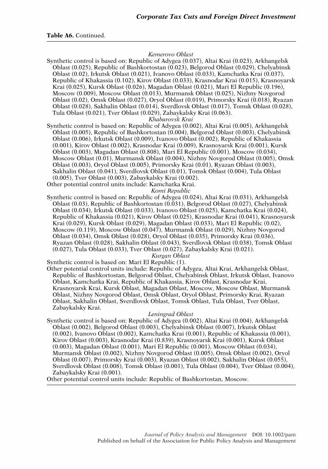
Corporate Tax Cuts and Foreign Direct Investment
Table A6. Continued.
Kemerovo OblastSynthetic control is based on: Republic of Adygea (0.037), Altai Krai (0.023), Arkhangelsk
Oblast (0.025), Republic of Bashkortostan (0.023), Belgorod Oblast (0.029), ChelyabinskOblast (0.02), Irkutsk Oblast (0.021), Ivanovo Oblast (0.033), Kamchatka Krai (0.037),Republic of Khakassia (0.102), Kirov Oblast (0.033), Krasnodar Krai (0.015), KrasnoyarskKrai (0.025), Kursk Oblast (0.026), Magadan Oblast (0.021), Mari El Republic (0.196),Moscow (0.009), Moscow Oblast (0.013), Murmansk Oblast (0.025), Nizhny NovgorodOblast (0.02), Omsk Oblast (0.027), Oryol Oblast (0.019), Primorsky Krai (0.018), RyazanOblast (0.028), Sakhalin Oblast (0.014), Sverdlovsk Oblast (0.017), Tomsk Oblast (0.028),Tula Oblast (0.021), Tver Oblast (0.029), Zabaykalsky Krai (0.063).
Khabarovsk KraiSynthetic control is based on: Republic of Adygea (0.002), Altai Krai (0.005), Arkhangelsk
Oblast (0.005), Republic of Bashkortostan (0.004), Belgorod Oblast (0.003), ChelyabinskOblast (0.006), Irkutsk Oblast (0.009), Ivanovo Oblast (0.002), Republic of Khakassia(0.001), Kirov Oblast (0.002), Krasnodar Krai (0.009), Krasnoyarsk Krai (0.001), KurskOblast (0.003), Magadan Oblast (0.808), Mari El Republic (0.001), Moscow (0.034),Moscow Oblast (0.01), Murmansk Oblast (0.004), Nizhny Novgorod Oblast (0.005), OmskOblast (0.003), Oryol Oblast (0.005), Primorsky Krai (0.01), Ryazan Oblast (0.003),Sakhalin Oblast (0.041), Sverdlovsk Oblast (0.01), Tomsk Oblast (0.004), Tula Oblast(0.005), Tver Oblast (0.003), Zabaykalsky Krai (0.002).
Other potential control units include: Kamchatka Krai.Komi Republic
Synthetic control is based on: Republic of Adygea (0.024), Altai Krai (0.031), ArkhangelskOblast (0.03), Republic of Bashkortostan (0.031), Belgorod Oblast (0.027), ChelyabinskOblast (0.034), Irkutsk Oblast (0.033), Ivanovo Oblast (0.025), Kamchatka Krai (0.024),Republic of Khakassia (0.021), Kirov Oblast (0.025), Krasnodar Krai (0.041), KrasnoyarskKrai (0.029), Kursk Oblast (0.029), Magadan Oblast (0.033), Mari El Republic (0.02),Moscow (0.119), Moscow Oblast (0.047), Murmansk Oblast (0.029), Nizhny NovgorodOblast (0.034), Omsk Oblast (0.028), Oryol Oblast (0.035), Primorsky Krai (0.036),Ryazan Oblast (0.028), Sakhalin Oblast (0.043), Sverdlovsk Oblast (0.038), Tomsk Oblast(0.027), Tula Oblast (0.033), Tver Oblast (0.027), Zabaykalsky Krai (0.021).
Kurgan OblastSynthetic control is based on: Mari El Republic (1).Other potential control units include: Republic of Adygea, Altai Krai, Arkhangelsk Oblast,
Republic of Bashkortostan, Belgorod Oblast, Chelyabinsk Oblast, Irkutsk Oblast, IvanovoOblast, Kamchatka Krai, Republic of Khakassia, Kirov Oblast, Krasnodar Krai,Krasnoyarsk Krai, Kursk Oblast, Magadan Oblast, Moscow, Moscow Oblast, MurmanskOblast, Nizhny Novgorod Oblast, Omsk Oblast, Oryol Oblast, Primorsky Krai, RyazanOblast, Sakhalin Oblast, Sverdlovsk Oblast, Tomsk Oblast, Tula Oblast, Tver Oblast,Zabaykalsky Krai.
Leningrad OblastSynthetic control is based on: Republic of Adygea (0.002), Altai Krai (0.004), Arkhangelsk
Oblast (0.002), Belgorod Oblast (0.003), Chelyabinsk Oblast (0.007), Irkutsk Oblast(0.002), Ivanovo Oblast (0.002), Kamchatka Krai (0.001), Republic of Khakassia (0.001),Kirov Oblast (0.003), Krasnodar Krai (0.839), Krasnoyarsk Krai (0.001), Kursk Oblast(0.003), Magadan Oblast (0.001), Mari El Republic (0.001), Moscow Oblast (0.034),Murmansk Oblast (0.002), Nizhny Novgorod Oblast (0.005), Omsk Oblast (0.002), OryolOblast (0.007), Primorsky Krai (0.003), Ryazan Oblast (0.002), Sakhalin Oblast (0.055),Sverdlovsk Oblast (0.008), Tomsk Oblast (0.001), Tula Oblast (0.004), Tver Oblast (0.004),Zabaykalsky Krai (0.001).
Other potential control units include: Republic of Bashkortostan, Moscow.
Journal of Policy Analysis and Management DOI: 10.1002/pamPublished on behalf of the Association for Public Policy Analysis and Management
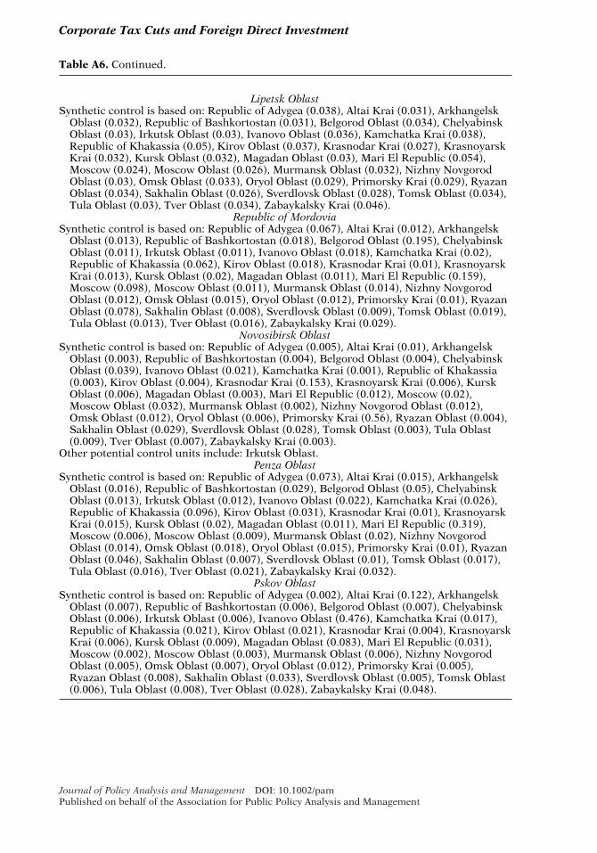
Corporate Tax Cuts and Foreign Direct Investment
Table A6. Continued.
Lipetsk OblastSynthetic control is based on: Republic of Adygea (0.038), Altai Krai (0.031), Arkhangelsk
Oblast (0.032), Republic of Bashkortostan (0.031), Belgorod Oblast (0.034), ChelyabinskOblast (0.03), Irkutsk Oblast (0.03), Ivanovo Oblast (0.036), Kamchatka Krai (0.038),Republic of Khakassia (0.05), Kirov Oblast (0.037), Krasnodar Krai (0.027), KrasnoyarskKrai (0.032), Kursk Oblast (0.032), Magadan Oblast (0.03), Mari El Republic (0.054),Moscow (0.024), Moscow Oblast (0.026), Murmansk Oblast (0.032), Nizhny NovgorodOblast (0.03), Omsk Oblast (0.033), Oryol Oblast (0.029), Primorsky Krai (0.029), RyazanOblast (0.034), Sakhalin Oblast (0.026), Sverdlovsk Oblast (0.028), Tomsk Oblast (0.034),Tula Oblast (0.03), Tver Oblast (0.034), Zabaykalsky Krai (0.046).
Republic of MordoviaSynthetic control is based on: Republic of Adygea (0.067), Altai Krai (0.012), Arkhangelsk
Oblast (0.013), Republic of Bashkortostan (0.018), Belgorod Oblast (0.195), ChelyabinskOblast (0.011), Irkutsk Oblast (0.011), Ivanovo Oblast (0.018), Kamchatka Krai (0.02),Republic of Khakassia (0.062), Kirov Oblast (0.018), Krasnodar Krai (0.01), KrasnoyarskKrai (0.013), Kursk Oblast (0.02), Magadan Oblast (0.011), Mari El Republic (0.159),Moscow (0.098), Moscow Oblast (0.011), Murmansk Oblast (0.014), Nizhny NovgorodOblast (0.012), Omsk Oblast (0.015), Oryol Oblast (0.012), Primorsky Krai (0.01), RyazanOblast (0.078), Sakhalin Oblast (0.008), Sverdlovsk Oblast (0.009), Tomsk Oblast (0.019),Tula Oblast (0.013), Tver Oblast (0.016), Zabaykalsky Krai (0.029).
Novosibirsk OblastSynthetic control is based on: Republic of Adygea (0.005), Altai Krai (0.01), Arkhangelsk
Oblast (0.003), Republic of Bashkortostan (0.004), Belgorod Oblast (0.004), ChelyabinskOblast (0.039), Ivanovo Oblast (0.021), Kamchatka Krai (0.001), Republic of Khakassia(0.003), Kirov Oblast (0.004), Krasnodar Krai (0.153), Krasnoyarsk Krai (0.006), KurskOblast (0.006), Magadan Oblast (0.003), Mari El Republic (0.012), Moscow (0.02),Moscow Oblast (0.032), Murmansk Oblast (0.002), Nizhny Novgorod Oblast (0.012),Omsk Oblast (0.012), Oryol Oblast (0.006), Primorsky Krai (0.56), Ryazan Oblast (0.004),Sakhalin Oblast (0.029), Sverdlovsk Oblast (0.028), Tomsk Oblast (0.003), Tula Oblast(0.009), Tver Oblast (0.007), Zabaykalsky Krai (0.003).
Other potential control units include: Irkutsk Oblast.Penza Oblast
Synthetic control is based on: Republic of Adygea (0.073), Altai Krai (0.015), ArkhangelskOblast (0.016), Republic of Bashkortostan (0.029), Belgorod Oblast (0.05), ChelyabinskOblast (0.013), Irkutsk Oblast (0.012), Ivanovo Oblast (0.022), Kamchatka Krai (0.026),Republic of Khakassia (0.096), Kirov Oblast (0.031), Krasnodar Krai (0.01), KrasnoyarskKrai (0.015), Kursk Oblast (0.02), Magadan Oblast (0.011), Mari El Republic (0.319),Moscow (0.006), Moscow Oblast (0.009), Murmansk Oblast (0.02), Nizhny NovgorodOblast (0.014), Omsk Oblast (0.018), Oryol Oblast (0.015), Primorsky Krai (0.01), RyazanOblast (0.046), Sakhalin Oblast (0.007), Sverdlovsk Oblast (0.01), Tomsk Oblast (0.017),Tula Oblast (0.016), Tver Oblast (0.021), Zabaykalsky Krai (0.032).
Pskov OblastSynthetic control is based on: Republic of Adygea (0.002), Altai Krai (0.122), Arkhangelsk
Oblast (0.007), Republic of Bashkortostan (0.006), Belgorod Oblast (0.007), ChelyabinskOblast (0.006), Irkutsk Oblast (0.006), Ivanovo Oblast (0.476), Kamchatka Krai (0.017),Republic of Khakassia (0.021), Kirov Oblast (0.021), Krasnodar Krai (0.004), KrasnoyarskKrai (0.006), Kursk Oblast (0.009), Magadan Oblast (0.083), Mari El Republic (0.031),Moscow (0.002), Moscow Oblast (0.003), Murmansk Oblast (0.006), Nizhny NovgorodOblast (0.005), Omsk Oblast (0.007), Oryol Oblast (0.012), Primorsky Krai (0.005),Ryazan Oblast (0.008), Sakhalin Oblast (0.033), Sverdlovsk Oblast (0.005), Tomsk Oblast(0.006), Tula Oblast (0.008), Tver Oblast (0.028), Zabaykalsky Krai (0.048).
Journal of Policy Analysis and Management DOI: 10.1002/pamPublished on behalf of the Association for Public Policy Analysis and Management

Corporate Tax Cuts and Foreign Direct Investment
Table A6. Continued.
Smolensk OblastSynthetic control is based on: Republic of Adygea (0.166), Altai Krai (0.001), Arkhangelsk
Oblast (0.001), Republic of Bashkortostan (0.002), Belgorod Oblast (0.005), ChelyabinskOblast (0.001), Irkutsk Oblast (0.001), Ivanovo Oblast (0.007), Kamchatka Krai (0.002),Republic of Khakassia (0.121), Kirov Oblast (0.004), Krasnodar Krai (0.001), KrasnoyarskKrai (0.001), Kursk Oblast (0.004), Magadan Oblast (0.09), Mari El Republic (0.565),Moscow (0.001), Moscow Oblast (0.001), Murmansk Oblast (0.002), Nizhny NovgorodOblast (0.002), Omsk Oblast (0.002), Oryol Oblast (0.002), Primorsky Krai (0.001),Ryazan Oblast (0.004), Sakhalin Oblast (0.001), Sverdlovsk Oblast (0.001), Tomsk Oblast(0.001), Tula Oblast (0.002), Tver Oblast (0.008).
Other potential control units include: Zabaykalsky Krai.Stavropol Krai
Synthetic control is based on: Republic of Adygea (0.02), Altai Krai (0.03), ArkhangelskOblast (0.028), Republic of Bashkortostan (0.029), Belgorod Oblast (0.024), ChelyabinskOblast (0.033), Irkutsk Oblast (0.032), Ivanovo Oblast (0.022), Kamchatka Krai (0.02),Republic of Khakassia (0.017), Kirov Oblast (0.022), Krasnodar Krai (0.042), KrasnoyarskKrai (0.027), Kursk Oblast (0.027), Magadan Oblast (0.032), Mari El Republic (0.016),Moscow (0.167), Moscow Oblast (0.048), Murmansk Oblast (0.027), Nizhny NovgorodOblast (0.033), Omsk Oblast (0.026), Oryol Oblast (0.034), Primorsky Krai (0.036),Ryazan Oblast (0.025), Sakhalin Oblast (0.044), Sverdlovsk Oblast (0.038), Tomsk Oblast(0.025), Tula Oblast (0.032), Tver Oblast (0.024), Zabaykalsky Krai (0.017).
Tambov OblastSynthetic control is based on: Republic of Adygea (0.645), Altai Krai (0.003), Arkhangelsk
Oblast (0.004), Republic of Bashkortostan (0.003), Belgorod Oblast (0.117), ChelyabinskOblast (0.003), Irkutsk Oblast (0.003), Ivanovo Oblast (0.005), Kamchatka Krai (0.007),Republic of Khakassia (0.014), Kirov Oblast (0.006), Krasnodar Krai (0.002), KrasnoyarskKrai (0.004), Kursk Oblast (0.004), Magadan Oblast (0.003), Mari El Republic (0.017),Moscow (0.001), Moscow Oblast (0.002), Murmansk Oblast (0.004), Nizhny NovgorodOblast (0.003), Omsk Oblast (0.004), Oryol Oblast (0.003), Primorsky Krai (0.002),Ryazan Oblast (0.119), Sakhalin Oblast (0.002), Sverdlovsk Oblast (0.002), Tomsk Oblast(0.004), Tula Oblast (0.003), Tver Oblast (0.005), Zabaykalsky Krai (0.007).
Republic of TatarstanSynthetic control is based on: Republic of Adygea (0.001), Altai Krai (0.002), Arkhangelsk
Oblast (0.003), Republic of Bashkortostan (0.571), Belgorod Oblast (0.002), ChelyabinskOblast (0.019), Irkutsk Oblast (0.006), Ivanovo Oblast (0.001), Kamchatka Krai (0.002),Republic of Khakassia (0.095), Kirov Oblast (0.003), Krasnodar Krai (0.003), KrasnoyarskKrai (0.009), Kursk Oblast (0.003), Magadan Oblast (0.006), Moscow (0.144), MoscowOblast (0.003), Murmansk Oblast (0.007), Nizhny Novgorod Oblast (0.006), Omsk Oblast(0.006), Oryol Oblast (0.002), Primorsky Krai (0.004), Ryazan Oblast (0.001), SakhalinOblast (0.047), Sverdlovsk Oblast (0.032), Tomsk Oblast (0.002), Tula Oblast (0.003), TverOblast (0.017), Zabaykalsky Krai (0.002).
Other potential control units include: Mari El Republic.Tyumen Oblast
Synthetic control is based on: Republic of Adygea (0.004), Altai Krai (0.01), ArkhangelskOblast (0.025), Republic of Bashkortostan (0.013), Belgorod Oblast (0.005), ChelyabinskOblast (0.017), Irkutsk Oblast (0.023), Ivanovo Oblast (0.005), Kamchatka Krai (0.001),Republic of Khakassia (0.003), Kirov Oblast (0.006), Krasnodar Krai (0.023), KrasnoyarskKrai (0.434), Kursk Oblast (0.006), Mari El Republic (0.003), Moscow (0.027), MoscowOblast (0.014), Murmansk Oblast (0.017), Nizhny Novgorod Oblast (0.01), Omsk Oblast(0.008), Oryol Oblast (0.01), Primorsky Krai (0.015), Ryazan Oblast (0.006), SakhalinOblast (0.243), Sverdlovsk Oblast (0.043), Tomsk Oblast (0.006), Tula Oblast (0.011), TverOblast (0.006), Zabaykalsky Krai (0.003).
Other potential control units include: Magadan Oblast.
Journal of Policy Analysis and Management DOI: 10.1002/pamPublished on behalf of the Association for Public Policy Analysis and Management
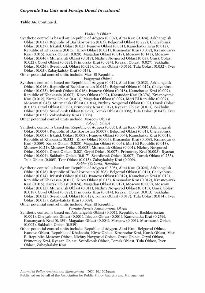
Corporate Tax Cuts and Foreign Direct Investment
Table A6. Continued.
Vladimir OblastSynthetic control is based on: Republic of Adygea (0.007), Altai Krai (0.024), Arkhangelsk
Oblast (0.017), Republic of Bashkortostan (0.03), Belgorod Oblast (0.222), ChelyabinskOblast (0.027), Irkutsk Oblast (0.02), Ivanovo Oblast (0.031), Kamchatka Krai (0.012),Republic of Khakassia (0.015), Kirov Oblast (0.021), Krasnodar Krai (0.032), KrasnoyarskKrai (0.015), Kursk Oblast (0.029), Magadan Oblast (0.017), Moscow (0.143), MoscowOblast (0.046), Murmansk Oblast (0.017), Nizhny Novgorod Oblast (0.03), Omsk Oblast(0.022), Oryol Oblast (0.028), Primorsky Krai (0.024), Ryazan Oblast (0.027), SakhalinOblast (0.026), Sverdlovsk Oblast (0.026), Tomsk Oblast (0.016), Tula Oblast (0.032), TverOblast (0.03), Zabaykalsky Krai (0.013).
Other potential control units include: Mari El Republic.Volgograd Oblast
Synthetic control is based on: Republic of Adygea (0.012), Altai Krai (0.032), ArkhangelskOblast (0.016), Republic of Bashkortostan (0.042), Belgorod Oblast (0.012), ChelyabinskOblast (0.035), Irkutsk Oblast (0.016), Ivanovo Oblast (0.018), Kamchatka Krai (0.007),Republic of Khakassia (0.007), Kirov Oblast (0.02), Krasnodar Krai (0.376), KrasnoyarskKrai (0.012), Kursk Oblast (0.013), Magadan Oblast (0.007), Mari El Republic (0.007),Moscow (0.043), Murmansk Oblast (0.014), Nizhny Novgorod Oblast (0.02), Omsk Oblast(0.015), Oryol Oblast (0.033), Primorsky Krai (0.017), Ryazan Oblast (0.013), SakhalinOblast (0.058), Sverdlovsk Oblast (0.069), Tomsk Oblast (0.008), Tula Oblast (0.047), TverOblast (0.023), Zabaykalsky Krai (0.008).
Other potential control units include: Moscow Oblast.Vologda Oblast
Synthetic control is based on: Republic of Adygea (0.005), Altai Krai (0.009), ArkhangelskOblast (0.004), Republic of Bashkortostan (0.007), Belgorod Oblast (0.01), ChelyabinskOblast (0.008), Irkutsk Oblast (0.008), Ivanovo Oblast (0.004), Kamchatka Krai (0.001),Republic of Khakassia (0.332), Kirov Oblast (0.005), Krasnodar Krai (0.008), KrasnoyarskKrai (0.009), Kursk Oblast (0.025), Magadan Oblast (0.005), Mari El Republic (0.013),Moscow (0.21), Moscow Oblast (0.005), Murmansk Oblast (0.001), Nizhny NovgorodOblast (0.009), Omsk Oblast (0.02), Oryol Oblast (0.007), Primorsky Krai (0.008), RyazanOblast (0.004), Sakhalin Oblast (0.017), Sverdlovsk Oblast (0.007), Tomsk Oblast (0.233),Tula Oblast (0.005), Tver Oblast (0.013), Zabaykalsky Krai (0.009).
Sakha (Yakutia) RepublicSynthetic control is based on: Republic of Adygea (0.305), Altai Krai (0.024), Arkhangelsk
Oblast (0.016), Republic of Bashkortostan (0.306), Belgorod Oblast (0.014), ChelyabinskOblast (0.014), Irkutsk Oblast (0.014), Ivanovo Oblast (0.012), Kamchatka Krai (0.012),Republic of Khakassia (0.011), Kirov Oblast (0.015), Krasnodar Krai (0.012), KrasnoyarskKrai (0.015), Kursk Oblast (0.024), Magadan Oblast (0.012), Moscow (0.009), MoscowOblast (0.012), Murmansk Oblast (0.011), Nizhny Novgorod Oblast (0.015), Omsk Oblast(0.018), Oryol Oblast (0.022), Primorsky Krai (0.014), Ryazan Oblast (0.013), SakhalinOblast (0.012), Sverdlovsk Oblast (0.012), Tomsk Oblast (0.017), Tula Oblast (0.014), TverOblast (0.015), Zabaykalsky Krai (0.009).
Other potential control units include: Mari El Republic.Yamalo-Nenets Autonomous Okrug
Synthetic control is based on: Arkhangelsk Oblast (0.001), Republic of Bashkortostan(0.001), Chelyabinsk Oblast (0.001), Irkutsk Oblast (0.001), Kamchatka Krai (0.256),Krasnoyarsk Krai (0.189), Magadan Oblast (0.004), Moscow (0.001), Murmansk Oblast(0.002), Sakhalin Oblast (0.539).
Other potential control units include: Republic of Adygea, Altai Krai, Belgorod Oblast,Ivanovo Oblast, Republic of Khakassia, Kirov Oblast, Krasnodar Krai, Kursk Oblast, MariEl Republic, Moscow Oblast, Nizhny Novgorod Oblast, Omsk Oblast, Oryol Oblast,Primorsky Krai, Ryazan Oblast, Sverdlovsk Oblast, Tomsk Oblast, Tula Oblast, TverOblast, Zabaykalsky Krai.
Journal of Policy Analysis and Management DOI: 10.1002/pamPublished on behalf of the Association for Public Policy Analysis and Management

Corporate Tax Cuts and Foreign Direct Investment
Table A6. Continued.
Yaroslavl OblastSynthetic control is based on: Republic of Adygea (0.028), Altai Krai (0.031), Arkhangelsk
Oblast (0.032), Republic of Bashkortostan (0.03), Belgorod Oblast (0.028), ChelyabinskOblast (0.037), Irkutsk Oblast (0.034), Ivanovo Oblast (0.039), Kamchatka Krai (0.021),Republic of Khakassia (0.025), Kirov Oblast (0.03), Krasnodar Krai (0.031), KrasnoyarskKrai (0.031), Kursk Oblast (0.029), Magadan Oblast (0.023), Mari El Republic (0.121),Moscow (0.03), Moscow Oblast (0.03), Murmansk Oblast (0.03), Nizhny Novgorod Oblast(0.033), Omsk Oblast (0.038), Oryol Oblast (0.026), Primorsky Krai (0.033), RyazanOblast (0.025), Sakhalin Oblast (0.026), Sverdlovsk Oblast (0.034), Tomsk Oblast (0.033),Tula Oblast (0.031), Tver Oblast (0.032), Zabaykalsky Krai (0.031).
Journal of Policy Analysis and Management DOI: 10.1002/pamPublished on behalf of the Association for Public Policy Analysis and Management

Corporate Tax Cuts and Foreign Direct Investment
Figure A1. Synthetic control analysis for discriminatory tax cut1 regions.
Journal of Policy Analysis and Management DOI: 10.1002/pamPublished on behalf of the Association for Public Policy Analysis and Management

Corporate Tax Cuts and Foreign Direct Investment
Figure A1. continued.
Journal of Policy Analysis and Management DOI: 10.1002/pamPublished on behalf of the Association for Public Policy Analysis and Management
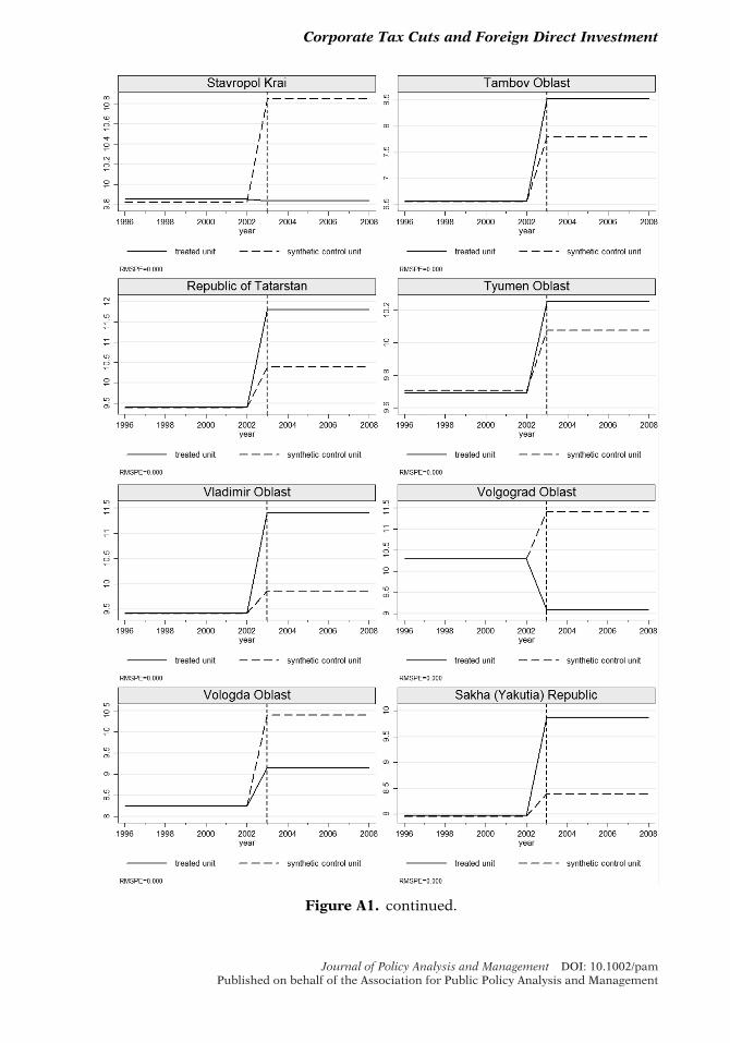
Corporate Tax Cuts and Foreign Direct Investment
Figure A1. continued.
Journal of Policy Analysis and Management DOI: 10.1002/pamPublished on behalf of the Association for Public Policy Analysis and Management
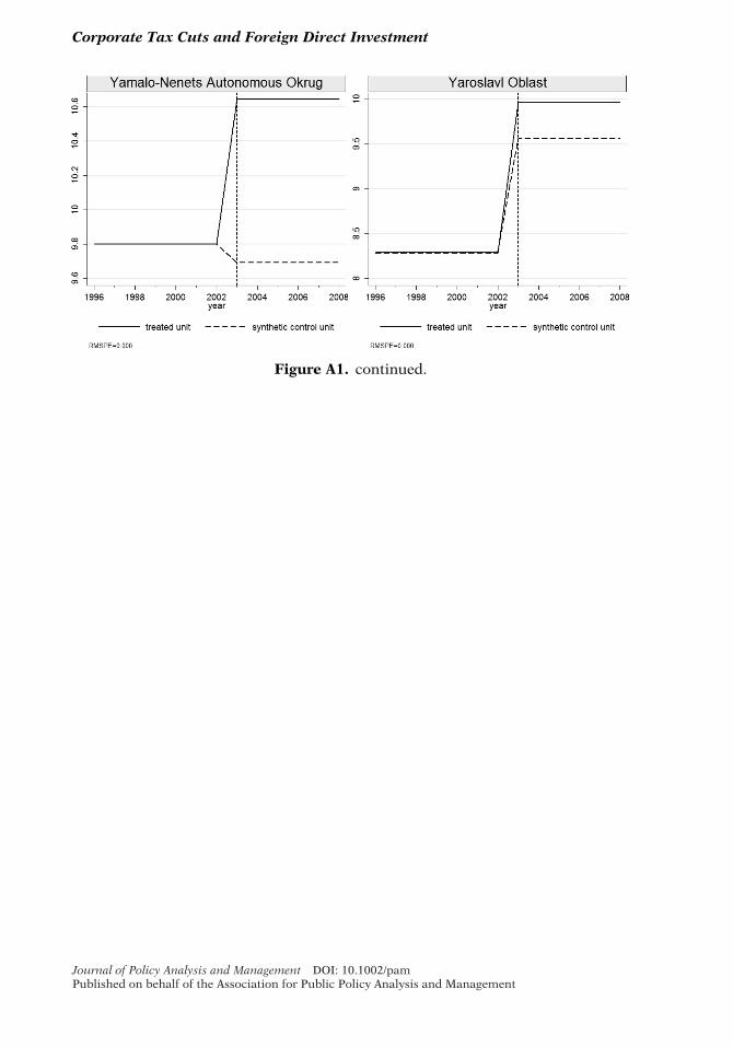
Corporate Tax Cuts and Foreign Direct Investment
Figure A1. continued.
Journal of Policy Analysis and Management DOI: 10.1002/pamPublished on behalf of the Association for Public Policy Analysis and Management