Corporate Investment and Asset Price Dynamics:Implications for the Cross Section of Returns

Murray Carlson, Adlai Fisher, and Ron Giammarino∗

The University of British Columbia

First Draft: February 2002This Draft: May 7, 2003

∗2053 Main Mall, Vancouver, BC, V6T 1Z2 Canada, murray.carlson@commerce.ubc.ca, ad-lai.fisher@commerce.ubc.ca, ron.giammarino@commerce.ubc.ca. We appreciate helpful com-ments from Peter Christoffersen, Rob Heinkel, Burton Hollifield, Ali Lazrak, Rick Green, Ed-uardo Schwartz, Raman Uppal, Tan Wang, Yong Wang, Robert Whitelaw, an anonymous ref-eree, and seminar participants at the University of Alberta, UBC, and the 2003 conference onSimulation Based and Finite Sample Inference in Finance. Support for this project from thethe Bureau of Asset Management at UBC and the Social Sciences and Humanities ResearchCouncil of Canada (grant number 410-2003-0741) is gratefully acknowledged.

Corporate Investment and Asset Price Dynamics:Implications for the Cross Section of Returns

Abstract

We show that corporate investment decisions can explain conditionaldynamics in expected asset returns. Our approach is similar in spirit toBerk, Green, and Naik (1999), but we introduce to the investment problemoperating leverage, reversible real options, fixed adjustment costs, and finitegrowth opportunities. We assume constant revenue betas, but still obtainasset betas that vary through time as a reflection of historical investmentdecisions and product market demand. Book-to-market effects emerge andrelate to operating leverage, while size captures the importance of growthoptions relative to assets in place. We first develop these results in a simplesetting that permits closed-form solutions. Next, we empirically evaluate amore realistic specification that is solved numerically and estimated usingsimulated method of moments. This provides new quantitative evidenceon the importance of operating leverage and growth options to the cross-section of returns.

1. Introduction

Corporate investment decisions are often evaluated in a real options context,1 andoption exercise can change the riskiness of a firm in various ways. For example, ifgrowth opportunities are finite, the decision to invest changes the ratio of growthoptions to assets in place. Additionally, the resulting increase in physical capitalmay generate operating leverage through long-term obligations, including the fixedoperating costs of a larger plant, wage contracts, and commitments to suppliers. Itis natural to conclude that expected returns might relate to current and historicalinvestment decisions of the firm.

The empirical literature has long recognized a need to account for the dynamicstructure of risk when testing asset pricing models.2 A small but growing litera-ture that endogenizes expected returns through firm-level decisions has begun toprovide theoretical structure for risk and return dynamics. Motivated by assetprice anomalies,3 Berk, Green and Naik (“BGN”, 1999) were among the first toestablish a link between investment decisions, the riskiness of assets-in-place, andexpected return.4 Their model assumes that investment opportunities are hetero-geneous in risk. This would typically make cumbersome a complete descriptionof firm assets, but their model simplifies so that size and book-to-market aresufficient statistics for the aggregate risk of assets in place.

We contribute to this line of research by developing two dynamic models.These differ in their technical details, but rely on the same economic forces torelate endogenous firm investment to expected return. We arrive at a new eco-nomic role for operating leverage in explaining the book-to-market effect. Whendemand for a firm’s product decreases, equity value falls relative to the capitalstock, proxied by book value. Assuming fixed operating costs proportional to cap-ital, the riskiness of returns increases due to greater operating leverage. We also

1This approach was pioneered by McDonald and Siegel (1985, 1986) and Brennan andSchwartz (1986), and has been extended in many directions. See Dixit and Pindyck (1994)for a detailed analysis of the literature.

2Hansen and Richard (1987) make this point theoretically. To address the issue, typicalapplications use empirically or theoretically motivated instruments as conditioning variables.Two examples are Jagannathan and Wang (1996) and Ferson and Harvey (1999). Cochrane(2001) provides further discussion.

3Fama and French (1992) provide summary evidence on the ability of size and book-to-marketto explain returns. There is some debate as to whether this is due to factor risks (Fama andFrench, 1993) or priced characteristics (Daniel and Titman, 1998).

4Further work in this area includes Gomes, Kogan, and Zhang (2002), Zhang (2003), andCooper (2003).

1

incorporate limits to growth in both our models, and show that this is importantto obtaining an independent size effect. Our first model permits closed-form so-lutions in a stylized setting, allowing us to examine the relationship between sizeand book-to-market for a single firm. The second uses more realistic assumptionsand gives stationary dynamics for a cross-section of firms. This permits structuralestimation using the simulated method of moments.

In the first model, a single all-equity firm faces stochastic iso-elastic demandin its output market. The unique exogenous state variable is the demand level,driven by a lognormal diffusion. The firm may expand capacity a finite number oftimes, and a fixed adjustment cost is incurred each time operations are expanded.Operating leverage results from per-period fixed operating costs that increase inthe capital level. The underlying revenue betas are assumed constant, but firmbetas are nonetheless time-varying and reflect historical investment as well ascurrent demand.

Our second model is based on more general assumptions, chosen to yield astructural empirical model of a cross-section of firms in a stationary, dynamicenvironment. We again model monopolistic firms, but stochastic demand nowhas both systematic and idiosyncratic components. We prohibit demand fromreaching arbitrarily high levels by the use of reflecting barriers. This assumptionreflects the economic intuition that growth becomes more difficult as firms becomelarger.5 Each period, firms: 1) Set output at monopoly levels, with the restrictionthat output not exceed capacity; 2) Generate revenues and pay fixed operatingcosts that are proportional to the amount of capital currently employed; 3) Makea decision to expand or reduce capacity and in so doing pay a two-part adjustmentcost, one part fixed and the other proportional to the change in capital, or; 4)Exercise, at no cost, a one-time abandonment option to discontinue all futureoperations. The economy is made stationary by allowing entry of new firms whenexisting firms exit. In this setting, adjustment costs give rise to lumpy investmentand firms build plants that may be larger or smaller than they currently needin order to reduce adjustment costs. Fixed operating costs reduce incentives toinvest and motivate downsizing when demand falls. Firm risk is again related tofirm size and book-to-market ratios, and these effects appear unconditionally inportfolios that are formed using the standard sorting procedures.

We use numerical solution techniques to solve the model and simulated methodof moments for estimation. This approach provides statistical measures of thesignificance of estimated parameters. The structural model generates independent

5Evans (1987) and Hall (1987) give evidence that firm growth rates decline with size.

2

size and book-to-market effects for portfolios, with magnitudes equivalent to thosein actual monthly returns from the past forty years. Parameter estimates fromthe model indicate statistically significant fixed costs, capital acquisition costs,and demand volatility in explaining actual returns.

Our theoretical model of the firm adds to the existing literature by expandingthe description of the firm’s operating environment in an important way. Ourspecification gives rise to book-to-market and size effects even when there is nocross-sectional dispersion in new project betas. Book-to-market relates to operat-ing leverage, and size captures the importance of growth options relative to assetsin place. By contrast, in BGN heterogeneity in project betas is required, andsize and book-to-market describe the value and riskiness of assets in place, butprovide no new information about growth opportunities.

One can view the two models as strongly complementary. Our approach holdsproject revenue risks constant and instead focuses on the ‘numerator’ of valuationexpressions, in particular the decomposition among fixed costs, asset-in-place rev-enues, and growth options. By contrast, BGN holds expected cash flows constantand focuses on exogenous heterogeneity and consequent selection biases in therisks or ‘denominator’ of valuation equations. Another view is that in our paperbook-to-market reflects the state of product market demand conditions relativeto invested capital while taking risky discount rates as fixed. In BGN book-to-market helps to describe the state of the discount rate while expected cash flowsare constant. It is natural to expect that both of these effects would be relevantin the real world, and their effects would work together.

There are several other important contributions to this literature. Gomes,Kogan, and Zhang (“GKZ”, 2002) relax the partial equilibrium restrictions inBGN and analyze a related problem in a general equilibrium setting. Zhang (2003)addresses the difficult issues associated with equilibrium in competitive productmarkets. Further, he demonstrates that the value premium should be sensitive tothe business cycle. Cooper (2003) develops a model in the style of Caballero andEngle (1999), who demonstrate the empirical relevance of fixed adjustment costs.His work provides empirical confirmation of a significant link between investmentspikes and expected returns.6 We provide more detailed discussion of the relationbetween our work and the existing literature throughout the paper.

6Related work explores how models of the firm can explain other anomalies. For example,Clementi (2003) addresses the operating underperformance of IPO firms, Gomes and Livdan(2002) develop a model of optimal diversification and the diversification discount, and Johnson(2002) provides a rational explanation of momentum.

3

Section 2 develops our basic intuition in a stylized model with analytic so-lutions. While this permits clear presentation of our main theoretical points,empirical support requires that the model be given an empirically appropriatestructure. This motivates the more realistic model developed in sections 3-6.Section 3 develops the environment faced by a single firm. Section 4 solves thefirm-level optimization problem. Section 5 develops the cross-sectional settingand the dynamics of the aggregate economy. Section 6 presents the estimationmethod and results. Section 7 concludes.

2. A Real Option Model with Analytic Solutions

We develop a simple model that provides clear economic intuition for size andbook-to-market effects. This section is entirely self-contained and develops in asimple fashion all of the economic intuition for Sections 3-6.

2.1. The Firm and Investment Opportunities

A value-maximizing monopolist produces a commodity with downward-slopingiso-elastic demand given by

Pt = XtQγ−1t , (2.1)

where 0 < γ < 1, and Xt is an exogenous state variable. We specify

dXt = gXtdt + σXtdzt, (2.2)

where zt is a standard Brownian motion, and g and σ are respectively the meanand volatility of the growth rate of Xt.

The firm gains access to the product market through irreversible investment.We make a considerable simplifying assumption by allowing only three capitallevels, K0 < K1 < K2. Firms with these capital levels will be described as juvenile,adolescent, and mature respectively. The required investments to advance to eachcapital level are I1 = K1 − K0 and I2 = K2 − K1, and the costs associatedwith these investments are λ1 > 0 and λ2 > 0 respectively. These costs can beinterpreted as adjustment costs as well as the price of new capital. In each period,the firm has fixed operating costs f(Ki) > 0 that strictly increase in the capitallevel. For convenience, denote fi = f (Ki).

7 There are no variable costs, and thefirm has a strictly increasing production function Q (K).

7We deliberately make minimal assumptions on the form of fixed costs and adjustment costsin this section. Our results therefore accommodate numerous special cases. For example, in

4

The lumpiness of investment can be motivated by fixed adjustment costs. Anexplicit model of these costs could endogenize K1 and K2, but at the cost ofanalytical tractability. On the other hand, assuming finite options to expandis not without loss of generality. One of the primary goals of this section is todemonstrate the impact on returns of limited growth opportunities, and the mostdirect way to do this is to exogenously restrict capital levels.

It aids valuation to permit traded assets that can hedge demand uncertainty.Let Bt denote the price of a riskless bond with dynamics dBt = rBtdt, and let St

be a risky asset with dynamics dSt = µStdt + σStdzt. Note that S has transitionsidentical to X except for the difference δ = µ − g > 0 in their drifts. Thus,returns on S are perfectly correlated with percentage changes in the demand statevariable. We can now construct a portfolio with possibly time-varying weights inS and B that exactly reproduces the dynamics of firm value. This combination iscalled a replicating or hedging portfolio. It is natural to think of S as having a betaof one, so that the proportion of S held in the replicating portfolio determines thebeta of the portfolio.

The traded assets S and B allow us to define a new measure under whichthe process zt = zt + µ−r

σt is a standard Brownian motion. For this risk-neutral

measure, demand dynamics satisfy dXt = (r − δ)Xtdt + σXtdzt. This greatlysimplifies firm valuation.

2.2. Valuation

Operating profits before fixed costs are QP (Q) = XQγ, increasing in Q. Thefirm thus produces at full capacity, denoted by Qi = Q (Ki), i = 0, 1, 2. Alsodenote for each stage i an operating profit function πi (Xt) = XtQ

γi − fi. We now

calculate firm value Vi (Xt) for capital level i and demand state Xt.A mature firm requires only that we discount operating profits π2 (Xt) under

the risk-neutral measure. This gives V2(Xt) = Et

{∫∞0

e−rsπ2 (Xt+s) ds}

or

V2(Xt) =Qγ

2

δXt − f2

r. (2.3)

This is the present value of a risky, growing perpetuity less the present value of ariskless perpetuity.8

Sections 3-6 we assume fixed costs proportional to capital, i.e., fi = fKi for a positive constantf . Indexing each component of the model by the capital level at first appears cumbersome, butin the valuation equations we derive this notation turns out to be natural and appealing.

8Substitute δ = µ− g to recognize the Gordon growth formula.

5

Prior to maturity, the firm holds either one real option to expand (i = 1), or anoption to increase capacity and become a firm with one option to expand (i = 0).The first case is a simple option, and the latter a compound option. Optimalexercise requires the firm to choose when to invest. Let x1 denote the demandlevel at which a juvenile becomes adolescent, and x2 when an adolescent becomesmature. The choice of x1 and x2 completely describes the dynamic strategy ofthe firm, and an optimally chosen strategy maximizes firm value at any point intime.

Using backward recursion, we prove in the appendix

Proposition 1. For i = 0, 1, the optimal investment strategy is

xi+1 = εi+1δ

Qγi+1 −Qγ

i

and firm value is

Vi (Xt) = XtQγ

i

δ+ Xν

t

2∑j=i

εj

xνj

− fi

r

where expressions for εi, i = 1, 2 and ν > 1 are in the appendix, and εi can beinterpreted as the incremental value of firm expansion when undertaken.

The valuation expression contains three components. The first is the value of agrowing perpetuity generated by assets-in-place and is straightforward. The sec-ond is the value of growth options. Although we began by viewing the expansionopportunities of a juvenile as a compound option, their value is identical to aportfolio of simple options. For this reason, the model remains tractable whengeneralized to any number of growth stages. We also observe that the relative con-tribution of growth depends on firm lifestage. This contrasts with Cooper (2003),where firms always have expansion opportunities proportional to their size, andfirm value is linearly homogeneous in the level of the demand state variable. Ourmodels are related, and both approaches generate book-to-market effects in re-turns, but limits to growth are necessary to obtain a separate size effect. Thefinal term in the valuation equation is the present value of future fixed costs as-sociated with the current capital level. These future operating obligations havevalue identical to a bond. Isolating this effect, an increase in capital (book) thusrequires greater leverage in a replicating portfolio.

6

2.3. Expected Returns

We infer expected returns from replicating hedge portfolios composed of the riskyasset S and riskless bond B, and then derive an intuitive expression for beta. First,define V G

i (Xt) = Xνt

∑k>i εk/xk as the value of growth options, and V F

i = fi/ras the present value of committed fixed costs. We prove in the appendix

Proposition 2. Firm betas are given by:

βit = 1 +

V Gi

Vi

(ν − 1) +V F

i

Vi

. (2.4)

The interpretation of this formula parallels our intuition from the valuation ex-pression in Proposition One. The first term is the firm’s revenue beta, or theriskiness of unlevered assets in place. This value was previously normalized toone.9 The second term captures the leverage effect from growth options. The ra-tio V G

i /Vi gives the percentage of firm value in growth, and ν−1 > 0 is the excessriskiness of growth relative to assets in place. The decomposition of the first twoterms between assets in place and growth can also be observed by rewriting theseas the weighted average V A

i /Vi +(V G

i /Vi

)ν, where V A

i = Vi− V Gi is the value

of assets in place. Finally, the third term in the equation derives from operatingleverage. The quantity V F

i is the present value of future commitments associ-ated with previous capital investment. Such obligations could include the fixedoperating costs of a plant, wage contracts, and long-term supply arrangements.Their effect on firm risk is identical to financial leverage, although the economicmechanism is distinct and can be related to physical capital and thus book value.

The analysis of two special cases serves to further clarify the determinants ofexpected returns. First, consider a mature firm that has no growth options. Inthis case only operating leverage effects the return beta, and β2

t = 1 + V F2 /V2.

Beta then monotonically decreases in firm value (for V2 > 0) and asymptoticallyapproaches one. Next, consider a firm that has no current cashflows, only oneoption to expand, and post-expansion fixed costs of zero. Beta is then constantat β0

t = ν > 1 until the firm invests and drops to β1t = 1 after expansion.

9When the revenue beta is not one, it multiplies the entire right-hand-side of Equation (2.4).

7

2.4. Size and Book-to-Market Effects

Size and book-to-market are sufficient statistics for the underlying state variablesXt and Kt. To verify this, observe that size (market) and book-to-market uniquelyidentify book, or the installed capital level Kt. Holding the capital level constant,market value strictly increases in demand, allowing Xt to be recovered as well.Firm beta in equation (2.4) thus relates to observable size and book-to-marketcharacteristics.

We previously developed intuition suggesting that size in our model relates tothe ratio of growth options to assets in place, while book-to-market corresponds tooperating leverage. This intuition is useful, but approximate. First, observe thatthe third term of (2.4) can be written as V F

i /Vi = r−1f(Ki)/Vi. Book-to-marketthus describes the operating leverage component of risk up to a first order approx-imation, and this characterization is complete when f (K) is linear. Conditioningon book-to-market, the incremental information in size then uniquely identifiesthe second component of (2.4), which is linear in the ratio of growth options toassets-in-place.

Although closely related, the source of the size and book-to-market effects inour model is distinct from BGN and GKZ. In both of these previous models, thevalue and riskiness of growth options do not vary across firms, and cross-sectionaldispersion in beta is driven solely by differences in assets-in-place. Since aggregatestate variables identify the (firm-independent) value of growth options, size givesthe value, and hence the weighting relative to growth options, of assets-in-place.Further, in both models book identifies the nominal amount of future per-periodcashflows from current assets. Since the present value of future cashflows falls asrisk increases, the ratio of future cashflows (book) relative to their value (market)reveals the risk of assets in place.10 Thus, an approximate intuition for BGNand GKZ is that size identifies the weighting of growth relative to assets-in-place,while book-to-market gives the riskiness of assets-in-place.

Comparing these effects in BGN and GKZ with our model, we see that sizeplays a similar role in all three, and each has a critical assumption consistent withempirical evidence that proportional growth becomes more difficult as marketvalue increases. By contrast, the book-to-market effects in BGN and GKZ aredifferent than in our model. At some level, there is a commonality as in all threecases book-to-market relates to the risk of assets-in-place. For BGN and GKZ,however, this cross-sectional variation is driven by exogenous heterogeneity in the

10This intuition relates to arguments in Berk (1995).

8

risks of previously accepted projects. Our model identifies operating leverage asa complementary economic mechanism. This is appealing because it applies evenwhen projects are homogeneous in risk, and derives from an endogenous choice ofscale.

Another interesting similarity between our model and GKZ is that both sizeand book-to-market effects are generated with only one source of aggregate risk.11

Thus, if conditional beta were observable without error, size and book-to-marketwould be redundant. In dynamic environments where measuring risk is difficult,these characteristics may nonetheless play an important practical role.

Figure 1 provides a numerical example of size and book-to-market effects inour model. Panel A relates firm value to the level of demand Xt for each possiblelevel of capital (and book value) Ki, i = 0, 1, 2. The lowest line in the panelcorresponds to the valuation function for a juvenile firm, and the highest is for amature firm. Juvenile firm values are relevant only when Xt is between zero andx1. For values larger than x1, the firm is either adolescent or mature because ajuvenile firm will optimally invest as soon as demand reaches x1. Similarly, anadolescent firm optimally invests and becomes mature as soon as demand reachesx2. When investment occurs, the value of the firm jumps discretely, and newequity is required to pay for new capital. The change in firm value is equal tothe amount of new equity financing, preventing discontinuity in the share price.Low values of the demand state variable Xt < x1 are compatible with any ofthe three capital levels. For example, a firm that once faced high demand andinvested must keep a high capital level even when demand decreases, due toirreversible investment. Firm value monotonically increases in demand for anylevel of capital. This relationship is exactly linear for mature firms, which haveno remaining option value, and most non-linear for juvenile firms.

Panel B of Figure 1 shows the relationship between firm value and beta. Fora given capital level, as firm value increases operating leverage drops causing riskto decrease. On the other hand, the proportion of growth options in total firmvalue also increases, causing risk to increase. For mature firms, only the operatingleverage effect is present and beta monotonically decreases in size. For juvenileand adolescent firms, the growth option effect becomes dominant in a small rangejust before investment occurs, where the relationship between firm size and riskis reversed.

11BGN focus on a model with two sources of aggregate risk, so conditional beta does not makesize and book-to-market redundant. In their special case with constant riskless rates, however,conditional beta is a sufficient statistic for risk and the above discussion applies.

9

Focusing now on Panel C, firm risk monotonically increases in the book-to-market ratio for mature firms. Risk is generally increasing in book-to-market forjuvenile and adolescent firms, but there is a small region of decreasing risk forvery low book to market ratios. Again, this corresponds to the region just beforethe firm invests. Note that there is an independent size effect: holding book-to-market constant, higher market values (mechanically, higher book values) areassociated with lower expected returns. This need not necessarily be the case,e.g., Cooper (2003). Limitations on the growth options of firms are sufficient todeliver separate size and book-to-market effects.

Our model thus provides an appealing economic intuition for size and book tomarket effects. In a partial equilibrium setting, finite growth opportunities andoperating leverage generate these effects in a model with closed form solutions.The simple model developed in this section can now serve as the basis for astationary dynamic model that is empirically implementable.

3. A Model with Stationary Dynamics

This section relaxes some of the restrictive assumptions that are necessary toyield closed-form solutions, but retains the economics driving expected returns.We consider optimal production, investment, and shutdown policies for a valuemaximizing all-equity firm in a discrete-time, infinite horizon setting. The firmfaces stochastic demand and adjustment costs in capital accumulation. The firmis again assumed to be a monopolist, which abstracts from strategic competitionin the product market and allows us to focus our analysis on the financial marketfor the firm’s securities.

By modelling a monopolist, we differ from Zhang (2003) and avoid the dif-ficult step of determining competitive goods market prices. The benefit of ourapproach is a significant reduction in computational complexity. This is of practi-cal importance since our goal is to estimate this model using the simulated methodof moments, a process that requires the model to be solved hundreds of times.One limitation is that different goods are implicitly assumed to be neither com-pliments nor substitutes. This makes extending the model to general equilibriuma potentially difficult but interesting issue for future research.

10

3.1. Demand Dynamics

We specify our model in discrete time so that it can be taken directly to the data.Each period t = 1, 2, ..., the monopolist faces downward sloping inverse demand

Pt = Dt − bQt.

The intercept Dt is stochastic, the slope b is a fixed parameter, and Pt and Qt

specify price and quantity respectively. We further specify

ln (Dt) = αXt + (1− α) Zt. (3.1)

The state variable Xt reflects aggregate demand conditions that affect all firms,while Zt is firm-specific. (We defer indexing Zt by firm until we consider a cross-section in Section 5.) Note that if X and Z have constant variance, then thelogarithmic specification in (3.1) ensures that demand growth has constant vari-ance as well. Thus, any size effects that arise will be endogenous.

Section 2 highlighted the importance of limits to growth in generating separatesize and book-to-market effects. We now seek to achieve the same effect in amodel with stationary dynamics that can be taken to the data. There are severalways to accomplish this. We choose a very simple specification with demandstate variables, Xt and Zt, assumed to be random walks without drift on a finitelattice.12 This is a convenient way of capturing the empirical evidence that largerfirms have fewer growth opportunities (Evans, 1987; Hall, 1987).13

3.2. Production and Capital Accumulation

The firm may produce one unit of output in each period for each unit of capi-tal, with free disposal, giving 0 ≤ Qt ≤ Kt. For simplicity and without loss ofgenerality, we assume zero marginal costs of production. Operating leverage isintroduced by assuming that the firm pays in each period a fixed cost of f perunit of currently outstanding capital. Thus, the current capital level affects oper-ating cashflows through both a direct effect on fixed costs and an indirect effecton output.

12When step size and lattice increments go to zero at appropriate rates, sequences of theseprocesses weakly converge to a Brownian motion with reflecting barriers.

13We also implemented a specification that combined AR(1) dynamics with reflecting barriers,and found the autoregressive parameter to be insignificant.

11

Current investment It affects the one period ahead capital level, and there isno depreciation. Thus,

Kt+1 = Kt + It. (3.2)

The firm can buy or sell capital at any time for a cost of λb per unit whenbuying, and a price of λs per unit when selling. It is thus natural to view λbKt

as book value. When the firm changes the size of its capital stock it also paysan adjustment cost λa. This amount is the same whether the firm is investing ordisinvesting, and independent of the size of the investment. Investment relatedcosts in period t are thus

λ (It) =

λa + λbIt if It > 0λa + λsIt if It < 0

0 if It = 0.

Note that when −∞ < λs < λb, investment is reversible at some implicit cost.Hopenhayn (1992) and Ericson and Pakes (1995) make similar assumptions inrelated settings.

We require a minimum capital level k for active firms. This prevents “moth-balling” at zero capital and costlessly waiting for demand to improve. An alter-native is to have an additional fixed operating cost that is independent of capital.These approaches are essentially equivalent, requiring ongoing expenditures tomaintain exclusive access to a product market. We set the level of k equal to thestatic optimal output for a firm at the minimum demand level, thereby avoidingthe need to estimate an additional parameter.

3.3. Limited Liability and Shutdown

To reflect limited liability, the firm chooses ζt = 1 to continue operations andζt = 0 to shut down. The decision to shut down is irreversible, results in a firmvalue of zero, and is tracked by a state variable

Y0 = 1 Yt = Yt−1ζt. (3.3)

3.4. The Pricing Kernel

We assume a stochastic discount factor {mt} that follows

mt+1 = mt exp [−r − γ (Xt+1 − EtXt+1)] ,

12

where r and γ are positive constants. This pricing kernel captures the intuitionthat states associated with positive shocks are more heavily discounted than thoseassociated with negative shocks. Unlike BGN, there is no predictable variationin this specification, and our pricing kernel does not admit a stochastic risklessinterest rate or a time-varying risk premium. Our specification is closer to Zhang(2003), but more parsimonious in that the level of the state variable plays norole.14

4. Optimal Firm Policies and Valuation

We now define optimal policies and derive firm value in different states. It isuseful to distinguish between the economy-wide state variable Xt and the firm-level state variables Zt, Kt, and Yt−1. The firm-level state space can be partitionedinto active states SA ≡ {Zt, Kt, Yt−1 : Yt−1 = 1} and a single absorbing state SD

for “defunct” firms with Yt−1 = 0.

4.1. The Static Production Decision

The unconstrained optimal quantity for the firm is Q∗t = Dt/2b. Given its pro-

duction constraints, the firm chooses Qt = min [Q∗, Kt] with operating profits

π (Dt, Kt) = Qt [Dt − bQt]− fKt.

Operating profits do not include fixed adjustment costs or asset purchases andsales.

4.2. Firm Value and the Investment Decision

We first define feasible strategies in investment and the shutdown policy, whichare for any St ∈ SA mappings

I : {Xt, St} → [k −Kt,∞)

ζ : {Xt, St} → {0, 1} .

14Level effects in the state variable are used in Zhang (2003) to generate predictable variationin risk premia. This allows further study of the relation between business cycles and the valuepremium.

13

Firm value is

V (Xt, St) ≡ maxI(.),ζ(.)

Et

[ ∞∑τ=t

mτ

mt

C (Iτ , ζτ ; Xτ , Sτ )

](4.1)

whereC (It, ζt; Xt, St) = [π (Dt, Kt)− λ (It)] Yt−1ζt

is the single period cash flow. The Bellman equation is

V (Xt, St) = maxIt,ζt

Et

[C (It, ζt; Xt, St) +

mt+1

mt

V (Xt+1, St+1)

],

subject to the demand specification (3.1), capital accumulation (3.2), shutdownirreversibility (3.3), and transition equations for the state variables X and Z.

4.3. Optimal Investment and Shutdown

To describe optimal policies, it is convenient to define two mappings from {Xt, Zt}into target values of Kt+1. For i ∈ {b, s}, define the target capital levels

Ki (Xt, Zt) ≡ argmaxKt+1

{Et

[mt+1

mt

V (Xt+1, Zt+1, Kt+1, 1)

]− λiKt+1

}.

These two functions give the optimal capital level at unit prices of λb and λs re-spectively, ignoring fixed adjustment costs. The levels Kb and Ks are independentof Kt and depend only on the demand state variables Zt and Xt.

We now determine whether the firm is willing to incur the fixed adjustmentcost λa in order to move to one of the target capital levels. The “continuationvalue” of the firm is

V (Xt, Zt, K) ≡ Et

[mt+1

mt

V (Xt+1, Zt+1, K, 1)

].

The firm will buy capital if Kb(Xt, Zt) > Kt and

V (Xt, Zt, Kb(Xt, Zt))− λ(Kb(Xt, Zt)−Kt) > V (Xt, Zt, Kt).

The firm will sell capital if Ks(Xt, Zt) < Kt and

V (Xt, Zt, Ks(Xt, Zt))− λ(Ks(Xt, Zt)−Kt) > V (Xt, Zt, Kt).

14

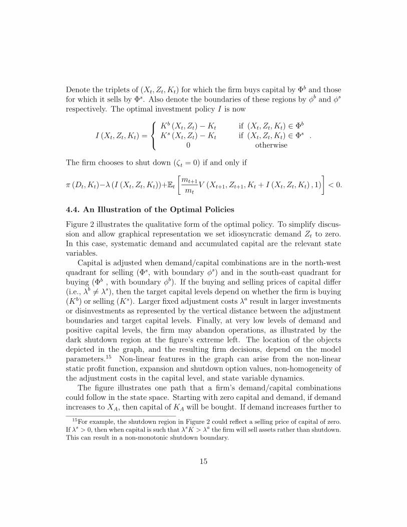
Denote the triplets of (Xt, Zt, Kt) for which the firm buys capital by Φb and thosefor which it sells by Φs. Also denote the boundaries of these regions by φb and φs

respectively. The optimal investment policy I is now

I (Xt, Zt, Kt) =

Kb (Xt, Zt)−Kt if (Xt, Zt, Kt) ∈ Φb

Ks (Xt, Zt)−Kt if (Xt, Zt, Kt) ∈ Φs

0 otherwise.

The firm chooses to shut down (ζt = 0) if and only if

π (Dt, Kt)−λ (I (Xt, Zt, Kt))+Et

[mt+1

mt

V (Xt+1, Zt+1, Kt + I (Xt, Zt, Kt) , 1)

]< 0.

4.4. An Illustration of the Optimal Policies

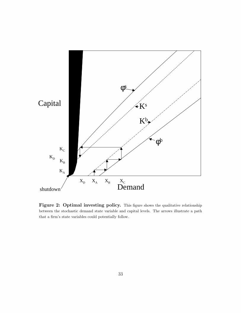
Figure 2 illustrates the qualitative form of the optimal policy. To simplify discus-sion and allow graphical representation we set idiosyncratic demand Zt to zero.In this case, systematic demand and accumulated capital are the relevant statevariables.

Capital is adjusted when demand/capital combinations are in the north-westquadrant for selling (Φs, with boundary φs) and in the south-east quadrant forbuying (Φb , with boundary φb). If the buying and selling prices of capital differ(i.e., λb 6= λs), then the target capital levels depend on whether the firm is buying(Kb) or selling (Ks). Larger fixed adjustment costs λa result in larger investmentsor disinvestments as represented by the vertical distance between the adjustmentboundaries and target capital levels. Finally, at very low levels of demand andpositive capital levels, the firm may abandon operations, as illustrated by thedark shutdown region at the figure’s extreme left. The location of the objectsdepicted in the graph, and the resulting firm decisions, depend on the modelparameters.15 Non-linear features in the graph can arise from the non-linearstatic profit function, expansion and shutdown option values, non-homogeneity ofthe adjustment costs in the capital level, and state variable dynamics.

The figure illustrates one path that a firm’s demand/capital combinationscould follow in the state space. Starting with zero capital and demand, if demandincreases to XA, then capital of KA will be bought. If demand increases further to

15For example, the shutdown region in Figure 2 could reflect a selling price of capital of zero.If λs > 0, then when capital is such that λsK > λa the firm will sell assets rather than shutdown.This can result in a non-monotonic shutdown boundary.

15

XB, a second expansion from KA to KB takes place. Further investment will beundertaken whenever the investing boundary is reached. Conversely, if demandfalls from XC , there will be no adjustment until demand falls to XD. At thatpoint physical plant is reduced from KC to KD as the firm sells capital.

5. Aggregate Economy Dynamics

Having solved the dynamic optimization problem of a single firm, we generatethe return dynamics of a cross-section of firms and estimate the model usingmoments of the data. The economy consists of a continuum of monopolistic firmsdistributed over the firm level state space. Each faces the demand dynamics setout in Sections 3 and 4. In particular, the demand for each monopolist’s productis affected by the common systematic component Xt. Indexing the firms by i, eachfirm has an independent and identically distributed idiosyncratic component totheir demand given by Zi

t . Each of the firms makes independent decisions aboutits optimal investment I i

t and hence the level of its capital stock Kit+1.

5.1. Entry

Our model incorporates exit through limited liability and shutdown. Since shut-down is irreversible, we must also permit entry or there would eventually be nofirms. We take a simple but economically intuitive approach, which is to assumethat entry opportunities are created by the exit of existing firms. We representfirms as infinitesimals, and while the mass of previously shutdown firms accumu-lates stochastically, the combined mass of active firms and potential entrants isheld constant. This assumption is appropriate for an economy with fixed invest-ment opportunities.

5.1.1. Potential Entrants

To formalize this approach, let

SE ≡ {Zt, Kt, Yt−1 : Zt ∈ X , Kt = 0, Yt−1 = 1}

be the partition of the firm-level state space reserved for new entrants. We notethat potential entrants are the only firms permitted to have zero capital.

Firms must belong to one of the three partitions corresponding to active in-cumbent states SA, previously shutdown states SD, and potential entrant states

16

SE. Let S∗ denote the union of these partitions, and for any s ⊆ S∗, let ψ∗t (s)denote the measure of firms in states belonging to s at date t.

Firms that abandoned operations prior to any date t are not relevant to thecross-section of future returns. Thus define S ≡ SA ∪ SE, and let ψt denote therestriction of the measure ψ∗t to S. Imposing that the measure of active firmsand potential entrants is constant over time, and for convenience normalizing thislevel to unity, we have ψt (S) = 1 for all t ≥ 0. The mass of potential entrants cannow be determined by the mass of active firms at the end of the previous period:

ψt

(SE)

= 1− ψt

(SA). (5.1)

Each potential entrant is given an independent draw for its idiosyncratic demandlevel Zi

t from the unconditional distribution of Z. Thus, for any idiosyncraticdemand level z, potential entrants are fully characterized by ψt (Zi

t = z, K it = 0) =

P (Z = z) ψt

(SE).

5.1.2. The Entry Decision

Each potential entrant has a single opportunity to begin operations. A firm thatdoes not enter is assigned the abandonment value of zero, and in the next perioda new potential entrant takes its place. There is thus no option value in waitingto enter. The model could be extended to accommodate this feature withoutdifficulty, but we seek to keep the entry decision as simple as possible since ourconcern in this paper is the cross-section of returns for publicly traded firms.

The firm enters with capital level Kb (Xt, Zit) if

Et

[mt+1

mt

V(Xt+1, Z

it+1, K

b(Xt, Z

it

))]− λbKb(Xt, Z

it

)− λa ≥ 0.

This requires that firm value upon entry exceed the cost of purchasing new capitalplus fixed adjustment costs.

5.2. Simulating the Cross-Section of Returns

Aggregate economy transition dynamics are now fully specified subject to initialconditions. The risks in the firm-level state variables Zi

t integrate out completelydue to our assumption that each firm is of infinitesimal size. The process {Xt} isthus the only exogenous state variable at the aggregate level. The distribution offirms ψt summarizes information relevant to the current and future cross-section

17

of returns that derives from the initial distribution ψ0 as well as the historyX0, ..., Xt−1 of demand. The aggregate state variables are thus Xt and the measureψt on the firm level state space S.

Assume initial conditions (X0, ψ0) where X0 ∈ X and ψ0 is a measure on Ssatisfying ψ0 (S) = 1. The dynamics of {Xt} are first-order Markov and the Ap-pendix shows that ψt+1 is fully determined by ψt and Xt, updated recursively. Bythen combining the time-series of firm cross-sections with numerically determinedexpected returns, calculated using the value function, portfolios can be formedand returns generated for any given set of model parameters.

6. Empirical Implementation

6.1. Methodology

We estimate the model using simulated method of moments, as in Ingram andLee (1991) and Duffie and Singleton (1993). Our estimator can also be viewed asa special case of indirect inference (Gourieroux, Monfort, and Renault, 1993). Anexcellent discussion of the these methods is in Gourieroux, Renault, and Touzi(2000).

The procedure is described in the Appendix, and we outline it here. Estimatesof a vector θ0 of true model parameters are desired. Given a candidate vector,data is simulated, and a set of moments are calculated. An objective function isused to compare these moments to those in the data, and the parameter vector isupdated to improve fit. The simulated method of moments estimator minimizesthe objective function.

In order to keep the estimation computationally tractable and to aid in iden-tification it is necessary to place a-priori restrictions on some parameters and toestimate others. In deciding which parameters to estimate we are guided by ourprimary motivation to understand how lumpy investment options, irreversibility,and operating leverage interact to generate return characteristics. Hence we es-timate the level f of fixed operating costs per unit capital, the fixed cost λa ofcapital adjustment, and the per-unit purchase price λb of capital. The optionto invest is also driven by the variance of both systematic and idiosyncratic de-mand shocks. We estimate σ2 ≡ σ2

z = σ2x to capture this effect in a parsimonious

manner. We also estimate the demand parameter b because it provides a role foroperating flexibility, which should affect operating leverage. Finally, we estimater and γ, which together determine risk premia.

18

The remaining parameters are fixed. The model roughly scales in costs and de-mands, and since we estimate several cost parameters, upper and lower boundariesfor X and Z are imposed exogenously.16 We also set the systematic proportion ofdemand to be α = 0.5. Finally, to capture the intuition that some irreversibility ininvestment is economically relevant, we fix λs = 0. We thus estimate a restrictedversion of the model with a vector

θ =[b, f, λa, λb, r, γ, σ2

]

of seven parameters.We use as moment conditions the mean return on decile portfolios of size-

sorted and book-to-market-sorted returns. The data is for the period July 1963through December 2001.17 Table 1 provides summary statistics for these returns.Following Cochrane (1996), we choose an identity weighting matrix.

Recalling the specific estimation strategy, for each potential set of parameters,optimal Markov investment policies under the model are calculated. We thensimulate ten independent time-series from the model under the optimal policies,each simulation with the same sample length as the data. Size and book-to-market decile portfolio excess return means are calculated and compared to thoseobserved in the real data. Given our choice of an identity weighting matrix, thecriterion being minimized is the sum of squared differences between the actual andsimulated expected excess returns from the size and book-to-market portfolios.

6.2. Results

Figure 3 shows that the model generates portfolios with mean excess returnssimilar to those in the data. The model captures considerable differences betweenthe unconditional returns of the extreme portfolios, with the return on the smallestsize portfolio 0.8% per month above the largest size portfolio. A similar fact is truefor the spread between the high and low book-to-market portfolios. Consistentwith the data, there is a monotonic relationship between expected return and size,and between expected return and book-to-market. The model even appears tomimic non-linearities in these relationships. Overall, the model approximates all20 portfolio mean returns well using just seven parameters.

The parameter estimates and their standard errors, reported in Table 2, pro-vide interesting insights. The operating cost parameter f is positive and signif-icant, and we therefore conclude that operating leverage is important. We also

16The appendix describes the lattice for these state variables.17This data was downloaded from the web site of Kenneth French.

19

conclude that a large purchase price of capital λb and demand volatility σ2 areessential. Returns are made less sensitive to demand shocks, in part, by the firm’sability to adjust instantaneous output. We speculate that high demand volatilityis also required to “mix” firms over time, leading to interesting aggregate dynam-ics for the portfolios. Adjustment costs λa are large, indicating that firms makeinfrequent lumpy investments. Finally, the stochastic discount factor parametersr and γ are large. This is not surprising, and shows that our model is consistentwith the equity premium puzzle.

Standard errors for the parameters provide a concrete metric by which togauge the relative importance of the various parameters in explaining the returnmoments. All of f , λb, r, γ, and σ2 are significant. On the other hand, the slopeof inverse demand b is not well identified. Interestingly, adjustment costs λa donot appear to be well-identified. This indicates that lumpy investment, resultingfrom high adjustment costs, is not critical for generating size and book-to-marketeffects.

The economic significance of the parameters can be assessed relative to thedemand shock distribution. We compare operating and capital costs to prices

and revenues at the 50th, 75th and 90th percentile demand levels. At the mediandemand level, a firm at the static optimal output level (K ≈ 4) has negative

operating profits. At the 75th and 90th percentile demand levels respectively,static optimum capital levels are about 9 and 14, fixed operating costs are 47% and32% of revenue, and the cost of one unit of capital is recovered after approximately36 and 20 months of operation. Regardless of the demand level, adjustment costsare roughly equal to the cost of a unit of capital. Because fixed operating andcapital costs are large at all but the highest demand levels, proper managementof growth options is essential to maximize firm value.

6.3. Comparative Statics

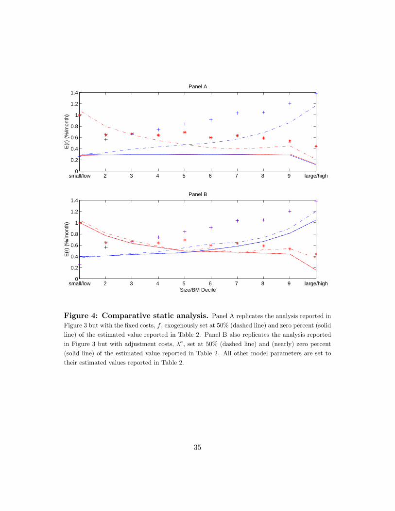
Figure 4 illustrates comparative static results at the optimal parameter estimates.Panel A demonstrates the effect of changes in fixed costs, f . The dashed lineillustrates the fit of the model when fixed costs are set at 50% of the value inTable 2. The solid line illustrates the fit of the model when these costs are set atzero percent. Panel B demonstrates the effect of changes in adjustment costs, λa.The dashed line illustrates the fit of the model when adjustment costs are set at50% of the value in Table 2. The solid line illustrates the fit of the model when

20

these costs are set at (nearly) zero percent.18

Consistent with the standard errors in Table 2, expected excess returns aresensitive to fixed operating costs but not fixed adjustment costs. Panel A showsthat when f = 0, expected excess returns are essentially constant, whereas inPanel B, wide variation in λa has little effect on expected returns. To understandthis result, recall that with lower adjustment costs target capital levels are closerto the adjustment boundaries (see Figure 2). It seems reasonable that size andbook-to-market effects would derive from regions of inactivity where capital levelsare not adjusted. Such regions can exist either because of fixed adjustment costsor irreversibilities. Thus, although lumpy investment may be required to explainother moments in the data (e.g., Cooper, 2003), it is not critical here. This resultis consistent with findings in Zhang (2003) and Xing (2003), who generate sizeand book-to-market effects without fixed adjustment costs. Our results indicatethat, in addition, operating leverage is critical for explaining the magnitude of thereturn characteristics.

6.4. Analysis of Higher Moments

Our model of firm behavior was designed to explain mean size and book-to-marketexcess returns, so these were an obvious choice to use in obtaining the simulatedmethod of moments estimates reported in Table 2. Other moments of returnsmight also be of interest, in particular variances and covariances. This subsec-tion investigates these higher moments, further verifying the intuition driving ourresults and providing other dimensions along which to evaluate the model.

Section 2 showed how size and book-to-market effects could result from lever-age associated with: (i) fixed operating costs that are tied to installed capital,or; (ii) growth options. Small firms or firms with high book-to-market have highexpected returns because of implicitly high leverage. The model should thereforealso imply high return volatilities and market index loadings for these firms.

To understand this intuition, note that our pricing kernel permits no time-series predictability. Thus, even though firm betas are time-varying, size andbook-to-market factors cannot arise. Portfolios with high unconditional meanreturns simply have high unconditional betas and variances. It would be veryinteresting, but beyond the scope of this paper, to endogenize the pricing kernelof our model and investigate whether size and book-to-market factors can result.

18For technical reasons, the numerical model requires strictly positive adjustment cost param-eters. Fixed costs, however, may be set to exactly zero.

21

Table 3 reports size and book-to-market portfolio standard deviations andbetas, from both the data and the simulations. The standard deviations of small-cap portfolios are high relative to large-cap portfolios in both the actual andsimulated data (top and bottom panels, respectively). In the simulated data,however, the absolute level of the standard deviations is much higher than in thedata. As noted previously, high variance in the demand state variable is requiredto generate expected returns that match the data. It is not surprising that thishigh variance is passed on to the portfolio returns.19 Unconditional betas are alsohigher for the “small” portfolios than for the “large” portfolios. In this case, themagnitudes of the simulated and actual betas are very close.20

For book-to-market sorted portfolios, the pattern of variances and covariancesobserved in the data is U-shaped. The “low” portfolio has a very high standarddeviation (7.59% per month) and beta (1.47). The standard deviation and betaof the “high” portfolio is also substantial. This pattern is not matched by thesimulated returns, where we see a monotonic relationship between the decile rankof the book-to-market portfolios and the standard deviations and betas.

To summarize, when using the estimated parameters from Table 2 the modelproduces size portfolio betas that are consistent with those found in the data.However, portfolio standard deviations are much too high. This result may berelated to our pricing kernel, which like many stochastic discount factors hasdifficulty addressing the equity premium puzzle. More difficult to explain arethe actual relationships among book-to-market portfolio standard deviations andbetas. The U-shaped pattern in these higher moments is not captured by ourcurrent specification. It is interesting to speculate what other sources of returnvariation might be useful to help reproduce these features of the data.

19Variance of demand is higher than variance of the returns because the production quantitydecisions of firms dampen the sensitivity of cash flows to demand shocks.

20Betas are calculated by regressing excess monthly portfolio returns on the excess monthlyindex return. In both the data and in the simulations, the equal-weighted market index wasused. (Similar results hold in the data with the value-weighted index, and the equal-weightedindex was chosen to match the portfolio returns generated in the simulations.) To accountfor the possibility of microstructure effects in the data, one lead and lag were added to theindex-model regressions and the reported beta is the sum of the coefficients on all three indexregressands.

22

7. Conclusion

We develop two models of the relation between expected returns and endogenouscorporate investment decisions. We obtain a new economic explanation for thebook-to-market effect as driven by operating leverage. When demand for a firm’sproduct decreases, equity value falls relative to book value, which is equal to thesize of the capital stock. With fixed operating costs that increase in the size ofthe capital stock, risk rises due to higher operating leverage. The models alsohighlight the importance of limits to growth in generating a size effect.

Our first model supposes a firm facing stochastic iso-elastic demand drivenby a lognormal diffusion. Firms have finite opportunities to irreversibly expandtheir capital base, and must pay fixed operating costs that vary with the level ofaccumulated capital. We derive closed-form expressions for expected returns, andshow that the firm beta is linear in the ratio of growth opportunities to assets inplace as well as the ratio of fixed costs to total firm value. We then show thatbook-to-market and size are sufficient statistics for operating leverage and theratio of growth opportunities to assets in place. We are thus able to relate sizeand book-to-market effects to sensible economic causes in a single factor modelwith closed form solutions.

The second model incorporates this basic intuition in a more realistic settingwith stationary dynamics. Our goal is to obtain a structural model that canbe estimated using standard methods. We suppose that a cross-sectional con-tinuum of monopolistic firms have demand dynamics composed of one commoncomponent, and for each firm a unique idiosyncratic component. The commonand idiosyncratic components are modeled as independent but statistically iden-tical stationary processes. We add realistic features including capital adjustmentcosts, costly reversibility of investment, limited liability and shutdown, and en-try. We find an optimal Markov strategy for each firm that is a function of thecommon and idiosyncratic demand components and the existing capital level ofthe firm. We estimate the model using the simulated method of moments. Asmoment conditions, we choose the mean excess returns on decile size and book-to-market portfolios. We find that the estimation method works well, and the modelaccounts both qualitatively and quantitatively for the size and book-to-marketeffects observed in the data.

23

8. Appendix

8.1. Proof of Proposition One

For any lifestage i = 0, 1, 2, denote V Ai (Xt) =

Qγi

δXt − fi

rfor the value of assets

in place and V Gi (Xt) = Vi (Xt) − V A

i (Xt) for growth options. When i = 1, thefirm can pay I2 to increase asset in place value from V A

1 (Xt) to V A2 (Xt). Given

exercise at x2 ≥ Xt, this option value is calculated as a perpetual binary optionwith payoff V A

2 (x2) − V A1 (x2) − I2. Let τ 2 (Xt) denote the random amount of

time that passes until x2 is reached. Discounting the payoff under the risk-neutralmeasure gives V G

1 (Xt) =[V A

2 (x2)− V A1 (x2)− I2

]Ee−rτ2(Xt). We then observe21

that Ee−rτ2(Xt) =(

Xt

x2

)ν

, where ν =√(

12− r−δ

σ2

)2+ 2r

σ2 + 12− r−δ

σ2 > 1, and the

inequality follows from δ > 0. To ensure that x2 is chosen optimally, the derivativeof V G

1 (Xt) with respect to x2 must be zero at all values of Xt. This gives theexpression for x2 in Proposition One, where ε2 = f2−f1+I2r

(ν−1)r. Substituting for x2 in

the formula for V G1 yields adolescent firm value. The value of the juvenile firm is

determined using similar arguments, where ε1 = f1−f0+I1r(ν−1)r

.

8.2. Proof of Proposition Two

Applying Ito’s lemma to the valuation equations from Proposition One yieldsdV =

[gXtVX + 1

2σ2X2

t VXX

]dt + σXtVXdBt. By inspection, an investment in

XtVX

Stunits of S instantaneously replicates firm value. Multiplying by S/V gives

the proportion of the replicating portfolio invested in S as VXXV

. Thus, firm betacan be derived directly from the elasticities of the valuation equations Vi(Xt) withrespect to X.

8.3. State Variable Dynamics

Both Xt and Zt take values in the set X = {x1, ..., xn}, which has elementsx1 = −0.6 and xn = 2.6 and xi+1 = xi + 0.2 for 1 ≤ i < n. The dynamics ofthe demand state variables X and Z are given by transition matrices Ax and Az

with elements axij = P (Xt+1 = xj |Xt = xi ) and az

ij = P (Zt+1 = xj |Zt = xi ). For

21See for example, Karlin and Taylor (1975), Section 7.5. For an alternative valuation ap-proach through the Bellman equation, see McDonald and Siegel (1986) or Dixit and Pindyck(1994), Section 5.2.

24

k ∈ {x, z}, let

akij =

σ2k/2 if j = i + 1pm

ki if j = iσ2

k/2 if j = i− 10 otherwise

.

The value pmki is 1− σ2 when 0 < i < n and adjusted at the boundaries i = 0, n to

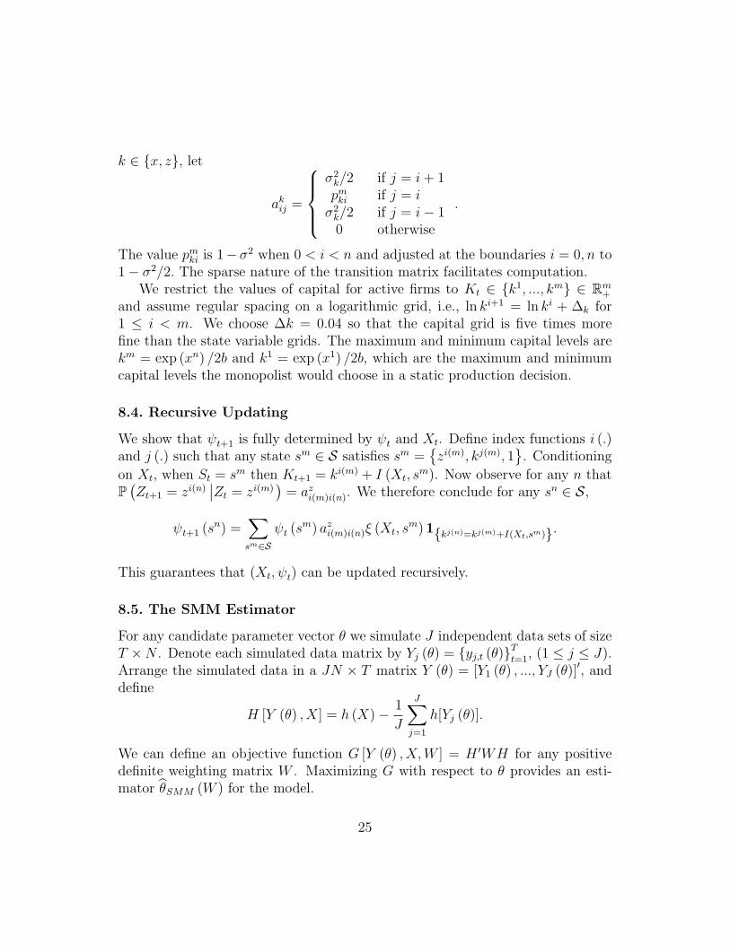
1− σ2/2. The sparse nature of the transition matrix facilitates computation.We restrict the values of capital for active firms to Kt ∈ {k1, ..., km} ∈ Rm

+

and assume regular spacing on a logarithmic grid, i.e., ln ki+1 = ln ki + ∆k for1 ≤ i < m. We choose ∆k = 0.04 so that the capital grid is five times morefine than the state variable grids. The maximum and minimum capital levels arekm = exp (xn) /2b and k1 = exp (x1) /2b, which are the maximum and minimumcapital levels the monopolist would choose in a static production decision.

8.4. Recursive Updating

We show that ψt+1 is fully determined by ψt and Xt. Define index functions i (.)and j (.) such that any state sm ∈ S satisfies sm =

{zi(m), kj(m), 1

}. Conditioning

on Xt, when St = sm then Kt+1 = ki(m) + I (Xt, sm). Now observe for any n that

P(Zt+1 = zi(n)

∣∣Zt = zi(m))

= azi(m)i(n). We therefore conclude for any sn ∈ S,

ψt+1 (sn) =∑sm∈S

ψt (sm) azi(m)i(n)ξ (Xt, s

m)1{kj(n)=kj(m)+I(Xt,sm)}.

This guarantees that (Xt, ψt) can be updated recursively.

8.5. The SMM Estimator

For any candidate parameter vector θ we simulate J independent data sets of sizeT ×N . Denote each simulated data matrix by Yj (θ) = {yj,t (θ)}T

t=1, (1 ≤ j ≤ J).Arrange the simulated data in a JN × T matrix Y (θ) = [Y1 (θ) , ..., YJ (θ)]′, anddefine

H [Y (θ) , X] = h (X)− 1

J

J∑j=1

h[Yj (θ)].

We can define an objective function G [Y (θ) , X, W ] = H ′WH for any positivedefinite weighting matrix W . Maximizing G with respect to θ provides an esti-mator θSMM (W ) for the model.

25

References

[1] Berk, J. (1995), A Critique of Size Related Anomalies, Review of FinancialStudies 8, 275-286.

[2] Berk, J., Green, R., and Naik, V. (1999), Optimal Investment, Growth Op-tions, and Security Returns, Journal of Finance 54, 1553-1607.

[3] Brennan, M. and Schwartz, E. (1985), Evaluating Natural Resource Invest-ments, Journal of Business 58, 135-157.

[4] Caballero, R. and Engel, E. (1999), Explaining Investment Dynamics in U.S.Manufacturing: A Generalized (S,s) Approach, Econometrica 67, 783-826.

[5] Clementi, G. (2003), IPOs and the Growth of Firms, Working paper,Carnegie Mellon University.

[6] Cooper, I. (2003), Asset Pricing Implications of Non-Convex AdjustmentCosts of Investment, Working Paper, Norwegian School of Management.

[7] Cochrane, J. (1996), A Cross-Sectional Test of an Investment-Based AssetPricing Model, Journal of Political Economy 104, 572-621.

[8] Daniel, K and Titman, S. (1997), Evidence on the Characteristics of CrossSectional Variation in Stock Returns, Journal of Finance 52, 572-621.

[9] Dixit, A., and Pindyck, R. (1994), Investment under Uncertainty, PrincetonUniversity Press, Princeton.

[10] Duffie, D., and Singleton, K. J. (1993), Simulated Moments Estimation ofMarkov Models of Asset Prices, Econometrica 61, 929-952.

[11] Ericson, R. and Pakes, A. (1995), Markov-Perfect Industry Dynamics: AFramework for Empirical Work, Review of Economic Studies 62, 53-82.

[12] Evans, D. (1987), The Relationship Between Firm Growth, Size, and Age:Estimates for 100 Manufacturing Industries, Journal of Industrial Economics35, 567-581.

[13] Fama, E. and French, K. (1992), The Cross-Section of Expected Stock Re-turns, Journal of Finance 47, 427-465.

26

[14] Fama, E. and French, K. (1993), Common Risk Factors in the Returns onStocks and Bonds, Journal of Financial Economics 33, 3-56.

[15] Ferson, W. and Harvey, C. (1999), Conditioning Variables and Cross-sectionof Stock Returns, Journal of Finance 54, 1325-1360.

[16] Gomes, J., Kogan, L., and Zhang, L. (2002), Equilibrium Cross-Section ofReturns, Journal of Political Economy, forthcoming.

[17] Gomes, J., and Livdan, D. (2002), Optimal Diversification: Reconciling The-ory and Evidence, Journal of Finance, forthcoming.

[18] Gourieroux, C., Monfort, A., and E. Renault (1993), Indirect Inference, Jour-nal of Applied Econometrics 8, S85-S118.

[19] Gourieroux, C., Renault, E., and Touzi, N. (2000), Calibration by Simulationfor Small Sample Bias Correction, in R. Mariano, T. Schuermann, and M.Weeks eds., Simulation-based Inference in Econometrics, Cambridge Univer-sity Press, Cambridge.

[20] Hall, B. (1987), The Relationship Between Firm Size and Firm Growth inthe US Manufacturing Sector, Journal of Industrial Economics 35, 583-606.

[21] Hansen, L., and Richard, S. (1987), The Role of Conditioning Information inDeducing Testable Restrictions Implied by Dynamic Asset Pricing Models,Econometrica 55, 587-613.

[22] Hopenhayn, H. (1992), Entry, Exit, and Firm Dynamics in Long Run Equi-librium, Econometrica 60, 1127-1150.

[23] Ingram, B. F., and Lee, B. S. (1991), Simulation Estimation of Time SeriesModels, Journal of Econometrics 47, 197-205.

[24] Johnson, T. C. (2002), Rational Momentum Effects, Journal of Finance 57,585-608.

[25] Karlin, S., and Taylor, H. (1975), A First Course in Stochastic Processes,Second Edition, Academic Press, San Diego.

[26] McDonald, R., and Siegel, D. (1985), Investment and the Valuation of Firmswhen there is an Option to Shut Down, International Economic Review 26,331-49.

27

[27] McDonald, R., and Siegel, D. (1986), The Value of Waiting to Invest, Quar-terly Journal of Economics 101, 707-727.

[28] Xing, Y. (2003), Firm Investments and Expected Equity Returns, WorkingPaper, Columbia University.

[29] Zhang, L. (2003), The Value Premium, Working Paper, University ofRochester.

28

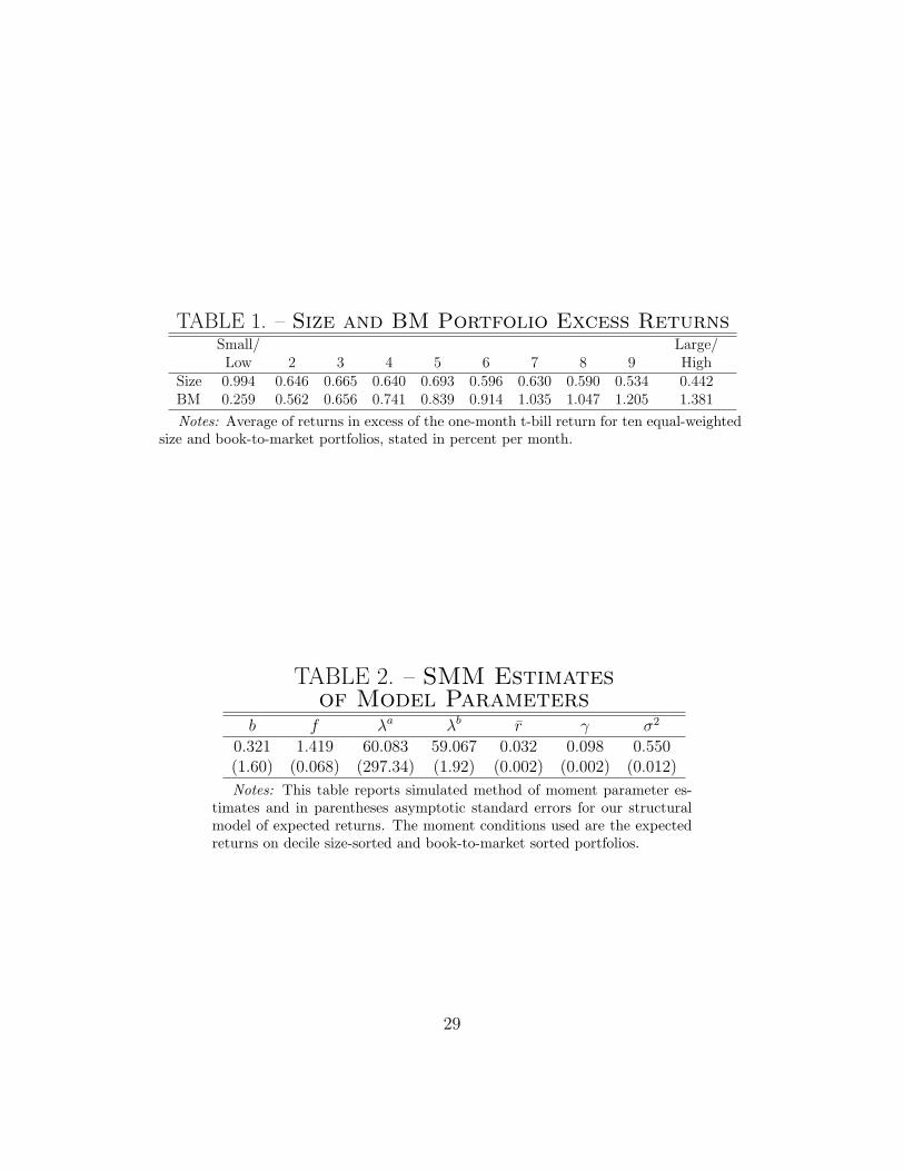
TABLE 1. – Size and BM Portfolio Excess ReturnsSmall/ Large/Low 2 3 4 5 6 7 8 9 High

Size 0.994 0.646 0.665 0.640 0.693 0.596 0.630 0.590 0.534 0.442BM 0.259 0.562 0.656 0.741 0.839 0.914 1.035 1.047 1.205 1.381

Notes: Average of returns in excess of the one-month t-bill return for ten equal-weightedsize and book-to-market portfolios, stated in percent per month.

TABLE 2. – SMM Estimatesof Model Parameters

b f λa λb r γ σ2

0.321 1.419 60.083 59.067 0.032 0.098 0.550(1.60) (0.068) (297.34) (1.92) (0.002) (0.002) (0.012)

Notes: This table reports simulated method of moment parameter es-timates and in parentheses asymptotic standard errors for our structuralmodel of expected returns. The moment conditions used are the expectedreturns on decile size-sorted and book-to-market sorted portfolios.

29

TABLE 3. – Higher Moments of Sizeand BM Excess Returns

Small/ Large/Low 2 3 4 5 6 7 8 9 High

Empirical MomentsSize s.d. 6.75 6.39 6.18 6.01 5.78 5.53 5.31 5.19 4.81 4.58

β 1.38 1.32 1.25 1.24 1.16 1.11 1.03 0.96 0.86 0.71

BM s.d. 7.59 6.39 6.05 5.76 5.45 5.31 5.18 5.25 5.54 6.30β 1.47 1.29 1.25 1.22 1.12 1.10 1.08 1.08 1.13 1.25

Simulated MomentsSize s.d. 37.35 28.58 24.35 21.74 19.79 19.26 17.83 17.03 16.78 17.33

β 1.72 1.32 1.12 0.99 0.90 0.85 0.80 0.77 0.75 0.77

BM s.d. 12.91 14.09 15.64 17.22 19.23 21.84 24.59 27.30 31.73 40.93β 0.59 0.65 0.71 0.78 0.86 0.96 1.08 1.22 1.45 1.87

Notes: Standard deviation (“s.d.”) and beta of excess returns for ten equal-weightedsize and book-to-market portfolios. Standard deviations are stated in percent per month.Betas are calculated relative to an equal-weighted market index using monthly data. Inorder to account for microstructure effects, betas reported in the top panel are the sum ofcoefficients in a regression which also includes one lead and lag of the excess index return.This correction is not applied to the simulated returns.

30

0 5 10 15 20 25 30 35 400

1000

2000

3000

4000A: Firm Value

Xt

V(X

t)

3 4 5 6 7 8 9 101

1.5

2

2.5

ln(Vit)

β t

B: Beta vs. Size

0 1 2 3 4 5 6 71

1.5

2

2.5

Book−to−Market

β t

C: Beta vs. Book−to−Market

x1 x

2

juvenile

adolescent

mature

mature adolescent

juvenile

juvenile

adolescent mature

Figure 1: Firm value, book-to-market and risk. This figure summarizes therelationship between demand and value (Panel A), size and risk (Panel B), and book-to-marketand risk (Panel C). When the demand state variable Xt is low, three types coexist: juveniles whohave not invested (solid line), adolescents who have invested once (dashed line), and mature firmswho have invested twice (dashed-dotted line). When demand reaches the critical level Xt = x1

31

for juvenile investment, value jumps discretely by the investment amount and valuation changesto that of an adolescent firm. Thus, in the region between x1 and x2 only two firm types exist.A similar change occurs when adolescent firms invest at Xt = x2 and become mature, so thatwhen Xt is high only mature firms exist. Panel B shows that firm size relates to firm beta.Each curve slopes downward, and the firm drops discretely to a lower curve when progressingto a new lifestage. Panel C shows that book-to-market is related to beta. The relationship ismonotonic for mature firms, and for reasonable portfolio weighting schemes low BM portfolioswill have lower expected returns than high BM portfolios. Model parameters are: r = .05,δ = .03, γ = 0.5, Q0 = 1, Q1 = 5, Q2 = 10, f0 = 1, f0 = 10, f2 = 20, λ1 = λ2 = 100, K0 = 100,K1 = 200 and K2 = 300.

32

shutdown

Capital

Demand

Kb

Ks

φs

φb

XA XB XCXD

KA

KB

KC

KD

Figure 2: Optimal investing policy. This figure shows the qualitative relationshipbetween the stochastic demand state variable and capital levels. The arrows illustrate a paththat a firm’s state variables could potentially follow.

33

small/low 2 3 4 5 6 7 8 9 large/high0.2

0.4

0.6

0.8

1

1.2

1.4

1.6

Size/BM Decile

E(r

) (%

/mon

th)

Size and BM Portfolio Returns

BM − Data

BM − Simulated

Size − Simulated

Size − Data

Figure 3: Size and book-to-market portfolio returns. This figure showsexpected returns to twenty portfolios formed based on size and book-to-market. The dashedand dashed-dotted lines summarize the returns in the data, based on the average monthlyreturn from 1963:07-2001:12. The solid lines represent the average returns from the model-based portfolios, using 10 simulations of length 300 months. Parameter values are those whichminimized the criterion function: b = 0.321, f = 1.419, λa = 60.083, λb = 59.067, r = 0.032,γ = 0.098 and σ2 = 0.550.

34

small/low 2 3 4 5 6 7 8 9 large/high0

0.2

0.4

0.6

0.8

1

1.2

1.4Panel B

Size/BM Decile

E(r

) (%

/mon

th)

small/low 2 3 4 5 6 7 8 9 large/high0

0.2

0.4

0.6

0.8

1

1.2

1.4Panel A

E(r

) (%

/mon

th)

Figure 4: Comparative static analysis. Panel A replicates the analysis reported inFigure 3 but with the fixed costs, f , exogenously set at 50% (dashed line) and zero percent (solidline) of the estimated value reported in Table 2. Panel B also replicates the analysis reportedin Figure 3 but with adjustment costs, λa, set at 50% (dashed line) and (nearly) zero percent(solid line) of the estimated value reported in Table 2. All other model parameters are set totheir estimated values reported in Table 2.

35