Corporate Governance and AggregateVolatility ∗

Thomas Philippon†

MIT

JOB MARKET PAPER

November 2002

AbstractThis paper argues that firms adapt their mode of governance to market conditions, andthat this may help us understand the business cycle. I focus on the extent of insiders’control over firm’s decisions. The delegation of control to insiders fosters initiative butit also gives them the opportunity to expand their firm beyond the profit-maximizingsize. This type of behavior has very different implications at the firm level and in theaggregate. At the firm level, it destroys value. In the aggregate, however, when goodsmarkets are imperfectly competitive, firms are too small relative to the social optimum.In such circumstances, insiders’ tendency to increase investment, employment and out-put are at once costly for shareholders and beneficial for the economy. Under plausibleassumptions, I show that firms find it optimal to delegate control when demand is high.A positive shock therefore induces more firms to delegate control. Because delegationitself increases output and productivity, the initial shock is amplified and other firmschoose to delegate control. I incorporate these insights into a standard real businesscycle model and show that delegation choices provide a powerful amplification mech-anism. Finally, the model predicts that an increase in firm volatility can decreaseaggregate volatility and I present evidence consistent with this prediction. (JEL D2,E3, E4, G3)

∗I am grateful to Olivier Blanchard and Ricardo Caballero for their insightful supervision, and to MariosAngeletos and Ivan Werning for their help and encouragement. I also benefited from the comments of DaronAcemoglu, Mark Gertler and Bengt Holmström. I thank Manuel Amador, David Bowman, John Faust,Francesco Franco, Augustin Landier, Gordon Phillips, John Reuter, Roberto Rigobon, Bernard Salanie andMichael Woodford, as well as seminar participants at the Federal Reserve Board, the IMF, MIT, Delta andCREST for their comments.

†Contact: philippo@mit.edu. Department of Economics, MIT, 50 Memorial Drive, Cambridge, MA 02142

1

1 Introduction

The question of who controls the firm is a central one in corporate finance. While the chain

of formal authority is fairly well defined (running from the investors to the board, from

the board to the CEO, and so on), effective control depends on how much of this formal

authority is retained and on how much of it is delegated. This paper argues that control is

tightened when business conditions deteriorate and that this has quantitatively important

implications for the business cycle.

The paper analyzes the following trade-off. Authority (i.e., the right to make discre-

tionary decisions) can be delegated to people inside firms. Delegation allows insiders to use

their specific skills and expertise, which enhances productivity. The cost of delegating con-

trol is that it creates room for opportunistic behavior. If one does not delegate and instead

asks people to go by the book, specific skills and expertise are partly lost, but so is egregious

misbehavior.

To go further, one needs to be more specific about the costs and benefits of delegation. I

follow Aghion and Tirole (1997) and Burkart, Gromb and Panunzi (1997) by assuming that

delegation fosters initiative and non-contractible investments. These investments translate

into higher productivity at the firm level. I model the costs of delegation as in Jensen (1986)

and Hart and Moore (1995), and argue that managers who enjoy discretionary control tend

to expand their firms beyond the profit-maximizing size.

The first insight of the paper is to notice that “empire building” behavior can have

very different implications at the firm level and in the aggregate. When goods markets are

imperfectly competitive, firms are too small relative to the social optimum. In this case,

managerial tendencies to increase investment, employment and output are at the same time

costly for shareholders and beneficial for the economy. On the other hand, other forms

of managerial misbehavior, such as stealing and spending on non-productive activities, are

socially wasteful.

Building on the idea that there is an important distinction between productive and non-

productive deviations from profit maximization, the paper proposes a simple model to study

the implications of firms’ governance choices for the business cycle. I assume that, at every

period, each firm must decide whether or not to delegate control to insiders. When control

is delegated, productivity is high but two distortions appear. First, output is too high.

Second, there is excess overhead labor. When control is not delegated, productivity is lower

2

but profit maximization can be strictly enforced. Because delegation increases productivity,

the benefits of delegation are higher the higher the demand for the firm’s product. On the

other hand, the costs of delegation do not increase one for one with the firm’s demand. It is

therefore optimal for the firms to delegate more when demand is high.

The main result of the paper is that these governance choices amplify aggregate fluctu-

ations. When a negative shock hits the economy, some firms switch to a more conservative

mode of governance because insiders’ initiatives become relatively less valuable than cost

cutting. This has three consequences, two of which amplify the initial shock: first, some

specific expertise is lost when control is tightened and this leads to a drop in productivity;

second, output goes back to the monopolistic level. The third consequence (less overhead

labor) dampens the negative shock by freeing resources that were previously misallocated.

The simulations below show that, at least for small initial deviations from profit maximiza-

tion, the first two effects dominate the third one. The net consequence is, therefore, an

amplification of the initial shock, which, in turn, leads other firms (suppliers or customers

of the downsizing firms, for instance) to tighten their governance strategy.

I consider two classes of aggregate shocks: technology shocks and labor supply shocks.

Governance choices amplify technology shocks by a factor of 1.5, and labor supply shocks

by a factor of 1.9. In the case of labor supply shocks, the model without the endogenous

governance mechanism predicts counter-cyclical real wages. The aggregate labor demand

schedule is fixed and therefore the wage has to fall in booms for firms to be willing to

hire more labor. This prediction is counter-factual. However, the governance model that I

calibrate predicts weakly procyclical real wages even when the business cycle is driven by

labor supply shocks. This is because a positive shock induces firms to delegate more control,

which makes them at the same time more productive and more willing to hire for a given

level of productivity. The aggregate demand for labor therefore shifts out and this increases

the equilibrium wage.

Finally, I use the model to propose a new explanation for the recent decline in aggregate

volatility. The amplification mechanism emphasized in this paper is based on the idea that

firms adapt their mode of governance to market conditions. But market conditions are

affected by both idiosyncratic and aggregate shocks. I document the fact that firm level

risk has increased over the past 40 years. This implies that the number of firms that would

change their behavior in response to any given macroeconomic shock is smaller nowadays

3

than it was in the past. As a consequence, the amplification mechanism is less powerful and

the economy is more stable. I calibrate the model using the actual increase in firm level

risk and I find that the model can predict 40% to 50% of the actual decrease in aggregate

volatility.

The paper is organized as follows. Section 2 discusses the related literature. Section 3

describes the economy. Section 4 discusses firms’ governance decisions. Section 5 presents

the intuition for the amplification mechanism. Section 6 discusses the empirical evidence

and describes the calibration method. Section 7 presents the impulse responses of the model

to technology and labor supply shocks. Section 8 compares the simulated economies with

actual data. Section 9 presents evidence on the increase in firm volatility over the past 40

years and computes the implied decrease in aggregate volatility for the calibrated model.

Section 10 concludes. Derivations and technical details are in the appendix.

2 Related Literature

This research is related to the microeconomic literature on governance conflicts between

managers and shareholders. Jensen (1986) emphasizes the idea that managers tend to expand

their firms beyond the profit-maximizing size. This “empire building” behavior also plays

a key role in Hart and Moore (1995). The idea that delegation fosters initiative and non-

contractible investments is presented in Aghion and Tirole (1997) and Burkart, Gromb and

Panunzi (1997). Scharfstein and Stein (2000) provide a model where preferences for large

firms arise endogenously from the interaction between two layers of agency. I will discuss

the empirical literature about governance conflicts in detail when I turn to the calibration

of the model.

The importance of imperfect competition for the business cycle has been emphasized by

Blanchard and Kiyotaki (1987), and Rotemberg and Woodford (1992) among others. The

empirical finding that markups of prices over marginal costs are counter-cyclical1 is relevant

for my paper because a firm operating on its demand curve can expand its output only by

lowering its markup. One expects to see lower markups when insiders control because they

put more weight on sales and employment relative to profits than outsiders do. Counter-

cyclical markups could then be driven by procyclical delegation of control to insiders.

Finally, this research is related to the literature that studies the macroeconomic impli-1See Rotemberg and Woodford (1999) for a survey, and Bils and Kahn (2000) for recent evidence.

4

cations of financial frictions: Bernanke, Gertler and Gilchrist (1999), Kiyotaki and Moore

(1997). The frictions that I emphasize are different in the sense that, in my model, firms do

not suffer from liquidity constraints.

3 Model

Consider an infinite horizon stochastic general equilibrium model. The consumers maximize

maxKt+1,Lt,Ct,ut

E0

"Xt

βtµlog (Ct)− 1

Zt

φ

φ+ 1L

φ+1φ

t

¶#(1)

subject to the budget constraint

(1 + g)Kt+1 = (1− δ (ut))Kt +WtLt + utRtKt +Πt − Ct − γ

2

(Kt+1 −Kt)2

Kt(2)

Rt is the rental price of capital services, ut is the rate of utilization of the existing stock of

capital Kt, Πt are aggregate profits, g is the trend growth rate of labor productivity and γ

captures adjustment costs for investment as in Hall (2002). Zt is an aggregate labor supply

shock2. The cost of higher utilization is captured by an increase in the depreciation rate

δ (ut) as in King and Rebelo (1999).

The economy produces a final good using differentiated inputs. The final good is produced

competitively and it can be used for consumption and investment. The differentiated goods

are produced by a continuum of mass N of firms indexed from 0 to 1. N will be determined

in equilibrium by a free entry condition. The production function for the final good is

Yt = N ×µZ 1

0

h1σity

σ−1σ

it

¶ σσ−1

(3)

and the final good producers solve

maxyitPtYt −N ×

Z 1

0

pityit

where yit is the production of intermediate good i at time t and hit is an exogenous firm

specific shock. The distribution of these shocks is time invariant and the mean is normalized

to one:R 10hit = 1. These shocks can be interpreted as relative productivity shocks from the

2Chari, Kehoe and McGrattan show how a model with nominal wage rigidities and monetary shocks canproduce such shocks. More generally, I am interested in non-technological disturbances, and the simplestway to introduce them is through shocks that affect households’ marginal rate of substitution betweenconsumption and leisure.

5

point of view of final good producers, or as relative demand shocks from the point of view

of intermediate goods producers.

Equation (3) implies that each producer i faces an isoelastic demand curve:

yit = hit × YtN×µpitPt

¶−σ(4)

The price level, Pt, is such thatR 10hit³pitPt

´1−σ= 1. This is also the zero profit condition

for the final good producers. There is monopolistic competition in the differentiated goods

sector. The production function for intermediate good i is characterized by constant returns

to variable factors and some fixed costs. The variable factors are the flow of capital services

kit and labor lit. The production function for good i at time t is:

yit = θt qit k1−αit lαit

θt is an aggregate technology shock and qit is the firm’s idiosyncratic productivity. The fixed

costs for firm i are Φ units of final good and an amount l∗it of overhead labor. The (real)

profits of firm i are therefore:

πit =pitPtyit −Wt (lit + l

∗it)−Rtkit − Φ

The simplest way to model the governance choice is to see it as a choice among two tech-

nologies. At every period, each firm i must choose to delegate control to its insiders of not.

I describe this choice with the dummy variable Dit ∈ {0, 1}. This choice is made after allthe shocks (Zt, θt, hit) have been observed.

The first mode of governance, which I will call the conservative mode, has no delegation

of control to insiders (Dit = 0). Productivity is low¡qit = q < 1

¢but there is no overhead

labor (l∗it = 0) and profit maximization is strictly enforced. Formally, when Dit = 0, the

program of the firm is

maxk,l

πit

subject to (4) and yit = θt q k1−αlα. The resulting profits are πit (0).

The second mode of governance, which I will call innovative, delegates control to the

insiders (Dit = 1). The innovative mode has a high productivity, qit = 1 > q, but it has two

distortions. First, there is excess overhead labor, l∗it = l∗ > 0, and, second, the objective

function of the firm is to maximize a weighted average of sales and profits. The weight the

6

insiders put on sales is η∗ ≥ 0. When Dit = 1, the program of the firm is

maxk,l

η∗ pityit + (1− η∗) πit

subject to (4) and yit = θt k1−αlα. The resulting profits are πit (1).

Finally, I assume that delegation is chosen to maximize the profits of firm i at time t.

Dit = arg maxD∈{0,1}

πit (D)

A rational expectations equilibrium for this economy is a set of stochastic processes for the

exogenous technology and labor supply shocks {θt, Zt} and for the endogenous prices andquantities. {Dit, lit, kit, pit}i solve the intermediate firms’ program described above, {Yt, yit}are determined by (3), and consumers maximize (1) over {Kt+1, Ct, Lt, ut, }. All the agentstake {Pt,Wt, Rt} as given, and the following market clearing conditions hold:

Yt = Ct + It +N × Φ

utKt = N ×Z 1

0

kitdi

Lt = N ×Z 1

0

(lit +Dit × l∗) di

This definition of equilibrium is conditional on the number of firms, N , which is constant.

To pin down N , I impose that a free entry condition holds in the non-stochastic steady state

of the economy (see Rotemberg and Woodford, 1999 and the appendix).

4 Governance Choice

There are many ways to motivate the reduced form used above and a formal model is pre-

sented in the appendix. Before discussing the interpretation of the reduced form, I describe

how firms choose among the two modes of governance.

Assumption 1: κ (η∗) > qσ−1 where κ (η) ≡ 1−σ η(1−η)σ

Assumption 1 ensures that delegation is sometimes desirable. The function κ is concave

and reaches a maximum of one for η = 0. It reflects the profit losses coming from the fact that

firms in the innovative mode deviate from the objective of profit maximization. For given

factor prices (W and R), and demand conditions (h and Y ), the cash flows generated by firm

i (before overhead costs are paid) are proportional to κ (η)× qσ−1. In the innovative mode,

7

this becomes κ (η∗)× 1 and in the conservative mode, 1× qσ−1. Assumption 1 ensures thatthe gains from innovative efforts outweigh the losses from excessive production. Proposition

1 describes the optimal governance choice for firm i at time t.

Proposition 1 Firm i will choose the innovative mode of governance at time t if and only

if

hit > h∗t

where

h∗t =Wt

At

l∗

κ (η∗)− qσ−1 (5)

At ≡õ

θt

µRt1− α

¶1−αµWt

α

¶α!1−σ

YtσN

Proof. In the innovative mode of governance, the choice of production is made to

maximize η∗pityit + (1− η∗)πit. The resulting profits are π∗it = At hit κ∗ −Wt l

∗, where κ∗ is

defined in assumption 1 and l∗ is excess overhead labor. In the conservative mode, profits

are simply πit = At hit qσ−1. Comparing the two levels of profits completes the proof.

The economic intuition is fairly straightforward. Because delegation increases initiative,

delegation is more valuable when the demand for the firm’s product is high. On the other

hand, the costs of delegation do not increase one for one with the firm’s demand. Thus, the

choice of governance mode takes the form of a simple cutoff rule: firms that do well (high h)

choose the innovative mode and firms that do poorly (low h) choose the conservative mode.

The cutoff h∗t depends on the overhead labor distortion and on the aggregate conditions in

the economy. It is relatively more costly to delegate when the real wage is high, because

of overhead labor costs. The effects of aggregate demand, Yt, and of the marginal cost of

production, 1θt

¡Rt1−α¢1−α ¡Wt

α

¢α, are standard. As Yt increases, delegation becomes relatively

more valuable, and the opposite happens for an increase in the rental price or in the real

wage (independently of the overhead labor cost).

The assumption that some of the delegation costs become relatively smaller when the

firm does well is crucial for the result that delegation is more valuable in a boom. I will

argue below that this is an empirically plausible assumption. Furthermore, the model by

Scharfstein and Stein (2001) has this implication.

8

I can now discuss two interpretations of the model. The first one follows closely Burkart,

Gromb and Panunzi (1997) and Aghion and Tirole (1997). In their model, a principal

chooses to delegate more or less control to an agent. There are many such relationships

inside firms, but, for concreteness, one can think of the principal as the board of directors

and the agent as the CEO. The board can decide how much it wants to interfere with the

CEO’s decisions. Freedom fosters productive initiatives (q = 1) but the CEO then has some

discretion concerning the corporate objective. In particular, she has a preference for large

firms (η∗ > 0) and for overhead labor (l∗ > 0). The two key assumptions in this setup are

that the CEO has some empire building tendencies, and that selective intervention is not

an option. More precisely, delegation can improve CEO’s incentives to make firm-specific

investments precisely because delegation is a commitment not to intervene ex-post. In this

case, the “innovative” governance mode can be seen as a solution to the hold-up problem.

The second interpretation follows Scharfstein and Stein (2000). Two features of their

model are particularly relevant for my approach. First, Scharfstein and Stein show that

preferences for large firms can arise endogenously in a setup with two layers of agencies,

one between the board and the CEO, and a second one between the CEO and the division

managers. In their model, because the CEO is an agent, she may decide to compensate the

division managers with a distorted production structure instead of using monetary transfers.

The second interesting feature of their model is that the inefficiencies arise from rent-seeking

activities that take time away from productive work. Since the opportunity cost of these

activities is high when the demand for the firm’s product is high, their model predicts that

some of the agency costs do not increase one for one with the firm’s demand. The overhead

labor cost (l∗) captures this idea in a crude way: it is a fixed cost of delegation.

It may be useful to emphasize that the kind of delegation mechanism I have just described

can be implemented with a non-contingent debt contract. Indeed, there is a monotonic

relationship between firm’s profits and the extent of insiders’ control. One can therefore

think of the governance decision as a contract that says that insiders get to keep discretionary

control over the firm’s operations as long as cash flows exceed some threshold. This is close to

the interpretation the “control right” literature gives of a debt contract (Aghion and Bolton,

1992, Hart 2001).

In the calibration below, the distortions will be small. In particular, the baseline model

uses parameter values such that the drop in productivity¡1− q¢ when control is tightened is

9

1% and the total losses from all governance issues (productivity, excess production and excess

overhead labor) are less than 3% of firm value. Discretionary overhead labor represents less

than 1% of total employment.

5 Amplification

The main result of the paper is that firms’ delegation choices amplify aggregate shocks.

Before turning to the simulations of the model, it is useful to present the intuition for this

result. From the definition of the aggregate price level and from the pricing decisions of the

intermediate goods producers, one can obtain the following equation

µ× ct ="J (h∗t )×

µ1

1− η∗

¶σ−1+ (1− J (h∗t ))× qσ−1

# 1σ−1

(6)

where

ct =1

θt

µRt1− α

¶1−αµWt

α

¶α

is the marginal cost associated with the Cobb-Douglas production function. J (h∗t ) =R∞h∗th f (h) dh and f (.) is the distribution function of the idiosyncratic shocks h. Equation

(6) is shared by all general equilibrium models of imperfect competition where the pricing

behavior of firms is described by pitPt= µit × cit. Most models focus on the symmetric equi-

librium where all firms have the same marginal cost cit = ct and the same markup µit = µ.

In a symmetric equilibrium, one would get the simple condition: µ × ct = 1. In my modelhowever, firms differ in both their marginal costs and their markups. Firms that choose to

delegate control have higher productivity qit = 1 and lower markups µit = (1− η∗)×µ thanother firms. Equation (6) can be seen either as defining the aggregate markup as a weighted

average of the firms’ markups or as defining the aggregate marginal cost as a weighted aver-

age of the firms’ marginal costs. The weight on the innovative firms is J (h∗t ). Because the

markup choices are correlated with firms’ idiosyncratic productivity, one cannot in general

disentangle the aggregate markup from the aggregate marginal cost. But one can consider

a few special cases.

• l∗ = 0. In this case, we know from proposition 1 that h∗t = 0. Since J (0) = 1, we get

(1− η∗)µ× c = 1. In this symmetric equilibrium, all firms charge the same price butthey deviate from the profit maximizing markup µ by a factor 1− η∗.

10

• η∗ = 0. In this case, all firms charge the profit maximizing markup but productivity

levels differ across firms. This case is isomorphic to a model with increasing returns at

the firm level. To see why, interpret Wtl∗t not as a cost of delegation due to managerial

misbehavior, but as a fixed cost of operating a high productivity technology. Firms

choose this technology only when they face a high demand. The aggregate marginal

cost decreases when the weight of high productivity firms increases.

Using the definition of the cutoff (5) together with equation (6), I get

h∗t

J (h∗t )׳

11−η∗

´σ−1+ (1− J (h∗t ))× qσ−1

=Wt

Yt

σNl∗

κ (η∗)− qσ−1

In this equation, the LHS is increasing in h∗t . The RHS increases withW and decreases with

Y . We can now understand the amplification mechanism. Consider the case of a positive

technology shock. Following the shock, output will increase but so will the real wage. If

factor supplies are elastic, output will increase more than the real wage and this will push

the cutoff h∗t to the left and lead some firms to switch to the innovative mode of governance.

These firms will then hire more capital and labor and increase their output. Again, if

factor supplies are elastic, this will increase output more than it will increase the wage and

h∗t will move further to the left3. We therefore expect the amplification mechanism to be

stronger when factor supplies are elastic. This is why the presence of capacity utilization is

important in this model. It is well understood that capacity utilization makes the standard

RBC model more responsive to shocks (King and Rebelo 1999). Here, this will also apply

to the amplification factor over and above what the RBC would predict.

6 Calibration

I will now describe briefly the calibration procedure. All data are detrended using the HP

filter. I consider the impact of labor market disturbances, captured by the parameter Zt and

aggregate technology shocks θt.

There are three non-standard parameters in the model described above: η∗, l∗ and q.

A key feature is that these parameters will have different effects on profits, sales and em-

ployment, respectively. η∗ captures over-expansion. It increases sales and employment and3This suggests that the model could have multiple equilibria. This is indeed a possibility. For the

parameter values that I estimate however, idiosyncratic risk is high enough to remove this possibility.

11

decreases profits. l∗ captures non-productive expenses. It has no impact on sales and em-

ployment, and a negative impact on profits. Finally, productive initiatives q are going to

increase sales, profits and employment. The following table summarizes the predictions.

Effect of parameters on: Profits Sales Employmentη∗ - + +l∗ - 0 0q + + +

Berger and Ofek (1999) show that the amount of unallocated expenses is a strong deter-

minant of corporate refocusing programs. Lichtenberg and Siegel (1990) focus on ownership

changes and show that employment growth is much lower in establishments changing owners

than in those not changing owners, and that the effect is stronger for auxiliary establishments

than for production establishments. This is consistent with my assumption that l∗ is strictly

positive. Berger and Ofek (1999) also show that disciplinary events (shareholder pressure,

financial distress, management turnover) usually occur before refocusing takes place and are

followed by average cumulative abnormal returns of 7%. Denis and Kruse (2000) show that

the corporate restructuring following declines in performance involves major cost cutting

efforts, plant closing, asset sales and layoffs. These restructuring efforts increase shareholder

value (see also Gilson, 1998). Denis and Denis (1995) show that, following a normal re-

tirement of the CEO at age 65, the median firm experiences an employment decline of 7%,

suggesting that the firm was previously too fat. Similarly, Kaplan (1989) finds that MBOs

are followed by declines in employment, sales and investment, and by increases in profits.

These results suggest that both η∗ and l∗ are positive. Suppose that a firm has η = 3%

and that the elasticity of substitution between goods is σ = 4. Then a disciplinary event that

brings η down to 0 will be associated with a drop in sales and employment of 9% because

sales and employment are proportional to (1− η)1−σ. But note that this will have very

little impact on the firm’s profits since κ (3%) ≈ 1 by the envelope theorem. This suggeststhat l∗ > 0 is needed to explain significant effects on profits without unrealistically large

changes in sales. Indeed, a simultaneous decline in η∗ and l∗ can simply be interpreted as

a firm that downsizes its activities by closing its less productive plants first. To see why,

suppose that the firm has two plants with fixed capacity and fixed productivity. Profits

would be maximized by closing the less productive plant but the manager is reluctant to do

so. When a bad shock hits the firm, the manager is forced to close the plant. Profits go up

and production goes down.

12

One can also obtain evidence from the literature that studies the effects of leverage on

firms’ behavior. As I have explained above, one can think of implementing the delegation

mechanism with a debt contract. Empirically, one sees that more highly leveraged firms

charge higher prices and respond more quickly and more strongly to shocks: Phillips (1995),

Sharpe (1994), Chevalier and Scharfstein (1996). Kovenock and Phillips (1997) confirm the

results in Kaplan (1989) that LBO firms decrease their investment and show that this effect

is stronger in highly concentrated industries. Opler and Titman (1994) show that firms in

financial distress experience large drops in sales and employment beyond what one would

expect from the direct effects of the shock. The distressed firms lose market shares to their

competitors. The idea that leverage can be used to put pressure on insiders is also directly

supported by the fact that boards increase the leverage of their companies in response to

an increase in unions’ power (Gary Gorton and Frank Schmid (2000) for Germany, Stephen

Bronars and Donald Deere (1991) for the US). Finally, it is important to emphasize that

debt contracts are almost never contingent on aggregate shocks. Since corporate profits are

strongly procyclical, this means that effective debt constraints are counter-cyclical and this

provides support for the idea that insiders enjoy more freedom in booms than in recessions.

First, I choose h∗ such that, in steady state, half of the firms are in the conservative

governance mode and half of the firms are in the innovative mode. Based on the empirical

evidence discussed above, I set η∗ = 3% and 1 − q = 1%. I use σ = 4 as a benchmark

for the elasticity of substitution between goods. This implies a value-added markup of 1.33

consistent with Rotemberg and Woodford (1999). These values for η∗ and σ imply that for

half of the firms, sales are 9% higher than they would be under strict profit maximization

(holding productivity constant). The profit losses from this deviation are very small (1−κ∗ =0.6%). The value of q implies that the penalty for downsizing is a temporary productivity

loss of one percent.

The adjustment cost parameter γ is set to 4 (at quarterly frequency), following Hall

(2002). The elasticity of depreciation with respect to utilization is 0.2 consistent with King

and Rebelo (1999). The labor supply elasticity φ is 4 as in the benchmark RBC model (see

for instance King and Rebelo 1999).

µ φ η∗ q φ γ δ”(1)δ0(1)

1.33 4 3% .99 4 4 0.2

The steady state is computed to match the standard ratios ( CGDP

, WLGDP

, KGDP

). Recall

13

that free entry drives the profits to 0 on the balanced growth path. This pins down N and

Φ. The implied value for l∗ is such that the average excess overhead labor is less than 1%

of the employed population. The total ex-ante losses from all governance conflicts combined

are 2.27%

E [l∗]L

= 0.82%

E [π|q = 1, l∗ = 0, η∗ = 0] +RKN

E [π] +RKN

− 1 = 2.27%

Finally, the distribution of idiosyncratic shocks (h) is such that the 4-quarters standard

deviation of the growth rate of sales across firms is 12%, which is the empirical value in the

first half of the sample period4 (see below).

The model can then be log-linearized around its balanced growth path. I describe here

the calibration with the labor supply shock. log (Zt) is specified as an AR(1) process:

zt = ρzt−1 + εt

The model has one state variable (capital stock) and one exogenous driving process (z).

Note however that z is not observable in the data and that ρ is not known. The calibration

procedure follows the strategy used by King and Rebelo 1999. I make an initial guess for ρ.

Given this guess, I solve the model using rational expectations. The solution takes the form

byt = βyk × bkt + βyz × bztThe coefficient βyk and βyz are complex functions of all the parameters of the model and of

ρ. This equation for output can be inverted into bzt = 1βyz× byt− βyk

βyz×bkt. Using actual values

for byt and bkt, one can create a series for bzt. One can then compute the AR(1) coefficient forthis series. It is, in general, different from the original ρ. This value is then used as a new

starting point. The procedure is repeated until convergence. The estimated value of ρ is .89

(I estimated essentially the same values for z and for θ).

7 Impulse Responses

The intuition for the amplification mechanism is the following. Firms that have a low

demand hit < h∗t are in the conservative governance mode: they have no overhead labor, low4This is assuming that the h shocks are iid at the annual frequency. I have also experimented with an

AR(1) process for h. The results were quantitatively similar.

14

productivity and high markup. Following a positive aggregate shock, output Yt and factor

prices Rt and Wt are going to increase. To the extent that the labor supply is elastic and

that capacity utilization can accommodate the increase in the demand for capital services,

the rise in factor prices will not undo the initial rise in output and h∗t will decrease. Some

firms will therefore switch to the innovative mode of governance. They will reduce their

markups, increase their productivity but also hire excess overhead labor. The net effect of

these actions for the economy is positive and this leads other firms to follow the same path.

7.1 Technology Shocks

Figure 1 shows the response of the model to a positive technology shock. The shock is the

dotted line. GDP is the solid line. The third line represents the fraction of firms that choose

the conservative mode compared to the steady state value of 50%. Over time, the economy

accumulates capital and the initial shock fades away. This drives up the wage relative to

output, making it more costly for firms to have excess overhead labor. As h∗t increases, some

firms tighten control and output is pushed below its steady state value.

Figure 2 shows the impulse responses of different models to a positive technology shock

(θ). The exogenous shock (θ) is the same as in figure 1. The dotted line is the textbook

RBC. Above is the RBC with capacity utilization and adjustment costs for investment. This

model provides much stronger amplification than the basic RBC. The dashed line is the

governance model with only the productivity channel, q < 1 and η∗ = 0. In this model,

firms that switch from conservative to innovative governance are more productive but they

have excess overhead labor. As explained in section 5, this case can be interpreted as an

economy with some increasing returns at the firm level. This flattens the aggregate marginal

cost curve and creates amplification. The solid line is the model with q < 1 and η∗ > 0. In

this model, the innovative firms are not only more productive, but they also expand output

beyond the profit-maximizing size. This second channel of amplification works like in other

models of counter-cyclical markups (Rotemberg and Woodford, 1999).

7.2 Labor Supply Shocks

Figure 3 shows the impulse response of the model with respect to aggregate labor supply

shocks, Zt. The results are similar to the ones obtained with technology shocks but the

amplification compared to the augmented RBC model (with capacity utilization and adjust-

15

ment costs) is larger. This is because a positive labor supply shock will, all other things

equal, tend to decrease the real wage. This decreases the costs of excess overhead labor and

makes delegation more attractive.

Figure 4 compares the impulse responses of GDP to a positive labor supply shock for

different models. The governance model delivers strong amplification by two channels, pro-

ductivity and markup. The model with only the productivity effect delivers substantially

less amplification. Finally, as in the case of technology shocks, we see that capital utilization

plays an important role.

8 Simulations

I now turn to the comparison of the simulated models with actual US data.

8.1 Technology Shocks

Figure 5 shows the governance amplification in the model driven by technology shocks.

Amplification can be seen in two ways. In the top panel, the governance model is calibrated

to fit the GDP series (the solid line). Then the structural technology shocks (θ) from this

model are put into the augmented RBC model and into the standard RBC model. The

figure shows that output would have been less volatile without the governance mechanism.

The amplification is 1.5 compared to the augmented RBC and 3 compared to the textbook

RBC.

In the bottom panel, the same result is shown in a different way. This time, both the

RBC and the governance model are independently calibrated. The figure shows the path of

the technological driving process θ implied by the two models. The shock implied by the

augmented RBC is one and a half times more volatile than the one implied by the governance

model.

8.2 Labor Shocks

Figure 6 shows the overall fit of the governance model driven by labor shocks. There is

nothing impressive about the way the model fits the GDP series. This is a mechanical

consequence of the calibration procedure. The model should only be judged based on how

well it fits the other series.

16

Figure 7 shows the governance mechanism at work. In a boom, more firms are in the

innovative mode and aggregate productivity is higher. The bottom panel shows that the

model is able to replicate the behavior of the (uncorrected) Solow residual. In fact, this is

entirely due to the presence of fixed costs and capacity utilization. The correct technological

residual (defined over gross output and controlling for utilization) looks nearly constant

compared to the Solow residual. In other words, a model without endogenous governance

but with the same average markup would also fit the Solow residual. However, the model

without governance conflicts would need much larger labor shocks and would make counter-

factual predictions concerning the behavior of the real wage, as one can see on the next two

figures.

Figure 8 shows the labor shocks implied by the different models. The governance mech-

anism provides an amplification of 1.9 compared to either the RBC model or the imperfect

competition model with exogenous markups and productivity.

Figure 9 shows that the models without endogenous governance predict a counter-cyclical

real wage. The governance model reverses this prediction. This is a well known result from

the literature on counter-cyclical markups (see Rotemberg and Woodford, 1999).

9 The rise in idiosyncratic risk and the fall in aggregatevolatility

The decline is aggregate volatility was first described by Kim and Nelson (1999) and Mc-

Connell and Perez-Quiros (2000). Both papers conclude that the decline happened in the

first quarter of 1984. Blanchard and Simon (2000) interpret the same finding as evidence of

a downward trend in the post-war period, interrupted by a period of high instability in the

1970s. Stock andWatson (2002) present a very detailed study of the phenomenon. They pro-

vide new evidence on the quantitative importance of various explanations for the increased

stability of the economy and reach mixed conclusions: “Taken together, we estimate that

the moderation in volatility is attributable to a combination of improved policy (20-30%),

identifiable good luck in the form of productivity and commodity price shocks (20-30%), and

other unknown forms of good luck that manifest themselves as smaller reduced form forecast

errors (40-60%).”

I will now propose a tentative explanation for the “unknown forms of good luck.” First,

I will document the fact that the decrease in aggregate volatility coincided with a large

17

increase in firm level volatility. Second, I will show that the model presented above can

rationalize the two facts, and that it suggests a unified explanation.

Campbell, Lettau, Malkiel and Xu (2001) show that individual stocks have become more

volatile. The increase is very large: individual stocks volatility was multiplied by more

than two between the 1960s and the 1990s. My first task is to document the same fact

using “real” (as opposed to financial) data on employment and sales. Chaney, Gabaix and

Philippon (2002) look at firm level data using COMPUSTAT. Define the growth rate of the

sales of company i between time t and time t+ 1:

sit =

pit+1Pt+1

yit+1 − pitPtyit

pitPtyit

Let Nt be the number of companies in the sample at time t, and define firm level volatility

at time t as: eσ2t = Pi s2it

Nt−µP

i sitNt

¶2If one does this exercise on the full sample, one sees an enormous increase from 1960 to 2001

(figure 10). But, of course, there is entry in the panel and entrants are smaller and more

volatile (there are many more “small” firms in COMPUSTAT in 2001 than there were in

1960). The results also hold controlling for firm size (in real terms), but this is only half

convincing since, with technological progress, the same real sales in 2001 represent a smaller

firm than in 1960. So I also computed the volatility using only firms with more than 1000

employees. The trend is still very large in this sub-sample (figure 11). A simple way to

summarize the results is to compute the size weighted standard deviation, which is similar

to what Campbell et. al. did for stock prices. Let ωit be the weight of firm i at time t :

ωit =pityitPj pjtyjt

Define the average sales growth as

st =Xi

ωitsit

and define the size weighted volatility as

σ2t =Xi

ωit (sit − st)2

The size weighted volatility is the answer to the following question: suppose you pick at

random a “chunk” of sales in the sample; what would its volatility be? The results of this

18

exercise are shown on figure 125. The aggregate GDP volatility is computed using a 15

quarters rolling window. The two series have been scaled to fit on the same figure. Size

weighted firm level volatility is 12% on average before 1984, and it is 20% on average after

1984.6

The governance model suggests a mechanism through which an increase in firm level

volatility can lead to a decrease in aggregate volatility. In fact, the model suggests two such

mechanisms.

The first and most straightforward mechanism is an increase in the standard deviation

of the h distribution. This will mechanically increase firm level risk. It will also decrease

aggregate volatility. The reason is that firms in the tails of the distribution do not change

their governance after an aggregate shock. Firms with very low h are conservative in booms,

and firms with high h are innovative in recessions. As I have explained above, the aggregate

multiplier is a function of how many firms switch for a given aggregate shock. This fraction is

smaller when the distribution of the h shocks is more spread out. This leads to less aggregate

volatility. I will go a step further and ask what decline in aggregate risk the model predicts

based on the actual increase in firm level risk. The model was calibrated using a value for

firm level risk of 12%, which corresponds to the pre-1984 period7. I will therefore increase

the volatility of h by exactly the amount required to create a theoretical volatility of 20%

(the post-1984 average), keeping all other parameters constant. The results are summarized

in the following table. The actual decline is from 2.71 to 1.5%. The model predicts a decline

from 2.74 to 2.1%

2 Periods are: 1964:84, 84:2001. Standard Deviation of Cyclical GDP (HP filtered)Actual Change in Volatility 2.71 down to 1.5%Implied by increase in h− shocks 2.74 down to 2.1%

The second mechanism attempts to explain both fact by an increase in σ, or equivalently,

a decrease in the average markup. The increase in σ leads to more competition in the goods

market. This will amplify the effects of the firm specific shocks, q and η, and lead to an

increase in firm level volatility. On the macroeconomic front, a decrease in the average5I removed outliers by truncating at the 4th and 96th percentiles of the distribution of growth rates.6There are still many issues with these data. Perhaps most important is the issue of Mergers and

Acquisitions. We try to correct for these biases in Chaney, Gabaix and Philippon (2002), but the mostconvincing evidence against a purely M&A driven phenomenon is that Campbell et. al. document the samefact using daily stock returns.

7And a log-normal distribution for h.

19

markup also implies a less volatile markup. This will stabilize the economy. The results are

summarized in the following table.

2 Periods are: 1964:84, 84:2001. Aggregate Volatility Firm VolatilityActual Changes 2.71 down to 1.5% 12 up to 20%Implied by increase of σ from 4 to 7 2.74 down to 2.2% 12 up to 20%

Finally, the last figure shows how the implied labor shocks change once one controls for

the increase in firm level volatility. The top panel is the calibrated innovation of the process

for the labor supply shock using the benchmark model. The bottom panel shows the same

series for the pre-1984 period and shows the innovations calibrated using the economy with

large idiosyncratic risk for the post-1984 period. On the top panel, one can clearly see the

decrease in volatility starting in 1984. On the bottom panel, the “break” in volatility is

much less obvious. In other words, some of the decline in aggregate volatility would have

happened even without the decline in the volatility of the “structural” shocks, simply because

the economy is now more stable.

10 Conclusion

The main goal of this paper was to study the macroeconomic consequences of the governance

conflicts that have been emphasized in the corporate finance literature. I have shown that

these conflicts amplify aggregate fluctuations via two channels. First, one can see the delega-

tion of control to insiders as a technology that yields high productivity but also involves some

fixed costs. This makes it similar to an increasing returns technology. The fact that more

firms opt for this technology when demand is high flattens the aggregate marginal cost curve

and makes the economy more responsive to shocks. The second channel of amplification is

similar to the one found in models of counter-cyclical markups. A firm’s size moves closer

to the social optimum when insiders control because insiders increase output beyond the

level that a monopolist would choose. In a reduced form, procyclical insiders’ control yields

counter-cyclical markups. The calibrated model implies that these two channels create an

amplification factor of 1.5 for technology shocks and 1.9 for labor supply shocks.

The model also led me to consider a new explanation for the recent decrease in aggregate

volatility. Firm level volatility seems to have increased substantially since the 1960s. The

model offers two ways to relate the evolution of aggregate volatility to the evolution of firm

level risk. The first approach is to treat the increase in firm volatility as a mean-preserving

20

spread of the distribution of idiosyncratic shocks, while remaining agnostic about the deep

causes of the phenomenon. In this case, the reason for the decline in aggregate volatility

is that, when idiosyncratic shocks are large, relatively few firms change their governance in

response to aggregate shocks. Based on the actual increase in firm level risk, the model

predicts roughly 50% of the actual decrease in aggregate volatility. The second approach

tries to explain both the increase in firm level risk and the decline in aggregate volatility with

the same structural change. I have suggested that increased competition in the goods market

is a natural candidate. It leads to more volatility at the firm level because small differences

in productivity between firms lead to large differences in equilibrium quantities. It also leads

to a decrease in aggregate volatility because it makes markups less counter-cyclical. When

I calibrate the increase in competition that would explain the increase in firm level risk, the

model predicts roughly 40% of the decrease in aggregate volatility.

21

Appendix

A DelegationThe model describes governance choices as technology choices. The purpose of this sectionis to provide simple micro-foundations for the reduced form used in the paper. The micro-foundations are based on a Burkart, Gromb and Panunzi (1997). At every period, a principal(he) and an agent (she) must decide which business plan the firm should adopt. The specificexpertise of the agent allows her to learn which business plan is good, and which one isbad. There is always a good business plan, with productivity q = 1, a status quo projectwith productivity q < 1, and many bad projects, with productivity less than than q. If theagent exerts low effort, she discovers only the status quo. If the agent exerts high effort, shediscovers all the projects. The principal cannot discover the projects by himself, but he has amonitoring technology that allows him to learn exactly what the agent learns. I will assumethat the principal tries to maximize the value of the firm and that the principal always hasformal authority. The timing within each period is the following:

1. Market conditions are observed. These include the aggregate shocks (Zt and θt) as wellas the firm specific shock (hit)

2. The principal chooses to monitor or not: mit = 1 or 0. There are no monitoring costs.If the principal decides to monitor, he will know exactly what the agent knows. If hedoes not monitor, he will know nothing

3. The agent decides to exert effort or not: eit = 1 or 0. If the agent exerts effort, shefinds out which business plan has the high productivity q = 1. If she does not, sheonly finds out the status quo. Effort costs γ (eit) and is normalized such that γ (0) = 0

4. The business plan is implemented. The principal always has formal authority at thisstage.

(a) If mit = 1, the principal is informed, and the agent is useless and receives nocompensation. If the agent had made the effort to acquire information, the prin-cipal implements the good project (q = 1). If not, he implements the status quo(q = q).

(b) If mit = 0, the principal is not informed and only the agent can implement thebusiness plan. However, the agent will implement the business plan on a largerscale than what is needed. She will seek to maximize η py + (1− η) π instead ofπ, and she will hire overhead labor l∗. She derives private benefits B from doingso.

Assumption 2: B > γ (1) and the agent does not respond to monetary incentives

Proposition 2 Under assumption 1, the principal monitors if and only if hit < h∗tProof. If the principal monitors, the agent expects to be held up ex-post and she chooses

the low effort. In this case, only the status quo can be implemented. If the principal does notmonitor, the agent expects to receive B. Since B > γ (1), she chooses to exert high effortand the high productivity project is implemented, with high overhead labor and high output.This setup is isomorphic to the technology choice described in the text. QED

Burkart, Gromb and Panunzi (1997) discuss the robustness of the result that delegationfosters initiative. In particular, they show that the result holds with monetary incentivesand under more general monitoring technologies.

22

B Aggregate Setup: Technology and PreferencesThe setup takes into account both capacity utilization (u) and adjustment costs (γ). I use−→C to denote the fact that C has a trend (to be removed as soon as all the FOCs are derived).Consumers maximize:

maxLt,Ct

Xt

βtµlog³−→C t

´− 1

Zt

φ

φ+ 1L

φ+1φ

t

¶Subject to the budget constraint

−→K t+1 = (1− δ (ut))

−→K t +

−→W tLt + utRt

−→K t +

−→Π t −−→C t − γ

2

³−→K t+1

(1+g)−−→K t

´2−→K t

I can obtain the Euler equation, the labor supply, and the utilization decision

Lst =

ÃZt−→W t−→C t

!φ

1−→C t

= λt

λt

1 + γ

−→K t+1

(1+g)−−→K t

−→K t

= βEt

λt+11 + ut+1Rt+1 − δt+1 + γ

−→Kt+2

(1+g)−−→K t+1

−→K t+1

δ0 (ut) = Rt

Note that the term

à −→Kt+1(1+g)

−−→K t

−→K t

!2that should appear on the RHS of the Euler equation is

negligible in practice and was omitted. Gross output of the final good is

−→Y t = N ×

µZ 1

0

h1σit−→y

σ−1σit

¶ σσ−1

And the relative shocks are normalized so thatR 10hit = 1. There is perfect competition in

the final good sector and final good producers solve:

maxyitpt−→Y t −N

Z 1

0

pit−→y it

So that the demand for good i is

pitpt=

ÃN−→y ithit−→Y t

!− 1σ

And the price level must be such thatZ 1

0

hit

µpitpt

¶1−σ= 1

23

There is monopolistic competition in the intermediate goods markets. The production func-tion is: −→y it = qit θt−→k 1−αit

¡(1 + g)t lit

¢αNote that k denotes the flow of capital services (including the u term) and l is labor usedfor production. θt is an aggregate productivity shock, qit is firm’s idiosyncratic productivity.(1 + g) is the Harrod-neutral trend growth. The profits are

−→π it =pitpt

−→y it −−→W tlit −Rt−→k it −−→Φ it

−→Φ it =

−→Φ +

−→W tl

∗it

There is a fixed cost in terms of goods³−→Φ´indexed on aggregate productivity to keep the

number of firms constant in steady sate. There is also some overhead labor l∗it. I now removethe trend (1 + g)t. Define for the wage (and similarly for all other trending variables):

Wt =

−→W t

(1 + g)t

So the marginal cost of firm i is

cit =χtqit

χt ≡1

θt

µRt1− α

¶1−αµWt

α

¶α

But the objective function of the firm is to maximize a weighted average of sales and profits.The weight on sales is ηit. This can be written

max

µpitpt− (1− ηit) cit

¶yit

This program leads to¡introducing the notation µ ≡ σ

σ−1¢

yit = hitYtN

µ1

µ

1

(1− ηit) cit

¶σ

=Yt

N (µχt)σ hit (1− ηit)

−σ qσit

pitpt

= (1− ηit)µχtqit

lit =yitθtqit

µ1− α

α

Wt

Rt

¶α−1

kit =yitθtqit

µ1− α

α

Wt

Rt

¶α

The profits of the firm are:

πit = Athitqσ−1it κ (ηit)− Φit

At ≡ (µχt)1−σ Yt

σN

κ (ηit) ≡1− σ ηit(1− ηit)

σ

24

The price level condition becomesZ 1

0

hit

µqit

1− ηit

¶σ−1= (µχt)

σ−1

And the aggregate demands for capital and labor are:

Ldt =

Z N

0

lit + l∗it

Ldt =

µ1− α

α

Wt

Rt

¶α−1Ψt

(µχt)σ

Ytθt+N l∗t

Kdt =

Z N

0

kit

Kdt =

µ1− α

α

Wt

Rt

¶αΨt

(µχt)σ

Ytθt

Ψt ≡Z 1

0

hit (1− ηit)−σ qσ−1it

The equilibrium condition for the labor market is

LtKdt

=α

1− α

RtWt

+N ltKdt

and for the capital marketKdt = utKt

C Complete ModelGovernance decisions lead to:½

ηit = η∗

lit = l∗

¾⇐⇒ hit > h

∗t =

Wt

At

l∗

κ∗ − qσ−1

Where I have defined

Ψt ≡Z 1

0

hit (1− ηit)−σ qσ−1it

= (1− η∗)−σ J (h∗t ) + qσ−1 (1− J (h∗t ))

= qσ−1Ã1 + J (h∗t )

"(1− η∗)−σ

µ1

q

¶σ−1− 1#!

So I get

Ψt = qσ−1Inter2 (h∗t )

Inter2 (h∗t ) = 1 + J (h∗t )

"(1− η∗)−σ

µ1

q

¶σ−1− 1#

25

Where

J (h∗t ) =

Z ∞

h∗t

hf (h) dh

J (0) = 1 ; J (∞) = 0And for the marginal cost I get:

χt =1

µ

·Z 1

0

hit (1− ηit)1−σ qσ−1it

¸ 1σ−1

χt =q

µ[Inter (h∗t )]

1σ−1

Inter (h∗t ) = 1 + J (h∗t )

"(1− η∗)1−σ

µ1

q

¶σ−1− 1#

So the complete model is described by the following equations:

• Labor supply and labor demand:

Lt =

µZtWt

Ct

¶φ

LtutKt

=α

1− α

RtWt

+N l∗tutKt

• Euler equation1

Ct

µ1 + γ

Kt+1 −Kt

Kt

¶=

β

1 + gEt

·1

Ct+1

µ1 + ut+1Rt+1 − δt+1 + γ

Kt+2 −Kt+1

Kt+1

¶¸• Utilization

δ0 (ut) = Rt

• Capital accumulation

(1 + g)Kt+1 = Yt + (1− δ (ut))Kt − Ct −N Φ− γ

2

(Kt+1 −Kt)2

Kt

• Capital demand

utKt =

µ1− α

α

Wt

Rt

¶αΨt

(µχt)σ

Ytθt

Ψt = qσ−1Inter2 (h∗t )

• Markup pricing. Usually we get pip= µci and we consider symmetric equilibria where

all prices are the same and therefore c = 1µ. This is what we have here, up to an

aggregation factor because not all firms have the same markup.

χt =q

µ[Inter (h∗t )]

µσ

χt ≡1

θt

µRt1− α

¶1−αµWt

α

¶α

26

• The aggregate factor for profits takes into account the aggregate demand (Y ) as wellas the factor prices

At ≡ (µχt)1−σYtσN

• Finally the free entry condition says that (unconditional) expected profits have to be0 . Overhead labor is equal to l∗ times the measure of firms in the innovative mode.

E [πit] = 0l∗t = l∗ (1− F (h∗t ))

D Steady StateLet’s define

Θ (h∗t ) =Ψt

(µχt)σ =

1

q

Inter2 (h∗t )[Inter (h∗t )]

µ

Utilization is u = 1 in steady state, and the shocks are also normalized: θ = 1 and Z = 1.The zero profit condition for each of the N firms becomes

A×E £hiqσ−1i κ (ηi)¤= E [Φi]

Since

E£hiq

σ−1i κ (ηi)

¤= qσ−1

·1 + J

µx∗

A

¶µκ∗

1

qσ−1− 1¶¸

I get

A× qσ−1·1 + J (h∗)

µκ∗

1

qσ−1− 1¶¸

=W ×·Φ

W+ l∗ (1− F (h∗))

¸Remember that

W

A=

κ∗ − qσ−1l∗

h∗

sol∗ qσ−1

κ∗ − qσ−1·1 + J (h∗)

µκ∗

1

qσ−1− 1¶¸

= h∗ ×·Φ

W+ l∗ (1− F (h∗))

¸I can solve for h∗. In practice, I choose h∗ such that, in steady state, half of the firms areconservative and the other half innovative.I can get the equilibrium real interest rate from the Euler equation:

R =1 + g − β

β+ δ

I then get the wage from the markup pricing equation:

q

µ[Inter (h∗)]

µσ =

µR

1− α

¶1−αµW

α

¶α

W =

÷q

µ[Inter (h∗)]

µσ

¸αα

µ1− α

R

¶1−α! 1α

27

and the capital output ratio from the capital demand

Y

K=

1

Θ (h∗)

µ1− α

α

W

R

¶−αThe consumption capital ratio from the aggregate resource constraint

C

K=Y

K− g − δ − Φ

N

K

From the labor demand equation, I obtain

N

K=

1

(1− F (h∗)) l∗µL

K− α

1− α

R

W

¶and I know l∗ from the free entry condition

l∗ =ΦW

qσ−1

κ∗−qσ−1h1 + J (h∗)

³κ∗ 1

σ−1qσ−1 − 1

´i− 1 + F (h∗)

So I can get a first equation in CKand L

K.

C

K=Y

K− g − δ − Φ

1

(1− F (h∗)) l∗µL

K− α

1− α

R

W

¶Then I use the fact that profits are 0 on the BGP to write

C + I = WL+RKI = (g + δ)×K

and to get a second equationWL

K=C

K+ g + δ −R

Combining them, I get

WL

K=

Y

K− Φ

1

[1− F (h∗)] l∗µL

K− α

1− α

R

W

¶−R

WL

K=

YK+ Φ 1

[1−F (h∗)]l∗α1−α

RW−R³

1 + ΦW

1[1−F (h∗)]l∗

´Then I use the labor supply equation

L =

µZW

C

¶φ

L =

ÃZWL

KCK

! φ1+φ

28

I can get the capital stock using

K =W × LWLK

I can get N from the labor demand equation

N =1

[1− F (h∗)] l∗µL

K− α

1− α

R

W

¶Finally, I can get A from its definition

Inter (h∗) A = q1−σY

σN

E Numerical Solution

E.1 Log Linearization

State variable: bkControl variables: bx = hbc; br;bl; bw; by;ba; buiExogenous stochastic process: bz,bθ1. Capital accumulation

−gKt+1 + (1− δ (ut))Kt − Ct + Yt −NΦ− γ

2Kt

µKt+1

Kt− 1¶2= 0

is log-linearized into:

− (1 + g) bkt+1 + (1− δ)bkt − CKbct + Y

Kbyt −Rbut = 0

2. Labor demand

Lt − α

1− α

utRtKt

Wt−N l∗ (1− F (h∗t )) = 0

blt − α

1− α

KR

WL

³bkt + brt + but´+µ α

1− α

KR

WL+Nl∗h∗

Lf (h∗)

¶ bwt − Nl∗h∗L

f (h∗)bat = 0

3. Labor supply

Lt −µZtWt

Ct

¶φ

= 0

φbct + blt − φbwt − φbzt = 0

4. Marginal cost/Markup

1

θt

µRt1− α

¶1−αµWt

α

¶α

− qµ[Inter (h∗t )]

µσ = 0

(1− α) brt + hα− µσdInteri bwt + µ

σdInter bat − bθt = 0

29

5. Capital demand

−utKt +

µ1− α

α

Wt

Rt

¶α

Θ (h∗t )Ytθt

= 0

−bkt − αbrt + ³α+ dInter2− µ dInter´ bwt + byt − ³ dInter2− µ dInter´bat − but − bθt = 0

6. Definition of A

Inter (h∗t ) At − q1−σYtσN

= 0

dInter bwt − byt + ³1− dInter´bat = 0

7. Optimal utilization

δ0 (ut) = Rtbrt − ξbut = 0

where ξ is the elasticity of the depreciation rate. For a discussion, see King and Rebelo,1999.

8. Euler equation

1

Ct

µ1 + γ

·Kt+1

Kt− 1¸¶− β

(1 + g)Et

·1

Ct+1

µ1 + ut+1Rt+1 − δt+1 + γ

·Kt+2

Kt+1− 1¸¶¸

= 0

Et

·R

1 +R− δbrt+1 + γbkt+2 − 2γbkt+1 − bct+1¸+ bct + γbkt = 0

Note that δ0 (1) = R simplifies this equation. In other words, because of the envelopetheorem the capacity utilization does not appear in the Euler equation. And finally Ihave the parameters:

dInter =

−h∗ f (h∗)µ(1− η∗)1−σ

³1q

´σ−1− 1¶

Inter (h∗)

dInter2 =

−h∗f (h∗)µ(1− η∗)1−σ

³1q

´σ−1− 1¶

Inter2 (h∗)

E.2 Matrix FormatUsing a version of Uhlig’s method for dynamic analysis, I define the matrices and theninvert the system using rational expectations. There is one state variable (bk), 7 endoge-nous variables and 2 driving process (bz,bθ).The format for the endogenous variables is x =hbc; br;bl; bw; by;ba; bui. Matrices have two letters. The first for the type of equation (F for forwardlooking, M for the law of motion and the other equations), the second refers to the type of

30

variable (S for state, X for endogenous (jump) and Z for the shocks). Applied to the Eulerequation:

FX =£1 0 0 0 0 0 0

¤FX1 =

£ −1 R1+R−δ 0 0 0 0 0

¤FS = γFS1 = −2γFS2 = γ

And for the backward looking equations

MS1 =

− (1 + g)000000

;MS =

1− δ− α1−α

KRW

00−100

;MZ =

0 00 0−φ 00 −10 −10 00 0

;

And

MX =

−CK

0 0 0 YK

0 −R0 − α

1−αKRWL

1 α1−α

KRWL+Nh∗l∗f(h∗)

L0 −Nh∗l∗f(h∗)

L− α1−α

KRWL

φ 0 1 −φ 0 0 0

0 1− α 0 α−µσdInter 0 µ

σdInter 0

0 −α 0 α+ dInter2−µ dInter 1 − dInter2+µ dInter −10 0 0 dInter −1 1− dInter 00 1 0 0 0 0 −ξ

With these matrices the system is simply

MS1 × st+1 +MS × st +MX × xt +MZ × zt = 0Et [FS2 st+2 + FS1 st+1 + FS st + FX1 xt+1 + FX xt + FZ1 zt+1 + FZ zt] = 0

zt+1 − ZZ × zt − εt+1 = 0

And I can invert it to get the 4 matrices bS, cSZ, bX,dXZ such that.st+1 = bS × st + cSZ × ztxt = bX × st +dXZ × zt

Note that in doing so I also need to check that the model does not have multiple equilibria.In practice there is enough idiosyncratic uncertainty to make sure this does not happen.

F Firm level riskThe sales of firm i at time t are

pitptyit =

Yt

N (µχt)σ−1 hit

µqit

1− ηit

¶σ−1

31

Taking logs and removing the part that is common to all firms I get:

sit = log

Ãhit

µqit

1− ηit

¶σ−1!

It is clear that the distribution of sit is time-varying since the cutoff h∗ moves at businesscycle frequency. I will not attempt to capture the deformation of the distribution, because acasual look at the evolution of the empirical variance shows that there are very large year toyear changes that are due to merger waves. It is not possible in COMPUSTAT to perfectlycontrol for this problem. One might hope that the issue is less severe for the long run trendin volatility. So I evaluate the variance of the growth rate of sales on the BGP . Also inpractice, I use the 4 quarters log growth rate to remove seasonal effects that may differ acrossfirms. Since I have assumed that h shocks are iid:

var [sit+1 − sit] = 2× var [si]And

E£s2i¤=

Zfh (h) dh

Zfq,η (q, η |h)

Ãlog

Ãh

µq

1− η

¶σ−1!!2=

ZΞ (h, h∗) f (h) dh

Where

Ξ (h, h∗) = e

µh

h∗

¶log2

h à 1

1− η¡hh∗¢!σ−1+µ1− eµ h

h∗

¶¶log2

h à q

1− η¡hh∗¢!σ−1

η

µh

h∗

¶= η∗ × (h > h∗)

e

µh

h∗

¶= 1× (h > h∗)

The variance of the growth rate of firms’ sales increases with the variance of h, the size ofthe deviation from profit maximization η∗ and the difference in productivity 1

q.

32

References[1] Aghion, Philippe and Bolton, Patrick. “An Incomplete Contracts Approach to

Financial Contracting.” Review of Economic Studies, 1992, 59(3), pp. 473-494.

[2] Aghion, Philippe and Tirole, Jean. “Formal and Real Authority in Organization,”Journal of Political Economy, 1997, 105(1), pp. 1-29.

[3] Andrade, Gregor and Kaplan, Steven. “How costly is financial (not economic) dis-tress? Evidence from Highly Leveraged Transactions that Became Distressed.” Journalof Finance, October 1998, 53(5), pp. 1443-93.

[4] Berger, Philip and Ofek, Eli. “Causes and Effects of Corporate Refocusing Pro-grams.” Review of Financial Studies, Summer 1999, 12(2), pp. 311-45.

[5] Bils, Mark and Kahn, James. “What Inventory Behavior Tells Us About BusinessCycles.” American Economic Review, 90(3), June 2000, pp. 458-480.

[6] Berger, Philip ; Ofek, Eli and Yermack, David. “Managerial Entrenchment andCapital Structure Decisions.” Journal of Finance, September 1997, 52(4), pp. 1411-38.

[7] Bernanke, Ben; Gertler, Mark and Gilchrist, Simon. “The financial acceleratorin a quantitative business cycle framework.” in John B. Taylor and Michael Woodford,eds., Handbook of macroeconomics. Volume 1C. Amsterdam; New York and Oxford:Elsevier Science, North-Holland, 1999.

[8] Bertrand, Marianne and Mullainathan, Sendhil. “Enjoying The Quiet Life,”Working Paper, MIT, 2001.

[9] Blanchard, Olivier Jean; Florencio Lopez-de-Silanes and Shleifer, Andrei.“What do firms do with cash windfalls?” Journal of Financial Economics, December1994, 36(3), pp. 337-60.

[10] Blanchard, Olivier Jean and Kiyotaki, Nobuhiro. “Monopolistic Competitionand the Effects of Aggregate Demand.” American Economic Review, September 1987,77(4), pp. 647-66

[11] Blanchard, Olivier Jean and Simon, John “The Long and Large Decline in U.S.Output Volatility,” Brookings Paper on Economic Activity 2001:1, pp. 135-164

[12] Brealey, Richard andMyers, Stewart. Principles of Corporate Finance, 6th edition.New York, London, Toronto and Sydney: McGraw-Hill, 2000.

[13] Bronars, Stephen and Deere, Donald. “The Threat of Unionization, the Use ofDebt, and the Preservation of Shareholder Wealth,” Quarterly Journal of Economics,February 1991, 106(1), pp.231-54.

[14] Burkart, Mike; Gromb, Denis and Panunzi, Fausto. “Large Shareholders, Mon-itoring, and the Value of the Firm,” Quarterly Journal of Economics, August 1997,112(3), pp. 693-728.

[15] Campbell, John Y.; Lettau, Martin; Malkiel, Burton and Xu, Yexiao. “HaveIndividual Stocks Become More Volatile? An Empirical Exploration of IdiosyncraticRisk.” Journal of Finance, 56(1), February 2001, pp. 1-43.

[16] Chaney, Thomas; Gabaix, Xavier and Philippon, Thomas. “Firm Volatility,”Mimeo, MIT, 2001.

33

[17] Chari, V. V.; Kehoe, Patrick J. and McGrattan, Ellen R. “Business CycleAccounting,” Working Paper 625, Federal Reserve Bank of Minneapolis, October 2002.

[18] Chevalier, Judith A. “Capital structure and product-market competition: Empiricalevidence from the supermarket industry.”American Economic Review, June 1995, 85(3),pp. 415-35.

[19] Chevalier, Judith A. “Do LBO supermarkets charge more? An empirical analysis ofthe effects of LBOs on supermarket,” Journal of Finance, September 1995, 50(4), pp.1095-1112.

[20] Chevalier, Judith A. and Scharfstein, David. “Capital-market imperfections andcountercyclical markups: Theory and evidence.,” American Economic Review, Septem-ber 1996, 86(4), pp. 703-25.

[21] Denis, David and Denis, Diane. “Performance Changes Following Top ManagementDismissals,” Journal of Finance, September 1995, 50(4), pp. 1029-57

[22] Denis, David and Kruse, Timothy “Managerial discipline and corporate restruc-turing following performance declines,” Journal of Financial Economics, March 2000,55(3), pp. 391-424.

[23] Gilson, Stuart. “Creating Value through Corporate Restructuring,” Working Paper,Harvard Business School, July 1998.

[24] Gorton, Gary and Schmid, Frank “Class struggle inside the firm: a study of Germancodetermination,” NBER paper 7945, 2000.

[25] Grinblatt, Mark and Titman, Sheridan. Financial Markets and Corporate Strat-egy, 2nd ed. Boston, London : McGraw-Hill/Irwin, 2001.

[26] Hall, Robert. “Labor Market Frictions and Employment Fluctuations.” in John B.Taylor and Michael Woodford, eds., Handbook of macroeconomics. Volume 1A. Amster-dam; New York and Oxford: Elsevier Science, North-Holland, 1999, pp. 1138-1167.

[27] Hall, Robert. “Industry Dynamics with Adjustment Costs,” Mimeo, 2002

[28] Hart, Oliver.“Financial Contracting,” NBER Working Paper 8285, 2001.

[29] Hart, Oliver; Moore, John. “Debt and Seniority: An Analysis of the Role of HardClaims in Constraining Management,” American Economic Review, June 1995, 85(3),pp. 567-85.

[30] Holmström, Bengt “Moral Hazard and Observability,” Bell Journal of Economics,Spring 1979, 10(1), pp. 74-91.

[31] Huson, Mark; Parrino, Robert and Starks, Laura. “Internal Monitoring Mech-anisms and CEO Turnover: A long term perspective,” Journal of Finance, December2001, 56(6), pp. 2265-2297

[32] Jensen, Michael “Agency Costs of Free Cash Flow, Corporate Finance andTakeovers,” American Economic Review, May 1986, 76(2), pp. 323-29.

[33] John, Kose; Lang, Larry P and Netter, Jeffry. “The Voluntary Restructuringof Large Firms in Response to Performance Decline,” Journal of Finance, July 1992,47(3), pp. 891-917.

34

[34] Kaplan, Steven. “The Effects of Management Buyouts on Operation and Value,”Journal of Financial Economics, October, 1989, pp.217-54.

[35] Kim, C.-J and Nelson, C.R. “Has the US Economy Become More Stable? ABayesian Approach Based on a Markov Switching Model of the Business Cycle,” Reviewof Economics and Statistics, 1999, pp. 608-616

[36] King, Robert and Rebelo, Sergio. “Resuscitating Real Business Cycles.” in JohnB. Taylor and Michael Woodford, eds., Handbook of macroeconomics. Volume 1B. Am-sterdam; New York and Oxford: Elsevier Science, North-Holland, 1999.

[37] Kiyotaki, Nobuhiro and Moore, John. “Credit Cycles.” Journal of Political Econ-omy, April 1997, 105(2), pp. 211-248.

[38] Kovenock, Dan and Phillips, Gordon. “Capital Structure and Product Market Be-havior: An Examination of Plant Exit and Investment Decisions.” Review of FinancialStudies, Autumn 1997, 10(3), pp. 767-803.

[39] Lichtenberg, Frank and Siegel, Donald. “The Effect of Leveraged Buyouts onProductivity and Related Aspects of Firm Behavior,” Journal of Financial Economics,1990, 27, pp. 165-94.

[40] Lichtenberg, Frank and Siegel, Donald. “The Effect of Ownership Changes onthe Employment and Wages of Central Office and Other Personnel,” Journal of Law &Economics, 1990, 33, pp. 383-408.

[41] Lie, Erik “Excess Funds and Agency Problems: an empirical study of incremental cashdisbursements,” Review of Financial Studies, Spring 2000, 13(1), pp. 219-248.

[42] McConnell, M.M and Perez-Quiros, G. “Output Fluctuations in the United States:What has Changed Since the Early 1980’s” American Economic Review, 2000, 90(5),1464-1476.

[43] Maksimovic, Vojislav and Phillips, Gordon. “Asset Efficiency and the Realloca-tion Decisions of Bankrupt Firms.” Journal of Finance, October 1998, 53, 1495-1532

[44] Opler, Tim and Titman, Sheridan. “Financial Distress and Corporate Perfor-mance,” Journal of Finance, July 1994, 49(3), pp. 1015-40.

[45] Phillips, Gordon. “Increased Debt and Industry Product Markets; An EmpiricalAnalysis,” Journal of Financial Economics, February 1995, 37(2), pp. 189-238

[46] Rotemberg, Julio and Woodford, Michael. “Oligopolistic Pricing and the Effectsof Aggregate Demand on Economic Activity” Journal of Political Economy, December1992, 100(6), pp. 1153-1207.

[47] Rotemberg, Julio and Woodford, Michael. “The Cyclical Behavior of Prices andCosts” in John B. Taylor and Michael Woodford, eds., Handbook of macroeconomics.Volume 1B. Amsterdam; New York and Oxford: Elsevier Science, North-Holland, 1999,pp. 1051-1135.

[48] Safieddine, Assem and Titman, Sheridan. “Leverage and Corporate Performance:Evidence from Unsuccessful Takeovers,” Journal of Finance, April 1999, 54(2), pp.547-80.

35

[49] Scharfstein, David and Stein, Jeremy. “The Dark Side of Internal Capital Mar-kets: Divisional Rent-Seeking and Inefficient Investment,” Journal of Finance, Decem-ber 2000, 55(6), pp. 2537-64

[50] Sharpe, Steven. “Financial Imperfections, Firm Leverage and the Cyclicality of Em-ployment,” American Economic Review, September 1994, 84(4), pp. 1060-74.

[51] Smart, Scott and Waldfogel, Joel. “Measuring the Effect of Restructuring on Cor-porate Performance: The Case of Management Buyouts,” Review of Economics andStatistics, August 1994, 76(3), pp. 503-11.

[52] Stein, Jeremy. “Agency, Information and Corporate Investment,” Working Paper8342, NBER, June 2001.

[53] Stock, James and Watson, Mark. “Has the Business Cycle Changed and Why?”NBER Working Paper 9127, September 2002.

[54] Vafeas Nikos. “Board Meeting Frequency and Firm Performance,” Journal of Finan-cial Economics, July 1999, 53(1), pp. 113-42.

[55] Yafeh, Yishay and Yosha, Oved. “Large Shareholders and Banks: Who Monitorsand How?,” Centre for Economic Policy Research, Discussion Paper 1178, 1995.

36

Figure 1

Figure 2

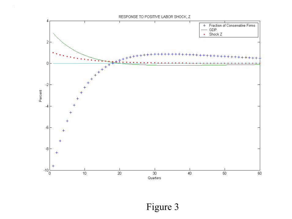
Figure 3

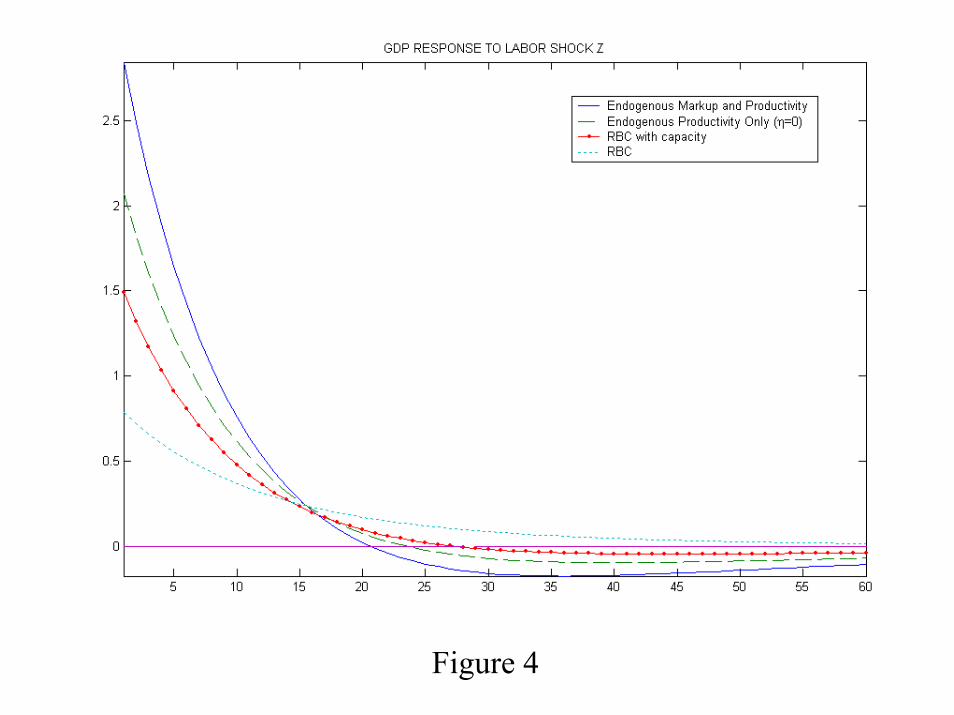
Figure 4

Figure 5

Figure 6

Figure 7

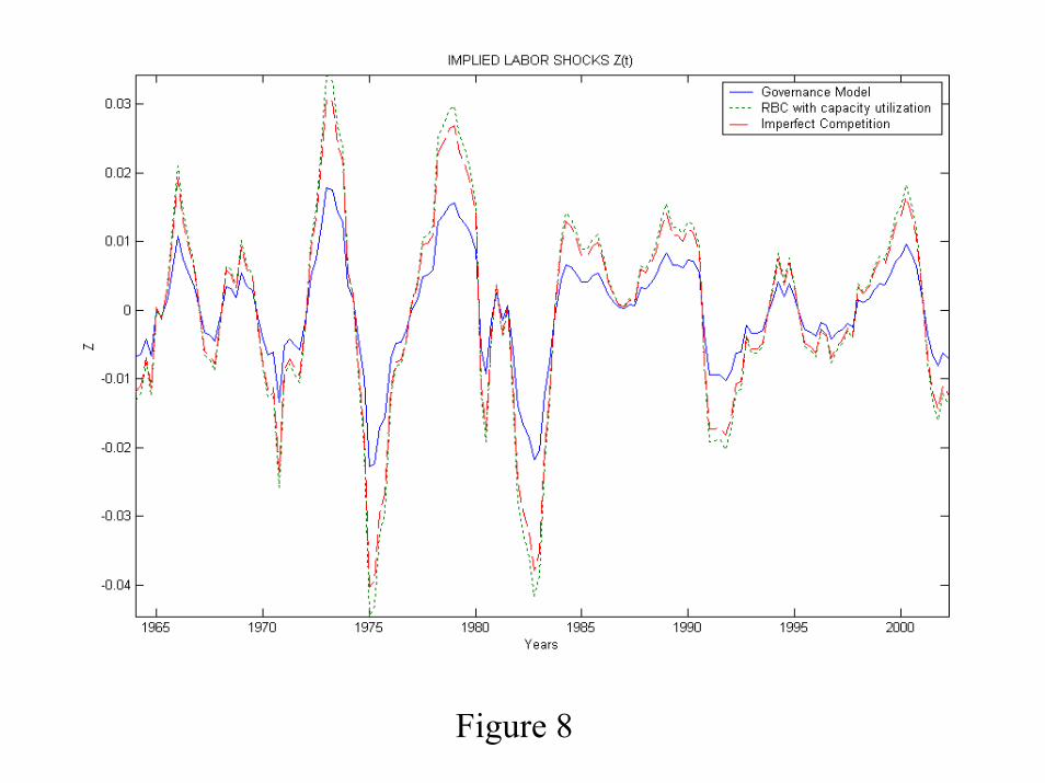
Figure 8

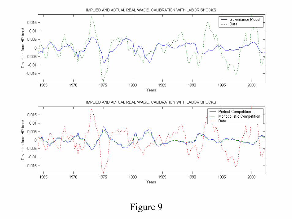
Figure 9

Firm level Volatility of Sales and Employment Growth, All Firmsfiscal year

salesvolat emplovolat

1960 1970 1980 1990 2000

.2

.4

.6

.8

Figure 10Raw standard deviation of log growth rateAnnual Compustat files

Firm level Volatility of Sales Growth, Large Firmsfiscal year

salesvolat_1000 Fitted values

1960 1970 1980 1990 2000

.1

.2

.3

.4

Figure 11Raw standard deviation, firms with more than 1000 employeesAnnual Compustat files

time

rolling gdp volatility firm level volatility trend

1950 1960 1970 1980 1990 2000

0

Figure 12Aggregate rolling window Volatilityand size weighted Firm Level Volatility from Quarterly Compustat filesScaled and demeaned to fit on figure

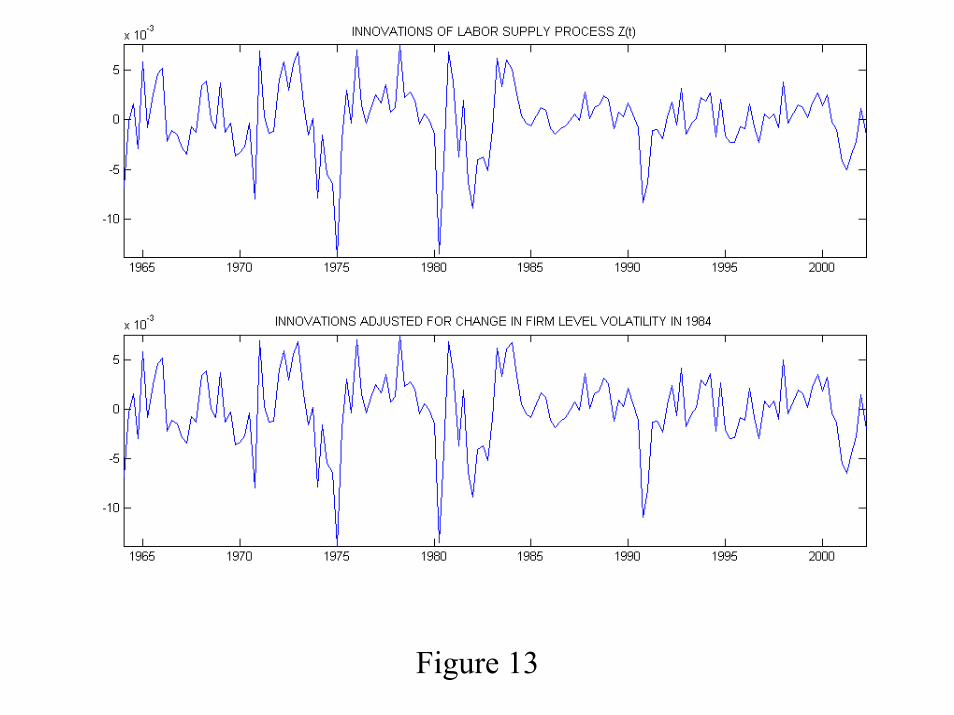
Figure 13