In a U.S. Midcontinent gas field, a channel feature con-tained shale and reservoir sands ranging in porosity from6% to 20%. Well logs, core data, and 3D seismic data werecombined in a reservoir characterization study to map thelithology and variability of porosity within the target sand.The project was conducted in two phases—a qualitative,uncalibrated seismic attribute study and a detailed well-log-calibrated reservoir characterization.

In the first phase, multiple seismic attributes were com-puted and a statistical tool was used to combine them to illu-minate variations in lithology and porosity. These rapidlycomputed “hybrid” attributes can reveal important structuraland stratigraphic features.

In the second phase, well log and core data were usedto calibrate the velocity-porosity relationship. This model wassubsequently used to perturb the porosity of the reservoirsands using representative wells. The resulting “pseudowells” were used as input into a 1D ray-tracing synthetic seis-mic program. Prestack and poststack seismic attributes werecomputed. The well logs were used to classify the geologiccolumn into carbonate, shale, and four different sand poros-ity classes. Aneural network was then trained to relate theseclasses to the modeled seismic attributes. Once trained, thisneural network was used to classify the entire 3D seismicvolume. This classification provided a more reliable indica-tion of higher quality reservoir zones than available from theuncalibrated seismic attributes.

The geologic setting of the study area includesMississippian St. Louis and St. Genevieve carbonates andoverlying Mississippian Chester clastics deposited in a broad,flat shelf environment north of the deep Anadarko Basin.The Chester sands targeted by this study were deposited ina narrow channel cut through the St. Genevieve carbonatesand into the underlying St. Louis limestone. At the end ofMeramacian deposition (St. Genevieve), sea level dropped,exposing the broad carbonate platform. A major fluvial sys-tem and its tributaries flowed across this surface, cutting ashallow valley several miles wide. Upon further sea leveldrop, the river channel incised itself into the St. Genevieve,cutting a wide canyon (750-1000 ft) to depth of 200 ft for manytens of miles. Some of the lowest sands in the channel maybe remnant deposits of this fluvial system, but most sandand shale filling the incisement are Chester-age estuarine sed-iments deposited during multiple transgressive events.Finally, the whole system was buried by the marine Notchshale during maximum flooding.

Data and attribute generation. The 3D seismic survey in thearea of interest covers about 25 square miles. The survey wasof good quality with a broad-frequency bandwidth and a

central frequency of about 50 Hz. Figure 1 shows the inputdata set flattened on the top of the reservoir.

Seismic attributes computed on the 3D volume over thetarget reservoir included envelope, first derivative of enve-lope, second derivative of envelope, instantaneous phase,instantaneous frequency, relative acoustic impedance, litho-logic indicator, similarity, and thin-bed indicator.

Figure 2 shows the relative acoustic impedance attribute20 ms below the top of the reservoir. Figure 3 shows the sim-ilarity attribute, which highlights lateral variation in seismiccharacter. All attributes were combined in a statistical clas-sification system known as Kohonen Self-Organizing Maps(SOMs). Our implementation of SOM is a volume-basedmultiattribute, multidomain clustering system that identi-fies regions of common characteristics based on attributeproperties. In the classified SOM image in Figure 4, theincised channel and other features are clearly visible.

The next step involved incorporation of calibration infor-mation obtained from the borehole. Fortunately, a compre-hensive suite of log curves, excluding shear-wave data, wasavailable for each well in Figure 1.

A core analysis report for about 100 ft of the reservoirinterval from one well was also used. The porosity estimatefrom the density log, and the volume of clay predicted from

428 THE LEADING EDGE MAY 2002 MAY 2002 THE LEADING EDGE 0000

Seismic reservoir characterization of a U.S.Midcontinent fluvial system using rockphysics, poststack seismic attributes, andneural networks

JOEL D. WALLS, M. TURHAN TANER, GARETH TAYLOR, MAGGIE SMITH, MATTHEW CARR, and NAUM DERZHI, RockSolid Images, Houston, Texas, U.S.

JOCK DRUMMOND, DONN MCGUIRE, STAN MORRIS, JOHN BREGAR, and JAMES LAKINGS, Anadarko PetroleumCorporation, Houston, Texas, U.S.

INTE

RP

RE

TE

R’S

CORNERC

oord

inat

ed b

y Li

nda

R. S

tern

bach

Figure 1. Input data set flattened on top of the reservoir.The feature of exploration interest is the channel orscour feature that runs NE-SW. A few other channelsalso may be prospective. The 3D survey over the areacovered about 25 square miles. The survey was of goodquality with a broad-frequency bandwidth and a centralfrequency of about 50 Hz.

SP and gamma-ray logs showed good agreement with val-ues from the core data. Similar log analyses were performedfor the other wells and used to determine lithologies and therange of porosity to be modeled.

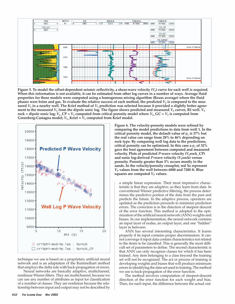
To model the offset-dependent seismic reflectivity, ashear-wave velocity (VS) curve for each well is required.When this information is not available, it can be estimatedfrom other log curves in a number of ways. To evaluate therelative success of each method, predicted VS was comparedto measured VS in a nearby well. The Krief method wasselected because it provided a slightly better agreement tomeasured VS from the dipole sonic log than the others (Figure5).

To create pseudowells in which porosity of the reservoirinterval is perturbed from its actual value, a relationship mustbe found that relates VP, VS, and density to porosity. Onerelationship that worked quite well for modeling the reser-voir sand intervals is Nur’s (1991) critical porosity model.Average fluid properties for the porosity models and VS pre-dictions were computed using a homogenous mixing algo-rithm (Reuss average) in which the fluid phases were brineand gas. Properties of the brine and gas at reservoir condi-tions were computed using the Batzle-Wang (1992) relations.

The velocity-porosity models were refined by compar-

ing model predictions to data from well 1 (Figure 6). In thecritical porosity model, the default value of φc is 37% but thereal value can range from 28% to 46%, depending on rocktype. By comparing well log data to predictions, criticalporosity can be optimized. In this case a φc of 32% gave thebest agreement between computed and measured velocity.In the velocity/porosity plot (Figure 6); red Xs represent VPvalues from the well between 6800 and 7200 ft. Blue squaresare computed VP values, as described above.

Over the reservoir sand interval, we substituted fixedporosity values for the original porosity values and recom-puted new VP, VS, and density curves (Figure 7). This wasdone using a “differential rock physics” approach whichhonors actual log VP and VS values. The procedure consistsof computing VP and VS from the model at the actual wellporosity for each depth in the log. Next, VP and VS are com-puted at the desired or replacement porosity for each depthin the log. The ratio of these modeled velocity values for eachdepth is multiplied by the original measured VP or VS to getthe new replacement velocity. The same approach is appliedto the density log.

Modeling and synthetics. After analysis of well logs, sixlithology classes were defined: shale, carbonate and sandswith 5%, 10%, 15%, and 20% porosity. Gas saturation for eachmodeled case was the original in-situ saturation. A waveletextracted from the data was used to generate synthetic seis-mograms.

Offset and stacked synthetics were generated using 16offsets ranging from 0 to 7040 ft, a range representative ofthe seismic data. Ray tracing was performed over the depthinterval 6750-7200 ft. Figure 8 is a representative display ofthe stacked synthetics and modeled wells.

From the synthetic seismograms at each well, a suite of11 poststack and 2 prestack attributes, computed from thesynthetics, was examined to determine those with the high-est sensitivity to the rock physics modeling. These seven com-puted attributes can be computed on single traces, so theydo not include any geometric attributes. These attributes areenvelope, first derivative of envelope, second derivative ofenvelope, instantaneous phase, instantaneous frequency,thin-bed indicator, and relative acoustic impedance.

Anumber of approaches combine well-log-derived infor-mation and seismic attributes to predict rock properties. The

430 THE LEADING EDGE MAY 2002 MAY 2002 THE LEADING EDGE 0000

Figure 2. The relative acoustic impedance attribute 20 msbelow the top of the reservoir.

Figure 3. Similarity is a geometric attribute that high-lights lateral changes in seismic character. It provides aclear image of the reservoir channel feature.

Figure 4. The classified Kohonen Self-Organizing Maps(SOM). SOM is a volume-based multiattribute, multido-main clustering system that identifies regions of com-mon characteristics based on attribute properties.

technique we use is based on a proprietary artificial neuralnetwork and is an adaptation of the Rummelhart methodthat employs the delta rule with back-propagation of errors.

Neural networks are basically adaptive, multichannel,nonlinear Wiener filters. They are multichannel, because wecan use any number of attributes as input for classificationof a number of classes. They are nonlinear because the rela-tionship between input and output may not be described by

a simple linear expression. Their most impressive charac-teristic is that they are adaptive, so they learn from data. Inconventional Wiener predictive filtering, the process deter-mines the predictive portion of the data from the past andpredicts the future. In the adaptive process, operators areupdated as the prediction proceeds to minimize predictionerrors. The correction is in the direction of steepest descentof the error function. This method is adopted to the opti-mization of the artificial neural network (ANN) weights andbiases. In our implementation, the neural network containsan input layer of nodes, an output layer, and one “hidden”layer in between.

ANN has several interesting characteristics. It learnsproperly if its input contains proper discriminators. It can-not converge if input data contain characteristics not relatedto the items to be classified. This is generally the most diffi-cult set of parameters to define. The second characteristic isthat ANN can only recognize classes for which it has beentrained. Any item belonging to a class beyond the trainingset will not be recognized. The act or process of training isdeveloping weights and biases that will produce minimumerrors in identifying the data set used in training. The methodwe use is back-propagation of the error function.

The method involves computation of steepest-descentdirection of the error function for each weight and bias.Then, for each input, the difference between the actual out-

432 THE LEADING EDGE MAY 2002 MAY 2002 THE LEADING EDGE 0000

Figure 6. The velocity-porosity models were refined bycomparing the model predictions to data from well 1. In thecritical porosity model, the default value of φc is 37% butthe real value can range from 28% to 46% depending onrock type. By comparing well log data to the predictions,critical porosity can be optimized. In this case a φc of 32%gave the best agreement between computed and measuredvelocity. Plots of predicted P-wave velocity (VProck_CP)and sonic log-derived P-wave velocity (VProck) versusporosity. Porosity greater than 5% occurs mostly in thesands. In the velocity/porosity crossplot, red Xs representVP values from the well between 6800 and 7200 ft. Bluesquares are computed VP values.

Figure 5. To model the offset-dependent seismic reflectivity, a shear-wave velocity (VS) curve for each well is required.When this information is not available, it can be estimated from other log curves in a number of ways. Average fluidproperties for these models were computed using a homogenous mixing algorithm (Reuss average) where the fluidphases were brine and gas. To evaluate the relative success of each method, the predicted VS is compared to the mea-sured VS in a nearby well. The Krief method of VS prediction was selected because it provided a slightly better agree-ment to the measured VS from the dipole sonic log. The figure shows predicted and measured VS curves, B2 well. VSrock = dipole sonic log; VS_CP = VS computed from critical porosity model where VS_GC = VS is computed fromGreenberg-Castagna model; VS_Krief = VS computed from Krief model.

put and the desired output is computed. This is the error,which is distributed as in adaptive filtering along the net-work starting from the output layer back toward the inputlayer according to the error gradient at each node. Themethod will adjust each weight by a small amount with eachtraining data set. The rms velocity and absolute error aremonitored during the iteration. Once the amount of error isreduced to a satisfactory level, the ANN is deemed trained.In most instances, known data are kept out of the trainingdata set and used to verify the training.

The iterative training process was performed until theneural network developed a set of weights and scalars thatminimized discrepancies between predicted results and theactual classes at the training wells. At that point, the networkwas considered to have achieved acceptable convergence andto be well trained.

The classification for lithology and porosity produced

extremely encouraging results. The neural network wastrained on two calibration wells, each modeled for porosityvariation in the sand. Figure 9, an example of the results ofthe training on well 1, shows four pairs of lithology columns.In each pair, the column on the right shows the well-log-derived lithology classes (with porosity replacement zoneindicated by red vertical bar). The column on the left showsthe ANN-predicted lithology classes. For each porosity case,the calibrated neural network was able to locate the sandand predict its porosity. The success rate for predicting thecorrect porosity class in the sands was greater than 80% forthe calibration wells.

Interwell classification. The trained neural network devel-oped from the calibration wells was then applied to the realseismic data. Separate lithology and porosity classificationswere performed on a sample-by-sample basis on attributescomputed from the entire 3D seismic volume using the

434 THE LEADING EDGE MAY 2002 MAY 2002 THE LEADING EDGE 0000

Figure 9. Results of neural network classification at well1. In each pair, the column on the right shows the well-log-derived lithology classes (with porosity replacementzone indicated by red vertical bar). The column on theleft shows ANN-predicted lithology classes. For eachcase, the calibrated neural network was able to locatethe sand and predict its porosity. The success rate forpredicting the correct porosity class in the sands wasgreater than 80% for the calibration wells.

Figure 7. Over the reservoir sand interval, we substituted fixed porosity values for the original porosity values andrecomputed new VP, VS, and density curves. This was done using a “differential rock physics” approach which honorsactual log-measured VP and VS.

Figure 8. A representative display of the stacked syn-thetics and modeled wells, pseudowell density, andsonic logs with corresponding stacked synthetic traces.Based on analysis of well data, six lithology classes weredefined: shale, carbonate and sands with 5%, 10%, 15%and 20% porosity. Gas saturation for each of the mod-eled cases was the original in-situ saturation. A waveletextracted from the data was used to generate the syn-thetic seismograms.

derived neural weights and scalars. Figure 10 is a flattenedtime slice through the volume classified for lithology andporosity.

We have compared the lithology from the calibrated seis-mic attribute-based reservoir characterization to the well-logdata in six wells. Figure 11 shows a cross section of the lithol-ogy volume through well 1. The gamma-ray and SP-logcurves are superimposed over the lithology classes betweenpoints A and A”. There is good agreement between the log-indicated sand section and the sand classification computedfrom the trained neural network applied to the 3D seismicattribute volume.

However, due to stratigraphic variations within the chan-nel, the neural net classification does not always properlycharacterize all reservoir variations within the analysis win-dow. It is limited to characterizing only those wells that fit

within the range of reservoir variations of the selected wells.Classifications of other combinations of wells in the studyshowed that different weights and scalars for the same setof attributes are necessary to produce similar agreementbetween observed and predicted sand sections. The finaltraining network was chosen to identify the characteristicsof the wells with the most similar reservoir stratigraphy.

Since the project was completed, we have learned thatsome sands in some withheld wells in the channel are wet,not gas-filled as we had originally believed. Future work inthis area should include more wet sand classification in addi-tion to the gas-filled, multiple porosity classes, to sample moreof the reservoir complexity.

Warning! A common assumption is that higher-porositysands cause higher reflection amplitudes. However, our cal-ibrated classification shows that this is not true in some areasof our data set. Figure 12 shows that some high-porosityzones are in regions that have lower amplitude (black cir-cle), and others do correspond to high-amplitude areas.

Conclusions. Seismic attributes were computed on a 3Dseismic volume over a sand-filled channel in the UnitedStates Midcontinent. These attributes were classified usingboth supervised and unsupervised methods. The unsuper-vised classifications were helpful in defining the extent andshape of the reservoir sands. A trained artificial neural net-work using poststack seismic attributes was able to classifythe seismic data volume for lithology, porosity, and thick-ness in the targeted sands with an acceptable degree of con-fidence.

Suggested reading. “Seismic properties of pore fluids” by Batzleand Wang (GEOPHYSICS, 1992). “A petrophysical interpretationusing the velocities of P and S waves (full-waveform sonic)” byKrief et al. (The Log Analyst, 1990). “Neural computing in geo-physics” by McCormack (TLE, 1991). “Complex seismic traceanalysis” by Taner et al. (GEOPHYSICS, 1979). “Seismic attributesrevisited” by Taner et al. (SEG 1994 Expanded Abstracts). “Wavevelocities in sediments” by Nur et al. (in Wave Velocities inSediments by Hovem et al. (eds), 1991). LE

Acknowledgments: The authors thank Anadarko Petroleum Corp. for per-mission to publish these results.

Corresponding author: j.walls@rocksolidimages.com

436 THE LEADING EDGE MAY 2002 MAY 2002 THE LEADING EDGE 0000

Figure 12. An example in which high amplitude in theinput section (left) does not correspond to high porosityin the classified volume (right). Some high-porosityzones are found in regions that have lower amplitude(black circle), and others correspond to high amplitudeareas.

Figure 10. The trained neural network developed fromthe calibration wells was applied to the real seismicdata. Separate lithology and porosity classifications wereperformed on a sample-by-sample basis on attributescomputed from the entire 3D seismic volume using thederived neural weights and scalars. The image shows aflattened time slice through the 3D seismic volume clas-sified for lithology and porosity. Colors indicate lithol-ogy and four different sand porosity classes as shown atthe bottom of Figure 11.

Figure 11. Cross section of lithology volume passingthrough well 1. Gamma-ray and SP log curves are super-imposed over the lithology classes between points Aand A”. There is good agreement between the log-indi-cated sand section and the sand classification computedfrom the trained neural network and applied to the 3Dseismic-attribute volume.